Decentralized Estimation using Distortion …tua95067/grbovic_prl_2013.pdfDecentralized Estimation...
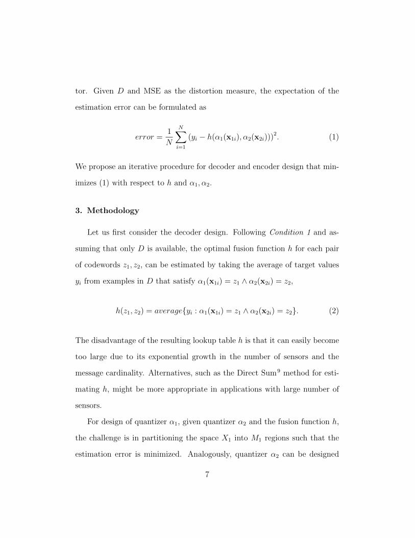
29
Decentralized Estimation using Distortion Sensitive Learning Vector Quantization Mihajlo Grbovic and Slobodan Vucetic Department of Computer and Information Sciences, Temple University, Philadelphia, PA 19122, USA Abstract A typical approach in supervised learning when data comes from multiple sources is to send original data from all sources to a central location and train a predictor that estimates a certain target quantity. This can be inef- ficient and costly in applications with constrained communication channels, due to limited power and/or bitlength constraints. Under such constraints, one potential solution is to send encoded data from sources and use a de- coder at the central location. Data at each source is summarized into a single codeword and sent to a central location, where a target quantity is estimated using received codewords. This problem is known as Decentralized Estima- tion. In this paper we propose a variant of the Learning Vector Quantization (LVQ) classification algorithm, the Distortion Sensitive LVQ (DSLVQ), to be used for encoder design in decentralized estimation. Unlike most related research that assumes known distributions of source observations, we assume * Corresponding author, tel: (215) 204 - 7230, fax: (215) 204-5082 Email address: [email protected], [email protected] (Mihajlo Grbovic and Slobodan Vucetic) Preprint submitted to Pattern Recognition Letters August 16, 2014
-
Upload
dangnguyet -
Category
Documents
-
view
223 -
download
0
Transcript of Decentralized Estimation using Distortion …tua95067/grbovic_prl_2013.pdfDecentralized Estimation...
Decentralized Estimation using Distortion Sensitive
Learning Vector Quantization
Mihajlo Grbovic and Slobodan Vucetic
Department of Computer and Information Sciences, Temple University, Philadelphia, PA19122, USA
Abstract
A typical approach in supervised learning when data comes from multiple
sources is to send original data from all sources to a central location and
train a predictor that estimates a certain target quantity. This can be inef-
ficient and costly in applications with constrained communication channels,
due to limited power and/or bitlength constraints. Under such constraints,
one potential solution is to send encoded data from sources and use a de-
coder at the central location. Data at each source is summarized into a single
codeword and sent to a central location, where a target quantity is estimated
using received codewords. This problem is known as Decentralized Estima-
tion. In this paper we propose a variant of the Learning Vector Quantization
(LVQ) classification algorithm, the Distortion Sensitive LVQ (DSLVQ), to
be used for encoder design in decentralized estimation. Unlike most related
research that assumes known distributions of source observations, we assume
∗Corresponding author, tel: (215) 204 - 7230, fax: (215) 204-5082Email address: [email protected], [email protected]
(Mihajlo Grbovic and Slobodan Vucetic)
Preprint submitted to Pattern Recognition Letters August 16, 2014
that only a set of empirical samples is available. DSLVQ approach is com-
pared to previously proposed Regression Tree and Deterministic Annealing
(DA) approaches for encoder design in the same setting. While Regression
Tree is very fast to train, it is limited to encoder regions with axis-parallel
splits. On the other hand, DA is known to provide state-of-the-art perfor-
mance. However, its training complexity grows with the number of sources
that have different data distributions, due to over-parametrization. Our ex-
periments on several synthetic and one real-world remote sensing problem
show that DA has limited application potential as it is highly impractical
to train even in a four-source setting, while DSLVQ is as simple and fast to
train as the Regression Tree. In addition, DSLVQ shows similar performance
to DA in experiments with small number of sources and outperforms DA in
experiments with large number of sources, while consistently outperforming
the Regression Tree algorithm.
Keywords: Quantization, Distributed estimation, Non-linear estimation,
vector quantization, Aerosol retrieval
1. Introduction
In the decentralized estimation setup, the physical quantities (e.g., tem-
perature, pressure) are measured at distributed locations by sensor devices
with limited energy and memory capacities and sent via constrained com-
munication channels to a fusion center where a desired target variable is
estimated. With advances in sensing technology, there is a growing interest
2

in designing decentralized estimation systems with sensors that provide mul-
tivariate observations (e.g., camera sensor networks) and multi-type sensors
that measure different quantities (e.g. power plants). The target variable y
can be either a continuous quantity to be estimated from noisy sensor obser-
vations of the same type x = y + noise, a continuous function of potentially
multi-type and multi-dimensional sensor observations x or a binary variable
that indicates a certain event. In the literature, Decentralized Detection1,2
is used for categorical target and Decentralized Estimation for numerical
target. Applications of Decentralized Estimation can be found in remote-
sensing, sonar and seismology systems. It has been a focus of considerable
research in the past two decades3,4,5,6,7,8,9,10.
Given a bitlength constraint on messages, the sensors can transmit only
a summary message instead of the original measurement. The principal ap-
proach is to design encoders at sensor sites and a decoder at the fusion site
that reconstructs the target variable from the received encoder messages.
The encoder types range from linear threshold-based quantizers4,2,5 to non-
linear decision tree-7, nearest prototype-6,8 and kernel-based1 quantizers. In
most previous work, encoder design is carried out by assuming that the joint
distribution P(x, y) is known3,2,5,4,11. In practice this is violated, either be-
cause the parameters of P(x, y) are unknown or even less is known about it.
Here, we consider a more realistic scenario and address the problem using
a set of empirical samples of sensor and target measurements7,8,6. In many
real-world applications it is reasonable to assume that certain amount of
3

source an target data can be collected for purposes of encoder and decoder
design. Finally, unlike some methods4,10 that require sensors to communi-
cate among themselves, we consider systems where each sensor communicates
only with the fusion center. This setup is favorable as it does not increase the
communication cost on account of solving the bitlength constraint problem.
The proposed methodology was evaluated on several synthetic problems
with different number of sources and on a real-world problem of predicting
aerosol optical depth (AOD) from remotely sensed data. Multisource ob-
servations in form of multispectral images are collected from sensors aboard
satellites across the entire globe, while target AOD observations are collected
from limited number of ground-based sensors placed at world-wide locations.
The collocated data are used to train encoders for satellites and a decoder
for AOD prediction, which reduces communication cost and allows prediction
across the entire globe.
2. Problem Setup
The general setup assumes a system of n distributed data sources S1, ..., Sn
that produce multivariate vectors x1, ...,xn drawn from probability distribu-
tion P(x1, ...,xn), and a fusion center (Figure 1). It is assumed that the
random vectors xi, i = 1, ..., n, are related to the unobservable continuous
quantity y that the fusion center needs to estimate and there exists a joint
distribution P(x1, ...,xn, y).
Due to the channel bandwidth and energy constraints, the i-th sensor
4

S1
S2
datasources
Sn
h
xn
x2
x1
z1
z2
zn
_1
_2
_n
y_
encoders
original data codewords
decoder
Figure 1: Illustration of the Decentralized Estimation System
communication is limited to Mi codewords. Let αi be the quantization func-
tion for source Si. Instead of the original vectors, x1, ...,xn, the data sources
transmit quantized messages z1, ..., zn, zi = αi(xi), to the fusion center, where
zi is as an integer from set {1, ...,Mi}. Let h be the function of the fusion
center that gives the estimate y = h(z1, ..., zn) of y, given the quantizers
α1, ..., αn. At the fusion center, the goal is to find the point estimate of y
that minimizes the distortion measure d. The optimal estimate in this case
is the conditional expectation of a random vector Y , E(Y |x1, ...,xn).
Under this setup, the problem of decentralized estimation is to find the
quantization functions α1, ..., αn and the fusion function h such that the es-
timation error EX [d{EY (Y |X1, ..., Xn), h(α1(X1), ..., αn(Xn))}] is minimized
under given communication constraints. Special case of the estimation error
under assumption that d is defined as the Mean Squared Error was formu-
5
lated in9 as error = EX [(EY (Y |X1, ..., Xn)− h(α1(X1), ..., αn(Xn)))2].
For decentralized estimation with the squared error distortion, when the
joint probability distribution P(x1, ...,xn, y) is known, necessary conditions
for the optimal compression functions α1, ..., αn and fusion function h were
derived3. Assuming, without loss of generality, that n = 2, they are:
Condition 1 (Decoder design). Given α1 and α2, the optimal h is given
by h(z1, z2) = E(Y |α1(x1) = z1, α2(x2) = z2), where z1 ∈ {1, ...,M1} and
z2 ∈ {1, ...,M2}.
Condition 2 (Encoder design). Given α2 and h, optimal quantization function
α1 is determined as α1(x1) = arg minj EX2 [(EY (Y |x1, X2)− h(j, α2(X2)))2],
where j ∈ {1, ...,M1}.
The conditions lead to the solution by the generalized Lloyd’s algorithm
where the construction of the decentralized system is performed iteratively.
One step consists of optimizing the fusion function h while fixing the local
quantization functions at each sensor, whereas another step involves opti-
mizing the quantization function at a given sensor while fixing h and the
quantization functions of the remaining sensors.
The problem addressed in this paper arises when only a set of examples
from the underlying distribution P(x1,x2, y) is available, D = {(x1i,x2i, yi), i =
1, ..., N}, where x1i is a K1-dimensional vector and x2i a K2-dimensional vec-
6
tor. Given D and MSE as the distortion measure, the expectation of the
estimation error can be formulated as
error =1
N
N∑i=1
(yi − h(α1(x1i), α2(x2i)))2. (1)
We propose an iterative procedure for decoder and encoder design that min-
imizes (1) with respect to h and α1, α2.
3. Methodology
Let us first consider the decoder design. Following Condition 1 and as-
suming that only D is available, the optimal fusion function h for each pair
of codewords z1, z2, can be estimated by taking the average of target values
yi from examples in D that satisfy α1(x1i) = z1 ∧ α2(x2i) = z2,
h(z1, z2) = average{yi : α1(x1i) = z1 ∧ α2(x2i) = z2}. (2)
The disadvantage of the resulting lookup table h is that it can easily become
too large due to its exponential growth in the number of sensors and the
message cardinality. Alternatives, such as the Direct Sum9 method for esti-
mating h, might be more appropriate in applications with large number of
sensors.
For design of quantizer α1, given quantizer α2 and the fusion function h,
the challenge is in partitioning the space X1 into M1 regions such that the
estimation error is minimized. Analogously, quantizer α2 can be designed
7
given α1 and h. One viable approach is based on the recursive partitioning
of the X1 space using the Regression Trees7. An alternative, studied in this
paper, is the multi-prototype approach.
In the multi-prototype approach, quantizer α1 consists of M1 regions,
where each region Rj, j = 1, ...,M1 is represented as a union of Voronoi cells
defined by a set of prototypes. Thus, α1 is completely defined by a set of P
prototypes {(mk, ck), k = 1, ..., P}, where mk is a K-dimensional vector in
input space and ck is its assignment label, defining to which of the M1 re-
gions/codewords it belongs. The input x1i is compared to all prototypes and
its codeword z1i is assigned as the assignment label of its nearest prototype,
z1i = cl, l = arg mink(de(x1i,mk)), where de is the Euclidean distance.
Following this setup, given D, we can restate Condition 2 as finding the
optimal set of prototypes to minimize the overall distortion of quantizer α1
L =N∑i=1
d(yi, h(z1i, α2(x2i)), (3)
where distortion d is the squared error,
d(yi, h(z1i, α2(x2i)) = (yi, h(z1i − α2(x2i))2. (4)
Finding {(mk, ck), k = 1, ..., P} that minimize (3) is challenging. We consider
several approaches.
Hard Classification Approach. One approach to minimize (3) is to
convert the problem of encoder design to classification. To design α1 in
8
this manner, in each iteration we use the original training data set D to
create a new data set, D1 = (x1i, q1i), i = 1, ..., N , where q1i is the codeword
with the smallest error, q1i = arg minj (yi − h(j, α2(x2i)))2. The goal then
becomes finding a set of prototypes, {(mk, ck), k = 1, ..., P}, that minimize
the classification error on D1. Nearest Prototype Classification algorithms,
such as Learning Vector Quantization (LVQ)12, can be used for this purpose6.
Let us consider the LVQ2 algorithm12 which starts from an initial set
of prototypes, and reads the training data points sequentially to update the
prototypes. LVQ2 considers only the two closest prototypes. Three condi-
tions have to be met to update the two closest prototypes: 1) Class of the
prototype closest to x1i has to be different from z1i, 2) Class of the second
closest prototype has to be equal to z1i, and 3) x1i must satisfy the ”win-
dow rule” by falling near the hyperplane at the midpoint between the closest
(mA) and the second closest prototype (mB). These two prototypes are then
modified as
mt+1A = mt
A − η(t)(x1i −mtA)
mt+1B = mt
B + η(t)(x1i −mtB), (5)
where t counts how many updates have been made, and η(t) is a monotoni-
cally decreasing function of t.
Let dA and dB be the distances between x1i and mA and mB. Then, the
”window rule”, that was introduced to prevent divergence12, is satisfied if
9
min(dB/dA, dA/dB) > w, where w is a constant commonly chosen between
0.4 and 0.8
Soft Classification Approach. The potential issue with the hard clas-
sification approach is that it enforces assignment of a data point to the code-
word with the minimum squared error (4). This can be too aggressive, con-
sidering that there might be other codewords resulting in a similar squared
error. The soft classification approach addresses this issue. Instead of as-
signing a data point to the closest prototype, let us consider a probabilistic
assignment pij = P(z1i = j|x1i) defined as the probability of assigning i-th
data point to j-th codeword. The objective (3) can now be reformulated as
L =N∑i=1
M1∑j=1
pijd(yi, h(z1i, α2(x2i))) =N∑i=1
M1∑j=1
pije(i, j), (6)
where e(i, j) = d(yi, h(z1i, α2(x2i))) was introduced to simplify the notation.
Objective (6) is an approximation of (3) that allows us to find a computation-
ally efficient solution. We use a mixture model to calculate the assignment
probabilities pij. Let us assume that the probability density P(x1) of the
observation at the first sensor can be described by mixture
P(x1) =P∑k=1
P(x1|mk)P(mk), (7)
where P(x1|mk) is a conditional probability that prototype mk generates ob-
servation x1 and P(mk) is the prior probability. We represent the conditional
10

density function P(x1|mk) as the Gaussian distribution with mean mk and
standard deviation σs. Let us denote gik ≡ P(mk|x1i) as the probability
that i-th data point was generated by k-th prototype. By assuming that all
prototypes have the same prior, P(mk) = 1/P , and using the Bayes’ rule,
gik can be updated as
gik =exp(−(x1i −mk)/2σ
2s)
P∑l=1
exp(−(x1i −ml)/2σ2s)
. (8)
The probability pij can be obtained using (8) as
pij =
∑j:ck=j
exp(−(x1i −mk)/2σ2s)
P∑l=1
exp(−(x1i −ml)/2σ2s)
. (9)
In soft classification approach, the objective of learning is to estimate the
prototype positions mk, k = 1, ..., P , by minimizing (6). This can be done
using the stochastic gradient descent, where at t-th update the prototypes
are calculated as
mt+1k = mt
k − η(t) · (e(i, ck)−M1∑j=1
pije(i, j)) · gik(x1i −mt
k)
σ2s
(10)
We will refer to this as the Soft Prototype Quantization (SPQ)
Parameter σs controls the fuzziness of the distribution. For σs = 0 the
assignments become deterministic, and (6) is equivalent to (3). If σs → ∞
11

the assignments become uniform, regardless of the distance. One option is
that σ2s be treated as a parameter to be optimized such that (6) is minimized.
It is not necessarily the best approach since minimizing (6) does not imply
minimizing (3). In this work, we are treating σ2s as an annealing parameter
that is initially set to a large value and then is decreased towards zero using
σ2s(t+1) = σ2
s(0) ·σT/(σT +t), where σT is the decay parameter. The purpose
of annealing is to facilitate convergence toward a good local optimum of (3).
We note that this strategy has been used in soft prototype approaches by
other researchers13.
Deterministic Annealing (DA) is a generalization of the soft classi-
fication approach. Instead of minimizing (6), it minimizes the regularized
objective,
L = β ·N∑i=1
M1∑j=1
pije(i, j)−H, (11)
where β controls the tradeoff between the objective (6) (first term) and the
entropy H = −∑N
i=1
∑M1
j=1 pij log pij.
In8 authors suggest minimizing L starting at the global minimum for
β = 0 and updating the solution as β increases. As β → ∞ (11) becomes
equivalent to (6). The role of the entropy term is to further improve the
convergence toward a good local optimum. The DA prototype update rule
can be obtained by the stochastic gradient descent as
mt+1k = mt
k − η(t) · (Gi(ck)−M1∑j=1
pijGi(j)) · gik(x1i −mt
k)
σ2s
(12)
12
where Gi(j) = β · e(i, j) + log pij. Parameter σ2s is updated as σ2
s(t + 1) =
σ2s(0) · σT/(σT + t), where σ2
s is reset back to σ2s(0) after each increase of β.
The drawback is that, since the cost function is defined and minimized at
each value of β, the model takes quite long to produce and the convergence
can be quite sensitive to the annealing schedule of β.
Distortion Sensitive Learning Vector Quantization. To apply the
stochastic gradient descent in (10), one should specify the learning rate η(t)
and the annealing rate for σ2s , while for the DA version in (12) the annealing
schedule for β is required too. In this subsection, we show how the update
rule (10) can be simplified such that it does not require use of the parameter
σ2s . The resulting algorithm resembles LVQ2.
Objective (6) is a good approximation of (3) for small values of σ2s . In
this case, assignment probabilities pij of all but the closest prototypes are
near zero. As a result, we approximate (10) by using only the two closest
prototypes. Given x1i, we denote the closest prototype as (mA, cA) and the
second closest as (mB, cB).
Let us consider three major scenarios. First, if mA and mB are in similar
proximity to x1i, their assignment probabilities will be approximately the
same, giA = gjB = 0.5. The prototype update rule from (10) could then be
expressed as
mt+1A = mt
A − η(t)(e(i, cA)− e(i, cB))(x1i −mtA)
mt+1B = mt
B + η(t)(e(i, cA)− e(i, cB))(x1i −mtB), (13)
13
where σ2s is incorporated in the learning rate parameter η. The difference
(e(i, cA)− e(i, cB)) determines the amount of prototype displacement; when
the difference is small the prototype updates are less extreme. The sign of
the difference determines the direction of updates; if e(i, cA) is larger than
e(i, cB), prototype mA is moved away from data point x1i and mB prototype
is moved towards it.
The second scenario is when the closest prototype is much closer than the
second closest, which makes giB ∼ 0. Following (10), none of the prototypes
are updated. Taken together, the first two scenarios are equivalent to the
LVQ2 window rule
In the third scenario, the two closest prototypes belong to the same code-
word and, as a consequence of e(i, cA) = e(i, cB), the prototype positions are
not updated.
The three scenarios establish the new algorithm (DSLVQ2): Given x1i,
if the two closest prototypes, mA and mB, have different class labels and
min(dB/dA, dA/dB) > w, update their positions (13), otherwise preserve their
current positions
To avoid settling of prototypes in a bad local minima, SPQ algorithm
uses annealing, while DA uses double annealing. The proposed DSLVQ2
uses a simple and much faster procedure. Harmful prototypes, stuck in local
minima, are identified after every ns(= 10) quantizer design iterations as the
ones whose current label ck is different from label c∗k which introduces the
14
least prediction error amount to its Voronoi cell
c∗k = arg minj{∑
i:x1i∈vk
e(i, j)}, (14)
where vk is Voronoi cell of the k-th prototype. In this case, DSLVQ2 switches
the label from ck to c∗k.
Relationship with LVQ2. When target variable y is categorical instead
of real-valued, we could use 0-1 error, defined as e(i, ck) = δ(yi, h(ck, α2(x2i))),
where δ(·) is the Dirac delta function, instead of the squared error. Now, (13)
reduces to (5). If, in addition, we update prototypes only if e(i, cA) = 1 and
e(i, cB) = 0, DSLVQ2 reduces to LVQ2.
Prototype Initialization and Refinement. Regardless of whether
(5), (10), (12), or (13) are used for prototype update, the algorithm starts
by randomly selecting P points from D and assigning equal number of pro-
totypes to each codeword. Unlike DSLVQ which uses a label replacement
mechanism (14), and DA and SPQ which use annealing, the regular LVQ
algorithm is highly sensitive to initial choice of prototypes. If the initial-
ization is not done in a proper way good results might never be achieved.
Repeating random initialization or using K-means algorithm14 to initialize
the prototypes in case of regular LVQ helps in certain cases.
15
4. Experiments
In order to compare quantizer design using DSLVQ2 algorithm with those
using LVQ2, DA, SPQ, and Regression Tree algorithms, we performed three
sets of experiments with synthetic data and one experiment with real-world
AOD data. The series of experiments were of increasing complexity, meaning
that the number of sources and source features grew. When compared to
the DSLVQ2 algorithm, the DA and SPQ algorithms showed a performance
decrease in out of sample prediction with increase in the number of sources
and source types.
Setup. The algorithms were compared on different budget sizes P , rep-
resenting the number of prototypes and Regression Tree nodes. In syn-
thetic data experiments we used two training data sizes of N = 10, 000
and N = 1, 000 points and a test set of size 10, 000. The experiments were
repeated 10 times and the average test set MSE are reported. Training of
encoders and decoder was terminated when the training set MSE (1) stopped
decreasing by more than 10−5. Experiments were performed on Intel Core
Duo 2.6 GHz processor machines with 2GB of RAM. We also report the to-
tal time needed to design a decentralized system from training data using
different encoder design algorithms.
Parameter Selection. We have empirically observed that the sensitivity
of prototype-based algorithms to parameters varies significantly - they are
fairly robust to some and highly sensitive to others. The learning rate η is
universal for all algorithms. We initially set it to η0 = 0.03 and update it
16

Table 1: Parameter Search GridParameter Start Value Search Step End Value
σ2s 0.3 +0.3 sensor s data variance + 0.3
σT 5N ×2 40N
β0 0.01 ×2 0.08
βT 1.05 +0.05 1.2
using η(t) = η0 ·ηT/(ηT + t), where ηT = 8N . The window parameter w, used
in LVQ2 and DSLVQ2, is easy to adjust and was fixed to a value of w = 0.7.
A common practice8 for annealing the DA parameter β is to initially set
it to a small value (e.g. 0.01) and update it using βt+1 = βT · βt, where
βT = 1.11. Parameter σ2s for sensor S is often13 initialized as the sensor data
variance and updated using the annealing schedule with σT = 8N . However,
our preliminary experiments revealed that DA and SPQ are very sensitive to
these parameters. As a result, parameters σ2s , σT , βT , β0 have to be adjusted
from case to case depending on K, P and N .
Parameter search for DA and SPQ algorithms was based on the grid
displayed in Table 1. The best parameters were chosen as the ones that
achieve the lowest MSE on the validation set, formed by randomly selecting
25% of the training data. The same validation set was used for Regression
Tree pruning.
We note that if the sensors differ in type because they measure different
quantities, the choice of σ2s becomes more involved as appropriate σ2
s would
differ for each type of sensor. If the best σ2s for a single sensor type s is found
in os training steps, the best combination of σ2s values for T sensor types is
found in o1 · o2 · ... · oT training steps.
17
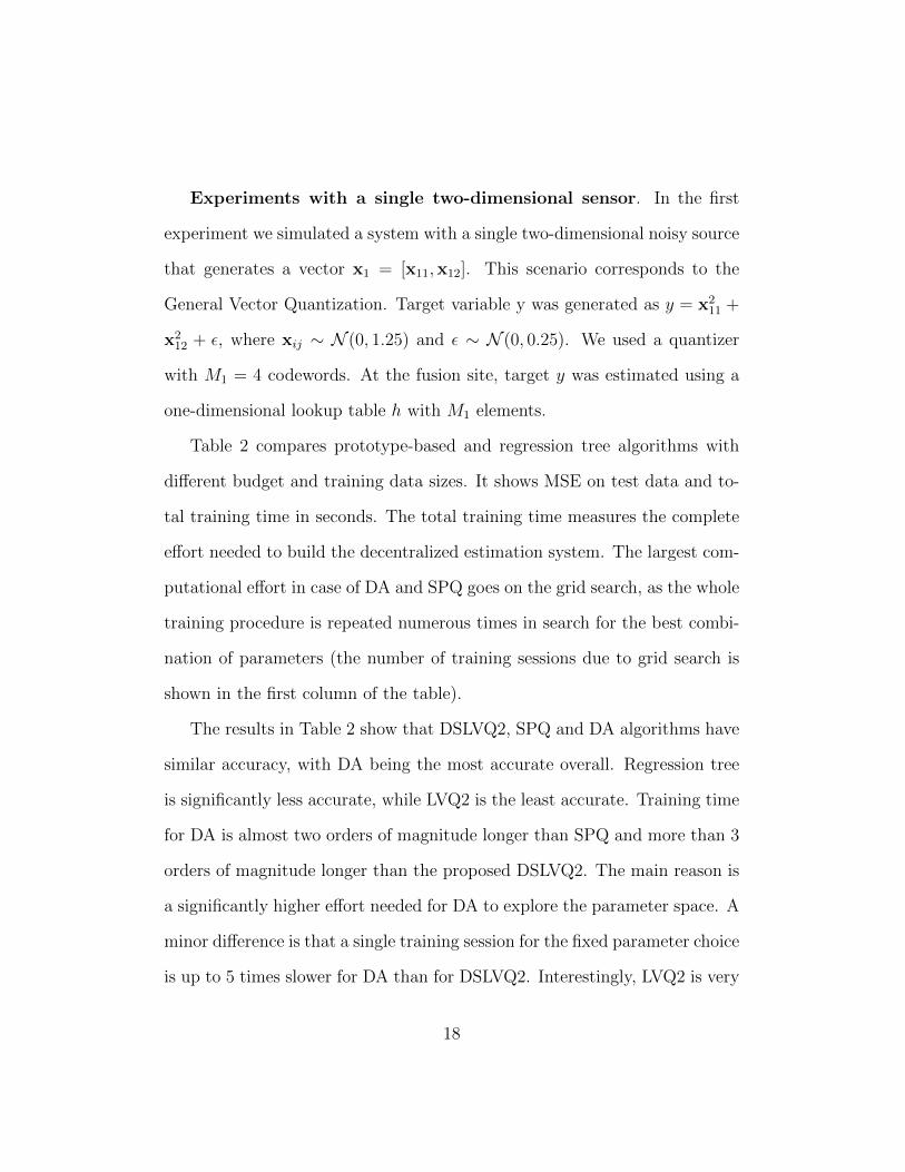
Experiments with a single two-dimensional sensor. In the first
experiment we simulated a system with a single two-dimensional noisy source
that generates a vector x1 = [x11,x12]. This scenario corresponds to the
General Vector Quantization. Target variable y was generated as y = x211 +
x212 + ε, where xij ∼ N (0, 1.25) and ε ∼ N (0, 0.25). We used a quantizer
with M1 = 4 codewords. At the fusion site, target y was estimated using a
one-dimensional lookup table h with M1 elements.
Table 2 compares prototype-based and regression tree algorithms with
different budget and training data sizes. It shows MSE on test data and to-
tal training time in seconds. The total training time measures the complete
effort needed to build the decentralized estimation system. The largest com-
putational effort in case of DA and SPQ goes on the grid search, as the whole
training procedure is repeated numerous times in search for the best combi-
nation of parameters (the number of training sessions due to grid search is
shown in the first column of the table).
The results in Table 2 show that DSLVQ2, SPQ and DA algorithms have
similar accuracy, with DA being the most accurate overall. Regression tree
is significantly less accurate, while LVQ2 is the least accurate. Training time
for DA is almost two orders of magnitude longer than SPQ and more than 3
orders of magnitude longer than the proposed DSLVQ2. The main reason is
a significantly higher effort needed for DA to explore the parameter space. A
minor difference is that a single training session for the fixed parameter choice
is up to 5 times slower for DA than for DSLVQ2. Interestingly, LVQ2 is very
18
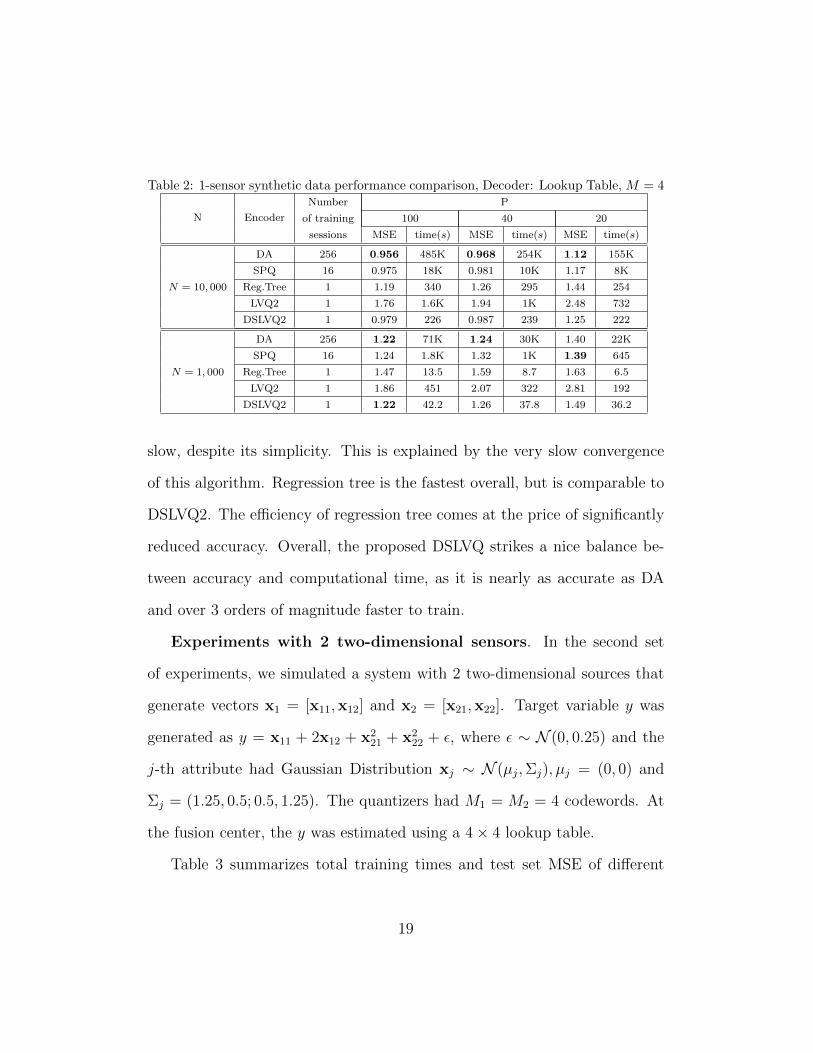
Table 2: 1-sensor synthetic data performance comparison, Decoder: Lookup Table, M = 4
N Encoder
Number P
of training 100 40 20
sessions MSE time(s) MSE time(s) MSE time(s)
DA 256 0.956 485K 0.968 254K 1.12 155K
SPQ 16 0.975 18K 0.981 10K 1.17 8K
N = 10, 000 Reg.Tree 1 1.19 340 1.26 295 1.44 254
LVQ2 1 1.76 1.6K 1.94 1K 2.48 732
DSLVQ2 1 0.979 226 0.987 239 1.25 222
DA 256 1.22 71K 1.24 30K 1.40 22K
SPQ 16 1.24 1.8K 1.32 1K 1.39 645
N = 1, 000 Reg.Tree 1 1.47 13.5 1.59 8.7 1.63 6.5
LVQ2 1 1.86 451 2.07 322 2.81 192
DSLVQ2 1 1.22 42.2 1.26 37.8 1.49 36.2
slow, despite its simplicity. This is explained by the very slow convergence
of this algorithm. Regression tree is the fastest overall, but is comparable to
DSLVQ2. The efficiency of regression tree comes at the price of significantly
reduced accuracy. Overall, the proposed DSLVQ strikes a nice balance be-
tween accuracy and computational time, as it is nearly as accurate as DA
and over 3 orders of magnitude faster to train.
Experiments with 2 two-dimensional sensors. In the second set
of experiments, we simulated a system with 2 two-dimensional sources that
generate vectors x1 = [x11,x12] and x2 = [x21,x22]. Target variable y was
generated as y = x11 + 2x12 + x221 + x2
22 + ε, where ε ∼ N (0, 0.25) and the
j-th attribute had Gaussian Distribution xj ∼ N (µj,Σj), µj = (0, 0) and
Σj = (1.25, 0.5; 0.5, 1.25). The quantizers had M1 = M2 = 4 codewords. At
the fusion center, the y was estimated using a 4× 4 lookup table.
Table 3 summarizes total training times and test set MSE of different
19
Table 3: 2-sensor synthetic data performance comparison, Decoder: Lookup Table, M = 4
N Encoder
Number P
of training 100 40 20
sessions MSE time(s) MSE time(s) MSE time(s)
DA 256 1.82 782K 1.87 384K 2.19 245K
SPQ 16 2.03 36K 1.93 18K 2.03 14K
N = 10, 000 Reg.Tree 1 1.99 526 2.09 434 2.32 347
LVQ2 1 2.99 2.8K 3.21 1.8K 3.76 1.2K
DSLVQ2 1 1.98 382 1.92 407 2.30 285
DA 256 2.51 123K 2.47 54K 2.68 36K
SPQ 16 2.46 3.2K 2.33 2.1K 2.53 1K
N = 1, 000 Reg.Tree 1 2.52 38.5 2.78 32.4 2.81 31.1
LVQ2 1 3.32 1.5K 3.58 1K 3.93 735
DSLVQ2 1 2.44 177 2.33 178 2.72 171
Figure 2: 2-sensor synthetic data quantization results (P = 40, N = 10, 000) a) sensor 1DSLVQ2; b) sensor 2 DSLVQ2; c) sensor 1 Regression Tree; d) sensor 2 Regression Tree
algorithms. It can be seen that DSLVQ2 performed slightly worse than the
computationally costly DA and SPQ when training data were abundant (N =
10, 000). However, when N = 1, 000 and P = 100, 40 it was more accurate
than DA and SPQ and for P = 20 it had similar accuracy
This is due to locally optimal solutions of DA and SPQ caused by harm-
ful prototypes, which are moved to low density regions of training data in
attempt to reduce their influence. However, these low density regions can
be populated with a significant number of test data points and reflected in
higher MSE. DSLVQ2 resolves this issue by the label switching strategy from
20
(14). DSLVQ2 consistently outperformed Regression Tree algorithm, often
by significant margins, and was superior to the hard classification LVQ2
approach. The training time comparisons in Table 3 are consistent to the
1-sensor experiments reported in Table 3. DA and SPQ training times were
orders of magnitude higher than DSLVQ2 and were consistent with those
reported in Table 2.
To gain a further insight into the resulting encoders, Figure 2 compares
the resulting partitions of the DSLVQ2 and Regression Tree encoders, for P =
40 and N = 10, 000. The partitions for sensor 1 resemble parallel lines with
slope near −1/2, reflecting the twice larger sensitivity of target to x21 than
to x11. The partitions for sensor 2 resemble concentric rings, reflecting the
quadratic dependence of target to the observations at this sensor. As it can
be seen, the axis-parallel partitions of the regression tree are not appropriate
for representing either partition.
Experiments with 4 sensors. We simulated a system with 4 sensors
which measured different quantities as follows x1 = [t1, p1, h1],x2 = [t2],x3 =
[p2, h2] and x4 = [t3, p3] 1.
We assigned different numbers of codewords to different quantizers, M1 =
M4 = 8,M2 = 2,M3 = 4. The target variable y was generated as y =∑3i=1(t2i /3) +
∑2i=1(h2
i /3) +∑3
i=1 2pi + ε, where ε ∼ N (0, 0.25). Estimation
of y was made using the fusion function h for which we considered: 1) the
1ti ∼ N (µt,Σt), hi ∼ N (µh,Σh), pi ∼ N (µp,Σp), µt = µp = (0; 0; 0), µh = (0; 0),Σt =(1.03, 0, 0; 0, 1.03, 0; 0, 0, 1.03),Σh = (1.25, 0.625; 0.625, 1.25),Σp = (1.6, 1.2, 1.2; 1.2, 1.6, 1.2; 1.2, 1.2, 1.6)
21
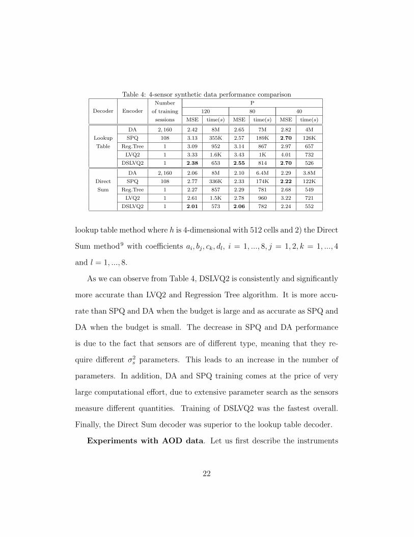
Table 4: 4-sensor synthetic data performance comparison
Decoder Encoder
Number P
of training 120 80 40
sessions MSE time(s) MSE time(s) MSE time(s)
DA 2, 160 2.42 8M 2.65 7M 2.82 4M
Lookup SPQ 108 3.13 355K 2.57 189K 2.70 126K
Table Reg.Tree 1 3.09 952 3.14 867 2.97 657
LVQ2 1 3.33 1.6K 3.43 1K 4.01 732
DSLVQ2 1 2.38 653 2.55 814 2.70 526
DA 2, 160 2.06 8M 2.10 6.4M 2.29 3.8M
Direct SPQ 108 2.77 336K 2.33 174K 2.22 122K
Sum Reg.Tree 1 2.27 857 2.29 781 2.68 549
LVQ2 1 2.61 1.5K 2.78 960 3.22 721
DSLVQ2 1 2.01 573 2.06 782 2.24 552
lookup table method where h is 4-dimensional with 512 cells and 2) the Direct
Sum method9 with coefficients ai, bj, ck, dl, i = 1, ..., 8, j = 1, 2, k = 1, ..., 4
and l = 1, ..., 8.
As we can observe from Table 4, DSLVQ2 is consistently and significantly
more accurate than LVQ2 and Regression Tree algorithm. It is more accu-
rate than SPQ and DA when the budget is large and as accurate as SPQ and
DA when the budget is small. The decrease in SPQ and DA performance
is due to the fact that sensors are of different type, meaning that they re-
quire different σ2s parameters. This leads to an increase in the number of
parameters. In addition, DA and SPQ training comes at the price of very
large computational effort, due to extensive parameter search as the sensors
measure different quantities. Training of DSLVQ2 was the fastest overall.
Finally, the Direct Sum decoder was superior to the lookup table decoder.
Experiments with AOD data. Let us first describe the instruments
22

that were used for data collection, mainly AERONET and MODIS.
AERONET is a global network of highly accurate ground-based instru-
ments that observe aerosols. They are densely situated in industrialized areas
and sparsely located elsewhere. For our evaluation purposes we considered
37 AERONET instruments located in North America15.
MODIS, aboard NASA’s Terra and Aqua satellites, is an instrument for
satellite-based AOD retrieval16 that provides global coverage with a moder-
ately accurate AOD retrieval estimated from multispectral images collected
by MODIS.
The characteristics of MODIS- and AERONET-based AOD retrieval are
quite different. AERONET retrievals consist of providing a single continu-
ous measurement (AOD retrieval) many times a day but only at instrument
location. On the other hand MODIS achieves an almost complete global cov-
erage daily, providing multivariate observations extracted from multispectral
images (e.g. reflectance, azimuth, etc.) in form of a feature vector that
serves as an input to NASA’s currently operational MODIS retrieval algo-
rithm (C005)17. C005 provides AOD retrieval predictions that are considered
to be of moderate accuracy. It is typically outperformed by more sophisti-
cated methods such as neural networks18,19.
Data collected using AERONET served as our ground truth y measure-
ment, while MODIS measurements at distributed locations collocated with
the corresponding AERONET site served as our x measurements. The collo-
cation of the AERONET and the MODIS data involved aggregating MODIS
23

observations into blocks of 10 km × 10 km around each AERONET site. In
our setup, 9 closest blocks to each AERONET site were considered, i.e. 9
21-dimensional feature vectors, x1,x2, ...,x9. The features constructed using
MODIS observations are said to be temporally collocated with the corre-
sponding AERONET AOD retrievals if there is a valid AERONET AOD
retrieval within a one-hour window centered at the satellite overpass time.
The data collocated in this way are obtained from the official MODIS Web
site of NASA17.
The goal was to design 9 encoders with M = 4 codewords aboard satellite,
and a decoder to be used at any ground location. Once the encoders and
the decoder are trained, the satellite no longer needs to transmit 9 × 21
continuous measurements for AOD prediction at specific ground locations.
Instead, only 9 discrete variables with cardinality M = 4 are communicated.
For our study, we collected 2, 210 collocated observations distributed over
37 North America AERONET sites during year 2005. A total of 1, 694 ex-
amples at randomly selected 28 AERONET sites were used as training data,
while 516 examples at remaining 9 AERONET sites were used as test data.
This procedure ensured that the resulting model was tested at AERONET
locations unobserved during training, which gave us some insight into model
performance at any North America ground location.
Table 5 compares prototype-based and regression tree algorithms in terms
24
of MSE and R2, defined as
R2 = 1−
N∑i=1
(yi − h(α1(x1i), α2(x2i)))2
N∑i=1
(yi − y)2
, (15)
where y = 1N
N∑i=1
yi.
Budget was set to P = 100, and estimation of y was made using the Di-
rect Sum fusion function h. Alternative fusion function lookup table method
was highly inefficient due to large number of table cells. The decentralized
estimation results were in addition compared to C005 and Neural Network al-
gorithms that used original features in absence of communication constraints.
A Neural Networks with 5 hidden layers was trained using resilient propaga-
tion optimization algorithm for 300 epochs.
It can be observed that DSLVQ2 outperformed the competing methods.
Using additional parameters in SPQ and DA was not beneficial, probably
due to large number of sources. Very low values of AOD retrievals might
also have effected the accuracy of SPQ and DA (y had a mean value of 0.14
and ranged from 0.006 to 1).
In addition, DSLVQ2 had better accuracy than NASA’s C005 algorithm
and performed fairly close to NN, while achieving significant communication
cost savings. Each satellite message for a single ground location requires
9×2 bits with DSLVQ2, requires 9×504 bits with NN, which is a significant
difference, especially when we consider that these measurements are taken
25

Table 5: 3× 3 grid AOD data performance comparison, Decoder: Direct Sum, M = 4
Data Type Algorithm
Number
of training MSE R2
sessions
Original Neural Network 10 .0058 .7952
Data C005 1 .0094 .6698
DA 256 .0098 .6564
Encoded SPQ 16 .0087 .6949
Data Reg.Tree 1 .0111 .6097
LVQ2 1 .0187 .3443
DSLVQ2 1 .0075 .7370
all year round.
5. Discussion
Overall, the most appealing features of DSLVQ2 are ease of implemen-
tation, training speed, and insensitivity to parameter selection. DSLVQ2
training is much faster than DA and SPQ because it does not require an-
nealing. On the accuracy side, DSLVQ2 is superior to LVQ2 and Regression
Trees, it is comparable to more expensive and difficult to tune SPQ and DA
algorithms in scenarios with small number of sensors, while it becomes supe-
rior to SPQ and DA when the number of sensors and sensor measurements
increases.
6. Conclusion
In this paper we addressed the problem of data-driven quantizer design in
decentralized estimation. We proposed DSLVQ2, a simple algorithm that was
shown to be successful in multi-type, multi-sensor environments. DSLVQ2
26
exhibits better performance than previously proposed LVQ2 and Regression
Tree algorithm. It also outperforms the state of the art DA algorithm in
applications with large number of sensors and sensor measurements, while
being less sensitive to parameter selection and orders of magnitude cheaper
to train.
References
1. Nguyen XL, Wainwright MJ, Jordan MI. Nonparametric Decentralized
Detection Using Kernel Methods. IEEE Transactions On Signal Pro-
cessing 2005;53(11):4054–4066.
2. Xiao JJ, Luo ZQ. Universal Decentralized Detection in a Bandwidth-
Constrained Sensor Network. IEEE Transactions on Signal Processing
2005;53 (8):2617–2624.
3. Lam WM, Reibman AR. Design of Quantizers for Decentralized Estima-
tion Systems. IEEE Transactions on Communications 1993;41(11):1602
–1605.
4. Fang J, Li H. Distributed Estimation of GaussMarkov Random Fields
With One-Bit Quantized Data. IEEE Signal Processing Letters 2010;17
(5):449 – 452.
5. Xiao JJ, Cui S, Luo ZQ, Goldsmith AJ. Linear Coherent Decentralized
Estimation. IEEE Transactions on Signal Processing 2008;56 (2):757–
770.
27
6. Grbovic M, Vucetic S. Decentralized Estimation using Learning Vector
Quantization. Data Compression Conference 2009;:446.
7. Megalooikonomou V, Yesha Y. Quantizer design for distributed estima-
tion with communication constraints and unknown observation statis-
tics. IEEE Transactions on Communications 2000;48(2).
8. Rao A, Miller D, Rose K, Gersho A. A generalized VQ method for com-
bined compression and estimation. International Conference on Acous-
tics Speech and Signal Processing 1996;:2032–2035.
9. Gubner JA. Distributed estimation and quantization. IEEE Transac-
tions on Information Theory 1993;39 (3):1456–1459.
10. Li H. Distributed Adaptive Quantization and Estimation for Wireless
Sensor Networks. Signal Processing Letters 2007;14 (10).
11. Wang TY, Chang LY, Chen PY. Collaborative sensor-fault detection
scheme for robust distributed estimation in sensor networks. Transac-
tions on Communications 2009;57 (10):3045 – 3058.
12. Kohonen T. The Self-organizing Map. Proceedings of the IEEE
1990;78:1464–1480.
13. Seo S, Bode M, Obermayer K. Soft nearest prototype classification.
Transactions on Neural Networks 2003;14:390–398.
28
14. MacQueen JB. Some methods for classification and analysis of multi-
variate observations. Proceedings of 5-th Berkeley Symposium on Math-
ematical Statistics and Probability 1967;:281–297.
15. Holben BN, Eck TF, Slutsker I, Tanr D, Buis JP, Setzer A, Vermote
E, Reagan JA, Kaufman YJ, Nakajima T, Lavenu F, Jankowiak I,
Smirnov A. AERONET: A federated instrument network and data
archive for aerosol characterization. Remote Sensing of Environment
1998;66 (1):116.
16. Kaufman Y, Menzel WP, Tanre D. Remote sensing of cloud, aerosol,
and water vapor properties from the Moderate Resolution Imaging Spec-
trometer (MODIS). IEEE Transactions on Geoscience and Remote
Sensing 1992;30 (1):2 – 27.
17. Remer LA, Tanr D, Kaufman YJ, Levy R, Mattoo S. Algorithm for
remote sensing of tropospheric aerosol from MODIS: Collection 005.
MODIS Algorithm Theoretical Basis Document ATBDMOD-04 2006;.
18. Radosavljevic V, Vucetic S, Obradovic Z. A Data-Mining Technique for
Aerosol Retrieval Across Multiple Accuracy Measures. IEEE Geoscience
and Remote Sensing Letters 2010;7 (2):411–415.
19. Ristovski K, Vucetic S, Obradovic Z. Uncertainty analysis of neural
network-based aerosol retrieval. IEEE Transactions on Geoscience and
Remote Sensing 2012;50 (2):409–414.
29