Decentralized, Modular Real-Time Control

for Machining Applications∗

John Yook, Dawn Tilbury,

Kalyani Chervela*, Nandit Soparkar*

The University of Michigan

Mechanical Engineering and Applied Mechanics

*Electrical Engineering and Computer Science

Ann Arbor, MI 48109

{jyook,tilbury,kvc,soparkar}@umich.edu

September 25, 1997

Abstract

In order to realize the vision of reconfigurable manufacturing systems, the machine tool hardware, as

well as the software which controls it, must be constructed in a modular fashion. We envision that each

hardware module, be it a single spindle, linear or rotary axis, or a multi-axis grouping, will have its own

sensors as well as control hardware and software modules. When a set of modules are grouped together

to form a machine, the control task may demand not only certain requirements for individual axes, but

also have constraints on the coordination of interacting axes (as in a contouring application). Thus,

the axis-level control modules, running on distributed processors with communication over a network,

must be coordinated in an appropriate way to ensure that the desired task is completed with the highest

possible speed and accuracy. This coordination gives rise to stringent constraints on both the control

execution as well as the data communication between control modules.

In this paper, we investigate several different architectures for a distributed control system for a

reconfigurable machining system. We describe how the control requirements for a manufacturing control

system map to temporal constraints on the data managed for the environment. We show how the various

time delays associated with distributed architectures impact the performance of the control algorithms,

and describe different types of communication protocols that can be implemented to meet the required

deadlines.

1 Introduction

Currently, the commercially-available control systems for machine tools are not reconfigurable. Modularcontrol systems are being investigated at several research locations, but to our knowledge, few addressdirectly the coordination problems among control processes running in a distributed environment.

Although control theorists traditionally consider algorithm development, at some point the algorithmsmust be converted into software which can run on one or more computers. The analysis and design ofdistributed real-time control systems in a modular heterogeneous environment requires the study and inte-gration of two complementary areas:∗This research was supported in part by the NSF Engineering Research Center for Reconfigurable Machining Systems at the

University of Michigan.

1

• development of modular, decentralized, reconfigurable real-time control strategies — i.e, an area withincontrol systems.

• design and implementation of modular, distributed real-time coordination software, on heterogeneousplatforms — i.e., an area under computer software systems.

Within this research area, we are looking at some of the issues in real-time and distributed implemen-tation of control algorithms for machine tools. Once a modular control system has been designed, andthe interaction between control modules specified, there are many different ways in which the control mod-ules can be mapped to a hardware implementation. A multi-processor architecture is also modular froma hardware perspective, and can be more reconfigurable than a single-processor control system. However,the communication overhead associated with a multi-processor system may impact the control performancesignificantly. We are especially interested in evaluating the performance of decentralized control systems, inwhich there is no centralized scheduler, to increase modularity. As processors become more powerful andand networks become faster, this type of control architecture has the potential to be both high-performanceas well as modular and reconfigurable.

In this paper, we investigate several different architectures for a control system for a reconfigurablemachining system. The delays inherent in these different types of control systems are enumerated andtheir effects on the system performance evaluated. We show how the various time delays associated withdistributed architectures impact the performance of the control algorithms, and describe different types ofcommunication protocols that could be implemented to meet the required deadlines. In addition, a two-axis contouring system is considered in some detail, and the effects of various delays on the contour errorare determined by simulation. These analytic and simulation results can be used to specify the maximumallowable communication delays in the system. These control requirements for a manufacturing controlsystem can be mapped to temporal constraints on the data managed for the environment.

1.1 Reconfigurable machining systems

The overall goal of the Engineering Research Center for Reconfigurable Machining Systems at the Universityof Michigan is to develop the necessary theory and technology to enable the next generation of machiningsystems to be quickly and easily reconfigured in response to changing market demands and new technologyinnovation [15]. One important facet of this vision is a reconfigurable control system. Such a system must beeasy to design and must be composed of standard modules (hardware and software) that are interchangeableand extensible. It must be upgradable, so that new sensors and control algorithms can be added to existingsystems.

Currently, most manufacturing systems are controlled using NCs, CNCs, and PLCs — which are relativelyinflexible. The trend is toward using the more flexible PC-based systems for such control. Furthermore, toallow for modularity and distribution, the aim is to allow automated generation of, say, C code given thecontrol specification for a particular configuration. At present, such automated code generation is primarilyfor centralized computing units.

In order to design and build modular controllers for modular machine tools, the issue of modularity itselfmust first be examined. It must be understood how different control algorithms should modularized (what isthe appropriate granularity) and how they should be combined. In this paper, we assume that the modulesare defined according to their purposes: position servo, cross-coupling, process control, etc. We consider theissues of how the control algorithm modules should be allocated among the many processors and how thecommunication between processors should be scheduled; we also discuss the performance tradeoffs associatedwith the different choices.

Decentralized control architectures are desirable for reconfigurable machining systems. Each machinemodule can have its own control module, complete with sensors, microprocessors, and a network connection.

2

As the mechanical modules are fitted together to create a fully functional machine, so will the controlmodules be linked together over the network to create a fully functional control architecture. Although thedecentralization has the advantages of simplicity and modularity, the communication delays over the networkcan lead to decreased stability and performance of the overall system.

1.2 Machine tool control

Our focus is on machining operations which are accomplished through the relative motion of a tool and theworkpiece. We consider a contouring machining system as an example (though the techniques which wedevelop may be generalized). In contouring systems, the cutting occurs as the axes of motion are moved(e.g., as in a milling machine). The axes of motion may move simultaneously, each at a different velocity.

The two major performance criteria for machining operations which we will consider are productivity andaccuracy. To achieve higher productivity (measured by the number of parts made over a given time period),the machine tool must move quickly with respect to the workpiece. This high feed-rate may decrease theaccuracy of the produced parts. The most desirable balance between productivity and accuracy is chosenwhen the part program is written. Advanced control techniques which can increase the feed-rate withoutdecreasing the accuracy are desirable, but due to the closed architecture, cannot be implemented withincurrent commercially-available machine tool control systems.

The accuracy of a machine tool is often described in terms of the axis errors and the contour errors (i.e.,various deviations from the precisely required trajectories). While in a machining system there are manysources of errors, in this work we focus on the errors associated with real-time, distributed communicationand computation. We consider different controller architectures and the impact of these types of errors onthe performance of the data and coordination of control system. Therefore, we assume that there are noerrors associated with imperfect modeling of the axis motions, and no disturbances such as electrical noise,thermal deformation, or sensor inaccuracies associated with the machine.

1.3 Data management

The interactions between the control system and the manufacturing environment, involving large quantitiesof real-time sensor, actuator and control data, need to be managed correctly and efficiently. The states of themachine tools, the sensor readings, actuator signals, and control variables, all together represent the data tobe managed. The various manufacturing activities that take place are coordinated in real-time, and in turn,they impose certain consistency and temporal constraints on the managed data. Yet, it is also necessary toallow autonomous executions in the distributed environment to allow for modularity and reconfigurability.Below, we describe the target domain in more detail in order to explain how the constraints arise in thispractical domain.

The current approach to designing and developing machine control in manufacturing is a very labor-intensive process. It usually involves developing all the application software, even though much of the codeis similar to that written for other applications. The code execution is timed in an ad hoc manner, andexperiments are run to check if the code can satisfy the real-time requirements of manufacturing. Thissoftware development process requires considerable effort, is very costly, and often takes several months. Ifthe manufacturing requirements are changed, the code must be re-developed, and experiments done again toverify that the new code works correctly. Such issues are common in the development of real-time computingsoftware (e.g., see [23]). To alleviate these problems in the context of reconfigurable manufacturing, we areinvestigating real-time data and coordination control strategies that are expected to run on commerciallyavailable computing platforms. Our research on the software for distributed coordination protocols hasidentified the coordination constraints in manufacturing systems that need support from a computing system.We propose imposing coordination constraints using a distributed database of the associated data, and

3

associated temporal constraints among the data. Thereafter, we consider Quality of Service (QoS) issues interms of meeting the real-time requirements for data management. The data includes sensor, actuator, andreference coordination data.

1.4 Related work

There are currently several related real-time control and coordination efforts at varying stages of developmentand deployment; a more detailed literature review can be found in [25].

1.4.1 Machine-tool control architectures

The Robotool is a 5-axis milling machine at University of Michigan with a first generation object-orientedopen architecture controller [13]. This object-oriented modular programming architecture can simplify thewriting of control programs. Robotool is a good attempt at creating modular controllers. There is somesupport for meeting real-time requirements, and some support for using multiple processors. However, theeffort is not directed toward decentralized control of machine tools (the control is centrally scheduled), leavingunexamined most of the issues related to decentralized real-time control.

In the context of the Robotool, Koren et al. describe the effect of timing issues on an open-architecturemachining system [13, 14]. They consider the four basic types of control that must be performed on a singlemachine tool:

1. adaptive compensation and event management

2. interpolation

3. servo control

4. emergency control

and determine the minimum sampling time as the sum of the execution times of each type of control. Betterperformance can be achieved using a hierarchical controller with different sampling times for each of thethree levels of control (this allows the servo control, the most critical, to execute more frequently). However,even in the hierarchical framework, it is difficult to reconfigure the control, because if a new axis were tobe added, all the sample times must be recomputed. A multi-processor architecture could alleviate manyof these problems; a real-time network would be necessary to allow communication amongst the variousprocessors.

Altintas et al. [1, 2] have proposed a modular design for a CNC. They use a hierarchical architecture withtwo buses: the main (ISA) bus and the CNC bus. On the main bus, there are several processor boards, eachdedicated to a specific machine tool monitoring or control task (such as data acquisition, chatter detectionand suppression, force control). The number of boards that can be added is constrained by the number ofphysically-available ISA slots. One of these processor boards is designated as the CNC master; it performsthe interpolation as well as the real-time job management for the axis-level controllers. ManufacturingAutomation Laboratories [19] has commercialized many of these technologies. The timing issues associatedwith this architecture have not been fully examined.

1.4.2 Fieldbus-based systems

Decotignie et al. describe an integrated communication and control system in [3]. They analyze the delaysassociated with communication over a fieldbus for both parallel and sequential computation at the distributedprocessors. The computations are assumed to be synchronized over the network with a unknown period, anda processor will only initiate a computation if all the necessary inputs from its predecessors are available.

4

Both feedforward (interpolator) and feedback (servo) control strategies are considered, and the (perhapsobvious) conclusion is drawn that a higher number of axes can be handled if the fieldbus is placed betweenthe interpolator and the axis control loops than if the axis control loops are closed over the fieldbus.

Song et al. also describe a distributed control architecture over a fieldbus [20]. They describe a multi-axis machine-tool with one processor for the central control (in their example, interpolation) plus anotherprocessor for each axis servo control. Synchronization between axes is done by time-synchronizing the axiscommands over the real-time network.

They describe the distribution of a control system by three steps: the functional architecture, the hard-ware architecture (processors and networks), and the operational architecture (which is mapping the func-tional definition onto the chosen hardware). They briefly describe the Structured Analysis and DesignTechnique which breaks the functionality down into a set of elementary data processing modules calleddistribution atoms which can neither be distributed on several nodes nor partly executed. However, theynote that the description formalism is not yet fully defined. Also, no formal methods exist for optimallydistributing these atoms onto a hardware architecture.

Ferrarini et al. [4] have looked at hybrid position and force control for an industrial robot; they enableforce control when contact is made, and turn it off when contact is broken. Their control is implemented ina distributed environment. In essence, they have reconfigured their system by adding an extra CPU boardto an existing architecture to handle the added force control functions.

1.4.3 Other real-time control efforts

Onika is an on-going project at Carnegie-Mellon University which was built to implement real-time controllersfor robots [6]. Onika has a multilevel human-machine interface for real-time sensor-based systems. The upper-level provides a user-friendly interface to combine different control objects. The middle-level has the actualcode associated with the control objects. Finally, the device drivers and sensor interfaces are in the lowestlevel. These layers are built on top of a proprietary real-time operating system. Control modules executeon multiple processors, and communication between them is managed through shared memory. However, itdoes not address real-time communication between control modules which do not share a common bus. Ithas little support for Quality of Service trade-offs between quality and performance.

Wittenmark et al. [27] give a brief overview of some timing problems in real-time control systems. Theyenumerate three types of problems: control delay (the elapsed time between sensing and actuation), jitter(time-variation in start time of actions), and transient errors (due to loss or corruption of control-relatedsignals during communication). They show, through simulation, how delays can affect performance. Theinverse problem, that of specifying the maximum allowable delay given a specified performance criteria,remains unsolved.

2 Machine tool control structure

Following Koren et al. [13], in this paper we consider three basic types of control modules for a multi-axismachine tool controller: servo, interpolation, and process. Emergency control will not be considered here.

2.1 Servo control

First we consider the axis-level controllers, also called servo controllers. In an effort to simplify the problem,in order to highlight the effects of communication and computation delays, we model each axis of a machinetool as a simple second-order transfer function P (s).

P (s) =X(s)V (s)

=K

s(s+ a)(1)

5

More precise models can be found in [11, 12, 8].Typically, each axis will have its own servo controller to allow it to track reference inputs. Servo controller

operates in discrete-time with a sampling time of Ts. A proportional-integral (PI) control law gives a closed-loop axis system of Type II, allowing ramp reference inputs to be tracked with zero steady-state error. Thecontinuous-time transfer function of our PI controller is given by

C(s) = KP +KI

s(2)

and a discrete approximation to this continuous-time controller is constructed using the bilinear approxima-tion [5].

It has been shown that a slightly more complicated PID controller can improve the performance of thesystem [17], although most industrial machine tool controllers use the simpler PI algorithm [26]. Again,we have chosen to use simple models for our preliminary study to highlight the effects of the delays in thesystem. One potential reconfiguration of a machine tool system would be to upgrade some (or all) of theservo controllers from PD to PID. Another potential upgrade would be to add friction compensation to theservo-level controllers to decrease the errors due to stiction effects [7, 8].

2.2 Interpolation

An interpolator coordinates the axes by decomposing the desired operation motions into individual axisreference commands [11]. The input to this module depends on the type of motion (such as linear, circular,or parabolic). However, the most basic inputs to this module are the initial and final positions of eachaxis and the desired feed-rate (the speed of the tool relative to the workpiece). Using this information,the interpolator generates the reference positions for each axis. In conventional machining operations, thedesired feed-rate for each motion is stored in the part program. Intelligent machining systems often adjustthe feed-rate in real-time to increase operation productivity and quality using adaptive process control (asdescribed in the following section).

2.3 Adaptive process control

Adaptive or process control can be used to optimize productivity and accuracy [16]. Even though there arenumerous types of process control, most of them are implemented by adapting the desired feed-rate and/orpositions in response to external inputs or disturbances. For example, force control changes the feed-rate tomaintain a constant force on the tool; this can prevent tools from breaking and minimize tool wear. Chattersuppression can be done by either decreasing the spindle rotational speed or decreasing the depth of cut;newer results show that varying the spindle speed sinusoidally can also help to reduce chatter [28]. Thermaland geometric compensators change the initial and final value to the interpolator to account for the thermalexpansion or known geometric inaccuracies in the machine tool.

Adaptive control algorithms may operate at a different sampling time than the servo controls. Becausethey act by modifying the reference inputs to the servo controller (either directly or indirectly throughthe interpolator), this sample time is usually longer than the sample time of the servo controller but isnever shorter (it may be the same). In contrast, the computation time associated with an adaptive controlalgorithm is often longer than that associated with a servo controller.

Adaptive control algorithms may require the knowledge of many sensor inputs (such as positions, forces,temperatures, etc.). This data may be transmitted over a network, causing communication delays which canaffect the performance of the adaptive control algorithms.

6

2.4 Cross-coupled control

A cross-coupled controller can improve the contouring accuracy (independent of the tracking accuracy ofeach axis) in a two-axis machine tool system [10, 22]. The cross-coupled control module coordinates themotion of the two axes to minimize the contour error. It takes as inputs both the x and y references andsensed positions, and computes the distance between the actual (x, y) position and the desired contour. Ituses this difference to either compute appropriate control voltages for both the x and y axes to add to theoutputs of the servo controllers, or to send a signal to the interpolator which then modifies the referencevalues to the servo controllers. Thus, a cross-coupled controller can be considered either as part of the servoloop (if its action is to modify the commanded voltages to the motors) or as part of the adaptive processcontrol (if its action is to modify the commanded references to the servos).

There are two major parts in the cross-coupled control algorithm: the estimation of the contour error andthe design of cross-coupled compensator. To estimate the contour error, the cross-coupled control algorithmneeds measurements of the actual position of x and y as well as the reference inputs. The number of datapoints needed from each subsystem is determined by the desired accuracy of the contour error estimation.The contour error can be estimated by [22]

εx = (sin2 θ)ex − (cos θ sin θ)ey (3)

εy = (cos2 θ)ey − (cos θ sin θ)ex (4)

where θ is the instantaneous inclination of the tangent to the contour path. For the cross-coupled compen-sator, a simple gain controller will suffice [10, 22] although more complex control laws may give even betterperformance.

The steady state value of the contour error is highly dependent upon the overall gain of the cross-couplingcontroller. Larger values of the cross-coupled gain result in decreasing contour error; however, if the gain istoo high, the system can become unstable (as shown in Section 4.4).

2.5 Example: A two-axis contouring system

The main example that we will use in this paper is a simple two-axis milling machine for contouring applica-tions. The milling machine has a vertical (z-axis) spindle on which the tool is mounted, and an x-y table toposition the metal underneath the mill. For simplicity, we assume that the position of the spindle is fixed;we only consider the motion of the x-y table. For this example, we will examine the effects of delays onthe performance of a servo and cross-coupled control system; process control algorithms are currently underinvestigation.

Let the x-y table trajectories be (rx(t), ry(t)), and the actual sensed positions be (x(t), y(t)). We assumethat the reference trajectory is a circle with center (xc, yc) and radius R, hence:

(rx(t), ry(t)) = (xc +R sin(t), yc +R cos(t))

In a contouring system, the control performance criterion is given by the contour error. The contour error(ε) is defined as the shortest distance from (x, y) to the desired circle:

ε(t) =√

(x(t)− xc)2 + (y(t)− yc)2 −R

which is not the same as√e2x + e2

y.

We will use a cross-coupled controller which estimates the contour error using equations (3)–(4) andcompensates for it using a constant gain W (we assume Wx = Wy = W ).

7

3 Computing and communication architectures for control

The performance of a distributed control system is determined not only by the control algorithm but also bythe computing and communication architecture with which the algorithm is implemented. Both computationand communication delays occur in a distributed system, and their effects must be considered. In general, agiven control algorithm could be implemented in many different ways, with different numbers of processorsand different communication networks.

In this section, we define four different architectures for machine tool control and examine the advantagesand disadvantages of each architecture in terms of reconfigurability and expected performance. For each ofthe several different types of architectures, we will discuss the types of delays that occur. The effect of thesedelays on the transient and steady-state performance of the system will be analyzed in the following section.Because we are interested in designing control systems for reconfigurable manufacturing systems, we alsobriefly discuss the ease with which different configurations can be reconfigured or upgraded on an as-neededbasis.

3.1 Sources of delay

The two main sources of delay in a control system are the communication delay associated with sendinginformation over a network, and the computation delay associated with computing control algorithms on amicroprocessor. In Figure 1, we have shown a simple block diagram of a control system and noted severallocations where time delays can occur. A delay in between the servo controller and the plant is caused bythe computation time needed to compute the servo control algorithm and is denoted TCP . A sensing delayfrom the output of the plant back to the servo controller is denoted TPC . A delay between the interpolatorand the reference input to the servo controller, due to communication delays, is denoted TRC . In the eventthat adaptive process control is contained in the loop, there could be sensing delays to the controller TPAas well as communication and computation delays between the adaptive control block and the interpolator,which are lumped together as TAR. Even though there will be only one sensor per state, two different delays(TPC and TPA) are shown in Figure 1 to represent the fact that the time required for the sensed data toreach the different control blocks depends on both the network and the system architecture.

3.2 Centralized architecture

We define a centralized control architecture as a single block which computes the control commands to allthe actuators of the system and has complete knowledge of the state of the entire system. It is typicallydesigned around a complete multi-variable model of the plant, and uses the position sensor data from allaxes. This large block may also contain the interpolator, or it may compute the reference values separately.

A conventional multi-variable controller would be one example of an architecture which fits into thiscategory. Since a centralized control algorithm has complete knowledge of the system, and can compensatefor coupling between axes through the multi-variable system model, it has the best possible performance ofall the control design architectures. In order to achieve this level of performance, however, the centralizedcontroller must be implemented on a single processor with negligible computation and sensing delays. Thisis certainly possible for systems with one or two axes, but becomes more difficult for many degree-of-freedommachines. In addition, as the number of axes (and states) increases, the modeling and control designprocedures become more complex. More complicated control algorithms are needed, which may increase thecomputational delay to unacceptable levels.

A centralized control architecture is not considered to be reconfigurable. If the machine is updated tohave extra (or fewer) axes, or if a change in the control algorithm is desired, the entire system model must

8

INTERPOLATOR

e-TPA S

SERVOPLANT

ADAPTIVEPROCESS

CONTROLLER

CONTROLLERe-TAR S

e-TCP S

e-TPC S

e-TRC S

Figure 1: A simple two-loop control system with a servo controller, interpolator, and adaptive processcontroller, showing the possible delays in the loops. A delay in between the servo controller and the plant,caused by the time needed to compute the servo control algorithm, is denoted TCP . A sensing delay fromthe output of the plant back to the servo controller is denoted TPC . The delay between the interpolator andthe reference input to the servo controller, due to communication delays on the network, is denoted TRC .In the event that adaptive process control is contained in the loop, there could be sensing delays to thecontroller TPA as well as communication and computation delays between the adaptive control block andthe interpolator, which are lumped together as TAR.

be rebuilt and the controller redesigned. Although some automated techniques exist to assist in these steps,the process is still time-consuming and hence expensive.

Although a centralized control architecture is usually implemented on a single processor, a multi-processorsystem with a centralized scheduler may be implemented if the control is too complex for the availablehardware to handle in the required sample time. We still consider this architecture to be centralized andnot reconfigurable.

3.3 Decoupled architecture

The other extreme from a centralized architecture is a decoupled architecture. We define a control systemto be decoupled if each actuated degree of freedom has its own control block with only local knowledge ofthe sensed outputs. For example, if each actuated axis has a sensor and a servo controller, but there is nocommunication among the servos, the control system would be called decoupled. As the name implies, adecoupled control architecture cannot compensate for coupling among the degrees of freedom. In a machiningapplication, there will still be a central interpolator which generates the desired trajectories for all axes.

Although a decoupled control architecture could be implemented on a single processor, the structurenaturally lends itself to distribution amongst many processors. This type of distributed multi-processorstructure can decrease the magnitude of both the communication and computation delays. For example, ifeach axis has its own processor and sensor, and the only tasks that the processor must perform are readingthe sensor value and computing the servo algorithm, the time delays involved will be relatively small. Therewill still be a network connection to communicate the reference value for the servo controller, but the sensordata does not need to be communicated across any sort of network. A single-axis servo control algorithm istypically quite simple and does not require extensive computation time.

Because of the minimal communication and computation delays, a decoupled control architecture cansupport a small servo-level sampling time, potentially increasing the accuracy of the axis-level positioning.Such a system may still have significant contour errors. In addition, a decoupled control architecture iseasily reconfigured; when an axis is added to or removed from the system, only the interpolator needs to be

9

reprogrammed.

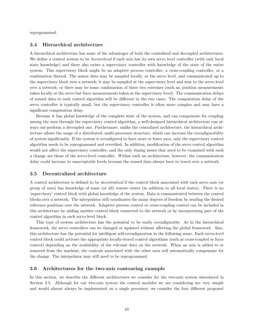
3.4 Hierarchical architecture

A hierarchical architecture has some of the advantages of both the centralized and decoupled architectures.We define a control system to be hierarchical if each axis has its own servo level controller (with only localstate knowledge) and there also exists a supervisory controller with knowledge of the state of the entiresystem. This supervisory block might be an adaptive process controller, a cross-coupling controller, or acombination thereof. The sensor data may be sampled locally, at the servo level, and communicated up tothe supervisory block over a network; it may be sampled at the supervisory level and sent to the servo levelover a network; or there may be some combination of these two extremes (such as, position measurementstaken locally at the servo but force measurements taken at the supervisory level). The communication delaysof sensed data to each control algorithm will be different in the two cases. The computation delay of theservo controller is typically small, but the supervisory controller is often more complex and may have asignificant computation delay.

Because it has global knowledge of the complete state of the system, and can compensate for couplingamong the axes through the supervisory control algorithm, a well-designed hierarchical architecture can al-ways out-perform a decoupled one. Furthermore, unlike the centralized architecture, the hierarchical archi-tecture allows the usage of a distributed, multi-processor structure, which can increase the reconfigurabilityof system significantly. If the system is reconfigured to have more or fewer axes, only the supervisory controlalgorithm needs to be reprogrammed and reverified. In addition, modification of the servo control algorithmwould not affect the supervisory controller, and the only timing issues that need to be examined with sucha change are those of the servo-level controller. Within such an architecture, however, the communicationdelay could increase to unacceptable levels because the sensed data always have to travel over a network.

3.5 Decentralized architecture

A control architecture is defined to be decentralized if the control block associated with each servo axis (orgroup of axes) has knowledge of some (or all) remote states (in addition to all local states). There is no‘supervisory’ control block with global knowledge of the system. Data is communicated between the controlblocks over a network. The interpolator still coordinates the many degrees of freedom by sending the desiredreference positions over the network. Adaptive process control or cross-coupling control can be included inthis architecture by adding another control block connected to the network or by incorporating part of thecontrol algorithm in each servo-level block.

This type of system architecture has the potential to be easily reconfigurable. As in the hierarchicalframework, the servo controllers can be changed or updated without affecting the global framework. Also,this architecture has the potential for intelligent self-reconfiguration in the following sense. Each servo-levelcontrol block could activate the appropriate locally-stored control algorithms (such as cross-coupled or forcecontrol) depending on the availability of the relevant data on the network. When an axis is added to orremoved from the machine, the controls associated with the other axes will automatically compensate forthe change. The interpolator may still need to be reprogrammed.

3.6 Architectures for the two-axis contouring example

In this section, we describe the different architectures we consider for the two-axis system introduced inSection 2.5. Although for our two-axis system the control modules we are considering are very simpleand would almost always be implemented on a single processor, we consider the four different proposed

10

2 axis system with cross coupled controller

x ref

controller for x

−+

Sum

e_x nump_x(s)denp_x(s)

x axis

1

Outport

X++

Sum2

C/C controllerref. input y ref

nump_y(s)denp_y(s)

y axis

Y 2

Outport1controller for y

e_y

+−

Sum1

++

Sum3

y measured

x measured

ref. input.

ref. input

C/C controller

z1 communication

delay(Td)

z1 communication

delay(Td).

C/C controller.

data bank

data bank.

2 axis system with distributed cross coupled controller

+−

Sum10controller for y

−+

Sumcontroller for x

nump_x(s)denp_x(s)

x axis

2

Outport1

nump_y(s)denp_y(s)

y axis

1

Outport

X

a. Hierarchical b. Distributed

Figure 2: Simulink diagram of the cross-coupled controller. In each configuration, each axis has a servo-control module which is a simple PI controller. For the hierarchical implementation, there is a cross-couplingmodule which coordinates the motion of the two axes. For the distributed implementation, there is a cross-coupled control module for each axis.

architectures in order to study the communication requirements of the different types of controllers and theeffects of communication and computation delays on the control performance.

We consider four basic control architectures for the two-axis milling machine example; these are shownin Table 1. The two extremes are a centralized controller, in which there is no distributed processing, and adecoupled controller, in which there is no communication between the two axes. The decoupled controller isthe simplest type of control architecture, consisting only of the two servo-level control modules, but has theworst performance since the contour error is not considered and thus cannot be compensated. As noted above,the performance of a machine tool control system can be improved by using a cross-coupled controller. Thesame cross-coupled control algorithm can be implemented in two different ways: as a hierarchical controller,or in a decentralized (but coordinated) manner.

The control structure shown in Figure 2a is considered to be modular as compared to a centralizedcontroller (the first block in Table 1). There is a servo control module for each axis (x and y) in additionto the cross-coupling module. We also consider the cross-coupled controller in a distributed architecture asshown in Figure 2b. The distributed control increases the modularity of the system by having a cross-couplingcontrol module for each axis but does not change the nominal system performance (i.e., the control equationsremain unchanged). Different types of time delays will affect the system in each type of architecture; theeffects of these delays will be shown in Section 4.4.

4 Effects of computation and communication delays

In order to determine the best control system architecture for a reconfigurable machining system, we mustfirst understand the effects of communication and computation delays associated with the different archi-tectures. It is commonly known that delays in a control system tend to decrease performance and can evencause instability. Due to the nonlinearity associated with time delays, however, it may be difficult or evenimpossible to solve analytically for the effects of delays. In addition, if the system is reconfigured, and thecontrol structure or algorithms change, the analysis should be done again.

In this section, we present a combination of simulations and analysis to show how time delays can affectthe system’s performance. As might be expected, different types of time delays have different effects. Time

11

controller type advantages disadvantages

C(z)

P(s)

(DATA BANK)INTERPOLATOR

xref(t)yref(t)etc...

xref(t)yref(t)etc...

CENTRALIZED CONTROLLER

X

YP(s)best performance not reconfigurable

C(z) P(s)

C(z) P(s)

ƒ(x,y) ƒ(xref,yref)

CONTOURERROR

(DATA BANK)INTERPOLATOR

xref(t)yref(t)etc...

xref(t)yref(t)etc...

DECOUPLED CONTROLLER

X

Y

++

+ -

-

-

most reconfigurable poorest performance

C(z) P(s)

C(z) P(s)

(DA

TA

BA

NK

)IN

TE

RP

OLA

TO

R

xref(t)yref(t)etc...

xref(t)yref(t)etc...

CROSS COUPLED CONTROLLER

C/C controllercorection term

for ε(x,y,xref,yref)

X

Y

good performance communication delaysgood reconfigurability central process needed

C(z) P(s)

(DA

TA

BA

NK

)IN

TE

RP

OLA

TO

R

xref(t)yref(t)etc...

xref(t)yref(t)etc...

DISTRIBUTED CROSS-COUPLED CONTROLLER

+

+

-

-C/C controllercorection term

for ε(x,y,xref,yref)

communicationaldelay

C/C controllercorection term

for ε(x,y,xref,yref)

X

C(z) P(s)Y

good performance communication delaysgood reconfigurability

Table 1: Four different control architectures, and comparisons, for a two-axis milling machine: centralized,decoupled, hierarchical cross-coupled, and decentralized cross-coupled .

12

0 0.5 1 1.5 2 2.5 3

−0.02

−0.015

−0.01

−0.005

0

0.005

0.01

0.015

0.02

time; [sec]

erro

r ca

used

from

Trc

Error caused from input delay

Trc = 0.001 secTrc = 0.005 secTrc = 0.009 sec

0 0.5 1 1.5 2 2.5 3

−0.02

−0.015

−0.01

−0.005

0

0.005

0.01

0.015

0.02

time; [sec]

erro

r ca

used

from

Tcp

Error caused from computational delay

Tcp = 0.001 secTcp = 0.005 secTcp = 0.009 sec

0 0.5 1 1.5 2 2.5 3

−0.02

−0.015

−0.01

−0.005

0

0.005

0.01

0.015

0.02

time; [sec]

erro

r ca

used

from

Tpc

Error caused from sampling delay

Tpc = 0.001 secTpc = 0.005 secTpc = 0.009 sec

a. reference delay TRC b. computational delay TCP b. sensing delay TPC

Figure 3: Errors caused by time delays, comparing the effects of magnitude and location. The referencedelay TRC from the interpolator to servo controller, the computation delay TCP in the servo controller, andthe sensing delay TPC between the sensed outputs of the plant and the servo controller are considered. Foreach type of delay, three separate magnitudes (0.001, 0.005, and 0.009 sec) are considered. The samplingtime Ts of both the servo controller and the interpolator is 0.01 sec. The errors are expressed in terms ofthe difference between the outputs of the system with time delay and the system without delay; the inputto the system is a ramp with unit slope. Note that the maximum and the steady state errors depend notonly on the size of the delay but also the location of the delay.

delay tends to increase the maximum error as well as the average error, and may also change the steady stateerror of system. We will also show how certain combinations of time delays can actually result in improvedperformance over single time delays. We expect that this type of simulation and analytic information willbe useful not only in choosing the best type of system architecture, but also in designing the communicationprotocols that will be used in a reconfigurable machining system (as described in Section 5).

For this preliminary study, we have considered a single-axis, single-loop servo system with an interpolator.We analyzed the effects of the time delays shown in Figure 1 when the servo controller is a PI algorithm, theplant is a second-order motor, as described in Section 2.1, and the reference is a ramp function with unitslope.

The errors that we present in Figures 3 and 4 are all expressed as compared to the same system withoutany time delay. As shown in Figure 3, the effect of the time delay depends not only on the magnitude of thetime delay but also on its position in the control loop. The effects of the combination of different types oftime delays in the system are shown in Figure 4. Of particular interest is the fact that for this simple system,the errors due to the time delays are additive. Most notably, the positive and negative steady-state errorsassociated with the reference and sensing delays cancel. This indicates that if one of these types of delays isunavoidably present in the system, the system designer may compensate for it (at least in the steady-state)by intentionally introducing a delay on the other.

After we have described the effects of time delay in the single-loop system, we consider the two-axiscontouring system with cross-coupling control as described in Section 2.5. For this example, the closed-loopequations are nonlinear, and thus we have not done any analytic computations. In Section 4.4, the effectsof the sampling time of the two different control algorithms (servo and cross-coupled) as well as the effectdue to time delays in various parts of the loop will be discussed. The performance criterion for this systemis the contour error.

4.1 Analytic results

The modified Z-transform is an extension of the traditional Z transform which is useful in the study ofcombined differential and difference equations arising in the study of both hybrid (mixed continuous- and

13

0 0.5 1 1.5 2 2.5 3

−0.02

−0.015

−0.01

−0.005

0

0.005

0.01

0.015

0.02

time; [sec]

erro

r ca

used

from

Tpc

& T

cp

Error caused from Tpc & Tcp

Tpc & Tcp= 0.001 secTpc & Tcp= 0.005 secTpc & Tcp= 0.009 sec

0 0.5 1 1.5 2 2.5 3

−0.02

−0.015

−0.01

−0.005

0

0.005

0.01

0.015

0.02

time; [sec]

erro

r ca

used

from

Trc

& T

cp

Error caused from Trc & Tcp

Trc & Tcp= 0.001 secTrc & Tcp= 0.005 secTrc & Tcp= 0.009 sec

a. Computation delay TCP b. Computation delay TCPand sensing delay TPC and reference delay TRC

0 0.5 1 1.5 2 2.5 3

−0.02

−0.015

−0.01

−0.005

0

0.005

0.01

0.015

0.02

time; [sec]

erro

r ca

used

from

Tpc

& T

rc

Error caused from Tpc & Trc

Tpc & Trc = 0.001 secTpc & Trc= 0.005 sec Tpc & Trc= 0.009 sec

0 0.5 1 1.5 2 2.5 3

−0.02

−0.015

−0.01

−0.005

0

0.005

0.01

0.015

0.02

time; [sec]

erro

r ca

used

from

Tpc

& T

cp &

Trc

Error caused from Tpc & Tcp & Trc

Tpc & Tcp & Trc= 0.001 secTpc & Tcp & Trc= 0.005 secTpc & Tcp & Trc= 0.009 sec

c. Sensing delay TPC d. Computation TCP , sensing TPC ,and reference delay TRC and reference TRC delays

Figure 4: Here we show the effects of different combinations of delays. In each figure, three differentmagnitudes of delay are considered (0.001, 0.005, and 0.009 sec); the same magnitude is used for each typeof delay. The sampling time of the servo controller in all cases is Ts = 0.01 sec. The errors are expressed interms of the difference between the outputs of the system with time delay and the system without delay; theinput to the system is a ramp with unit slope. Of particular interest is the fact that for this simple system,the errors due to the time delays are additive. Most notably, the positive and negative steady-state errorsassociated with the reference and sensing delays cancel. This indicates that if one of these types of delays isunavoidably present in the system, the system designer may compensate for it (at least in the steady-state)by intentionally introducing a delay on the other.

14

discrete-time) systems and time delay systems. This analytic approach can be applied to obtain the valueof a function f(t) between the sample times as well as to compute the discrete transfer function of acontinuous system with time delay [5, 18]. Using this method, possible analytical error introduced byother methods (such as the Pade approximation) can be eliminated. Furthermore, the modified Z-transformhas the desirable properties of the standard Z-transform such as linearity, final value theorem, etc., greatlysimplifying the analysis of the system [18]. In this section, we describe how the modified Z-transform canbe used to analyze the closed-loop behavior of our example system with time delays.

Let the plant be a second-order type I system with transfer function

P (s) =K

s(s+ a)

For the examples we consider in this paper, this transfer function represents the motor of the machine toolas described in Section 2.1. The system with time delay λ can be expressed as

P ′(s) = e−λsP (s)

We will use the modified Z-transform to compute the exact output of the system at each sample time. Letthe delay λ be expressed in terms of the sampling period as

λ = (`−m) · Ts

where Ts is the sampling period , ` is an integer and m is a nonnegative number less than 1. If the delay isan exact multiple of the sample time, then m = 0.

The discrete transfer function P ′(z) of P ′(s) can be computed as follows. The main idea is to directlytake the Z-transform of the integral number of time delays (`) and then compute the time-shifts in the stepand exponential functions due to the fractional time-delay (m).

P ′(z) =z − 1zZ{e−(`−m)Tss · P (s)

s}

=z − 1z`+1

Z{e−ms · K

s2(s+ a)}

=K

a2

z − 1z`+1

Z{a(t+mTs)− 1 + e−a(t−mTs)}

=K

a2

z − 1z`+1

((amTs − 1)z

z − 1+

aTz

(z − 1)2+

e−amTs

z − e−aTs )

=K

a2

n1z2 + n2z + n3

z`(z2 − (1 + e−aTs)z + e−aTs)where

n1 = amTs − 1 + eamTs

n2 = (1− amTs)(1 + e−aTs) + aTs − 2eamTs

n3 = (amTs − 1)e−aTs − aTse−aTs + eamTs

This discrete transfer function P ′(z), used with the inverse of the modified Z-transform of the controller,enables us to find the error profile of the delay system [18].

4.2 Communication delays

We first consider the different types of communication delays that may be present in a system. The magnitudeof the delays will depend not only on the chosen architecture but also on the speed and configuration of the

15

chosen network. Some networks, such as Sercos, have fixed cycle times and deterministic operation. Others,such as Ethernet, are fast but can result in varying communication times. At present, our analysis onlyincludes fixed delay times; the effects of varying time-delays will be considered in future work.

4.2.1 Reference input delays

In any type of distributed system architecture (decoupled, hierarchical, or decentralized), the interpolatorwill send the reference values to the servo controllers over a network, resulting in a time delay. If the timedelay to all servos is the same, then the interpolator may operate in a “look-ahead” fashion to eliminatethe resulting errors. More complex compensation may be required when there are differing time delays todifferent axes, or the time delay may vary due to a nondeterministic network.

Consider a servo system as described in Section 2.1 with a ramp reference. A communication delay TRCbetween the interpolator and the servo controller will result in a steady state error of

ess = Vr TRC

Because the reference data reaches the servo controller after a delay of TRC , the steady-state error due tothe delay is equal to the reference velocity Vr times the time delay TRC .

This analysis holds true for a type I system with a PI servo controller (the closed-loop system is type II)and a ramp reference input with a slope of Vr. If the reference input were a step, then the steady-state errorfor the same controller and plant system would be zero for a reference input delay.

4.2.2 Sensing delays

Some or all of the sensed data may also be sent over a network. Some outputs (such as positions) are sampledat the highest frequency present in the system (usually the sample time of the servo loop). The minimumachievable sensing delay will depend on the amount of data that needs to be sent over the network (howmany outputs are sampled during each period), how often the data needs to be sent (the sample time), aswell as the bandwidth of the network. Of course, the network protocols and architecture will also influencethe amount of delay.

Using the final value theorem, we determine that a sensing delay TPC will result in a steady state errorof

ess = −Vr TPC

This result is analogous to the error caused by reference input delay. Because here the system output isdelayed in amount of TPC , the actual output will end up leading the reference, giving a negative error.

Again, we note that for the simple system we have considered, the effects of the sensing and referencedelays are additive. That is, the positive and negative steady-state errors associated with the reference andsensing delays cancel. This indicates that if one of these types of delays is unavoidably present in the system,the system designer may compensate for it (at least in the steady-state) by intentionally introducing a delayon the other.

Once again, this analysis holds true for a type I system with a PI servo controller (the closed-loop systemis type II) and a ramp reference input with a slope of Vr. If the reference input were a step, then thesteady-state error for the same controller and plant system would be zero for a reference input delay.

4.3 Computation delays

We also consider the delays associate with the finite computation time of the digital computer. We denotethis computation time as TCP . This delay depends not only on the complexity of control algorithm but alsoon the number of tasks a processor must complete during each sampling period. The effects of this delay

16

can be used to determine the number of processors that should be used in the system in order to meet agiven error specification. The control system designer should choose to allocate the tasks among multipleprocessors in the system in such a way as to minimize the effect of the computation delays.

The steady state value of the error caused by the computation delay is zero for the given system, eventhough the maximum overshoot error was increased as the magnitude of this delay increased (see Figure 3). Inaddition, the maximum overshoot error caused by this delay was less than the error from the communicationdelays TPC or TCP . Thus, we should choose the control architecture of the system in order to minimizethe communication delays as much as possible, even if that means increasing the computation delay byperforming many tasks on a single processor.

4.4 Simulation results for the two-axis contouring system

We simulated the cross-coupled controller with a circular reference input and several different control fre-quencies and communication frequencies. We varied both the frequency of the servo-level controllers Ts aswell as the frequency of the cross-coupled controller Tc. We also considered the effect of communicationdelays on the cross-coupled controller. We defined the performance measure of our control system as themaximum contour error and we computed this measure for several different scenarios.

The cross-coupled controller for the two-axis machine tool system was shown in Figure 2. Using blockdiagram reduction, the cross-coupled controller can be implemented in a decentralized fashion; this increasesthe modularity of the system without attenuating the nominal performance of the controller. Both thehierarchical and decentralized architectures are shown in the figure.

The results of our simulations are summarized in Figures 5–7. As shown in Figure 5, the maximum contourerror is an exponential function of the sampling time Ts. The frequency of the cross-coupled controller Tc alsoaffects the contour error, but its impact is highly dependent on the sampling time, Ts. For small samplingfrequencies (Ts < 0.03sec), the sampling frequency of the cross-coupled controller less than four times thesampling frequency have no significant effect on the contour error. However, the sampling frequency of C/Cwould dramatically increase the contour error as Ts is increased, its effects are much more significant thanthe delay associated with the communication. The effect of the communication delay between axes alsodepends strongly on the sampling time Ts (see Figure 6). In addition, the contour error depends stronglyon the cross-coupled gain W as shown in Figure 7.

We expect that simulation results such as these could be used as follows. For a given performancerequirement (such as maximum contour error), the sample times of the servo-level control Ts and the cross-coupled control Tc can be specified from the figures. The maximum allowable communication delay canalso be determined in a similar manner. The priority order of jobs can be specified as the following: firstis necessarily sampling and computing the servo-level control for each axis, then sampling and computingthe cross-coupled control algorithm for each axis, and finally data communication. In this manner, over-requirements on each task can be avoided, and if it is not possible to complete all tasks within a given timeinterval, the priority ordering is clear.

The sample times and communication requirements of the control algorithms will dictate the type andamount of computer hardware that will be required in the system, as well as the database structure andcommunication protocols that will be needed. Again, we emphasize that for this simple two-axis example,the performance requirements can be easily met with existing tools on a single processor. Machine toolperformance requirements continue to become more stringent, with very high speeds and very high (micron-level) accuracies. The next generation of machine tool controllers will require distributed computation andcommunication to achieve both the performance requirements and the desired reconfigurability.

17

0 0.01 0.02 0.03 0.04 0.05 0.06 0.07 0.08 0.09 0.10.025

0.03

0.035

0.04

0.045

Ts, sec

max

. con

tour

err

or, m

Sampling time(Ts) of the controller effects

1 1.5 2 2.5 3 3.5 4 4.5 50.025

0.03

0.035

0.04

0.045

sampling time of C/C controller, Tc: [Ts]

max

. con

tour

err

or, m

Sampling time(Tc) of C/C controller effects

Ts=0.01

Ts=0.03

Ts=0.05

Ts=0.07Ts=0.1

a. Effects of the sample time Ts b. Effects of the sample time Tcof the servo controller of the cross-coupled controller

Figure 5: The sampling time effects on maximum contour error. For a decentralized cross-coupled controllerarchitecture, with the sample time of the cross-coupled controller equal to the sample time of the servo-levelcontrollers, and no communication delay, we see that the maximum contour error exponentially increases asthe sample time Ts increases. Part b of the figure shows how the frequency of execution of the cross-coupledcontroller affects the contour error. The sample time Ts of the servo-level controllers was varied between0.1 and 0.01 seconds. For each sample time, the frequency of execution of the cross-coupled controller wasvaried from once per sample to once per five samples. As expected, the effect of this reduced sampling rateis most prominent at low sampling frequencies. The errors presented here are the maximum contour errorsfor a circular trajectory.

0 0.05 0.1 0.15 0.2 0.25 0.3 0.35 0.4 0.45 0.50.025

0.03

0.035

0.04

0.045

communication delay, Td: [Ts]

max

. con

tour

err

or, m

Commnication delay(Td) effects

Ts=0.01

Ts=0.03

Ts=0.05

Ts=0.07

Ts=0.1

Figure 6: Effects of communication delays on the maximum contour error. For servo-level sampling timesbetween Ts = 0.1 and 0.01 seconds, we varied the communication delay between axes up to one-half of thesampling period with Tc = Ts. As expected, the effect of this communication delay is most prominent at lowsampling frequencies. The errors presented here are the maximum contour errors for a circular trajectory.

18

0 1 2 3 4 5 6 7 8 9 100

0.01

0.02

0.03

0.04

0.05

0.06

0.07

0.08

Cross−Coupled controller gain, W

Max

. con

tour

err

or, m

The effects of W and Ts in contour error(Td=0,Tc=Ts)

Ts=0.1

Ts=0.07

Ts=0.05

Ts=0.03

Ts=0.01

0 1 2 3 4 5 6 7 8 9 100

0.01

0.02

0.03

0.04

0.05

0.06

0.07

0.08

Cross−Coupled controller gain, W

Max

. con

tour

err

or, m

The effects of W and Ts in contour error(Td=0.2,Tc=Ts)

Ts=0.01

Ts=0.03

Ts=0.05Ts=0.07Ts=0.1

a. Td = 0 b. Td = 0.2Ts

Figure 7: Effects of cross-coupling gain W on the contour error. As W increases, the contour error decreases;however, if W is too high, the system becomes unstable. The stability limit is much lower when there is acommunication delay between the two axes. The errors presented here are the maximum contour errors fora circular trajectory.

5 Computing infrastructure architecture

The computing infrastructure for the running control algorithms can significantly impact performance aswell as ease of implementation. For our purposes, we distinguish between uniprocessor, multiprocessor,and distributed system computing environments. A uniprocessor environment has a single memory unitaccessed by a single processor, and there is a single thread of computation active at any point in time.A multiprocessor, for our purposes, has several threads of computation active, on several processors, butaccessing some common memory repository. Uniprocessor and multiprocessor configurations do not havesignificant time overheads in terms of communication of information among their components.

In contrast, distributed systems have several threads of computation executing on separate processors— each of which has its local memory. That is, distributed systems resemble a collection of uniprocessorsand/or multiprocessors networked using some communication infrastructure. Such environments have sig-nificant overheads with regard to communication (which may be needed for synchronization and coupling ofalgorithms). For flexibility, in our domain of interest, we expect to develop techniques to deploy in distributedenvironments.

The performance and flexibility of monolithic control algorithms can be enhanced significantly by mod-ularly separating them into several smaller algorithms. In order to achieve the functionality of the originalalgorithm these “sub-algorithms” may need to share certain variables that effect coordination. In a unipro-cessor or a shared memory multiprocessor environment, the sub-algorithms simply use data stored in memoryspace shared by all the requisite processes (e.g., see [6]). Regardless of the number of processes accessing theshared variables, they are not replicated.

5.1 Distributed systems

In situations involving distributed systems (such as decoupled, hierarchical, or decentralized architectures),the sub-algorithms may be executed at different sites. Similar to the monolithic control algorithm each sub-algorithm Ci is associated with input and output variables represented by vectors V iin and V iout respectively.

19

Unlike a monolithic algorithm where all inputs are local, here the input variables can be either constants,local variables (i.e., updated by local sensor reading or control task), or remote variables vij , j 6= i (i.e.,updated by remote sensor readings, or outputs of remote control tasks Cj). In order to facilitate accessto the variables necessary for the local executions, each site would have a local copy of all input variables.This results in replication of the shared variables, thereby requiring certain consistency constraints enforcedamong the replicated data. Similarly, each site would also have a copy of all the output variables of thesub-algorithms executing at that site. Thus, for the correct execution of control algorithm Ci, the value ofevery input variable vij must be equal to the value of the corresponding vjout, one of the outputs of the controlalgorithm, Cj . For the control tasks to run correctly, the variables must accurately reflect the environment,and therefore, certain application-dependent time constraints must be met.

The consistency issue described above may be achievable with some associated overhead. In many realtime process control situations, especially where time constraints have to be met, these overheads have tobe considered. Fortunately, in actual manufacturing environment, consistency at all times is not required.It may often suffice if an input variable vij represents the latest value of the corresponding vjout only at thetime when it is used by the control task. This gives us some leeway to seek a feasible distributed real timedata management strategy with replication across sites.

5.2 Effecting distributed consistency

At every site we maintain a table which contains an entry for shared variables associated with all the sub-algorithms executing at that site. For each variable we store its unique id, value, version number, and a“site list.” The site list indicates every remote site which uses the output variable. Input variables have anempty site list. The task itself is unaware of the source of the input variables (local or remote) thus allowingfor autonomy.

For every output variable viout written out to the table its version number is incremented and its value ismulticast to all sites in the site list [9]. On receiving the multicast, the value of the corresponding variableat each site is updated. This communication introduces a time delay Td during which the input variable isinconsistent with regard to the corresponding output variable. The maximum delay, Td, that can be toleratedis determined by the different types of coordination constraints necessitated by the application environment.This imposes a time constraint within which the message must be sent.

For the purpose of communication, an output queue may be maintained for messages that need to besent to remote sites in order to propagate the output variables. The priorities assigned to the elements in thequeue could be based on the earliest deadlines associated with all destinations of a message. The deadlinesare based on some global concept of time and we assume that the sites have synchronized clocks. It isalso assumed that the network supports multicasting (and if not, it would need to be implemented). If thenetwork supports priority message handling, the earliest deadline of the message could be used to determinethe priority. By this approach, the most urgent messages are sent earlier — in keeping with the EarliestDeadline First (EDF) scheduling approach. Certainly, other forms of real-time scheduling can be consideredas well.

Among the required processes, one would read the most recent values of the input variables from theshared table and provide them to the control algorithms. Another process would update the version numbersand multicast messages for every output variable. To ensure correctness, these processes should be executedevery Ts seconds where Ts is the period of the control algorithm with which they are associated. All theprocesses executed at a site must be scheduled so that they meet the real time requirements. Also it shouldbe noted that the software and hardware requirements place limitations on the extent and the feasibility ofmodularization. More information on the necessary computing infrastructure for a reconfigurable machiningsystem can be found in [21, 24].

20

6 Conclusions and future work

We are interested in designing control systems for modular, reconfigurable machine tools, and desire thatthe control systems should also be modular and reconfigurable. Future machine tool modules may comepre-equipped with the necessary control hardware and software for that particular module, along with anetwork connection so that the assembled control modules in a machine can communicate and coordinatetheir actions. In order to achieve this vision, reconfigurable and decentralized control strategies will berequired.

In this paper, four different architectures for distributed control of machine tools—centralized, decoupled,hierarchical, and decentralized—have been defined and examined. The advantages and disadvantages of eacharchitecture, from a performance and reconfigurability point of view, have been discussed. The differenttypes of time delays present in each type of system have been considered, and their effects analyzed bothmathematically and through simulations. A simple two-axis contouring system was considered as an examplethroughout the paper, and the effect of different types of time delays on the performance of the system wasshown.

From these analytic and simulation results on the effect of timing delays on the system performance,the constraints on the distributed computation and communication systems can be derived. We proposedan approach to manage coordination in the systems using a distributed real-time data repository. Someimportant consistency and temporal constraints on the data were defined. Thereafter, we suggested anapproach to satisfy the real-time constraints imposed by the control performance criteria in the distributedsystem.

This paper represents our preliminary definition and identification of the problems that will be encoun-tered in the design and construction of modular, distributed real-time control systems for machining systems.We are working to extend our analytic results to more types of machining systems, including more complexmulti-axis systems. We are also working on implementing the protocols described in Section 5 to determinetheir effectiveness experimentally, and are coordinating with other control and software projects within theCenter for Reconfigurable Machining Systems to integrate our results within both the physical testbed andthe control design software.

References

[1] Y. Altintas and W. K. Munasinghe. Modular CNC design for intelligent machining, part 2: Modular in-tegration of sensor based milling process monitoring and control tasks. ASME Journal of ManufacturingScience and Engineering, 118:514–521, November 1996.

[2] Y. Altintas, N. Newell, and M. Ito. Modular CNC design for intelligent machining, part 1: Design of ahierarchical motion control module for CNC machine tools. ASME Journal of Manufacturing Scienceand Engineering, 118:506–513, November 1996.

[3] J.-D. Decotignie, D. Auslander, and M. Moreaux. Fieldbus based integrated communication and controlsystems. In Proceedings of the International Workshop on Advanced Motion Control, pages 541–546,Tsu, Japan, 1996.

[4] L. Ferrarini, G. Ferretti, C. Maffezzoni, and Gian Antonio Magnani. Hybrid modeling and simulationfor the design of an advanced industrial robot controller. IEEE Robotics and Automation Magazine,4(2):45–51, June 1997.

[5] G. F. Franklin, J. D. Powell, and M. L. Workman. Digital Control of Dynamic Systems. Addison-Wesley,second edition, 1992.

21

[6] M. Gretz and P. Khosla. Onika: A multilevel human-machine interface for real-time sensor-basedsystems. In ASCE/SPACE: 4th Int’l Conference and Expo on Engineering Construction and Operationsin Space, 1994.

[7] S. Jee and Y. Koren. Friction compensation in feed drive systems using an adaptive fuzzy logic control.In Proceedings of the International Mechanical Engineering Congress and Exposition (Dynamic Systemsand Control Division), pages 885–893, Chicago, 1994.

[8] S. C. Jee and Yoram Koren. Self-organizing fuzzy logic control for friction compensation in feed drives.In Proceedings of the American Control Conference, pages 205–209, 1995.

[9] P. Jensen, N. Soparkar, and M. Tayara. Towards distributed real-time concurrency and coordinationcontrol. In S. Jajodia and L. Kerschberg, editors, Advanced Transaction Models and Architectures.Kluwer Academic, 1997.

[10] Y. Koren. Cross-coupled biaxial computer control for manufacturing systems. ASME Journal of Dy-namic Systems, Measurement, and Control, 102:265–272, 1980.

[11] Y. Koren. Computer Control of Manufacturing Systems. Mc-Graw Hill, 1983.

[12] Y. Koren and C. C. Lo. Advanced controllers for feed drives. Annals of CIRP, 41(2):689–698, 1992.

[13] Y. Koren, Z. J. Pasek, A. G. Ulsoy, and U. Benechetrit. Real-time open control architectures and systemperformance. Annals of the CIRP, 45(1):377–380, 1996.

[14] Y. Koren, Z. J. Pasek, A. G. Ulsoy, and P. K. Wright. Timing and performance of open architecture con-trollers. In Proceedings of the International Mechanical Engineering Congress and Exposition (DynamicSystems and Control Division), pages 283–290, 1996.

[15] Y. Koren and A. G. Ulsoy. Engineering research center for reconfigurable machining systems.http://erc.engin.umich.edu.

[16] R. G. Landers. Supervisory Machining Control: A Design Approach plus Chatter Analysis and ForceControl Components. PhD thesis, University of Michigan, 1997.

[17] R. G. Landers and A. G. Ulsoy. Machining force control including static, non-linear effects. In Proceedingsof the Japan/USA Symposium on Flexible Automation, pages 983–990, 1996.

[18] M. Malek-Zavarei and M. Jamshidi. Time-Delay Systems Analysis, Optimization, and Application.North-Holland, 1987.

[19] Manufacturing Automation Laboratories Inc. http://www.malinc.com.

[20] D. Song, T. Divoux, and F. Lepage. Design of the distributed architecture of a machine-tool using fipfieldbus. In Proceedings of the IEEE Conference on Application-Specific Systems, Architectures, andProcessors, pages 250–260, 1996.

[21] N. Soparkar and D. Tilbury. Decentralized data and real-time control. Journal of Systems and Software,1997. Submitted to the Special Issue on Real-Time Active Databases: Theory and Practice.

[22] K. Srinivasan and P. K. Kulkarni. Cross-coupled control of biaxial feed drive mechanisms. ASMEJournal of Dynamic Systems, Measurement, and Control, 112:225–232, 1990.

[23] J. A. Stankovic. Misconceptions about real-time computing. IEEE Computer, October 1988.

22

[24] M. Tayara, N. Soparkar, J. Yook, and D. Tilbury. Real-time data and coordination control for re-configurable manufacturing systems. In A. Bestavros and V. Wolfe, editors, Real-Time Database andInformation Systems: Research Advances. Kluwer Academic, Norwell, MA, 1997.

[25] D. Tilbury and N. Soparkar. Benchmarking report for ERC project 2.2: Distributed real-time controlfor reconfigurable manufacturing systems. Available through the ERC office, August 1997.

[26] A. Galip Ulsoy and Yoram Koren. Control of machining processes. ASME Journal of Dynamic Systems,Measurement, and Control, 115:301–308, 1993.

[27] B. Wittenmark, J. Nilsson, and M. Torngren. Timing problems in real-time control systems. In Pro-ceedings of the American Control Conference, pages 2000–2004, Seattle, WA, June 1995.

[28] H. Zhang, J. Ni, and H. Shi. Machining chatter suppression by means of spindle speed variation.In Proceedings of the first S.M. Wu Symposium on Manufacturing Science, volume 1, pages 161–167.Society of Manufacturing Engineers, 1994.

23