Decades of Wind Turbine Load Simulation

Matthew Barone∗, Joshua Paquette†, Brian Resor‡

Sandia National Laboratories§, Albuquerque, NM 87185

Lance Manuel¶

University of Texas, Austin, TX 78712

A high-performance computer was used to simulate ninety-six years of operation of a five megawatt windturbine. Over five million aero-elastic simulations were performed, with each simulation consisting of windturbine operation for a ten minute period in turbulent wind conditions . These simulations have produced alarge database of wind turbine loads, including ten minute extreme loads as well as fatigue cycles on variousturbine components. In this paper, the extreme load probability distributions are presented. The long totalsimulation time has enabled good estimation of the tails of the distributions down to probabilities associatedwith twenty-year (and longer) return events. The database canserve in the future as a truth model againstwhich design-oriented load extrapolation techniques can be tested. The simulations also allow for detailedexamination of the simulations leading to the largest loads, as demonstrated for two representative cases.

I. Introduction

A wind turbine operates within an inherently random wind field, resulting in stochastic loadings that must beresisted by various components of the turbine to some desired level of reliability. Aero-elastic simulation is an essentialpart of the wind turbine design process, in which stochasticloadings are assessed through a number of simulationsof the turbine under normal operating conditions within a prescribed turbulent wind field. Typically, some limitednumber of simulations is performed, each with a duration of ten minutes and with a mean wind speed sampled from agiven probability distribution. The loads from these simulations are then post-processed, employing various statisticalassumptions and extrapolation, to arrive at system response quantities such as component fatigue damage or extremeloads. For example, IEC Design Load Case (DLC) 1.11 requires extrapolation of simulation results for 10-minuteextreme blade loads and tip deflections to 50-year return values.

Uncertainties in design load assessment are present due to (among other factors) lack of sufficient informationabout infrequent loads. This uncertainty requires the use of load safety factors applied to characteristic extreme loads.Load uncertainties may be reduced using more simulation, but this has, to date, not been possible due to the inabilityto simulate long periods of wind turbine operation in reasonable analysis times. Moriarty2 performed five years ofwind turbine load simulations over a period of five weeks using a desktop network, creating a useful database forassessment of load extrapolation techniques. Nonetheless, significant uncertainty remains in the tails of the loaddistributions below probability levels associated with a one-year return event.

High-performance computing (HPC) machines have now reached capacities that allow for simulation of decadesof wind turbine operation in reasonable simulation times. This level of simulation is not yet practical for routine windturbine design exercises. However, the capability to perform such large numbers of simulations on a few referenceturbine designs can be very useful for evaluating and improving load extrapolation techniques, and for improving ourbasic understanding of wind turbine loads. This paper describes the application of HPC resources to wind turbine loadsimulation, with the overall goal of reducing the uncertainty associated with extreme and fatigue load extrapolation,thereby improving the overall wind turbine design process.

∗Wind Energy Technology Department., mbarone@sandia.gov, Senior Member AIAA†Wind Energy Technology Department.‡Wind Energy Technology Department.§Sandia National Laboratories is a multi-program laboratorymanaged and operated by Sandia Corporation, a wholly owned subsidiary of Lock-

heed Martin Corporation, for the U.S. Department of Energy’sNational Nuclear Security Administration under contract DE-AC04-94AL85000.¶Professor, Dept. of Civil, Architectural, and Environmental Engineering

1 of 11

American Institute of Aeronautics and Astronautics

50th AIAA Aerospace Sciences Meeting including the New Horizons Forum and Aerospace Exposition09 - 12 January 2012, Nashville, Tennessee

AIAA 2012-1288

This material is declared a work of the U.S. Government and is not subject to copyright protection in the United States.

Dow

nloa

ded

by S

andi

a N

atio

nal L

abor

ator

ies

- A

lban

y, N

M o

n Ja

nuar

y 24

, 201

3 | h

ttp://

arc.

aiaa

.org

| D

OI:

10.

2514

/6.2

012-

1288

II. Simulation Setup

An aero-elastic model for the onshore version of the 5 MW NRELreference turbine3 is used in the present work.The 5 MW reference turbine has a three-bladed, upwind rotor with a diameter of 126 meters, and a hub height of 90meters. The turbine control scheme includes variable speedoperation in Region 2, and variable collective blade pitchin Region 3. The cut-in, rated, and cut-out wind speeds are 3 m/s, 11.4 m/s, and 25 m/s, respectively. There is noactive yaw control. The model assumes the commanded yaw position is held constant at zero relative to the nominalwind direction, while allowing for small yaw deflections subject to flexibility and damping in the yaw drive.

The aero-elastic simulations are performed using the FAST code,5,6 version 7.00.01a-bjj, obtained from the NRELdesign codes website. The equilibrium inflow model is used, which is a steady-state blade element momentum model.This is required in order to maintain numerical stability ofthe simulations over all wind speeds and the wide rangeof turbulent wind fields considered. However, this model is expected to be less accurate than other model choicesin predicting dynamic loads. The effect of the wake model is explored in a later section. Turbulent wind fieldsare generated using the NREL TurbSim code, version 1.50.7 The average wind speed and turbulence intensity arespecified according to an IEC wind turbine class of IIB.1 This corresponds to a site average hub-height 10-minutewind speed of 8.5 m/s. A Rayleigh distribution is specified, from which the mean 10 minute wind speed is sampledfor each simulation. Mean wind speeds below cut-in or above cut-out were ignored, and the total number of sampleswas correspondingly increased in order to give the desired number of simulations between cut-in and cut-out. Theturbulence intensity is specified deterministically as a function of mean wind speed according to the IEC normalturbulence model.1 The mean wind profile is specified as a power law with shear exponent of 0.2, and the turbulencespectrum is the Kaimal spectrum.

Two random seeds are specified for generating the turbulent wind field. These random seeds are both sampledfrom a uniform continuous distribution ranging from -2147483648 to +2147483647, and truncated to integer values.A total of 660 seconds of turbine operation is simulated for each run, with the initial 60 seconds discarded to avoidcontamination of the results by initial transients. The inflow turbulence is generated on a 20x20 square grid with widthof 137 meters, centered at the turbine hub.

The DAKOTA software framework8 is used for management of random sampling and simulation execution. TheLatin hypercube sampling (LHS) option within DAKOTA is utilized, which offers efficiencies over the simpler MonteCarlo sampling method.9 LHS is a stratified sampling method that divides the range of each sampled variable intointervals of equal probability, and one value is randomly selected from each interval with respect to the probabilitydistribution within the interval. Compared with Monte Carlo sampling, LHS guarantees a more even sampling, andgenerally leads to better estimation of the output distribution with fewer samples.

It was not possible to perform the simulations on the high-performance computer in one pass, due to system policieslimiting the wall clock time available for a single job, as well as memory limitations encountered for LHS with such alarge sample size. For this reason, the simulations were divided into six batches, each with a total simulation durationof sixteen years. The sampling algorithm was provided with adifferent seed value for each batch resulting in uniquesample sets for each ten-minute simulation. The simulationresults from all six batches were then concatenated into asingle distribution. The resulting distributions are not expected to be as precise as those calculated with a single LHSrun, but should still be more precise than the result using a simple Monte Carlo method.

DAKOTA spawns a number of concurrent simulations on the available CPU cores, automatically creating a tem-porary work space and executing a user-defined job script. The job script populates the TurbSim input file with therandom seeds and wind speed, executes TurbSim, and then executes FAST. The load time series from FAST are thenpost-processed to generate blade load roses, compile load cycle counts for fatigue analysis, and calculate concurrentrelated loads associated with any individual extreme load.The FAST output is also post-processed to extract extremeload values, which are then passed back to the DAKOTA process. Rainflow cycle count data for each simulation aresaved to a data directory for later post-processing. DAKOTAsaves the extreme load values and calculates the empir-ical probability of exceedance (also referred to as the complementary cumulative distribution function) for any loadvariable. DAKOTA also saves the wind field random seeds and the wind speed for each simulation, which is usefulshould certain simulations require closer examination of the time series results at a later time.

III. Computing Environment

The aero-elastic simulations are run on the Sandia Red Sky computing cluster, a 450 teraflop Linux computingcluster. Red Sky has 5305 nodes, each with 8 CPU cores, givinga total of 42,440 available cores. The present resultswere obtained using 1024 cores. This allows for simulation of 16 years of turbine operation in approximately 18

2 of 11

American Institute of Aeronautics and Astronautics

Dow

nloa

ded

by S

andi

a N

atio

nal L

abor

ator

ies

- A

lban

y, N

M o

n Ja

nuar

y 24

, 201

3 | h

ttp://

arc.

aiaa

.org

| D

OI:

10.

2514

/6.2

012-

1288

wall-clock hours. Use of a greater fraction of the cluster would result in faster simulation times. However, Red Sky isa shared resource with a large number of users, so execution time must be balanced by queue wait time for jobs thatrequest a relatively large number of cores. The 1024 core jobsize was found to allow for efficient job throughput onRed Sky.

The TurbSim and FAST codes were compiled within the Linux environment using the Intel Fortran90 compiler.The resulting executables were then successfully tested against the verification test cases provided with the codedistributions.

A total of 96 years of simulations were performed, resultingin a total wall-clock time of approximately 4.5 days.Rainflow-counted cycles for 35 output channels were stored in binary format, resulting in a database of approximatelythree terabytes. A parallel code has been written to processthis data and calculate fatigue spectra and loads, butresults from these calculations are not presented here. Theremainder of this paper focuses on extreme load behavioras assessed from the simulations.

IV. Load Distributions

In this section the statistical extreme load distributionsare presented as probabilities of exceedance in a ten minuteperiod. The probability of exceedance, or the complementary cumulative distribution function, is the probability thata load level will be exceeded in any ten minute period. The probability of exceedance in ten minutes that is associatedwith a fifty year return period is 1

365.25×24×60/10×50= 3.9× 10

−7; such fifty-year return period loads are of interest

in design load case (DLC) 1.1 as specified in the IEC 61400-1 design standard.1 The current simulations allow forestimation of probability of exceedance levels down to2.0× 10

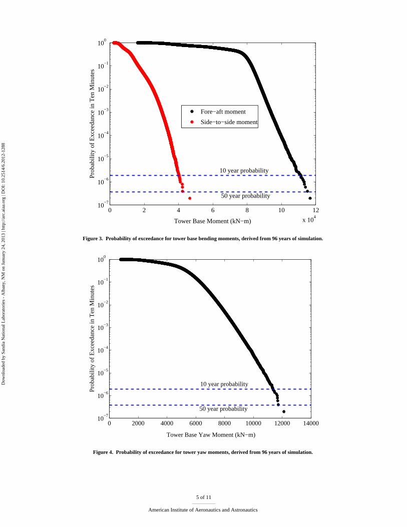
−7.Probability of exceedance plots for various wind turbine loads are shown in Figures 1 through 4. There is some

uncertainty in the extreme tails of the distributions, but,in general, the distributions are well-defined down to a prob-ability level of10

−6, corresponding approximately to a twenty year return load.The tails of the distributions are alsoall well-behaved, in the sense that there are no large changes in slope or other unexpected behavior beyond the “knee”in the distribution. This provides additional confidence inextrapolation approaches, where limited simulation data areused to extrapolate to long-term return loads. For example,suppose one week’s worth of simulations were performed(approximately 1000 simulations), such that the lowest probability of exceedance computed was approximately10

−3.Examining Figure 1, extrapolation of a distribution definedeven down to10

−2 would yield good estimates of a fiftyyear return period load. However, the tails of the distributions do follow different shapes, depending on the load. Forexample, Figure 3 shows that the tail of the tower base side-to-side moment is convex, whereas the tail of the towerfore-aft moment distribution is concave. The generated database should prove useful in assessing and calibratingdifferent load extrapolation strategies.

Presentation of maximum loads for each simulation as a function of mean wind speed is also illustrative; thisallows us to identify the mean wind speed or speeds for which load extremes occur. Figure 5 shows the maximumtip deflections versus mean wind speed. The largest out-of-plane deflections occur between the rated wind speed andapproximately 20 m/s, although there is one rather large deflection that occurs at around 22.5 m/s. The extreme in-plane tip deflections increase monotonically with wind speed. For both out-of-plane and in-plane tip deflections, thedistribution widens as the mean wind speed increases. Figure 6 shows similar distributions for flap-wise and edge-wiseblade root bending moments. The flap-wise moment distribution variation with mean wind speed is similar to that ofthe out-of-plane tip deflection. The edge-wise tip deflection extremes increase up to rated wind speed, then dip downas wind speed increases to 20 m/s, and finally increase again towards cut-out. The rather clean lower bounds on thesedistributions make physical sense: a baseline oscillationof blade flap moment is expected due to mean wind shear,while cyclical gravity loadings establish a baseline for the edgewise moment.

3 of 11

American Institute of Aeronautics and Astronautics

Dow

nloa

ded

by S

andi

a N

atio

nal L

abor

ator

ies

- A

lban

y, N

M o

n Ja

nuar

y 24

, 201

3 | h

ttp://

arc.

aiaa

.org

| D

OI:

10.

2514

/6.2

012-

1288

0 1 2 3 4 5 6 7 8 9 10 11 1210

−7

10−6

10−5

10−4

10−3

10−2

10−1

100

Blade Tip Deflection (m)

Pro

babi

lity

of E

xcee

danc

e in

Ten

Min

utes

10 year probability

50 year probability

Out−of−plane deflection

In−plane deflection

Figure 1. Probability of exceedance for blade tip deflections, derived from 96 years of simulation.

0 0.2 0.4 0.6 0.8 1 1.2 1.4 1.6 1.8 2

x 104

10−7

10−6

10−5

10−4

10−3

10−2

10−1

100

Blade Root Bending Moment (kN−m)

Pro

babi

lity

of E

xcee

danc

e in

Ten

Min

utes

10 year probability

50 year probability

Flapwise moment

Edgewise moment

Figure 2. Probability of exceedance for blade root bending moments, derived from 96 years of simulation.

4 of 11

American Institute of Aeronautics and Astronautics

Dow

nloa

ded

by S

andi

a N

atio

nal L

abor

ator

ies

- A

lban

y, N

M o

n Ja

nuar

y 24

, 201

3 | h

ttp://

arc.

aiaa

.org

| D

OI:

10.

2514

/6.2

012-

1288

0 2 4 6 8 10 12

x 104

10−7

10−6

10−5

10−4

10−3

10−2

10−1

100

Tower Base Moment (kN−m)

Pro

babi

lity

of E

xcee

danc

e in

Ten

Min

utes

10 year probability

50 year probability

Fore−aft moment

Side−to−side moment

Figure 3. Probability of exceedance for tower base bending moments, derived from 96 years of simulation.

0 2000 4000 6000 8000 10000 12000 1400010

−7

10−6

10−5

10−4

10−3

10−2

10−1

100

Tower Base Yaw Moment (kN−m)

Pro

babi

lity

of E

xcee

danc

e in

Ten

Min

utes

50 year probability

10 year probability

Figure 4. Probability of exceedance for tower yaw moments, derived from 96 years of simulation.

5 of 11

American Institute of Aeronautics and Astronautics

Dow

nloa

ded

by S

andi

a N

atio

nal L

abor

ator

ies

- A

lban

y, N

M o

n Ja

nuar

y 24

, 201

3 | h

ttp://

arc.

aiaa

.org

| D

OI:

10.

2514

/6.2

012-

1288

(a) Out-of-plane tip deflection. (b) In-plane tip deflection.

Figure 5. Maximum tip deflection versus mean wind speed, derived from 96 years of simulation.

(a) Flap-wise blade root bending moment. (b) Edge-wise blade root bending moment.

Figure 6. Maximum blade bending moments versus mean wind speed, derived from 96 years of simulation.

(a) Tower base fore-aft moment. (b) Tower base yaw moment.

Figure 7. Maximum tower moments versus mean wind speed, derived from 96 years of simulation.

6 of 11

American Institute of Aeronautics and Astronautics

Dow

nloa

ded

by S

andi

a N

atio

nal L

abor

ator

ies

- A

lban

y, N

M o

n Ja

nuar

y 24

, 201

3 | h

ttp://

arc.

aiaa

.org

| D

OI:

10.

2514

/6.2

012-

1288

The tower fore-aft and yaw moment extremes are plotted versus mean wind speed in Figure 7. The fore-aft momentdistribution is relatively narrow up to the rated wind speed, then widens substantially beyond 15 m/s with the largestextremes occurring between 15 and 22 m/s. The tower yaw moment increases more or less monotonicaly with meanwind speed, increasing less rapidly above the rated wind speed. The largest extremes occur between 15 and 20 m/salthough significant extremes occur near the cut-out wind speed as well.

V. Extreme Load Cases

The random seed and mean wind speed used to generate the turbulent wind field were saved for each simulation,allowing any particularly interesting simulations to be reproduced later and studied in detail, if desired. The largestextreme load cases were re-run for several loads of interestin order to gain insight into the relationship between theincident wind field and resulting extreme loads.

Figure 8 shows time histories for the simulation that led to the maximum out-of-plane blade tip deflection. Themean hub height wind speed for this simulation was 15.51 m/s.The wind speed decreases to almost 6 m/s, then rampsup to about 14 m/s over a period of about ten seconds. During this ramp up, the horizontal wind direction fluctuatesaround a value of approximately ten degrees. Meanwhile, prior to the ramp up in wind speed, the blade pitch anglehas reduced to its minimum value due to the initial decrease in wind speed. The blade pitch is unable to respondquickly enough to avoid the large extremum in tip deflection associated with the ramp-up in wind speed. Note thattime histories of hub-height wind speed and direction may only partially explain the causes of extreme loads. Thespatial structure of the turbulent wind field may also play animportant role and is worth examining in greater detailin the future. The details of how a wind field effectively excites wind turbine structural motions of interest are alsoimportant.

Figure 9 shows time histories for the simulation resulting in the maximum observed blade root flap moment. Themean wind speed for this case was 19.94 m/s. Similar to the maximum tip deflection case, the wind speed ramps downfrom above the rated wind speed to below the rated wind speed,then ramps up fairly rapidly ahead of the extremeloads, with the blade pitch system unable to respond quicklyenough. In this case, the vertical wind direction changessuddenly, increasing from about -10 degrees to +2 degrees within two seconds. The blade flap moment, which hadpreviously been oscillating at a once-per-rev frequency, jumps up to the extreme value simultaneously with the rampin vertical wind direction.

VI. Aerodynamic Model Uncertainty

As mentioned previously, the aero-elastic loads simulations were performed using the ‘equilibrium’ wake modelwithin AeroDyn, the program that provides aerodynamic loads to FAST. The equilibrium wake model, based on bladeelement momentum theory, assumes that the rotor wake responds immediately to the applied blade loads, such thatthe wake response, induced flow from the wake, and blade loadsalways remain in equilibrium. The other availablemodel within AeroDyn is the generalized dynamic wake (GDW) model.10 The GDW model solves a set of ordinarydifferential equations for the induced flow from the wake. This set of equations introduces a time lag between theblade loadings and the response of the wake, resulting in a more physically realistic description of the induced flow.

Simulations were initially run with the GDW model; however,a significant portion of these simulations resultedin unstable aero-elastic responses. The instabilities occurred within a range of mean wind speeds from 8 m/s to 10.5m/s. The GDW model within AeroDyn is hard-coded to switch to the equilibrium wake model below 8 m/s, due toknown problems with instabilities at low wind speeds.

As a second alternative, the ECN wake model11 was implemented within AeroDyn. This model, also based on asolution to an ordinary differential equation, is significantly simpler than the GDW model but accounts for wake timelag effects. The ECN model also produced instabilities, although considerably fewer runs went unstable for the ECNmodel than for the GDW model. Figure 10 compares the maximum tip deflection versus wind speed for the equilibriumand ECN wake models. Several unstable results using the ECN model that resulted in a high-amplitude, unphysicallimit cycle are visible, while several additional simulations went completely unstable and “blew up.” While the obviousunstable results may be filtered out from the data set, it becomes difficult to differentiate unphysical instabilities andreal, large-amplitude extreme events. For this reason, theequilibrium wake model was used to generate the loadsdatabase. Figure 10 indicates that the equilibrium model provides a conservative estimate of tip deflections relative toa dynamic wake model. Future work should focus on improvement of the stability of dynamic wake models to enabletheir use in the context of massive numbers of loads simulations.

7 of 11

American Institute of Aeronautics and Astronautics

Dow

nloa

ded

by S

andi

a N

atio

nal L

abor

ator

ies

- A

lban

y, N

M o

n Ja

nuar

y 24

, 201

3 | h

ttp://

arc.

aiaa

.org

| D

OI:

10.

2514

/6.2

012-

1288

VII. Summary

This paper has described the use of high-performance computing resources to simulate wind turbine loads overmultiple turbine lifetimes. This capability allows for direct estimation of extreme loads, generation of databases fordirect testing of load extrapolation techniques, and identification of important loading mechanisms present in stochasticwind fields. We anticipate that large-scale load simulations using high-performance computing can play an integralrole in developing future wind turbine design standards. A key challenge to the approach, identified in the presentstudy, is the robustness of dynamic wake aerodynamic modelsover a large range of inflow conditions. Dynamic wakeeffects have important impacts on wind turbine loads, and itis desirable to incorporate these effects into comprehensiveloads studies.

There are potentially many other ways that high-performance computing can impact the study of wind turbineloads. Other input parameters, such as turbulence intensity and mean wind shear, can be treated as uncertain or ran-dom, following assumed probability distributions. The simulations can also be used to characterize concurrent loads;for example, it is useful to define the probability of achieving a certain edge-wise blade bending moment when theflap-wise bending moment concurrently exceeds some threshold. Fatigue calculations using a massive loads databasewould allow for testing of assumptions made during a wind turbine fatigue analysis. Finally, high-performance com-puting resources are anticipated to be even more valuable when considering the more complicated case of an offshorewind turbine, where combined wind and wave loadings must be considered.

References1International Electrotechnical Commission. IEC 61400-1 Ed.3: Wind turbines - Part 1: Design requirements, 2005.2P. Moriarty. Database for validation of design load extrapolation techniques.Wind Energy, 11(6):559–576, 2008.3J. Jonkman, S. Butterfield, W. Musial, and G. Scott. Definitionof a 5-MW reference wind turbine for offshore system development. Technical

Report NREL/TP-500-38060, 2009.4D.J. Malcolm and A.C. Hansen. WindPACT turbine rotor designstudy. Technical Report NREL/TP-500-32495, 2006.5J.M. Jonkman and M.L. Buhl. FAST User’s Guide. NREL/EL-500-29798, 2005.6B.J. Jonkman and J.M. Jonkman. Documentation of updates to FAST, A2AD. and AeroDyn Released March 31,2010, including the revised

AeroDyn interface. Unpublished NREL Technical Report, 2010.7B.J. Jonkman. TurbSim user’s guide: Version 1.50. NREL/TP-500-46198, 2009.8B.M. Adams, W.J. Bohnhoff, K.R. Dalbey, J.P. Eddy, M.S. Eldred, D.M. Gay, K. Haskell, P.D. Hough, and L.P. Swiler. DAKOTA,a

multilevel parallel object-oriented framework for design optimization, parameter estimation, uncertainty quantification, and sensitivity analysis:Version 5.0 user’s manual. Sandia Technical Report SAND2010-2183, December 2009.

9M.D. McKay, R.J. Beckman, and W.J. Conover. A comparison of three methods for selecting values of input variables in the analysis ofoutput from a computer code.Technometrics, 21(2):239–245, 1979.

10A. Suzuki.Application of dynamic inflow theory to wind turbine rotors. PhD thesis, The University of Utah, August 2000.11H. Snel. Survey of induction dynamics modelling within BEM-like codes: Dynamic inflow and yawed flow modelling revisi ted. AIAA

Paper 2001-0027, 2001.

8 of 11

American Institute of Aeronautics and Astronautics

Dow

nloa

ded

by S

andi

a N

atio

nal L

abor

ator

ies

- A

lban

y, N

M o

n Ja

nuar

y 24

, 201

3 | h

ttp://

arc.

aiaa

.org

| D

OI:

10.

2514

/6.2

012-

1288

580 590 600 610 620 630 6405

10

15

20

Hub

ht.

win

d sp

d. (

m/s

)

580 590 600 610 620 630 640

−10

0

10

20

Hor

iz. w

ind

dir.

(de

g)

580 590 600 610 620 630 640

0

10

20

Bla

de p

itch

(deg

.)

580 590 600 610 620 630 6400

5

10

Bla

de 2

tip

defl.

(m

)

Time (sec)

Figure 8. Time history of hub height longitudinal wind speed, hub height wind direction in the horizontal plane, and blade 2 out-of-planetip deflection. Simulation 403,729 (maximum out-of-plane tip deflection).

9 of 11

American Institute of Aeronautics and Astronautics

Dow

nloa

ded

by S

andi

a N

atio

nal L

abor

ator

ies

- A

lban

y, N

M o

n Ja

nuar

y 24

, 201

3 | h

ttp://

arc.

aiaa

.org

| D

OI:

10.

2514

/6.2

012-

1288

340 350 360 370 380 390 400

10

20

30

Hub

ht.

win

d sp

d. (

m/s

)

340 350 360 370 380 390 400−10

0

10

Ver

t. w

ind

dir.

(de

g)

340 350 360 370 380 390 400

0

10

20

Bla

de p

itch

(deg

.)

340 350 360 370 380 390 400

0

10000

20000

Bla

de 3

Fla

p M

om. (

kN−

m)

Time (sec)

Figure 9. Time history of hub height longitudinal wind speed, hub height wind direction in the vertical plane, blade pitch angle, and blade3 root flap moment. Simulation 1,662,822 (maximum blade rootflap moment).

10 of 11

American Institute of Aeronautics and Astronautics

Dow

nloa

ded

by S

andi

a N

atio

nal L

abor

ator

ies

- A

lban

y, N

M o

n Ja

nuar

y 24

, 201

3 | h

ttp://

arc.

aiaa

.org

| D

OI:

10.

2514

/6.2

012-

1288

Figure 10. Comparison of extreme values for out-of-plane blade tip deflection predicted by the equilibrium and ECN wake models, derivedfrom 16 years of simulation.

11 of 11

American Institute of Aeronautics and Astronautics

Dow

nloa

ded

by S

andi

a N

atio

nal L

abor

ator

ies

- A

lban

y, N

M o

n Ja

nuar

y 24

, 201

3 | h

ttp://

arc.

aiaa

.org

| D

OI:

10.

2514

/6.2

012-

1288