Expected wind turbine load estimation based on the wind field joint pdf

constructed using the mixture Gaussian-EM algorithm.

Jinkyoo Park

December 14, 2012

1 Introduction

1.1 Motivation

The stable boundary layer (SBL) is a stably stratified atmo-spheric layer that usually forms in the night over land whenthe earth cools as a result of a net loss of radiation[7]. Thewind field characteristics in SBL distinctly differ from thosein unstable boundary layer that forms in the daytime. Fig-ures 1(a) and 1(b) show how the longitudinal wind speedand the wind direction change with the time. The vari-ations in wind field characteristics accordingly affect thewind turbine responses such as extreme load, power out-put, and fatigue damage. Understandings in the wind fieldcharacteristics variation and the corresponding impacts ona wind turbine, therefore, very important not only for de-signing but also for managing a wind turbine effectively.

(a) Longitudinal wind speed (b) Wind direction

Figure 1: Evolution of the wind field with time. The 3Dwind field is simulated by large-eddy simulation by ProfBasu from NCSU

1.2 Objective

The machine learning algorithms are applied, in this paper,to understand i) how the wind field characteristics changedepending on atmospheric conditions and ii) how wind tur-bine loads are affected by different wind field characteris-tics. The variations in wind field characteristics are investi-gated by comparing the joint probability distribution func-tion (PDF) for wind field input features. Gaussian MixtureModel (GMM) is implemented to construct the PDFs con-ditional on the time, day and night times. The influence ofwind field on wind turbine loads are studied by constructingthe wind turbine load classification model mapping windfield input features to wind turbine load statistics. To this

end, multi-class classification algorithm based on GaussianDiscriminative Analysis (GDA) is implemented.

On the basis of the two separately constructed statisticalmodels, the joint pdf for wind field features and the windturbine load classification function, the expected wind tur-bine class can be calculated in a probability framework.From a lifetime health monitoring perspective, it is impor-tant to tack the expected wind turbine load given a cer-tain atmospheric condition rather than simply identifyingabnormal loads. The instantaneously monitored abnormalloads do not necessarily indicate the deterioration in a windturbine system since these loads can be caused by strongwind in a short duration. In contrast, if the expected loadchanges over a time, it can possibly indicate that the sys-tem is under abnormal conditions. The expected wind tur-bine load classes are compared between the day and nighttime conditions as an example. The overall framework andobjectives are summarized in Figure 2.

Figure 2: Machine learning approaches and the objectives

2 Methodology

2.1 Input and output data

We use wind fields simulated by the computational fluid dy-namic code (large eddy simulation) and the correspondingwind turbine load responses simulated by the aerodynamicwind turbine load analysis code (FAST[3]). The charac-teristics of a 10-min long wind field are described by time-averaged statistics. The mean wind speed at a wind turbinehub height µU , the power exponent α describing the steep-ness of the vertical wind profile, and the standard deviation

1

of wind speed σU measuring the level of turbulence. Windturbine blade bending moment statistics, the 10-min max-imum load and the equivalent fatigue damage, are used asoutputs. The input and output statistics are depicted inFigure 3

Figure 3: Wind field input features and the output loadstatistics

2.2 Procedures

Figure 4: Implementation of machine learning algorithmson the extracted data set

To validate the proposed framework, we compare theexpected wind turbine loads between the two operatingtimes, day (unstable atmosphere) and night (stable atmo-sphere). Given 2,200 10-min wind field time series andthe corresponding 2,200 wind turbine load times series,we extract the 2200 sets of input wind feature vectors,x = (µU , α, σU ), and the corresponding 2200 load statis-tics y = (yMax, yEFL). Figure 4 shows how the sets ofwind field input feature vectors and the wind turbine loadstatistics are used for modeling the statistical model viathe GMM and the GDA. For the GMM, we first classifywind field input data into two groups, day time and nighttime data on the basis of the time. Then, the conditionalPDFs are modeled for the day time fX|W (x(i)|w = day)

and for the night time fX|W (x(i)|w = night) using GMM

and EM algorithm. The two PDFs can be updated duringthe daytime and the night time, respectively. With respectto GDA, the wind field input data are divided into train-ing and testing data sets, both of which consists of 1100sets of input output pairs (x(i), y(i)). The wind input fea-tures from both daytime and the night time are includedto the training data to exposure the the leaning algorithmto wide range of input feature space. Note that the GDAalgorithm can be continuously updated regardlessly of thetime since the output are assumed to depend only on theinput feature vector x

3 Background

3.1 Gaussian discriminative analysis

There are two types of classification methods in machinelearning. One is discriminativeapproach that directly mapinput x to output y using parametric fitting. The otherapproach is generativealgorithm differentiating data on thebasis of input features’ distributional information learnedfrom data. For both classification methods, two-class,binary classification algorithm have been matured, whilemulti-class classification has not yet extensively studied. [1]surveyed different type of supervised multi-class classifica-tion methods, most of which are based on binary classifica-tions. [4] has proposed Linear Discriminative in classifyingmulti labeling problem. In this study, Gaussian Discrimi-native Analysis (GDA) will be implemented in classifyingthe wind turbine load statistics.

The wind turbine load function l(x) is constructed usingthe Gaussian Discriminative Analysis (GDA). The GDAis a generative learning algorithm that classify the inputfeature’s label using the learned input feature distribution.Given the training data set, the posterior distribution on ygiven x is modeled according to Bayes rule as follows:

p(y|x) = p(x|y)p(y)p(x)

=p(x|y)p(y)

Σyp(x|y)p(y)(1)

where p(x|y) is the input feature distribution given the out-put label y, and p(y) is the class priori. Then, to classifythe label for the new input feature xnew , the label can beselected according to the maximum a posteriori detection(MAP) principle as follows:

y = argmaxy

P (y|xnew) = argmaxy

p(xnew |y)p(y)P (xnew)

= argmaxy

p(xnew |y)p(y)(2)

In particular, GDA models p(x|y = j) using the multivari-ate normal distribution as follows:

p(x|y = j) =1

√

(2π)n|Σ|exp

(

− (x− µj)TΣ−1(x− µj)

2

)

(3)and the class prior is modeled as:

p(y = j) = φj ∼ Multinormial(φ) (4)

2

The parameters φ, Σ, and µ can be found based on themaximum likelihood (ML) estimation. The log-likelihoodof the data is given by

l(φ, µ,Σ) = log

m∏

i=1

p(x(i), y(i);φ, µ,Σ)

= log

m∏

i=1

p(x(i)|y(i);µ,Σ)p(y(i);φ)(5)

and the parameters can be found By maximizing Eqn 5with respect, respectively, to µ,Σ, and φ, the parameterscan be obtained.

3.2 Mixtures of Gaussian Model Density

Estimation Using EM

Finite mixture models are effective way for statistical mod-eling of data, which has been widely used for unsupervisedclustering and density estimation[2]. In structural healthmonitoring community, Gaussian mixture model has beenused for identifying damages in a structure on the basisof estimated output feature distribution[5]. In this paper,the wind field features characterizing the wind field are de-picted by the their joint probabiilty density function con-structed by Gaussian mixture model. The centers, shapes,and dispersion of PDFs depending on different atmosphericcondition can give us insight into how the wind field evolves.

The join PDF fX|W (x|w) conditional on an atmosphericcondition w is constructed on the basis of the Mixturesof Gaussian model whose parameters are derived by theExpectation Maximization (EM) algorithm. The mixturedensity is given as

f(x) =k∑

j=1

φjfj(x) =k∑

j=1

φjp(x|µj , σj) (6)

where p(x|µk, σk) is the density of kth component, and it isexpressed, in Gaussian Mixture Model (GMM), as a jointPDF for x as

p(x|µj , σj) =1

√

(2π)n|Σj |exp

(

−(x− µj)

TΣ−1j (x− µj)

2

)

(7)In addition, φk is the weight (probability) of the jth Gaus-sian component.

To construct the mixture density we need to estimate theparameters µk, σk, and φk for each kth component. Giventhe independent data sets {x(1), ..., x(m)}, the log-likelihoodof the data is represented as

l(θ) =m∑

i=1

log p(x(i);φ, µ,Σ)

=

m∑

i=1

log

k∑

z(i)=1

p(x(i)|z(i);µ,Σ)p(z(i);φ)(8)

where z(i) is the random variable drawn from the kth pos-sible values (z(i) ∼ Multinomial(φ)), and it specifies one

of the k possible Gaussian components from which x(i) isdrawn. When z(i) = j, p(x(i), z(i);µ,Σ) ∼ N(µj , σj) andp(z(i) = j|φ) = φj . The fact that z(i) is not known makesthe estimation of parameters based on the maximum like-lihood principle difficult.

The expectation-maximization (EM) algorithm gives anefficient method for estimating parameters given the hidden(latent) random variables. The EM algorithm is composedof the two iterative steps: i) E-steps - evaluate the prob-ability of z(i) given the current data and the previouslyestimated parameters as follows:

Qi(z(i) = p(z(i)|x(i);µ,Σ, φ) (9)

and ii) E-step - choose the parameters that maximize thelikelihood function

m∑

i=1

k∑

z(i)=1

Qi(z(i))log

p(x(i), z(i);µ,Σ)p(z(i);φ)

Qi(z(i))

=

m∑

i=1

k∑

j=1

Qi(z(i) = j)log

p(x(i)|z(i) = j;µ,Σ)p(z(i) = j;φ)

Qi(z(i) = j)

=

m∑

i=1

k∑

j=1

wij log

1√(2π)n|Σk|

exp

(

− (x−µj)TΣ−1

j(x−µj)

2

)

φj

wij

(10)where wi

j = Qi(z(i) = j) is the soft classifier representing

the probability that x(i) is drawn from the jth Gaussiancomponent. In general EM framework, E-step is equivalentto constructing the lower bound on the likelihood function,and M-step is equivalent to maximizing the lower boundedmaximum likelihood function. These two steps continueuntil the parameters converge. The formulas are from [6]

3.3 Expected Wind Turbine Load Class

The expected wind turbine load can be described as

E[y|w] =∫

x

y(x)fX|W (x|w)dx (11)

where y is the wind turbine load, x is the wind field char-acteristic feature vector, and w represents the external at-mospheric condition (e.g., location, time). To evaluate theexpected load, the two functions are need to be defined:y(x) mapping the input wind field features to the corre-sponding wind turbine load and fX|W (x|w) describing thejoint PDF for wind field input features given a certain at-mospheric condition. Note that the wind turbine loads onlydepend on the wind field input features x, and the PDF forx is subject to change according to different atmosphericconditions. In this sense, E[y|w] can give us deep insightsinto how a wind turbine experiences different levels of aload given a easily observable atmospheric condition. Inaddition, the variation of E[y|w] can possibly indicate thedeterioration in a structure.

3

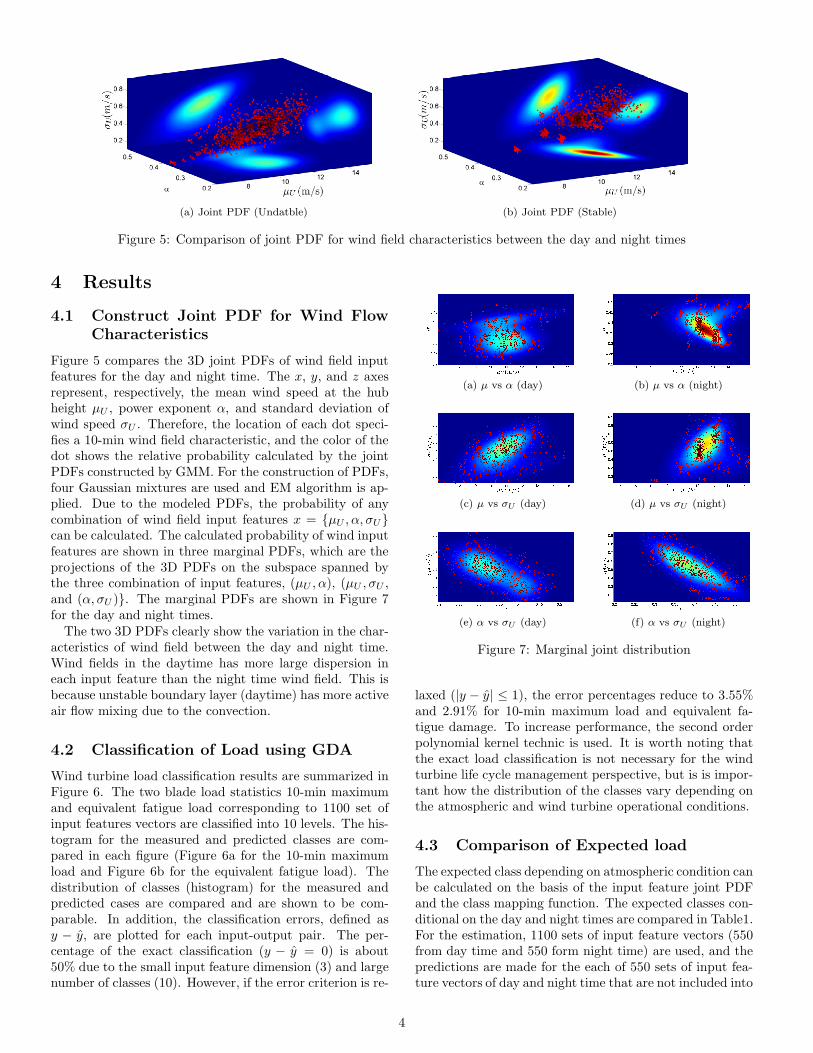
(a) Joint PDF (Undatble) (b) Joint PDF (Stable)

Figure 5: Comparison of joint PDF for wind field characteristics between the day and night times

4 Results

4.1 Construct Joint PDF for Wind Flow

Characteristics

Figure 5 compares the 3D joint PDFs of wind field inputfeatures for the day and night time. The x, y, and z axesrepresent, respectively, the mean wind speed at the hubheight µU , power exponent α, and standard deviation ofwind speed σU . Therefore, the location of each dot speci-fies a 10-min wind field characteristic, and the color of thedot shows the relative probability calculated by the jointPDFs constructed by GMM. For the construction of PDFs,four Gaussian mixtures are used and EM algorithm is ap-plied. Due to the modeled PDFs, the probability of anycombination of wind field input features x = {µU , α, σU}can be calculated. The calculated probability of wind inputfeatures are shown in three marginal PDFs, which are theprojections of the 3D PDFs on the subspace spanned bythe three combination of input features, (µU , α), (µU , σU ,and (α, σU )}. The marginal PDFs are shown in Figure 7for the day and night times.The two 3D PDFs clearly show the variation in the char-

acteristics of wind field between the day and night time.Wind fields in the daytime has more large dispersion ineach input feature than the night time wind field. This isbecause unstable boundary layer (daytime) has more activeair flow mixing due to the convection.

4.2 Classification of Load using GDA

Wind turbine load classification results are summarized inFigure 6. The two blade load statistics 10-min maximumand equivalent fatigue load corresponding to 1100 set ofinput features vectors are classified into 10 levels. The his-togram for the measured and predicted classes are com-pared in each figure (Figure 6a for the 10-min maximumload and Figure 6b for the equivalent fatigue load). Thedistribution of classes (histogram) for the measured andpredicted cases are compared and are shown to be com-parable. In addition, the classification errors, defined asy − y, are plotted for each input-output pair. The per-centage of the exact classification (y − y = 0) is about50% due to the small input feature dimension (3) and largenumber of classes (10). However, if the error criterion is re-

(a) µ vs α (day) (b) µ vs α (night)

(c) µ vs σU (day) (d) µ vs σU (night)

(e) α vs σU (day) (f) α vs σU (night)

Figure 7: Marginal joint distribution

laxed (|y − y| ≤ 1), the error percentages reduce to 3.55%and 2.91% for 10-min maximum load and equivalent fa-tigue damage. To increase performance, the second orderpolynomial kernel technic is used. It is worth noting thatthe exact load classification is not necessary for the windturbine life cycle management perspective, but is is impor-tant how the distribution of the classes vary depending onthe atmospheric and wind turbine operational conditions.

4.3 Comparison of Expected load

The expected class depending on atmospheric condition canbe calculated on the basis of the input feature joint PDFand the class mapping function. The expected classes con-ditional on the day and night times are compared in Table1.For the estimation, 1100 sets of input feature vectors (550from day time and 550 form night time) are used, and thepredictions are made for the each of 550 sets of input fea-ture vectors of day and night time that are not included into

4

2 4 6 8 100

200

400

class yMax

Fre

quen

cy

Measured class

2 4 6 8 100

200

400

class yMax

Fre

quen

cy

Prediction

0 200 400 600 800 1000−5

0

5

data i

y−

y Error bound

(a) Maximum load

2 4 6 8 100

200

400

class yEFL

Fre

quen

cy

Measured class

2 4 6 8 100

200

400

class yEFL

Fre

quen

cy

Prediction

0 200 400 600 800 1000−5

0

5

data i

y−

y Error bound

(b) EFL

Figure 6: Multi labels Gaussian discriminative analysis: comparison between measured and predicted classes. |y − y| ≥ 1is considered as error. The error rate for yMax is 3.55 % and the error rate for yEFL is 2.91 %

Table 1: Comparison of the expected classes conditional onthe wind turbine operational time

Measured classes Predicted classes∑

Nwi=1 y

(i)fX|W (x(i)|w)∑

Nwi=1 y(x

(i))fX|W (x(i)|w)

w=day w=night w=day w=night

E(ymax (MN-m) 7.9379 8.3024 7.9320 8.4337

E(yEFL (MN-m) 5.4452 7.4850 5.3040 7.5471

the training data. The effectiveness of statistical model canbe evaluated by comparing the expected class based on themeasured class and the predicted class, which show a greatagreements. The trend of load statistic variations can bestudied by comparing the day and night time expected val-ues. Both of the expected load classes, especially EFL, arehigher in the night time, whose trends are well captured bythe statistical model used in this research.

5 Conclusion

In terms of the Statistical models,

• Gaussian Mixture model can be used for constructinga joint PDF for wind field input characteristics

• Gaussian Discriminative analysis can effectively pre-dict the wind turbine blade load classes, even for mul-tiple classes.

• GDA and GMM model can be integrated to estimatethe expected wind turbine load in a certain condition.

For the understanding of wind field and wind turbineload output characteristics,

• In the night, wind speed is faster, less turbulent, andincrease sharply with height. In addition, turbulenceand the shear profile is negatively correlated.

• Maximum wind turbine blade load is higher in the daytime, but the fatigue load higher in the night time.

6 Acknowledgement

The author would like to acknowledge the advice from Prof.Law, Stanford (CEE), and wind field input data providedby Prof. Basu, NCSU.

References

[1] Mohamed Aly. Survey on multiclass classification meth-ods, 2005.

[2] Mario A.T. Figueiredo and Anil K. Jain. Unsupervisedlearning of finite mixture models. IEEE transactions of

pattern analysis and machine intelligence, 24, 2002.

[3] J. M. Jonkman and M. L. Buhl. FAST User’s Guide.Technical Report NREL/EL-500-38230, National Re-newable Energy Laboratory, Golden, Co, 2005.

[4] Tao. Li, Shenghuo. Zhu, and Mitsounori Ogihara. Usingdiscriminative analysis for multi-class classification: anexperimental investigation. Journal of Konwledge and

Information Systems, 10:453–472, 2006.

[5] K. Krishnan Nair and Anne S. Kiremidjian. Time se-ries based structural damage detection algorithm usinggaussian mixture modeling. Journal of Dynamic sys-

tems, Measurement, and Control, 129:285–293, 2007.

[6] Andrew Ng. The EM algorithm. Stanford University,CS229 Machine Learning Lecture note.

[7] R. B. Stull. An Introduction to Boundary Layer Mete-

orology. Kluwer Academic Publishers, 1988.

5