Georgia State University Georgia State University

ScholarWorks @ Georgia State University ScholarWorks @ Georgia State University

Computer Science Theses Department of Computer Science

12-4-2006

DCT Implementation on GPU DCT Implementation on GPU

Serpil Tokdemir

Follow this and additional works at: https://scholarworks.gsu.edu/cs_theses

Part of the Computer Sciences Commons

Recommended Citation Recommended Citation Tokdemir, Serpil, "DCT Implementation on GPU." Thesis, Georgia State University, 2006. https://scholarworks.gsu.edu/cs_theses/33

This Thesis is brought to you for free and open access by the Department of Computer Science at ScholarWorks @ Georgia State University. It has been accepted for inclusion in Computer Science Theses by an authorized administrator of ScholarWorks @ Georgia State University. For more information, please contact scholarworks@gsu.edu.

DIGITAL COMPRESSION ON GPU

by

SERPIL TOKDEMIR

Under the Direction of Saeid Belkasim

ABSTRACT

There has been a great progress in the field of graphics processors. Since, there is no rise in the

speed of the normal CPU processors; Designers are coming up with multi-core, parallel

processors. Because of their popularity in parallel processing, GPUs are becoming more and more

attractive for many applications. With the increasing demand in utilizing GPUs, there is a great

need to develop operating systems that handle the GPU to full capacity. GPUs offer a very

efficient environment for many image processing applications. This thesis explores the processing

power of GPUs for digital image compression using discrete cosine transform.

INDEX WORDS: Digital Image Compression, DCT/IDCT, Cg, GPU

DIGITAL COMPRESSION ON GPU

by

SERPIL TOKDEMIR

A Thesis Submitted in Partial Fulfillment of the Requirements for the Degree of

Master of Science

In the College of Arts and Sciences

Georgia State University

2006

Copyright by

Serpil Tokdemir

2006

DIGITAL COMPRESSION ON GPU

by

SERPIL TOKDEMIR

Major Professor: Saeid Belkasim Committee: A. P. Preethy Ying Zhu

Electronic Version Approved:

Office of Graduate Studies

College of Arts and Sciences

Georgia State University

December,2006

iv

ACKNOWLEDGEMENTS

I would like to express my gratitude to my supervisor, Dr. Saeid Belkasim, whose

expertise, understanding, and patience, added considerably to my graduate experience. I

appreciate his vast knowledge and skill in many areas. This thesis would not appear in its present

form without the kind assistance and support of him.

I would like to thank the other members of my committee, Dr. Ying Zhu, who guided me in

new technologies and headed me go for my thesis topic, and Dr. A. P. Preethy, who was always

kind and willing to answer my questions, for the assistance they provided at all levels of the

research project.

A very special thanks goes out to Dr. Sibel Tokdemir, my sister, without whose motivation

and encouragement I would not have considered a graduate career in Computer Science.

I must also acknowledge Dr. Raj Sunderraman, without his support and good nature I

would never have been able to pursue Computer Science as a career.

I would also like to thank my family for the support they provided me through my entire

life and I must acknowledge my good friend, Milan Pandya, without whose encouragement and

assistance, I would not have finished this thesis.

Finally, I am grateful to Dr. Williams Nelson, who had faith on me and supported me

without any doubt by giving tuition waiving during my first calendar year in my degree.

v

TABLE OF CONTENTS ACKNOWLEDGEMENTS............................................................................................... iv LIST OF TABLES............................................................................................................ vii LIST OF FIGURES ......................................................................................................... viii LIST OF CHARTS ............................................................................................................ ix CHAPTER 1: INTRODUCTION....................................................................................... 1 CHAPTER 2: BASICS OF DIGITAL COMPRESSION................................................... 5

2.1. Why Do We Need Compression? ............................................................................ 5 2.2. What Are The Principles Behind Compression? ..................................................... 6 2.3. Image Compression Models .................................................................................... 8 2.4. Error-Free Compression......................................................................................... 10

2.4.1. Huffman Coding ............................................................................................. 11 2.4.2. Arithmetic Coding .......................................................................................... 12 2.4.3. LZW Coding ................................................................................................... 12 2.4.4. Bit Plane Coding ............................................................................................. 13 2.4.5. Lossless Predictive Coding ............................................................................. 13

2.5. Lossy compression................................................................................................. 14 2.5.1. What Does a Typical Image Coder Look Like in Lossy Compression?......... 14 2.5.2. Transform Coding........................................................................................... 15 2.5.3. Wavelet Coding .............................................................................................. 16 Similarities and Dissimilarities of Wavelet Coding and Transfer Coding ............... 20

2.6. Image Compression Standards............................................................................... 21 2.6.1. Binary Image Compression Standards............................................................ 21 2.6.2. Continuous Tone Still Image Compression Standards ................................... 22 2.6.3. Video Compression Standards........................................................................ 23

CHAPTER 3: INTRODUCTION TO GPU...................................................................... 24 3.1. Why GPGPU?........................................................................................................ 24 3.2. Overview of Programmable Graphics Hardware................................................... 25

3.2.1 Overview of the Graphics Pipeline .................................................................. 25 3.2.2 Programmable Hardware ................................................................................. 27 3.2.3. Introduction to the GPU Programming Model ............................................... 28 3.2.4. GPU Program Flow Control ........................................................................... 30

3.3. Programming Systems ........................................................................................... 31 3.4. GPGPU Techniques ............................................................................................... 34

3.4.1. Data Structures................................................................................................ 36 3.5. GPGPU Applications ............................................................................................. 38

3.5.1. Physically-Based Simulation .......................................................................... 38 3.5.2. Signal and Image Processing .......................................................................... 39

CHAPTER 4: FAST COMPRESSION TECHNIQUES .................................................. 40 4.1. JPEG: DCT-Based Image Coding Standard .......................................................... 40 4.2. Image Compression Based on Vector Quantization .............................................. 46

4.2.1. Fast Transformed Vector Quantization (FTVO)............................................. 47 4.3. Fractal Image Compression ................................................................................... 49

CHAPTER 5: IMPLEMENTATION OF DCT ON GPU................................................. 54 5.1. Approach................................................................................................................ 54

vi

5.2. Technique............................................................................................................... 54 CHAPTER 6: RESULTS.................................................................................................. 59

6.1. Test Images ............................................................................................................ 61 CHAPTER 7: CONCLUSION ......................................................................................... 67 Reference: ......................................................................................................................... 68 APPENDIX....................................................................................................................... 72 APPENDIX A................................................................................................................... 72 APPENDIX B ................................................................................................................... 74 APPENDIX C ................................................................................................................... 78

vii

LIST OF TABLES

Table 2.1: Multimedia Data Items and Required Size and Transmission Time ................. 6 Table 6.1 Time consuming of the GPU and CPU usage over the whole program ........... 66

viii

LIST OF FIGURES

Figure 2.1 General Compression System Model ................................................................ 8 Figure 2.2 Huffman Coding.............................................................................................. 12 Figure 2.3 Lossless Predictive Coding Model: encoder, decoder..................................... 13 Figure 2.4 A Typical Lossy Signal/Image Encoder.......................................................... 14 Figure 2.5 Lossy Predictive Coding Model: encoder and decoder................................... 15 Figure 2.6 A Transform Coding System: encoder and decoder........................................ 16 Figure 2.7 A Typical Wavelet Coding System: encoder and decoder............................. 18 Figure 2.9 Wavelet Transform of the Image “Lena” ........................................................ 18 Figure 2.8 (Left) Quantizer as a function whose output values are discrete. (Right) because the output values are discrete, a quantizer can be more simply represented only on one axis. ....................................................................................................................... 20 Figure 3.1 The modern graphics hardware pipeline. The vertex and fragment processor stages are both programmable by the user. ....................................................................... 26 Figure 4.1 JPEG Encoder Block Diagram ........................................................................ 43 Figure 4.2 JPEG Decoder Block Diagram........................................................................ 43 Figure 4.3 Zig-zag Sequence ............................................................................................ 45 Figure 4.4 Pepper – original image Figure 4.5 DCT of Peppers .................................. 46 Figure 4.6 Quality 20 - 91% Zeros Figure 4.7 Quality 10 – 94% Zeros ...................... 46 Figure 4.8 Image partitioned into blocks .......................................................................... 47 Figure 4.9 Quantization .................................................................................................... 48 Figure 4.10 Spiral Architecture with spiral addressing .................................................... 51 Figure 4.11 Testing Images: Building and boat................................................................ 52 Figure 4.12 Original and compressed ‘building’ in SA.................................................... 52 Figure 4.13 Original and compressed ‘boat’ in SA .......................................................... 52 Figure 5.1 2-D DCT.......................................................................................................... 54 Figure 5.2.1 signal flow graph for fast (scaled) 8-DCT according to Arai, Agui, Nakajima........................................................................................................................................... 56 Figure 5.2.2 signal flow graph for fast (scaled) 8-DCT according to Arai, Agui, Nakajima........................................................................................................................................... 56 Figure 5.3 Partitioning the odd and even parts of DCT.................................................... 57 Figure 5.4 Program View.................................................................................................. 60 Figure 5.5 Demo Output of the Compression Program .................................................... 61 Figure 5.14 eye.png Figure 5.15 After IDCT .............................................................. 62 Figure 5.14 Comic.png Figure 5.15 After IDCT ........................................................ 62 Figure 5.14 Child.png Figure 5.15 After IDCT.......................................................... 62 Figure 5.13 Original Image – serpil2.png......................................................................... 63 Figure 5.14 After DCT Figure 5.15 After IDCT ........................................................ 64 Figure 5.16 Original Image – serpil3.png......................................................................... 64 Figure 5.17 After DCT Figure 5.18 After IDCT ........................................................ 65

ix

LIST OF CHARTS

Chart 6.1 Proportional Time consumed according to size of an image ............................ 66

CHAPTER 1: INTRODUCTION

The rapid growth of digital imaging applications, including desktop publishing,

multimedia, teleconferencing, and high-definition television has increased the need for effective

and standardized image compression techniques [29]. At the present state of technology, the only

solution is to compress multimedia data before its storage and transmission, and decompress it at

the receiver for play back. Image compression addresses the problem of reducing the amount of

data required to present a digital image with acceptable image quality. The underlying basis of the

reduction process is the removal of redundant data. If the process of redundancy removing is

reversible, i.e. the exact reconstruction of the original image can be achieved, it is called lossless

image compression; otherwise, it is called lossy image compression. Lossless compression is an

error-free compression, but can only provide a compression ratio ranging between 2 to 10 [31].

On the other hand lossy image compression (irreversible compression) is based on compromising

the accuracy of the recovered image in exchange for more compression. Scientific or legal

considerations make lossy compression unacceptable for many high performance applications

such as geophysics, telemetry, non-destructive evaluation, and medical imaging, which will still

require lossless image compression [33]. Lossless compression is necessary for many high

performance applications such as geophysics, telemetry, nondestructive evaluation, and medical

imaging, which require exact recoveries of original images.

For still image compression, the ‘Joint Photographic Experts Group’ or JPEG standard has

been established by ISO (International Standards Organization) and IEC (International Electro-

Technical Commission). JPEG established the first international standard for still image

compression where the encoders and decoders are DCT-based. The JPEG standard specifies three

modes namely sequential, progressive, and hierarchical for lossy encoding, and one mode of

lossless encoding.

2

Fractal image compression is a relatively recent image compression method which exploits

similarities in different parts of the image. During more than two decades of development, the

Iterated Function System (IFS) based compression algorithm stands out as the most promising

direction for further research and improvement [30]. Another technique that is widely used is

Vector Quantization. Vector quantization (VQ) is a relatively efficient coding technique used in

digital image compression area. The image is partitioned into many blocks, and each block is

considered as a vector. It provides many attractive features for image coding applications with

high compression ratios [26]. One important feature of VQ is the possibility of achieving high

compression ratios with relatively small block sizes. Another important advantage of VQ image

compression is its fast decompression by table lookup technique.

Since many image processing techniques have sections which consist of a common

computation over many pixels, this fact makes image processing in general a prime topic for

acceleration on the GPU [14]. Digital image processing (DIP) appears to be especially well-

suited to current GPU hardware and APIs, due to the graphical nature of the GPU's processing

power. The GPU is especially well-suited to performing 2D convolutions and filters, as well as

morphological operations. Furthermore, programming the GPU version of these algorithms is a

straightforward process, allowing the developer to access pixel neighborhoods using a relative

indexing paradigm rather than a complicated modular arithmetic scheme for referencing 2D array

elements in main memory [6]. A GPU is no longer a fixed pipeline but is now better described as

a SIMD parallel processor or a streaming processor [16].

The evolution of consumer graphics cards in recent years has introduced the GPU as a

flexible vector-processor capable of coloring, shading, etc. in parallel. In the most recent

generations of Graphics Processing Units (GPUs), the capacities of per-pixel and texturing

operations have greatly increased. Digital image processing algorithms should be a good fit for

modern GPU hardware. Any digital image processing technique entails a repetitive operation on

3

the pixels of an image. Graphics processors are designed to perform a block of operations on

groups of vertices or pixels, and they do this very efficiently.

The Fourier transform is a well known and widely used tool in many image processing

techniques, including filtering, manipulation, correction, and compression [16]. Implementing the

FFT on the graphics card is relatively straightforward. Fourier domain processing is not currently

done for real-time graphics synthesis because performing transforms on a CPU requires data to be

moved to and from the graphics card, a serious bottleneck. However, the current generation of

graphics cards has the power, programmability, and floating point precision required to perform

the FFT efficiently.

Fractal compression allows fast decompression but has long encoding times. The most time

consuming part is the domain blocks searching from each range [11]. Ugo Erra presented a novel

approach to perform fractal image compression on programmable graphics hardware, which is the

first application that uses the GPU for image compression. Using programmable capabilities of

the GPUs, the large amount of inherent parallelism and memory bandwidth are exploited to

perform fast pairing search between portions of the image.

Bo Fang, Guobin Shen, Shipeng Li, and Huifang Chen proposed several techniques that are

presented for efficient implementation of DCT/IDCT on GPU which are using matrix

multiplication [5]. The computation on GPU is achieved through one or multiple rendering

passes. Among the proposed techniques, multiple channel technique makes the most contribution

towards the final performance. It alone doubles the speed. This reveals that GPU is indeed good

at parallel processing.

The thesis continues as follows: Chapter 2 discusses basics of the digital compression. Next

chapter, Chapter 3, gives a brief introduction about graphics processing unit (GPU). Chapter 4,

presents the proposed fast compression techniques till now and Chapter 5 represents the

approach, and implementing of DCT on GPU and a brief introduction to Cg programming

4

language. Chapter 6 represents experimental results. Chapter 7 represents the discussion and

contributions.

5

CHAPTER 2: BASICS OF DIGITAL COMPRESSION

Every day, an enormous amount of information is stored, processed, and transmitted

digitally. Since much of this on-line information is graphical or pictorial in nature, the storage and

communications requirements are immense. Uncompressed multimedia data requires

considerable storage capacity and transmission bandwidth. Despite rapid progress in mass-storage

density, processor speeds, and digital communication system performance, demand for data

storage capacity and data-transmission bandwidth continues to outstrip the capabilities of

available technologies. The recent growth of data intensive multimedia-based web applications

have not only sustained the need for more efficient ways to encode signals and images but have

made compression of such signals central to storage and communication technology.

2.1. Why Do We Need Compression?

Image compression addresses the problem of reducing the amount of data required to

present a digital image with acceptable image quality. The underlying basis of the reduction

process is the removal of redundant data [32]. Interest in image compression dates back more

than 35 years. The initial focus on research efforts in this field was on development of analog

methods for reducing video transmission bandwidth, a process called bandwidth compression.

The advent of the digital computer and subsequent development of advanced integrated circuits,

however, caused interest to shift from analog to digital compression approaches.

Currently, image compression is recognized as an “enabling technology”. In addition to the

areas just mentioned, image compression is the natural technology for handling the increased

spatial resolutions of today’s imaging sensors and evolving broadcast television standards [32].

Furthermore, image compression plays a major role in many important and diverse applications,

including televideo-conferencing, remote sensing, document and medical imaging, facsimile

transmission (FAX), and the control of remotely piloted vehicles in military, space, and

hazardous waste management applications. In short, an ever-expanding number of applications

6

depend on the efficient manipulation, storage, and transmission of binary, gray-scale, and color

images. The examples in table below clearly illustrate the need for sufficient storage space, large

transmission bandwidth, and long transmission time for image, audio, and video data.

Table 2.1: Multimedia Data Items and Required Size and Transmission Time

2.2. What Are The Principles Behind Compression?

A common characteristic of most images is that the neighboring pixels are correlated and

therefore contain redundant information. The foremost task then is to find less correlated

representation of the image. Two fundamental components of compression are redundancy and

irrelevancy reduction.

Redundancy reduction aims at removing duplication from the signal source (image/video).

Data redundancy is a central issue in digital image compression. It is not an abstract concept but a

mathematically quantifiable entity. If 1n and 2n denote the number of information-carrying units

in two data sets that represent the same information, the relative data redundancy DR of the first

data set can be defined as

RD C

R 11−=

7

where RC , commonly called the compression ratio, is

2

1

nn

CR = .

In digital image compression, three basic data redundancies can be identified and exploited:

coding redundancy, interpixel redundancy, and psychovisual redundancy. Data compression is

achieved when one or more of these redundancies are reduced or eliminated.

If the gray levels of an image are coded in a way that uses more code symbols than

absolutely necessary to represent each gray level, the resulting image is said to contain coding

redundancy. In general, coding redundancy is present when the codes assigned to a set of events

have not been selected to take full advantage of the probabilities of the events. It is almost always

present when an image’s gray levels are represented with a straight or natural binary code.

In order to reduce the interpixel redundancies in an image, the 2-D pixel array normally

used for human viewing and interpretation must be transformed into more efficient format.

In case of psychovisual redundancy, certain information simply has less relative importance

than other information in normal visual processing. This information is said to be psychovisually

redundant. It can be eliminated without significantly impairing the quality of image perception.

Psychovisual redundancy is fundamentally different from the redundancies discussed above.

Unlike others, psychovisual redundancy is associated with real or quantifiable visual information.

Its elimination is possible only because the information itself is not essential for normal visual

processing. Since the elimination of psychovisual redundant data results in a loss of quantitative

information, it is commonly referred to as quantization[1].

On the other hand Irrelevancy reduction omits parts of the signal that will not be noticed by

the Human Visual System (HVS). In general, three types of redundancy can be identified which

are Spatial Redundancy, Spectral Redundancy and Temporal Redundancy.

Image compression research aims at reducing the number of bits needed to represent an

image by removing the spatial and spectral redundancies as much as possible.

8

2.3. Image Compression Models

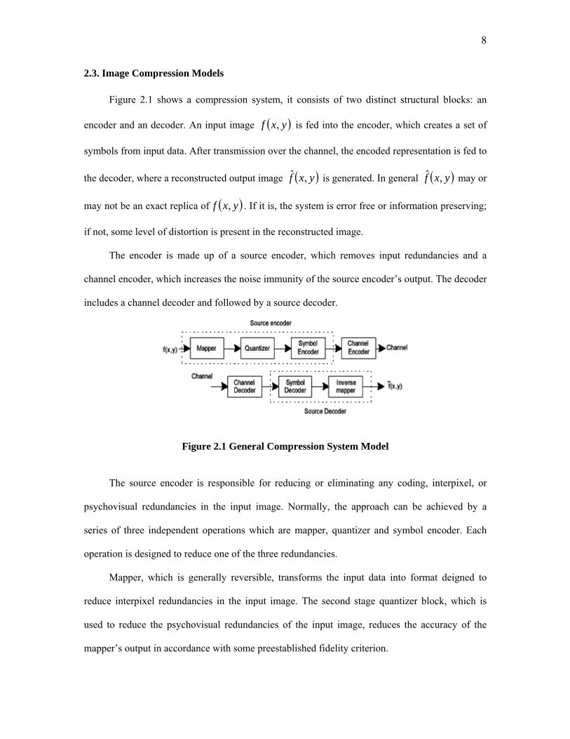
Figure 2.1 shows a compression system, it consists of two distinct structural blocks: an

encoder and an decoder. An input image ( )yxf , is fed into the encoder, which creates a set of

symbols from input data. After transmission over the channel, the encoded representation is fed to

the decoder, where a reconstructed output image ( )yxf ,ˆ is generated. In general ( )yxf ,ˆ may or

may not be an exact replica of ( )yxf , . If it is, the system is error free or information preserving;

if not, some level of distortion is present in the reconstructed image.

The encoder is made up of a source encoder, which removes input redundancies and a

channel encoder, which increases the noise immunity of the source encoder’s output. The decoder

includes a channel decoder and followed by a source decoder.

Figure 2.1 General Compression System Model

The source encoder is responsible for reducing or eliminating any coding, interpixel, or

psychovisual redundancies in the input image. Normally, the approach can be achieved by a

series of three independent operations which are mapper, quantizer and symbol encoder. Each

operation is designed to reduce one of the three redundancies.

Mapper, which is generally reversible, transforms the input data into format deigned to

reduce interpixel redundancies in the input image. The second stage quantizer block, which is

used to reduce the psychovisual redundancies of the input image, reduces the accuracy of the

mapper’s output in accordance with some preestablished fidelity criterion.

9

In the third and final stage of the source encoding process, the symbol coder creates a

fixed- or variable-length code to represent the quantizer output and maps the output in accordance

with the code. It assigns the shortest code words to the most frequently occurring output values

and thus reduces coding redundancy.

On the other hand, source decoder contains only two components, which are symbol

decoder and inverse mapper. These blocks perform, in reverse order, the inverse operations of the

source encoder’s symbol encoder and mapper blocks.

The channel encoder and decoder are designed to reduce the impact of channel noise by

inserting a controlled form of redundancy into the source encoded data. One of the most useful

channel encoding techniques was devised by R.W. Hamming. It is based on appending enough

bits to the data being encoded to ensure that some minimum number of bits must change between

valid code words. The 7-bit Hamming (7, 4) code word 76521 hhhhh K associated with a 4-bit

binary number 0123 bbbb is;

0124

0132

0231

bbbhbbbhbbbh

⊕⊕=⊕⊕=⊕⊕=

07

16

25

33

bhbhbhbh

====

To decode a Hamming encoded result, the channel decoder must check the encoded value

for odd parity over the bit fields in which even parity was previously established. A single-bit

error is indicated by nonzero parity word 124 ccc where

76544

76322

75311

hhhhchhhhchhhhc

⊕⊕⊕=⊕⊕⊕=⊕⊕⊕=

If a nonzero value is found, the decoder simply complements the code word bit position

indicated by the parity word. The decoded binary value is then extracted from the corrected code

word as 7653 hhhh .

10

2.4. Error-Free Compression

Digital images commonly contain lots of redundant information, and thus they are usually

compressed to remove redundancy and minimize the storage space or transport bandwidth. If the

process of redundancy removing is reversible, i.e. the exact reconstruction of the original image

can be achieved, it is called error-free or lossles image compression; otherwise, it is called lossy

image compression. The techniques employed in error-free image compression are all

fundamentally rooted in entropy coding theory and Shannon’s noiseless coding theorem, which

guarantees that as long as the average number of bits per source symbol at the output of the

encoder exceeds the entropy (i.e. average information per symbol) of the data source by an

arbitrarily small amount, the data can be decoded without error.

The problem with current entropy coding algorithms is that the alphabets tend to be large

and thus lead to computationally demanding implementations. A general solution to this problem

is to define several very simple coders that are nearly optimal over a narrow range of sources and

adapt the choices of coder to the statistics of input data. Nowadays, the performances of entropy

coding techniques are very close to its theoretical bound, and thus more research activities

concentrate on decorrelation stage.

For many applications error-free compression is the only acceptable means of data

reduction, such as for documents, text and computer programs. The principle of the error-free

compression strategies normally provides the compression ratios of 2 to 10. Moreover, they are

equally applicable to both binary and gray-scale image. The error-free compression techniques

generally consists of two relatively independent operations: (1) modeling, assign an alternative

representation of the image in which its interpixel redundancies are reduced; and (2) coding,

encode the representation to eliminate coding redundancies. These steps correspond with the

mapping and symbol coding operation of the source coding model.

11

The simplest approach of error-free image compression is to reduce only coding

redundancy. Coding redundancy normally is present in any natural binary encoding of the gray

levels in an image and it can be eliminated by construction of a variable-length code that assigns

the shortest possible code words to the most probable gray levels so that the average length of the

code words is minimized.

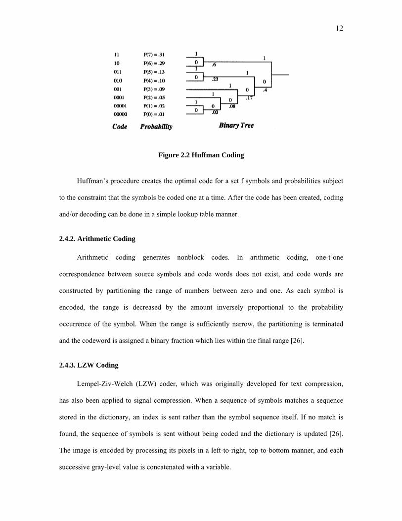
2.4.1. Huffman Coding

Huffman coding is the most popular lossless compression technique. It is a statistical data

compression technique which gives a reduction in the average code length used to represent the

symbols of a alphabet. In fact, it assigns codes to input symbols such that each code length in bits

is approximatively 2log (symbol probability) [12].

When coding the symbols of an information source individually, Huffman coding yields the

smallest possible number of code symbols per source symbols. The first step in Huffman coding

is to create a series of source reductions by ordering the probabilities of the symbols under

consideration and combining the lowest probability symbols under into a single symbol that

replaces them I the next source reduction. Figure 2.2 shows this process for binary coding.

The second step in Huffman’s procedure is to code each reduced source, starting with the

smallest source and working back t the original source.

12

Figure 2.2 Huffman Coding

Huffman’s procedure creates the optimal code for a set f symbols and probabilities subject

to the constraint that the symbols be coded one at a time. After the code has been created, coding

and/or decoding can be done in a simple lookup table manner.

2.4.2. Arithmetic Coding

Arithmetic coding generates nonblock codes. In arithmetic coding, one-t-one

correspondence between source symbols and code words does not exist, and code words are

constructed by partitioning the range of numbers between zero and one. As each symbol is

encoded, the range is decreased by the amount inversely proportional to the probability

occurrence of the symbol. When the range is sufficiently narrow, the partitioning is terminated

and the codeword is assigned a binary fraction which lies within the final range [26].

2.4.3. LZW Coding

Lempel-Ziv-Welch (LZW) coder, which was originally developed for text compression,

has also been applied to signal compression. When a sequence of symbols matches a sequence

stored in the dictionary, an index is sent rather than the symbol sequence itself. If no match is

found, the sequence of symbols is sent without being coded and the dictionary is updated [26].

The image is encoded by processing its pixels in a left-to-right, top-to-bottom manner, and each

successive gray-level value is concatenated with a variable.

13

2.4.4. Bit Plane Coding

Another effective technique for reducing an image’s interpixel redundancies is to process the

image’s bit planes individually. The technique, called bit-plane coding, is based on the concept of

decomposing a multilevel image into a series of binary images and compressing each binary

image via one of several well-known binary compression methods.

2.4.5. Lossless Predictive Coding

In case of Lossless Predictive coding, error-free compression approach does not require

decomposition of an image into a collection of bit planes. This approach is based on eliminating

the interpixel redundancies of closely spaced pixels by extracting and coding only the new

information in each pixel. The new information of a pixel is defined as the difference between the

actual and predicted value of that pixel.

Figure 2.3 shows the basic components of a lossless predictive coding system. The system

consists of encoder and decoder, and an identical predictor.

Figure 2.3 Lossless Predictive Coding Model: encoder, decoder

14

2.5. Lossy compression

Unlike the error-free approaches, lossy encoding is based on concept of compromising the

accuracy of the reconstructed image in exchange for increased compression. If the resulting

distortion can be tolerated, the increase in compression can be significant. The difference between

these two approaches is the presence or absence of the quantizer block.

2.5.1. What Does a Typical Image Coder Look Like in Lossy Compression?

A typical lossy image compression system consists of three closely connected components

namely, Source Encoder (or Linear Transformer), Quantizer, and Entropy Encoder. Compression

is accomplished by applying a linear transform to decorrelate the image data, quantizing the

resulting transform coefficients, and entropy coding the quantized values.

Figure 2.4 A Typical Lossy Signal/Image Encoder

More detailed and complex version of Figure 2.4 is illustrated by Figure 2.5. In Figure 2.5,

a quantizer, that also executes rounding, is now added between the calculation of the prediction

error ne and the symbol encoder. It maps ne to a limited range of values nq and determines both

the amount of extra compression and the deviation of the error-free compression. This happens in

a closed circuit with the predictor to restrict an increase in errors. The predictor does not use

ne but rather nq , because it is known by both the encoder and decoder [27].

15

Figure 2.5 Lossy Predictive Coding Model: encoder and decoder

Here the quantizer, which absorbs the nearest integer function of the error-free encoder, is

inserted between the symbol encoder and the point at which the prediction error is formed.

2.5.2. Transform Coding

In transform coding, a reversible, linear transform is used to map the image into a set of

transform coefficients, which are then quantized and coded. For most natural images, a significant

number of the coefficients have small magnitudes and can be coarsely quantized with little image

distortion.

Next figure illustrates a typical transform coding system. The decoder implements the

inverse sequence of steps of the encoder, which performs four relatively straightforward

operations, which are subimage decomposition, transformation, quantization and coding. The

goal of transformation process is to decorrelate the pixels of each subimage, or to pack as much

information as possible into the smallest number of transform coefficients. The quantization step

then selectively eliminates or more coarsely quantizes the coefficients that carry the least

information. The encoding process terminates by coding the quantized coefficients.

16

Figure 2.6 A Transform Coding System: encoder and decoder

2.5.3. Wavelet Coding

Wavelets are mathematical functions that cut up data into different frequency components,

and then study each component with a resolution matched to its scale. They have advantages over

traditional Fourier methods in analyzing physical situations where the signal contains

discontinuities and sharp spikes. The fundamental idea behind wavelets is to analyze according to

scale. Wavelet algorithms process data at different scales or resolutions. If we look at a signal

with a large "window," we would notice gross features. Similarly, if we look at a signal with a

small "window," we would notice small features.

Before 1930, the main branch of mathematics leading to wavelets began with Joseph

Fourier (1807) with his theories of frequency analysis, now often referred to as Fourier synthesis.

He asserted that any 2π-periodic function f(x) is the sum

( )∑∞

=

++1

0 sincosk

kk kxbkxaa

of its Fourier series. The coefficients a0, ak, and bk are calculated by

( )∫=π

π

2

00 2

1 dxxfa , ( ) ( )∫=π

π

2

0

cos1 dxkxxfak , ( ) ( )∫=π

π

2

0

sin1 dxkxxfbk

After 1807, by exploring the meaning of functions, Fourier series convergence, and

orthogonal systems, mathematicians gradually were led from their previous notion of frequency

analysis to the notion of scale analysis. That is, analyzing f(x) by creating mathematical structures

17

that vary in scale. The first mention of wavelets appeared in an appendix to the thesis of A. Haar

(1909). One property of the Haar wavelet is that it has compact support, which means that it

vanishes outside of a finite interval. Unfortunately, Haar wavelets are not continuously

differentiable which somewhat limits their applications.

Between 1960 and 1980, the mathematicians Guido Weiss and Ronald R. Coifman studied

the simplest elements of a function space, called atoms, with the goal of finding the atoms for a

common function and finding the "assembly rules" that allow the reconstruction of all the

elements of the function space using these atoms. In 1980, Grossman and Morlet, a physicist and

an engineer, broadly defined wavelets in the context of quantum physics. These two researchers

provided a way of thinking for wavelets based on physical intuition.

In 1985, Stephane Mallat gave wavelets an additional jump-start through his work in digital

signal processing. He discovered some relationships between quadrature mirror filters, pyramid

algorithms, and orthonormal wavelet bases (more on these later). Inspired in part by these results,

Y. Meyer constructed the first non-trivial wavelets. Unlike the Haar wavelets, the Meyer wavelets

are continuously differentiable; however they do not have compact support. A couple of years

later, Ingrid Daubechies used Mallat's work to construct a set of wavelet orthonormal basis

functions that are perhaps the most elegant, and have become the cornerstone of wavelet

applications today.

Like the transform coding techniques, wavelet is based on the idea that the coefficients of a

transform that decorrelates the pixels of an image can be coded more efficiently than the original

pixels themselves.

Figure 2.7 shows a typical wavelet coding system. To encode a jj 22 × image, an

analyzing wavelet, ψ, and minimum decomposition level, PJ − , are selected and used to

compute the image’s discrete wavelet transform.

18

Figure 2.7 A Typical Wavelet Coding System: encoder and decoder

If the wavelet has a complimentary scaling function φ, the fast wavelet transform can be

used. Decoding is accomplished by inverting the encoded operations – with the exception of

quantization, which cannot be reserved exactly.

Figure 2.9 Wavelet Transform of the Image “Lena”

Wavelet Selection

Deciding on the optimal wavelet basis to use for image coding is a difficult problem. A

number of design criteria, including smoothness, accuracy of approximation, size of support, and

19

filter frequency selectivity are known to be important. However, the best combination of these

features is not known.

The simplest form of wavelet basis for images is a separable basis formed from translations

and dilations of products of one dimensional wavelets. Using separable transforms reduces the

problem of designing efficient wavelets to a one-dimensional problem, and almost all current

coders employ separable transforms.

The most widely used expansion functions for wavelet-based compression are the

Daubechies wavelets and biorthogonal wavelets. For biorthogonal transforms, the squared error

in the transform domain is not the same as the squared error in the original image [27]. As a

result, the problem of minimizing image error is considerably more difficult than in the

orthogonal case.

Another factor affecting wavelet coding computational complexity and reconstruction error

is the number of transform decomposition levels. Since a P-scale fast wavelet transform involves

P filter bank iterations, the number of operations in the computation of the forward and inverse

transforms increases with the number of decomposition levels. Moreover, quantizing the

increasingly lower-scale coefficients that result with more decomposition levels impacts

increasingly larger areas of the reconstructed image.

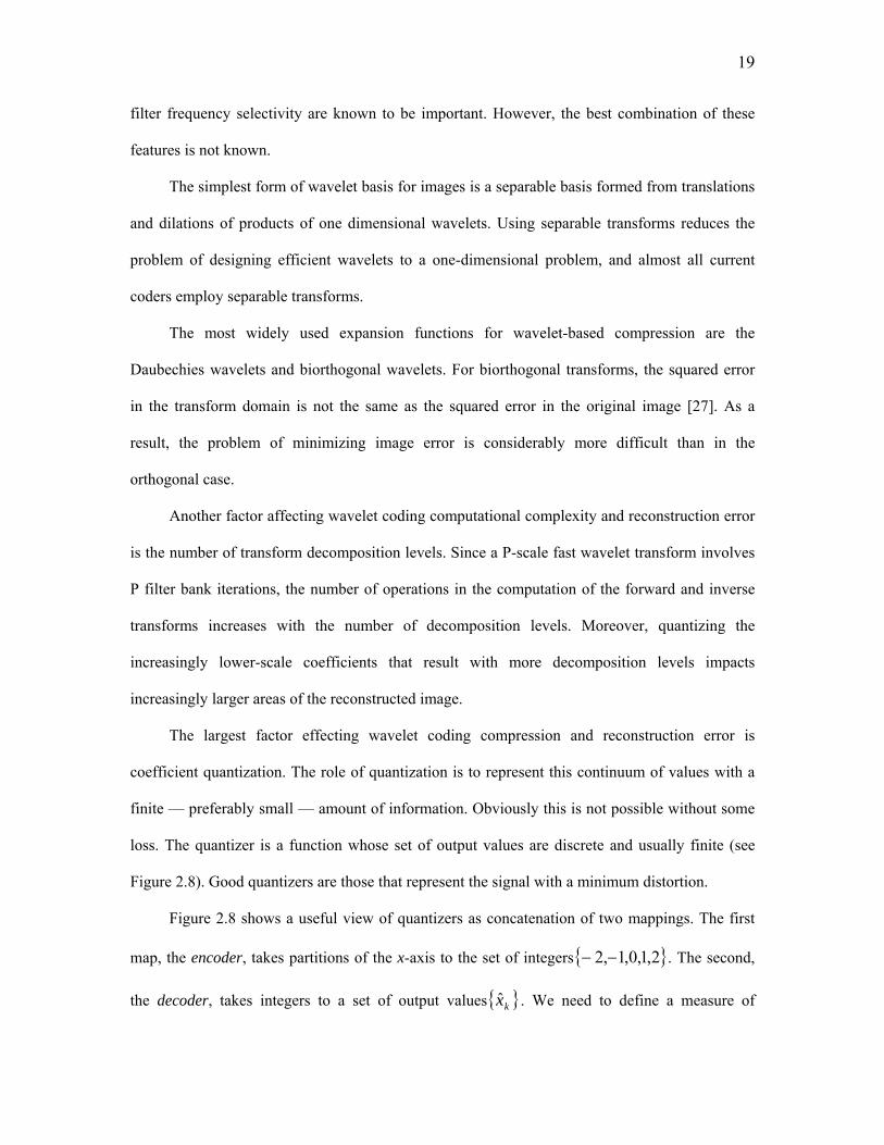
The largest factor effecting wavelet coding compression and reconstruction error is

coefficient quantization. The role of quantization is to represent this continuum of values with a

finite — preferably small — amount of information. Obviously this is not possible without some

loss. The quantizer is a function whose set of output values are discrete and usually finite (see

Figure 2.8). Good quantizers are those that represent the signal with a minimum distortion.

Figure 2.8 shows a useful view of quantizers as concatenation of two mappings. The first

map, the encoder, takes partitions of the x-axis to the set of integers{ }2,1,0,1,2 −− . The second,

the decoder, takes integers to a set of output values{ }kx̂ . We need to define a measure of

20

distortion in order to characterize “good” quantizers. We need to be able to approximate any

possible value of x with an output value.

Figure 2.8 (Left) Quantizer as a function whose output values are discrete. (Right) because

the output values are discrete, a quantizer can be more simply represented only on one axis.

Similarities and Dissimilarities of Wavelet Coding and Transfer Coding

The fast Fourier transform (FFT) and the discrete wavelet transform (DWT) are both linear

operations that generate a data structure that contains n2log segments of various lengths, usually

filling and transforming it into a different data vector of length n2 . Both transforms can be

viewed as a rotation in function space to a different domain. For the FFT, this new domain

contains basis functions that are sines and cosines. For the wavelet transform, this new domain

contains more complicated basis functions called wavelets, mother wavelets, or analyzing

wavelets. Also the basis functions are localized in frequency, making mathematical tools such as

power spectra (how much power is contained in a frequency interval) and scalegrams (to be

defined later) useful at picking out frequencies and calculating power distributions.

The most interesting dissimilarity between these two kinds of transforms is that individual

wavelet functions are localized in space. Fourier sine and cosine functions are not. This

localization feature, along with wavelets' localization of frequency, makes many functions and

operators using wavelets "sparse" when transformed into the wavelet domain. This sparseness, in

21

turn, results in a number of useful applications such as data compression, detecting features in

images, and removing noise from time series.

One way to see the time-frequency resolution differences between the Fourier transform

and the wavelet transform is to look at the basis function coverage of the time-frequency plane.

An advantage of wavelet transforms is that the windows vary. In order to isolate signal

discontinuities, one would like to have some very short basis functions. At the same time, in order

to obtain detailed frequency analysis, one would like to have some very long basis functions. A

way to achieve this is to have short high-frequency basis functions and long low-frequency ones.

This happy medium is exactly what you get with wavelet transforms.

One thing to remember is that wavelet transforms do not have a single set of basis functions

like the Fourier transform, which utilizes just the sine and cosine functions. Instead, wavelet

transforms have an infinite set of possible basis functions. Thus wavelet analysis provides

immediate access to information that can be obscured by other time-frequency methods such as

Fourier analysis.

2.6. Image Compression Standards

Many of the lossy and error-free compression methods play important roles in popular

image compression standards. Most of the standards are approved by the International

Standardization Organization (ISO) and the consultative Committee of the International

Telephone and Telegraph (CCITT). They address both binary and continuous-tone image

compression, as well as both still-frame and video applications.

2.6.1. Binary Image Compression Standards

Two of the most widely used image compression standards are the CCITT Group 3 and 4

standards for binary image compression. Despite of being currently utilized in a wide variety of

computer applications, they were originally designed as FAX coding methods for transmitting

22

documents over telephone networks. Both standards use the same nonadaptive 2-D coding

approach.

Since the Group 3 and 4 standards are based on nonadaptive techniques, however, they

sometimes result in data expansions. To overcome this and related problems, the Joint Bilevel

Imaging Group (JBIG) has adopted and/or proposed several other binary compression standards,

such as JBIG1 and JBIG2.

2.6.2. Continuous Tone Still Image Compression Standards

The CCITT and ISO have defined several continuous tone image compression standards.

These standards addresses both monochrome and color image compression. In contrast to binary

compression standards, continuous tone standards are based principally on the lossy transform

coding techniques. The most well known still image compression standards are DCT-based JPEG

standard and the recently proposed wavelet-based JPEG-2000 standard.

JPEG defines three different coding systems. First one is a lossy baseline coding system,

which is based on the DCT and is adequate for most compression applications. Second one is an

extended coding system for greater compression, higher precision or progressive reconstruction

applications, and the last one is a lossless independent coding system for reversible compression.

Detailed information about JPEG standard will be given in next chapter.

On the other hand, although not yet formally adopted, JPEG 2000 extends the initial JPEG

standard to provide increased flexibility in both the compression of continuous tone still images

and access to the compressed data. The standard is based on the wavelet coding techniques.

Coefficient quantization is adapted to individual scales and subbands and the quantized

coefficients are arithmetically coded on a bit-plane basis.

23

2.6.3. Video Compression Standards

Video compression standards extend the transform-based, still image compression

techniques of the previous section to include methods for reducing temporal or frame-to-frame

redundancies. Depending on the intended application, the standards can be grouped into two

broad categories, which are video teleconferencing standards and multimedia standards. Each

video teleconferencing standard uses a motion-compensated, DCT-based coding scheme.

Multimedia video compression standards for video use also similar motion estimation and coding

techniques.

24

CHAPTER 3: INTRODUCTION TO GPU

The rapid increase in the performance of graphics hardware, coupled with recent

improvements in its programmability, have made graphics hardware a compelling platform for

computationally demanding tasks in a wide variety of application domains. GPGPU stands for

General-Purpose computation on GPUs. With the increasing programmability of commodity

graphics processing units (GPUs), these chips are capable of performing more than the specific

graphics computations for which they were designed. They are now capable coprocessors, and

their high speed makes them useful for a variety of applications. Traditionally, graphics hardware

has been optimized for a fixed functionality rendering pipeline that implements only the simple

Phong lighting model, and rendering computation has been restricted to 8-bit fixed-point

precision. Today’s GPUs have evolved into powerful and flexible streaming processors with fully

programmable floating-point pipelines and tremendous aggregate computational power and

memory bandwidth [25].

3.1. Why GPGPU?

First reason is they are Powerful and Inexpensive. Not only is current graphics hardware

fast, it is accelerating quickly and graphics hardware performance is roughly doubling every six

months. Why is the performance of graphics hardware increasing more rapidly than that of

CPUs? The disparity in performance can be attributed to fundamental architectural differences:

CPUs are optimized for high performance on sequential code, so many of their transistors are

dedicated to supporting non-computational tasks like branch prediction and caching. On the other

hand, the highly parallel nature of graphics computations enables GPUs to use additional

transistors for computation, achieving higher arithmetic intensity with the same transistor count.

Second important reason is that GPUs are flexible and programmable. Modern graphics

architectures have become flexible as well as powerful. Once fixed-function pipelines capable of

25

outputting only 8-bit-per-channel color values, modern GPUs include fully programmable

processing units that support vectorized floating-point operations at full IEEE single precision.

On the other hand it has its own limitations and difficulties. The GPU is hardly a

computational panacea. The arithmetic power of the GPU is a result of its highly specialized

architecture, evolved over the years to extract the maximum performance on the highly parallel

tasks of traditional computer graphics. Today’s GPUs also lack some fundamental computing

constructs, such as integer data operands. The lack of integers and associated operations such as

bit-shifts and bitwise logical operations (AND, OR, XOR, NOT) makes GPUs ill-suited for many

computationally intense tasks such as cryptography. Finally, while the recent increase in precision

to 32-bit floating point has enabled a host of GPGPU applications; 64-bit double precision

arithmetic appears to be on the distant horizon at best. The lack of double precision hampers or

prevents GPUs from being applicable to many very large-scale computational science problems.

GPGPU computing presents challenges even for problems that map well to the GPU, because

despite advances in programmability and high-level languages, graphics hardware remains

difficult to apply to non-graphics tasks.

3.2. Overview of Programmable Graphics Hardware

3.2.1 Overview of the Graphics Pipeline

The application domain of interactive 3D graphics has several characteristics that

differentiate it from more general computation domains. In particular, interactive 3D graphics

applications require high computation rates and exhibit substantial parallelism. Building custom

hardware that takes advantage of the native parallelism in the application, then, allows higher

performance on graphics applications than can be obtained on more traditional microprocessors.

All of today’s commodity GPUs structure their graphics computation in a similar

organization called the graphics pipeline. This pipeline is designed to allow hardware

implementations to maintain high computation rates through parallel execution. The pipeline is

26

divided into several stages; all geometric primitives pass through every stage. In hardware, each

stage is implemented as a separate piece of hardware on the GPU in what is termed a task-

parallel machine organization. Figure 3.1 shows the pipeline stages in current GPUs.

Figure 3.1 The modern graphics hardware pipeline. The vertex and fragment processor

stages are both programmable by the user.

The input to the pipeline is a list of geometry, expressed as vertices in object coordinates;

the output is an image in a framebuffer. The first stage of the pipeline, the geometry stage,

transforms each vertex from object space into screen space, assembles the vertices into triangles,

and traditionally performs lighting calculations on each vertex. The output of the geometry stage

is triangles in screen space.

The next stage, rasterization, both determines the screen positions covered by each triangle

and interpolates per-vertex parameters across the triangle. The result of the rasterization stage is a

fragment for each pixel location covered by a triangle. The third stage, the fragment stage,

computes the color for each fragment, using the interpolated values from the geometry stage. This

computation can use values from global memory in the form of textures; typically the fragment

stage generates addresses into texture memory, fetches their associated texture values, and uses

them to compute the fragment color. In the final stage, composition, fragments are assembled into

an image of pixels, usually by choosing the closest fragment to the camera at each pixel location.

27

3.2.2 Programmable Hardware

As graphics hardware has become more powerful, one of the primary goals of each new

generation of GPU has been to increase the visual realism of rendered images. The graphics

pipeline was historically a fixed-function pipeline, where the limited number of operations

available at each stage of the graphics pipeline was hardwired for specific tasks [18].

Over the past six years, graphics vendors have transformed the fixed-function pipeline into a

more flexible programmable pipeline. This effort has been primarily concentrated on two stages

of the graphics pipeline: the geometry stage and the fragment stage. In the fixed-function

pipeline, the geometry stage included operations on vertices such as transformations and lighting

calculations. In the programmable pipeline, these fixed-function operations are replaced with a

user-defined vertex program. Similarly, the fixed-function operations on fragments that determine

the fragment’s color are replaced with a user-defined fragment program.

1999 marked the introduction of the first programmable stage, NVIDIA’s register combiner

operations that allowed a limited combination of texture and interpolated color values to compute

a fragment color. In 2002, ATI’s Radeon 9700 led the transition to floating-point computation in

the fragment pipeline. The vital step for enabling general-purpose computation on GPUs was the

introduction of fully programmable hardware and an assembly language for specifying programs

to run on each vertex [LKM01] or fragment. This programmable shader hardware is explicitly

designed to process multiple data-parallel primitives at the same time. As of 2005, the vertex

shader and pixel shader standards are both in their third revision. The instruction sets of each

stage are limited compared to CPU instruction sets; they are primarily math operations, many of

which are graphics-specific. The newest addition to the instruction sets of these stages has been

limited control flow operations.

In general, these programmable stages input a limited number of 32-bit floating-point 4-

vectors. The vertex stage outputs a limited number of 32-bit floating-point 4-vectors that will be

28

interpolated by the rasterizer; the fragment stage outputs up to 4 floating-point 4-vectors,

typically colors. Each programmable stage can access constant registers across all primitives and

also read-write registers per primitive. The programmable stages have limits on their numbers of

inputs, outputs, constants, registers, and instructions; with each new revision of the vertex shader

and pixel [fragment] shader standard, these limits have increased. GPUs typically have multiple

vertex and fragment processors. Fragment processors have the ability to fetch data from textures,

so they are capable of memory gather. However, the output address of a fragment is always

determined before the fragment is processed—the processor cannot change the output location of

a pixel—so fragment processors are incapable of memory scatter. Vertex processors recently

acquired texture capabilities, and they are capable of changing the position of input vertices,

which ultimately affects where in the image pixels will be drawn. Thus, vertex processors are

capable of both gather and scatter. Unfortunately, vertex scatter can lead to memory and

rasterization coherence issues further down the pipeline. Combined with the lower performance

of vertex processors, this limits the utility of vertex scatter in current GPUs.

3.2.3. Introduction to the GPU Programming Model

GPUs achieve high performance through data parallelism, which requires a programming

model distinct from the traditional CPU sequential programming model. The stream

programming model exposes the parallelism and communication patterns inherent in the

application by structuring data into streams and expressing computation as arithmetic kernels that

operate on streams.

Because typical scenes have more fragments than vertices, in modern GPUs the

programmable stage with the highest arithmetic rates is the fragment processor. A typical GPGPU

program uses the fragment processor as the computation engine in the GPU. Such a program is

structured as follows; first of all, the programmer determines the data-parallel portions of his

application. The application must be segmented into independent parallel sections. Each of these

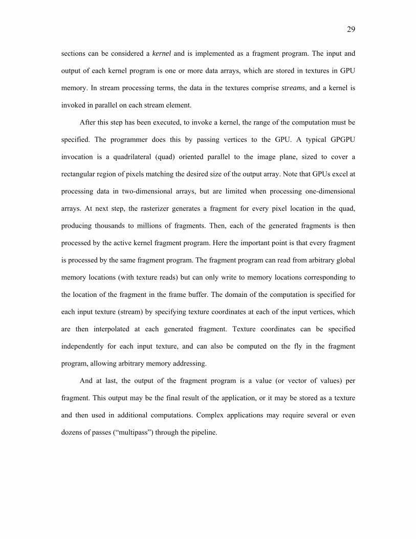
29

sections can be considered a kernel and is implemented as a fragment program. The input and

output of each kernel program is one or more data arrays, which are stored in textures in GPU

memory. In stream processing terms, the data in the textures comprise streams, and a kernel is

invoked in parallel on each stream element.

After this step has been executed, to invoke a kernel, the range of the computation must be

specified. The programmer does this by passing vertices to the GPU. A typical GPGPU

invocation is a quadrilateral (quad) oriented parallel to the image plane, sized to cover a

rectangular region of pixels matching the desired size of the output array. Note that GPUs excel at

processing data in two-dimensional arrays, but are limited when processing one-dimensional

arrays. At next step, the rasterizer generates a fragment for every pixel location in the quad,

producing thousands to millions of fragments. Then, each of the generated fragments is then

processed by the active kernel fragment program. Here the important point is that every fragment

is processed by the same fragment program. The fragment program can read from arbitrary global

memory locations (with texture reads) but can only write to memory locations corresponding to

the location of the fragment in the frame buffer. The domain of the computation is specified for

each input texture (stream) by specifying texture coordinates at each of the input vertices, which

are then interpolated at each generated fragment. Texture coordinates can be specified

independently for each input texture, and can also be computed on the fly in the fragment

program, allowing arbitrary memory addressing.

And at last, the output of the fragment program is a value (or vector of values) per

fragment. This output may be the final result of the application, or it may be stored as a texture

and then used in additional computations. Complex applications may require several or even

dozens of passes (“multipass”) through the pipeline.

30

3.2.4. GPU Program Flow Control

Flow control is a fundamental concept in computation. Branching and looping are such basic

concepts that it can be daunting to write software for a platform that supports them to only a

limited extent. The latest GPUs support vertex and fragment program branching in multiple

forms, but their highly parallel nature requires care in how they are used. This section surveys

some of the limitations of branching on current GPUs and describes a variety of techniques for

iteration and decision-making in GPGPU programs.

There are three basic implementations of data-parallel branching in use on current GPUs

which are named as predication, MIMD branching, and SIMD branching. Architectures that

support only predication do not have true data-dependent branch instructions. Instead, the GPU

evaluates both sides of the branch and then discards one of the results based on the value of the

Boolean branch condition. The disadvantage of predication is that evaluating both sides of the

branch can be costly, but not all current GPUs have true data-dependent branching support. The

compiler for high-level shading languages like Cg or the OpenGL Shading Language

automatically generates predicated assembly language instructions if the target GPU supports

only predication for flow control.

In Multiple Instruction Multiple Data (MIMD) architectures that support branching, different

processors can follow different paths through the program. In Single Instruction Multiple Data

(SIMD) architectures, all active processors must execute the same instructions at the same time.

The only MIMD processors in a current GPU are the vertex processors of the NVIDIA GeForce 6

and NV40 Quadro GPUs. All current GPU fragment processors are SIMD. In SIMD, when

evaluation of the branch condition is identical on all active processors, only the taken side of the

branch must be evaluated, but if one or more of the processors evaluates the branch condition

differently, then both sides must be evaluated and the results predicated. As a result, divergence

in the branching of simultaneously processed fragments can lead to reduced performance.

31

Because explicit branching can hamper performance on GPUs, it is useful to have multiple

techniques to reduce the cost of branching. A useful strategy is to move flow-control decisions up

the pipeline to an earlier stage where they can be more efficiently evaluated.

On the GPU, as on the CPU, avoiding branching inside inner loops is beneficial. On the

GPU, the computation is divided into two fragment programs: one for interior cells and one for

boundary cells. The interior program is applied to the fragments of a quad drawn over all but the

outer one-pixel edge of the output buffer. The boundary program is applied to fragments of lines

drawn over the edge pixels.

3.3. Programming Systems

Successful programming requires at least three basic components: a high-level language for

code development, a debugging environment, and profiling tools. CPU programmers have a large

number of well-established languages, debuggers, and profilers to choose from when writing

applications. Conversely, GPU programmers have just a small handful of languages to choose

from, and few if any full-featured debuggers and profilers.

Most high-level GPU programming languages today share one thing in common: they are

designed around the idea that GPUs generate pictures. As such, the high-level programming

languages are often referred to as shading languages. That is, they are a high-level language that

compiles into a vertex shader and a fragment shader to produce the image described by the

program.

Cg, HLSL, and the OpenGL Shading Language all abstract the capabilities of the

underlying GPU and allow the programmer to write GPU programs in a more familiar C-like

programming language. They do not stray far from their origins as languages designed to shade

polygons. All retain graphics-specific constructs: vertices, fragments, textures, etc. Cg and HLSL

provide abstractions that are very close to the hardware, with instruction sets that expand as the

underlying hardware capabilities expand. The OpenGL Shading Language was designed looking

32

a bit further out, with many language features (e.g. integers) that do not directly map to hardware

available today.

Sh is a shading language implemented on top of C++. Sh provides a shader algebra for

manipulating and defining procedurally parameterized shaders. Sh manages buffers and textures,

and handles shader partitioning into multiple passes.

At last, Ashli works at a level one step above that of Cg, HLSL, or the OpenGL Shading

Language. Ashli reads as input shaders written in HLSL, the OpenGL Shading Language, or a

subset of RenderMan. Ashli then automatically compiles and partitions the input shaders to run

on a programmable GPU.

Looking up data from memory is done by issuing a texture fetch. The GPGPU program

may conceptually have nothing to do with drawing geometric primitives and fetching textures, yet

the shading languages described in the previous section force the GPGPU application writer to

think in terms of geometric primitives, fragments, and textures. Instead, GPGPU algorithms are

often best described as memory and math operations, concepts much more familiar to CPU

programmers. Here are some programming systems that attempt to provide GPGPU functionality

while hiding the GPU-specific details from the programmer.

The Brook programming language extends ANSI C with concepts from stream

programming. Brook can use the GPU as a compilation target. Brook streams are conceptually

similar to arrays, except all elements can be operated on in parallel. Kernels are the functions that

operate on streams. Brook automatically maps kernels and streams into fragment programs and

texture memory.

Scout is a GPU programming language designed for scientific visualization. Scout allows

runtime mapping of mathematical operations over data sets for visualization.

Finally, the Glift template library provides a generic template library for a wide range of

GPU data structures. It is designed to be a stand-alone GPU data structure library that helps

33

simplify data structure design and separate GPU algorithms from data structures. The library

integrates with a C++, Cg, and OpenGL GPU development environment.

One of the most important tools needed for successful platforms is a debugger. Until

recently, support for debugging on GPUs was fairly limited. The needs of a debugger for GPGPU

programming are very similar to what traditional CPU debuggers provide, including variable

watches, program break points, and single step execution. GPU programs often involve user

interaction. While a debugger does not need to run the application at full speed, the application

being debugged should maintain some degree of interactivity. A GPU debugger should be easy to

add to and remove from an existing application, should mangle GPU state as little as possible,

and should execute the debug code on the GPU, not in a software rasterizer. Finally, a GPU

debugger should support the major GPU programming APIs and vendor-specific extensions.

A GPU debugger has a challenge in that it must be able to provide debug information for

multiple vertices or pixels at a time. There are a few different systems for debugging GPU

programs available to use, but nearly all are missing one or more of the important features.

gDEBugger and GLIntercept [Tre05] are tools designed to help debug OpenGL programs. Both

are able to capture and log OpenGL state from a program. gDEBugger allows a programmer to

set breakpoints and watch OpenGL state variables at runtime. There is currently no specific

support for debugging shaders. GLIntercept does provide runtime shader editing, but again is

lacking in shader debugging support.

The Microsoft Shader Debugger, however, does provide runtime variable watches and

breakpoints for shaders. Unfortunately, debugging requires the shaders to be run in software

emulation rather than on the hardware. While many of the tools mentioned so far provide a lot of

useful features for debugging, none provide any support for shader data visualization or printf-

style debugging. The Image Debugger was among the first tools to provide this functionality by

providing a printf-like function over a region of memory. The region of memory gets mapped to a

display window, allowing a programmer to visualize any block of memory as an image. Also, the

34

Shadesmith Fragment Program Debugger was the first system to automate printf-style debugging

while providing basic shader debugging functionality like breakpoints and stepping. Finally,

Duca et al. have recently described a system that not only provides debugging for graphics state

but also both vertex and fragment programs.

3.4. GPGPU Techniques

We already knew that stream programming model is a useful abstraction for programming

GPUs. There are several fundamental operations on streams that many GPGPU applications

implement as a part of computing their final results: map, reduce, scatter and gather, stream

filtering, sort, and search.

Given a stream of data elements and a function, map will apply the function to every element in

the stream. The GPU implementation of map is straightforward. The result of the fragment

program execution is the result of the map operation.

Sometimes a computation requires computing a smaller stream from a larger input stream,

possibly to a single element stream. This type of computation is called a reduction. On GPUs,

reductions can be performed by alternately rendering to and reading from a pair of textures. On

each rendering pass, the size of the output, the computational range, is reduced by one half. In

general, we can compute a reduction over a set of data in ( )nO log steps using the parallel GPU

hardware, compared to ( )nO steps for a sequential reduction on the CPU. For a two-dimensional

reduction, the fragment program reads four elements from four quadrants of the input texture, and

the output size is halved in both dimensions at each step.

Two fundamental memory operations with which most programmers are familiar are write

and read. If the write and read operations access memory indirectly, they are called scatter and

gather respectively. A scatter operation looks like the C code d[a] = v where the value v is being

stored into the data array d at address a. A gather operation is just the opposite of the scatter

operation. The C code for gather looks like v = d[a].

35

The GPU implementation of gather is essentially a dependent texture fetch operation.

Unfortunately, scatter is not as straightforward to implement. Fragments have an implicit

destination address associated with them: their location in frame buffer memory. A scatter

operation would require that a program change the frame buffer write location of a given

fragment, or would require a dependent texture write operation.

A sort operation allows us to transform an unordered set of data into an ordered set of data.

Sorting is a classic algorithmic problem that has been solved by several different techniques on

the CPU. Unfortunately, nearly all of the classic sorting methods are not applicable to a clean

GPU implementation. The main reason these algorithms are not GPU friendly. Classic sorting

algorithms are data-dependent and generally require scatter operations. Most GPU-based sorting

implementations have been based on sorting networks. The main idea behind a sorting network is

that a given network configuration will sort input data in a fixed number of steps, regardless of

the input data. Additionally, all the nodes in the network have a fixed communication path. The

fixed communication pattern means the problem can be stated in terms of gather rather than a

scatter, and the fixed number of stages for a given input size means the sort can be implemented

without data-dependent branching. This yields an efficient GPU-based sort, with an O(n log2 n)

complexity. Sorting networks can also be implemented efficiently using the texture mapping and

blending functionalities of the GPU.

The last stream operation, search, allows us to find a particular element within a stream.

Search can also be used to find the set of nearest neighbors to a specified element. Nearest

neighbor search is used extensively when computing radiance estimates in photon mapping and in

database queries. The simplest form of search is the binary search. This is a basic algorithm,

where an element is located in a sorted list in ( )nO log time. Binary search works by comparing

the center element of a list with the element being searched for. The GPU implementation of

binary search is a straightforward mapping of the standard CPU algorithm to the GPU. Binary

36

search is inherently serial, so we can not parallelize lookup of a single element. Nearest neighbor

search is a slightly more complicated form of search. In this search, we want to find the k nearest

neighbors to a given element. On the CPU, this has traditionally been done using a k-d tree.

Unfortunately, the GPU implementation of nearest neighbor search is not as straightforward. We

can search a k-d tree data structure, but we have not yet found a way to efficiently maintain a

priority queue. The important detail about the priority queue is that candidate neighbors can be

removed from the queue if closer neighbors are found.

3.4.1. Data Structures

Effective GPGPU data structures must support fast and coherent parallel accesses as well as

efficient parallel iteration, and must also work within the constraints of the GPU memory model.

Before describing GPGPU data structures, let’s briefly describe the memory primitives with

which they are built. To maintain parallelism, operations on these textures are limited to read-

only or write-only access within a kernel. Write access is further limited by the lack of scatter

support. Outside of kernels, users may allocate or delete textures, copy data between the CPU and

GPU, copy data between GPU textures, or bind textures for kernel access. Lastly, most GPGPU

data structures are built using 2D textures for two reasons. First, the maximum 1D texture size is

often too small to be useful and second, current GPUs cannot efficiently write to a slice of a 3D

texture. C/C++ programming, algorithms are defined in terms of iteration over the elements of a

data structure. Iteration over a dense set of elements is usually accomplished by drawing a single

large quad. This is the computation model supported by Brook, Sh, and Scout. Complex

structures, however, such as sparse arrays, adaptive arrays, and grid-of-list structures often

require more complex iteration constructs. These range iterators are usually defined using

numerous smaller quads, lines, or point sprites. The majority of data structures used thus far in

GPGPU programming are random-access multidimensional containers, including dense arrays,

sparse arrays, and adaptive arrays. In order to provide programmers with the abstraction of

37

iterating over elements in the virtual domain, GPGPU data structures must support both virtual-

to-physical and physical-to-virtual address translation.

The most common GPGPU data structure is a contiguous multidimensional array. These

arrays are often implemented by first mapping from N-D to 1D, then from 1D to 2D. Iteration

over dense arrays is performed by drawing large quads that span the range of elements requiring

computation. Brook, Glift, and Sh provide users with fully virtualized CPU/GPU interfaces to

these structures.

Sparse arrays are multidimensional structures that store only a subset of the grid elements

defined by their virtual domain. Static Sparse Arrays can use complex, pre-computed packing

schemes to represent the active elements because the structure does not change. We define static

to mean that the number and position of stored (non-zero) elements does not change throughout

GPU computation, although the GPU computation may update the value of the stored elements. A

common application of static sparse arrays is sparse matrices. Dynamic sparse arrays are similar

to static sparse arrays but support insertion and deletion of non-zero elements during GPU

computation. An example application for a dynamic sparse array is the data structure for a

deforming implicit surface. Multidimensional page table address translators are an attractive

option for dynamic sparse (and adaptive) arrays because they provide fast data access and can be

easily updated.

Adaptive arrays are a generalization of sparse arrays and represent structures such as

quadtrees, octrees, kNN-grids, and k-d trees. These structures non-uniformly map data to the

virtual domain and are useful for very sparse or multiresolution data. Similar to their CPU

counterparts, GPGPU adaptive address translators are represented with a tree, a page table, or a

hash table. There are two types of adaptive arrays which are named as Static Adaptive arrays and

Dynamic Adaptive arrays.

GPGPU technique Differential equations arise in many disciplines of science and

engineering. Their efficient solution is necessary for everything from simulating physics for

38

games to detecting features in medical imaging. Typically differential equations are solved for

entire arrays of input. There are two main classes of differential equations: ordinary differential

equations (ODEs) and partial differential equations (PDEs). An ODE is an equality involving a

function and its derivatives. PDEs, on the other hand, are equations involving functions and their

partial derivatives, like the wave equation. ODEs typically arise in the simulation of the motion of

objects, and this is where GPUs have been applied to their solution.

3.5. GPGPU Applications

The use of computer graphics hardware for general-purpose computation has been an area

of active research for many years. Pixar’s Chap was one of the earliest processors to explore a

programmable SIMD computational organization, on 16-bit integer data. These early graphics

computers were typically graphics compute servers rather than desktop workstations.

The wide deployment of GPUs in the last several years has resulted in an increase in

experimental research with graphics hardware. The earliest work on desktop graphics processors

used non-programmable (“fixed-function”) GPUs. Programmability in GPUs first appeared in the

form of vertex programs combined with a limited form of fragment programmability via

extensive user-configurable texture addressing and blending operations. A major limitation of this

generation of GPUs was the lack of floating-point precision in the fragment processors.

3.5.1. Physically-Based Simulation

Early GPU-based physics simulations used cellular techniques such as cellular automata

(CA). Full floating point support in GPUs has enabled the next step in physically-based

simulation: finite difference and finite element techniques for the solution of systems of partial

differential equations (PDEs). Spring-mass dynamics on a mesh were used to implement basic

cloth simulation on a GPU. Several researchers have also implemented particle system simulation

on GPUs. Several groups have used the GPU to successfully simulate fluid dynamics. Related to

39

fluid simulation is the visualization of flows, which has been implemented using graphics

hardware to accelerate line integral convolution and Lagrangian-Eulerian advection.

3.5.2. Signal and Image Processing

The high computational rates of the GPU have made graphics hardware an attractive target

for demanding applications such as those in signal and image processing. The segmentation

problem seeks to identify features embedded in 2D or 3D images. A driving application for

segmentation is medical imaging. A common problem in medical imaging is to identify a 3D

surface embedded in a volume image obtained with an imaging technique such as Magnetic

Resonance Imaging (MRI) or Computed Tomograph (CT) Imaging. Fully automatic

segmentation is an unsolved image processing research problem. Semi-automatic methods,

however, offer great promise by allowing users to interactively guide image processing

segmentation computations. GPGPU segmentation approaches have made a significant

contribution in this area by providing speedups of more than 10× and coupling the fast

computation to an interactive volume renderer.

40

CHAPTER 4: FAST COMPRESSION TECHNIQUES

Some of the most common techniques that are used for image compression are JPEG image

compression which DCT/IDCT [5] based image coding standard, Cellular Neural Networks [22],

and fractal image compression [10, 30]. In most cases, image compression has to be processed in

Real-Time. Unfortunately, the large amount of computation required by classical image

compression algorithms prohibits the use of common sequential processors. On the other hand

VLSI dedicated architectures have a main drawback of the impossibility of adaptation to the

image to be treated. To solve this problem, a new parallel image compression algorithm is

introduced which is able to be implemented on either SIMD or MIMD architecture [21]. It has

been shown that compression algorithms based on Wavelet Transform, Vector quantization and

Huffman Coding provide one of the best trade-off between compression rates and quality.

4.1. JPEG: DCT-Based Image Coding Standard

The JPEG process is a widely used form of lossy image compression that centers on the

Discrete Cosine Transform. The idea of compressing an image is not new. The discrete cosine

transform (DCT) is a technique for converting a signal into elementary frequency components. It

works by separating images into parts of differing frequencies. During compression step, the less

important frequencies are discarded, hence the use of the term “lossy”. Then, only the most

important frequencies that remain are used retrieve the image in the decompression process.

It is widely used in image compression. Developed by Ahmed, Natarajan, and Rao [1974],

the DCT is a close relative of the discrete Fourier transform (DFT). Its application to image

compression was pioneered by Chen and Pratt [1984]. The discovery of DCT in 1974 is an

important achievement for the research community working on image compression. It is a close

relative of DFT, a technique for converting a signal into elementary frequency components. Thus

DCT can be computed with a Fast Fourier Transform (FFT) like algorithm in ( )nnO log

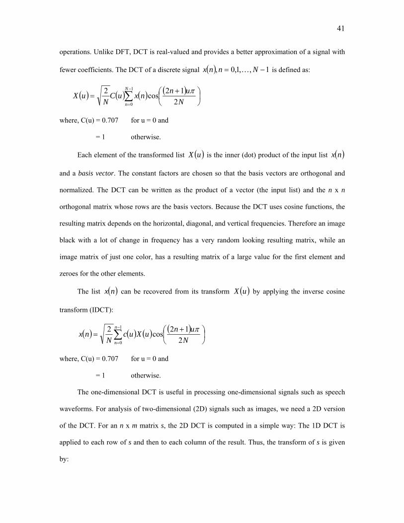
41

operations. Unlike DFT, DCT is real-valued and provides a better approximation of a signal with

fewer coefficients. The DCT of a discrete signal ( ) 1,,1,0, −= Nnnx K is defined as:

( ) ( ) ( ) ( )∑−

=⎟⎠⎞

⎜⎝⎛ +

=1

0 212cos2 N

n NunnxuC

NuX π

where, C(u) = 0.707 for u = 0 and

= 1 otherwise.

Each element of the transformed list ( )uX is the inner (dot) product of the input list ( )nx

and a basis vector. The constant factors are chosen so that the basis vectors are orthogonal and

normalized. The DCT can be written as the product of a vector (the input list) and the n x n

orthogonal matrix whose rows are the basis vectors. Because the DCT uses cosine functions, the

resulting matrix depends on the horizontal, diagonal, and vertical frequencies. Therefore an image

black with a lot of change in frequency has a very random looking resulting matrix, while an

image matrix of just one color, has a resulting matrix of a large value for the first element and

zeroes for the other elements.

The list ( )nx can be recovered from its transform ( )uX by applying the inverse cosine

transform (IDCT):

( ) ( ) ( ) ( )∑−

=⎟⎠⎞

⎜⎝⎛ +

=1

0 212cos2 n

n NunuXuc

Nnx π

where, C(u) = 0.707 for u = 0 and

= 1 otherwise.

The one-dimensional DCT is useful in processing one-dimensional signals such as speech

waveforms. For analysis of two-dimensional (2D) signals such as images, we need a 2D version

of the DCT. For an n x m matrix s, the 2D DCT is computed in a simple way: The 1D DCT is

applied to each row of s and then to each column of the result. Thus, the transform of s is given

by:

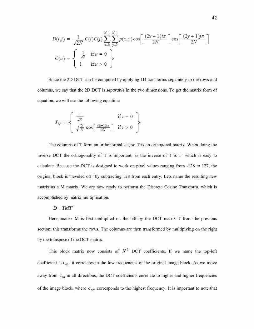
42

Since the 2D DCT can be computed by applying 1D transforms separately to the rows and

columns, we say that the 2D DCT is separable in the two dimensions. To get the matrix form of

equation, we will use the following equation:

The columns of T form an orthonormal set, so T is an orthogonal matrix. When doing the

inverse DCT the orthogonality of T is important, as the inverse of T is T` which is easy to

calculate. Because the DCT is designed to work on pixel values ranging from -128 to 127, the

original block is “leveled off” by subtracting 128 from each entry. Lets name the resulting new

matrix as a M matrix. We are now ready to perform the Discrete Cosine Transform, which is

accomplished by matrix multiplication.

TTMD ′=

Here, matrix M is first multiplied on the left by the DCT matrix T from the previous

section; this transforms the rows. The columns are then transformed by multiplying on the right

by the transpose of the DCT matrix.

This block matrix now consists of 2N DCT coefficients. If we name the top-left

coefficient as 00c , it correlates to the low frequencies of the original image block. As we move

away from 00c in all directions, the DCT coefficients correlate to higher and higher frequencies

of the image block, where NNc corresponds to the highest frequency. It is important to note that

43

the human eye is most sensitive to low frequencies, and results from the quantization step will

reflect this fact.

In 1992, JPEG established the first international standard for still image compression where

the encoders and decoders are DCT-based. The JPEG standard specifies three modes namely

sequential, progressive, and hierarchical for lossy encoding, and one mode of lossless encoding

[28].

Key processing steps in such an encoder and decoder for grayscale images are shown

below figures. Color image compression can be approximately regarded as compression of

multiple grayscale images, which are either compressed entirely one at a time, or are compressed

by alternately interleaving 8x8 sample blocks from each in turn.

Figure 4.1 JPEG Encoder Block Diagram

Figure 4.2 JPEG Decoder Block Diagram

The DCT-based encoder can be thought of as essentially compression of a stream of 8x8

blocks of image samples. Each 8x8 block makes its way through each processing step, and yields

44

output in compressed form into the data stream. Because adjacent image pixels are highly

correlated, the “forward” DCT (FDCT) processing step lays the foundation for achieving data

compression by concentrating most of the signal in the lower spatial frequencies. For a typical

8x8 sample block from a typical source image, most of the spatial frequencies have zero or near-

zero amplitude and need not be encoded. In principle, the DCT introduces no loss to the source

image samples; it merely transforms them to a domain in which they can be more efficiently

encoded.

After output from the FDCT, each of the 64 DCT coefficients is uniformly quantized in

conjunction with a carefully designed 64-element Quantization Table (QT). Quantization is the

process of reducing the number of possible values of a quantity, thereby reducing the number of

bits needed to represent it. Quantization is achieved by dividing each element in the transformed

image matrix D by the corresponding element in the quantization matrix, and then rounding to the

nearest integer value.

⎟⎟⎠

⎞⎜⎜⎝

⎛=

ji

jiji Q

DroundC

,

,,

On the other hand Dequantization, which maps the quantized value back into its original

range (but not its original precision), is achieved by multiplying the value by the weight. At the

decoder, the quantized values are multiplied by the corresponding QT elements to recover the

original unquantized values.

The quantized matrix C is now ready for the final step of compression. After quantization,

it is quite common for most of the coefficients to equal zero. JPEG takes advantage of this by

encoding quantized coefficients in the zig-zag sequence. This ordering helps to facilitate entropy

encoding by placing low-frequency non-zero coefficients before high-frequency coefficients. The

DC coefficient, which contains a significant fraction of the total image energy, is differentially

encoded.

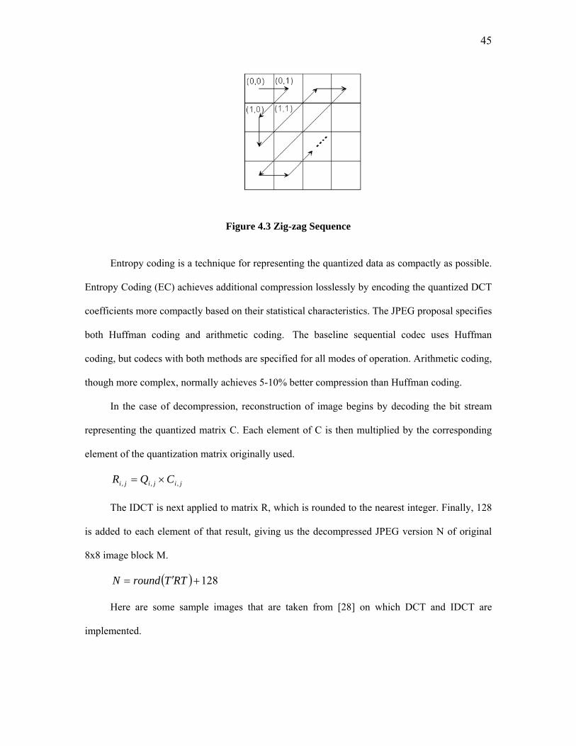
45

Figure 4.3 Zig-zag Sequence

Entropy coding is a technique for representing the quantized data as compactly as possible.

Entropy Coding (EC) achieves additional compression losslessly by encoding the quantized DCT

coefficients more compactly based on their statistical characteristics. The JPEG proposal specifies

both Huffman coding and arithmetic coding. The baseline sequential codec uses Huffman

coding, but codecs with both methods are specified for all modes of operation. Arithmetic coding,

though more complex, normally achieves 5-10% better compression than Huffman coding.

In the case of decompression, reconstruction of image begins by decoding the bit stream

representing the quantized matrix C. Each element of C is then multiplied by the corresponding

element of the quantization matrix originally used.

jijiji CQR ,,, ×=

The IDCT is next applied to matrix R, which is rounded to the nearest integer. Finally, 128

is added to each element of that result, giving us the decompressed JPEG version N of original

8x8 image block M.

( ) 128+′= RTTroundN

Here are some sample images that are taken from [28] on which DCT and IDCT are

implemented.

46

Figure 4.4 Pepper – original image Figure 4.5 DCT of Peppers

Figure 4.6 Quality 20 - 91% Zeros Figure 4.7 Quality 10 – 94% Zeros

4.2. Image Compression Based on Vector Quantization

For compression purpose, a new approach called FTVQ (fast transformed vector

quantization) was proposed, combining together the features of speed improvement, transform

coding and vector quantization. Speed improvement was achieved by fast Kohonen self-

organizing neural network algorithm [31].

Most compression algorithms are either based on transformation first, followed by scalar

quantization and coding; or by direct vector quantization of the original image. Vector

quantization (VQ) is a relatively efficient coding technique used in digital image compression

47

area. The image is partitioned into many blocks, and each block is considered as a vector. Next

figure is used to illustrate this process.

Figure 4.8 Image partitioned into blocks

One important feature of VQ is the possibility of achieving high compression ratios with

relatively small block sizes. Another important advantage of VQ image compression is its fast

decompression by table lookup technique. Neural network approaches have been used for pattern

classification and data clustering. It is possible to apply the training algorithm of neural networks

to the design of appropriate codebook which maximizes the SNR values of reconstructed image.

Kohonen’s self-organizing algorithm classifies inputs into groups that are similar.

Kohonen’s standard approach produced very good results in terms of image quality and level of

compression; however, there is a big disadvantage in terms of long training time.

The basic idea of fast version of the Kohonen’s neural network called FKA (fast Kohonen

algorithm) is choosing winning nodes based on Euclidean distance and weight adjusting based on

input samples are retained.

4.2.1. Fast Transformed Vector Quantization (FTVO)

The approach starts by mapping the original image data into the frequency domain by an

application of a transform such as DCT. Then the produced transformed coefficients are used as

vector components and can be vector quantized. After vector quantizing, the quantizer output are

48

inverse transformed to produce the quantized approximation of the original input image. There is

an advantage that can be obtained by combining transform coding and vector quantization. To

understand how this is possible, it needs to be considered the transform coefficients and their

distribution in the frequency domain. When a linear transform is applied to the original vector

signal, the information is compacted into a subset of the vector components. DCT maps data from

the spatial domain to the frequency domain which often results in that the high energy

components would be concentrated in the low frequency region. This means that the transformed

vector components in the higher frequency regions have very little information.

The low energy components after DCT transform, which account for a certain percentage

of all transformed components, were truncated from each subimage; leaving only the high energy

components. The truncated transformed image was then vector quantized. In our approach, the

vector quantization part is implemented using fast neural network algorithm.

FTVQ is better than VQ in terms of both image quality and training speed. The reason for

this is that the truncated transformed image has less complexity in sample space. Therefore, fewer

output nodes are needed to recover the image than that required by VQ. When we look at images

being compressed, FTVQ result emphasized low frequency information while the overall PSNR

ratio is better than that of VQ. The VQ result has a relatively coarse image, and its fidelity is not

as good as that of FTVQ. Next figure shows an image after standard vector quantization.

Figure 4.9 Quantization

49

4.3. Fractal Image Compression

In fractal image compression the encoding step is computationally expensive. A large

number of sequential searches through a list of domains (portions of the image) are carried out

while trying to find a best match for another image portion [10]. Dietmar proposed that basic

procedure of fractal image compression is equivalent to multi-dimensional nearest neighbor

search. And also, this result is useful for accelerating the encoding procedure in fractal image

compression.

Fractal compression is a lossy compression method introduced by Barnsley and Sloan for

compactly encoding images. The main idea of fractal compression is to exploit local self-

similarity in images. This permits a self-referential description of image data to be yielded. To

find the best matching image portion for each part is known to be the most time consuming part

and numerous strategies have been presented to speed-up encoding. On the other hand, fractal

image compression offers interesting features like fast decoding, independent-resolution and good

image quality at low bit-rates which is useful for off-line applications.

Here, to improve the coding speed, range block and self-similarity domain block are

divided into four classes according to the complexity of blocks: smooth child-block, medium

complicated child-block, simple edge child-block and blend edge child-block. In this method, the

self-similarity of fractal image coding as expanded from 2D to 3D, the error between fractal

collage image and the original image is reduced greatly, Signal-to-Noise Ratio and compressive

ratio are increased greatly, so it is a kind of practical compression method. The coding speed of

fractal coding method based on Notably Irrelevant Check is obviously faster than that of fractal

coding method based on child-block classification, with the PSNR of decoded image has no

distinct decrease. The result is smooth, and there is no obvious square effect, and the compressive

ratio is improved. There are also fast fractal image compression, in which fractal dimension

image segmentation method based on visual characteristic has high compressive ratio, and

50

hierarchy fractal image compression methods. Ugo Erra presented a novel approach to perform

fractal image compression on programmable graphics hardware, which is the first application that

uses the GPU for image compression [11].

Using programmable capabilities of the GPUs, the large amount of inherent parallelism and

memory bandwidth are exploited to perform fast pairing search between portions of the image.

Mapping fractal compression on the GPU happens in this way; in order to exploit the specialized

nature of the GPU and its restricted programming model we must map the fractal compression as

a streaming computation. The goal is to perform pairings test between range and domain

exploiting parallel architecture of the GPU and high bandwidth access to pixels. The entire

process uses a gray level image as input data and returns the textures TPOS with the position of

optimal domain blocks and TSO with scaling/offset coefficients as outputs. Using a

producer/consumer scheme is the main idea of the technique. The producer gathers from the

domain pool a block which is broadcasted to all consumers that are the ranges. Each range stores

the current domain as soon as it appears as the best pairing block. The entire process continues

until all domain blocks have been consumed. In this scenario, a pixel appears as a single floating-

point processor responsible for only one range. Then, the GPU mimics a computational grid

rendering a sized-range rectangular upon which performs parallel pairing test among all the

ranges for a given domain. The results are also pretty satisfactory, the CPU version takes about

280 seconds to perform all pairing test whereas the GPU version takes about 1 second. Then, the

amount of paring test that the GPU is capable to perform is about 64 millions per second whereas

the CPU performs about 220 thousands paring test per second.

Spiral Architecture (SA) is another technique that recently Fractal Compression is used

with [30]. SA is a novel image structure on which images are displayed as a collection of

hexagonal pixels. The selection of range and domain blocks for fractal image compression is

highly related to the uniform image separation specific to SA. It is inspired from anatomical

considerations of the primate’s vision. On Spiral Architecture, an image is a collection of

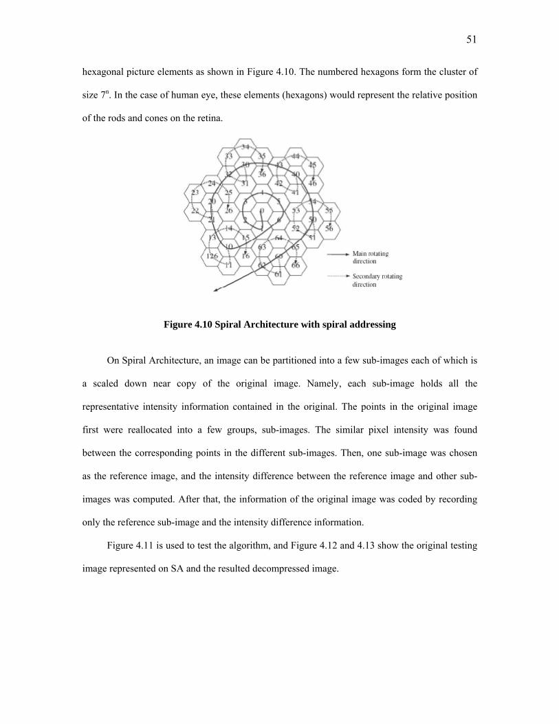
51

hexagonal picture elements as shown in Figure 4.10. The numbered hexagons form the cluster of

size 7n. In the case of human eye, these elements (hexagons) would represent the relative position

of the rods and cones on the retina.

Figure 4.10 Spiral Architecture with spiral addressing

On Spiral Architecture, an image can be partitioned into a few sub-images each of which is

a scaled down near copy of the original image. Namely, each sub-image holds all the

representative intensity information contained in the original. The points in the original image

first were reallocated into a few groups, sub-images. The similar pixel intensity was found

between the corresponding points in the different sub-images. Then, one sub-image was chosen

as the reference image, and the intensity difference between the reference image and other sub-

images was computed. After that, the information of the original image was coded by recording

only the reference sub-image and the intensity difference information.

Figure 4.11 is used to test the algorithm, and Figure 4.12 and 4.13 show the original testing

image represented on SA and the resulted decompressed image.

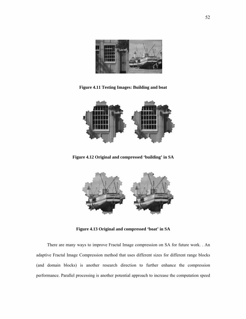
52

Figure 4.11 Testing Images: Building and boat

Figure 4.12 Original and compressed ‘building’ in SA

Figure 4.13 Original and compressed ‘boat’ in SA

There are many ways to improve Fractal Image compression on SA for future work. . An

adaptive Fractal Image Compression method that uses different sizes for different range blocks

(and domain blocks) is another research direction to further enhance the compression

performance. Parallel processing is another potential approach to increase the computation speed

53

and this can be performed through the uniform image separation on SA using a spiral

multiplication [30].

54

CHAPTER 5: IMPLEMENTATION OF DCT ON GPU

5.1. Approach

In this chapter we would like to show how to implement the forward and inverse discrete

cosine transform (DCT) using fragment routines. The DCT can be implemented on 8x8 pixel

blocks which is used as the basis for JPEG compression. Also, 16x16 pixel blocks were tried to

be implemented but because of the limitations of the Cg data types, which supports vectors up to

size of four, the desired results were not satisfactory. The implementation platform was the

GeForce FX 5900 Ultra AGP GPU card, and Cg (C for Graphics) was used as a programming

language.

5.2. Technique

To compress the images, DCT based JPEG image compression technique is used. Most of

the compression techniques, those are implemented till now, are CPU based, however using the

efficient power of GPU, we can make it much faster.

Discrete cosine transform (DCT) is a well-known signal processing tool widely used in

compression standards due to its compact representation power. During compression stage, the

image is divided into NXN blocks,

Figure 5.1 2-D DCT

As you see in the Figure 5.2, 2-D DCT can be obtained by first performing 1-D DCT of the

rows in the matrix, lets name is as X, followed by 1-D DCT of the columns in the calculated

matrix in the first 1-D DCT. After calculating each coefficient according to,

image 1-D DCT 1-D DCT 2-D DCT

55

( ) ( ) ( ) ( )

7,...,1,0,

1612cos

1612cos

22

7

0

7

0,

=

⎟⎠⎞

⎜⎝⎛ +

⎥⎦

⎤⎢⎣

⎡⎟⎠⎞

⎜⎝⎛ +

= ∑ ∑= =

lkwhere

kiljxlckcyi i

ijlkππ

(5.1)

( )⎪⎩

⎪⎨⎧

=1

21

kc otherwisek 0=

( )⎪⎩

⎪⎨⎧

=1

21

lc otherwisel 0=

(5.2)

The compression is achieved by quantizing small value coefficients to zero. Computing

each DCT coefficient according to equations (5.1-5.2) in a block of 8x8 pixels, requires 4096

additions and 4096 multiplications for the whole block. This is too much for a hardware

implementation, even if we use GPU as a processor.

There are several fast methods for computing the DCT. One of them is ANN which is

proposed by Arai, Agui and Nakajima. Arai, Agui and Nakajima showed in 1988 that an 8-point

DCT could be reduced to only 13 multiplications and 27 additions. This version of the DCT,

called ANN, is the fastest one known until now. Figure 5.3 show the flowgraph of the 1-D DCT.

Black dots in the graph represent additions, arrows are multiplications by -1 and boxes are

multiplications.

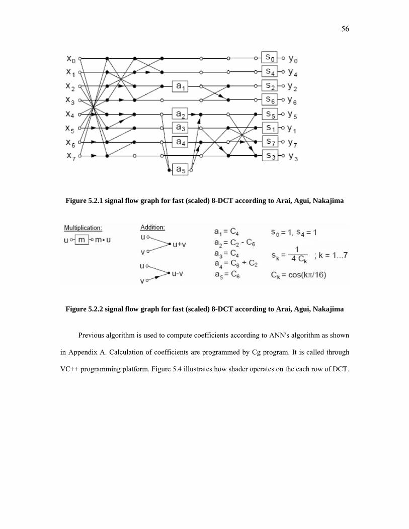
56

Figure 5.2.1 signal flow graph for fast (scaled) 8-DCT according to Arai, Agui, Nakajima

Figure 5.2.2 signal flow graph for fast (scaled) 8-DCT according to Arai, Agui, Nakajima

Previous algorithm is used to compute coefficients according to ANN's algorithm as shown

in Appendix A. Calculation of coefficients are programmed by Cg program. It is called through

VC++ programming platform. Figure 5.4 illustrates how shader operates on the each row of DCT.

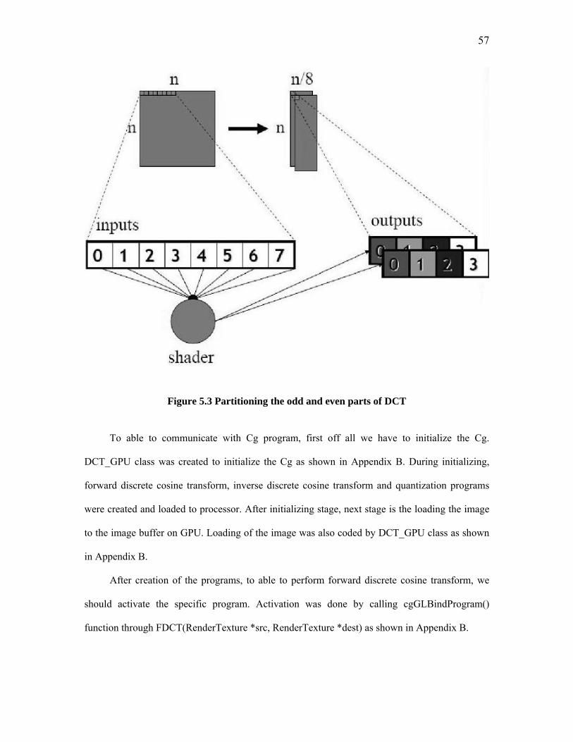
57

Figure 5.3 Partitioning the odd and even parts of DCT

To able to communicate with Cg program, first off all we have to initialize the Cg.

DCT_GPU class was created to initialize the Cg as shown in Appendix B. During initializing,

forward discrete cosine transform, inverse discrete cosine transform and quantization programs

were created and loaded to processor. After initializing stage, next stage is the loading the image

to the image buffer on GPU. Loading of the image was also coded by DCT_GPU class as shown

in Appendix B.

After creation of the programs, to able to perform forward discrete cosine transform, we

should activate the specific program. Activation was done by calling cgGLBindProgram()

function through FDCT(RenderTexture *src, RenderTexture *dest) as shown in Appendix B.

58

Unpacking of the rows and columns follows the forward DCT stage, because we need to

rearrange data into correct order. When it comes to partition the DCT, Render shader gets the

1/8th of the width or height and returns the corrected data. Then shader reads 8 neighboring texels,

and writes outputs to RGBA components of two render target using MRT.

After FDCT is done, next stage is the quantization. Default quantization level is defined as

2.0. Here, again as we did during FDCT, we called the Quantize(RenderTexture *src,

RenderTexture *dest, float quantize_level) function through DCT_GPU class as shown in

Appendix B. Quantize function activated the quantized program which was already created

during initializing of the Cg.

After Quantization is done now data should be unpacked on subsequent passes during the

process of IDCT. Again 2-D IDCT can be done by 1-D IDCT on each column followed by 1-D

IDCT on each row. To calculate quantized coefficients again AAN method is used. The inverse

ANN is obtained from the right to left in the flowgraph in Figure 5.3. During IDCT, again rows

and columns were divided into two passes as done during DCT. This process also implemented

by using Cg as shown in Appendix C. And at last, we unpacked the columns and rows to convert

greyscale image packed into 2 RGBA textures into a single image 8 times as wide.

59

CHAPTER 6: RESULTS

By defining glutInitWindowSize (512,512), at the same time we also define the limits of

the pixels that we are going to compress. If we want to compress an image bigger than 512x512,

we should change this command line to this,

glutInitWindowSize(1024, 1024);

or;

glutInitWindowSize(2048, 2048).

Program was tested on nine pictures, with sizes from 90Kb to 300Kb. Other then child.png

image all of the other images were 512x512 pixel size, child.png is 256x256 pixel size.

Unfortunately, program supports only the “png” type images for now.

Figure 5.5 shows the command window;

60

Figure 5.4 Program View

And next figure shows a demonstration of the program;

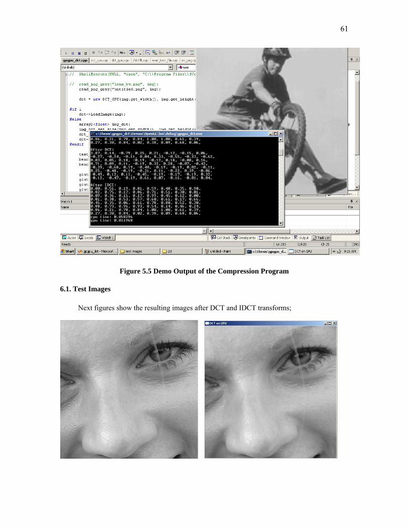
61

Figure 5.5 Demo Output of the Compression Program

6.1. Test Images

Next figures show the resulting images after DCT and IDCT transforms;

62

Figure 5.14 eye.png Figure 5.15 After IDCT

Figure 5.14 Comic.png Figure 5.15 After IDCT

Figure 5.14 Child.png Figure 5.15 After IDCT

63

Figure 5.13 Original Image – serpil2.png

64

Figure 5.14 After DCT Figure 5.15 After IDCT

Figure 5.16 Original Image – serpil3.png

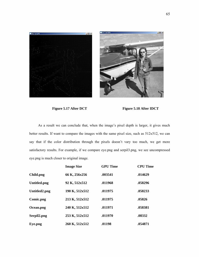
65

Figure 5.17 After DCT Figure 5.18 After IDCT

As a result we can conclude that, when the image’s pixel depth is larger, it gives much

better results. If want to compare the images with the same pixel size, such as 512x512, we can

say that if the color distribution through the pixels doesn’t vary too much, we get more

satisfactory results. For example, if we compare eye.png and serpil3.png, we see uncompressed

eye.png is much closer to original image.

Image Size GPU Time CPU Time

Child.png 66 K, 256x256 .003541 .014629

Untitled.png 92 K, 512x512 .011968 .058296

Untitled2.png 190 K, 512x512 .011975 .058233

Comic.png 213 K, 512x512 .011975 .05826

Ocean.png 240 K, 512x512 .011971 .058381

Serpil2.png 253 K, 512x512 .011970 .08332

Eye.png 260 K, 512x512 .01198 .054871

66

Serpil3.png 275 K, 512x512 .01197 .05833

Untitled1.png 308 K, 512x512 .01198 .058326

Table 6.1 Time consuming of the GPU and CPU usage over the whole program

DCT Performance

00.010.020.030.040.050.060.070.080.09

66 K, 2

56x2

56

92 K, 5

12x5

12

190 K

, 512

x512

213 K

, 512

x512

240 K

, 512

x512

253 K

, 512

x512

260 K

, 512

x512

275 K

, 512

x512

308 K

, 512

x512

Size (Kb)

Tim

e (s

n)

GPU TimeCPU Time

Chart 6.1 Proportional Time consumed according to size of an image

As we can see from the chart and table also, when size of the image increases CPU time

also increases. On the other hand, increment of the size doesn’t affect the GPU timing, because it

is already so small. As we can see even uploading of the image takes more time then the whole

GPU process, so implementing the image compression on GPU is a great achievement for saving

of processing time.

67

CHAPTER 7: CONCLUSION

By this thesis we explored the processing power of GPUs for digital image compression

using discrete cosine transform. Experimental results showed that GPU gave almost five times

faster results than CPU did. We used Cg programming language as a shader language, and used

VC++ 7.1 as an interface between user and the GPU. Cg program was called by a C++ function.

At the sight of experimental results we became sure that GPU’s efficient processing power

and algorithms are good fit for implementing Digital Image Processing Standards. For making the

program even more efficient ANN algorithm is used to calculate the coefficients of the DCT

compression. And using the shaders at the stage of partitioning of the DCT blocks with Cg

programming language helped us at saving the most of the processing time. But it is still not

perfect, because Cg has its own limitations also, it is not developed for general purpose

programming completely. If we want to compress the image with 16x16 blocks, since Cg doesn’t

let us to use vector of size 8, it would be much more complicated.

If we can also do color space conversion by using GPU, it would be very helpful, because

right now user has to convert the image to grayscale outside the program by using another

application. First I though about calling some Matlab functions for color space conversion from

C++ files, but when I install the Cg and the Matlab together at the same Pc, somehow system just

confuses up and Mablab doesn’t let Cg to do its part.

Another limitation with this program is that it can only compress *.png files, at future

applications if we can expand the type of the input image, it can be more useful. Because not

everybody wants to work with only png files.

68

Reference:

[1-37] 1. Aaron Lefohn, I.B., Patrick McCormick,John Owens, Timothy Purcell, Robert

Strzodka, General Purpose Computation on Graphics Hardware, in GPGPU,

www.gpgpu.org, Editor. 2005.

2. Aaron Lefohn, J.M.K., Robert Strzodka, Shubhabrata Sengupta, John D. Owens

Glift: Generic, Efficient, Randon-Access GPU Data Structures. ACM

Transactions on Graphics, 2006. 25: p. 1-37.

3. Andreas Griesser, S.D.R., Alexander Neubeck, Luc Van Gool, GPU-Based

Foreground-Background Segmentation using an Extended Colinearity Criterion.

VMV 2005, 2005: p. 319-326.

4. Bjorke, K., Introduction to Image Processing on the GPU. 2005, NVIDIA.

5. Bo Fang, G.S., Shipeng Li, Huifang Chen, Techniques for efficient DCT/IDCT

implementation on generic GPU. IEEE International Symposium, 2005. 2: p.

1126-1129.

6. Bryson R. Payne, S.O.B., G. Scott Owen, Michael C. Weeks, Ying Zhu (2005)

Accelerated 2D Image Processing on GPUs. Computational Science – ICCS

2005: 5th International Conference, Atlanta, GA, USA, May 22-25, 2005.

Proceedings, Part II Volume, 256

7. Chris J. Thompson, S.H., Mark Oskin, Using Modern Graphics Architectures for

General-Purpose Computing: A Framework and Analysis. Annual IEEE/ACM

International Symposium on Microarchitecture (MICRO-35), 2002: p. 306.

69

8. developer.nvidia.com. Cg - Teaching Cg. Teaching with The Cg Tutorial [cited;

Presentation]. Available from:

http://developer.nvidia.com/object/cg_tutorial_teaching.html.

9. E. Scott Larsen, D.M., Fast matrix multiplies using graphics hardware. ACM

Press, 2001: p. 55-60.

10. Erjun Zhao, D.L., Fractal Image Compression Methods: A Review. IEEE, 2005.

11. Erra, U., Toward Real Time Fractal Image Compression Using Graphics

Hardware. Springer - Verlag, 2005. 3804: p. 723-728.

12. Gent, K.C.a.P., Image Compression and the Discrete Cosine Transform. 1998,

College of the Redwoods.

13. Geoffrey M. Davis, A.N., Wavelet-based Image Coding: An Overview. Applied

and Computational Control, Signals, and Circuits, 1998. 1.

14. Green, S. Image Processing Tricks in OpenGL. in GameDevelopers Conference.

2005. San Francisco: NVIDIA Corporation.

15. Griesser, A., Real-Time, GPU-based Foreground-Backgroung Segmentation.

2005, Swiss Federal Institute of Technology: Zurich.

16. IkkJin Ahn, M.L., Paul Turner, Image Processing on the GPU. 2005.

17. Jargstorff, F., GPU Image Processing, in SIGGRAPH 2004. 2004, NVIDIA.

18. John D Owens, D.L., Naga Govindaraju, Mark Harris, Jen Kruger, Aaron E.

Lefohn, and Timothy J. Purcell, A Survey of General-Purpose Computation on

Graphics Hardware. EUROGRAPHICS 2005, 2005.

70

19. John D. Owens, D.L., Naga Govindaraju, Mark Harris, Jens Kruger, Aoron E.

Lefohn, Timothy J. Purcell, A Survey of General-Purpose Computation on

Graphics Hardware. EUROGRAPHICS 2005, 2005.

20. Kenneth Moreland, E.A., Simulation and computation: The FFT on a GPU ACM

PORTAL, 2003: p. 112-119.

21. M. Rumpf, R.S., Nonlinear Diffusion in Graphics Hardware. EG/IEEE TCVG

Symposium on Visualization VisSym, 2001: p. 75-84.

22. Michael F. Barnsley, A.D.S., A Better Way to Compress Images, in BYTE. 1988.

p. 215-223.

23. Ming Yang, N.B., An Overview of Lossless Digital Image Compression

Techniques. IEEE, 2005.

24. Nicola Candussi, S.D., Tobias Hollerer Real-time Rendering with Wavelet-

Compressed Multi-Dimensional Textures on the GPU. 2005, University of

California: California.

25. Nolan Goodnight, R.W., Greg Humphreys, Computation on Programmable

Graphics Hardware. IEEE Computer Society, 2005. 25: p. 12-15.

26. NVIDIA, Cg Language Specification, NVIDIA, Editor. 2005, NVIDIA.

27. Owens, J. The GPGPU Programming Model. 2005 2005 [cited 2005; Available

from: http://www.gpgpu.org/vis2005/PDFs/C.owens.mapping.pdf.

28. P. Moravie, H.E., C. Lambert-Nebout, J.-L Basille, Real-time image compression

using SIMD architectures. IEEE, 1995: p. 274-279.

29. Peter L. Venetianer, T.R., Image Compression by Cellular Neural Networks.

IEEE Transactions on Cirsuits and Systems, 1998. 45(3): p. 205-215.

71

30. Philippe Colantoni, N.B., Jerome Da Rugna, Fast and Accurate Color Image

Processing Using 3D Graphics Cards. VMV, 2003.

31. Rafael C. Gonzalez, R.E.W., Digital Image Processing, ed. n. Edition. 2002:

Printice-Hall Inc.

32. Robert Li, J.K., Image Compression Using Fast Transformed Vector

Quantization. IEEE, 2000: p. 141-145.

33. Ruigang Yang, G.W., Fast Image Segmentation and Smoothing Using Commodity

Graphics Hardware. Journal of Graphics Tools, 2002. 7(4).

34. Saha, S., Image Compression - from DCT to Wavelets: A Review, in The ACM

Student Magazine. 2000.

35. Schouten, T., Chapter 6 Image Compression, in Course RT2: Image Processing.

2006.

36. Strzodka, R., Advanced Image Processing, in GPGPU, I. VIS, Editor. 2005,

www.gpgpu.org.

37. Xiangjian He, H.W., Qiang Qu, Tom Hintz and Namho Hur, Fractal Image

Compression on Spiral Architecture. IEEE, CGIV'06, 2006.

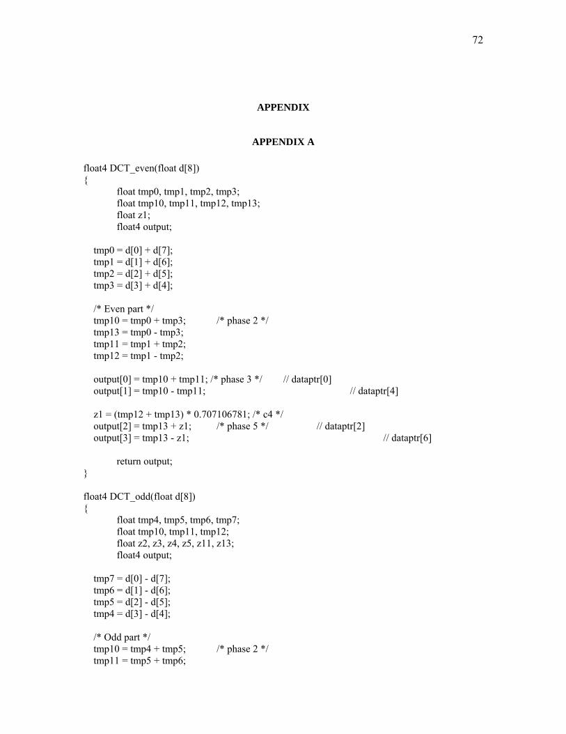
72

APPENDIX

APPENDIX A

float4 DCT_even(float d[8]) { float tmp0, tmp1, tmp2, tmp3; float tmp10, tmp11, tmp12, tmp13; float z1; float4 output; tmp0 = d[0] + d[7]; tmp1 = d[1] + d[6]; tmp2 = d[2] + d[5]; tmp3 = d[3] + d[4]; /* Even part */ tmp10 = tmp0 + tmp3; /* phase 2 */ tmp13 = tmp0 - tmp3; tmp11 = tmp1 + tmp2; tmp12 = tmp1 - tmp2; output[0] = tmp10 + tmp11; /* phase 3 */ // dataptr[0] output[1] = tmp10 - tmp11; // dataptr[4] z1 = (tmp12 + tmp13) * 0.707106781; /* c4 */ output[2] = tmp13 + z1; /* phase 5 */ // dataptr[2] output[3] = tmp13 - z1; // dataptr[6] return output; } float4 DCT_odd(float d[8]) { float tmp4, tmp5, tmp6, tmp7; float tmp10, tmp11, tmp12; float z2, z3, z4, z5, z11, z13; float4 output; tmp7 = d[0] - d[7]; tmp6 = d[1] - d[6]; tmp5 = d[2] - d[5]; tmp4 = d[3] - d[4]; /* Odd part */ tmp10 = tmp4 + tmp5; /* phase 2 */ tmp11 = tmp5 + tmp6;

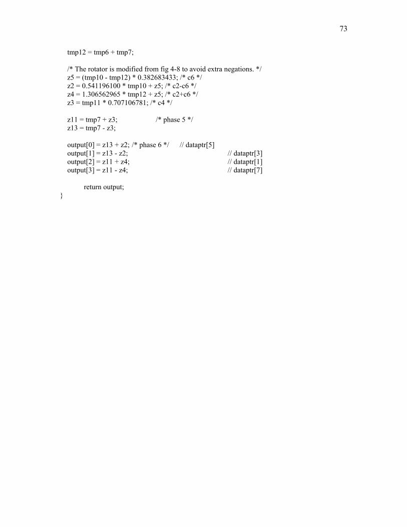
73

tmp12 = tmp6 + tmp7; /* The rotator is modified from fig 4-8 to avoid extra negations. */ z5 = (tmp10 - tmp12) * 0.382683433; /* c6 */ z2 = 0.541196100 * tmp10 + z5; /* c2-c6 */ z4 = 1.306562965 * tmp12 + z5; /* c2+c6 */ z3 = tmp11 * 0.707106781; /* c4 */ z11 = tmp7 + z3; /* phase 5 */ z13 = tmp7 - z3; output[0] = z13 + z2; /* phase 6 */ // dataptr[5] output[1] = z13 - z2; // dataptr[3] output[2] = z11 + z4; // dataptr[1] output[3] = z11 - z4; // dataptr[7] return output; }

74

APPENDIX B

DCT_GPU::DCT_GPU(int w, int h, bool use_mrt) : width(w), height(h), mrt(use_mrt) { char *format = "float=16 rgba textureRECT"; // char *format = "float=32 rgba textureRECT"; // create buffers img_buffer = CreateBuffer(w, h, format); dest_buffer = CreateBuffer(w, h, format); temp_buffer = CreateBuffer(w, h, format); row_buffer = CreateBuffer(w/8, h, format); if (!mrt) row_buffer2 = CreateBuffer(w/8, h, format); col_buffer = CreateBuffer(w, h/8, format); if (!mrt) col_buffer2 = CreateBuffer(w, h/8, format); InitCg(); } void DCT_GPU::InitCg() { cgSetErrorCallback(cgErrorCallback); g_context = cgCreateContext(); const char *code = read_text_file("gpgpu_dct/dct.cg"); fprog_profile = cgGLGetLatestProfile(CG_GL_FRAGMENT); if (mrt) { dct_rows_fprog = cgCreateProgram(g_context, CG_SOURCE, code, fprog_profile, "DCT_rows_singlepass_PS", NULL); } else { dct_rows_fprog = cgCreateProgram(g_context, CG_SOURCE, code, fprog_profile, "DCT_rows_pass1_PS", NULL); dct_rows2_fprog = cgCreateProgram(g_context, CG_SOURCE, code, fprog_profile, "DCT_rows_pass2_PS", NULL); } dct_unpack_rows_fprog = cgCreateProgram(g_context, CG_SOURCE, code, fprog_profile, "DCT_unpack_rows_PS", NULL); if (mrt) { dct_cols_fprog = cgCreateProgram(g_context, CG_SOURCE, code, fprog_profile, "DCT_cols_singlepass_PS", NULL); } else { dct_cols_fprog = cgCreateProgram(g_context, CG_SOURCE, code, fprog_profile, "DCT_cols_pass1_PS", NULL);

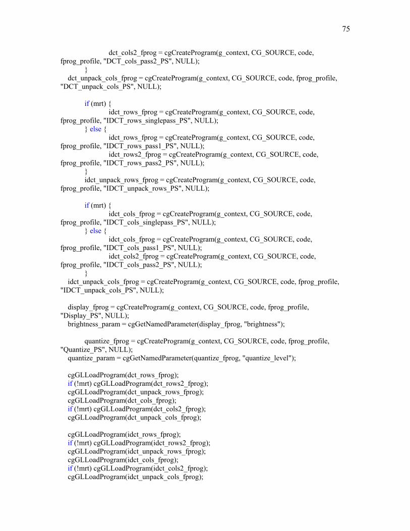
75

dct_cols2_fprog = cgCreateProgram(g_context, CG_SOURCE, code, fprog_profile, "DCT_cols_pass2_PS", NULL); } dct_unpack_cols_fprog = cgCreateProgram(g_context, CG_SOURCE, code, fprog_profile, "DCT_unpack_cols_PS", NULL); if (mrt) { idct_rows_fprog = cgCreateProgram(g_context, CG_SOURCE, code, fprog_profile, "IDCT_rows_singlepass_PS", NULL); } else { idct_rows_fprog = cgCreateProgram(g_context, CG_SOURCE, code, fprog_profile, "IDCT_rows_pass1_PS", NULL); idct_rows2_fprog = cgCreateProgram(g_context, CG_SOURCE, code, fprog_profile, "IDCT_rows_pass2_PS", NULL); } idct_unpack_rows_fprog = cgCreateProgram(g_context, CG_SOURCE, code, fprog_profile, "IDCT_unpack_rows_PS", NULL); if (mrt) { idct_cols_fprog = cgCreateProgram(g_context, CG_SOURCE, code, fprog_profile, "IDCT_cols_singlepass_PS", NULL); } else { idct_cols_fprog = cgCreateProgram(g_context, CG_SOURCE, code, fprog_profile, "IDCT_cols_pass1_PS", NULL); idct_cols2_fprog = cgCreateProgram(g_context, CG_SOURCE, code, fprog_profile, "IDCT_cols_pass2_PS", NULL); } idct_unpack_cols_fprog = cgCreateProgram(g_context, CG_SOURCE, code, fprog_profile, "IDCT_unpack_cols_PS", NULL); display_fprog = cgCreateProgram(g_context, CG_SOURCE, code, fprog_profile, "Display_PS", NULL); brightness_param = cgGetNamedParameter(display_fprog, "brightness"); quantize_fprog = cgCreateProgram(g_context, CG_SOURCE, code, fprog_profile, "Quantize_PS", NULL); quantize_param = cgGetNamedParameter(quantize_fprog, "quantize_level"); cgGLLoadProgram(dct_rows_fprog); if (!mrt) cgGLLoadProgram(dct_rows2_fprog); cgGLLoadProgram(dct_unpack_rows_fprog); cgGLLoadProgram(dct_cols_fprog); if (!mrt) cgGLLoadProgram(dct_cols2_fprog); cgGLLoadProgram(dct_unpack_cols_fprog); cgGLLoadProgram(idct_rows_fprog); if (!mrt) cgGLLoadProgram(idct_rows2_fprog); cgGLLoadProgram(idct_unpack_rows_fprog); cgGLLoadProgram(idct_cols_fprog); if (!mrt) cgGLLoadProgram(idct_cols2_fprog); cgGLLoadProgram(idct_unpack_cols_fprog);

76

cgGLLoadProgram(display_fprog); cgGLLoadProgram(quantize_fprog); delete [] code; }

void DCT_GPU::LoadImage(array2<unsigned char> &img) { glGenTextures(1, &img_tex); glBindTexture(GL_TEXTURE_RECTANGLE_NV, img_tex); glTexParameteri(GL_TEXTURE_RECTANGLE_NV, GL_TEXTURE_WRAP_S, GL_CLAMP_TO_EDGE); glTexParameteri(GL_TEXTURE_RECTANGLE_NV, GL_TEXTURE_WRAP_T, GL_CLAMP_TO_EDGE); glTexParameteri(GL_TEXTURE_RECTANGLE_NV, GL_TEXTURE_MAG_FILTER, GL_NEAREST); glTexParameteri(GL_TEXTURE_RECTANGLE_NV, GL_TEXTURE_MIN_FILTER, GL_NEAREST); glTexImage2D(GL_TEXTURE_RECTANGLE_NV, 0, GL_LUMINANCE, img.get_width(), img.get_height(), 0, GL_LUMINANCE, GL_UNSIGNED_BYTE, (const void *)img.get_pointer()); img_buffer->Activate(); DisplayTexture(img_tex); img_buffer->Deactivate(); }

void DCT_GPU::FDCT(RenderTexture *src, RenderTexture *dest) { if (mrt) { Pass_MRT(dct_rows_fprog, src, WGL_FRONT_LEFT_ARB, 0, row_buffer, GL_AUX0, GL_AUX1); Pass_MRT(dct_unpack_rows_fprog, row_buffer, WGL_AUX0_ARB, WGL_AUX1_ARB, dest, GL_FRONT_LEFT, 0); Pass_MRT(dct_cols_fprog, dest, WGL_FRONT_LEFT_ARB, 0, col_buffer, GL_AUX0, GL_AUX1); Pass_MRT(dct_unpack_cols_fprog, col_buffer, WGL_AUX0_ARB, WGL_AUX1_ARB, dest, GL_FRONT_LEFT, 0); } else { Pass(dct_rows_fprog, src, 0, row_buffer); Pass(dct_rows2_fprog, src, 0, row_buffer2); Pass(dct_unpack_rows_fprog, row_buffer, row_buffer2, dest); Pass(dct_cols_fprog, dest, 0, col_buffer); Pass(dct_cols2_fprog, dest, 0, col_buffer2); Pass(dct_unpack_cols_fprog, col_buffer, col_buffer2, dest); }

77

}

void DCT_GPU::Quantize(RenderTexture *src, RenderTexture *dest, float quantize_level) { cgGLSetParameter1f(quantize_param, quantize_level); Pass(quantize_fprog, src, 0, dest); }

78

APPENDIX C

float4 IDCT_1(float d[8]) { float tmp0, tmp1, tmp2, tmp3, tmp4, tmp5, tmp6, tmp7; float tmp10, tmp11, tmp12, tmp13; float z5, z10, z11, z12, z13; float4 output; /* Even part */ tmp0 = d[0]; tmp1 = d[2]; tmp2 = d[4]; tmp3 = d[6]; tmp10 = tmp0 + tmp2; /* phase 3 */ tmp11 = tmp0 - tmp2; tmp13 = tmp1 + tmp3; /* phases 5-3 */ tmp12 = (tmp1 - tmp3) * 1.414213562 - tmp13; /* 2*c4 */ tmp0 = tmp10 + tmp13; /* phase 2 */ tmp3 = tmp10 - tmp13; tmp1 = tmp11 + tmp12; tmp2 = tmp11 - tmp12; /* Odd part */ tmp4 = d[1]; tmp5 = d[3]; tmp6 = d[5]; tmp7 = d[7]; z13 = tmp6 + tmp5; /* phase 6 */ z10 = tmp6 - tmp5; z11 = tmp4 + tmp7; z12 = tmp4 - tmp7; tmp7 = z11 + z13; /* phase 5 */ tmp11 = (z11 - z13) * 1.414213562; /* 2*c4 */ z5 = (z10 + z12) * 1.847759065; /* 2*c2 */ tmp10 = 1.082392200 * z12 - z5; /* 2*(c2-c6) */ tmp12 = -2.613125930 * z10 + z5; /* -2*(c2+c6) */ tmp6 = tmp12 - tmp7; /* phase 2 */ tmp5 = tmp11 - tmp6; tmp4 = tmp10 + tmp5;

79

output[0] = tmp0 + tmp7; // wsptr[DCTSIZE*0] // output[7] = tmp0 - tmp7; // wsptr[DCTSIZE*7] output[1] = tmp1 + tmp6; // wsptr[DCTSIZE*1] // output[6] = tmp1 - tmp6; // wsptr[DCTSIZE*6] output[2] = tmp2 + tmp5; // wsptr[DCTSIZE*2] // output[5] = tmp2 - tmp5; // wsptr[DCTSIZE*5] // output[4] = tmp3 + tmp4; // wsptr[DCTSIZE*4] output[3] = tmp3 - tmp4; // wsptr[DCTSIZE*3] return output; } float4 IDCT_2(float d[8]) { float tmp0, tmp1, tmp2, tmp3, tmp4, tmp5, tmp6, tmp7; float tmp10, tmp11, tmp12, tmp13; float z5, z10, z11, z12, z13; float4 output; /* Even part */ tmp0 = d[0]; tmp1 = d[2]; tmp2 = d[4]; tmp3 = d[6]; tmp10 = tmp0 + tmp2; /* phase 3 */ tmp11 = tmp0 - tmp2; tmp13 = tmp1 + tmp3; /* phases 5-3 */ tmp12 = (tmp1 - tmp3) * 1.414213562 - tmp13; /* 2*c4 */ tmp0 = tmp10 + tmp13; /* phase 2 */ tmp3 = tmp10 - tmp13; tmp1 = tmp11 + tmp12; tmp2 = tmp11 - tmp12; /* Odd part */ tmp4 = d[1]; tmp5 = d[3]; tmp6 = d[5]; tmp7 = d[7]; z13 = tmp6 + tmp5; /* phase 6 */ z10 = tmp6 - tmp5; z11 = tmp4 + tmp7; z12 = tmp4 - tmp7; tmp7 = z11 + z13; /* phase 5 */ tmp11 = (z11 - z13) * 1.414213562; /* 2*c4 */ z5 = (z10 + z12) * 1.847759065; /* 2*c2 */ tmp10 = 1.082392200 * z12 - z5; /* 2*(c2-c6) */

80

tmp12 = -2.613125930 * z10 + z5; /* -2*(c2+c6) */ tmp6 = tmp12 - tmp7; /* phase 2 */ tmp5 = tmp11 - tmp6; tmp4 = tmp10 + tmp5; // output[0] = tmp0 + tmp7; // wsptr[DCTSIZE*0] output[3] = tmp0 - tmp7; // wsptr[DCTSIZE*7] // output[1] = tmp1 + tmp6; // wsptr[DCTSIZE*1] output[2] = tmp1 - tmp6; // wsptr[DCTSIZE*6] // output[2] = tmp2 + tmp5; // wsptr[DCTSIZE*2] output[1] = tmp2 - tmp5; // wsptr[DCTSIZE*5] output[0] = tmp3 + tmp4; // wsptr[DCTSIZE*4] // output[3] = tmp3 - tmp4; // wsptr[DCTSIZE*3] return output; }