DCT based SPIHT architecture for hyperspectral …cj82ps144/...DCT Based SPIHT Architecture for...
77
DCT Based SPIHT Architecture for Hyperspectral Image Data Compression A Thesis Presented by Jieming Xu to The Department of Electrical and Computer Engineering in partial fulfillment of the requirements for the degree of Master of Science in Electrical and Computer Engineering Northeastern University Boston, Massachusetts August 2016
Transcript of DCT based SPIHT architecture for hyperspectral …cj82ps144/...DCT Based SPIHT Architecture for...
DCT Based SPIHT Architecture for Hyperspectral Image Data
Compression
A Thesis Presented
by
Jieming Xu
to
The Department of Electrical and Computer Engineering
in partial fulfillment of the requirements
for the degree of
Master of Science
in
Electrical and Computer Engineering
Northeastern University
Boston, Massachusetts
August 2016
Contents
List of Figures iii
List of Tables v
List of Acronyms vi
Acknowledgments vii
Abstract of the Thesis viii
1 Introduction 11.1 Hyperspectal image . . . . . . . . . . . . . . . . . . . . . . . . . . . . . . . . . . 1
1.1.1 AVIRIS Data . . . . . . . . . . . . . . . . . . . . . . . . . . . . . . . . . 21.1.2 AIRS Data . . . . . . . . . . . . . . . . . . . . . . . . . . . . . . . . . . 31.1.3 Reflection Bands . . . . . . . . . . . . . . . . . . . . . . . . . . . . . . . 31.1.4 Radiation Models . . . . . . . . . . . . . . . . . . . . . . . . . . . . . . . 3
1.2 Hyperspectral Image Data Compression . . . . . . . . . . . . . . . . . . . . . . . 61.2.1 Lossy & Lossless Compression . . . . . . . . . . . . . . . . . . . . . . . 61.2.2 Distortion Measure . . . . . . . . . . . . . . . . . . . . . . . . . . . . . . 71.2.3 Rate-Distortion Curve . . . . . . . . . . . . . . . . . . . . . . . . . . . . 91.2.4 Spectral & Spatial Accessibility . . . . . . . . . . . . . . . . . . . . . . . 101.2.5 Hyperspectral Compression System . . . . . . . . . . . . . . . . . . . . . 10
1.3 Summary . . . . . . . . . . . . . . . . . . . . . . . . . . . . . . . . . . . . . . . 11
2 Review of Background in Signal Coding 122.1 Coding Techniques . . . . . . . . . . . . . . . . . . . . . . . . . . . . . . . . . . 12
2.1.1 Entropy Coding . . . . . . . . . . . . . . . . . . . . . . . . . . . . . . . . 122.1.2 Linear-Predictive Coding . . . . . . . . . . . . . . . . . . . . . . . . . . . 132.1.3 Vector Quantization . . . . . . . . . . . . . . . . . . . . . . . . . . . . . 142.1.4 Bitplane Coding . . . . . . . . . . . . . . . . . . . . . . . . . . . . . . . 15
2.2 Transform Coding . . . . . . . . . . . . . . . . . . . . . . . . . . . . . . . . . . . 162.2.1 Discrete Cosine Transform . . . . . . . . . . . . . . . . . . . . . . . . . . 162.2.2 Discrete Wavelet Transform . . . . . . . . . . . . . . . . . . . . . . . . . 172.2.3 KL Transform . . . . . . . . . . . . . . . . . . . . . . . . . . . . . . . . 19
i
2.3 Wavelet-based Coding techniques . . . . . . . . . . . . . . . . . . . . . . . . . . 192.3.1 Embedded Zerotree Wavelet (EZW) . . . . . . . . . . . . . . . . . . . . . 202.3.2 Wavelet Difference Reduction (WDR) . . . . . . . . . . . . . . . . . . . . 212.3.3 Set Partitioning In Hierarchical Trees (SPIHT) . . . . . . . . . . . . . . . 212.3.4 EBCOT & JPEG2000 . . . . . . . . . . . . . . . . . . . . . . . . . . . . 23
2.4 Proposed Algorithm . . . . . . . . . . . . . . . . . . . . . . . . . . . . . . . . . . 242.5 Summary . . . . . . . . . . . . . . . . . . . . . . . . . . . . . . . . . . . . . . . 24
3 Architecture Details 253.1 3D-SPIHT . . . . . . . . . . . . . . . . . . . . . . . . . . . . . . . . . . . . . . . 25
3.1.1 Code-Block Introduction . . . . . . . . . . . . . . . . . . . . . . . . . . . 253.1.2 Algorithm . . . . . . . . . . . . . . . . . . . . . . . . . . . . . . . . . . . 27
3.2 SPIHT Performance Evaluation . . . . . . . . . . . . . . . . . . . . . . . . . . . . 293.3 Cube Transformation & Organization . . . . . . . . . . . . . . . . . . . . . . . . 33
3.3.1 3D-DCT . . . . . . . . . . . . . . . . . . . . . . . . . . . . . . . . . . . 333.3.2 3D-DWT . . . . . . . . . . . . . . . . . . . . . . . . . . . . . . . . . . . 333.3.3 DWT Cube Organization . . . . . . . . . . . . . . . . . . . . . . . . . . . 353.3.4 DCT Cube Organization . . . . . . . . . . . . . . . . . . . . . . . . . . . 36
3.4 Level Shifting . . . . . . . . . . . . . . . . . . . . . . . . . . . . . . . . . . . . . 363.5 Summary . . . . . . . . . . . . . . . . . . . . . . . . . . . . . . . . . . . . . . . 38
4 Practical Implementations 414.1 Compression System . . . . . . . . . . . . . . . . . . . . . . . . . . . . . . . . . 414.2 Post Compression Rate Distortion (PCRD) Algorithm . . . . . . . . . . . . . . . . 444.3 PCRD Algorithm Optimization . . . . . . . . . . . . . . . . . . . . . . . . . . . . 464.4 Parallel Computing . . . . . . . . . . . . . . . . . . . . . . . . . . . . . . . . . . 484.5 Summary . . . . . . . . . . . . . . . . . . . . . . . . . . . . . . . . . . . . . . . 50
5 Results & Analysis 525.1 Compression Results . . . . . . . . . . . . . . . . . . . . . . . . . . . . . . . . . 52
5.1.1 Results in SNR . . . . . . . . . . . . . . . . . . . . . . . . . . . . . . . . 535.1.2 Results in Spectral Profile . . . . . . . . . . . . . . . . . . . . . . . . . . 53
5.2 Analysis . . . . . . . . . . . . . . . . . . . . . . . . . . . . . . . . . . . . . . . . 565.3 Summary . . . . . . . . . . . . . . . . . . . . . . . . . . . . . . . . . . . . . . . 58
6 Conclusions and Future Work 616.1 Conclusion . . . . . . . . . . . . . . . . . . . . . . . . . . . . . . . . . . . . . . 616.2 Future Work . . . . . . . . . . . . . . . . . . . . . . . . . . . . . . . . . . . . . . 62
Bibliography 63
A SPIHT Recursive Functions 65A.1 Encoding Cost in Best Case . . . . . . . . . . . . . . . . . . . . . . . . . . . . . . 65A.2 Encoding Cost in Case A . . . . . . . . . . . . . . . . . . . . . . . . . . . . . . . 65A.3 Encoding Cost in Case B & Case C . . . . . . . . . . . . . . . . . . . . . . . . . . 66
ii
List of Figures
1.1 Hyperspectral Image Structure . . . . . . . . . . . . . . . . . . . . . . . . . . . . 21.2 Solar Radiation Model . . . . . . . . . . . . . . . . . . . . . . . . . . . . . . . . 41.3 Spectral Signature of Different Objects . . . . . . . . . . . . . . . . . . . . . . . . 51.4 Atmosphere Transmittance . . . . . . . . . . . . . . . . . . . . . . . . . . . . . . 61.5 Object Reflectance Curve . . . . . . . . . . . . . . . . . . . . . . . . . . . . . . . 71.6 Rate-Distortion Curve . . . . . . . . . . . . . . . . . . . . . . . . . . . . . . . . . 91.7 Transmitter . . . . . . . . . . . . . . . . . . . . . . . . . . . . . . . . . . . . . . 101.8 Receiver . . . . . . . . . . . . . . . . . . . . . . . . . . . . . . . . . . . . . . . . 10
2.1 Predictive Coding System . . . . . . . . . . . . . . . . . . . . . . . . . . . . . . . 142.2 Multi-level Decomposition . . . . . . . . . . . . . . . . . . . . . . . . . . . . . . 182.3 Harr Wavelets . . . . . . . . . . . . . . . . . . . . . . . . . . . . . . . . . . . . . 182.4 2-Level Wavelet Decomposition . . . . . . . . . . . . . . . . . . . . . . . . . . . 202.5 8×8 Block Coefficients and MSB Map . . . . . . . . . . . . . . . . . . . . . . . 22
3.1 3 Dimensional DWT . . . . . . . . . . . . . . . . . . . . . . . . . . . . . . . . . 263.2 3D-Hierarchical Tree Organization . . . . . . . . . . . . . . . . . . . . . . . . . . 273.3 Set patronization in DWT . . . . . . . . . . . . . . . . . . . . . . . . . . . . . . . 303.4 2-Level Filter Bank . . . . . . . . . . . . . . . . . . . . . . . . . . . . . . . . . . 343.5 Implementation of 3D-DWT . . . . . . . . . . . . . . . . . . . . . . . . . . . . . 343.6 3D Filter Bank . . . . . . . . . . . . . . . . . . . . . . . . . . . . . . . . . . . . 353.7 Cube Tiling . . . . . . . . . . . . . . . . . . . . . . . . . . . . . . . . . . . . . . 363.8 Level Shifting Comparasion . . . . . . . . . . . . . . . . . . . . . . . . . . . . . 37
4.1 Large Code Cube Compression System . . . . . . . . . . . . . . . . . . . . . . . 414.2 Small Code Cube Compression System . . . . . . . . . . . . . . . . . . . . . . . 424.3 Cube Based Parallel Computing . . . . . . . . . . . . . . . . . . . . . . . . . . . 424.4 bitstream1 . . . . . . . . . . . . . . . . . . . . . . . . . . . . . . . . . . . . . . . 434.5 32× 32× 32 Division . . . . . . . . . . . . . . . . . . . . . . . . . . . . . . . . 464.6 16× 16× 16 Division . . . . . . . . . . . . . . . . . . . . . . . . . . . . . . . . 474.7 PCRD Control Unit . . . . . . . . . . . . . . . . . . . . . . . . . . . . . . . . . . 484.8 Parallel Organization . . . . . . . . . . . . . . . . . . . . . . . . . . . . . . . . . 494.9 Trees Reorganization . . . . . . . . . . . . . . . . . . . . . . . . . . . . . . . . . 494.10 Bitstream . . . . . . . . . . . . . . . . . . . . . . . . . . . . . . . . . . . . . . . 50
iii
5.1 Cuprite . . . . . . . . . . . . . . . . . . . . . . . . . . . . . . . . . . . . . . . . 525.2 Moffett Field . . . . . . . . . . . . . . . . . . . . . . . . . . . . . . . . . . . . . 525.3 Sample . . . . . . . . . . . . . . . . . . . . . . . . . . . . . . . . . . . . . . . . 525.4 Bitrate-SNR of Moffett Field . . . . . . . . . . . . . . . . . . . . . . . . . . . . . 535.5 Bitrate-SNR of Cuprite . . . . . . . . . . . . . . . . . . . . . . . . . . . . . . . . 545.7 Spectral Profile at 1.3 bpppb . . . . . . . . . . . . . . . . . . . . . . . . . . . . . 545.6 Bitrate-SNR of Sample . . . . . . . . . . . . . . . . . . . . . . . . . . . . . . . . 555.8 Spectral Profile at 0.3 bpppb . . . . . . . . . . . . . . . . . . . . . . . . . . . . . 555.9 Spectral Profile at 4.5 bpppb . . . . . . . . . . . . . . . . . . . . . . . . . . . . . 565.10 DWT Coefficients . . . . . . . . . . . . . . . . . . . . . . . . . . . . . . . . . . . 575.11 Bitplanes of 16×16×16 DCT Coefficients . . . . . . . . . . . . . . . . . . . . . . 595.12 Bitplanes of 16×16×16 DWT Coefficients . . . . . . . . . . . . . . . . . . . . . 60
iv

List of Tables
1.1 Spectrum Table . . . . . . . . . . . . . . . . . . . . . . . . . . . . . . . . . . . . 4
v

List of Acronyms
AVIRS Airborne Visible InfraRed Imaging Spectrometers
AR Auto Regrassive
bpppb bit per pixel per band
DCT Discrete Cosine Transform
DWT Discrete Wavelet Transform
EZW Embedded Zerotree Wavelet
EBCOT Embedded Block Coding with Optimal Truncation
HSI data Hyperspectral Imageing data
IR Discrete Cosine Transform
LWIR Long Wave Infrared
MAD Maximum Absolute Difference
MSB Most Significant Bit
MWIR Mid Wave Infrared
PMAD Percentage Maximum Absolute Difference
PSNR Peak Signal-to-Noise Ratio
SNR Signal-to-Noise Ratio
SPIHT Set Partitioning In Hierarchical Trees
SWIR Short Wave Infrared
3D-SPIHT 3-Dimensional Set Partitioning In Hierarchical Trees
vi

Acknowledgments
First of all, I would like to thank Prof. Vinay K. Ingle. As a thesis advisor, he gave me alot of help and support as possible as he can through this thesis. Secondly, I would like to thank Prof.Bahram Shafai and Prof. Hanoch Lev-Ari for being my thesis committee and Prof. Lev-Ari gavemany worthy suggestions on this thesis. Finally, I would like to thank my parents and friends whosupported my study and research in Northeastern University.
vii
Abstract of the Thesis
DCT Based SPIHT Architecture for Hyperspectral Image Data
Compression
by
Jieming Xu
Master of Science in Electrical and Computer Engineering
Northeastern University, August 2016
Prof. Vinay K. Ingle, Adviser
The wavelet transformation is leading and widely used technology in transform coding.Many coding algorithms are designed for this transformation based on its unique structure, such asEZW, SPIHT and SPECK. The correlation between each subbands naturally generates a special treestructure in the whole image. With bitplane and entropy coding technique, the compression ratio canbe achieved at a very high value. In this thesis, we focus on the traditional discrete cosine transform(DCT) to design our compression system. After analyzing the performance of the SPIHT algorithm,we found that, the coefficients’ arrangement in DCT still has the features similar to these in wavelettransform and these features are vital to maximize the performance of SPIHT algorithm.
For realistic implementation, a large hyperspectral data cube must be tiled into small sizeof code cubes for compression to achieve a fast compression speed. In JPEG standard, two applicableblock sizes are give, which are 8×8 and 16×16 blocks. In our system, we extend these blocks intothree-dimensional cube for hyperspectral image as 8×8×8 and 16×16×16 cubes for testing. Toenhance the compression performance, PCRD algorithm is also applied in our system. Becausethe values in spectrum direction share very similar trajectory for each pixel, the power of severalcontinuous bands is predictable. In this way, we optimized the PCRD algorithm for our system, andthe truncation points can be chosen without calculation which saves time.
Three AVIRIS hyperspectral data sets are tested. For DCT based compression, each imagecube was tiled into sizes of 8×8×8 and 16×16×16 cubes for transformation and compressionindependently. For DWT based compression in small code cube setting, each image cube was tiledinto sizes of 32×32×32 and 16×16×16 with a DWT decomposition level of five and four. For DWTcompression in large code cube setting, the transformation (five levels of DWT) and compressionalgorithm was performed on the whole image cube in a size of 448× 448× 224. Results showed
viii

that, the DCT based compression with 16 × 16 × 16 code cube size has the best performance forlossy hyperspectral image compression and the bitplane arrangement is more effective for SPIHTalgorithm.
ix
Chapter 1
Introduction
In this thesis, we study and develop HSI data compression technique. Basic notion of
HSI data, which includes the definition of hyperspectral image and some basic acronym of image
compression is discussed in the first chapter. In the second chapter, a review of several coding
techniques for image compression are presented and we outline our approach to the compression of
hyperspectral image. In Chapter 3 and Chapter 4, the proposed algorithm and practical problems are
introduced and solved. Chapter 5 provides a comparison of results between different scenarios and
the reasons are analyzed. In the last chapter, conclusions and future work are given.
1.1 Hyperspectal image
The rapid development of remote sensing technique in different research areas accelerated
the study in hyperspectral data, especially in phase of hyperspectral image compression. In our
common lives, color images are consisting of three primary colors which are red (0.7µm), green
(0.53µm) and blue (0.45µm). In human’s visual system, these colors can synthesize most colors
that we can see in the real world. Very similar to color images, hyperspectral images also have
multi-bands but the number of bands is much larger than those in color image.
Because of the implementation of highly sensitive sensors on airplanes or remote sensing
satellites, the sensors can detect many invisible frequency bands to our eyes. Some typical hyperspec-
tral images have several or hundreds of bands, and for ultraspectral images, they may have thousands
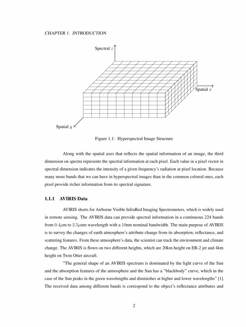
of bands. The hyperspectral data is organized in a three-dimensional structure, and Figure 1.1 showed
the features of this kind of structure.
1
CHAPTER 1. INTRODUCTION
Spatial x
Spectral z
Spatial y
Figure 1.1: Hyperspectral Image Structure
Along with the spatial axes that reflects the spatial information of an image, the third
dimension on spectra represents the spectral information at each pixel. Each value in a pixel vector in
spectral dimension indicates the intensity of a given frequency’s radiation at pixel location. Because
many more bands that we can have in hyperspectral images than in the common colored ones, each
pixel provide richer information from its spectral signature.
1.1.1 AVIRIS Data
AVIRIS shorts for Airborne Visible InfraRed Imaging Spectrometers, which is widely used
in remote sensing. The AVIRIS data can provide spectral information in a continuous 224 bands
from 0.4µm to 2.5µnm wavelength with a 10nm nominal bandwidth. The main purpose of AVIRIS
is to survey the changes of earth atmosphere’s attribute change from its absorption, reflectance, and
scattering features. From these atmosphere’s data, the scientist can track the environment and climate
change. The AVIRIS is flown on two different heights, which are 20km height on ER-2 jet and 4km
height on Twin Otter aircraft.
”The general shape of an AVIRIS spectrum is dominated by the light curve of the Sun
and the absorption features of the atmosphere and the Sun has a ”blackbody” curve, which in the
case of the Sun peaks in the green wavelengths and diminishes at higher and lower wavelengths” [1].
The received data among different bands is correspond to the object’s reflectance attributes and
2
CHAPTER 1. INTRODUCTION
atmosphere absorption. At the bands with low transmittance, the spectra curve will be represented
in deep valleys. For example, the valley of many spectra curves around 1.4µm is mainly caused by
vapor and carbon dioxide. The peaks are often caused by the solar radiation, in many spectral curves,
the highest peak is often around a wavelength of 0.53µm where the strongest radiation of sun light
exists. The data is quantized into 10 or 12bits which depends on the date. AVIRIS data covers a
range of NIR and SWIR bands and the system has a 12Hz ”whisk broom” scanning rate with 76GB
storage.
1.1.2 AIRS Data
AIRS stands for Atmospheric Infrared Sounder and is the standard reference in compression
studies of ultraspectral data. It provides a number of 2378 spectral bands from 3.7 to 15.4 microns
and the data is ranging from 12 bits to 14 bits which depending on the bands. The AIRS data covers
the whole self-emitted IR bands. ”The mission of AIRS is to observe and characterize the entire
atmospheric column from the surface to the top of the atmosphere in terms of surface emissivity
and temperature, atmospheric temperature and humidity profiles, cloud amount and height, and the
spectral outgoing infrared radiation” [2].
1.1.3 Reflection Bands
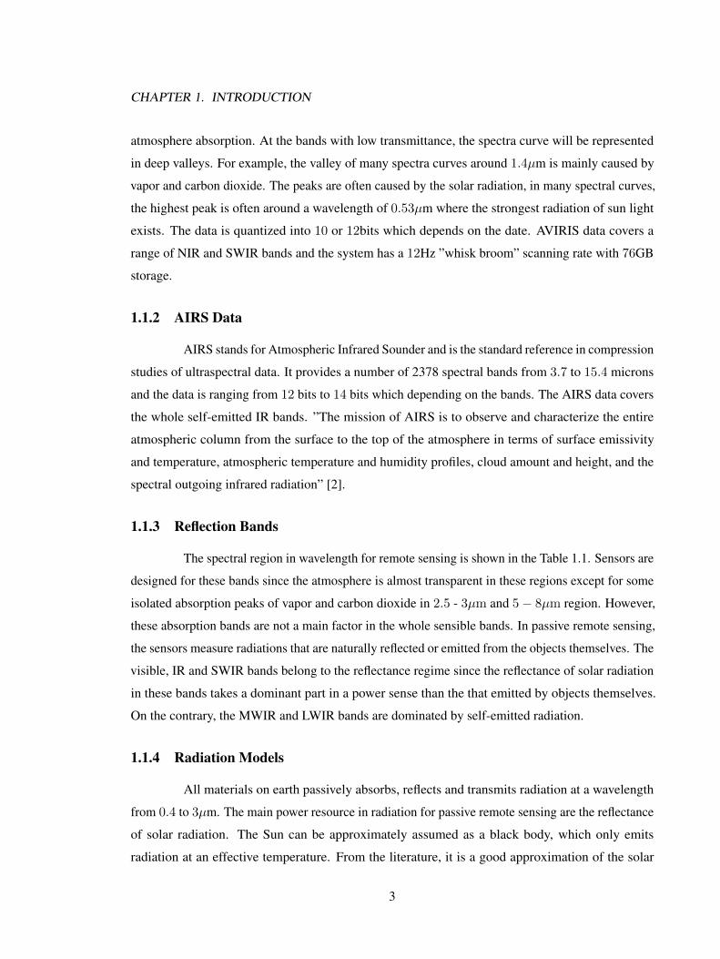
The spectral region in wavelength for remote sensing is shown in the Table 1.1. Sensors are
designed for these bands since the atmosphere is almost transparent in these regions except for some
isolated absorption peaks of vapor and carbon dioxide in 2.5 - 3µm and 5− 8µm region. However,
these absorption bands are not a main factor in the whole sensible bands. In passive remote sensing,
the sensors measure radiations that are naturally reflected or emitted from the objects themselves. The
visible, IR and SWIR bands belong to the reflectance regime since the reflectance of solar radiation
in these bands takes a dominant part in a power sense than the that emitted by objects themselves.
On the contrary, the MWIR and LWIR bands are dominated by self-emitted radiation.
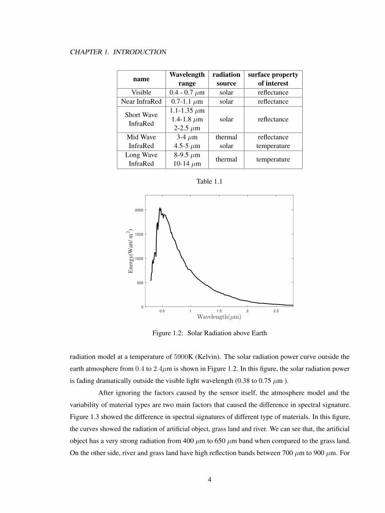
1.1.4 Radiation Models
All materials on earth passively absorbs, reflects and transmits radiation at a wavelength
from 0.4 to 3µm. The main power resource in radiation for passive remote sensing are the reflectance
of solar radiation. The Sun can be approximately assumed as a black body, which only emits
radiation at an effective temperature. From the literature, it is a good approximation of the solar
3
CHAPTER 1. INTRODUCTION
name Wavelengthrange
radiationsource
surface propertyof interest
Visible 0.4 - 0.7 µm solar reflectanceNear InfraRed 0.7-1.1 µm solar reflectance
Short WaveInfraRed
1.1-1.35 µm1.4-1.8 µm2-2.5 µm
solar reflectance
Mid WaveInfraRed
3-4 µm4.5-5 µm
thermalsolar
reflectancetemperature
Long WaveInfraRed
8-9.5 µm10-14 µm
thermal temperature
Table 1.1
0.5 1 1.5 2 2.5
Wavelength(µm)
0
500
1000
1500
2000
En
erg
y(W
att/
m2)
Figure 1.2: Solar Radiation above Earth
radiation model at a temperature of 5900K (Kelvin). The solar radiation power curve outside the
earth atmosphere from 0.4 to 2.4µm is shown in Figure 1.2. In this figure, the solar radiation power
is fading dramatically outside the visible light wavelength (0.38 to 0.75 µm ).
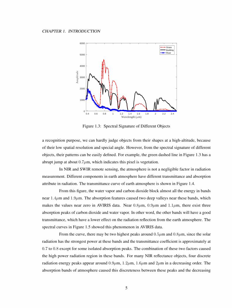
After ignoring the factors caused by the sensor itself, the atmosphere model and the
variability of material types are two main factors that caused the difference in spectral signature.
Figure 1.3 showed the difference in spectral signatures of different type of materials. In this figure,
the curves showed the radiation of artificial object, grass land and river. We can see that, the artificial
object has a very strong radiation from 400 µm to 650 µm band when compared to the grass land.
On the other side, river and grass land have high reflection bands between 700 µm to 900 µm. For
4
CHAPTER 1. INTRODUCTION
0.4 0.6 0.8 1 1.2 1.4 1.6 1.8 2 2.2 2.4Wavelength (µm)
0
1000
2000
3000
4000
5000
6000
Amplitude
GrassBuildingRiver
Figure 1.3: Spectral Signature of Different Objects
a recognition purpose, we can hardly judge objects from their shapes at a high-altitude, because
of their low spatial resolution and special angle. However, from the spectral signature of different
objects, their patterns can be easily defined. For example, the green dashed line in Figure 1.3 has a
abrupt jump at about 0.7µm, which indicates this pixel is vegetation.
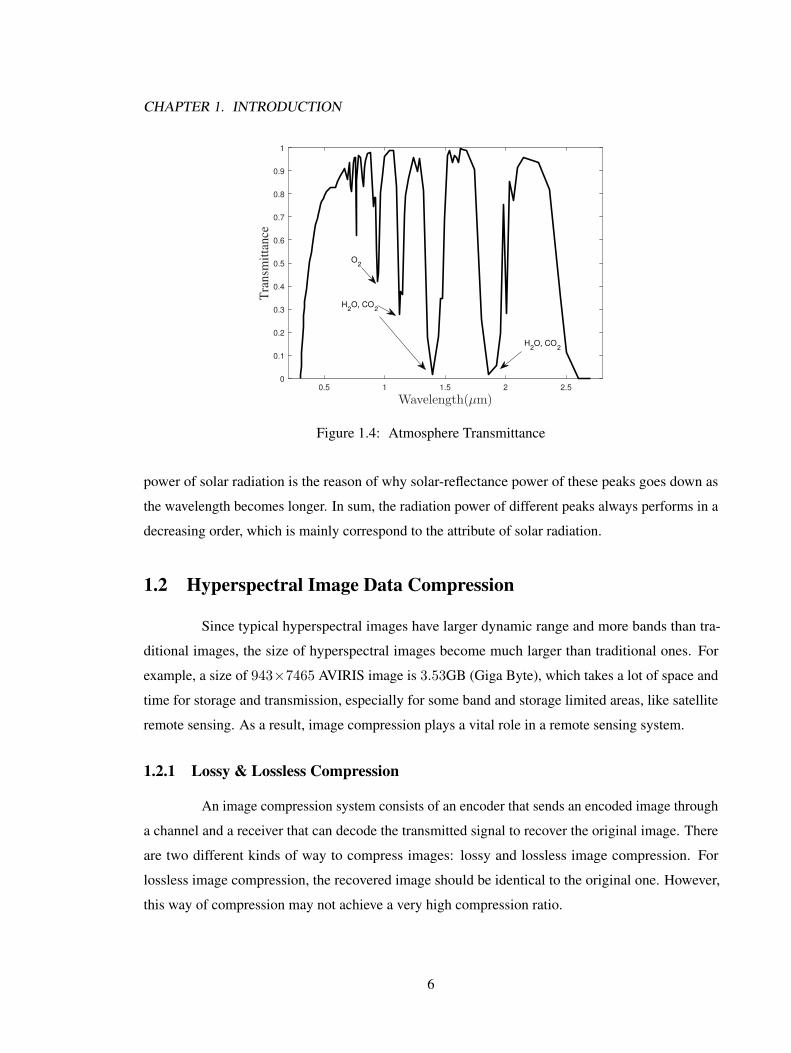
In NIR and SWIR remote sensing, the atmosphere is not a negligible factor in radiation
measurement. Different components in earth atmosphere have different transmittance and absorption
attribute in radiation. The transmittance curve of earth atmosphere is shown in Figure 1.4.
From this figure, the water vapor and carbon dioxide block almost all the energy in bands
near 1.4µm and 1.9µm. The absorption features caused two deep valleys near these bands, which
makes the values near zero in AVIRIS data. Near 0.8µm, 0.9µm and 1.1µm, there exist three
absorption peaks of carbon dioxide and water vapor. In other word, the other bands will have a good
transmittance, which have a lower effect on the radiation reflection from the earth atmosphere. The
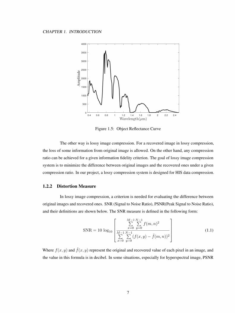
spectral curves in Figure 1.5 showed this phenomenon in AVIRIS data.
From the curve, there may be two highest peaks around 0.5µm and 0.8µm, since the solar
radiation has the strongest power at these bands and the transmittance coefficient is approximately at
0.7 to 0.8 except for some isolated absorption peaks. The combination of these two factors caused
the high power radiation region in these bands. For many NIR reflectance objects, four discrete
radiation energy peaks appear around 0.9µm, 1.2µm, 1.6µm and 2µm in a decreasing order. The
absorption bands of atmosphere caused this discreteness between these peaks and the decreasing
5
CHAPTER 1. INTRODUCTION
0.5 1 1.5 2 2.5
Wavelength(µm)
0
0.1
0.2
0.3
0.4
0.5
0.6
0.7
0.8
0.9
1
Tra
nsm
itta
nce
O2
H2O, CO
2
H2O, CO
2
Figure 1.4: Atmosphere Transmittance
power of solar radiation is the reason of why solar-reflectance power of these peaks goes down as
the wavelength becomes longer. In sum, the radiation power of different peaks always performs in a
decreasing order, which is mainly correspond to the attribute of solar radiation.
1.2 Hyperspectral Image Data Compression
Since typical hyperspectral images have larger dynamic range and more bands than tra-
ditional images, the size of hyperspectral images become much larger than traditional ones. For
example, a size of 943×7465 AVIRIS image is 3.53GB (Giga Byte), which takes a lot of space and
time for storage and transmission, especially for some band and storage limited areas, like satellite
remote sensing. As a result, image compression plays a vital role in a remote sensing system.
1.2.1 Lossy & Lossless Compression
An image compression system consists of an encoder that sends an encoded image through
a channel and a receiver that can decode the transmitted signal to recover the original image. There
are two different kinds of way to compress images: lossy and lossless image compression. For
lossless image compression, the recovered image should be identical to the original one. However,
this way of compression may not achieve a very high compression ratio.
6
CHAPTER 1. INTRODUCTION
0.4 0.6 0.8 1 1.2 1.4 1.6 1.8 2 2.2 2.4
Wavelength(µm)
0
500
1000
1500
2000
2500
3000
3500
4000
Am
pli
tud
e
Figure 1.5: Object Reflectance Curve
The other way is lossy image compression. For a recovered image in lossy compression,
the loss of some information from original image is allowed. On the other hand, any compression
ratio can be achieved for a given information fidelity criterion. The goal of lossy image compression
system is to minimize the difference between original images and the recovered ones under a given
compression ratio. In our project, a lossy compression system is designed for HIS data compression.
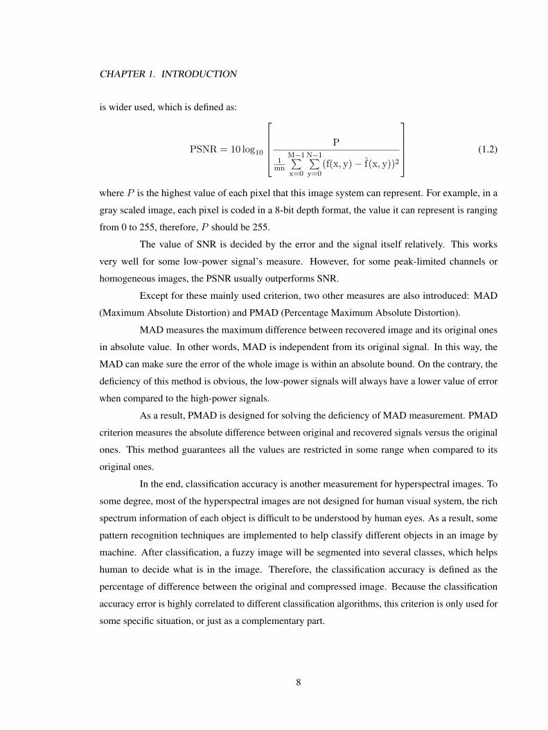
1.2.2 Distortion Measure
In lossy image compression, a criterion is needed for evaluating the difference between
original images and recovered ones. SNR (Signal to Noise Ratio), PSNR(Peak Signal to Noise Ratio),
and their definitions are shown below. The SNR measure is defined in the following form:
SNR = 10 log10
M−1∑x=0
N−1∑y=0
f(m,n)2
M−1∑x=0
N−1∑y=0
(f(x, y)− f(m,n))2
(1.1)
Where f(x, y) and f(x, y) represent the original and recovered value of each pixel in an image, and
the value in this formula is in decibel. In some situations, especially for hyperspectral image, PSNR
7
CHAPTER 1. INTRODUCTION
is wider used, which is defined as:
PSNR = 10 log10
P
1mn
M−1∑x=0
N−1∑y=0
(f(x, y)− f(x, y))2
(1.2)
where P is the highest value of each pixel that this image system can represent. For example, in a
gray scaled image, each pixel is coded in a 8-bit depth format, the value it can represent is ranging
from 0 to 255, therefore, P should be 255.
The value of SNR is decided by the error and the signal itself relatively. This works
very well for some low-power signal’s measure. However, for some peak-limited channels or
homogeneous images, the PSNR usually outperforms SNR.
Except for these mainly used criterion, two other measures are also introduced: MAD
(Maximum Absolute Distortion) and PMAD (Percentage Maximum Absolute Distortion).
MAD measures the maximum difference between recovered image and its original ones
in absolute value. In other words, MAD is independent from its original signal. In this way, the
MAD can make sure the error of the whole image is within an absolute bound. On the contrary, the
deficiency of this method is obvious, the low-power signals will always have a lower value of error
when compared to the high-power signals.
As a result, PMAD is designed for solving the deficiency of MAD measurement. PMAD
criterion measures the absolute difference between original and recovered signals versus the original
ones. This method guarantees all the values are restricted in some range when compared to its
original ones.
In the end, classification accuracy is another measurement for hyperspectral images. To
some degree, most of the hyperspectral images are not designed for human visual system, the rich
spectrum information of each object is difficult to be understood by human eyes. As a result, some
pattern recognition techniques are implemented to help classify different objects in an image by
machine. After classification, a fuzzy image will be segmented into several classes, which helps
human to decide what is in the image. Therefore, the classification accuracy is defined as the
percentage of difference between the original and compressed image. Because the classification
accuracy error is highly correlated to different classification algorithms, this criterion is only used for
some specific situation, or just as a complementary part.
8
CHAPTER 1. INTRODUCTION
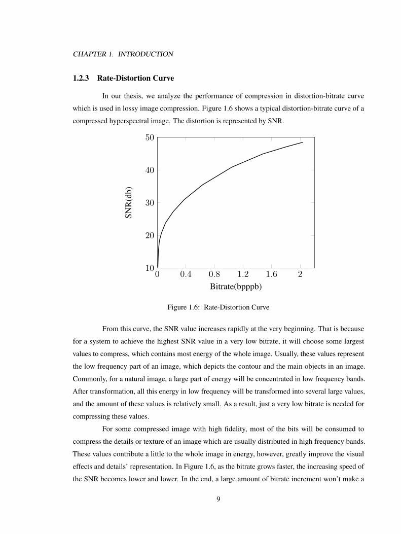
1.2.3 Rate-Distortion Curve
In our thesis, we analyze the performance of compression in distortion-bitrate curve
which is used in lossy image compression. Figure 1.6 shows a typical distortion-bitrate curve of a
compressed hyperspectral image. The distortion is represented by SNR.
0 0.4 0.8 1.2 1.6 210
20
30
40
50
Bitrate(bpppb)
SNR
(db)
Figure 1.6: Rate-Distortion Curve
From this curve, the SNR value increases rapidly at the very beginning. That is because
for a system to achieve the highest SNR value in a very low bitrate, it will choose some largest
values to compress, which contains most energy of the whole image. Usually, these values represent
the low frequency part of an image, which depicts the contour and the main objects in an image.
Commonly, for a natural image, a large part of energy will be concentrated in low frequency bands.
After transformation, all this energy in low frequency will be transformed into several large values,
and the amount of these values is relatively small. As a result, just a very low bitrate is needed for
compressing these values.
For some compressed image with high fidelity, most of the bits will be consumed to
compress the details or texture of an image which are usually distributed in high frequency bands.
These values contribute a little to the whole image in energy, however, greatly improve the visual
effects and details’ representation. In Figure 1.6, as the bitrate grows faster, the increasing speed of
the SNR becomes lower and lower. In the end, a large amount of bitrate increment won’t make a
9
CHAPTER 1. INTRODUCTION
great improvement to the noise reduction. Therefore, for high-fidelity lossy image compression, the
main task is how to compress the scattered high-frequency values in a relatively low bitrate.
1.2.4 Spectral & Spatial Accessibility
Spatial accessibility is an ability that the compression system can access an arbitrary
cropped image without decoding the whole one. In hyperspectral image compression, we generalize
this definition to the spectral dimension, which means the ability to access any cropped image in any
several continuous bands. With this kind of feature, a system can easily access any interested region
in high resolution after getting the low resolution part of the whole image. This ability is very useful
in multi-resolution image processing. For convenience, users can access any part of the image in a
high resolution without decoding the whole image, which is time saving and coding efficiency.
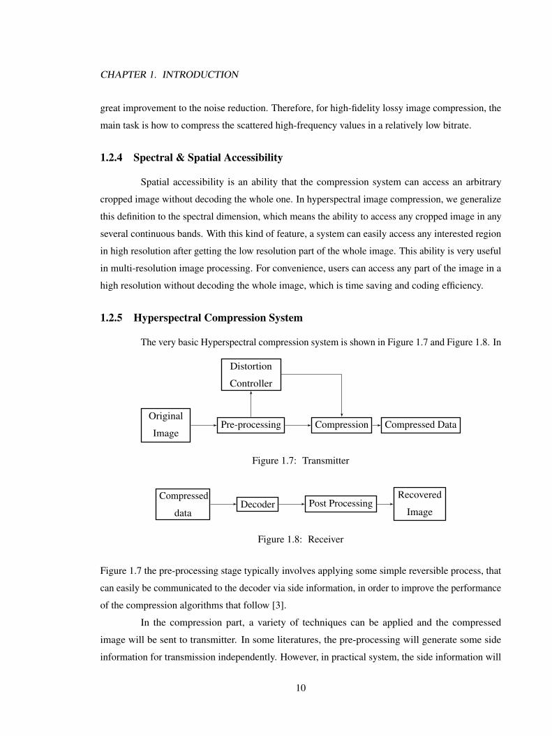
1.2.5 Hyperspectral Compression System
The very basic Hyperspectral compression system is shown in Figure 1.7 and Figure 1.8. In
Original
ImagePre-processing Compression
Distortion
Controller
Compressed Data
Figure 1.7: Transmitter
Compressed
dataDecoder Post Processing
Recovered
Image
Figure 1.8: Receiver
Figure 1.7 the pre-processing stage typically involves applying some simple reversible process, that
can easily be communicated to the decoder via side information, in order to improve the performance
of the compression algorithms that follow [3].
In the compression part, a variety of techniques can be applied and the compressed
image will be sent to transmitter. In some literatures, the pre-processing will generate some side
information for transmission independently. However, in practical system, the side information will
10
CHAPTER 1. INTRODUCTION
be embedded into the compressed image bitstream as control information. Therefore, we organize all
this information together for compression.
At the receiver side, the image content will be decoded firstly and the post processing
part is just the reversed operation of pre-processing part in transmitter side. Based on the quality of
recovered image, it will be used in classification, detection or some other research areas.
1.3 Summary
In this chapter, we introduced the structure of hyperspectral data at the very beginning.
In the following, we discussed spectral signature of hyperspectral images based on the reflectance
attribute of different objects and the transmittance of atmosphere. By taking advantage of the spectral
signature, some process for compression can be applied and this will be specified in the following
chapter. At last, we introduced some criterion to decided the quality for lossy image compression
and a compression system for hyperspectral data is also raised.
11
Chapter 2
Review of Background in Signal Coding
In this chapter we will briefly review coding techniques that are widely used in image or
other media compression. These techniques are used in different application areas based on their
specific features. Some of the wavelet based coding and entropy coding techniques are introduced in
this chapter which are the basis of our proposed compression system.
2.1 Coding Techniques
In this section, spatial transform-domain coding techniques are discussed. Except for
vector quantization, all the other techniques can be applied both for the original data coding and
transformed data coding.
2.1.1 Entropy Coding
The notion of information entropy was firstly introduced by Claude Elwood Shannon,
the founder of information theory. In his work: A Mathematical Theory of Communication [4], he
introduced probability into a communication system. The information that a symbol contains is
correlated to the probability it appears, which is measured by entropy. The formula is:
H[s] =
m∑i=1
pi log2
(1
pi
)(2.1)
where H[s] represents the entropy of signal source, and there are m symbols with a probability of pi
to appear in signal source. As a result, the entropy coding is a approach to maximize the entropy of
each symbol and each symbol in the transmission channel shall be efficiently used. In this section,
12
CHAPTER 2. REVIEW OF BACKGROUND IN SIGNAL CODING
we will briefly review three dominant entropy coding techniques.
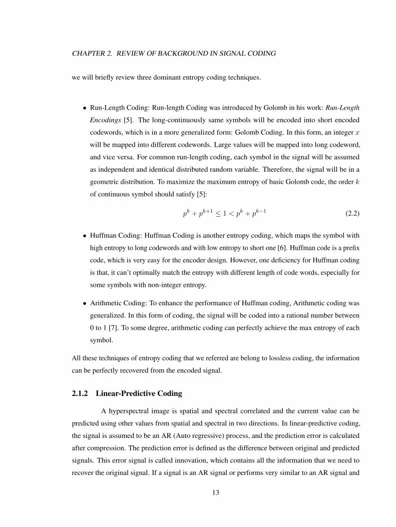
• Run-Length Coding: Run-length Coding was introduced by Golomb in his work: Run-Length
Encodings [5]. The long-continuously same symbols will be encoded into short encoded
codewords, which is in a more generalized form: Golomb Coding. In this form, an integer x
will be mapped into different codewords. Large values will be mapped into long codeword,
and vice versa. For common run-length coding, each symbol in the signal will be assumed
as independent and identical distributed random variable. Therefore, the signal will be in a
geometric distribution. To maximize the maximum entropy of basic Golomb code, the order k
of continuous symbol should satisfy [5]:
pk + pk+1 ≤ 1 < pk + pk−1 (2.2)
• Huffman Coding: Huffman Coding is another entropy coding, which maps the symbol with
high entropy to long codewords and with low entropy to short one [6]. Huffman code is a prefix
code, which is very easy for the encoder design. However, one deficiency for Huffman coding
is that, it can’t optimally match the entropy with different length of code words, especially for
some symbols with non-integer entropy.
• Arithmetic Coding: To enhance the performance of Huffman coding, Arithmetic coding was
generalized. In this form of coding, the signal will be coded into a rational number between
0 to 1 [7]. To some degree, arithmetic coding can perfectly achieve the max entropy of each
symbol.
All these techniques of entropy coding that we referred are belong to lossless coding, the information
can be perfectly recovered from the encoded signal.
2.1.2 Linear-Predictive Coding
A hyperspectral image is spatial and spectral correlated and the current value can be
predicted using other values from spatial and spectral in two directions. In linear-predictive coding,
the signal is assumed to be an AR (Auto regressive) process, and the prediction error is calculated
after compression. The prediction error is defined as the difference between original and predicted
signals. This error signal is called innovation, which contains all the information that we need to
recover the original signal. If a signal is an AR signal or performs very similar to an AR signal and
13
CHAPTER 2. REVIEW OF BACKGROUND IN SIGNAL CODING
wn
1
1+d∑
n=1anzn
+
-d∑
n=0anz
n
Colored Filter
Predictor
enWhite Noise
yn
yn
yn
Innovation
Figure 2.1: Predictive Coding System
the prediction process is well-designed, the original signal can be transformed into innovation with a
low dynamic range, which is very easy to be compressed
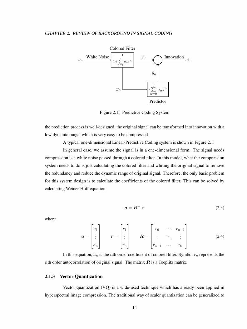
A typical one-dimensional Linear-Predictive Coding system is shown in Figure 2.1:
In general case, we assume the signal is in a one-dimensional form. The signal needs
compression is a white noise passed through a colored filter. In this model, what the compression
system needs to do is just calculating the colored filter and whiting the original signal to remove
the redundancy and reduce the dynamic range of original signal. Therefore, the only basic problem
for this system design is to calculate the coefficients of the colored filter. This can be solved by
calculating Weiner-Hoff equation:
a = R−1r (2.3)
where
a =
a1...
an
r =
r1...
rn
R =
r0 · · · rn−1...
. . ....
rn−1 · · · r0
(2.4)
In this equation, an is the nth order coefficient of colored filter. Symbol rn represents the
nth order autocorrelation of original signal. The matrix R is a Toeplitz matrix.
2.1.3 Vector Quantization
Vector quantization (VQ) is a wide-used technique which has already been applied in
hyperspectral image compression. The traditional way of scaler quantization can be generalized to
14
CHAPTER 2. REVIEW OF BACKGROUND IN SIGNAL CODING
vector quantization. From the work of G.Motton and F.Rizzon [8], we can define the system for
vector quantization:
A kind of transform T is needed for mapping each vector to another one. In a compression
sense, the total number of transformed vector should be far less than the original ones. So that, the
transform T should be a low rank matrix.
From above, VQ belongs to lossy image compression, and after quantization, the original
signal can’t be perfectly recovered. Some information will be lost. Such that, the quantized vectors
should be carefully selected to achieve the least information loss with competitive compression ratio.
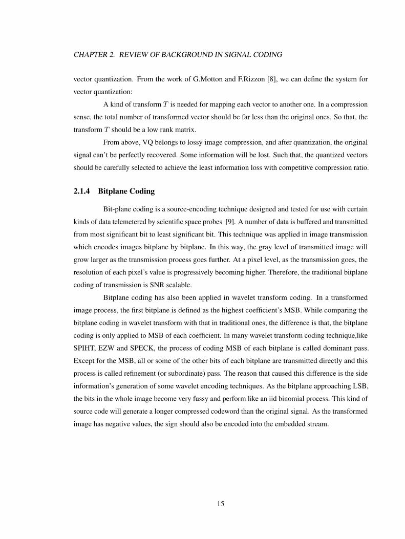
2.1.4 Bitplane Coding
Bit-plane coding is a source-encoding technique designed and tested for use with certain
kinds of data telemetered by scientific space probes [9]. A number of data is buffered and transmitted
from most significant bit to least significant bit. This technique was applied in image transmission
which encodes images bitplane by bitplane. In this way, the gray level of transmitted image will
grow larger as the transmission process goes further. At a pixel level, as the transmission goes, the
resolution of each pixel’s value is progressively becoming higher. Therefore, the traditional bitplane
coding of transmission is SNR scalable.
Bitplane coding has also been applied in wavelet transform coding. In a transformed
image process, the first bitplane is defined as the highest coefficient’s MSB. While comparing the
bitplane coding in wavelet transform with that in traditional ones, the difference is that, the bitplane
coding is only applied to MSB of each coefficient. In many wavelet transform coding technique,like
SPIHT, EZW and SPECK, the process of coding MSB of each bitplane is called dominant pass.
Except for the MSB, all or some of the other bits of each bitplane are transmitted directly and this
process is called refinement (or subordinate) pass. The reason that caused this difference is the side
information’s generation of some wavelet encoding techniques. As the bitplane approaching LSB,
the bits in the whole image become very fussy and perform like an iid binomial process. This kind of
source code will generate a longer compressed codeword than the original signal. As the transformed
image has negative values, the sign should also be encoded into the embedded stream.
15
CHAPTER 2. REVIEW OF BACKGROUND IN SIGNAL CODING
2.2 Transform Coding
To take advantage of the correlation in a picture’s pixels, transform a image to another
basis will be much easier for compression. Transform coding is nowadays the most wide-used way of
compression. In most cases, the transform matrix T is a full-rank matrix. In other word, the transform
is reversible. After transform, we can make the power of an image to be more concentrated in some
basis, which can’t be better for compression. In this section, several common image transform will
be introduced.
2.2.1 Discrete Cosine Transform
In digital image processing, a very common way to view property of an image is using
Discrete Fourier transform. However, two deficiencies this approach will introduce:
• An image is consisted of real values, as a result, the transformed results will contain complex-
values. This will burden compression system for calculating, representing and transmitting
these kind of complex numbers.
• Implicit n-point periodicity of the DFT introduces boundary discontinuities which result in
additional high-frequency components added to the original signal. ”After quantization, the
Gibbs phenomenon will cause obvious block artifact” [10].
Therefore, DCT (Discrete Cosine Transform) was introduced which can overcome the deficiencies of
DFT. The basis of DCT is to given in the following form:
tω = α(ω) cos
[(2x+ 1)ωπ
2N
](2.5)
α =
√
1N ω = 0√2N ω = 1, 2, 3...., N − 1
(2.6)
From the formula above, the transform basis is shifted to the real domain, and the calculation will be
simplified. Another change is that, the 2N-point periodic tapping method will make the boundary of
each block smoother, which will reduce the block artifact. By doing projections, a function f(x) can
be represented as the coefficients of a set of orthogonal discrete cosine functions, which is:
C(ω) =< f(x), t∗w > (2.7)
16
CHAPTER 2. REVIEW OF BACKGROUND IN SIGNAL CODING
and the form of inversed transform is:
f(x) =N−1∑ω=0
C(ω)tω (2.8)
The basis of DCT has a very strong correlation to the KL decomposition in the first-order Markov
chain. The covariance matrix of the first-order Markov process is given by [11]:
C =
1 ρ ρ2 . . . ρn−1
ρ 1 ρ . . . ρn−2
ρ2 ρ 1 . . . ρn−3
......
.... . .
...
ρn−1 ρn−2 ρn−3 . . . . . .
(2.9)
where ρ is the correlation coefficient. For this matrix, when ρ is approximately 1, the eigenvectors of
this matrix will be very closed to the discrete cosine functions. Besides, most natural images perform
like a first-order Markov process and their correlation is near linear. As a result, the DCT will be a
suboptimal transform in de-correlation and compression.
In sum, DCT is still widely used in our common lives, the daily used standard JPEG is
mainly based this technique. Though some flaws of this technique exist, like block effect in low SNR,
it still performs well in many scenarios.
2.2.2 Discrete Wavelet Transform
Wavelet transform and its theory matured in recent twenty years. Unlike the Fourier
transform only having frequency localization, the wavelet transform has both time and frequency
localization property. A wavelet function should be zero-mean valued and supported in a limited
range. Mathematically speaking, wavelet transform is a process to approximating a function by
double-indexed wavelet functions ψa,b(t) in L2 space:
Ca,b = < ψa,b(t), f∗(t) > =
∫ψa,b(t) f
∗(t) dt (2.10)
where the mother wavelet function is:
ψa,b(t) = |a|−12 ψ
(t− ba
)(2.11)
In this way, the original signal f(t) can be represented as a liner combination of dilated and shifted
mother wavelet function ψa,b(t) and both time and frequency localization are achieve.
17
CHAPTER 2. REVIEW OF BACKGROUND IN SIGNAL CODING
In Mallat’s multi-resolution theory for discrete wavelet transform, the original function
can be decomposed by doing projections on the scaling function φa,b(t) and the mother wavelet
ψa,b(t). Once the scaling function φa.b(t) is decided, its counterpart, ψa,b(t) can be calculated by
doing projections on the scaling function family. In multi-resolution analysis, a functional space
is divided into several laddered part, the function φa,b(t) represents the low-resolution part of the
original signal in this functional space. On the contrary, function ψa,b(t) is the high-resolution part.
The whole discrete wavelet transform can be represented as a process that keep splitting the finer
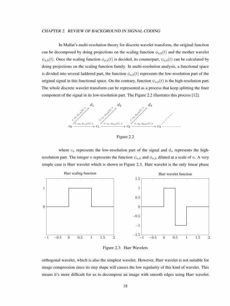
component of the signal in its low-resolution part. The Figure 2.2 illustrates this process [12].
c0
d1
c1
d2
c2
d3
c3< c0, φ1,k(t) >
<c 0, ψ
1,k(t)>
< c1, φ2,k(t) >
<c 1, ψ
2,k(t)>
< c2, φ3,k(t) >
<c 2, φ
3,k(t)>
Figure 2.2
where cn represents the low-resolution part of the signal and dn represents the high-
resolution part. The integer n represents the function ψn,k and φn,k dilated at a scale of n. A very
simple case is Harr wavelet which is shown in Figure 2.3. Harr wavelet is the only linear phase
−1 −0.5 0 0.5 1 1.5 2
0
1
Harr scaling function
−1 −0.5 0 0.5 1 1.5 2−1.5
−1
−0.5
0
0.5
1
1.5Harr wavelet function
Figure 2.3: Harr Wavelets
orthogonal wavelet, which is also the simplest wavelet. However, Harr wavelet is not suitable for
image compression since its step shape will causes the low regularity of this kind of wavelet. This
means it’s more difficult for us to decompose an image with smooth edges using Harr wavelet.
18
CHAPTER 2. REVIEW OF BACKGROUND IN SIGNAL CODING
To achieve both linear phase and regularity, the bi-orthogonal wavelets were invented for image
compression and the wide-known bi-orthogonal wavelets are CDF 9/7 and CDF 5/3 wavelets, which
have already been applied in lossy and lossless image compression in JPEG2000 standard. In the
later chapter, we will clarify how DWT can be implemented using filter banks for hyperspectral
image compression.
2.2.3 KL Transform
In signal processing, ”A signal can be represented in a set of statistically uncorrelated
basis functions on its property of second order random signal” [13]. In this way, the signals can be
transformed into a diagonal matrix which represents each uncorrelated basis in a power sense. This
transform was firstly introduced by Karhunen and Loeve as the Hotelling transform. Assume that, a
zero-mean vector x is a sampled signal needs to be transform. This transform can be represented in
this way:
Rx = KDKT (2.12)
w = KTx (2.13)
where Rx is the autocorrelation matrix of vector x and the matrix K stands for its eigenmatrix which
is unitary. The orthogonal transform in 2.13 generates an uncorrelated vector w who has a zero mean
with autocorrelation D. In practical, x is assumed to be the original signal and the compression can
be achieved by encoding w to w. At the receiver side, the recovered signal x can be recovered by:
x = Kw (2.14)
KL transform is the optimal transform in signal compression, however, its deficiency is also obvious.
Because the KL transform is a data-based transform and the basis should be transmitted for every
image. Another problem is the high computational complexity caused by its basis computation
every time. In sum, KL transform is the best transform theoretically, however, hard to be applied in
practical use.
2.3 Wavelet-based Coding techniques
After performing isotropic DWT to an image, the transformed data will have a pyramidal
structure. For natural images, the coefficients have correlation between each subbands, and this can
19
CHAPTER 2. REVIEW OF BACKGROUND IN SIGNAL CODING
be used to compress these coefficients. The following techniques based on DWT exploited this kind
of correlation, which showed how powerful the DWT is in image compression.
Two main techniques are introduced here, which are EZW and SPIHT. In EZW, the tree
structure for compression was first raised. Later, SPIHT was invented to improve the compression
ration of EZW which gives a more refined way to output compressed symbols.
2.3.1 Embedded Zerotree Wavelet (EZW)
EZW algorithm is firstly introduced by Shapiro in his epoch-marking paper [14]. This
paper showed how powerful the DWT is in image compression. EZW stands for Embedded Zero
Tree coding. By taking advantage of the multi-resolution structure in different level of wavelet
transform, through bitplane coding, the transformed coefficients can be highly compressed.
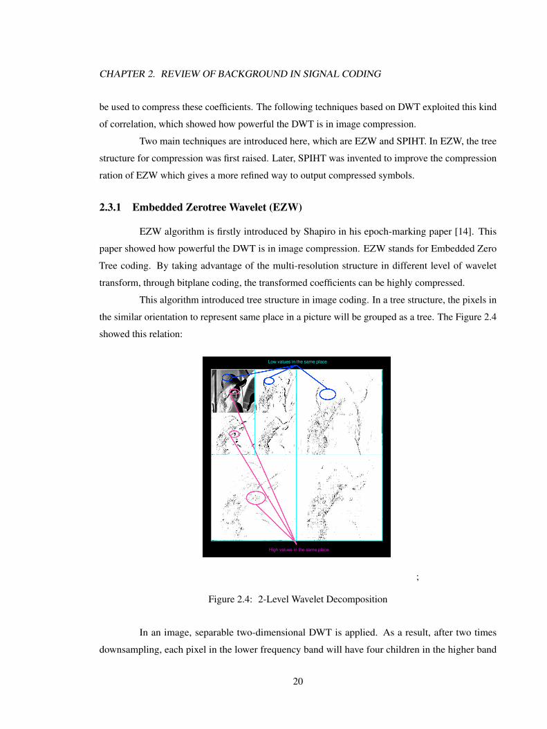
This algorithm introduced tree structure in image coding. In a tree structure, the pixels in
the similar orientation to represent same place in a picture will be grouped as a tree. The Figure 2.4
showed this relation:
Low values in the same place
High values in the same place
;
Figure 2.4: 2-Level Wavelet Decomposition
In an image, separable two-dimensional DWT is applied. As a result, after two times
downsampling, each pixel in the lower frequency band will have four children in the higher band
20
CHAPTER 2. REVIEW OF BACKGROUND IN SIGNAL CODING
in the same frequency direction (except for the highest frequency subbands). In EZW algorithm,
bitplane coding technique is applied. The coding order is from MSB(Most Significan Bit) to
LSB(Least Significant Bit). For each bitplane, all the zeros are coded in a tree structure. The EZW
algorithm takes advantage of the correlation between wavelet coefficients from different subbands
who represent the same place in the original picture. It used the value of a tree root to predict its
leaves. If in one typical bitplane, the root and its leaves are all 0, then, a bunch of all these coefficients
in this tree will be coded into only one symbol. There are four symbols in EZW algorithm to represent
the pixels in each bitplane. They are: P (Positive Significant), N (Negative Significant), I (Isolated
Zero) and R (Zero Tree Root). After zero tree coding, all these symbols are compressed again in
entropy coding for further transmission.
2.3.2 Wavelet Difference Reduction (WDR)
In this algorithm, each pixel are assigned a position number in a baseline scan order.
In such way, the significant bits of each bitplane can be represented in position numbers and the
compression process is performed on these numbers. For natural images, the large coefficients always
concentrate in low frequency bands and are close to each other. Such that, to reduce the dynamic
range of position number for a better compression result, only the difference of position numbers are
encoded. WDR algorithm has a much lower computational complexity than EZW and achieves a
better visual effect under the same compression ratio. This method is more commonly used in the
areas like underwater communication where the transmission speed is limited.
2.3.3 Set Partitioning In Hierarchical Trees (SPIHT)
The SPIHT algorithm was introduced by Said and Pearlman [15]. It is very similar to the
EZW algorithm, however, this algorithm discards the notion of Zero Tree, It uses a hierarchical tree
structure. Because SPIHT is the algorithm that we used in our compression system, some more
details of this algorithm are introduced here.
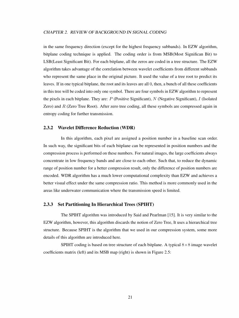
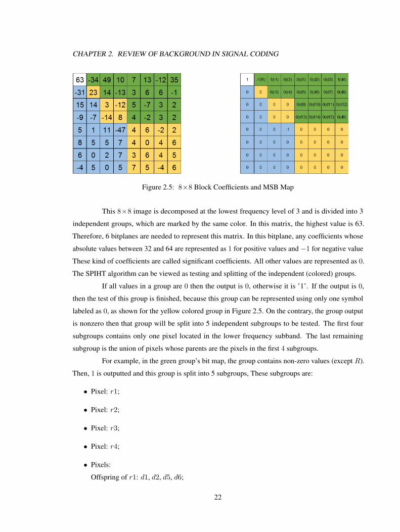
SPIHT coding is based on tree structure of each bitplane. A typical 8×8 image wavelet
coefficients matrix (left) and its MSB map (right) is shown in Figure 2.5:
21
CHAPTER 2. REVIEW OF BACKGROUND IN SIGNAL CODING
Figure 2.5: 8×8 Block Coefficients and MSB Map
This 8×8 image is decomposed at the lowest frequency level of 3 and is divided into 3
independent groups, which are marked by the same color. In this matrix, the highest value is 63.
Therefore, 6 bitplanes are needed to represent this matrix. In this bitplane, any coefficients whose
absolute values between 32 and 64 are represented as 1 for positive values and −1 for negative value
These kind of coefficients are called significant coefficients. All other values are represented as 0.
The SPIHT algorithm can be viewed as testing and splitting of the independent (colored) groups.
If all values in a group are 0 then the output is 0, otherwise it is ’1’. If the output is 0,
then the test of this group is finished, because this group can be represented using only one symbol
labeled as 0, as shown for the yellow colored group in Figure 2.5. On the contrary, the group output
is nonzero then that group will be split into 5 independent subgroups to be tested. The first four
subgroups contains only one pixel located in the lower frequency subband. The last remaining
subgroup is the union of pixels whose parents are the pixels in the first 4 subgroups.
For example, in the green group’s bit map, the group contains non-zero values (except R).
Then, 1 is outputted and this group is split into 5 subgroups, These subgroups are:
• Pixel: r1;
• Pixel: r2;
• Pixel: r3;
• Pixel: r4;
• Pixels:
Offspring of r1: d1, d2, d5, d6;
22
CHAPTER 2. REVIEW OF BACKGROUND IN SIGNAL CODING
Offspring of r2: d3, d4, d7, d8;
Offspring of r3: d9, d10, d13, d14;
Offspring of r4: d11, d12, d15, d16;
Then a set of new tests will be applied to these subgroups. Here we found that, d4 is 1. Hence,
symbol 1 is the output of the last subgroup. Because the last subgroup is in the highest frequency
level, this subgroup will only be divided into four subsubgroups based on the pixels in this subgroup
of their parents and another test will be applied. These four divided subsubgroups are:
• Pixel: d1, d2, d5, d6 (Offspring of r1);
• Pixel: d3, d4, d7, d8 (Offspring of r2);
• Pixel: d9, d10, d13, d14 (Offspring of r3);
• Pixel: d11, d12, d15, d16 (Offspring of r4);
This procedure will repeat until the output is 0 or the groups can’t be divided anymore.
The procedure that we referred above is called dominant pass in SPIHT coding. Next, the
significant coefficients will be sent to the refinement pass for a finer quantization in order to achieve
a better recovery in which the quantization bits are adaptive.
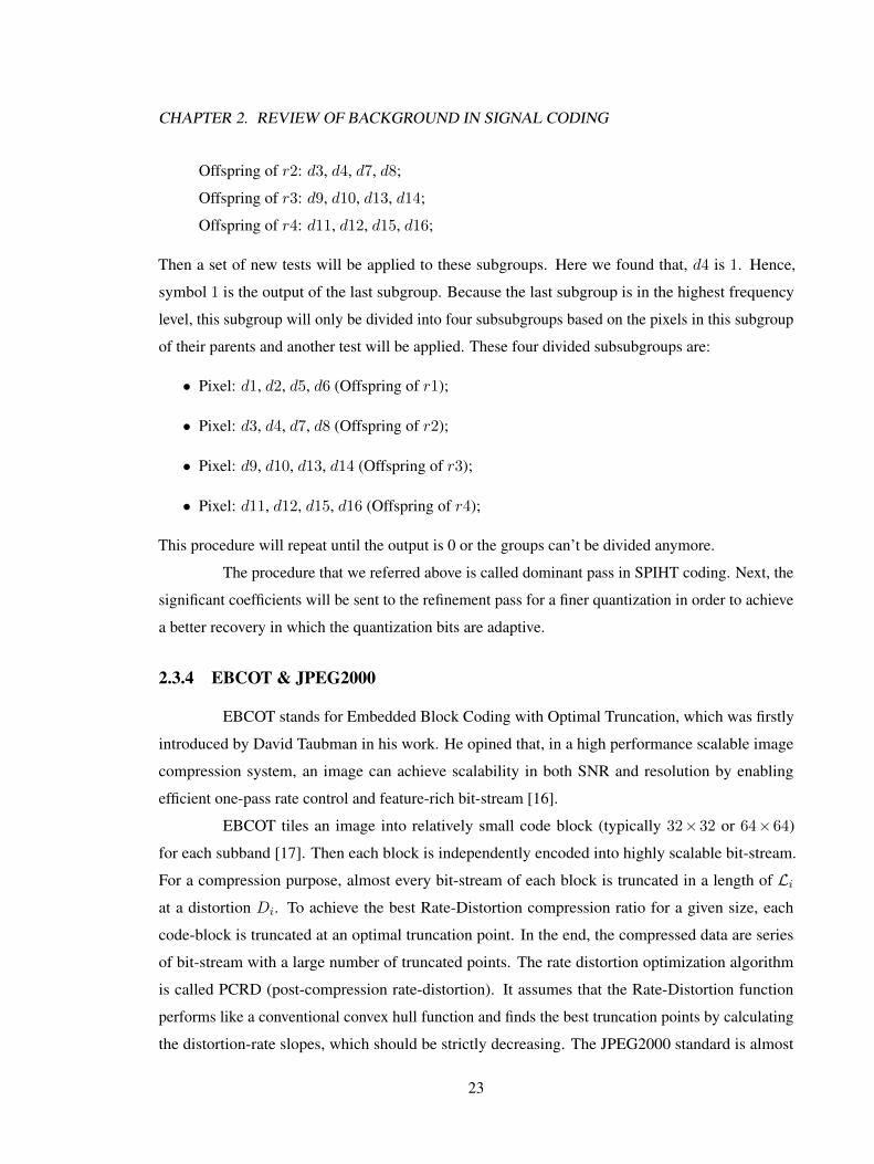
2.3.4 EBCOT & JPEG2000
EBCOT stands for Embedded Block Coding with Optimal Truncation, which was firstly
introduced by David Taubman in his work. He opined that, in a high performance scalable image
compression system, an image can achieve scalability in both SNR and resolution by enabling
efficient one-pass rate control and feature-rich bit-stream [16].
EBCOT tiles an image into relatively small code block (typically 32×32 or 64×64)
for each subband [17]. Then each block is independently encoded into highly scalable bit-stream.
For a compression purpose, almost every bit-stream of each block is truncated in a length of Liat a distortion Di. To achieve the best Rate-Distortion compression ratio for a given size, each
code-block is truncated at an optimal truncation point. In the end, the compressed data are series
of bit-stream with a large number of truncated points. The rate distortion optimization algorithm
is called PCRD (post-compression rate-distortion). It assumes that the Rate-Distortion function
performs like a conventional convex hull function and finds the best truncation points by calculating
the distortion-rate slopes, which should be strictly decreasing. The JPEG2000 standard is almost
23
CHAPTER 2. REVIEW OF BACKGROUND IN SIGNAL CODING
based on EBCOT. The difference is that, the JPEG2000 standard enhances the compression speed at
a cost of relatively low SNR performance by using a fast but less optimal arithmetic encoder, which
reduces the code block size by reducing the fractional bitplane path [17].
2.4 Proposed Algorithm
Recent works in hyperspectral image compression paid much attention to the modification
of decomposition levels for each dimension and the patronized tree design. However, in our algorithm,
we refocused on the classic DCT, which we claim is better for hyperspectral image compression. In
the compression stage, combination of traditional DCT with 3D-SPIHT coding outperforms the DWT
with 3D-SPIHT coding in most situations. This superior performance over traditional DCT-based
JPEG algorithm is obtained carefully choosing block-size and level-shifting
In this thesis, we propose a novel architecture for solving the AVIRIS hyperspectral image
compression problem. In our approach, a hyperspectral image cube is first tiled into many small
cubes on which the subsequent encoding and decoding techniques are applied. Then, These include
3D-DCT transformation, EBCOT-based quantization and 3D-SPIHT algorithm to fulfill our goal.
Because all the operations are based on independent cubes, parallel computing can be
applied in this system. The details of this system architecture are described in the next chapter.
To achieve these goals, we have specified and solved the problems of 3D-SPIHT generalization
including the choice of code cube size.
2.5 Summary
In this chapter, we briefly reviewed some techniques that have already been applied in
media compression. Some of the wavelet based compression algorithms are specified here which
are the basis of this thesis. In practical implementations, a typical encoder/decoder implements not
just one algorithm but a combination of several of them. Usually, the entropy coding and transform
coding always work together to form the main part of the encoder and this structure is also applied in
our proposed system.
24
Chapter 3
Architecture Details
In Chapter 2, the 2D-SPIHT algorithm is introduced. For multi-dimensional images in HSI
data cube, a three-dimensional form of SPIHT (3D-SPIHT) algorithm is described in this chapter.
Here, we specified the details of the 3D-SPIHT algorithm and the tiling strategy for DWT and DCT
cube transform in AVIRIS data. Some basic performance evaluations of the SPIHT algorithm are
also introduced in this chapter, which will help us analyze the compression results in Chapter 5.
3.1 3D-SPIHT
Xiaoli and William in their work [18] firstly presented a new 3D-SPIHT and 3D-SPECK
algorithm for hyperspectral images and showed good results using wavelet transform.
In this section, we introduce this 3D-SPIHT algorithm, which is generalized from tradi-
tional 2D-SPIHT algorithm. We first discuss how a code cubes is set up along with parent-children
relationship between different subbands. We then present the main body of this algorithm.
3.1.1 Code-Block Introduction
From what we introduced in Chapter 2, the hyperspectral data is organized in a three
dimensional cube structure. Therefore, the coding unit is based on a three dimensional cube. Here,
we call the smallest coding as unit code cube. An entire hyperspectral image is tiled into many
cubes and all these cubes can be encoded independently. After three-dimensional dyadic DWT, the
code-cube will be divided into a 3D-pyramidal structure, which is in a frequency domain from lowest
subband to highest subband. The level of the pyramid is decided by DWT decomposition level. The
25
CHAPTER 3. ARCHITECTURE DETAILS
Horizontal
Vertical
Spectr
um
high frequencylow frequency
high fre
quen
cy
lowfre
quen
cy
low
frequency
high
frequency
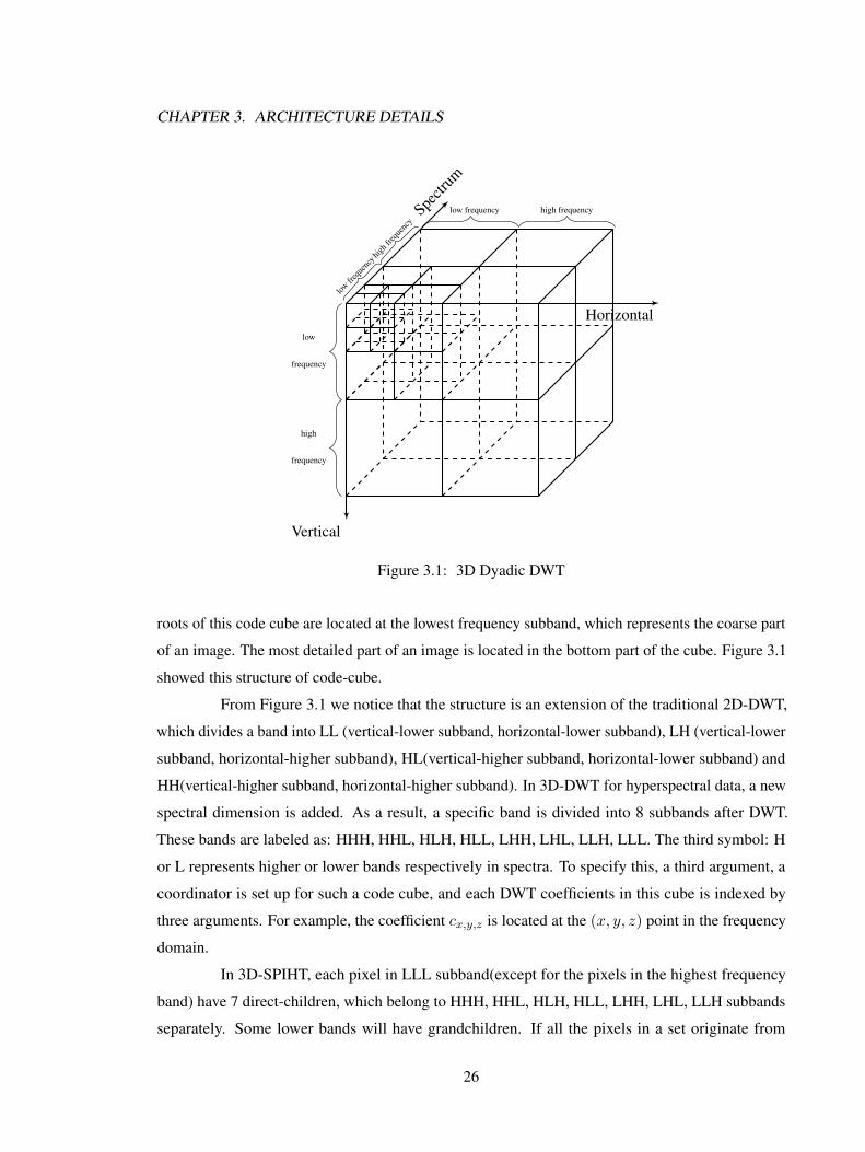
Figure 3.1: 3D Dyadic DWT
roots of this code cube are located at the lowest frequency subband, which represents the coarse part
of an image. The most detailed part of an image is located in the bottom part of the cube. Figure 3.1
showed this structure of code-cube.
From Figure 3.1 we notice that the structure is an extension of the traditional 2D-DWT,
which divides a band into LL (vertical-lower subband, horizontal-lower subband), LH (vertical-lower
subband, horizontal-higher subband), HL(vertical-higher subband, horizontal-lower subband) and
HH(vertical-higher subband, horizontal-higher subband). In 3D-DWT for hyperspectral data, a new
spectral dimension is added. As a result, a specific band is divided into 8 subbands after DWT.
These bands are labeled as: HHH, HHL, HLH, HLL, LHH, LHL, LLH, LLL. The third symbol: H
or L represents higher or lower bands respectively in spectra. To specify this, a third argument, a
coordinator is set up for such a code cube, and each DWT coefficients in this cube is indexed by
three arguments. For example, the coefficient cx,y,z is located at the (x, y, z) point in the frequency
domain.
In 3D-SPIHT, each pixel in LLL subband(except for the pixels in the highest frequency
band) have 7 direct-children, which belong to HHH, HHL, HLH, HLL, LHH, LHL, LLH subbands
separately. Some lower bands will have grandchildren. If all the pixels in a set originate from
26
CHAPTER 3. ARCHITECTURE DETAILS
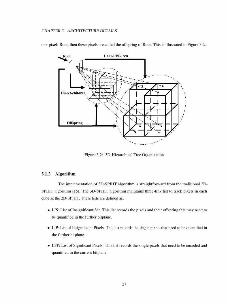
one-pixel: Root, then these pixels are called the offspring of Root. This is illustrated in Figure 3.2.
Root Grandchildren
Direct-c
Offspring
Figure 3.2: 3D-Hierarchical Tree Organization
3.1.2 Algorithm
The implementation of 3D-SPIHT algorithm is straightforward from the traditional 2D-
SPIHT algorithm [15]. The 3D-SPIHT algorithm maintains three-link list to track pixels in each
cube as the 2D-SPIHT. These lists are defined as:
• LIS: List of Insignificant Set. This list records the pixels and their offspring that may need to
be quantified in the further bitplane.
• LIP: List of Insignificant Pixels. This list records the single pixels that need to be quantified in
the further bitplane.
• LSP: List of Significant Pixels. This list records the single pixels that need to be encoded and
quantified in the current bitplane.
27
CHAPTER 3. ARCHITECTURE DETAILS
To develop these list a judgment function is defined below:
J(I) =
1 if max
cx,y,z∈I(|cx,y,z| ≥ T )
0 if maxcx,y,z∈I
(|cx,y,z| < T )(3.1)
where T represents some predefined threshold. Also a new sign function is defined, which maps
values to two symbols:
sgn(cx,y,z) =
+ if cx,y,z ≥ T
− if cx,y,z < −T(3.2)
In bitplane coding, T is commonly chosen as 2n (where n is a positive integer). The set I consists of
values cx,y,z from different locations in a cube.
For representing the hierarchical trees by tracking their root pixels, we define the following
sets:
• O(cx,y,z): Set contains all the offspring of cx,y,z .
• C(cx,y,z): Set contains all the direct-children of cx,y,z . For convenience, we refer to this set as
type B set.
• G(cx,y,z): Set contains and all the grandchildren of cx,y,z which is O(cx,y,z)− C(xx,y,z). we
refer to this set as type A set
A pixel is called significant if its transformed value is larger than the threshold T , otherwise, it is
called insignificant. If the MSB of this transformed value is 1 in its bitplane, the pixel should belong
to significant value set and vice versa. Before the algorithm begins, the link-list and the threshold
values are initialized as:
T ⇐ 2dlog2(max(O(c0,0,0)))e (3.3)
LIP⇐ H (3.4)
LIS⇐ H(type A). (3.5)
The algorithm in Dominant Pass is given in Algorithm 1.
28
CHAPTER 3. ARCHITECTURE DETAILS
After dominant pass, all the values in the LSP are quantified in some bit-depth on the
required reconstruction quality. This procedure is termed as the subordinate path which is given in
Algorithm 2.
From Algorithm 1, every time the threshold T refreshes, a new coding path is created on
LIS. The procedure that completes encoding one bitplane is called a stage of the SPIHT algorithm,
which finishes line 3 to line 34 in Algorithm 1. In each stage, the coefficients whose value are larger
than the threshold are coded and quantized. If the transform is an orthogonal transform, then at the
decoder side, the error between original image and recovered image will become smaller and smaller.
resulting in larger SNR values. Therefore, the SPIHT algorithm is a SNR scalable algorithm which
progressively enhances the SNR of a recovered image through the transmitted bitstream. From the
feature of Rate-Distortion curve in Section 1.2.3, we can infer that, the Rate-Distortion curve of
SPIHT algorithm will increase dramatically during the very first stages. However, as the threshold
becomes smaller, enhancing the compression ratio will be much harder than to achieve than during
the first several stages
3.2 SPIHT Performance Evaluation
In this section, we simplify some coding cases and analyze the performance of 2D-SPIHT
coding algorithm mathematically. The only difference between the 2D and the 3D SPIHT algorithm
is just the number of children of each root. Therefore, the conclusions we derived in this section are
also applicable in the 3D-SPIHT which will help us better analyze the results on the SPIHT coding
performance in different scenarios.
As the coding cost in dominant pass contributes greater than the subordinate pass, the
codeword we discussed here indicates that in the dominant pass only. The performance of the SPIHT
coding wholly depends on the arrangement of different bitplanes. We give the following definition to
form a general case:
Definition 3.1. A finite-ordered sequence of sets on one dimensional space is labeled as:
S1,S2,S3, ....Sk
and all these sets should satisfy: There always exists an onto function fj , such that,
fj : Sj → Sj+1 ⊕ Sj+2 ⊕ Sj+3...⊕ Sk (3.6)
where ⊕ is the symbol of direct sum.
29
CHAPTER 3. ARCHITECTURE DETAILS
The hierarchical trees in wavelet coding can be generated from these sets and the mapping
rule. In hierarchical trees, all the transformed coefficients in a specific level of subband can be
grouped in a set labeled as Si. The index i indicates which level of subband these transformed
coefficients belongs to. The mapping rule illustrates the relationship between different roots and
descendants. With these sets and mapping rules, the tree structure can be transformed into onto
functions between several ordered sets. For instance, in a 2D-DWT image (all the word: image in this
section is defined as transformed image), the coefficients in the lowest frequency level are marked as
the elements in S1, and the coefficients in the higher frequency level belong to S2 and so on.
Here we define that, Si only contains all the coefficients’ absolute value in ith level of
DWT. The integer ni indicates the number of elements in set Si and k is the maximum level of DWT
that is used. All the elements in the lower level are mapped to the elements in higher level which are
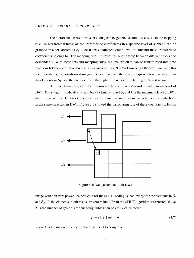
in the same direction in DWT. Figure 3.3 showed the patronizing rule of these coefficients. For an
S1
S2
S3
Figure 3.3: Set patronization in DWT
image with non-zero power, the best case for the SPIHT coding is that, except for the elements in S1and S2, all the elements in other sets are zero-valued. From the SPIHT algorithm we referred above,
T is the number of symbols for encoding, which can be easily calculated as:
T = (k + 1)n2 + n1 (3.7)
where k is the max number of bitplanes we need to compress.
30
CHAPTER 3. ARCHITECTURE DETAILS
Now, let’s consider a worse case: All the sets have a random value for each element,
however, they also satisfied the following rule:
For any elements ei in ith set Si (except for elements in S1),
2blogmin(Si−1)
2 c−1 < ei ≤ 2blogmin(Si−1)
2 c (3.8)
For encoding all the coefficients in SPIHT algorithm, a number of:
Tk = 5n2 +
k−2∑i=3
5ni + 2nk−1 + nk + n1 (3.9)
symbols are needed at most. For convenience, this situation is termed as: Case A. We can prove that
the coding length for a single element in LIS from Sn can be represented in a recursive function:
Y [i] = 4Y [i+ 1] + 5 (3.10)
where 2 ≤ i < k − 1 and Y [k − 1] = 6.
For most natural images, the coefficients’ value decreases very fast in the first several levels
of subbands. In these subbands, most of the coefficients obey the formula in 3.8 and the length of
codeword in these subbands is very short which is still acceptable when compared to the best case.
Now, the situation in the last several subbands becomes worse. The coefficients in the
higher frequency bands have higher values than the lower frequency bands in some cases. Consider
this kind of situation: In an SPIHT coding process, all the elements’ values are the same as that in
Case A, except for one element eck in Sk (the highest frequency subbands), whose value is the same
as someone in S1 (the lowest frequency subbands). For convenience, we termed this situation as:
Case B. To better represent the encoding cost, we introduce the following recursive function:
X[i] = 3Y [i+ 1] +X[i+ 1] + 4(i+ 1) + 2 (3.11)
where 2 ≤ i < k − 1 and X[k − 1] = 3k + 2.
In formula 3.11, X[n] stands for the coding length for encoding a single element ei in LIS
from Si, and eck ∈ fik(ei) (where k is the maximum level of DWT that is used).
Now, let’s consider the difference on coding length for these two different cases:
X[i]− Y [i] = X[i+ 1]Y [i+ 1] + 4(i+ 1)− 3 (3.12)
If we define: C[i] = X[i]− Y [i], formula 3.12 can be written in the following form:
C[i] = C[i+ 1] + 4(i+ 1)− 3 (3.13)
31
CHAPTER 3. ARCHITECTURE DETAILS
where 1 ≤ i < k, therefore C[1] > 0 and sequence C[i] shall be a positive-increasing sequence.
From the result above, the encoding cost in Case B is higher than that in Case A.
Now, let’s take Case C into consideration. In Case C, the situation becomes worse. We
assume that, there is another element c′ck in Sk which shares the same value as cck. For some positive
integer m, there exist two different elements cm, c′m in Sm and an element cm−1 in Sm−1, such
that cck ∈ fmk(cm), c′ck ∈ fmk(c′m), c′ck ∈ fm−1k(cm−1) and cck ∈ fm−1k(cm−1). In traditional
SPIHT image coding, the integer m is a measurement of distance in space between cck and c′ck,
which indicates the level where the two coefficients were separated into two trees.
In Case C, the coding length Z[i] can be represented in the following recursive function
set: Z[i] = 3Y [i+ 1] + Z[i+ 1] + 4(i+ 1) + 2 i < m
Z[i] = 2Y [i+ 1] + 2X[i+ 1] + 8(i+ 1) + 4 i ≥ m(3.14)
The difference on coding length between Case B and Case C shall be:Z[i]−X[i] = Z[i+ 1]−X[i+ 1] i < m
Z[i]−X[i] = C[i+ 1] + 4(i+ 1) + 2 i ≥ m(3.15)
where C[i + 1] > 0, i > 1. The function is a positive-increasing function. Therefore, the coding
cost in Case C is higher than that in case B, and smaller the m higher the coding cost we have. In an
image compression, it will be better for the SPIHT coding if the large valued coefficients in same
frequency bands are concentrated in space. For a more general case, if there are more elements like
ck that exist in the highest frequency level, the recursive function set can be written in:
Z[i] = (4− r)Y [i+ 1] + rX[i+ 1] + r(i+ 1) + 2r mr+1 > i ≥ mr (3.16)
where r is an integer ranging from 1 to 4, which indicates the number of significant values of an
element’s children.
For some more general cases, these recursive functions can be applied to the roots in
LIS respectively and calculation of the codeword length will become more complex. However, the
following conclusions are obvious:
1. Lower values in high-frequency bands results in better compression performance.
2. Many large-valued coefficients group as clusters in the same subbands results in better com-
pression performance than which scatter in the same sabbands.
These conclusions will be used in the following analysis in Chapter 5.
32
CHAPTER 3. ARCHITECTURE DETAILS
3.3 Cube Transformation & Organization
For the purpose of compression, two different kinds of transforms are selected. In this
section, we firstly introduced how the tiled blocks are transformed. Then, we talked about how to tile
the blocks in a spectral sense.
3.3.1 3D-DCT
The transformation of a single block in DCT is very simple, which can be derived from the
one dimensional form. The transformed coefficient I(ω, µ, γ) in 3D-DCT formula is shown below:
I(ω, µ, γ) =M−1∑x=0
N−1∑y=0
S−1∑z=0
I(x, y, z)α(ω)α(µ)α(γ) cos(2x+ 1)ωπ
2Mcos
(2y + 1)µπ
2Ncos
(2z + 1)γπ
2S
(3.17)
where M,N,S represent the size of an image and I(x, y, z) is the pixel’s value at point
(x, y, z) in the whole image cube. The α function is the same as that in 2.6.
3.3.2 3D-DWT
The DWT provides a way to decompose an image into multi-resolution subbands for
analyses in a pyramidal structure. The signals are processed by passing through a tree-structured filter
banks who can perfectly reconstruct decomposed signals. It can be proved that the DWT process in
any levels can be represented in a multi-rate filter banks with finite impulse response (FIR) filters [12].
Empirically speaking, many regions in subbands may share some similar patterns that corresponding
to the same place in the original image. The multi-resolution filter banks is shown in Figure 3.4.
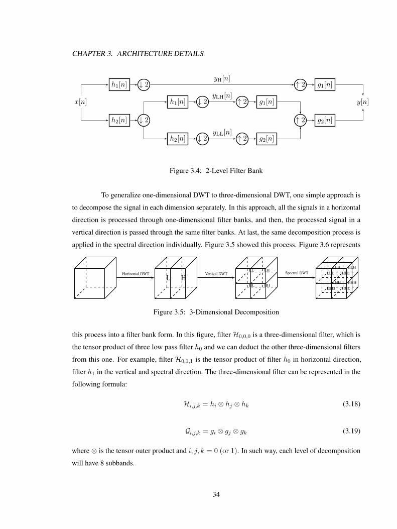
In Figure 3.4, a two levels of tree-structured filter banks is applied to a one-dimensional
signal x[n]. The signal x[n] is passed through a high-pass filter (HPF): h0[n] and a low-pass filter
(LPF): hL[n]. The HPF separates the high-frequency component yH [n] from original signal x[n],
and the LPF separates the low-frequency component yL[n] from signal x[n]. After downsampling by
2 in the highest frequency level, the high-frequency signal yH [n] is passed to the next module for
further operation. However, the coarse signal yL[n] is passed through the same filter banks again,
which are h0[n] and hL[n], to generate the high-frequency and low-frequency part of the signal
yL[n]. After downsampling, the 2-level decomposition of signal x[n] by DWT is finished and the
reconstruction part is just the inverted structure of the decomposition part.
33
CHAPTER 3. ARCHITECTURE DETAILS
x[n]
h2[n]
h1[n]
↓ 2
↓ 2
h1[n]
h2[n]
↓ 2
↓ 2
↑ 2
↑ 2
g1[n]
g2[n]
↑ 2 g2[n]
g1[n]↑ 2
y[n]yLH[n]
yLL[n]
yH[n]
Figure 3.4: 2-Level Filter Bank
To generalize one-dimensional DWT to three-dimensional DWT, one simple approach is
to decompose the signal in each dimension separately. In this approach, all the signals in a horizontal
direction is processed through one-dimensional filter banks, and then, the processed signal in a
vertical direction is passed through the same filter banks. At last, the same decomposition process is
applied in the spectral direction individually. Figure 3.5 showed this process. Figure 3.6 represents
L HLL LH
HL HH
LLL HLLHLH
LHLLHH
HLH HHLHHH
LLH
Vertical DWT Spectral DWTHorizontal DWT
Figure 3.5: 3-Dimensional Decomposition
this process into a filter bank form. In this figure, filterH0,0,0 is a three-dimensional filter, which is
the tensor product of three low pass filter h0 and we can deduct the other three-dimensional filters
from this one. For example, filter H0,1,1 is the tensor product of filter h0 in horizontal direction,
filter h1 in the vertical and spectral direction. The three-dimensional filter can be represented in the
following formula:
Hi,j,k = hi ⊗ hj ⊗ hk (3.18)
Gi,j,k = gi ⊗ gj ⊗ gk (3.19)
where ⊗ is the tensor outer product and i, j, k = 0 (or 1). In such way, each level of decomposition
will have 8 subbands.
34
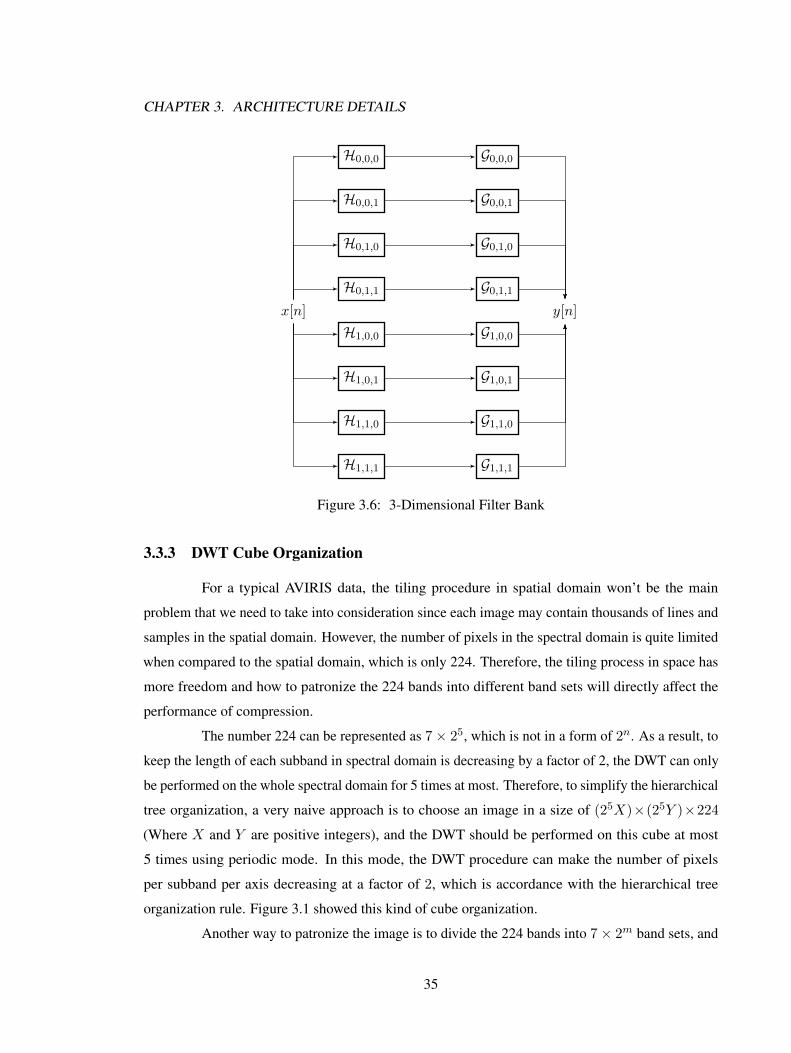
CHAPTER 3. ARCHITECTURE DETAILS
x[n]
H0,1,1
H1,0,0
H0,1,0
H0,0,1
H0,0,0
H1,0,1
H1,1,0
H1,1,1
G0,1,1
G1,0,0
G0,1,0
G0,0,1
G0,0,0
G1,0,1
G1,1,0
G1,1,1
y[n]
Figure 3.6: 3-Dimensional Filter Bank
3.3.3 DWT Cube Organization
For a typical AVIRIS data, the tiling procedure in spatial domain won’t be the main
problem that we need to take into consideration since each image may contain thousands of lines and
samples in the spatial domain. However, the number of pixels in the spectral domain is quite limited
when compared to the spatial domain, which is only 224. Therefore, the tiling process in space has
more freedom and how to patronize the 224 bands into different band sets will directly affect the
performance of compression.
The number 224 can be represented as 7× 25, which is not in a form of 2n. As a result, to
keep the length of each subband in spectral domain is decreasing by a factor of 2, the DWT can only
be performed on the whole spectral domain for 5 times at most. Therefore, to simplify the hierarchical
tree organization, a very naive approach is to choose an image in a size of (25X)×(25Y )×224(Where X and Y are positive integers), and the DWT should be performed on this cube at most
5 times using periodic mode. In this mode, the DWT procedure can make the number of pixels
per subband per axis decreasing at a factor of 2, which is accordance with the hierarchical tree
organization rule. Figure 3.1 showed this kind of cube organization.
Another way to patronize the image is to divide the 224 bands into 7× 2m band sets, and
35
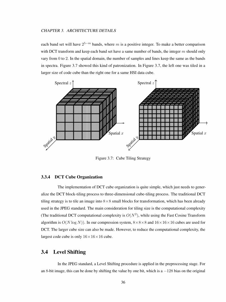
CHAPTER 3. ARCHITECTURE DETAILS
each band set will have 25−m bands, where m is a positive integer. To make a better comparison
with DCT transform and keep each band set have a same number of bands, the integer m should only
vary from 0 to 2. In the spatial domain, the number of samples and lines keep the same as the bands
in spectra. Figure 3.7 showed this kind of patronization. In Figure 3.7, the left one was tiled in a
larger size of code cube than the right one for a same HSI data cube.
Spatial x
Spectral z
Spatia
l ySpatial x
Spectral z
Spatia
l y
Figure 3.7: Cube Tiling Strategy
3.3.4 DCT Cube Organization
The implementation of DCT cube organization is quite simple, which just needs to gener-
alize the DCT block-tiling process to three-dimensional cube-tiling process. The traditional DCT
tiling strategy is to tile an image into 8×8 small blocks for transformation, which has been already
used in the JPEG standard. The main consideration for tiling size is the computational complexity
(The traditional DCT computational complexity is O(N2), while using the Fast Cosine Transform
algorithm is O(N logN)). In our compression system, 8×8×8 and 16×16×16 cubes are used for
DCT. The larger cube size can also be made. However, to reduce the computational complexity, the
largest code cube is only 16×16×16 cube.
3.4 Level Shifting
In the JPEG standard, a Level Shifting procedure is applied in the preprocessing stage. For
an 8-bit image, this can be done by shifting the value by one bit, which is a −128 bias on the original
36
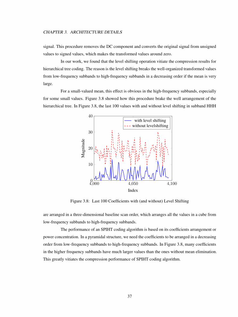
CHAPTER 3. ARCHITECTURE DETAILS
signal. This procedure removes the DC component and converts the original signal from unsigned
values to signed values, which makes the transformed values around zero.
In our work, we found that the level shifting operation vitiate the compression results for
hierarchical tree coding. The reason is the level shifting breaks the well-organized transformed values
from low-frequency subbands to high-frequency subbands in a decreasing order if the mean is very
large.
For a small-valued mean, this effect is obvious in the high-frequency subbands, especially
for some small values. Figure 3.8 showed how this procedure brake the well arrangement of the
hierarchical tree. In Figure 3.8, the last 100 values with and without level shifting in subband HHH
4,000 4,050 4,1000
10
20
30
40
Index
Mag
nitu
de
with level shiftingwithout levelshifting
Figure 3.8: Last 100 Coefficients with (and without) Level Shifting
are arranged in a three-dimensional baseline scan order, which arranges all the values in a cube from
low-frequency subbands to high-frequency subbands.
The performance of an SPIHT coding algorithm is based on its coefficients arrangement or
power concentration. In a pyramidal structure, we need the coefficients to be arranged in a decreasing
order from low-frequency subbands to high-frequency subbands. In Figure 3.8, many coefficients
in the higher frequency subbands have much larger values than the ones without mean elimination.
This greatly vitiates the compression performance of SPIHT coding algorithm.
37
CHAPTER 3. ARCHITECTURE DETAILS
3.5 Summary
In this chapter, we introduced the 3D-SPIHT algorithm from the pyramidal structure of
a transformed cube. After defining the hierarchical tree relationship between each coefficients,
the 3D-SPIHT process can be easily derived. The cube tilling rules are also introduced here. We
intentionally spared a section to discuss how the performance of the SPIHT algorithm is affected by
the arrangement of different coefficients. As a result, for a better compression ratio, we want the large
coefficients to be concentrated at the lower frequency bands amongst different subbands. We also
want the large coefficients can be concentrated as clusters in each subband. At last, we showed that
the level shifting process is not needed in our algorithm which is different from the JPEG standard.
38

CHAPTER 3. ARCHITECTURE DETAILS
Algorithm 1 Dominant Pass1: while T > Tc do
2: T = T/2
3: for every cx,y,z ∈ LIP do
4: output sgn(cx,y,z)
5: if J(cx,y,z) 6= 0 then
6: LSP← cx,y,z
7: end if
8: end for
9: for every cx,y,z ∈ LIS do
10: if cx,y,z is type A then
11: Output J(O(cx,y,z))
12: if J(O(cx,y,z)) 6= 0 then
13: for every cx,y,z ∈ C(cx,y,z) do
14: Output sgn(cx,y,z)
15: if J(cx,y,z) 6= 0 then
16: LSP← cx,y,z
17: else
18: LIP← cx,y,z
19: end if
20: end for
21: if G(cx,y,z) 6= ∅ then
22: set cx,y,z as type B, move cx,y,z to then end of LIP
23: else
24: remove cx,y,z from LIS
25: end if
26: end if
27: else
28: Output J(G(cx,y,z))
29: if J(G(cx,y,z)) ==1 then
30: LIS← C(cx,y,z))31: Delete cx,y,z from LIS
32: end if
33: end if
34: end for
35: end while
39

CHAPTER 3. ARCHITECTURE DETAILS
Algorithm 2 Subordinate Pass1: for every cx,y,z ∈ LSP do
2: Quantizer← cx,y,z
3: Output quantized value: Q
4: end for
40
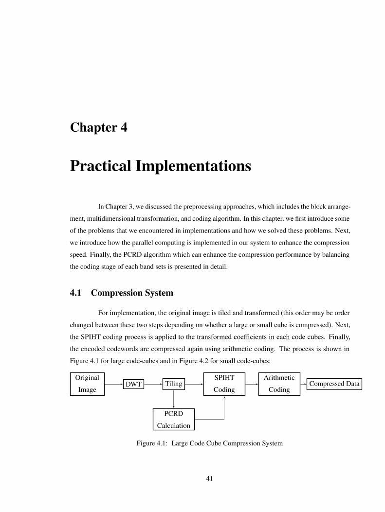
Chapter 4
Practical Implementations
In Chapter 3, we discussed the preprocessing approaches, which includes the block arrange-
ment, multidimensional transformation, and coding algorithm. In this chapter, we first introduce some
of the problems that we encountered in implementations and how we solved these problems. Next,
we introduce how the parallel computing is implemented in our system to enhance the compression
speed. Finally, the PCRD algorithm which can enhance the compression performance by balancing
the coding stage of each band sets is presented in detail.
4.1 Compression System
For implementation, the original image is tiled and transformed (this order may be order
changed between these two steps depending on whether a large or small cube is compressed). Next,
the SPIHT coding process is applied to the transformed coefficients in each code cubes. Finally,
the encoded codewords are compressed again using arithmetic coding. The process is shown in
Figure 4.1 for large code-cubes and in Figure 4.2 for small code-cubes:
Original
ImageDWT Tiling
PCRD
Calculation
SPIHT
Coding
Arithmetic
CodingCompressed Data
Figure 4.1: Large Code Cube Compression System
41
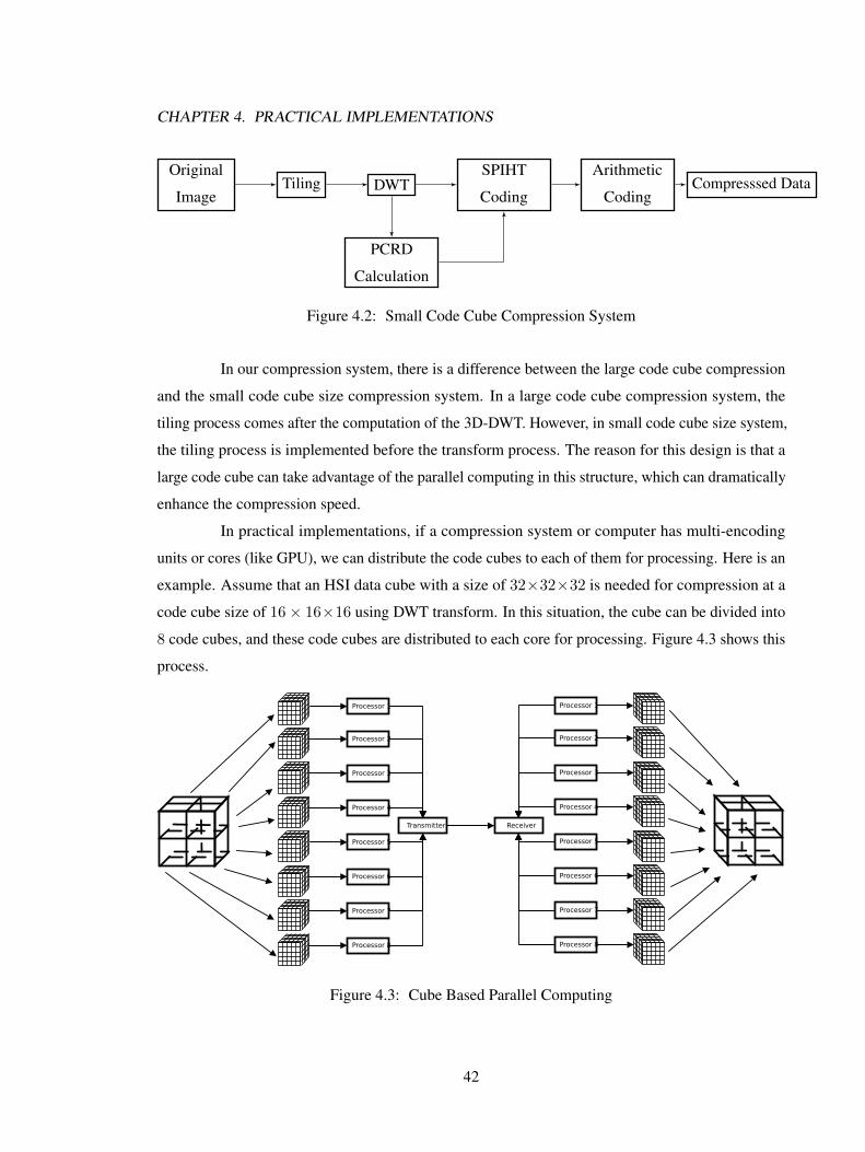
CHAPTER 4. PRACTICAL IMPLEMENTATIONS
Original
ImageTiling DWT
PCRD
Calculation
SPIHT
Coding
Arithmetic
CodingCompresssed Data
Figure 4.2: Small Code Cube Compression System
In our compression system, there is a difference between the large code cube compression
and the small code cube size compression system. In a large code cube compression system, the
tiling process comes after the computation of the 3D-DWT. However, in small code cube size system,
the tiling process is implemented before the transform process. The reason for this design is that a
large code cube can take advantage of the parallel computing in this structure, which can dramatically
enhance the compression speed.
In practical implementations, if a compression system or computer has multi-encoding
units or cores (like GPU), we can distribute the code cubes to each of them for processing. Here is an
example. Assume that an HSI data cube with a size of 32×32×32 is needed for compression at a
code cube size of 16× 16×16 using DWT transform. In this situation, the cube can be divided into
8 code cubes, and these code cubes are distributed to each core for processing. Figure 4.3 shows this
process.
Receiver
Processor 1
Transmitter
Processor 2
Processor 3
Processor 4
Processor 5
Processor 6
Processor 7
Processor 8
Processor 1
Processor 2
Processor 3
Processor 4
Processor 5
Processor 6
Processor 7
Processor 8
Figure 4.3: Cube Based Parallel Computing
42
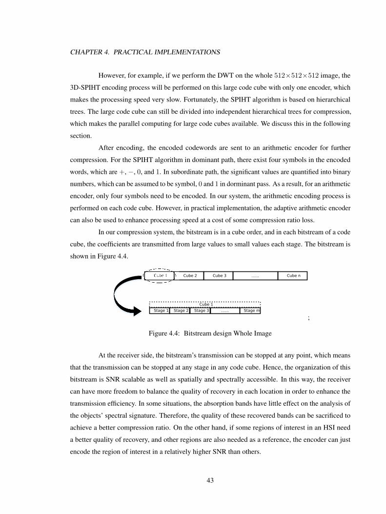
CHAPTER 4. PRACTICAL IMPLEMENTATIONS
However, for example, if we perform the DWT on the whole 512×512×512 image, the
3D-SPIHT encoding process will be performed on this large code cube with only one encoder, which
makes the processing speed very slow. Fortunately, the SPIHT algorithm is based on hierarchical
trees. The large code cube can still be divided into independent hierarchical trees for compression,
which makes the parallel computing for large code cubes available. We discuss this in the following
section.
After encoding, the encoded codewords are sent to an arithmetic encoder for further
compression. For the SPIHT algorithm in dominant path, there exist four symbols in the encoded
words, which are +, −, 0, and 1. In subordinate path, the significant values are quantified into binary
numbers, which can be assumed to be symbol, 0 and 1 in dorminant pass. As a result, for an arithmetic
encoder, only four symbols need to be encoded. In our system, the arithmetic encoding process is
performed on each code cube. However, in practical implementation, the adaptive arithmetic encoder
can also be used to enhance processing speed at a cost of some compression ratio loss.
In our compression system, the bitstream is in a cube order, and in each bitstream of a code
cube, the coefficients are transmitted from large values to small values each stage. The bitstream is
shown in Figure 4.4.
Cube 1 Cube 2 Cube 3 …… Cube n
Stage 1 Stage 2 Stage 3 …… Stage m
Cube 1
;
Figure 4.4: Bitstream design Whole Image
At the receiver side, the bitstream’s transmission can be stopped at any point, which means
that the transmission can be stopped at any stage in any code cube. Hence, the organization of this
bitstream is SNR scalable as well as spatially and spectrally accessible. In this way, the receiver
can have more freedom to balance the quality of recovery in each location in order to enhance the
transmission efficiency. In some situations, the absorption bands have little effect on the analysis of
the objects’ spectral signature. Therefore, the quality of these recovered bands can be sacrificed to
achieve a better compression ratio. On the other hand, if some regions of interest in an HSI need
a better quality of recovery, and other regions are also needed as a reference, the encoder can just
encode the region of interest in a relatively higher SNR than others.
43

CHAPTER 4. PRACTICAL IMPLEMENTATIONS
4.2 Post Compression Rate Distortion (PCRD) Algorithm
The PCRD algorithm is developed to optimize the Rate-Distortion ratio by choosing
the optimal cutting points. The mathematical model of this algorithm was firstly introduced by
Hugh Everett in his paper, who used a generalized Lagrange multiplier methods for solving this
problem [19].
For a simplified presentation, we ignore the size of each cube and their contributed
difference to the whole image. We denote, the code length of the whole image after compression
by L, and the length i for each cube by Li. As a result, the code length of the whole image can be
represented as:
L =∑i
Li (4.1)
In our algorithm, we can get different code lengths at different distortions since the SPIHT algorithm
is SNR scalable. If for some reasons, we want the whole image after compression to be less than
some values of length Lmax, then the code length of different cubes in the whole image should be
truncated at some truncation point ci. The code length of the image can now be represented as:
L =∑i
Lci,i ≤ Lmax (4.2)
where Lci,i is the coding length of ith block truncated at jth point ci,j .
The other factor that we need to take into consideration is distortion. At a compression
and coding stage, we assume that the transform is orthogonal. So that, the distortion can be directly
calculated from the difference between encoded transformed coefficients and the original ones.
In our system, it’s obvious that DCT is an orthogonal transform. Although some wavelets, for
example, bi-orthogonal wavelets CDF 9/7 and CDF 5/3 wavelets are not orthogonal wavelets,
the distortion still can be calculated approximately from the wavelet coefficients because of their
near-orthogonal feature. In our system’s division of cubes, the distortion is summable since all the
cubes are independent of each other. If we take the truncation points into consideration, the overall
distortion D can be represented as:
D =∑i
Dci,i (4.3)
where Dci,i is the distortion of ith block truncated at jth point ci,j .
44
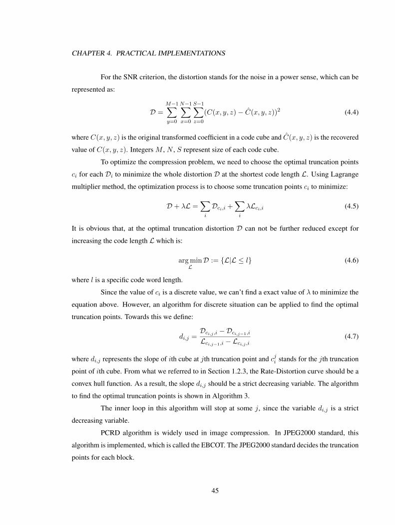
CHAPTER 4. PRACTICAL IMPLEMENTATIONS
For the SNR criterion, the distortion stands for the noise in a power sense, which can be
represented as:
D =M−1∑y=0
N−1∑x=0
S−1∑z=0
(C(x, y, z)− C(x, y, z))2 (4.4)
where C(x, y, z) is the original transformed coefficient in a code cube and C(x, y, z) is the recovered
value of C(x, y, z). Integers M , N , S represent size of each code cube.
To optimize the compression problem, we need to choose the optimal truncation points
ci for each Di to minimize the whole distortion D at the shortest code length L. Using Lagrange
multiplier method, the optimization process is to choose some truncation points ci to minimize:
D + λL =∑i
Dci,i +∑i
λLci,i (4.5)
It is obvious that, at the optimal truncation distortion D can not be further reduced except for
increasing the code length L which is:
argminL
D := {L|L ≤ l} (4.6)
where l is a specific code word length.
Since the value of ci is a discrete value, we can’t find a exact value of λ to minimize the
equation above. However, an algorithm for discrete situation can be applied to find the optimal
truncation points. Towards this we define:
di,j =Dci,j ,i −Dci,j−1,i
Lci,j−1,i − Lci,j ,i(4.7)
where di,j represents the slope of ith cube at jth truncation point and cji stands for the jth truncation
point of ith cube. From what we referred to in Section 1.2.3, the Rate-Distortion curve should be a
convex hull function. As a result, the slope di,j should be a strict decreasing variable. The algorithm
to find the optimal truncation points is shown in Algorithm 3.
The inner loop in this algorithm will stop at some j, since the variable di,j is a strict
decreasing variable.
PCRD algorithm is widely used in image compression. In JPEG2000 standard, this
algorithm is implemented, which is called the EBCOT. The JPEG2000 standard decides the truncation
points for each block.
45
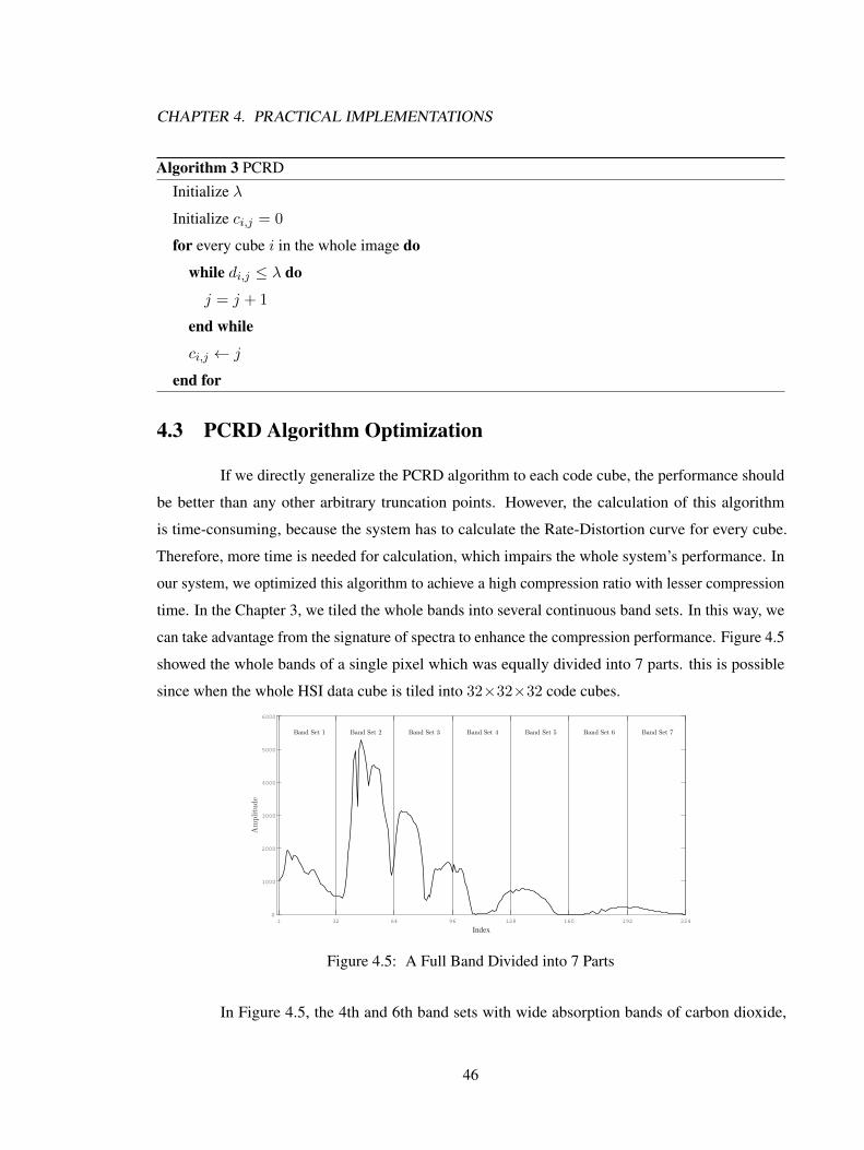
CHAPTER 4. PRACTICAL IMPLEMENTATIONS
Algorithm 3 PCRDInitialize λ
Initialize ci,j = 0
for every cube i in the whole image do
while di,j ≤ λ do
j = j + 1
end while
ci,j ← j
end for
4.3 PCRD Algorithm Optimization
If we directly generalize the PCRD algorithm to each code cube, the performance should
be better than any other arbitrary truncation points. However, the calculation of this algorithm
is time-consuming, because the system has to calculate the Rate-Distortion curve for every cube.
Therefore, more time is needed for calculation, which impairs the whole system’s performance. In
our system, we optimized this algorithm to achieve a high compression ratio with lesser compression
time. In the Chapter 3, we tiled the whole bands into several continuous band sets. In this way, we
can take advantage from the signature of spectra to enhance the compression performance. Figure 4.5
showed the whole bands of a single pixel which was equally divided into 7 parts. this is possible
since when the whole HSI data cube is tiled into 32×32×32 code cubes.
1 32 64 96 128 160 192 224
Index
0
1000
2000
3000
4000
5000
6000
Amplitude
Band Set 1 Band Set 2 Band Set 3 Band Set 4 Band Set 5 Band Set 6 Band Set 7
Figure 4.5: A Full Band Divided into 7 Parts
In Figure 4.5, the 4th and 6th band sets with wide absorption bands of carbon dioxide,
46
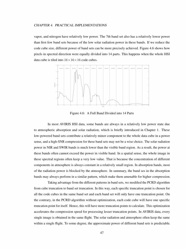
CHAPTER 4. PRACTICAL IMPLEMENTATIONS
vapor, and nitrogen have relatively low power. The 7th band set also has a relatively lower power
than first few band sets because of the low solar radiation power in these bands. If we reduce the
code cube size, different power of band sets can be more precisely achieved. Figure 4.6 shows how
pixels in spectral direction were equally divided into 14 parts. This happens when the whole HSI
data cube is tiled into 16×16×16 code cubes.
1 16 32 48 64 80 96 112 128 144 160 176 192 208 224
Index
0
1000
2000
3000
4000
5000
6000
Amplitude
Band Set 1 Band Set 2 Band Set 3 Band Set 4 Band Set 5 Band Set 6 Band Set 7 Band Set 8 Band Set 9 Band Set 10 Band Set 11 Band Set 12 Band Set 13 Band Set 14
Figure 4.6: A Full Band Divided into 14 Parts
In most AVIRIS HSI data, some bands are always in a relatively low power state due
to atmospheric absorption and solar radiation, which is briefly introduced in Chapter 1. These
low-powered band sets contribute a relatively minor component to the whole data cube in a power
sense, and a high-SNR compression for these band sets may not be a wise choice. The solar radiation
power in NIR and SWIR bands is much lower than the visible band region. As a result, the power at
these bands often cannot exceed the power in visible band. In a spatial sense, the whole image in
these spectral regions often keep a very low value. That is because the concentration of different
components in atmosphere is always constant in a relatively small region. In absorption bands, most
of the radiation power is blocked by the atmosphere. In summary, the band ses in the absorption
bands may always perform in a similar pattern, which make them amenable for higher compression.
Taking advantage from the different patterns in band sets, we modified the PCRD algorithm
from cube truncation to band set truncation. In this way, each specific truncation point is chosen for
all the code cubes in the same band set and each band set will only have one truncation point. On
the contrary, in the PCRD algorithm without optimization, each code cube will have one specific
truncation point for itself. Hence, this will have more truncation points to calculate. This optimization
accelerates the compression speed for processing lesser truncation points. In AVIRIS data, every
single image is obtained in the same flight. The solar radiation and atmosphere often keep the same
within a single flight. To some degree, the approximate power of different band sets is predictable.
47
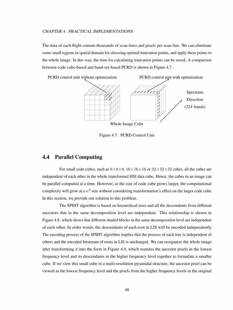
CHAPTER 4. PRACTICAL IMPLEMENTATIONS
The data of each flight contain thousands of scan-lines and pixels per scan line. We can eliminate
some small regions in spatial domain for choosing optimal truncation points, and apply these points to
the whole image. In this way, the time for calculating truncation points can be saved. A comparison
between code-cube-based and band-set-based PCRD is shown in Figure 4.7.
Spectrum
Direction
(224 bands)
PCRD control unit without optimization PCRD control unit with optimization
Whole Image Cube
Figure 4.7: PCRD Control Unit
4.4 Parallel Computing
For small code cubes, such as 8×8×8, 16×16×16 or 32×32×32 cubes, all the cubes are
independent of each other in the whole transformed HSI data cube. Hence, the cubes in an image can
be parallel computed at a time. However, as the size of code cube grows larger, the computational
complexity will grow at a n3 size without considering transformation’s effect on the larger code cube.
In this section, we provide our solution to this problem.
The SPIHT algorithm is based on hierarchical trees and all the descendants from different
ancestors that in the same decomposition level are independent. This relationship is shown in
Figure 4.8. which shows that different shaded blocks in the same decomposition level are independent
of each other. In order words, the descendants of each root in LIS will be encoded independently.
The encoding process of the SPIHT algorithm implies that the process of each tree is independent of
others and the encoded bitstream of roots in LIS is unchanged. We can reorganize the whole image
after transforming it into the form in Figure 4.9, which reunites the ancestor pixels in the lowest
frequency level and its descendants in the higher frequency level together to formulate a smaller
cube. If we view this small cube in a multi-resolution pyramidal structure, the ancestor pixel can be
viewed as the lowest frequency level and the pixels from the higher frequency levels in the original
48
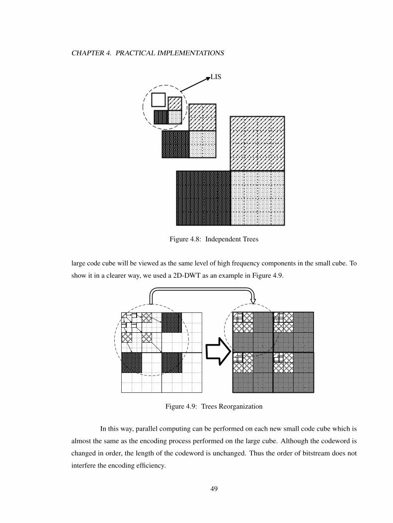
CHAPTER 4. PRACTICAL IMPLEMENTATIONS
LIS
Figure 4.8: Independent Trees
large code cube will be viewed as the same level of high frequency components in the small cube. To
show it in a clearer way, we used a 2D-DWT as an example in Figure 4.9.
Figure 4.9: Trees Reorganization
In this way, parallel computing can be performed on each new small code cube which is
almost the same as the encoding process performed on the large cube. Although the codeword is
changed in order, the length of the codeword is unchanged. Thus the order of bitstream does not
interfere the encoding efficiency.
49
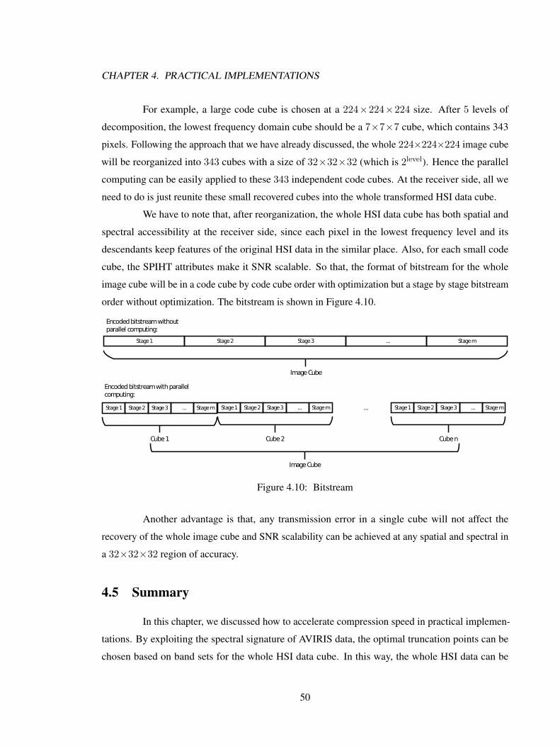
CHAPTER 4. PRACTICAL IMPLEMENTATIONS
For example, a large code cube is chosen at a 224×224×224 size. After 5 levels of
decomposition, the lowest frequency domain cube should be a 7×7×7 cube, which contains 343
pixels. Following the approach that we have already discussed, the whole 224×224×224 image cube
will be reorganized into 343 cubes with a size of 32×32×32 (which is 2level). Hence the parallel
computing can be easily applied to these 343 independent code cubes. At the receiver side, all we
need to do is just reunite these small recovered cubes into the whole transformed HSI data cube.
We have to note that, after reorganization, the whole HSI data cube has both spatial and
spectral accessibility at the receiver side, since each pixel in the lowest frequency level and its
descendants keep features of the original HSI data in the similar place. Also, for each small code
cube, the SPIHT attributes make it SNR scalable. So that, the format of bitstream for the whole
image cube will be in a code cube by code cube order with optimization but a stage by stage bitstream
order without optimization. The bitstream is shown in Figure 4.10.
Stage 1 Stage 2 Stage 3 ... Stage m
Stage 1 Stage 2 Stage 3 ... Stage m Stage 1 Stage 2 Stage 3 ... Stage m Stage 1 Stage 2 Stage 3 ... Stage m
Cube 1 Cube 2 Cube n
...
Encoded bitstream without parallel computing:
Encoded bitstream with parallel computing:
Image Cube
Image Cube
Figure 4.10: Bitstream
Another advantage is that, any transmission error in a single cube will not affect the
recovery of the whole image cube and SNR scalability can be achieved at any spatial and spectral in
a 32×32×32 region of accuracy.
4.5 Summary
In this chapter, we discussed how to accelerate compression speed in practical implemen-
tations. By exploiting the spectral signature of AVIRIS data, the optimal truncation points can be
chosen based on band sets for the whole HSI data cube. In this way, the whole HSI data can be
50

CHAPTER 4. PRACTICAL IMPLEMENTATIONS
compressed without calculating these truncation points which are decided from sample data. By
utilizing the independence of different hierarchical trees in DWT, a large transformed cube can
be decomposed into small code cubes for parallel encoding. The only difference is in the output
codeword order. However, the reorganization of the codeword order makes the recovery of the whole
HSI data cube spatial and spectral accessible and the transmission reliability is enhanced by this
approach.
51
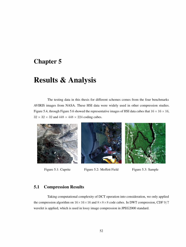
Chapter 5
Results & Analysis
The testing data in this thesis for different schemes comes from the four benchmarks
AVIRIS images from NASA. These HSI data were widely used in other compression studies.
Figure 5.4, through Figure 5.6 showed the representative images of HSI data cubes that 16× 16× 16,
32× 32× 32 and 448× 448× 224 coding cubes.
Figure 5.1: Cuprite Figure 5.2: Moffett Field Figure 5.3: Sample
5.1 Compression Results
Taking computational complexity of DCT operation into consideration, we only applied
the compression algorithm on 16×16×16 and 8×8×8 code cubes. In DWT compression, CDF 9/7
wavelet is applied, which is used in lossy image compression in JPEG2000 standard.
52
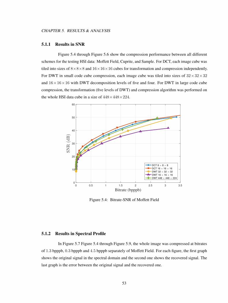
CHAPTER 5. RESULTS & ANALYSIS
5.1.1 Results in SNR
Figure 5.4 through Figure 5.6 show the compression performance between all different
schemes for the testing HSI data: Moffett Field, Cuprite, and Sample. For DCT, each image cube was
tiled into sizes of 8×8×8 and 16×16×16 cubes for transformation and compression independently.
For DWT in small code cube compression, each image cube was tiled into sizes of 32×32×32
and 16×16×16 with DWT decomposition levels of five and four. For DWT in large code cube
compression, the transformation (five levels of DWT) and compression algorithm was performed on
the whole HSI data cube in a size of 448×448×224.
0 0.5 1 1.5 2 2.5 3 3.5
Bitrate (bpppb)
0
10
20
30
40
50
60
SNR
(dB)
DCT 8 × 8 × 8
DCT 16 × 16 × 16
DWT 32 × 32 × 32
DWT 16 × 16 × 16
DWT 448 × 448 × 224
Figure 5.4: Bitrate-SNR of Moffett Field
5.1.2 Results in Spectral Profile
In Figure 5.7 Figure 5.4 through Figure 5.9, the whole image was compressed at bitrates
of 1.3 bpppb, 0.3 bpppb and 4.5 bpppb separately of Moffett Field. For each figure, the first graph
shows the original signal in the spectral domain and the second one shows the recovered signal. The
last graph is the error between the original signal and the recovered one.
53
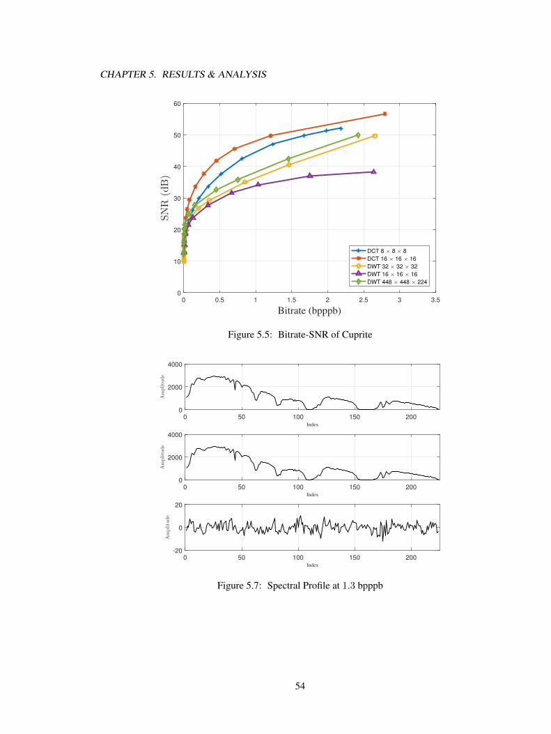
CHAPTER 5. RESULTS & ANALYSIS
0 0.5 1 1.5 2 2.5 3 3.5
Bitrate (bpppb)
0
10
20
30
40
50
60
SNR
(dB)
DCT 8 × 8 × 8
DCT 16 × 16 × 16
DWT 32 × 32 × 32
DWT 16 × 16 × 16
DWT 448 × 448 × 224
Figure 5.5: Bitrate-SNR of Cuprite
0 50 100 150 200
Index
0
2000
4000
Amplitude
0 50 100 150 200
Index
0
2000
4000
Amplitude
0 50 100 150 200
Index
-20
0
20
Amplitude
Figure 5.7: Spectral Profile at 1.3 bpppb
54
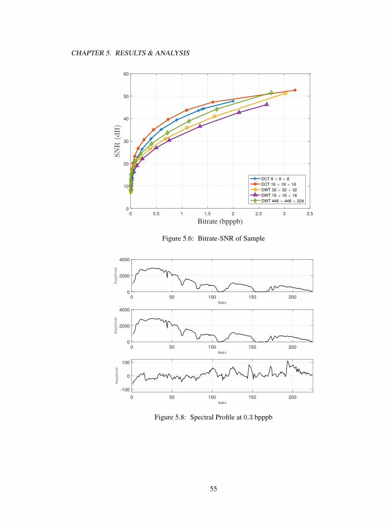
CHAPTER 5. RESULTS & ANALYSIS
0 0.5 1 1.5 2 2.5 3 3.5
Bitrate (bpppb)
0
10
20
30
40
50
60
SNR
(dB)
DCT 8 × 8 × 8
DCT 16 × 16 × 16
DWT 32 × 32 × 32
DWT 16 × 16 × 16
DWT 448 × 448 × 224
Figure 5.6: Bitrate-SNR of Sample
0 50 100 150 200
Index
0
2000
4000
Amplitude
0 50 100 150 200
Index
0
2000
4000
Amplitude
0 50 100 150 200
Index
-100
0
100
Amplitude
Figure 5.8: Spectral Profile at 0.3 bpppb
55
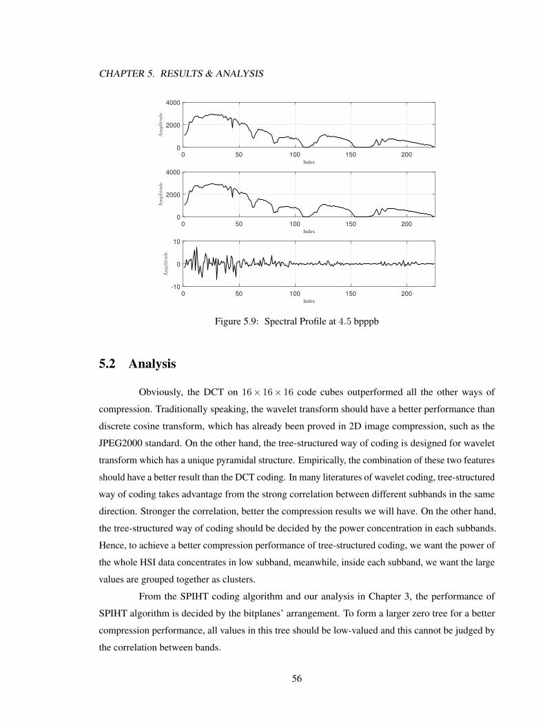
CHAPTER 5. RESULTS & ANALYSIS
0 50 100 150 200
Index
0
2000
4000
Amplitude
0 50 100 150 200
Index
0
2000
4000
Amplitude
0 50 100 150 200
Index
-10
0
10
Amplitude
Figure 5.9: Spectral Profile at 4.5 bpppb
5.2 Analysis
Obviously, the DCT on 16× 16× 16 code cubes outperformed all the other ways of
compression. Traditionally speaking, the wavelet transform should have a better performance than
discrete cosine transform, which has already been proved in 2D image compression, such as the
JPEG2000 standard. On the other hand, the tree-structured way of coding is designed for wavelet
transform which has a unique pyramidal structure. Empirically, the combination of these two features
should have a better result than the DCT coding. In many literatures of wavelet coding, tree-structured
way of coding takes advantage from the strong correlation between different subbands in the same
direction. Stronger the correlation, better the compression results we will have. On the other hand,
the tree-structured way of coding should be decided by the power concentration in each subbands.
Hence, to achieve a better compression performance of tree-structured coding, we want the power of
the whole HSI data concentrates in low subband, meanwhile, inside each subband, we want the large
values are grouped together as clusters.
From the SPIHT coding algorithm and our analysis in Chapter 3, the performance of
SPIHT algorithm is decided by the bitplanes’ arrangement. To form a larger zero tree for a better
compression performance, all values in this tree should be low-valued and this cannot be judged by
the correlation between bands.
56
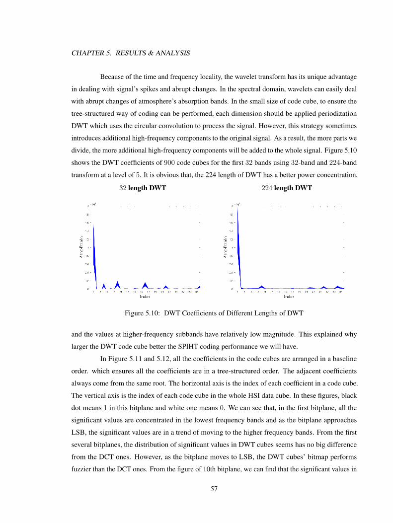
CHAPTER 5. RESULTS & ANALYSIS
Because of the time and frequency locality, the wavelet transform has its unique advantage
in dealing with signal’s spikes and abrupt changes. In the spectral domain, wavelets can easily deal
with abrupt changes of atmosphere’s absorption bands. In the small size of code cube, to ensure the
tree-structured way of coding can be performed, each dimension should be applied periodization
DWT which uses the circular convolution to process the signal. However, this strategy sometimes
introduces additional high-frequency components to the original signal. As a result, the more parts we
divide, the more additional high-frequency components will be added to the whole signal. Figure 5.10
shows the DWT coefficients of 900 code cubes for the first 32 bands using 32-band and 224-band
transform at a level of 5. It is obvious that, the 224 length of DWT has a better power concentration,
32 length DWT 224 length DWT
Figure 5.10: DWT Coefficients of Different Lengths of DWT
and the values at higher-frequency subbands have relatively low magnitude. This explained why
larger the DWT code cube better the SPIHT coding performance we will have.
In Figure 5.11 and 5.12, all the coefficients in the code cubes are arranged in a baseline
order. which ensures all the coefficients are in a tree-structured order. The adjacent coefficients
always come from the same root. The horizontal axis is the index of each coefficient in a code cube.
The vertical axis is the index of each code cube in the whole HSI data cube. In these figures, black
dot means 1 in this bitplane and white one means 0. We can see that, in the first bitplane, all the
significant values are concentrated in the lowest frequency bands and as the bitplane approaches
LSB, the significant values are in a trend of moving to the higher frequency bands. From the first
several bitplanes, the distribution of significant values in DWT cubes seems has no big difference
from the DCT ones. However, as the bitplane moves to LSB, the DWT cubes’ bitmap performs
fuzzier than the DCT ones. From the figure of 10th bitplane, we can find that the significant values in
57
CHAPTER 5. RESULTS & ANALYSIS
10th bitplane always appear in some specific positions in most of the cubes. On the contrary, the
DWT cubes’ significant values distribute in a wider range.
The situation becomes the worst in the 13th bitplane. The DWT cubes’ bitplane becomes
fuzzier and we can see several dark lines after 2000 samples, which belong to the highest frequency
bands. From what we have discussed in the former chapter, large values in highest frequency
subbands significantly vitiates the efficiency of the SPIHT algorithm, and almost all the code cubes
in this whole HSI data cube have this deficiency. Compared to the DWT cubes, the DCT cubes seem
didn’t change much from the 10th bitplane, only some bits are significant in the highest frequency
subbands and this explained why DCT based algorithm has a better performance.
5.3 Summary
In this chapter, we applied DWT and DCT to three different HSI data cubes. Taking the
computational complexity into consideration, we only perform DCT on 8×8×8 and 16×16×16 code
cubes. From the results, we conclude that, the DCT based 3D-SPIHT algorithm with a 16×16×16code cube size achieves the best compression ratio under given SNR. From the bitplane map of
DCT and DWT coefficients in the same HSI data cube, the DWT based code cubes’ bitplane map
is fuzzier than the DCT ones, especially when the bitplane goes toward LSB, though there are no
big difference in the first several bitplanes. This is in accordance with the conclusion we made in
Chapter 3 and this phenomenon also implies why the difference of compression results between
these two transformations are not very big when the bitrate is very low. Hence, although the SPIHT
algorithm is designed for DWT, in some specific situations (regarding cube size) the SPIHT algorithm
with DCT still can have a competitive performance. DCT does not have the pyramidal structure in
DWT, however, in some situations, its bitplanes’ arrangement is more suitable for SPIHT algorithm.
58
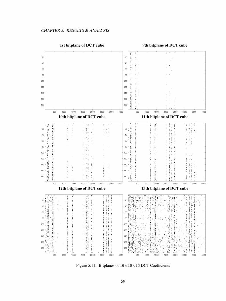
CHAPTER 5. RESULTS & ANALYSIS
1st bitplane of DCT cube
500 1000 1500 2000 2500 3000 3500 4000
20
40
60
80
100
120
140
160
180
9th bitplane of DCT cube
500 1000 1500 2000 2500 3000 3500 4000
20
40
60
80
100
120
140
160
180
10th bitplane of DCT cube
500 1000 1500 2000 2500 3000 3500 4000
20
40
60
80
100
120
140
160
180
11th bitplane of DCT cube
500 1000 1500 2000 2500 3000 3500 4000
20
40
60
80
100
120
140
160
180
12th bitplane of DCT cube
500 1000 1500 2000 2500 3000 3500 4000
20
40
60
80
100
120
140
160
180
13th bitplane of DCT cube
500 1000 1500 2000 2500 3000 3500 4000
20
40
60
80
100
120
140
160
180
Figure 5.11: Bitplanes of 16×16×16 DCT Coefficients
59
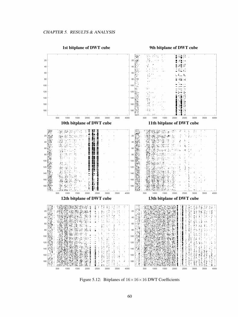
CHAPTER 5. RESULTS & ANALYSIS
1st bitplane of DWT cube
500 1000 1500 2000 2500 3000 3500 4000
20
40
60
80
100
120
140
160
180
9th bitplane of DWT cube
500 1000 1500 2000 2500 3000 3500 4000
20
40
60
80
100
120
140
160
180
10th bitplane of DWT cube
500 1000 1500 2000 2500 3000 3500 4000
20
40
60
80
100
120
140
160
180
11th bitplane of DWT cube
500 1000 1500 2000 2500 3000 3500 4000
20
40
60
80
100
120
140
160
180
12th bitplane of DWT cube
500 1000 1500 2000 2500 3000 3500 4000
20
40
60
80
100
120
140
160
180
13th bitplane of DWT cube
500 1000 1500 2000 2500 3000 3500 4000
20
40
60
80
100
120
140
160
180
Figure 5.12: Bitplanes of 16×16×16 DWT Coefficients
60
Chapter 6
Conclusions and Future Work
6.1 Conclusion
Lossy HSI data compression significantly helps in HSI data storage and transmission.
By discarding some information of the original data under an acceptable range, HSI data can be
compressed to a very small size. In this thesis, we presented a novel architecture for compressing
AVIRIS data with pre-processing and compression stage. In our test, we showed that this system
is proved to be effective in compressing HSI data. In the compression stage, we take practical
implementations into consideration. In this stage, we modified the PCRD algorithm in AVIRIS
data compression and implemented parallel computing. These modifications make the compression
system more efficient. From previous works in HSI data compression using DWT, the approaches
are often the combination of three-dimensional DWT and wavelet coding algorithm (such as SPIHT,
EZW or SPECK). However, we focused on the traditional DCT in our work, and combined this
transformation with the wavelet coding algorithm. The results is better than the traditional DWT. In
our system, the 3D-SPIHT coding algorithm is applied and results that can predict the performance
of SPIHT coding theoretically are also derived. These conclusions helped us analyze compression
results.
In the compression stage, the system’s performance is enhanced by implementing parallel
computing and the modified PCRD algorithm. In parallel computing, taking advantage from the
independence of hierarchical trees, the large code cube can be decomposed into independent small
code cubes for compression. As a result, the spatial and spectral accessibility can be both achieved.
For reducing the computational complexity in the PCRD algorithm, we modified the the PCRD
process from code cube based to band set based. Taking advantage from the features in spectra of
61
CHAPTER 6. CONCLUSIONS AND FUTURE WORK
AVIRIS data, the times of PCRD procedure to be performed can be highly reduced.
Finally, we gave our results in different cube sizes of compression. We found that, larger
the code cube, better the compression results will be for the DWT coding. However, the 16× 16× 16
size of code cube while using DCT outperformed all the others. We analyzed our results using
bitplanes and the results were compatible with our theoretical conclusion.
6.2 Future Work
In this thesis, we applied cosine signal and CDF 9/7 wavelet as our basis for decomposition.
It has already been proved that, the discrete cosine basis are the suboptimal basis for decomposing
natural images. However, for hyperspectral images, the image from a single band is fuzzier than the
common images and as the spectral dimension is added in, the situation becomes complex. Hence,
the future work can focus on finding some optimal or suboptimal basis for hyperspectral image
compression.
Most works concerning the transform coding for hyperspectral images used transformation
to each dimension independently. To deal with the multi-dimensional decomposition, tensor is
an option for this problem. However, with the computational complexity and the freedom of
decomposition, we don’t know whether this way is applicable in practical. Hence the future work
can focus on whether tensor can be applied in practical use in hyperspectral image compression.
62
Bibliography
[1] N. J. P. Laboratory, “Spectra,” http://http://aviris.jpl.nasa.gov/aviris/spectrum.html.
[2] ——, “Airs,” http://http://http://airs.jpl.nasa.gov/mission and instrument/overview.
[3] G. Motta, F. Rizzo, and J. A. Storer, Hyperspectral data compression. Springer Science &
Business Media, 2006.
[4] C. E. Shannon, “A mathematical theory of communication,” ACM SIGMOBILE Mobile Com-
puting and Communications Review, vol. 5, no. 1, pp. 3–55, 2001.
[5] S. Golomb, “Run-length encodings (corresp.),” IEEE Transactions on Information Theory,
vol. 12, no. 3, pp. 399–401, Jul 1966.
[6] D. A. Huffman et al., “A method for the construction of minimum-redundancy codes,” Proceed-
ings of the IRE, vol. 40, no. 9, pp. 1098–1101, 1952.
[7] G. N. N. Martin, G. G. Langdon Jr, and S. J. Todd, “Arithmetic codes for constrained channels,”
IBM Journal of Research and Development, vol. 27, no. 2, pp. 94–106, 1983.
[8] G. Motta, F. Rizzo, and J. Storer, “Locally optimal partitioned vector quantization of hyper-
spectral data,” in Hyperspectral Data Compression. Springer, 2006, pp. 107–146.
[9] J. W. Schwartz and R. C. Barker, “Bit-plane encoding: a technique for source encoding,”
Aerospace and Electronic Systems, IEEE Transactions on, no. 4, pp. 385–392, 1966.
[10] R. C. Gonzalez and R. E. Woods, “Digital image processing,” 2002.
[11] W. Ray and R. Driver, “Further decomposition of the karhunen-loeve series representation of
a stationary random process,” IEEE Transactions on Information Theory, vol. 16, no. 6, pp.
663–668, 1970.
63
BIBLIOGRAPHY
[12] I. Daubechies et al., Ten lectures on wavelets. SIAM, 1992, vol. 61.
[13] D. G. Manolakis, V. K. Ingle, and S. M. Kogon, Statistical and adaptive signal processing:
spectral estimation, signal modeling, adaptive filtering, and array processing. Artech House
Norwood, 2005, vol. 46.
[14] J. M. Shapiro, “Embedded image coding using zerotrees of wavelet coefficients,” Signal
Processing, IEEE Transactions on, vol. 41, no. 12, pp. 3445–3462, 1993.
[15] A. Said and W. A. Pearlman, “A new, fast, and efficient image codec based on set partitioning
in hierarchical trees,” Circuits and Systems for Video Technology, IEEE Transactions on, vol. 6,
no. 3, pp. 243–250, 1996.
[16] D. Taubman, “High performance scalable image compression with ebcot,” Image Processing,
IEEE transactions on, vol. 9, no. 7, pp. 1158–1170, 2000.
[17] D. Taubman and M. Marcellin, JPEG2000 Image Compression Fundamentals, Standards and
Practice: Image Compression Fundamentals, Standards and Practice. Springer Science &
Business Media, 2012, vol. 642.
[18] X. Tang and W. A. Pearlman, “Three-dimensional wavelet-based compression of hyperspectral
images,” in Hyperspectral Data Compression. Springer, 2006, pp. 273–308.
[19] H. Everett III, “Generalized lagrange multiplier method for solving problems of optimum
allocation of resources,” Operations research, vol. 11, no. 3, pp. 399–417, 1963.
64
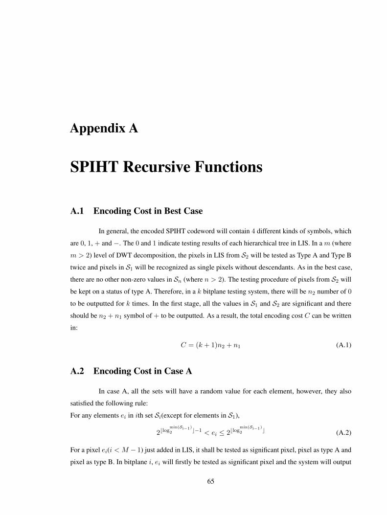
Appendix A
SPIHT Recursive Functions
A.1 Encoding Cost in Best Case
In general, the encoded SPIHT codeword will contain 4 different kinds of symbols, which
are 0, 1, + and −. The 0 and 1 indicate testing results of each hierarchical tree in LIS. In a m (where
m > 2) level of DWT decomposition, the pixels in LIS from S2 will be tested as Type A and Type B
twice and pixels in S1 will be recognized as single pixels without descendants. As in the best case,
there are no other non-zero values in Sn (where n > 2). The testing procedure of pixels from S2 will
be kept on a status of type A. Therefore, in a k bitplane testing system, there will be n2 number of 0
to be outputted for k times. In the first stage, all the values in S1 and S2 are significant and there
should be n2 + n1 symbol of + to be outputted. As a result, the total encoding cost C can be written
in:
C = (k + 1)n2 + n1 (A.1)
A.2 Encoding Cost in Case A
In case A, all the sets will have a random value for each element, however, they also
satisfied the following rule:
For any elements ei in ith set Si(except for elements in S1),
2blogmin(Si−1)
2 c−1 < ei ≤ 2blogmin(Si−1)
2 c (A.2)
For a pixel ei(i < M − 1) just added in LIS, it shall be tested as significant pixel, pixel as type A and
pixel as type B. In bitplane i, ei will firstly be tested as significant pixel and the system will output
65
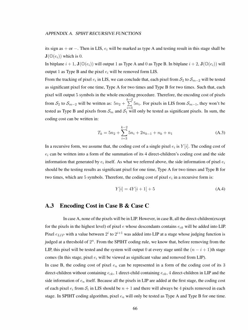
APPENDIX A. SPIHT RECURSIVE FUNCTIONS
its sign as + or −. Then in LIS, ei will be marked as type A and testing result in this stage shall be
J(O(ei)) which is 0.
In bitplane i+ 1, J(O(ei)) will output 1 as Type A and 0 as Type B. In bitplane i+ 2, J(O(ei)) will
output 1 as Type B and the pixel ei will be removed form LIS.
From the tracking of pixel ei in LIS, we can conclude that, each pixel from S2 to Sm−2 will be tested
as significant pixel for one time, Type A for two times and Type B for two times. Such that, each
pixel will output 5 symbols in the whole encoding procedure. Therefore, the encoding cost of pixels
from S2 to Sm−2 will be written as: 5n2 +k−2∑i=3
5ni. For pixels in LIS from Sm−1, they won’t be
tested as Type B and pixels from Sm and S1 will only be tested as significant pixels. In sum, the
coding cost can be written in:
Tk = 5n2 +k−2∑i=3
5ni + 2nk−1 + nk + n1 (A.3)
In a recursive form, we assume that, the coding cost of a single pixel ei is Y [i]. The coding cost of
ei can be written into a form of the summation of its 4 direct-children’s coding cost and the side
information that generated by ei itself. As what we referred above, the side information of pixel ei
should be the testing results as significant pixel for one time, Type A for two times and Type B for
two times, which are 5 symbols. Therefore, the coding cost of pixel ei in a recursive form is:
Y [i] = 4Y [i+ 1] + 5 (A.4)
A.3 Encoding Cost in Case B & Case C
In case A, none of the pixels will be in LIP. However, in case B, all the direct-children(except
for the pixels in the highest level) of pixel e whose descendants contains eck will be added into LIP.
Pixel eLIP with a value between 2i to 2i+1 was added into LIP at a stage whose judging function is
judged at a threshold of 2n. From the SPIHT coding rule, we know that, before removing from the
LIP, this pixel will be tested and the system will output 0 at every stage until the (n− i+ 1)th stage
comes (In this stage, pixel ei will be viewed as significant value and removed from LIP).
In case B, the coding cost of pixel en can be represented in a form of the coding cost of its 3
direct-children without containing eck, 1 direct-child containing eck, 4 direct-children in LIP and the
side information of en itself. Because all the pixels in LIP are added at the first stage, the coding cost
of each pixel ei from Si in LIS should be n+ 1 and there will always be 4 pixels removed in each
stage. In SPIHT coding algorithm, pixel en will only be tested as Type A and Type B for one time.
66
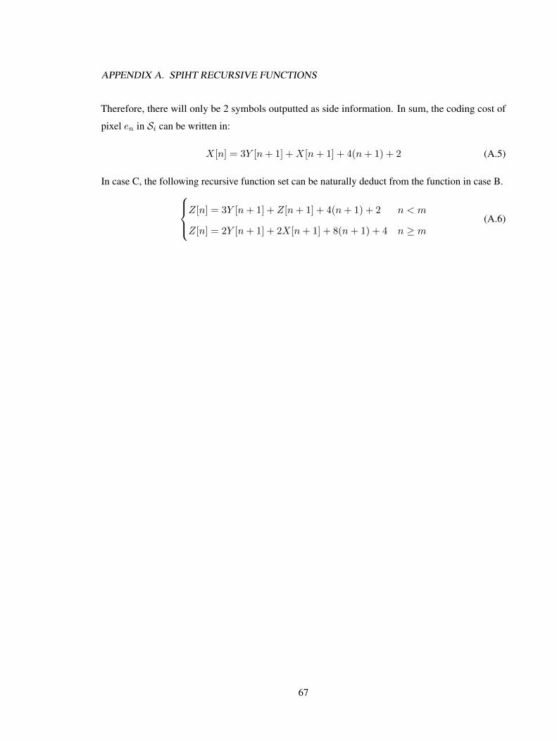
APPENDIX A. SPIHT RECURSIVE FUNCTIONS
Therefore, there will only be 2 symbols outputted as side information. In sum, the coding cost of
pixel en in Si can be written in:
X[n] = 3Y [n+ 1] +X[n+ 1] + 4(n+ 1) + 2 (A.5)
In case C, the following recursive function set can be naturally deduct from the function in case B.Z[n] = 3Y [n+ 1] + Z[n+ 1] + 4(n+ 1) + 2 n < m
Z[n] = 2Y [n+ 1] + 2X[n+ 1] + 8(n+ 1) + 4 n ≥ m(A.6)
67


![Fully Spatial and SNR Scalable, SPIHT-Based Image Coding ... · development of EZW, called Set Partitioning in Hierarchical Trees (SPIHT) algorithm by Said and Pearlman [7] is one](https://static.fdocuments.in/doc/165x107/5f44529edb9b345841711e49/fully-spatial-and-snr-scalable-spiht-based-image-coding-development-of-ezw.jpg)
![Matlab SPIHT[1]](https://static.fdocuments.in/doc/165x107/5536c21e5503463f7c8b4a65/matlab-spiht1.jpg)
![HYPERSPECTRAL IMAGE COMPRESSION USING …rdmodernresearch.org/wp-content/uploads/2015/12/114.pdfThe AT 3D SPIHT algorithm for hyper spectral image is proposed in [18]. In this algorithm,](https://static.fdocuments.in/doc/165x107/5ae88a917f8b9acc269045c7/hyperspectral-image-compression-using-at-3d-spiht-algorithm-for-hyper-spectral.jpg)