Aalborg UniversityInstitute of Energy TechnologyPower Electronics and Drives

DC Link Voltage Control

PED10-1013a

Institute of Energy Technology Aalborg University PED10 Spring

2008

Pontoppidanstræde 101 9220 Aalborg

TITLE: DC Link Voltage Control

THEME: PED 10th Master Project

PROJECT PERIOD: 4. February- 4. June 2008

PROJECT GROUP: PED10-1013a

Author:

Stefan Partyka

Supervisors:

Stig Munk-Nielsen, Associate Professor, AAU

Mads Krogsgaard, Sauer-Danfoss

No. of copies:3

No. of pages:94

Completed: 4. June 2008

The project purpose is to control an In-terior Permanent Magnet SynchronousGenerator in the way that DC linkvoltage is kept constant within +/- 10%limits, regardless of the applied loadand rotor speed.The converter topology selection wasperformed and the PWM rectifier topo-logy was selected for further investiga-tion. Then several methods of the fieldoriented control methods for generatorwere presented and at the end ConstantTorque Angle Control (CTAC) methodwas selected for further studies.The simulations of the generator sys-tem were made. The selected controlmethod was evaluated and verified. Thereliability of the control method isproven also.The selected control strategy was im-plemented in DSP then. Implementa-tion platform is also described.However due to time constraints in theproject work, implementation is done inperiod between project submissiondeadline – June 4th and final examdate, June 19th.

Preface

The presented report is the documentation of my project work in field of the Electrical Engineering,

specialization Power Electronics and Drives performed at the Aalborg University. Institute of Energy

Technology.

I would like to acknowledge Associate Professor, Stig Munk-Nielsen for supervising my project, valu-

able advices and patience during my project work. I would like also acknowledge Mads Krogsgaard

from Sauer Danfoss for given important clues regarding my project.

I would give special thanks to Szymon Beczkowski for crucial hints during the laboratory work and

and supportive advices for writing of the report.

Finally I would like give also special thanks to Torben Matzen for help in laboratory work.

The references to the literature used in the project are in [ ] brackets.

Acronyms used in the report may be found in the list of acronyms. A list of the nomenclature used in

the report can be found in the list of nomenclature. In the back of this report, a CD-ROM is attached.

Aalborg University, 4 June 2008

Stefan E. Partyka

Table of Contents

Chapter 1. Preliminaries........................................................................................................................................1

1.1. Introduction................................................................................................................................................1

1.2. Problem Analysis.......................................................................................................................................1

1.2.1. Generator with six-pulse diode rectifier........................................................................................2

1.2.2. Generator with boost type chopper converter..............................................................................2

1.2.3. Generator with boost PWM rectifier..............................................................................................3

1.3. Control Method..........................................................................................................................................4

1.3.1. Constant Torque Angle Control (CTAC).......................................................................................6

1.3.2. Maximum Torque per Ampere Control.........................................................................................7

1.3.3. Unity Power Factor Control.............................................................................................................8

1.4.Comparison and Selection of the Described Control Methods............................................................9

1.4.1. Analysis .............................................................................................................................................9

1.4.2. The Method Selection.....................................................................................................................10

1.5. Scope on the Project.................................................................................................................................10

1.6. Objective....................................................................................................................................................10

1.7. Resources and Tools.................................................................................................................................11

1.7.1 Resources...........................................................................................................................................11

1.7.2. Tools..................................................................................................................................................12

1.8. Initial problem..........................................................................................................................................12

1.9. The Structure of the Project.....................................................................................................................12

Chapter 2. Modelling...........................................................................................................................................15

2.1 Modelling...................................................................................................................................................15

2.1.1. Permanent Magnet Machine Model.............................................................................................15

2.1.2. DC Link Model................................................................................................................................18

2.1.3. Converter Model.............................................................................................................................18

2.1.4. Modulation Scheme........................................................................................................................20

2.2. Summary...................................................................................................................................................24

Chapter 3. Control System..................................................................................................................................26

3.1. Field Oriented Control of the Generator...............................................................................................26

3.2. Field Oriented Control.............................................................................................................................27

3.2.1. Field Oriented Control for Base Speed.........................................................................................27

3.2.2. Flux weakening mode....................................................................................................................28

3.3. Design of the Control System.................................................................................................................32

3.3.1. Design of the q axis controllers ....................................................................................................32

3.3.2. Design of the d-axis controllers.....................................................................................................47

3.4. Summary...................................................................................................................................................54

Chapter 4. Simulations Results and Implementation....................................................................................56

4.1. Simulations................................................................................................................................................56

4.1.1. Method of Testing............................................................................................................................56

4.1.2. Obtained Results..............................................................................................................................57

4.1.3. Model verification............................................................................................................................61

4.1.4. Summary...........................................................................................................................................61

4.2. Implementation........................................................................................................................................61

4.2.1. Digital Signal Processor...................................................................................................................61

4.2.2. Signal Sensing...................................................................................................................................63

4.2.3. Laboratory Set-up Layout...............................................................................................................64

4.3. Summary...................................................................................................................................................66

Chapter 5. Conclusions and Future Work........................................................................................................69

5.1. Conlcusions...............................................................................................................................................69

5.2. Future Work..............................................................................................................................................69

Acronyms..............................................................................................................................................................72

Nomenclature List................................................................................................................................................75

Bibliography..........................................................................................................................................................78

Appendix A...........................................................................................................................................................81

Appendix B............................................................................................................................................................83

Appendix C...........................................................................................................................................................88

Appendix D..........................................................................................................................................................92

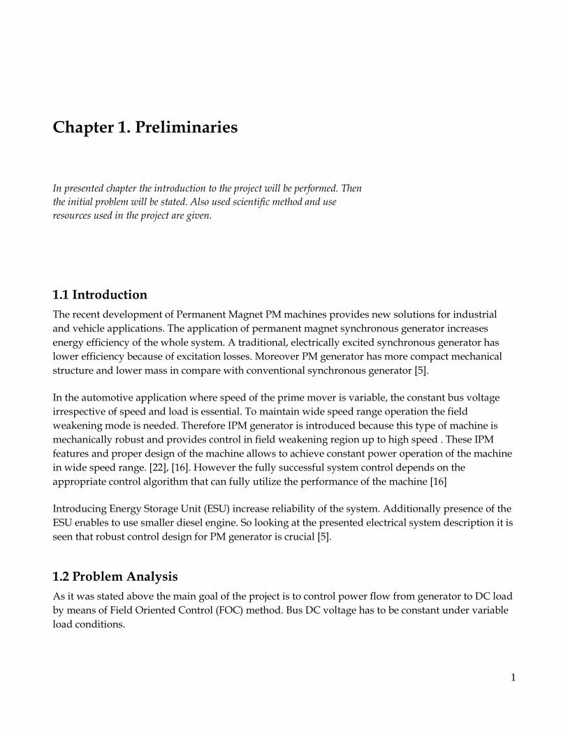
Chapter 1. Preliminaries

In presented chapter the introduction to the project will be performed. Then

the initial problem will be stated. Also used scientific method and use

resources used in the project are given.

1.1 Introduction

The recent development of Permanent Magnet PM machines provides new solutions for industrial

and vehicle applications. The application of permanent magnet synchronous generator increases

energy efficiency of the whole system. A traditional, electrically excited synchronous generator has

lower efficiency because of excitation losses. Moreover PM generator has more compact mechanical

structure and lower mass in compare with conventional synchronous generator [5].

In the automotive application where speed of the prime mover is variable, the constant bus voltage

irrespective of speed and load is essential. To maintain wide speed range operation the field

weakening mode is needed. Therefore IPM generator is introduced because this type of machine is

mechanically robust and provides control in field weakening region up to high speed . These IPM

features and proper design of the machine allows to achieve constant power operation of the machine

in wide speed range. [22], [16]. However the fully successful system control depends on the

appropriate control algorithm that can fully utilize the performance of the machine [16]

Introducing Energy Storage Unit (ESU) increase reliability of the system. Additionally presence of the

ESU enables to use smaller diesel engine. So looking at the presented electrical system description it is

seen that robust control design for PM generator is crucial [5].

1.2 Problem Analysis

As it was stated above the main goal of the project is to control power flow from generator to DC load

by means of Field Oriented Control (FOC) method. Bus DC voltage has to be constant under variable

load conditions.

1

Generator used in considered system is Interior mounted Permanent Magnet Synchronous Generator

(IPMSG). Output DC bus voltage is controlled by AC/DC power electronics converter installed

between generator and DC link.

The main schemes of three-phase PM generator and AC/DC converters system are:

Generator with classic six-pulse diode rectifier

Generator with boost type chopper converter

Generator with boost PWM rectifier

1.2.1 Generator with six-pulse diode rectifier

The diode rectifier is very common device in power electronics systems. It has simple topology and

does not need sophisticated control devices. However diode rectifier generates harmonic currents to

the ac side and also allows only one side power flow [3]. Moreover DC link voltage control in system

where diode rectifier is attached to PM generator (so excitation current is constant in linear region of

work) is only possible by means of varying generator speed. Therefore when generator is running in

variable speed mode it is problematic to keep constant DC link bus voltage in this solution.

Fig 1.1.Uncontrolled diode rectifier coupled generator (BLDC in that case) [6].

1.2.2 Generator with boost type chopper converter

To overcome disadvantages of diode rectifier many techniques have been proposed. The converter

presented below consists of diode rectifier and PWM boost chopper transistor [3]. This converter gives

maximum output DC voltage (opposite to diode rectifier where output voltage is always lower then

supply voltage) [3].

2

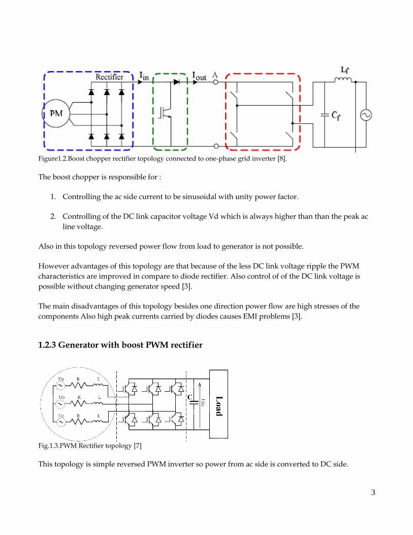
Figure1.2.Boost chopper rectifier topology connected to one-phase grid inverter [8].

The boost chopper is responsible for :

1. Controlling the ac side current to be sinusoidal with unity power factor.

2. Controlling of the DC link capacitor voltage Vd which is always higher than than the peak ac

line voltage.

Also in this topology reversed power flow from load to generator is not possible.

However advantages of this topology are that because of the less DC link voltage ripple the PWM

characteristics are improved in compare to diode rectifier. Also control of of the DC link voltage is

possible without changing generator speed [3].

The main disadvantages of this topology besides one direction power flow are high stresses of the

components Also high peak currents carried by diodes causes EMI problems [3].

1.2.3 Generator with boost PWM rectifier

Fig.1.3.PWM Rectifier topology [7]

This topology is simple reversed PWM inverter so power from ac side is converted to DC side.

3

Therefore bi-directional power flow is allowed with this topology. The DC voltage is higher than peak

ac voltage. The control strategy of PWM rectifier provides sinusoidal ac current and unity power

factor [3].

The main disadvantages of this converter topology are: requirements for sophisticated control devices

and high switching frequency losses [1].

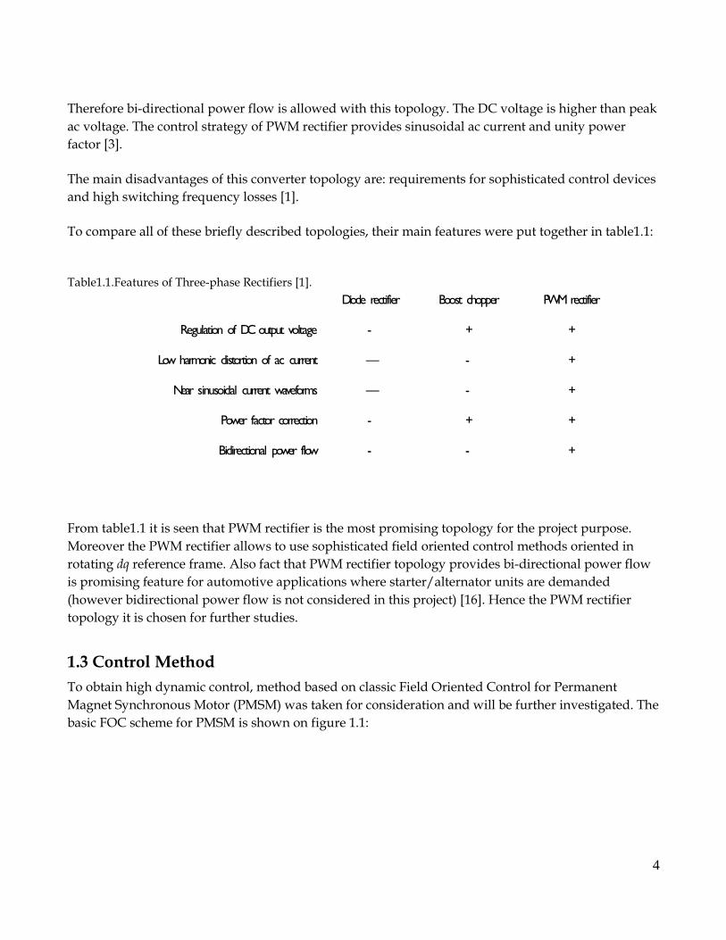
To compare all of these briefly described topologies, their main features were put together in table1.1:

Table1.1.Features of Three-phase Rectifiers [1].

Diode rectifier Boost chopper PWM rectifier

Regulation of DC output voltage - + +

Low harmonic distortion of ac current — - +

Near sinusoidal current waveforms — - +

Power factor correction - + +

Bidirectional power flow - - +

From table1.1 it is seen that PWM rectifier is the most promising topology for the project purpose.

Moreover the PWM rectifier allows to use sophisticated field oriented control methods oriented in

rotating dq reference frame. Also fact that PWM rectifier topology provides bi-directional power flow

is promising feature for automotive applications where starter/alternator units are demanded

(however bidirectional power flow is not considered in this project) [16]. Hence the PWM rectifier

topology it is chosen for further studies.

1.3 Control Method

To obtain high dynamic control, method based on classic Field Oriented Control for Permanent

Magnet Synchronous Motor (PMSM) was taken for consideration and will be further investigated. The

basic FOC scheme for PMSM is shown on figure 1.1:

4

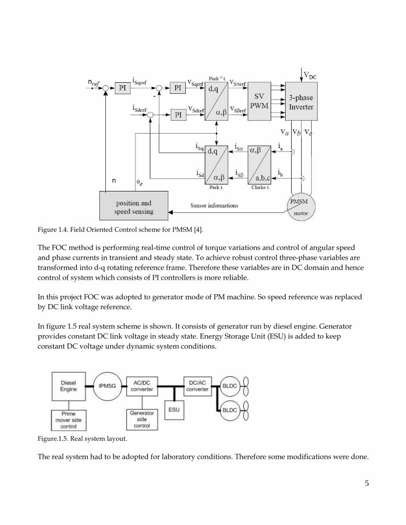
Figure 1.4. Field Oriented Control scheme for PMSM [4].

The FOC method is performing real-time control of torque variations and control of angular speed

and phase currents in transient and steady state. To achieve robust control three-phase variables are

transformed into d-q rotating reference frame. Therefore these variables are in DC domain and hence

control of system which consists of PI controllers is more reliable.

In this project FOC was adopted to generator mode of PM machine. So speed reference was replaced

by DC link voltage reference.

In figure 1.5 real system scheme is shown. It consists of generator run by diesel engine. Generator

provides constant DC link voltage in steady state. Energy Storage Unit (ESU) is added to keep

constant DC voltage under dynamic system conditions.

Figure.1.5. Real system layout.

The real system had to be adopted for laboratory conditions. Therefore some modifications were done.

5

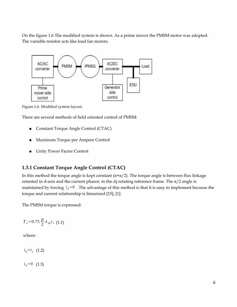
On the figure 1.6 The modified system is shown. As a prime mover the PMSM motor was adopted.

The variable resistor acts like load fan motors.

Figure.1.6. Modified system layout.

There are several methods of field oriented control of PMSM:

Constant Torque Angle Control (CTAC)

Maximum Torque per Ampere Control

Unity Power Factor Control

1.3.1 Constant Torque Angle Control (CTAC)

In this method the torque angle is kept constant (α=π/2). The torque angle is between flux linkage

oriented in d-axis and the current phasor, in the dq rotating reference frame. The π/2 angle is

maintained by forcing id=0 . The advantage of this method is that it is easy to implement because the

torque and current relationship is linearized [15], [1].

The PMSM torque is expressed:

T e=0.75p2 fd i s (1.1)

where:

iq=is (1.2)

id=0 (1.3)

6

The i s current for a given torque T e can be calculated:

i s=T e

0.75p2 fd

(1.4)

The air gap flux linkages can be described as:

m= fd2 Ld

2 id2 0.5

(1.5)

Because the id=0 this method is common for Surface Permanent Magnet Synchronous Machines

(SPMSM) . For IPMSM the reluctance torque cannot be utilized in this method. Hence for IPM with

high saliency ratio this is not recommended to use this method [15].

Zero d-axis current also occurs in the higher air gap flux linkage and higher back emf in result [15], [1]

1.3.2 Maximum Torque per Ampere Control

In this method the stator current is minimized for given torque. Therefore copper losses are

minimized. The iq and id currents are optimized by pre-defined functions derived from maximum

torque per stator current curve (figure 1.7).

7

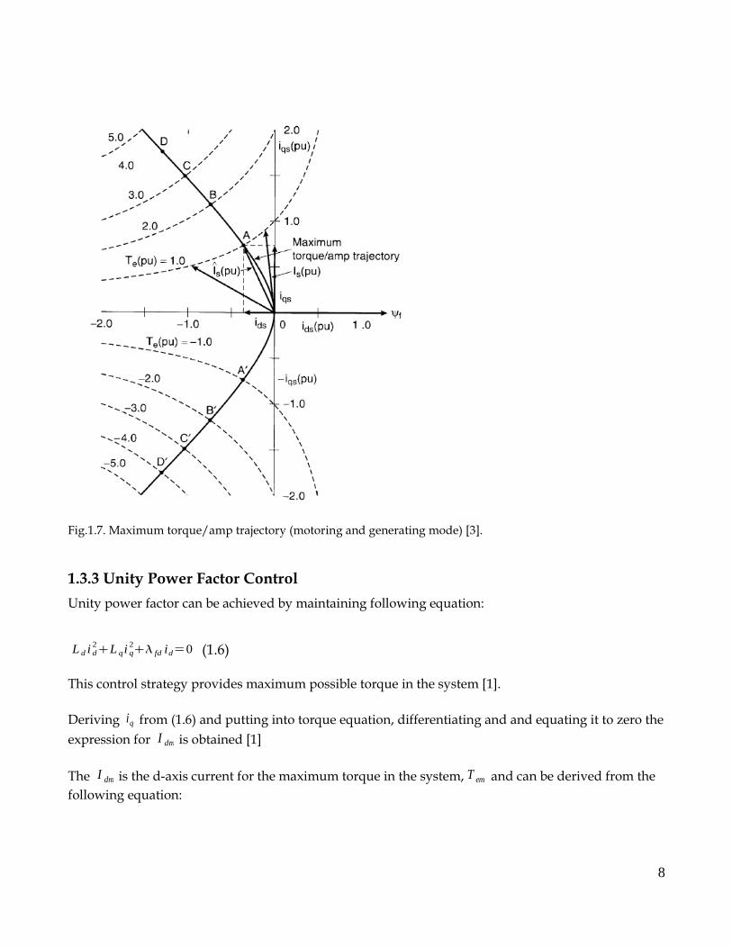
Fig.1.7. Maximum torque/amp trajectory (motoring and generating mode) [3].

1.3.3 Unity Power Factor Control

Unity power factor can be achieved by maintaining following equation:

L d i d2L qi q

2 fd id=0 (1.6)

This control strategy provides maximum possible torque in the system [1].

Deriving iq from (1.6) and putting into torque equation, differentiating and and equating it to zero the

expression for I dm is obtained [1]

The I dm is the d-axis current for the maximum torque in the system, T em and can be derived from the

following equation:

8

I dm2 I dm=0 (1.7)

where:

=4 LdLq Ld (1.8)

=3L dL q fd2 fd Ld (1.9)

= fd2

(1.10)

Putting I dm into (1.7) yields I qm at the maximum torque point. Inserting these two currents into

torque equation yields maximum torque for UPFC strategy [1].

1.4 Comparison and Selection of the Described Control Methods

1.4.1 Analysis

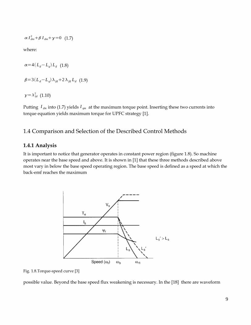
It is important to notice that generator operates in constant power region (figure 1.8). So machine

operates near the base speed and above. It is shown in [1] that these three methods described above

most vary in below the base speed operating region. The base speed is defined as a speed at which the

back-emf reaches the maximum

Fig. 1.8.Torque-speed curve [3]

possible value. Beyond the base speed flux weakening is necessary. In the [18] there are waveform

9

plots shown. In these waveforms it is seen that the important factors such as torque, power factor,

back emf and current are different for each method mainly below the base speed. Beyond the base

speed the waveforms of each methods are close to each other. Therefore for the studied generator

system purposes the leading selection criterion is the easy way to implement the control algorithm in

DSP.

1.4.2 The Method Selection

Taking into account conclusions written above the most promising method to use is CTAC. However

the machine used in the project is interior permanent magnet type. Therefore it seems that this method

is not suitable for this application. However as it was written before it depends on the machine

saliency ratio.

The saliency ratio of the machine used in the project is:

LqLd

=47.2 uH28.7uH

=1.64 (1.11)

So the saliency ratio is not that high (some machines has saliency ratio around five)

Therefore regarding to the low saliency factor of the used machine and fact that CTAC method is easy

to implement , this method was selected for further studies.

1.5 Scope on the Project

The PWM rectifier converter topology and FOC control method were selected in this project. FOC

method which utilizes PWM rectifier will be studied during a project work.

The FOC method also will be implemented in Digital Signal Processor (DSP) by means of TI C2000

Simulink toolbox and Code Composer Studio software to control the generator in scaled-down

laboratory set-up.

1.6 .Objective

The objective of this project was to study ,optimize and implement selected method which is reliable

for DC Link Voltage robust control.

The project does not deal with mechanical noise of the machine, thermal problems, EMC problems,

influence of the environmental factors on the system.

10

Magnetic saturation problems are also neglected despite fact that these problems are significant

phenomena during operating the IPM machine [16].

The reason of neglecting magnetic saturation is described in [18]- in higher speeds region this effect

has not that sufficient influence on working IPM characteristics (in this project generator is running

close to base speed and above) [18].

1.7 .Resources and Tools

1.7.1 Resources

The IPM generator is a three phase prototype designed by Sauer-Danfoss. It is 12

pole machine, designed to be supplied by a 24V power supply and it has rated power 2,2kW.

The available BPI is also from Sauer-Danfoss and its target applications are

battery powered mobile vehicles. It has a rated maximum continuous

power at 7kW and its nominal supply voltage is 48V, but is only supplied by

24V due to the voltage rating of the generator. The BPI is a modified

type BPI 5435.

The modification is due to a mounted interface board, which

accepts optical PWM signals from an external source. The BPI has a built in

dead time generator to provide protection against shoot through.

At the shaft of the IPM generator an encoder is mounted, so the rotor position is obtained. The

encoder gives 10:000 Quadric Encoded Pulses (QEP) per revolution.

Th machine used in project as prime mover is a three-phase brushless servo permanent magnet motor

made by Siemens. It is supplied by three-phase 380 voltage and it

has rated torque Tn=12 Nm and rated speed n=4500 rpm. The motor is controlled by Siemens 6SE7022

inverter.

To implement a real-time control and measure drive system performance, the TMS320F2812 Digital

11

Signal Processor (DSP) from Texas Instruments is used. The selected DSP is designed for industrial

control applications. It has 32 bit fixed point core, 12 bit ADC converters (16 channel), and 6 PWM

outputs.

1.7.2 Tools

The model of FOC control of IPM generator was built and tested in Simulink software environment.

The Simulink model has been performed to understand and predict behavior of the controller .

The controller model then has to be discretized and the new model is built in Simulink toolbox TI

C2000 DSP (where control system tested in Simulink is used and the whole system using TI C2000

DSP blocks is built) .

The Simulink model is enclosed in the attached CD-ROM .

1.8 Initial problem

As it was written before the design of the proper control method for IPM generator is the goal of this

project.. Therefore the initial problem could be written as:

Design of a DC Link Voltage control strategy for IPMSG.

1.9 The Structure of the Project

This report is a documentation of performed project work. The report contains a main report,

appendices and enclosed CD-ROM.

In order to be able to control the IPM generator a motor model based on mathematical equations was

performed.

To reduce complexity of the model, effects such temperature variations, saturation or non-sinusoidal

winding distribution are neglected.

In chapter 1 necessary introduction to project is presented. Description of the project goals and

available resources are written. The review of the available converter topologies are described and one

was selected for further investigation. Also some of FOC methods were presented and also one was

chosen .

In chapter 2 the principles and theory background of the models used in project are presented. All

models used in simulations are briefly described.

12

In chapter 3 the selected FOC method is explained. This chapter contains also description of PI

controllers design.

In chapter 4 the simulations results, hardware setup and the implementation of the controller in DSP

is described. The FOC control method is tested in laboratory. Then performance of the method is

evaluated.

The conclusions and future work tasks are written in chapter 5.

13

14

Chapter 2. Modelling

In this chapter mathematical models of the system parts such as generator,

AC/DC converter , DC link and load have been developed and built. The

SVM principles are also described here.

2.1 Modelling

This project deals with IPMSG which provides electric power in DC voltage fan drive system. The

load fan motors are BLDC type controlled by simple sensorless scheme and are supplied by ac/dc

converters. However for simulations purposes concentrated on dynamic behavior of the whole system

under variable load conditions simulation is focused on generator model and DC link side. The load

fan motors are replaced by simple variable resistor. In the real system as prime mover the diesel

engine is used. For modeling purposes the diesel engine is replaced by Permanent Magnet

Synchronous Motor (PMSM) controlled by means of Field Oriented Control.

2.1.1 Permanent Magnet Machine Model

In the simulated system there are two permanent magnet machines used one as prime mover and one

as generator. That for motor is surface magnet mounted type and that for generator is interior magnet

mounted type. Therefore the same model could be used for both machines. However for generator

sign conversion has to be taken into account.

In the figure 2.1 Permanent Magnet Synchronous Machine is presented. It is seen that the d-axis is

aligned with a-axis.

.

15

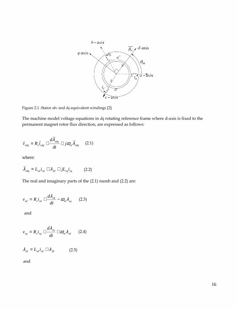
Figure 2.1 .Stator abc and dq equivalent windings [2].

The machine model voltage equations in dq rotating reference frame where d-axis is fixed to the

permanent magnet rotor flux direction, are expressed as follows:

sdqmsdq

sdqssdq jdt

diRv λω

λ++= (2.1)

where:

sqsqfdsdsdsdq ijLiL ++= λλ (2.2)

The real and imaginary parts of the (2.1) numb and (2.2) are:

sqmsd

sdssd dt

diRv λωλ

−+= (2.3)

and

sdmsq

sqssq dt

diRv λω

λ++= (2.4)

fdsdsdsd iL λλ += (2.5)

and

16

sqsqsq iL=λ (2.6)

Putting (2.5) to (2.3) and (2.6) to (2.4) we can obtain:

sqsqmsd

sddssds iLdt

diLiRv ω−+= (2.7)

v sq=R si sqL sq

di sq

dtm Lsd isdm fd

(2.8)

where the electrical rotor speed m is related with mechanical rotor speed mech by expression:

m=p2mech (2.9)

The expression of electromagnetic torque is written by equation:

T em=p2

32sd i sqsqi sd (2.10)

Putting (2.5) and (2.6) into (2.10) the torque equation becomes:

T em=p2

32 fd i sq LsdLsqi sqi sd (2.11)

It is seen that IPMSM contains torque component because d and q inductances are not equal.

The acceleration of the machine is expressed by mechanical equation:

1J

dmech

dt=T emT L (2.12)

Where T L is the load torque.

In the generating mode power flows in reversed direction. Therefore to keep order in signs conversion

generator model has to be adopted and its equations were changed:

17

v sd=Rs isdL sd

di sd

dtm L sqi sq

(2.13)

v sq=Rs i sqL sq

di sq

dtm L sd i sdm fd

(2.14)

The mechanical equation for generating mode is:

1J

dmech

dt=T mechT em (2.15)

where T mech is torque produced by prime mover and T em in this case is produced by electrical load of

the generator.

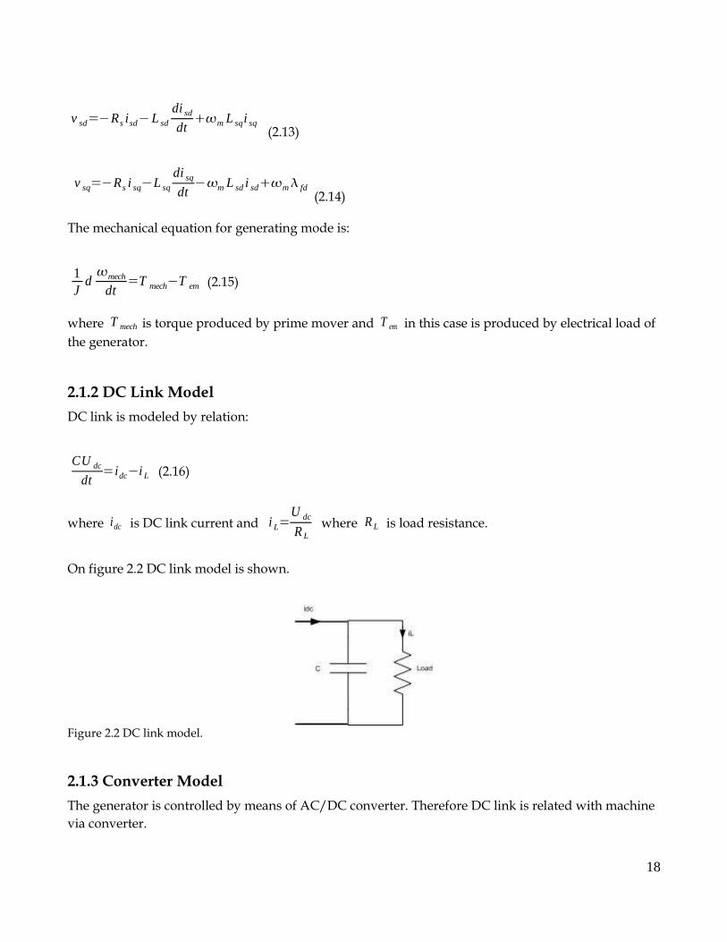
2.1.2 DC Link Model

DC link is modeled by relation:

CU dc

dt=idci L (2.16)

where idc is DC link current and i L=U dc

R L where R L is load resistance.

On figure 2.2 DC link model is shown.

Figure 2.2 DC link model.

2.1.3 Converter Model

The generator is controlled by means of AC/DC converter. Therefore DC link is related with machine

via converter.

18

The converter is a voltage source converter (VSC) working as a rectifier in generation mode where

power flows to the DC link.

Opposite to motoring mode in generation mode, model of the VSC is necessary because DC side

variables and AC side variables are controlled. Because of fact that system includes mechanical

components which time constants are significantly bigger than converter switching times, the average

VSC model is used without disturbing the final result.

The generator windings are star connected. Generator is connected to VSC.

Fort he star type connection the generator voltages are calculated using following equations [14]:

V A0=V ANV 0N=sA V DCV 0N=V DC

32s AsBsC (2.17)

V B0=V BNV 0N=s BV DCV 0N=V DC

3s A2s BsC (2.18)

V C0=V CNV 0N=sCV DCV 0N=V DC

3s AsB2sC (2.19)

Where V 0N is sum of line to neutral voltages ( V AN , V BN , V CN )

divided by 3:

V 0N=V ANV BNV CN

3=

V DC

3 sAs BsC (2.20)

The relations between generator voltages are shown in figure 2.3

19

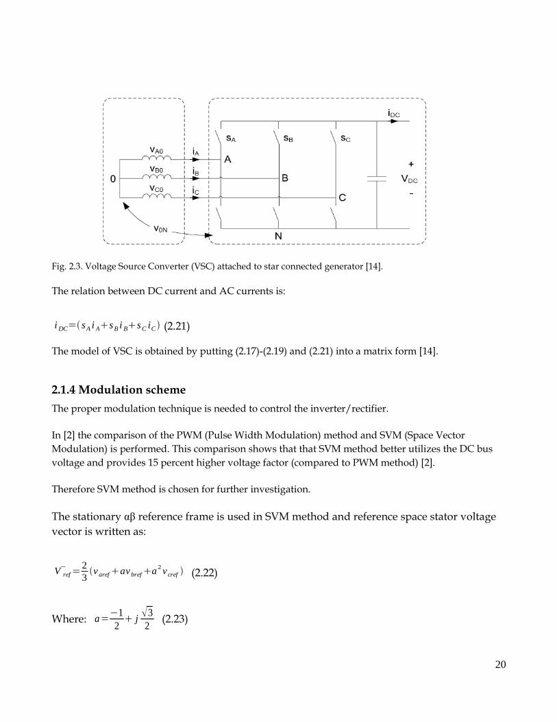
Fig. 2.3. Voltage Source Converter (VSC) attached to star connected generator [14].

The relation between DC current and AC currents is:

i DC= sA i AsB i BsC iC (2.21)

The model of VSC is obtained by putting (2.17)-(2.19) and (2.21) into a matrix form [14].

2.1.4 Modulation scheme

The proper modulation technique is needed to control the inverter/rectifier.

In [2] the comparison of the PWM (Pulse Width Modulation) method and SVM (Space Vector

Modulation) is performed. This comparison shows that that SVM method better utilizes the DC bus

voltage and provides 15 percent higher voltage factor (compared to PWM method) [2].

Therefore SVM method is chosen for further investigation.

The stationary αβ reference frame is used in SVM method and reference space stator voltage

vector is written as:

V ref=23varefavbrefa2 vcref (2.22)

Where: a=12 j 3

2 (2.23)

20

And varef , vbref and v cref are reference voltages in 3 phase abc reference frame.

The figure 2.4 shows reference voltage vector projection.

Fig. 2.4. Basic voltage vectors [12].

It is seen that there are eight possible combinations of the switches position (six active states, two zero

states).

Therefore to create desired voltage vector in preset sector within the reference frame (fig 2.4), it is

essential to combine adjacent vectors of the reference voltage and to modulate them in proper time

period [15].

In the figure 2.4 reference voltage vector is located in sector 1 and adjacent state voltage

vectors are V 100 , V 110 . As it is seen in figure 2.4 the adjacent voltages are modulated by

specified time factors to obtain desired voltage vector.

In figure 2.5 the cycle for sector 1 is shown:

21

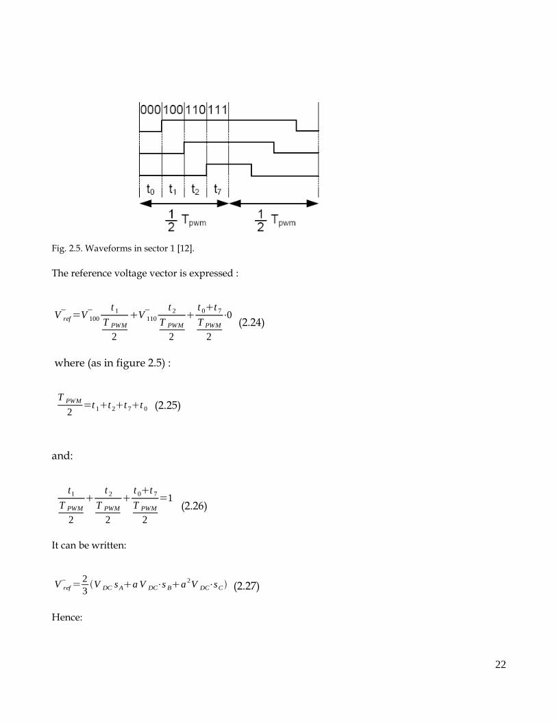
Fig. 2.5. Waveforms in sector 1 [12].

The reference voltage vector is expressed :

V ref= V 100

t 1

T PWM

2

V 110

t 2

T PWM

2

t 0t 7

T PWM

2

⋅0 (2.24)

where (as in figure 2.5) :

T PWM

2=t 1t 2t 7t 0 (2.25)

and:

t1

T PWM

2

t 2

T PWM

2

t 0t 7

T PWM

2

=1 (2.26)

It can be written:

V ref=23V DC sAa V DC⋅s Ba 2V DC⋅sC (2.27)

Hence:

22

V 100=23V DC⋅1aV DC⋅0a 2V DC⋅0=

23

V DC (2.28)

V 100=23V DC⋅1aV DC⋅1a 2 V DC⋅0 =

23

V DC12 j 3

2 (2.29)

The equation (2.24) can be expressed in complex form:

V ref=V ref cossin (2.30)

Further it is possible to distinguish real and imaginary part:

ℜ[ V ref ]=V ref cos=23

V DC

2t 1

T PWM

23

V DC

2t2

T PWM

cos 3

(2.31)

ℑ[ V ref ]=V ref sin =23

V DC

2t 2

T PWM

sin 3

(2.32)

From (2.31) and (2.32) the time durations for active states in sector 1 can be calculated:

t 1=3V ref

V DC

T PWM

2sin 60 o (2.33)

t 2=3V ref

V DC

T PWM

2sin (2.34)

From waveforms in the figure 2.5 , the duty cycles for control converter can be calculated.

sA=t 1t 2t7

T PWM

2 (2.35)

sA=t 2t 7

T PWM

2 (2.36)

23

sA=t 7

T PWM

2 (2.37)

The procedure to obtain these times for each sector is similar [1].

2.2 Summary

In this chapter mathematical models of the system components were derived and presented. Also

SVM scheme for AC/DC converter was described. The system models are realized in continuous

domain and are used as connected together to simulate behavior of the whole generator system.

24

25

Chapter 3. Control System

In this chapter the selected field oriented control method is explained. Also

the flux weakening algorithm is described. In the second part of the chapter

the machine controller design is performed.

3.1 Field Oriented Control of the Generator

A constant speed IPM generator is controlled via PWM rectifier. The vector oriented control is applied

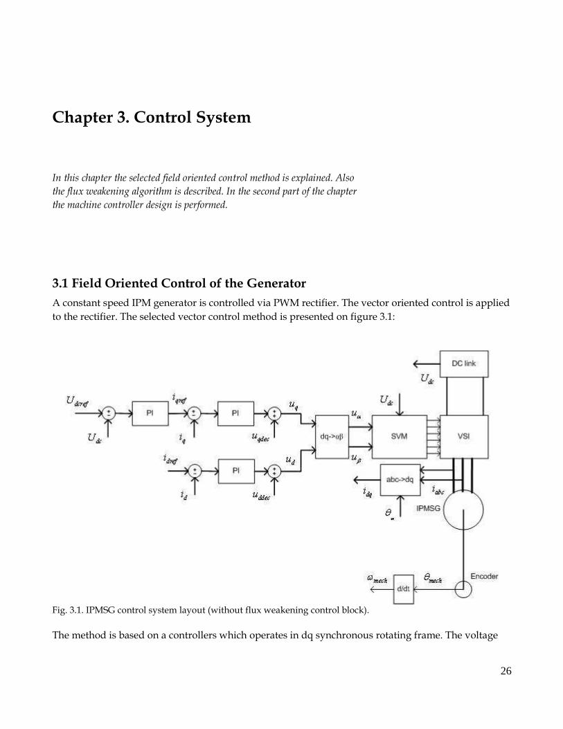
to the rectifier. The selected vector control method is presented on figure 3.1:

Fig. 3.1. IPMSG control system layout (without flux weakening control block).

The method is based on a controllers which operates in dq synchronous rotating frame. The voltage

26

controller gives i sq as a reference to the rectifier controller. Because CTAC method was applied the

i sd is equal to zero. In result the phase current is in a phase with back emf (BEMF) [9].

To eliminate the coupling terms between d and q, the decoupling network has been introduced.

3.2 Field Oriented Control

3.2.1 Field Oriented Control for Base Speed

The Field Oriented Control (FOC) method provides robust control of the PMSM. In Chapter 2 the dq

model of PMSM was presented. The reason of development dq model is that the FOC method is

oriented in dq synchronous rotating reference frame. The electrical equations for PMSM dq model

(generator convection) are as follows:

v sd=Rs isdL sd

di sd

dtm L sqi sq

(3.1)

v sq=Rs i sqL sq

di sq

dtm L sd i sdm fd

(3.2)

Electromagnetic torque is expressed:

T em=p2

32 fd i sq LsdLsqi sqi sd (3.3)

Putting equations (3.1), (3.2) into s-domain (replacing d/dt by Laplace's operator s) , the relations for

i sd and for i sq can be derived:

v sd=Rs isdLsd si sdm Lsq isq (3.4)

v sq=Rs i sqL sq si sqm Lsd i sdm fd (3.5)

Defining stator electrical time constants:

T sd=L sd

Rs

(3.6)

27

T sq=Lsq

R s

(3.7)

Equations (3.4) and (3.5) could be written:

m Lsq isqvsd=Rs1sT sd i sd (3.8)

m fdvsqm Lsd i sd=Rs1sT sq i sq (3.9)

And currents are expressed as:

i sd=vsdm Lsq i sq

R s1sT sd (3.10)

i sq=vsqm Lsd i sdw fd

Rs1sT sq (3.11)

3.2.2 Flux weakening mode

The maximum voltage which can be delivered to the machine is limited by the DC link voltage:

V s=2Vdc / (3.12)

where:

V s=vd2vq

2 (3.13)

where:

vq=e Ld id fd (3.14)

vd=e Lq iq (3.15)

(Resistance drop is neglected)

Substituting equation (3.15), (3.14) and (3.12) into (3.13) [3]:

28

e Ld ide fd2e

2 Lq2 iq

2=4Vd

2

2 (3.16)

(3.16) can be rearranged [3]:

i d fd

Ld

2

2Vd

e Ld

2

i q2

2Vd

e Lq

2=1 (3.17)

It is seen that (3.17) is ellipse equation [3]:

idC 2

A2 i q

2

B=1 (3.18)

where:

A=2Vd

e Ld

(3.19) is the length of the semi major axis

B=2Vd

e Lq

(3.20) is the length of the semi major axis

C= fd

Ld

(3.21) is the offset of the ellipse center on the d-axis [3].

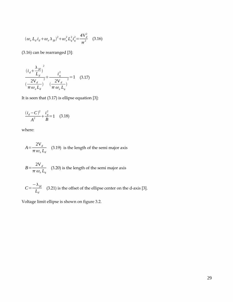
Voltage limit ellipse is shown on figure 3.2.

29

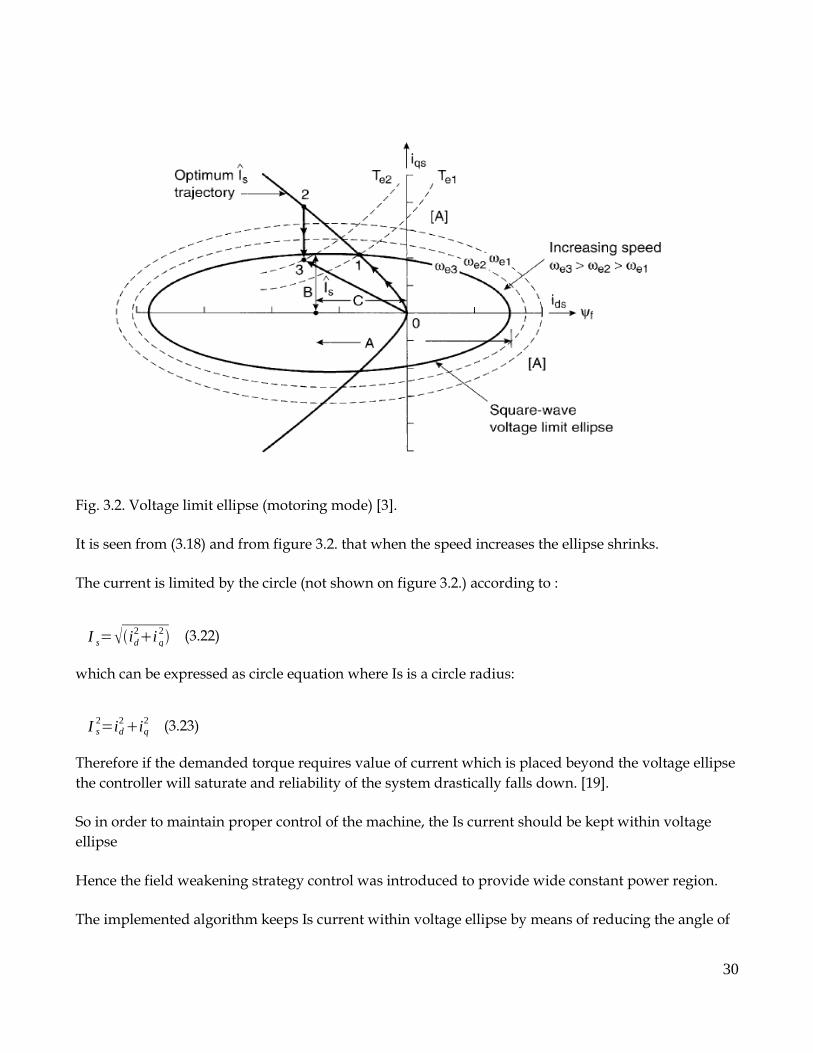
Fig. 3.2. Voltage limit ellipse (motoring mode) [3].

It is seen from (3.18) and from figure 3.2. that when the speed increases the ellipse shrinks.

The current is limited by the circle (not shown on figure 3.2.) according to :

I s=id2i q

2 (3.22)

which can be expressed as circle equation where Is is a circle radius:

I s2=id

2iq2 (3.23)

Therefore if the demanded torque requires value of current which is placed beyond the voltage ellipse

the controller will saturate and reliability of the system drastically falls down. [19].

So in order to maintain proper control of the machine, the Is current should be kept within voltage

ellipse

Hence the field weakening strategy control was introduced to provide wide constant power region.

The implemented algorithm keeps Is current within voltage ellipse by means of reducing the angle of

30

the commanded current (figure 3.3) [16].

Fig. 3.3. Flux weakening action by means of reducing angle (generating mode) [16].

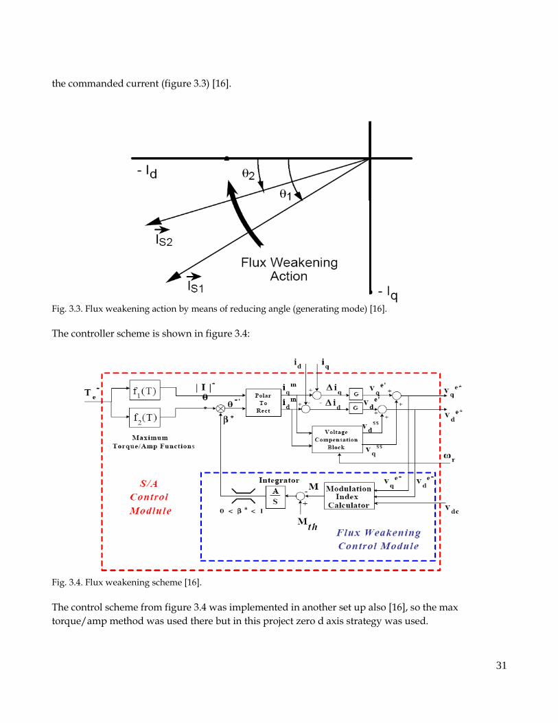
The controller scheme is shown in figure 3.4:

Fig. 3.4. Flux weakening scheme [16].

The control scheme from figure 3.4 was implemented in another set up also [16], so the max

torque/amp method was used there but in this project zero d axis strategy was used.

31

To get current angle dq currents are transformed into the polar coordinates where the angle is

multiplied by β which is :

01 (3.24)

β is a result of the error between calculated and referenced modulation index (which is around 1). In

the project instead integrator ,PI controller with anti-wind up was used. Current angle is changed by

multiplying it by β and the result seen on figure 3.3. is obtained.

Modulation Index Calculator calculates modulation index [16]:

M=vq

2vd2

V d2

(3.25)

From (3.25) it is seen that method is dependent on changing of the machine parameters.

3.3 Design of the Control System

The scheme of the selected control system is shown on figure 3.1.

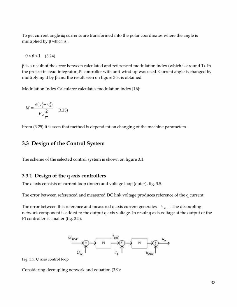
3.3.1 Design of the q axis controllers

The q axis consists of current loop (inner) and voltage loop (outer), fig. 3.5.

The error between referenced and measured DC link voltage produces reference of the q current.

The error between this reference and measured q axis current generates v sq . The decoupling

network component is added to the output q axis voltage. In result q axis voltage at the output of the

PI controller is smaller (fig. 3.5).

Fig. 3.5. Q axis control loop

Considering decoupling network and equation (3.9):

32

v decqvsq=R s1sT sq i sq (3.26)

where decoupling components are:

v decq= fdm L sd i sd (3.27)

The decoupling component (3.27) is considered as disturbance which is independent on the q axis

current. As in the [10] and [11] fed drives the current loop controller is designed at the beginning.

Design of the current controller (q axis)

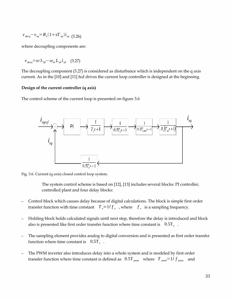
The control scheme of the current loop is presented on figure 3.6

Fig. 3.6. Current (q axis) closed control loop system.

The system control scheme is based on [12], [13] includes several blocks: PI controller,

controlled plant and four delay blocks:

– Control block which causes delay because of digital calculations. The block is simple first order

transfer function with time constant T s=1/ f s , where f s is a sampling frequency.

– Holding block holds calculated signals until next step, therefore the delay is introduced and block

also is presented like first order transfer function where time constant is 0.5T s .

– The sampling element provides analog to digital conversion and is presented as first order transfer

function where time constant is 0.5T s .

– The PWM inverter also introduces delay into a whole system and is modeled by first order

transfer function where time constant is defined as 0.5T pwm where T pwm=1/ f pwm and

33

f pwm is a switching frequency.

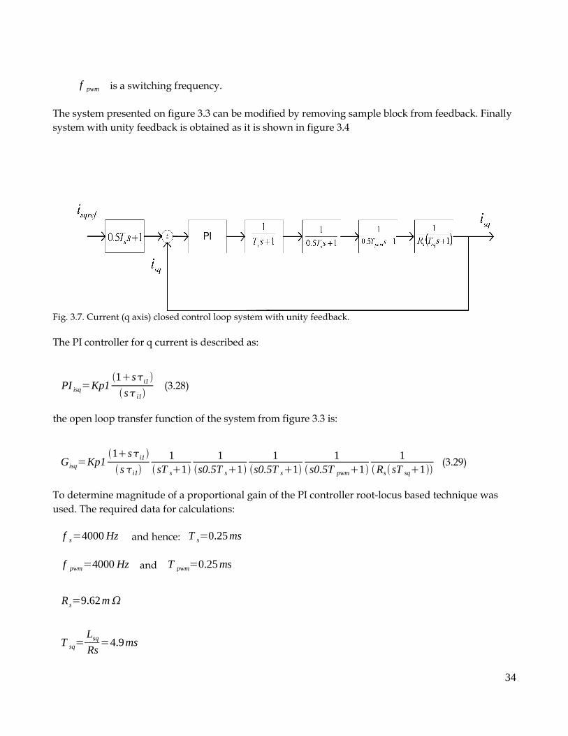
The system presented on figure 3.3 can be modified by removing sample block from feedback. Finally

system with unity feedback is obtained as it is shown in figure 3.4

Fig. 3.7. Current (q axis) closed control loop system with unity feedback.

The PI controller for q current is described as:

PI isq=Kp11si1

s i1 (3.28)

the open loop transfer function of the system from figure 3.3 is:

Gisq=Kp11si1

si11

sT s11

s0.5T s11

s0.5T s11

s0.5T pwm11

Rs sT sq1(3.29)

To determine magnitude of a proportional gain of the PI controller root-locus based technique was

used. The required data for calculations:

f s=4000 Hz and hence: T s=0.25 ms

f pwm=4000 Hz and T pwm=0.25 ms

R s=9.62m

T sq=Lsq

Rs=4.9ms

34

T determine maximum magnitude of a proportional gain of the PI controller root-locus based

technique was used.

The root-locus technique is performed in Matlab software environment.

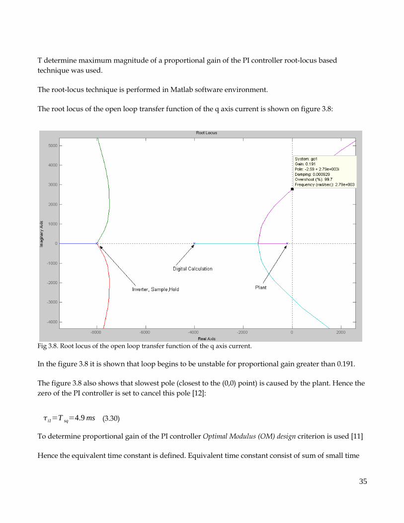
The root locus of the open loop transfer function of the q axis current is shown on figure 3.8:

Fig 3.8. Root locus of the open loop transfer function of the q axis current.

In the figure 3.8 it is shown that loop begins to be unstable for proportional gain greater than 0.191.

The figure 3.8 also shows that slowest pole (closest to the (0,0) point) is caused by the plant. Hence the

zero of the PI controller is set to cancel this pole [12]:

i1=T sq=4.9 ms (3.30)

To determine proportional gain of the PI controller Optimal Modulus (OM) design criterion is used [11]

Hence the equivalent time constant is defined. Equivalent time constant consist of sum of small time

35

constants:

T eq=2T s0.5Tpwm=0.625ms (3.17)

Using (3.30) and (3.31) the equation (3.29) is written as:

Gisq=Kp1 s i1

1R s sT eq1

(3.32)

In the OM method the damping factor =22

[11].

The generic open loop second order transfer function with damping factor =22

and time

constant defined as τ has form as:

GOM=1

21s (3.33)

To obtain Kpi equations (3.31) and (3.32) are compared, where =T eq and also using (3.30):

K pi1

T sq R s=

12Teq

(3.34)

and:

K pi1=T sq R s

2Teq (3.35)

Finally:

K pi1=0.0378

In the PI controller the proportional and integrator gains are related:

36

Ki=Kp

(3.36)

Hence:

Ki1=K p1

i1=7.71 (3.37)

The figure 3.9 shows zero-pole map of the designed control loop. From the figure 3.9 it is seen that

designed loop is stable.

Fig.3.9. Zero-pole map of the q axis current control loop (closed loop transfer function).

The figure 3.10 shows bode plot of the designed controller system.

37

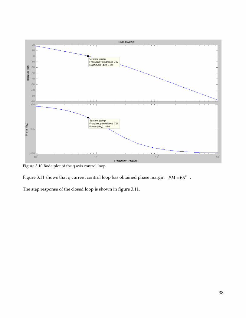
Figure 3.10 Bode plot of the q axis control loop.

Figure 3.11 shows that q current control loop has obtained phase margin PM=65o .

The step response of the closed loop is shown in figure 3.11.

38

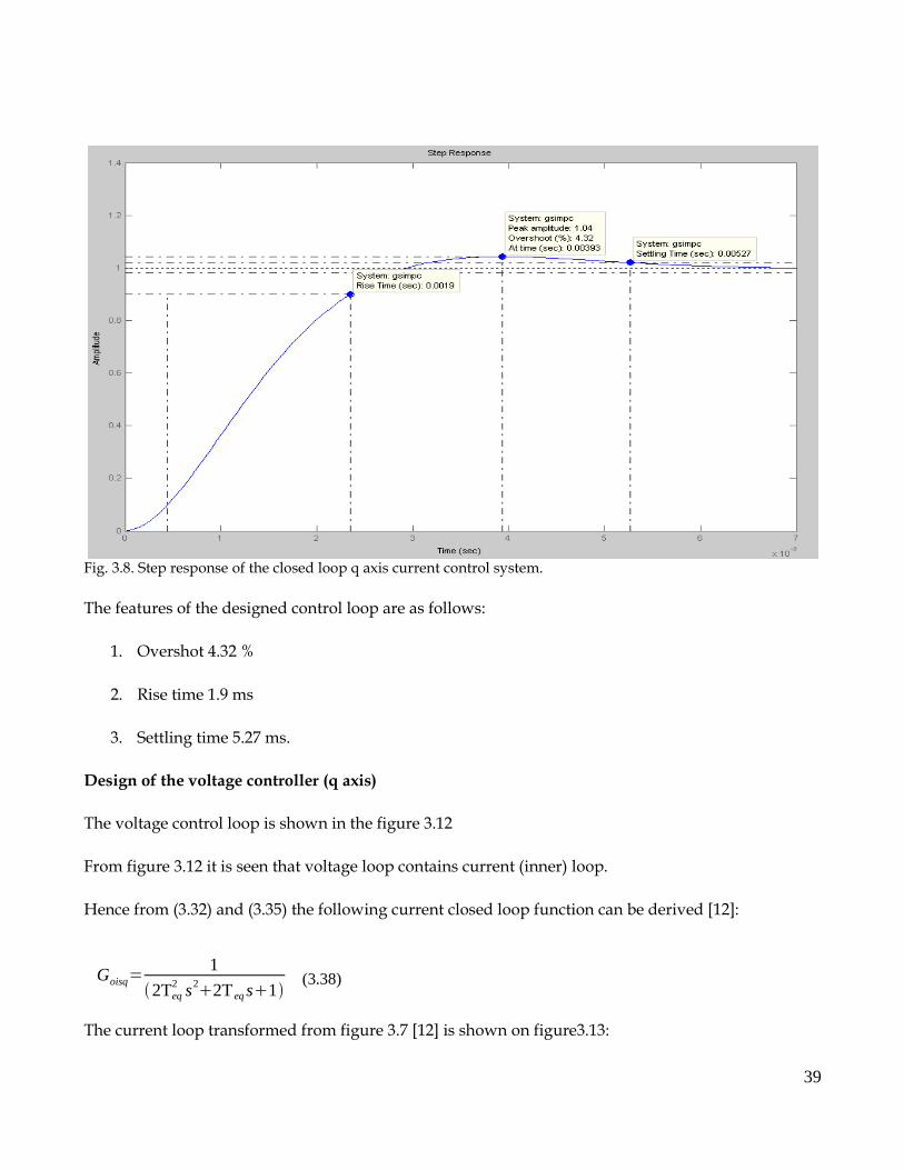
Fig. 3.8. Step response of the closed loop q axis current control system.

The features of the designed control loop are as follows:

1. Overshot 4.32 %

2. Rise time 1.9 ms

3. Settling time 5.27 ms.

Design of the voltage controller (q axis)

The voltage control loop is shown in the figure 3.12

From figure 3.12 it is seen that voltage loop contains current (inner) loop.

Hence from (3.32) and (3.35) the following current closed loop function can be derived [12]:

Goisq=1

2Teq2 s22T eq s1

(3.38)

The current loop transformed from figure 3.7 [12] is shown on figure3.13:

39

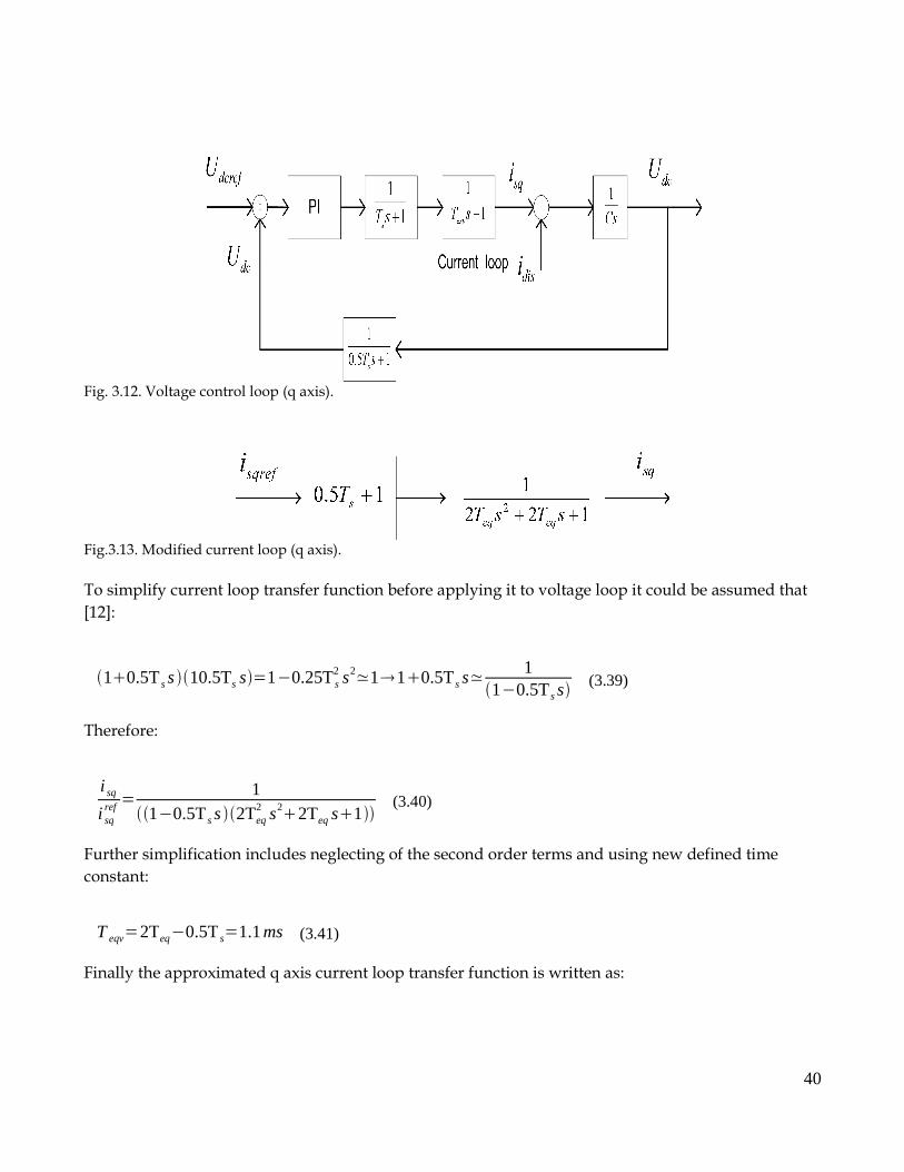
Fig. 3.12. Voltage control loop (q axis).

Fig.3.13. Modified current loop (q axis).

To simplify current loop transfer function before applying it to voltage loop it could be assumed that

[12]:

10.5T s s 10.5Ts s=10.25T s2 s2≃110.5T s s≃

110.5T s s (3.39)

Therefore:

i sq

i sqref =

110.5T s s 2Teq

2 s22Teq s1 (3.40)

Further simplification includes neglecting of the second order terms and using new defined time

constant:

T eqv=2Teq0.5T s=1.1 ms (3.41)

Finally the approximated q axis current loop transfer function is written as:

40

i sq

i sqref =

11T eqv s

(3.42)

The voltage control loop from figure 3.9 contains previously derived current control loop (3.42) and

similarly to current loop contains also PI controller and delay blocks [11], [12] :

1. Digital calculations block which is as previously first order transfer function T s=1/ f s wher f s isa sampling frequency.

2. Digital to analog conversion block which is presented like first order transfer function with time constant0.5T s

The DC link voltage is calculated using the relation between currents in DC link:

CdU dc

dt=i dciload (3.43)

where iload is equal to U dc

Rload

(3.44)

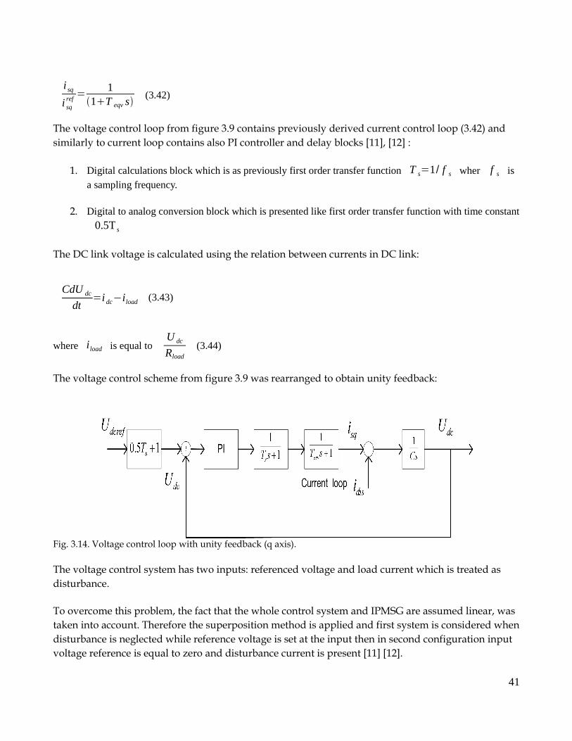
The voltage control scheme from figure 3.9 was rearranged to obtain unity feedback:

Fig. 3.14. Voltage control loop with unity feedback (q axis).

The voltage control system has two inputs: referenced voltage and load current which is treated as

disturbance.

To overcome this problem, the fact that the whole control system and IPMSG are assumed linear, was

taken into account. Therefore the superposition method is applied and first system is considered when

disturbance is neglected while reference voltage is set at the input then in second configuration input

voltage reference is equal to zero and disturbance current is present [11] [12].

41

In the first situation where disturbance signal is set to zero only a proportional controller is enough to

fulfill system requirements [11] [12]. Hence only P component of the PI controller is studied.

The PI controller of the voltage loop:

PI v=Kp11sv

sv (3.45)

When the disturbance input is set to zero the open loop transfer function is:

G v=Kp31sv

sv1

sT s11

s0.5T s11

sT eqv11

sC (3.46)

where C is the DC link capacitor value.

New equivalent time constant is defined:

T sv=1.5T sT eqv=1.5ms (3.47)

And rearranged open loop transfer function is:

G v=Kp31sv

sv1

sT sv11

sC (3.48)

For loot locus analysis only proportional gain is considered:

G v=Kp31

sT sv11

sC (3.49)

The figure 3.12 shows root locus of the voltage controller open loop transfer function (3.49).

42

Fig. 3.15. Root locus of the voltage open loop transfer function.

The figure 3.15 shows that voltage loop is stable for any controller proportional gain.

The OM criterion is used to calculate the proper proportional voltage controller gain value [11]. As it was it was

before the damping factor is set up to = 22

. Following the procedure the (3.) is compared to generic

second order transfer function with preset damping factor (3.33) where =T sv .

Kp31C=

12Tsv

(3.50)

Kp3=C

2Tsv =6.8 (3.51)

To calculate time constant of the voltage loop PI controller the input reference voltage is set to zero

and disturbance signal which is a load current in this case is present.

The analysied set up is presented in figure 3.15

43

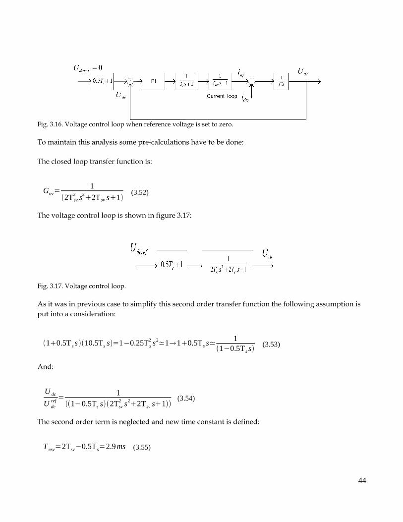
Fig. 3.16. Voltage control loop when reference voltage is set to zero.

To maintain this analysis some pre-calculations have to be done:

The closed loop transfer function is:

Gov=1

2T sv2 s22T sv s1

(3.52)

The voltage control loop is shown in figure 3.17:

Fig. 3.17. Voltage control loop.

As it was in previous case to simplify this second order transfer function the following assumption is

put into a consideration:

10.5T s s 10.5Ts s=10.25T s2 s2≃110.5T s s≃

110.5T s s

(3.53)

And:

U dc

U dcref =

110.5Ts s2Tsv

2 s22T sv s1(3.54)

The second order term is neglected and new time constant is defined:

T esv=2Tsv0.5T s=2.9ms (3.55)

44

Therefore (3.54) becomes:

U dc

U dcref =

11T esv s

(3.56)

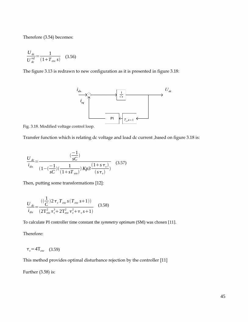
The figure 3.13 is redrawn to new configuration as it is presented in figure 3.18:

Fig. 3.18. Modified voltage control loop.

Transfer function which is relating dc voltage and load dc current ,based on figure 3.18 is:

U dc

idis

=1sC

11sC

1

1sT esv Kp3

1sv

sv

(3.57)

Then, putting some transformations [12]:

U dc

idis

=

1C2v T esv s T esv s1

2Tesv2 v

32Tesv2 v

2v s1 (3.58)

To calculate PI controller time constant the symmetry optimum (SM) was chosen [11].

Therefore:

v=4Tesv (3.59)

This method provides optimal disturbance rejection by the controller [11]

Further (3.58) is:

45

U dc

idis

=8Tesv s2 T esv s1

C8T esv3 v

38Tesv2 v

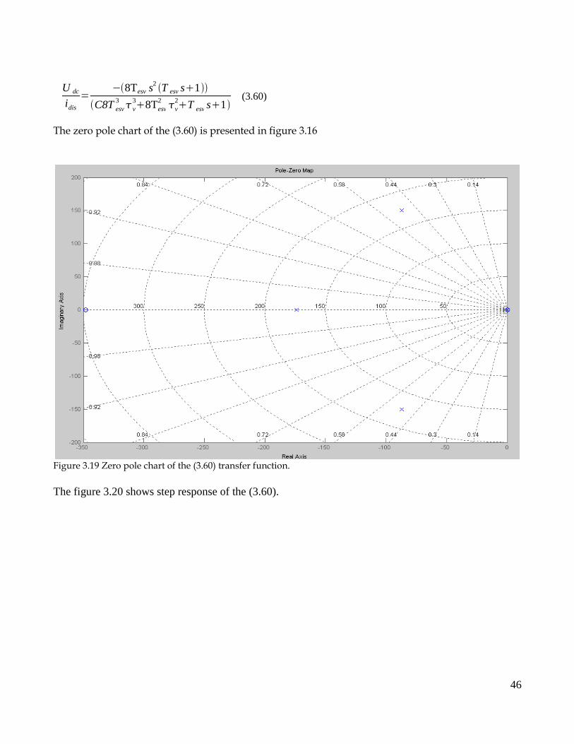
2T esv s1 (3.60)

The zero pole chart of the (3.60) is presented in figure 3.16

Figure 3.19 Zero pole chart of the (3.60) transfer function.

The figure 3.20 shows step response of the (3.60).

46

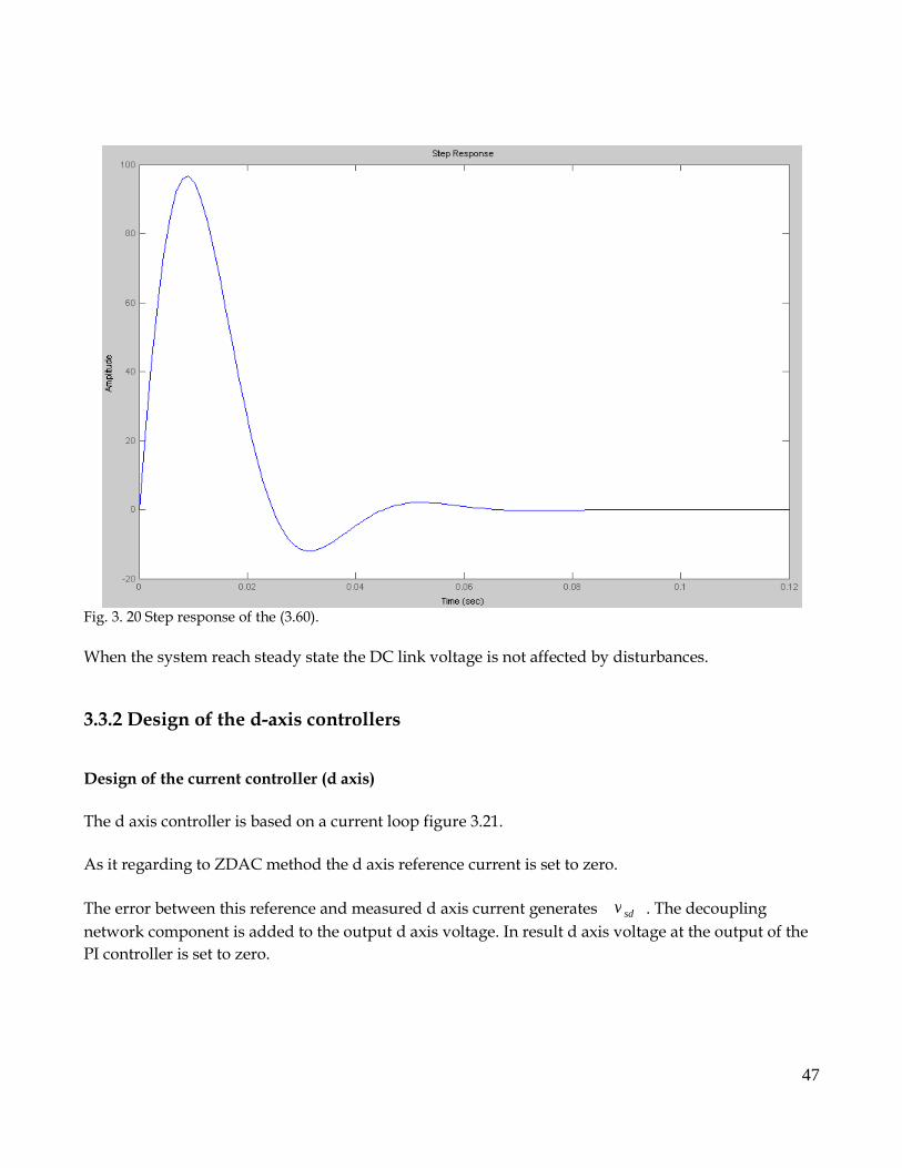
Fig. 3. 20 Step response of the (3.60).

When the system reach steady state the DC link voltage is not affected by disturbances.

3.3.2 Design of the d-axis controllers

Design of the current controller (d axis)

The d axis controller is based on a current loop figure 3.21.

As it regarding to ZDAC method the d axis reference current is set to zero.

The error between this reference and measured d axis current generates v sd . The decoupling

network component is added to the output d axis voltage. In result d axis voltage at the output of the

PI controller is set to zero.

47

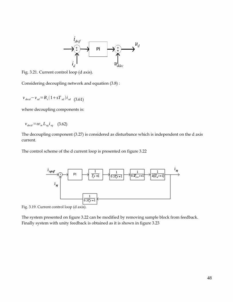
Fig. 3.21. Current control loop (d axis).

Considering decoupling network and equation (3.8) :

v decdvsd=R s1sT sd i sd (3.61)

where decoupling components is:

vdecd=m Lsq i sq (3.62)

The decoupling component (3.27) is considered as disturbance which is independent on the d axis

current.

The control scheme of the d current loop is presented on figure 3.22

Fig. 3.19. Current control loop (d axis).

The system presented on figure 3.22 can be modified by removing sample block from feedback.

Finally system with unity feedback is obtained as it is shown in figure 3.23

48

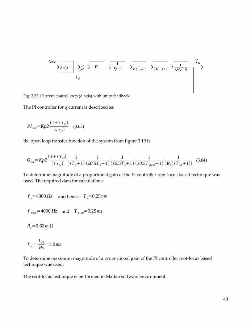
Fig. 3.23. Current control loop (d axis) with unity feedback.

The PI controller for q current is described as:

PI isd=Kp21si2

si2 (3.63)

the open loop transfer function of the system from figure 3.19 is:

Gisd=Kp21s i2

si21

sT s11

s0.5T s11

s0.5T s11

s0.5T pwm11

R s sT sd1(3.64)

To determine magnitude of a proportional gain of the PI controller root-locus based technique was

used. The required data for calculations:

f s=4000 Hz and hence: T s=0.25 ms

f pwm=4000 Hz and T pwm=0.25 ms

R s=9.62m

T sd=Lsd

Rs=3.0ms

To determine maximum magnitude of a proportional gain of the PI controller root-locus based

technique was used.

The root-locus technique is performed in Matlab software environment.

49

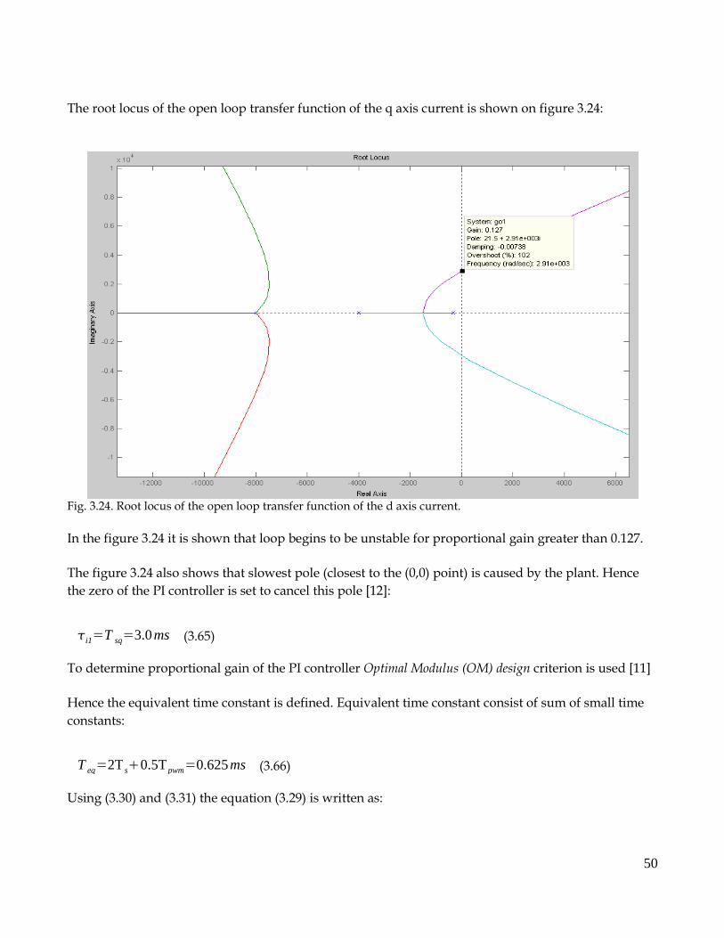
The root locus of the open loop transfer function of the q axis current is shown on figure 3.24:

Fig. 3.24. Root locus of the open loop transfer function of the d axis current.

In the figure 3.24 it is shown that loop begins to be unstable for proportional gain greater than 0.127.

The figure 3.24 also shows that slowest pole (closest to the (0,0) point) is caused by the plant. Hence

the zero of the PI controller is set to cancel this pole [12]:

i1=T sq=3.0ms (3.65)

To determine proportional gain of the PI controller Optimal Modulus (OM) design criterion is used [11]

Hence the equivalent time constant is defined. Equivalent time constant consist of sum of small time

constants:

T eq=2T s0.5Tpwm=0.625ms (3.66)

Using (3.30) and (3.31) the equation (3.29) is written as:

50

Gisd=Kp2 si2

1R s sT eq1

(3.67)

In the OM method the damping factor = 22

[11].

The generic open loop second order transfer function with damping factor =22

and time

constant defined as τ has form as:

GOM=1

21s (3.68)

To obtain Kpi equations (3.67) and (3.68) are compared, where =T eq and also using (3.65):

K pi1

T sd R s=

12Teq

(3.69)

and:

K pi1=T sd R s

2Teq (3.70)

Finally:

K pi1=0.023 (3.71)

In the PI controller the proportional and integrator gains are related:

Ki=Kp

(3.72)

Hence:

Ki2=K p2

i2=7.69 (3.73)

The figure 3.25 shows zero-pole map of the designed control loop. From the figure 3.25 it is seen that

designed loop is stable.

51

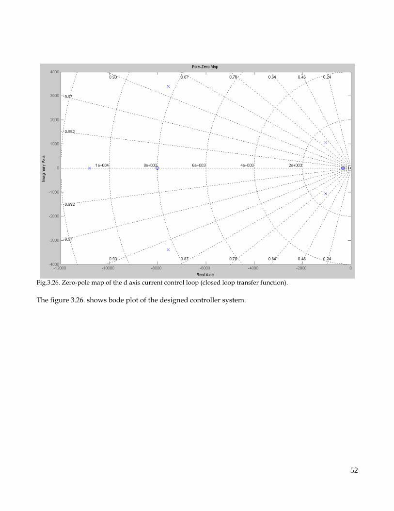
Fig.3.26. Zero-pole map of the d axis current control loop (closed loop transfer function).

The figure 3.26. shows bode plot of the designed controller system.

52

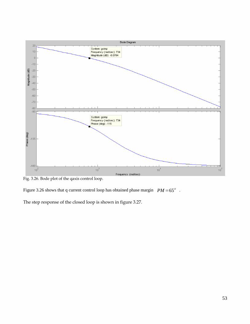
Fig. 3.26. Bode plot of the qaxis control loop.

Figure 3.26 shows that q current control loop has obtained phase margin PM=65o .

The step response of the closed loop is shown in figure 3.27.

53

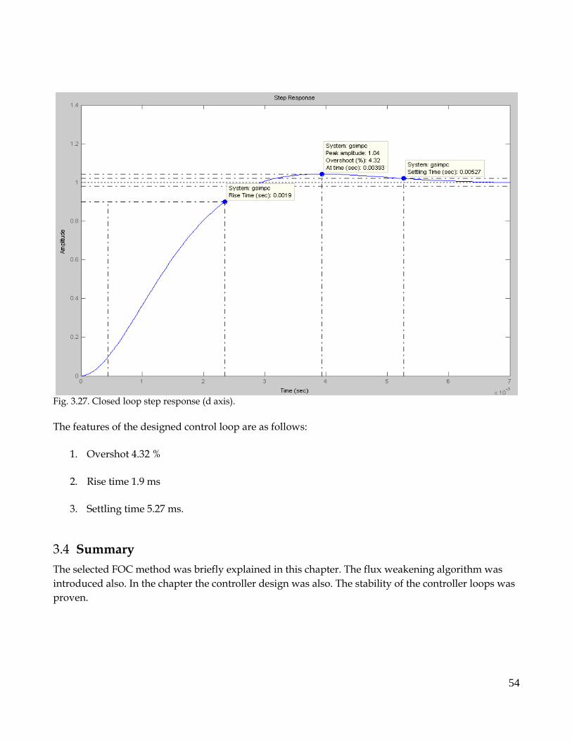
Fig. 3.27. Closed loop step response (d axis).

The features of the designed control loop are as follows:

1. Overshot 4.32 %

2. Rise time 1.9 ms

3. Settling time 5.27 ms.

3.4 Summary

The selected FOC method was briefly explained in this chapter. The flux weakening algorithm was

introduced also. In the chapter the controller design was also. The stability of the controller loops was

proven.

54

55

Chapter 4. Simulations Results and Implementation

In this chapter simulation results are presented and commented. Hardware

implementation is presented and described. The laboratory set-up is

presented and briefly described also.

4.1 Simulations

4.1.1 Method of Testing

The complete generator system including the machine, SVM inverter and the controller has been

investigated and tested using computer simulation. For simulation and analysis purposes the Matlab/

Simulink software was selected.

It is assumed that switches in voltage source converter (VSC) are ideal and no switching

losses are conducted. The IPM machine is modelled in dq reference frame as it was explained

in Chapter 2.

The parameters used are enclosed in Appendix.

The whole system model has been built in continuous environment.

Step load is applied to the DC link voltage to test performance of the simulated generator system.

In the evaluated system, load is presented by 9 brushless permanent magnet motors. Therefore in

simulations the nine step variable load is applied. However the most important test is under the worst

case load conditions (all 9 motors are started in the same moment) and system will be tested under

this conditions. It is assumed that generator is already running at no load mode and then load to the

DC bus is applied. The DC link voltage waveform is crucial in these tests because the bus voltage

should be regulated to remain within voltage band specified due to requirements given by norms.

The system is also tested at high speed condition to verify flux weakening mode controller and the

56

system ability to give constant power regardless input generator speed (within assumed bandwidth).

4.1.2 Obtained Results

System behavior at base speed

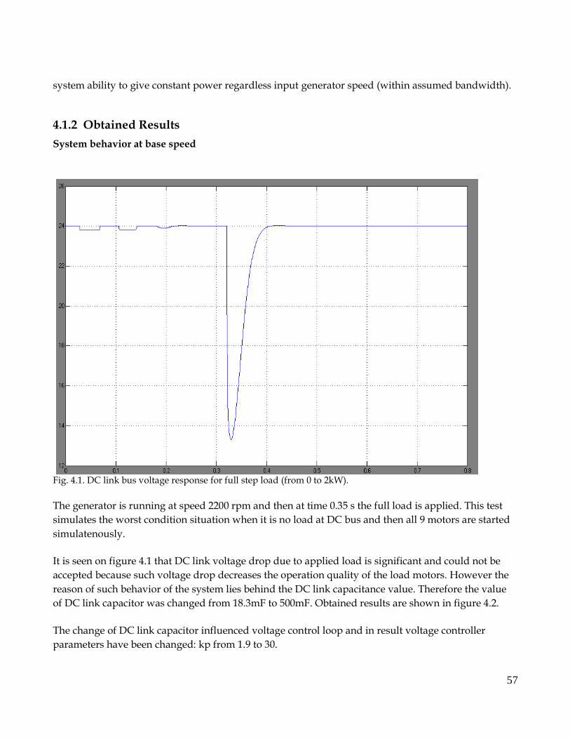
Fig. 4.1. DC link bus voltage response for full step load (from 0 to 2kW).

The generator is running at speed 2200 rpm and then at time 0.35 s the full load is applied. This test

simulates the worst condition situation when it is no load at DC bus and then all 9 motors are started

simulatenously.

It is seen on figure 4.1 that DC link voltage drop due to applied load is significant and could not be

accepted because such voltage drop decreases the operation quality of the load motors. However the

reason of such behavior of the system lies behind the DC link capacitance value. Therefore the value

of DC link capacitor was changed from 18.3mF to 500mF. Obtained results are shown in figure 4.2.

The change of DC link capacitor influenced voltage control loop and in result voltage controller

parameters have been changed: kp from 1.9 to 30.

57

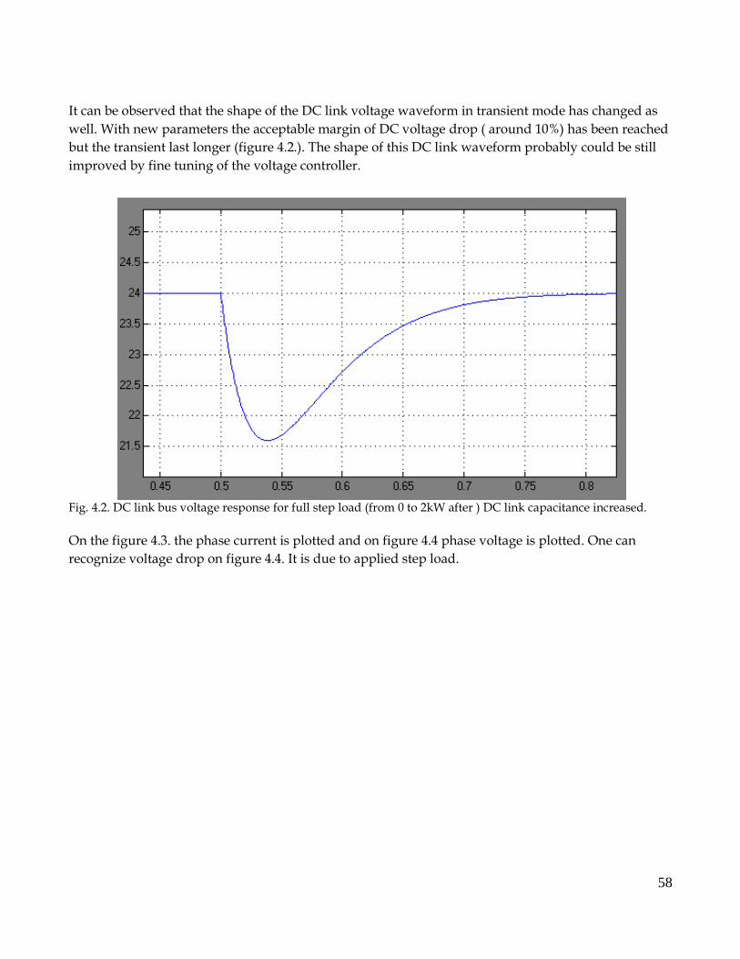
It can be observed that the shape of the DC link voltage waveform in transient mode has changed as

well. With new parameters the acceptable margin of DC voltage drop ( around 10%) has been reached

but the transient last longer (figure 4.2.). The shape of this DC link waveform probably could be still

improved by fine tuning of the voltage controller.

Fig. 4.2. DC link bus voltage response for full step load (from 0 to 2kW after ) DC link capacitance increased.

On the figure 4.3. the phase current is plotted and on figure 4.4 phase voltage is plotted. One can

recognize voltage drop on figure 4.4. It is due to applied step load.

58

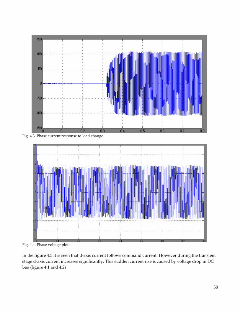
Fig. 4.3. Phase current response to load change.

Fig. 4.4. Phase voltage plot.

In the figure 4.5 it is seen that d-axis current follows command current. However during the transient

stage d-axis current increases significantly. This sudden current rise is caused by voltage drop in DC

bus (figure 4.1 and 4.2)

59

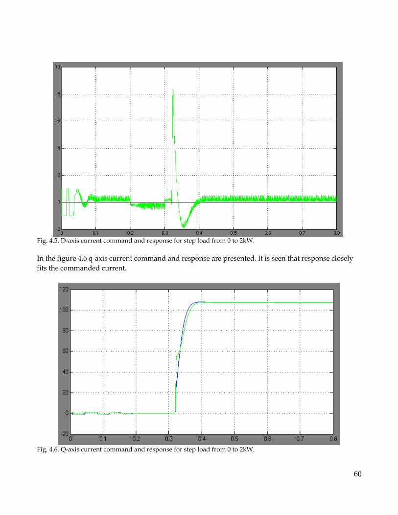
Fig. 4.5. D-axis current command and response for step load from 0 to 2kW.

In the figure 4.6 q-axis current command and response are presented. It is seen that response closely

fits the commanded current.

Fig. 4.6. Q-axis current command and response for step load from 0 to 2kW.

60

4.1.3 Model verification

The accuracy of the controller design methods could be evaluated here. There were three controllers

designed; DC link voltage controller, q-axis current controller and d-axis current controller.

In this chapter system responses to a step load are observed. These results could be compare with

results obtained in Chapter 3. In Chapter 3 controllers were designed using common methods like

symmetry Criterion and Optimum Modulus. In Chapter 3 theoretical responses of the system based

on derived transfer function were calculated. In figures 3.8, 3.17 and 3.24. the system responses to step

signal are presented. These waveforms could be compared with equivalent responses from model

built in Simulink :4.1, 4.5, 4.6.

The plots 3.8 and 4.6 show behavior of the q-axis controller. It can be observed that these plots are

close to each other. Therefore it means that controller parameters were designed in correct way and

simplified transfer function based model has some reflection in the Simulink based system model.

On the figures 3.17 and 4.1 DC link voltage controller behavior is shown. It can be observed that these

waveforms are similar in shape, however this in figure 4.1 seems to be more stiff after transient. It

could be caused by some external factors which were not taken into account during controller design.

Though also it is important to write that voltage controller parameters were changed from values

directly calculated in chapter 3 to obtain better DC link voltage response.

The d-axis current response can be observed in figures 4.5 and 3.24. It can be easily seen that Simulink

model response (figure 4.5) is not so close to the theoretically calculated response in Chapter 3.

It is seen in figure 4.5 that step load introduces quite large overshot. However this

misalingment of these two plots is mainly caused by voltage controller parameters change. In

the result different voltage response forces d-axis current to changed behavior.

4.1.4 Summary

Stability of the control system was tested in continuous domain. The reliability of the control system

also was tested and it was proven that control is accurate. The model comparison was done and

verification process of the models was also performed.

4.2 Implementation

4.2.1 Digital Signal Processor

The tested control algorithm for generator was implemented in TMS320F2812 Digital Signal Processor

61

(DSP).

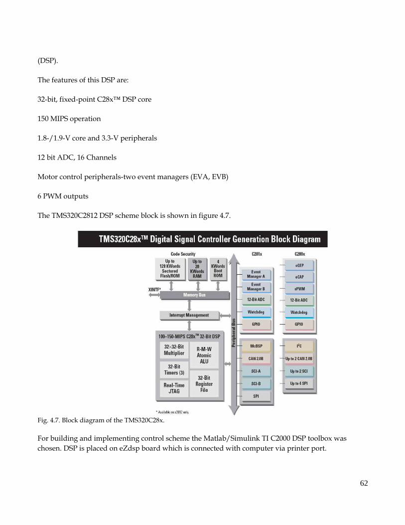
The features of this DSP are:

32-bit, fixed-point C28x™ DSP core

150 MIPS operation

1.8-/1.9-V core and 3.3-V peripherals

12 bit ADC, 16 Channels

Motor control peripherals-two event managers (EVA, EVB)

6 PWM outputs

The TMS320C2812 DSP scheme block is shown in figure 4.7.

Fig. 4.7. Block diagram of the TMS320C28x.

For building and implementing control scheme the Matlab/Simulink TI C2000 DSP toolbox was

chosen. DSP is placed on eZdsp board which is connected with computer via printer port.

62

The control system is built with help of TI C2000 DSP toolbox using specially designed blocks from

DSP library together with generic Simulink blocks. The Simulink builder coverts blocks system to C

code and then it is transferred , with help of the Code Composer Studio program, to the DSP board.

TI C2000 toolbox speeds up implementation process because it has library which contains commonly

used functions in electric drives applications such Clarke and Parke transformations or SVM blocks.

Therefore user is not supposed to writing all control scheme in C code or in Assembler, which is time

consuming process.

For floating point operations the IQmath library was used.

For storing floating point numbers the QN format is used. The native length of the word for 28xx

processor is 32 bit (processor is 32 bit type). The Q format offers compromise between the range and

the precision ( the higher precision the narrower range). The first bit from the left is used as sign

representation. After sign there are integer bits and then the fractional bits. The N number determines

how many bits are used to represent the fractional part of the whole number. Therefore number of the

bits fixed to integer part is determined as 32-1-N [21].

The [20] reported important feature of the PWM timer. During timer underflow the analog to digital

conversion is performed and also rewriting values from shadow registers to working registers is done.

Unfortunately TI C2000 Real Time Workshop tool does not control the shadow register work in

ordered way. Therefore values are written from shadow register to working register both on

underflow and overflow of the PWM timer. It occurs on unpredictable states of PWM- generation of

random reset signals.

To avoid such situation the rewriting process has to be handled only during underflow event. To set

up this process two CLD bits; COMCONA and COMCONB has to be set to 00. It is impossible to do it

in TI C2000 so such changes are made in Code Composer Studio after built code in Matlab and after

project is rebuilt again [20].

4.2.2 Signal Sensing

To gathering signals from controlled object the ADC module is used.

Analog inputs of the ADC are within range 0 to 3 V . However measured sinusoidal signals ( i.e. phase

current) are bipolar and the 1.5 V offset has to be added to the input signal to fulfill 0-3 V requirement

of the ADC input. The signal sensing circuit is shown in figure 4.8. This circuit is put on DSP board

interface.

63

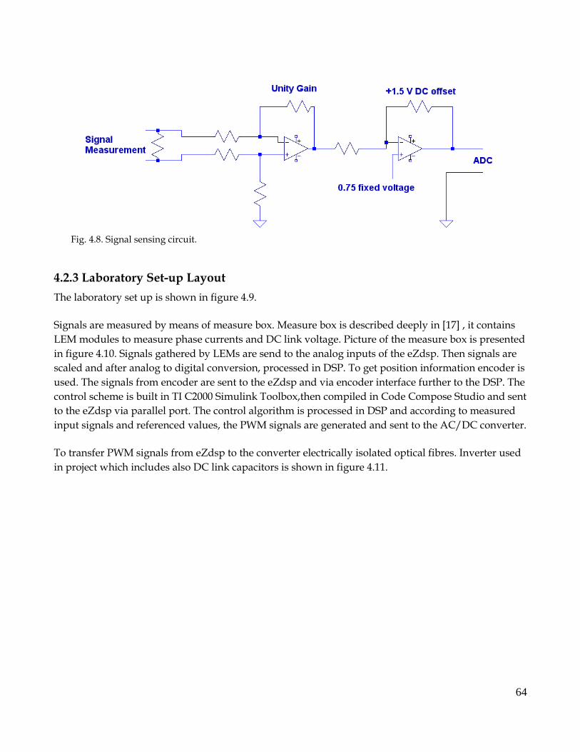
Fig. 4.8. Signal sensing circuit.

4.2.3 Laboratory Set-up Layout

The laboratory set up is shown in figure 4.9.

Signals are measured by means of measure box. Measure box is described deeply in [17] , it contains

LEM modules to measure phase currents and DC link voltage. Picture of the measure box is presented

in figure 4.10. Signals gathered by LEMs are send to the analog inputs of the eZdsp. Then signals are

scaled and after analog to digital conversion, processed in DSP. To get position information encoder is

used. The signals from encoder are sent to the eZdsp and via encoder interface further to the DSP. The

control scheme is built in TI C2000 Simulink Toolbox,then compiled in Code Compose Studio and sent

to the eZdsp via parallel port. The control algorithm is processed in DSP and according to measured

input signals and referenced values, the PWM signals are generated and sent to the AC/DC converter.

To transfer PWM signals from eZdsp to the converter electrically isolated optical fibres. Inverter used

in project which includes also DC link capacitors is shown in figure 4.11.

64

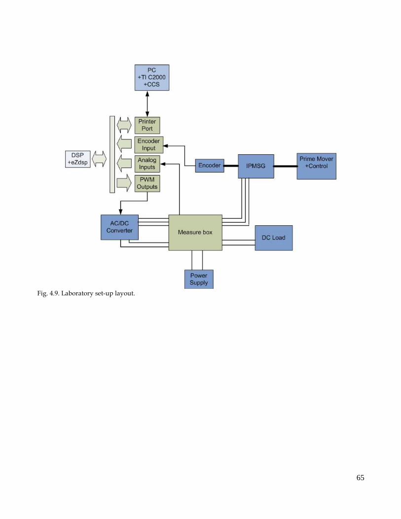
Fig. 4.9. Laboratory set-up layout.

65

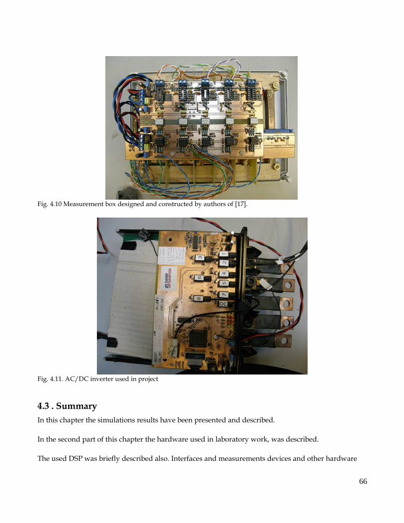
Fig. 4.10 Measurement box designed and constructed by authors of [17].

Fig. 4.11. AC/DC inverter used in project

4.3 . Summary

In this chapter the simulations results have been presented and described.

In the second part of this chapter the hardware used in laboratory work, was described.

The used DSP was briefly described also. Interfaces and measurements devices and other hardware

66

were presented as well.

67

68

Chapter 5. Conclusions and Future Work

5.1 Conlcusions

The presented project work concerns (FOC) of the IPMG which delivers power to the DC link bus.

Regarding this the different AC/DC converters topologies were presented and described. Also several

FOC methods comparison was done. The PWM rectifier topology was selected because it seems to be

most promising and also can handle sophisticated control strategies like FOC scheme.

Mathematical models of the system were derived and presented.

The selected FOC strategy was tested and verified in Matlab/Simulink software . Stable control loop

control method was obtained. It was shown that designed control method fulfill requirements for

robust control scheme for IPM generator.

The selected control strategy was implemented in DSP. The TI C2000 Matlab/Simulink Toolbox was

used to implement control scheme in DSP. The TI C2000 Matlab/Simulink Toolbox decreased time

needed for implementation process.

The laboratory set-up was also presented. DSP used as implementation platform is also described in

the project.

5.2 Future Work

The presented control strategy seems to be a promising option. Therefore further investigating in this

topic could bring beneficial improvements to the considered system. There are several issues in the

project worth to work on:

Sensorless operation of the generator could be introduced. It will reduce the number of sensors

used in the system. This will lead to the higher reliability and lower cost of the whole system.

The system energy consumption could be estimated and then the energy management strategy

could be introduced. It means that energy storage devices can be used and in the result the

system reliability will increase and also power level of the diesel engine/generator system can

be reduced.

The investigation for proper design of the generator could be considered . Together with well

69

designed robust controller it extract full performance capability of the system.

The starting/alternator mode could be also considered because it leads to reduce number of

parts in the propulsion system

70

71

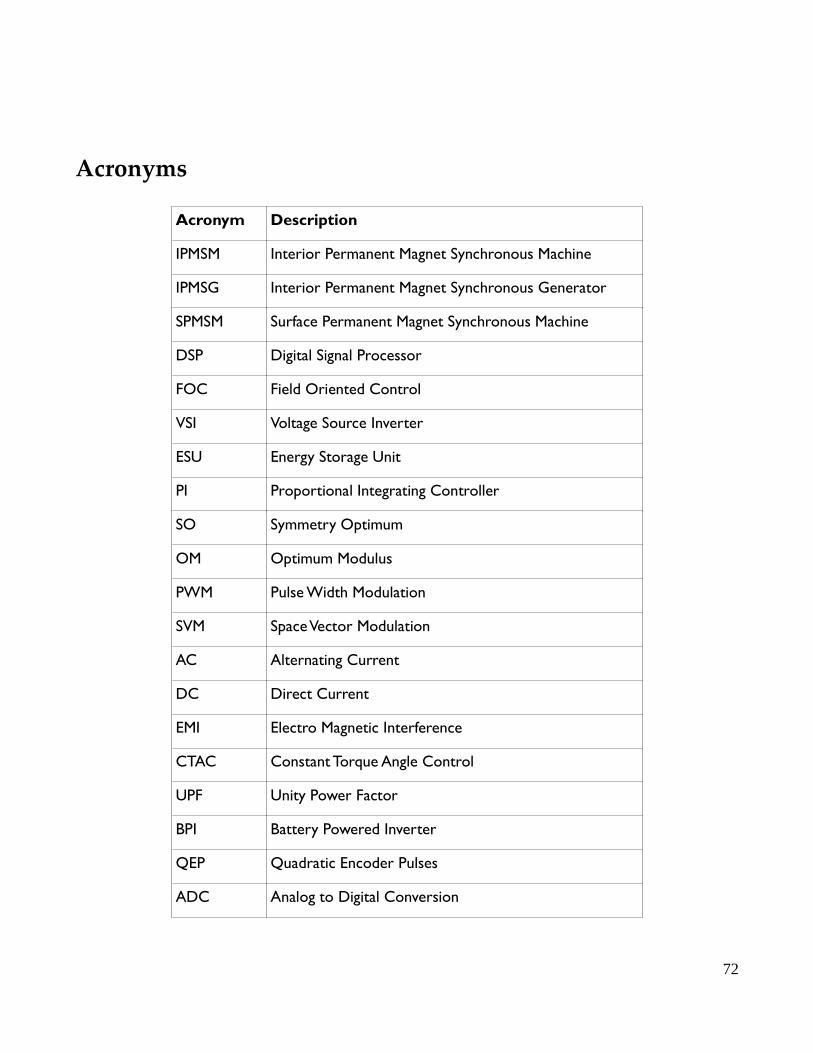
Acronyms

Acronym Description

IPMSM Interior Permanent Magnet Synchronous Machine

IPMSG Interior Permanent Magnet Synchronous Generator

SPMSM Surface Permanent Magnet Synchronous Machine

DSP Digital Signal Processor

FOC Field Oriented Control

VSI Voltage Source Inverter

ESU Energy Storage Unit

PI Proportional Integrating Controller

SO Symmetry Optimum

OM Optimum Modulus

PWM Pulse Width Modulation

SVM Space Vector Modulation

AC Alternating Current

DC Direct Current

EMI Electro Magnetic Interference

CTAC Constant Torque Angle Control

UPF Unity Power Factor

BPI Battery Powered Inverter

QEP Quadratic Encoder Pulses

ADC Analog to Digital Conversion

72

BLDC Brushless DC motor

BEMF Back Electromotive Force

73

74

Nomenclature List

Parameter

Description

R s Stator resistance

L sd Stator inductance in the d-axis

Lsq Stator inductance in the q-axis

i sd Stator d-axis current

i sq Stator q-axis current

fd Permanent magnet flux

m Electrical speed

mech Mechanical speed

T em Electromagnetic torque

T mech Mechanical torque

T L Load Torque

T sd Electrical time constant for d-axis

T sq Electrical time constant for q-axis

V s Stator voltage

I s Stator current

V dc DC link voltage

idc DC link current

m Air gap flux

Factor which determines angle of the current in field weakening mode

75

M Modulation index

v decq Decoupling voltage component in q-axis

v decd Decoupling voltage component in d-axis

T s Sample time

f PWM Switching frequency

76

77

Bibliography

[1] M. P. Kazmierkowski, R. Krishnan, and F. Blaabjerg, Control in Power Electronics. Academic Press,

2002. ISBN 0-12-402772-5. Chapter 11

[2] N. Mohan, Advanced Electric Drives. MNPERE, 2001. ISBN -9715-2920-5.

[3] B. Bose, Modern Power Electronics and AC Drives. Prentice Hall, 2001. ISBN-0-13-016743-6.

[4] Application report SPRA588. Implementation of a Speed Field Oriented Control

of 3-phase PMSM Motor using TMS320F240.Digital Signal Processing Solutions. September 1999.

[5] O. Koerner, J Brand, K. Rechenberg, Energy Efficient Drive System for Diesel Electric Shunting

Locomotive. EPE 2005 Dresden.

[6] M. J. Khan, M. T. Iqbal, SIMPLIFIED MODELING OF RECTIFIER-COUPLED BRUSHLESS DC

GENERATORS.4th International Conference on Electrical and Computer Engineering ICECE 2006,

19-21 December 2006, Dhaka, Bangladesh.

[7] Z. Wang, L. Chang, PWM AC/DC BOOST CONVERTER SYSTEM FOR INDUCTION GENERATOR

IN VARIABLE-SPEED WIND TURBINES.CCECE/CCGEI, Saskatoon, May 2005.

[8] D. M. Whaley, G. Ertasgin, W. L. Soong, N. Ertugrul, J. Darbyshire,

H. Dehbonei, Ch. V. Nayar, Investigation of a Low-Cost Grid-Connected Inverter for Small-Scale Wind

Turbines Based on a Constant-Current Source PM Generator. IEEE 2006.

[9] I. Meny, P. Enrici, J. J. Huselstein, D. Matt, Simulation and testing low power wind system. IEEE 2004.

[10] N. Mohan, First Course Power Electronics and Drives. MNPERE 2003. ISBN- 0-9715292-2-1.

[11] M. P. Kazmierkowski, H. Tunia. Automatic Control of Converter-Fed Drives. ELSEVIER, 1994.

[12] M. Valentini, A. Raducu, T. Ofeigsson, Control of a variable speed variablepitch wind turbinewith full power converter. Aalborg University December 2007.

[13] G. F. Franklin. Feedback Control of Dynamic Systems. Prentice Hall, 2006

[14] F. Jov, A. D. Hansen, P. Soersen, F. Blaabjerg. Wind Turbine Blockset in Matlab/Simulink. General

78

Overview and Description of the Models. Aalborg University, March 2004. ISBN 87-89179-46-3.

[15] P. Perera, D. Chandana, Sensorless Control of Permanent Magnet Synchronous Motor Drives. Institute

of Energy Technology, Aalborg University 2002.

[16] J. Wai, T. M. Jahns, A New Control Technique for Achieving Wide Constant Power Speed Operation with

an Interior PM Alternator Machine. IEEE 2001.

[17] T.N. Matzen, E. Schaltz. Sensorless control of an IPMSM for hydraulic pump application. AalborgUniversity, 2005. Master Project in Power Electronics and Drives.

[19] T. M. Jahns, Flux-Weakening Regime Operation of an Interior Permanent-Magnet Synchronous Motor

Drive. Industrial Application Society Meeting, Denver, CO, September 28-October 3. IEEE 1987.

[18] M. P. Kazmierkowski, R. Krishnan, and F. Blaabjerg, Control in Power Electronics. AcademicPress, 2002. ISBN 0-12-402772-5. Chapter 7,pages 225-242.

[20] R. Ciszewski, Sz. Beczkowski, Evaluation of three-level voltage source PWM inverter topologies.

Aalborg University June 2006.

[21] IQ Math Library A Virtual Floating Point Engine, Module user's guide C28x Foundation Software

[22] P. Vas, Sensorless vector and direct torque control. Oxford Science Publications, 1998. ISBN0-1985-6465-1.

[23] eZdsp F2812 Technical Reference. Digital Development Systems. Spectrum Digital inc.

506265-0001 Rev. F. September 2003.

[24] P. Krause, O. Wasynczuk, and S. Sudhoff, Analysis of Electric Machinery and Drive Systems.

J.Wiley and Sons, 2002. ISBN -0471-1432-6.

[25] Field oriented controf of 3-phase ac-motors, tech. rep., Texas Instruments Europe, February1998.

Literature Number: BPRA073.

79

80

Appendix A

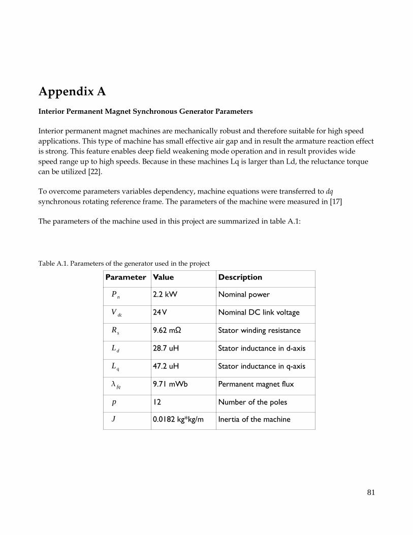
Interior Permanent Magnet Synchronous Generator Parameters

Interior permanent magnet machines are mechanically robust and therefore suitable for high speed

applications. This type of machine has small effective air gap and in result the armature reaction effect

is strong. This feature enables deep field weakening mode operation and in result provides wide

speed range up to high speeds. Because in these machines Lq is larger than Ld, the reluctance torque

can be utilized [22].

To overcome parameters variables dependency, machine equations were transferred to dq

synchronous rotating reference frame. The parameters of the machine were measured in [17]

The parameters of the machine used in this project are summarized in table A.1:

Table A.1. Parameters of the generator used in the project

Parameter Value Description

Pn 2.2 kW Nominal power

V dc 24 V Nominal DC link voltage

R s Ω9.62 m Stator winding resistance

Ld 28.7 uH Stator inductance in d-axis

Lq 47.2 uH Stator inductance in q-axis

fq 9.71 mWb Permanent magnet flux

p 12 Number of the poles

J 0.0182 kg*kg/m Inertia of the machine

81

82

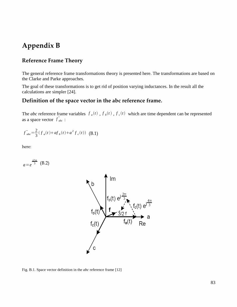
Appendix B

Reference Frame Theory

The general reference frame transformations theory is presented here. The transformations are based onthe Clarke and Parke approaches.

The goal of these transformations is to get rid of position varying inductances. In the result all thecalculations are simpler [24].

Definition of the space vector in the abc reference frame.

The abc reference frame variables f a t , f bt , f c t which are time dependent can be representedas a space vector f abc :

f abc=23 f at af b t a 2 f c t (B.1)

here:

a=ej2

3 (B.2)

Fig. B.1. Space vector definition in the abc reference frame [12]

83

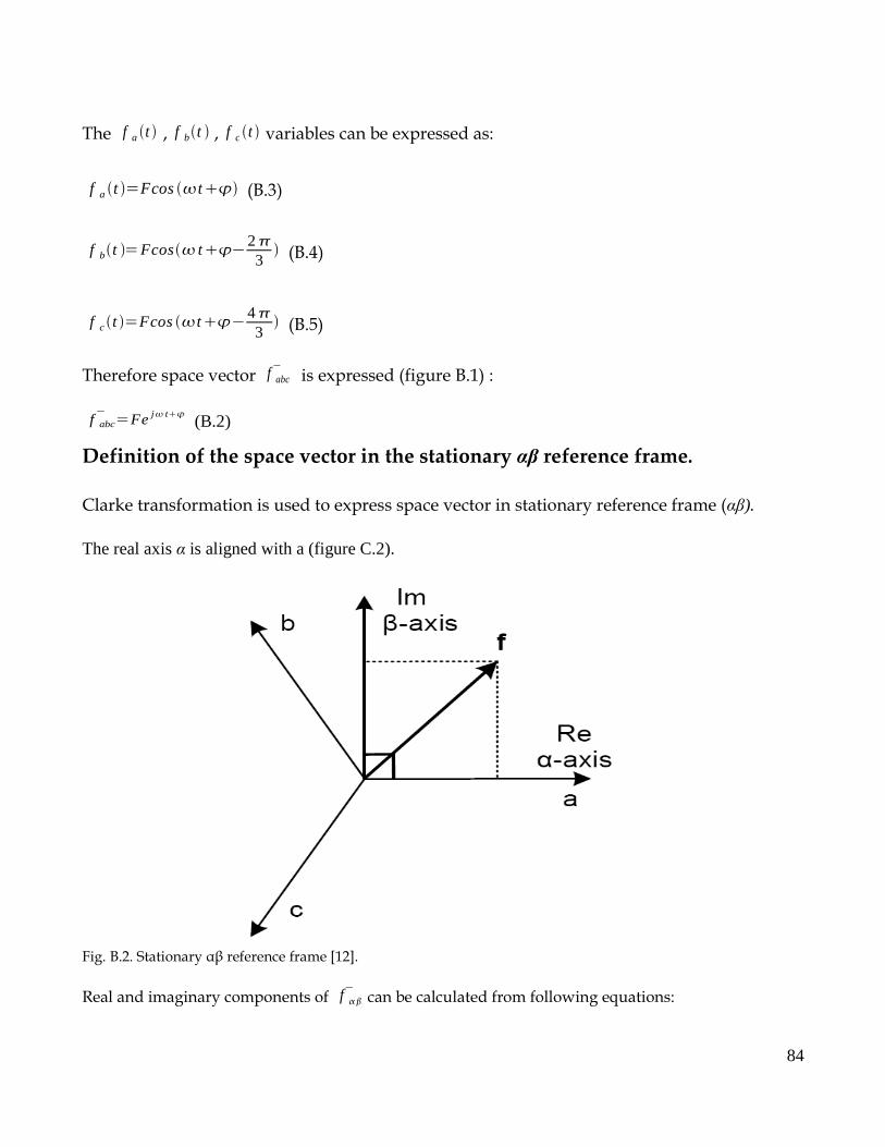
The f a t , f bt , f c t variables can be expressed as:

f a t =Fcos t (B.3)

f bt =Fcos t23

(B.4)

f ct =Fcos t43

(B.5)

Therefore space vector f abc is expressed (figure B.1) :

f abc=Fe j t (B.2)

Definition of the space vector in the stationary αβ reference frame.

Clarke transformation is used to express space vector in stationary reference frame (αβ).

The real axis α is aligned with a (figure C.2).

Fig. B.2. Stationary αβ reference frame [12].

Real and imaginary components of f can be calculated from following equations:

84

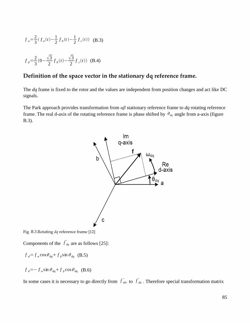
f =23 f a t

12

f b t 12

f ct (B.3)

f =2303

2f b t

32

f ct (B.4)

Definition of the space vector in the stationary dq reference frame.

The dq frame is fixed to the rotor and the values are independent from position changes and act like DCsignals.

The Park approach provides transformation from αβ stationary reference frame to dq rotating referenceframe. The real d-axis of the rotating reference frame is phase shifted by dq angle from a-axis (figureB.3).

Fig. B.3.Rotating dq reference frame [12]

Components of the f dq are as follows [25]:

f d= f cosdq f sin dq (B.5)

f d= f sin dq f cosdq (B.6)

In some cases it is necessary to go directly from f abc to f dq . Therefore special transformation matrix

85

is used to maintain transition [11], [24].

f dq=T dq⋅ f abc (B.7)

T dq=23 [ cosdq cosdq

23

cos dq23

sin dq sin dq23

sin dq23

0.5 0.5 0.5] (B.8)

The inverse transformation f dq to f abc is maintained by inverse transformation matrix:

f abc=T dq1⋅ f dq (B.9)

T dq1=

23 [

cosdq sin dq 1

cos dq23

sin dq23

1

cos dq23

sin dq23

1] (B.10)

86

87

Appendix C

Hardware Set-up

eZdsp F2812 Board

The eZdsp F2812 is specially designed board which allows to examine and evaluate the

TMS320C2812DSP [23].

The eZDsp provides fast code verification. C2000 Tools Code Composer driver reduces complexity of

the developed code. Optionally board has JTAG connector which acts like interface for other

debuggers to provide high level language debug [23].

Features of the eZdsp:

TMS320F2812 Digital Signal Processor

150 MIPS operating speed

18K words on-chip RAM

128K words on-chip Flash memory

64K words off-chip SRAM memory

30 MHz. Clock

2 Expansion Connectors (analog, I/O)

Onboard IEEE 1149.1 JTAG Controller

5-volt only operation with supplied AC adapter

TI F28xx Code Composer Studio tools driver

On board IEEE 1149.1 JTAG emulation connector

88

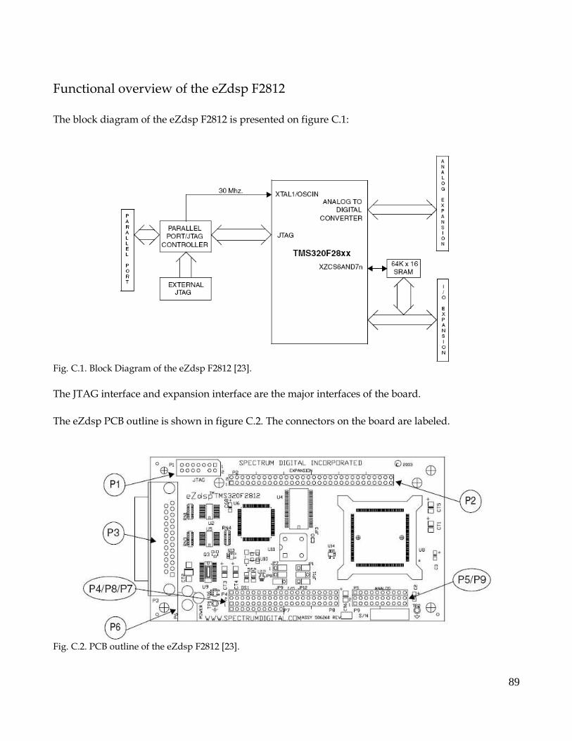
Functional overview of the eZdsp F2812

The block diagram of the eZdsp F2812 is presented on figure C.1:

Fig. C.1. Block Diagram of the eZdsp F2812 [23].

The JTAG interface and expansion interface are the major interfaces of the board.

The eZdsp PCB outline is shown in figure C.2. The connectors on the board are labeled.

Fig. C.2. PCB outline of the eZdsp F2812 [23].

89

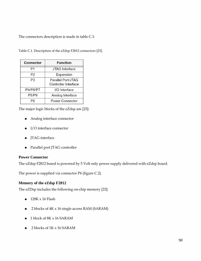
The connectors description is made in table C.1:

Table C.1. Description of the eZdsp F2812 connectors [23].

The major logic blocks of the eZdsp are [23]:

Analog interface connector

I/O interface connector

JTAG interface

Parallel port JTAG controller

Power Connector

The eZdsp F2812 board is powered by 5 Volt only power supply delivered with eZdsp board.

The power is supplied via connector P6 (figure C.2).

Memory of the eZdsp F2812

The eZDsp includes the following on-chip memory [23]:

128K x 16 Flash

2 blocks of 4K x 16 single access RAM (SARAM)

1 block of 8K x 16 SARAM

2 blocks of 1K x 16 SARAM

90

91

Appendix D

Simulation and Implementation Models

In this appendix model built in Matlab/Simulink and used for simulations is presented. Model is

shown in figure D.1.

The system model consist of several components. All these components are described in Chapter 2.

The selected control strategy was implemented in DSP. For implementation process Ti C2000

Simulink Toolbox was used. The figure D.2. Shows model used for implementation in DSP platform:

92

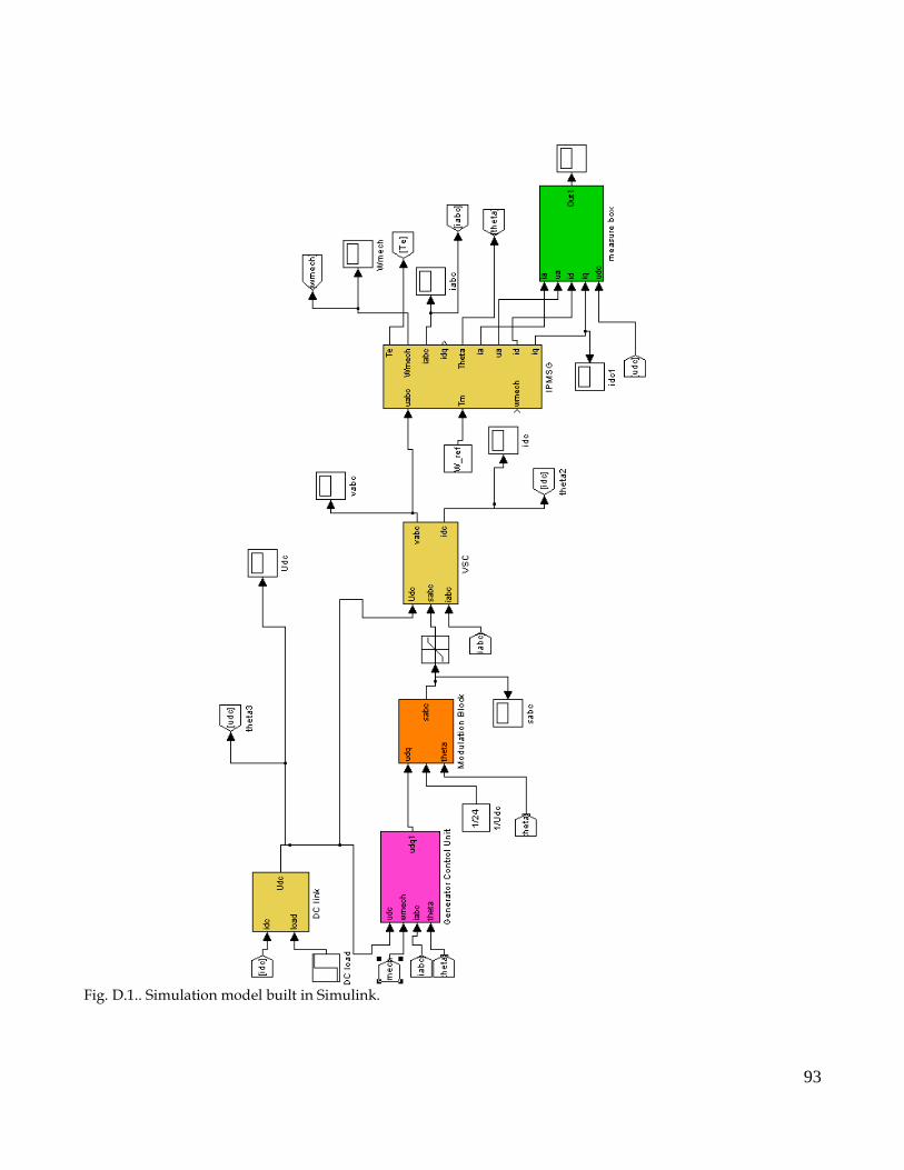
Fig. D.1.. Simulation model built in Simulink.

93

Fig. D.2. Implementation model built in TI C2000 Toolbox

94