UNTREATED MUNICIPAL SEWAGE DISCHARGE IN VICTORIA BIGHT, BRITISH COLUMBIA, CANADA: AN INVESTIGATION OF SEDIMENT METAL

CONTAMINATION AND IMPLICATIONS FOR SUSTA INABLE DEVELOPMENT

by

DUŠAN L. MARKOVIC

B.A., McMaster University, 1995

A thesis submitted in partial fulfillment of the requirements for the degree of

MASTER OF SCIENCE

in ENVIRONMENT AND MANAGEMENT

We accept this thesis as conforming to the required standard

.......................................................... Dr. Ann Dale, MEM Program Manager

Science, Technology & Environment Division

.......................................................... Dr. Matt Dodd, Professor

Science, Technology & Environment Division

.......................................................... Dr. Patrick McLaren, President

GeoSea Consulting (Canada) Ltd.

ROYAL ROADS UNIVERSITY

April, 2003

© Dušan Markovic

2

ACKNOWLEDGMENTS I would like to extend my sincerest thanks to Dr. Patrick McLaren for the incredible

amount of support and time he provided for this project. It truly could not have taken

place without his generosity. I would like to extend the same sincere thanks to Dr. Matt

Dodd who provided excellent guidance throughout the project, was always there when I

needed him, and always had a positive a ttitude – it was greatly appreciated.

I would also like to thank Mr. Bruce Wilmont, Mr. Scot Mackillop and Mr. Jonathan

Francour for their help during the sampling program.

Finally, I would like to thank my wife Jill for supporting me throughout this project.

3

Table of Contents

ABSTRACT...................................................................................................................................8

1.0 INTRODUCTION ...................................................................................................................9

1.1 CRD OUTFALLS ....................................................................................................................9 1.2 HEAVY METALS ...................................................................................................................11 1.3 SEDIMENTS ..........................................................................................................................12 1.4 SUSTAINABLE DEVELOPMENT.............................................................................................13 1.5 SIGNIFICANCE OF RESEARCH .............................................................................................13

2.0 LITERATURE REVIEW......................................................................................................17

2.1 OPPOSING VIEWS................................................................................................................17 2.2 THE SCIENCE.......................................................................................................................18 2.3 OTHER ISSUES....................................................................................................................21

3.0 STUDY AREA: PHYSICAL SETTING.............................................................................21

3.1 QUATERNARY GEOLOGY.....................................................................................................22 3.2 TEMPERATURE AND SALINITY .............................................................................................23 3.3 WIND PATTERNS .................................................................................................................24 3.4 TIDES AND CURRENTS ........................................................................................................24

4.0 FIELD METHODS ...............................................................................................................27

4.1 SAMPLE DESIGN ..................................................................................................................27 4.2 SAMPLE COLLECTION ..........................................................................................................27

4.2.1 Sediment Grain-Size Samples ................................................................................27 4.2.2 Sample Complications..............................................................................................29 4.2.3 Sediment Heavy Metal Samples.............................................................................29

5.0 LABORATORY METHODS...............................................................................................31

5.1 SEDIMENT GRAIN-SIZE ANALYSIS.......................................................................................32 5.1.1 Malvern Mastersizer 2000 Laser Particle Sizer....................................................32 5.1.2 Grain-Size Analysis Technique – Laser Analysis.................................................33 5.1.3 Grain-Size Analysis Technique – Sieve Analysis.................................................35 5.1.4 Grain-Size Data Merging Technique......................................................................35

5.2 HEAVY METALS ANALYSIS ..................................................................................................36 5.2.1 Sample Preparation ..................................................................................................36 5.2.2 Sample Digestion ......................................................................................................37 5.2.3 Flame Atomic Absorption Spectrometry ................................................................37

6.0 RESULTS AND DISCUSSION .........................................................................................39

6.1 SEDIMENTS IN VICTORIA BIGHT ..........................................................................................39 6.1.1 Sediment Type...........................................................................................................39 6.1.2 Fine Sediments ..........................................................................................................41

6.2 DERIVATION OF CONTAMINANT VALUES .............................................................................41 6.2.1 Interpretation of FAA Light Absorbance Values...................................................41 6.2.2 Quality Assurance and Quality Control (QA/QC) .................................................43 6.2.3 Potential Sources of Error ........................................................................................45

4

6.3 SPATIAL AND STATISTICAL ANALYSIS .................................................................................45 6.3.1 Spatial Distribution of Metals...................................................................................45 6.3.2 Statistical Analysis.....................................................................................................51

6.4 SEDIMENT CONTAMINATION AND SUSTAINABLE DEVELOPMENT........................................60 6.4.1 Sustainable Development........................................................................................60 6.4.2 Sediment Quality Guidelines...................................................................................63

7.0 CONCLUSIONS..................................................................................................................69

REFERENCES...........................................................................................................................71

5

LIST OF FIGURES Figure 1 Study Area

Figure 2 CRD Sample/Monitoring Sites

Figure 3 Sample Design

Figure 4 Potential Chemical Survey Sites

Figure 5 Quaternary Geology of Victoria Bight

Figure 6 Wind Patterns in Victoria Bight

Figure 7a Macaulay Point Current Meter Data

Figure 7b Clover Point Current Meter Data

Figure 8 Sample Sites Visited and Hard Ground Stations

Figure 9 Chemical Sites Sampled

Figure 10 Sediment Type Map

Figure 11 Percent Fines Map

Figure 12 Chromium Distribution

Figure 13 Copper Distribution

Figure 14 Zinc Distribution

Figure 15a Chromium vs. Distance

Figure 15b Copper vs. Distance

Figure 15c Zinc vs. Distance

Figure 16a Chromium vs. Direction

Figure 16b Copper vs. Direction

Figure 16c Zinc vs. Direction

Figure 17 Chromium Sediment Quality Guidelines

Figure 18 Copper Sediment Quality Guidelines

Figure 19 Zinc Sediment Quality Guidelines

6

LIST OF TABLES and APPENDICES Table 1 Sediment Data Percent Similar

Table 2 Grain-Size Scales for Sediments

Table 3 Summary of Sediment Types

Table 4 Method Blank Values

Table 5 Duplicate RPD Values

Table 6 Descriptive Statistics

Table 7 Correlation Between Metals and % Fines

Table 8 Correlation Between Metals and Distance

Table 9 Number of Observations per Direction

Table 10 Correlation Between Log Transformed Metals

Table 11 Data Suitability Test: Log Metals

Table 12 Total Variance Explained: Log Metals

Table 13 Extracted Components: Log Metals

Table 14 Correlation Between Normalized Log Metals

Table 15 Data Suitability Test: Normalized Log Metals

Table 16 Total Variance Explained: Normalized Log Metals

Table 17 Extracted Components: Normalized Log Metals

Table 18 CRD/WDOE Sediment Quality Guidelines

Appendix 1 – Grain-Size Data (provided separately) Table A-1 Sediment Grain-Size Data Appendix 2 – Analyte Data (provided separately) Table A-2 Sample Preparation for Chemical Analysis

Table A-3 FAA Light Absorbance Values

Table A-4 Calculation of Chemical Concentrations

Table A-5 Corrected Chemical Concentrations

Table A-6 Chemical Sample Attributes

7

ACRONYMS AET Apparent Effects Threshold ANZECC Australia and New Zealand Environment and Conservation Council BDL Below Detection Limit CCME Canadian Council of Ministers of the Environment Cr Chromium CRD Capital Regional District Cu Copper (D)GPS (Differential) Global Positioning System EC Environment Canada ERL Effects Range Low ERM Effect Range Median ESRI Environmental Systems Research Institute FAA Flame Atomic Absorption GIS Geographic Information System HK Hong Kong ISQG Interim Sediment Quality Guideline ISQV Interim Sediment Quality Value KMO Kaiser-Meyer-Olkin LEL Lowest Effect Level LWMP Liquid Waste Management Plan MET Minimum Effect Threshold MMAG Marine Monitoring Advisory Group MT Metallothionein NAD 83 North American Datum 1983 Ni Nickel NOAA National Oceanic and Atmospheric Administration PC Principal Component PCA Principal Component Analysis PEC Probable Effect Concentration PEL Probable Effect Level RPD Relative Percent Difference SD Sustainable Development SEL Severe Effect Level SLFD Sierra Legal Defence Fund SQG Sediment Quality Guidelines SQO Sediment Quality Objectives TEC Threshold Effect Concentration TEL Threshold Effect Level TET Toxic Effect Threshold US EPA United States Environmental Protection Agency UTM Universal Transverse Mercator WDOE Washington Department of Ecology Zn Zinc

8

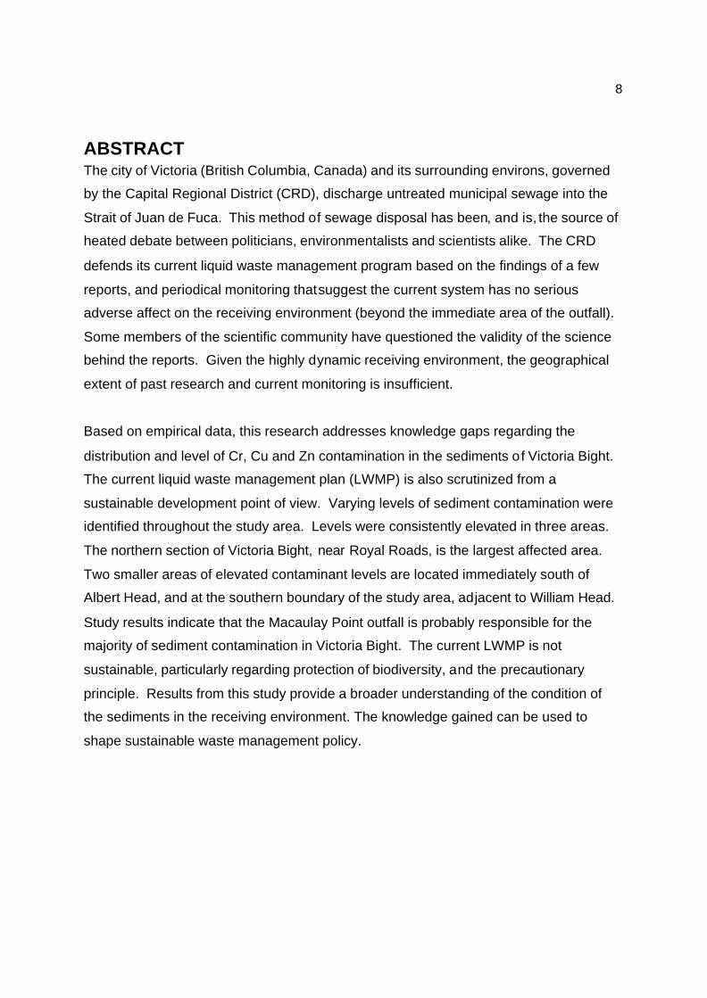
ABSTRACT The city of Victoria (British Columbia, Canada) and its surrounding environs, governed

by the Capital Regional District (CRD), discharge untreated municipal sewage into the

Strait of Juan de Fuca. This method of sewage disposal has been, and is, the source of

heated debate between politicians, environmentalists and scientists alike. The CRD

defends its current liquid waste management program based on the findings of a few

reports, and periodical monitoring that suggest the current system has no serious

adverse affect on the receiving environment (beyond the immediate area of the outfall).

Some members of the scientific community have questioned the validity of the science

behind the reports. Given the highly dynamic receiving environment, the geographical

extent of past research and current monitoring is insufficient.

Based on empirical data, this research addresses knowledge gaps regarding the

distribution and level of Cr, Cu and Zn contamination in the sediments of Victoria Bight.

The current liquid waste management plan (LWMP) is also scrutinized from a

sustainable development point of view. Varying levels of sediment contamination were

identified throughout the study area. Levels were consistently elevated in three areas.

The northern section of Victoria Bight, near Royal Roads, is the largest affected area.

Two smaller areas of elevated contaminant levels are located immediately south of

Albert Head, and at the southern boundary of the study area, adjacent to William Head.

Study results indicate that the Macaulay Point outfall is probably responsible for the

majority of sediment contamination in Victoria Bight. The current LWMP is not

sustainable, particularly regarding protection of biodiversity, and the precautionary

principle. Results from this study provide a broader understanding of the condition of

the sediments in the receiving environment. The knowledge gained can be used to

shape sustainable waste management policy.

9

1.0 Introduction The Greater Victoria area (British Columbia, Canada), governed by the Capital Regional

District (CRD) discharges approximately 120,000m3 of untreated municipal sewage per

day into the Juan de Fuca Strait through two submarine outfalls located at the southern

tip of Vancouver Island (Figure 1) (CRD, 2000). The aim of the research described in

this paper is to determine the spatial distribution and concentration of selected heavy

metals in surface sediments in Victoria Bight; and to determine if the submarine outfalls

are the likely sources of those metals. This research is the first study to conduct a

thorough sediment survey encompassing all of Victoria Bight to determine the potential

impacts of the outfalls on sediments in the receiving environment. The research

findings are also used to assess the CRD’s current Liquid Waste Management Plan

(LWMP), and the implications for the receiving environment from a sustainable

development perspective.

1.1 CRD Outfalls The CRD sewage outfalls serve a population of approximately 322,000 (SLDF, 1999).

The outfall pipes extend into Victoria Bight from Macaulay Point and Clover Point. The

Macaulay Point outfall is 900mm in diameter and extends 1.7 kilometres into Victoria

Bight terminating in 60m of water. The Macaulay Point outfall serves the municipalities

of Colwood, Esquimalt, View Royal, Langford, Vic West and most of Saanich. Leachate

from the Hartland landfill is also pumped out through the Macaulay Point outfall. In

1999, the average daily discharge from Macaulay Point was 48,500m3. The Clover

Point outfall is 1100mm in diameter and extends 1.1 kilometres into Victoria Bight where

it terminates in 67m of water. The Clover Point outfall serves Victoria, Oak Bay and

Cadboro Bay. The 1999 daily discharge average was 71,800m3. The only treatment

prior to discharge from either outfall is screening through a 6mm mesh to remove large

particles. Screenings are removed twice a week and disposed of at the Hartland

Landfill (CRD, 2000). The effluent discharged into the Strait is the combined liquid

waste from individual households, industries, businesses, institutions, commercial

establishments and landfill leachate (CRD, 2000; SLDF, 1999).

10

Figure 1. Study Area

11

1.2 Heavy Metals The untreated sewage contains a wide variety of chemicals and contaminants that are

potentially harmful to the receiving environment. Some of the contaminants found in

untreated sewage are: polycyclic aromatic hydrocarbons (PAHs), phenols, chlorinated

hydrocarbons, pathogens, polychlorinated biphenyls (PCBs) and heavy metals (SLDF,

1999). This study focuses on heavy metal contamination. The potential harm caused

by heavy metals in the environment has been well documented. Negative effects

observed in a number of organisms range from behavioural changes to death (Rainbow

and Furness, 1990; Langston, 1990; EVS, 1992b; Anderlini and Wear, 1992; Power and

Chapman, 1992). Also, metals are a good indicator of anthropogenic, as opposed to

natural, sources o f contamination (Birch, 1996; Luoma, 1990; Paetzel et al., 2002;

Chague-Goff and Rosen, 2001; Zhang et al., 2001; Sutherland, 2000; Emmerson et al.,

1997; Simeonov et al., 2000).

The three metals analyzed for this study are Chromium (Cr), Copper (Cu) and Zinc (Zn).

The CRD and the U.S. EPA have identified all three metals as priority pollutants (CRD,

2000; Langston, 1990). Of the three metals analyzed, Cu is of prime importance. Past

research indicates that Cu is potentially the most significant marine environmental

pollutant. Studies have shown that Cu may be toxic to biota at levels only marginally

above background levels (Langston, 1990). Also, of particular relevance to this study,

Cu levels in sediments are monitored by the Marine Monitoring Advisory Group

(MMAG), an independent body that monitors and advises the CRD on issues related to

the CRD’s LWMP. Sediment Cu levels are one of the MMAG’s ‘trigger’ mechanisms

that are meant to invoke re-evaluation of the current level of sewage treatment (CRD,

2000; Bright, D. Pers. Comm., 2002). All three metals studied for this project are

routinely analyzed in the determination of sediment contamination (Paetzel et al., 2002;

Sanudo-Wilhelmy et al., 2002; Spencer, 2002; Birch et al., 2001; Chague-Goff and

Rosen, 2001; Zhang et al., 2001; Simeonov et al., 2000; Sutherland, 2000; Ruiz et al.,

1998; Emmerson et al., 1997; Padmalal et al., 1997; Birch, 1996; Huang et al., 1994;

Turner and Millward, 1994; EVS, 1992b).

12

1.3 Sediments Sediments are a matrix of materials usually found beneath bodies of water. They are

composed of inorganic and organic particles made up of shell and rock fragments,

minerals, atmospheric fall-out and eroded soil and waste particles (Power and

Chapman, 1992). Through both natural (e.g. watershed drainage) and un-natural (e.g.

sewage discharge) processes, sediments are ultimately the terminus for both natural

and anthropogenic materials, for which reason they tend to be susceptible to

contamination (Power and Chapman, 1992). In broad terms, sediments can be

classified as either coarse or fine. The coarse fraction (greater than 62µm) is comprised

mainly of stable, non-cohesive inorganic silicate materials. Generally, coarse sediments

are not associated with chemical contamination (Power and Chapman, 1992). The fine

fraction (less than 62µm) consists of particles that have large surface area to volume

ratios. The surfaces of fine particles often carry an electric charge, making fine

sediments more chemically and biologically reactive than coarse sediments, thereby

increasing the likelihood of sorption and desorption (Power and Chapman, 1992). As a

consequence of the physio-chemical properties of fine particles, chemical contamination

is usually associated with fine sediments, a characteristic frequently associated with

depositional areas (Zhang et al., 2001; Padmalal et al., 1997; Power and Chapman,

1992, McLaren and Little, 1987; Young et al., 1985).

The reactive nature of fine particles has serious implications for the fate and transport of

heavy metals in the marine environment. Metals are highly reactive with particles, and

the combined reactivity of fine sediments and heavy metals means that, through

adsorption, sediments trap large portions of incoming contaminants. Sediment metal

concentrations often exceed those in overlying water by several orders of magnitude

(Langston, 1990). As a contaminant sink, sediments are critically important as a direct

source of metal toxins for benthic organisms in marine environments (Luoma, 1990;

Langston, 1990). In regard to environmental monitoring, metal concentrations in

sediments are useful in the assessment of anthropogenic inputs of metals. As such,

sediments provide a good indication of the effects of sewage on receiving environments

(Langston, 1990; Taylor et al., 1998).

13

1.4 Sustainable Development In addition to determining the level and distribution of sediment metal contamination,

this study critically evaluates the science and sediment quality guidelines, used by the

CRD, to assess the state of the receiving environment from a sustainable development

perspective. Actions, activities and systems must adhere to a number of fundamental

principles that underlie sustainable development, to be considered sustainable. The

protection and preservation of biodiversity, and the precautionary principle are two of

the paradigms underlying sustainable development that are particularly relevant to the

issue of sewage disposal to the marine environment. Sediments are a key component

of the marine environment. The organisms that live in and depend on sediments make

up a large portion of the foundation of the marine food chain (Power and Chapman,

1992). Numerous studies have demonstrated that toxic sediments have been the cause

of reductions in, or alterations to, sedimentary organisms (EVS, 1992b; Anderlini and

Wear, 1992; Langston, 1990). Some of the negative impacts these changes to the

marine environment have had on higher trophic levels (including humans) have been

documented. Nevertheless, the long-term effects remain uncertain, and future

generations may be subject to unknown risks (Luoma, 1990).

The loss of a keystone species will eventually lead to a multitude of linked

extinctions through a ripple effect that spreads throughout the ecosystem.

Meyers, N. (as cited in Dale, 2001)

1.5 Significance of Research There have been a limited number of studies regarding the impact of the CRD outfalls

on the sediments in the receiving environment. With the exception of this study, all

previous investigations have been largely confined within a 2km radius of the outfalls.

The most comprehensive study to date is based on 25 sample sites. Of these sites; 12

are within a 1.6km radius of Macaulay Point, 1 site is located 3km southwest of

Macaulay Point, 9 samples are within 1.2km of Clover Point (from which no sediment

was successfully retrieved), and the remaining 3 samples are reference sites located in

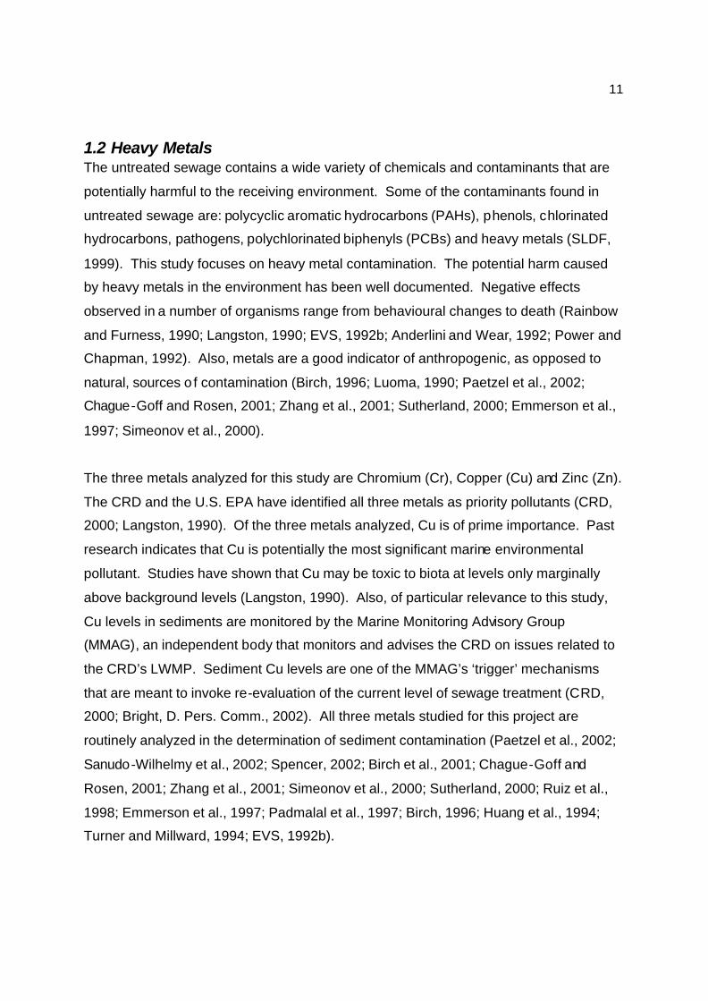
Parry Bay, approximately 10km southwest of the Macaulay Point outfall (Figure 2). The

limited areal extent of previous studies does not satisfactorily address one of the

14

principles of contaminated sediment transport and deposition. It is well understood that

in coastal zones, regardless of the point of introduction, fine particles seek preferred

zones of deposition. In cases of continuous contaminant input, the source of input is

likely to be responsible for consistent contamination at the input site as well as

secondary contamination in depositional areas. Proper surveillance or monitoring

studies must be designed to account for the physical transport of sediments and the

resultant redistribution of their associated contaminants (Luoma, 1990; McLaren and

Little, 1987; Young et al., 1985).

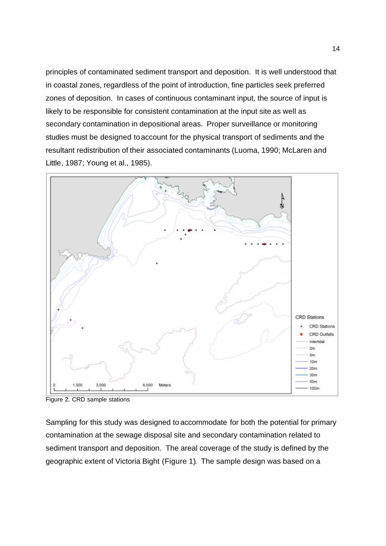
Figure 2. CRD sample stations

Sampling for this study was designed to accommodate for both the potential for primary

contamination at the sewage disposal site and secondary contamination related to

sediment transport and deposition. The areal coverage of the study is defined by the

geographic extent of Victoria Bight (Figure 1). The sample design was based on a

15

hexagonal grid with a 500m resolution. A total of 582 samples sites were initially

identified (Figure 3).

Figure 3. Sample design

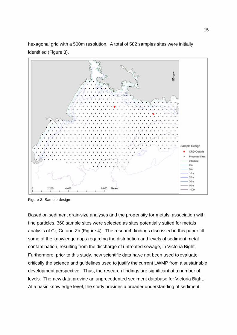
Based on sediment grain-size analyses and the propensity for metals’ association with

fine particles, 360 sample sites were selected as sites potentially suited for metals

analysis of Cr, Cu and Zn (Figure 4). The research findings discussed in this paper fill

some of the knowledge gaps regarding the distribution and levels of sediment metal

contamination, resulting from the discharge of untreated sewage, in Victoria Bight.

Furthermore, prior to this study, new scientific data have not been used to evaluate

critically the science and guidelines used to justify the current LWMP from a sustainable

development perspective. Thus, the research findings are significant at a number of

levels. The new data provide an unprecedented sediment database for Victoria Bight.

At a basic knowledge level, the study provides a broader understanding of sediment

16

types and metal contamination in the receiving environment. This information is an

integral component of rational coastal zone management practices. At a decision

making level, the scientific findings will allow decision makers to make the best use of

the limited resources at their disposal. Finally, the information acquired will allow the

CRD to re-evaluate the current LWMP from a sustainable development perspective.

Doing so would ensure that sound, defendable and most importantly, sustainable liquid

waste management practices are employed by the CRD.

Figure 4. Potential chemical analysis sites

17

2.0 Literature Review

2.1 Opposing Views The CRD’s current LWMP, and the impact of the sewage outfalls on the receiving

environment, has been a continuous source of debate for scientists, environmentalists,

citizens and politicians from all levels of government. The sewage issue is not only an

environmental one, but rather has significant economic and political implications, and

this is evident in scientific literature, outspoken environmental groups, and popular

journalism. As with all contentious issues, there are two sides to the Victoria sewage

debate. Proponents of the status quo argue that the assimilative capabilities of the

receiving environment are more than adequate in terms of handling the volume of waste

discharged. They maintain that the receiving environment is highly dynamic, and that

rapid dilution of waste prevents any build -up of contaminants (Palmer, 1999; Taylor et

al., 1998; Rogers, 1995; EVS, 1992b).

Those who oppose the status quo argue that contamination from the outfalls is

responsible for the closure of a shellfish fishery in the Juan de Fuca Strait, and that the

CRD is in contravention of both the Canadian Fisheries Act, and conditions stipulated in

the CRD’s provincial waste discharge permits. Opponents also claim that negative

impacts to the receiving environment are occurring well beyond the outfalls themselves,

and that the science behind the decision-making is suspect (Cleverley, 2001; Connelly,

1999; SLDF, 1999; Werring, 1999). The published literature surrounding the CRD’s

LWMP reflects both sides of the waste issue. The published literature put forth by

proponents of the current LWMP is comprised of technical and scientific reports along

with peer-reviewed journal articles. There are also a number of informative documents

made available to the public, by the CRD, regarding the LWMP. In contrast, the

majority of the published literature by critics of the CRD’s LWMP is in the form of

newspaper articles, media-releases and reports from environmental groups.

18

2.2 The Science In 1992, in an attempt to reduce the amount of uncertainty regarding the impact of the

outfalls, and placate opponents of the LWMP, the CRD commissioned EVS Consultants

to conduct an environmental assessment on the effects of untreated municipal sewage

on the sediments in the receiving environment. The ensuing report: Sediment and

Related Investigations off the Macaulay and Clover Point Sewage Outfalls (EVS, 1992b)

has been the main source of scientific information for the public and decision-makers

alike. The report and its findings have also been the basis for a number of related

journal articles (Palmer 1999; Taylor et al., 1998; Rogers, 1995), all of which were

authored by either EVS or CRD personnel. The CRD have used the findings of the EVS

report for continued defence of the current LWMP.

The environmental assessment carried out by EVS was conducted in two phases. An

initial study was undertaken to evaluate qualitatively the condition of the receiving

environment (EVS, 1992a). An underwater camera was used to obtain a number of

sediment profile images in the vicinity of the outfalls. These images were used to

identify sites most likely to be impacted from the sewage, and consequently the sites

that would best warrant quantitative analysis and monitoring (EVS, 1992a). With the

exception of potential reference sites in Parry Bay and east of Trial Isla nds, the area

surveyed for outfall monitoring stations was confined to within a 2km radius of each

outfall. While the area investigated addresses the issue of primary contamination at the

site of discharge, it fails to address the issue of secondary contamination associated

with sediment transport. As noted in Section 1.5, regardless of the point of introduction,

fine particles and associated contaminants seek preferred zones of deposition.

Therefore, depositional areas prone to contaminant build-up must be accounted for in

the design of effective surveillance and monitoring programs (Luoma, 1990; McLaren

and Little, 1987; Young et al., 1985).

Having identified monitoring sites, EVS proceeded with the second phase of the

assessment. Sediment samples were collected from Macaulay Point and Parry Bay

stations. Mussels (Modiolus) were collected for tissue analysis, from the Clover Point

19

stations, where no sediment could be retrieved (Figure 2). EVS conducted thorough

analyses of the data they had collected. Rigorous testing for organic and inorganic

contaminants, along with toxicity testing was carried out. The report concluded that the

sewage had minimal impact on the receiving environment, and that those impacts are

confined to within 400m of the Macaulay Point outfall (Taylor et al., 1998; EVS, 1992b).

The findings of the report are questionable for a number of reasons. The initial problem

of failing to address areas of secondary contamination was not rectified in the final

study. This is somewhat surprising considering the main argument used by proponents

to defend the current LWMP; namely, that the receiving environment is highly dynamic

and rapid dilution of the effluent prevents contamination build-up. This is especially

evident near the Clover Point outfall where strong currents have left a scoured seabed

more or less devoid of sediment. Supporters of the status quo also note that the

effluent, which is comprised mainly of fresh water, is more buoyant than the receiving

waters. Therefore, the effluent rises in the water column and is rapidly dispersed before

particulates and associated contaminants settle into the sediments. Related to this, a

drift card study by Crone et al. (1998) indicated that 60% of floatables from the outfalls

remained in Victoria Bight due to tidal currents and eddies. These particular

characteristics suggest that secondary contamination could potentially be more

significant than primary contamination at the source. Despite this, the CRD’s monitoring

sites are concentrated around the outfalls themselves, and the area within 100m of

each outfall is considered the ‘worst case scenario’ (Taylor et al., 1998; EVS, 1992b).

Review of the EVS report leads to other concerns particularly regarding the sample

design used by EVS to conduct the environmental assessment. Three sites in Parry

Bay were used as reference stations (Figure 2). Modelling by Seaconsult in 1992,

however, concluded that deposition from the outfalls is occurring in Parry Bay and south

of William Head (EVS, 1992b). Therefore, although reference sites are normally meant

to provide an example of an undisturbed case, those selected by EVS are likely

contaminated, and consequently are unsuitable (Werring, J. Pers. Comm., 2003).

Furthermore , the EVS sample design was based on an understanding of major currents,

20

transport modelling and underwater photography (EVS, 1992b). There is a line of

sample stations extending southwest from the Macaulay Point outfall, however there are

no samples extending southeast from the outfall, the direction of the most frequent

subsurface current direction (Figure 7a). Sediment transport studies conducted by

GeoSea Consulting further support this, indicating sediment transport in a southeastern

direction from the outfall (GeoSea, 1999).

Another issue to consider when interpreting the findings of the EVS report, and

statements made by the CRD regarding the level and extent of impacts, are the

sediment quality guidelines (SQGs) by which the sediments are being evaluated. The

term ‘contamination’ is highly subjective. Understanding how it has been defined in any

particular situation is crucial in order to put statements regarding contamination into

context. The sediment quality guidelines currently used by the CRD are based on

Apparent Effects Threshold (AET) values originally developed for Puget Sound. These

SQGs were selected because of Victoria’s proximity to Puget Sound, which raises some

questions in terms of their validity (EVS, 1992b). AETs are empirically based and are

site specific (Burton, 2002). Although Victoria is close to Puget Sound, the two

environments are completely different. Puget Sound is a dead-end fiord with a number

of major sediment input sources such as rivers, streams and coastal erosion. The area

is not very dynamic and large depositional areas are expected. Alternatively Victoria

Bight is subject to the full tides and currents of the Pacific Ocean, and is generally a

much more dynamic environment (McLaren, P. Pers. Comm., 2003). Therefore, it is

unlikely that SQGs developed for Puget Sound are a good measure of sediment quality

in Victoria Bight. Furthermore, AETs are defined as the amount of contaminant in

sediments above which a particular effect has always been observed. In the case of

Puget Sound, the effects tested for were acute or chronic adverse effects on aquatic

organisms, or a significant risk to human health (Ginn and Pastorok, 1992). A concern

with AETs is that they are often under-protective since they are founded on levels that

“always” have an effect (Burton, 2002). The SQGs currently used by the CRD are

consistently higher than those developed by British Columbia Environment,

Environment Canada, and the Canadian Council of Ministers of the Environment.

21

2.3 Other Issues Review of the published literature regarding the Victoria sewage outfalls reveals a

number of issues which must be considered when evaluating the situation. As noted

above, all peer reviewed journal articles are based on the EVS report, and written by

CRD or EVS personnel. As a result, any shortcomings from the EVS report, or biases

from supporters of the status quo, have been propagated throughout the literature, and

on to decision-makers and the public.

Negative impacts related to the outfalls are consistently downplayed in the EVS report

and in any CRD literature regarding the outfalls. Impacts are consistently described as

‘minimal’, and the potential importance of sub-lethal effects are downplayed. For

example, the report notes that biomass is greatly increased around the outfalls,

specifically the presence of annelids, yet biodiversity is decreased. The report fails to

mention that this scenario may be an indication of a highly stressed or polluted

environment (Langston, 1990). The report also notes that organisms around the outfall

do not appear affected, yet fails to discuss that the community structure is formed of

tolerant species, and not those normally found in undisturbed environments similar to

Victoria Bight (Anderlini and Wear, 1992).

Politics and economics are obviously an influence on the sewage debate. In 1992, the

CRD held a referendum to determine what level of treatment should be applied to

Victoria’s sewage. The scientific information provided to the public was based on the

EVS report and, according to information in a prosecution brief by the SLDF, the CRD

greatly exaggerated the cost of implementing sewage treatment. Essentially, the public

was told that the sewage is not a problem, and that treating it is prohibitively expensive.

As a result, the public voted to continue with the status quo (Werring and Chapman,

1999).

3.0 Study Area: Physical Setting Victoria, British Columbia, is a coastal city located at the southern tip of Vancouver

Island. The coastline of the Greater Victoria area forms a natural bend, resulting in an

open bay or bight – in this case, Victoria Bight. The geographic extent of Victoria Bight

22

delineates the study area for the research discussed in this paper. Victoria Bight is part

of a larger body of water called the Juan de Fuca Strait. The Juan de Fuca Strait is a

long submarine valley that is the main body of water connecting the Pacific Ocean and

the inner shelf waters of southern British Columbia (Figure 1) (Thomson, 1981).

3.1 Quaternary Geology Juan de Fuca Strait was occupied by continental ice on a number of occasions during

the Pleistocene. The result was the deposition of a number of glacial and inter-glacial

deposits. Studies of the surface geology in the Juan de Fuca Strait indicate that the

deposits are characteristic of a rapid glacial retreat, followed by a rapid change in sea

level (Hewitt and Mosher, 2001). Four main surficial geological units have been

identified in recent investigations by Hewitt and Mosher (2001). Unit 1 is bedrock, made

up primarily of Cretaceous and Tertiary sedimentary rocks. Unit 2 consists of ice

contact sediments such as till or diamicton. Unit 3 is comprised of glacial-marine

deposits and Unit 4, composed of two sub -units, is identified as post-glacial sediments.

The majority of Victoria Bight is classified as post-glacial (Unit 4a). These are organic-

rich sandy-mud sediments with shell fragments. There are bedrock (Unit 1) outcrops at

Albert Head and William Head. Constance Bank is composed mainly of glacial marine

till (Unit 2). Just north of Constance Bank there is a field of sand waves , an indication

that sediments are actively being transported. The eastern side of Victoria Bight (in the

vicinity of Clover Point) is dominated by coarse pebbles and sands of post-glacial Unit

4b. The latter is likely a reworked and winnowed form of 4a. Unit 4b was deposited in a

high-energy environment. It is likely that the strong currents in this area have removed

the clay and silt fractions of the deposit leaving a pavement-like seafloor (Hewitt and

Mosher, 2001) (Figure 5.).

There are no significant river inputs to the Juan de Fuca Strait resulting in a lack of

modern sediments. It is more likely that the erosion of thick pre-existing deposits, such

as the Dallas Road bluffs, and the erosion and reworking of older deposits provide

sediment to Victoria Bight (Hewitt and Mosher, 2001; GeoSea, 1999).

23

Figure 5. Quaternary Geology of Victoria Bight

3.2 Temperature and Salinity The waters of the Juan de Fuca Strait remain cold year round. Due to direct exposure

to the Pacific Ocean, temperatures beneath depths of 10m remain below 13°C. Also,

surface waters are prevented from retaining heat because of the mixing effect created

by the strong tidal streams that flow through the eastern passes adjoining the Strait

(Thomson, 1981). During the winter months, water temperatures in Victoria Bight are

generally between 6°C - 8°C. There is relatively little change in water temperature with

a decrease in depth, particularly in the eastern portion of the study area, because of the

severe tidal mixing in the eastern passages (Thomson, 1981).

Salinity in the Juan de Fuca Strait generally increases from east to west. Thomson

(1981) describes the spatial distribution of salt as a “wedge of saline water that has

penetrated up-channel from the Pacific Ocean”. The salinity levels in Victoria Bight are

normally between 30-31‰. In the spring, there is an influx of fresh water from the

24

Fraser River into the Strait of Georgia. The fresh water migrates into the Juan de Fuca

Strait and salinity levels in Victoria Bight can drop to 28-30‰. As is the case with water

temperature, the seasonal variation in salinity is small. Other influences such as

oceanic conditions, river runoff and tidal processes have a greater effect on both water

temperature and salinity in Victoria Bight (Thompson, 1981).

3.3 Wind Patterns The prevailing wind patterns in Victoria Bight can be divided into two categories

classified by season (Figure 6). During the winter months (October to March), winds

are predominantly from the north and northeast (approximately 45% of the time).

Average winter wind speeds in Victoria Bight range from 4.5-9.0m s-1. From June to

September, prevailing winds are from the southwest (76% of the time). During the

summer months wind speeds average 7.5m s-1 (Thomson, 1981).

Figure 6. Prevailing Winds in Victoria Bight

3.4 Tides and Currents The two main tidal components of interest in Victoria Bight are the semidiurnal wave (M2

tide) and the diurnal wave (K1 tide). The M2 tide is associated with the gravitational pull

of the moon, and the number ‘2’ indicates the number of cycles in a day. The K1 tide,

‘1’ indicating one cycle per day, is a result of the declination of the sun or moon. The

tide in Victoria Bight is classified as mixed, mainly diurnal. In Victoria Bight the K1 tide

25

tends to dominate, and the result is one full tidal cycle per day, with one high water and

one low water, 20 days of each month. The mean tidal range in the study area is 1.85m

(Thomson, 1981).

The tidal currents in Juan de Fuca Strait are characterized by a weaker flood (incoming

tide), and a stronger ebb (outgoing tide). During the flood tide, the majority of water

from Juan de Fuca Strait (approximately 50%) goes through Haro Strait. Rosario Strait

receives 20%, and 25% goes through Admiralty Inlet into Puget Sound. In general,

Victoria Bight is subject to maximum ebbs of 1.80m s-1 and floods of 1.50m s-1

(Thomson, 1981).

There is a current meter located near each of the CRD outfalls. The instruments are

located approximately 10m above the sea floor. Data for each current meter are

summarized in Figures 7a and 7b and show that the strongest and most frequent

currents near the Macaulay Point outfall are to the southeast; 31% of the time with a

mean velocity of 26cm s-1 and a maximum velocity of 78cm s-1. The strongest and most

frequent currents near the Clover Point outfall are easterly (54% of the time with a mean

velocity of 36cm s-1 and a maximum velocity of 117cm s-1) (GeoSea, 1999).

26

Summary of current data near the Macaulay Point outfall

0%

5%

10%

15%

20%

25%

30%

35%

N NE E SE S SW W NW

Direction

Data collected between May 28 and Oct. 5, 1991Data provided by Dr. R.E. Thomson, Institute of Ocean Sciences, courtesy of GeoSea Consulting

Fre

qu

ency

(%/t

ime)

0

10

20

30

40

50

60

70

80

90

Vel

ocity

(cm

/s)

% Frequency

Mean Velocity

Max Velocity

Figure 7a. Macaulay Point current meter data

Summary of current data near the Clover Point outfall

0%

10%

20%

30%

40%

50%

60%

N NE E SE S SW W NW

Direction

Data collected between May 11 and Oct. 5, 1995Data provided by Dr. R.E. Thomson, Institute of Ocean Sciences, courtesy of GeoSea Consulting.

Fre

qu

ency

(%/t

ime)

0

20

40

60

80

100

120

140

Vel

ocity

(cm

/s)

% Frequency

Mean Velocity

Max Velocity

Figure 7b. Clover Point current meter data

27

4.0 Field Methods

4.1 Sample Design The research study area is defined by the geographic extent of Victoria Bight. Sediment

sample sites were determined using a custom extension in ESRI’s ArcView GIS

software program. Figure 3 shows the proposed sample sites for the project. Sample

locations were generated in a hexagonal grid with 500m spacing. A total of 582 sample

sites were created. Coordinates for each location were subsequently uploaded into

GeoSea Consulting Ltd.’s proprietary software program, NavPro. The spatial reference

system used for the coordinates is UTM zone 10 (projection), NAD 83 (datum).

4.2 Sample Collection

4.2.1 Sediment Grain-Size Samples Sediment grab samples were collected between October 18th and November 1st, 2001,

using GeoSea – a 50 foot steel motor-sailor. Navigation to each sample site was

achieved using NavPro, a real-time DGPS navigation software program. The program

was run through a Toshiba laptop computer linked to a Trimble DGPS unit, providing a

typical accuracy of ±5.0m. In most cases samples were collected at the proposed

sample stations. However, due to the nature of the sample design software, some sites

were located in dangerous or un-navigable waters, such as shoals, or areas too shallow

to sample. In such cases samples were either collected as close as possible to the

proposed site, or they were eliminated from the sample program.

The GeoSea is equipped with a hydraulic hydrographic winch and a stainless steel

Shipek grab sampler. The Shipek grab is ideal for sampling surface sediments,

collecting the top 5 to 15cm of sediment depending on the firmness of the seabed.

Sampling protocol appropriate for heavy metal analysis was used throughout the

sampling program. At each sample site the grab was lowered until it made contact with

the seabed; at which point the current location of the vessel was recorded. For each

successful grab, two representative samples were taken using a stainless steel spatula.

Samples were put into Ziploc plastic bags and labelled using an electronic DYMO

28

Marker labelling system. One sample was put into each of two large plastic pails.

Parameters such as sample date, volume, colour, depth, and notes (presence of biota,

shell debris, terrestrial detritus etc.) were electronically recorded in the NavPro software

program. A separate log was kept in a notebook recording weather and sea conditions,

and any incidents or anomalies during sampling. In between sample stations, the

stainless steel sampling spatula and the ‘bucket’ portion of the grab (i.e. the section that

carries the sediment) were cleaned with sea water, then with Sparkleen detergent

followed by a final rinse with distilled water. In cases where the grab only retrieved

large cobbles, insufficient sediment, or molluscs, two additional drops of the grab were

performed in an attempt to retrieve sediment. Sites were designated as ‘Hard Ground’ if

insufficient sediment was retrieved after three separate drops of the grab. Of the 582

proposed sample sites, 551 sites were actually visited. Of these, 51 sites were

designated as ‘Hard Ground’ (Figure 8).

Figure 8. Sample sites visited. Hard Ground samples indicated.

29

4.2.2 Sample Complications At the end of the sampling program half of the samples (1 of each duplicate) were

brought to the laboratory at GeoSea Consulting Ltd., Brentwood Bay B.C., for grain-size

analysis. Prior to that, at the end of each sampling day, the remaining samples were

brought to Royal Roads University, Victoria, B.C., where they were stored in a

laboratory freezer until heavy metals analysis was to take place in March 2002.

The laboratory freezer used to store the samples was temporarily located in a trailer

because of renovations taking place at the university. Due to a break-down in

communication, the frozen sediment samples were mistakenly thrown out by Royal

Roads University staff. After consultations with University personnel and project

sponsors, an arrangement was agreed upon to re-collect a number of samples for

heavy metal analysis.

4.2.3 Sediment Heavy Metal Samples Prior to sample collection, the grain-size data gathered from the original sample set

were used to determine what sample stations should be re-visited. Using ArcView GIS,

samples were selected that were comprised of at least 50% fine sand. Therefore, in

order to be selected, 50% of a sample’s particle size distribution had to be less than, or

equal to 250µm. This criterion was selected because of the association of contaminants

with fine particles (Power and Chapman, 1992). Of the 551 sediment samples, 360

sample sites were selected for re-sampling (Figure 4).

Samples were collected between April 3rd and April 11th, 2002, using the Aluminator -- a

20 foot aluminium survey vessel, owned and operated by Mr. Doug Hartley. Navigation

was achieved using a Garmin DGPS, with ±5.0m accuracy, interfaced with a laptop

computer running real-time GPS tracking software and a Fugawi electronic charting

system. A Ponar grab sampler was used to collect the sediment samples. Depending

on the condition of the seabed, the Ponar samples the top 5 to15cm of sediment.

The same sampling protocol used in collecting the initial sediment samples, as

described in section 4.2.1, was followed during this sampling program. Of the 360 sites

selected for re-sampling, sufficient sediment samples for heavy metal analysis were

30

retrieved at 264 locations (Figure 9). Samples were transported to Portside Marina,

Brentwood Bay, at the end of each day. Samples were stored in a refrigerator and kept

at a temperature of approximately 4°C, until they were prepared for analysis. Samples

were designated ‘No Sample’ if insufficient amounts of sediment were retrieved after

three separate drops of the grab. One notable exception to this is the small group of

missed samples in the southwest quadrant of the study area. These sites were

abandoned due to heavy seas and dangerous conditions.

The rather large number of ‘No Sample’ sites stems from the fact that the proposed

sample sites were based on the grain-size sample data. A much smaller sample size is

required for grain-size analysis than for heavy metal analysis, and what was a sufficient

amount of sample for grain-size analysis, was not necessarily enough for metal

analysis. For this reason, a large number of sites where grain-size data was acquired

failed to yield enough sediment for metal analysis.

Figure 9. Samples collected for heavy metal analysis. ‘No Sample’ sites indicated.

31

5.0 Laboratory Methods The sediment samples collected for this study were subject to two forms of analyses.

Grain-size analysis was conducted to generate a high resolution survey of the sediment

types in the receiving environment, and to determine potential areas of contaminant

build-up based on the association between contaminants and fine particles (Zhang et

al., 2001; Power and Chapman, 1992; McLaren and Little, 1987). Upon completion of

grain-size analysis, a second set of samples were collected (see section 4.2.2), and

analyzed for heavy metals, specifically Chromium, Copper, Nickel and Zinc. To validate

any relationships or comparisons between sediment grain-size and contamination, the

two sediment sample data sets were compared. Eight samples, distributed throughout

the study area, were chosen to determine the percent similarity of the grain-size

distribution between the two sediment sample data sets. Percent similarity is defined as

100 times the ratio of the area of the intersection of the two distributions to the area of

the union of the two distributions. On average, samples were 90.6% similar (Table 1). Table 1. Sediment Data Percent Similarity

Sample ID Percent Similarity

140 140Chem

87.6%

179 179Chem

90.0%

203 203Chem

95.0%

307 307Chem

94.9%

425 425Chem

94.5%

525 525Chem

95.6%

549 549Chem

77.5%

74 74Chem

89.8%

Average % Similar 90.6%

32

5.1 Sediment Grain-Size Analysis

Sediment grain-size analysis was carried out using the sediment laboratory facilities at

GeoSea Consulting Ltd., between November 6th and November 28 th, 2001. The

methodology used for grain-size analysis was developed by GeoSea Consulting Ltd.

The complete grain-size distribution, from 0.02 µm – 4.0mm (1mm = 1000µm) was

determined for each sample (Table A-1, Appendix 1). Grain-size distributions were

used to classify samples based on the grain-size scales in Table 2.

5.1.1 Malvern Mastersizer 2000 Laser Particle Sizer A Malvern Mastersizer 2000 laser particle size analyzer was used to measure grain-size

between 0.02 - 1000µm. The instrument is based on the principle of laser diffraction.

Light from a low power helium-neon laser is used to form a collimated, monochromatic

(red) beam of light which is the analyzer beam. The unit also has a solid state blue light

source. The shorter wavelength of the blue light allows for greater accuracy in the sub -

micron range. Particles from sediment samples enter the beam via a dispersion tank

that pumps the material, carried in water, through a sample cell. The resultant light

scatter is incident onto the detector lens. The detector lens acts as a Fourier Transform

Lens forming the far field diffraction patterns of the scattered light at its focal plane.

Here a custom designed detector in the form of 52 concentric rings gathers the

scattered light over a range of solid angles of scatter. When a particle is in the analyzer

beam its diffraction pattern is stationary and centered on the optical axis of the range

lens. Un-scattered light is also focused onto an aperture on the detector. The total

laser power exiting the optical system through this aperture enables measurement of

the sample concentration (GeoSea, 2000).

In practice, many particles are simultaneously present in the analyzer beam and the

scattered light measured on the detector is the sum of all individual patterns overlaid on

the central axis. During analysis, the ins trument was set to take 30,000 such

measurements (snaps), which are then averaged to build up a light scattering

characteristic for that sample based upon the population of individual particles.

Applying the Mie theory of light scattering, the output from the detector is then

processed by a computer, generating a final distribution.

33

Particles scatter light at angles related to their diameter (i.e., the larger the particle, the

smaller the angle of scatter and vice versa). Over the size range of interest, which is

0.02µm and larger for this instrument, scattering is independent of the optical properties

of the medium of suspension or the particles themselves. Through a process of

constrained least squares fitting of theoretical scattering predictions to the observed

data, the computer calculates a volume size distribution that would give rise to the

observed scattering characteristics. No a priori information about the form of the size

distribution is assumed, allowing for the characterization of multi-modal distributions

with high resolution (GeoSea, 2000).

5.1.2 Grain-Size Analysis Technique – Laser Analysis GeoSea Consulting Ltd. had developed a standard operating procedure (SOP), which

was used for this project, for the Malvern Mastersizer 2000 laser particle size analyzer.

This ensured that all parameters and variables remained consistent throughout sample

analysis. The methodology covers the range of sizes normally considered important in

sediments, is relatively rapid and requires only small samples. No chemical pre-

treatment of the samples was undertaken prior to analysis.

Prior to every analysis, the Mastersizer 2000 automatically aligns the laser beam, and a

background measurement of the suspension medium is taken. Samples were initially

well mixed before obtaining a representative sub -sample for analysis. The amount of

sediment required is about 2 to 4g for sands and 0.5 to 1g for silt and clay. Samples

are introduced into the dispersion unit by wet sieving through a 1mm mesh, eliminating

possible blockage of the pumping mechanism by particles that are too large.

Disaggregation of the sample is achieved by both mechanical stirring and mild

ultrasonic dispersion in the sample dispersion unit. If material remains on the 1mm

sieve, a sub-sample is oven dried in preparation for dry sieving (GeoSea, 2000).

34

Table 2. Grain-Size Scales for Sediments

U.S. Standard Sieve Mesh

Number

Diameter (mm)

Diameter (µm)

Phi Value ( ? )

Wentworth Size Class

Sediment Type

5 4.00 -2.00 6 3.36 -1.75 7 2.83 -1.50 Granule GRAVEL 8 2.38 -1.25

10 2.00 -1.00 12 1.68 -0.75 14 1.41 -0.50 Very Coarse 16 1.19 -0.25 Sand 18 1.00 0.00 20 0.84 840 0.25 25 0.71 710 0.50 Coarse 30 0.59 590 0.75 Sand 35 0.50 500 1.00

40 0.42 420 1.25 45 0.35 350 1.50 Medium SAND 50 0.30 300 1.75 Sand 60 0.25 250 2.00 70 0.21 210 2.25 80 0.177 177 2.50 Fine 100 0.149 149 2.75 Sand 120 0.125 125 3.00 140 0.105 105 3.25 170 0.088 88 3.50 Very Fine 200 0.074 74 3.75 Sand 230 0.0625 62.5 4.00 270 0.053 53 4.25 325 0.044 44 4.50 Coarse

0.037 37 4.75 Silt 0.031 31 5.00 0.0156 15.6 6.00 Medium Silt 0.0078 7.8 7.00 Fine Silt 0.0039 3.9 8.00 Very Fine Silt MUD 0.002 2 9.00 0.00098 0.98 10.00 0.00049 0.49 11.00 Clay 0.00024 0.24 12.00 0.00012 0.12 13.00 0.00006 0.06 14.00

35

5.1.3 Grain-Size Analysis Technique – Sieve Analysis In cases where sample grain-size distributions required sieving in addition to laser

analysis, the weight percent for each of the coarse sizes (4.0mm to 0.7mm) was

obtained by sieving at 500µm intervals. A sub-sample was dried overnight, at 80°C.

Dried sub-samples were placed into a stack of sieves, and shaken for a period of 2

minutes using a Gilson Sieve Shaker. Using a laptop computer, interfaced with a

Denver Instruments balance, and running software developed by GeoSea

(SieveWeight), weights for each coarse fraction were registered and recorded in a

computer file.

5.1.4 Grain-Size Data Merging Technique A Software program (MalvMerge) developed by GeoSea Consulting Ltd. was used to

merge the dry-sieved weights and measurements from the Malvern laser instrument into

a final distribution within the range of 0.02µm – 4.0mm, in size bins of equal width

(500µm). The results from the Mastersizer 2000 consist of a set of 52 size bins, where

the bin width is inversely proportional to the mean particle size in the bin, with the

percentage of material in each bin. A summary of the merging process follows: Sieving

is carried out at 500µm intervals from 4.0mm to 0.7mm. The weights are normalized

and the percentage smaller than 0.7mm is used to renormalize the Malvern values

using the methods described above. The portion of the lens data above 0.7mm is

removed and replaced with sieve data (GeoSea, 2000).

Data produced by the MalvMerge program are interpreted as follows: the weight

percentage shown under a size heading is the amount of material found in a bin with

size boundaries set by the previous size heading as the upper size limit and the current

size heading as the lower limit. For example, the weight percent shown under the

heading 350µm is the amount in the bin bounded by 500µm and 350µm. Because of

the way the file is written the first size fraction in the list (4.0mm) always has zero weight

percent (Table A-1, Appendix 1).

36

5.2 Heavy Metals Analysis Samples were prepared for heavy metals analysis using the laboratory facilities at

GeoSea Consulting Ltd., between April 26th and May 7 th, 2002. Sample analysis was

carried out using the laboratory facilities at Royal Roads University, on two separate

occasions; from May 15th to May 29th, 2002 and from August 27th to September 5 th,

2002.

5.2.1 Sample Preparation Prior to metals analysis, samples were prepared for acid digestion via a number of

steps. Throughout the preparation process, care was taken to ensure that no

contamination or cross-contamination of samples occurred.

Samples were initially well-mixed to ensure homogenization. Subsequently, a sub-

sample was taken (approximately 30 – 60g wet weight), using a stainless steel spatula,

and placed into a plastic beaker. The beakers were weighed and put into a drying oven,

where the samples were dried overnight at a temperature of 70°C. The samples were

then removed from the oven and weighed using a Denver Instruments digital balance.

After weighing, the samples were put back into the oven and left for approximately 1

hour. The samples were then removed and weighed a second time. Using the two

dried weights, the constant weight, as a percentage, was calculated using the following

formula: 100 x ((M2 – M1)/M1), where M1 is the initial mass of the sample after initial

drying, and M2 is the final mass of the sample after another hour of drying. All samples

were less than 3% different, indicating no significant weight change between the initial

and second drying. The percent moisture for each sample was calculated using a

similar formula: 100 x ((WW – DW)/WW) . In this case, WW is the initial wet weight of the

sample, and DW is the final dried weight of the sample. Table A-2 (Appendix 2) shows

the results for the constant weight and percent moisture calculations for each sample.

Having calculated the constant weight and percent moisture, each dried sample was re-

homogenized using a pestle and mortar to break apart any material that had aggregated

during the drying process. Samples were then passed through a stainless steel 250µm

37

sieve to remove any large particles. Approximately 20g of each prepared sample was

stored in a p lastic Ziploc bag for metals analysis.

5.2.2 Sample Digestion Sample digestion was carried out based on the U.S. EPA’s solid waste test method

3050B – Acid Digestion of Sediments, Sludges and Soils. This technique was selected

because it is a well-established method of extracting heavy metals for subsequent

Flame Atomic Absorption (FAA) spectrometry analysis. This is a strong acid digestion

designed to dissolve elements, including Cr, Cu and Zn, that could become

environmentally available (U.S. EPA, 1986). Samples were processed in batches of 12.

All sample digestions were conducted under a fume hood.

The digestate was stored in glass vials, and kept refrigerated until FAA analysis.

Throughout the entire digestion process, steps were taken to minimize the risk of

contamination or cross-contamination of samples. A number of method blanks were run

to monitor any potential contamination during the digestion procedure. The method

blanks were subject to the entire digestion process, and differed only from other

samples in that they contained no sediment. All glassware used throughout the sample

digestion was acid washed, using a process whereby each piece of glassware was

rinsed with 1:1 HNO3; 1:1 HCl followed by distilled water until the rinsate was neutral.

5.2.3 Flame Atomic Absorption Spectrometry The digestates were analyzed by flame atomic absorption spectrometry (FAA) using a

Varian AA1475. Prior to FAA analysis, a number of calibration standards for Cr, Cu, Ni

and Zn were created. Standard solutions for each metal were diluted with reagent

water to create solutions with the following concentrations: 5.0µg/mL; 2.5µg/mL;

1.0µg/mL; 0.5µg/mL; and 0.25µg/mL. Calibration standards were run through the

instrument at the beginning of each analyses session, and after every batch of 50

samples analyzed. Sample batches were subsequently reduced to 25 samples,

increasing the frequency of calibration standard analysis.

38

Sample analysis was conducted for one metal at a time. Digestate (or calibration

standard) was introduced into the FAA and aspirated. The instrument indicated a light

absorbance value, which when stabilized – after a few seconds, was manually recorded

onto a spreadsheet (Table A-3, Appendix 2).

39

6.0 Results and Discussion

6.1 Sediments in Victoria Bight

6.1.1 Sediment Type Sediment grain-size analysis indicates that the majority of sediments in the study area

are dominated by sand and muddy sand, which combine to make up 87.1% of the

sediments in the Victoria Bight. A summary of the sediment types identified in Victoria

Bight is shown in Table 3. Table 3. Summary of Sediment Types

Sediment Type Count % of Samples Hard Ground (HG) 51 9.3% Gravely Sand (GS) 9 1.6% Sand (S) 244 44.3% Muddy Sand (MS) 236 42.8% Sandy Mud (SM) 6 1.1% Mud (M) 5 0.9% Total 551 100.0%

The grain-size distributions for each sample (Table A -1, Appendix 1) were entered into

ESRI’s ArcMap GIS software program. Using the Spatial Analyst module, a sediment

type surface was generated using a tension-spline algorithm. The resultant sediment

type surface is plotted in Figure 10. The study area seems to be divided into 3 general

types of bottom that correspond with the quaternary geology presented in Section 3.1.

The area in the vicinity of Clover Point and the Trial Islands, down to the northeast

section of Constance Bank is dominated by an area of hard ground and coarse

sediments. The southern portion of the study area is comprised mainly of coarse

sediments. Based on the association between grain-size and contaminants, little

contamination would be expected in these areas. The northern section, near Royal

Roads and the Macaulay point outfall, along with the southwestern portion of the study

area in the vicinity of Parry Bay, is characterised by finer sediments (generally muddy

sand; Figure 10). Based on the grain-size data, contaminated sediments are more

likely to be found in these areas.

40

Figure 10. Sediment Types

41

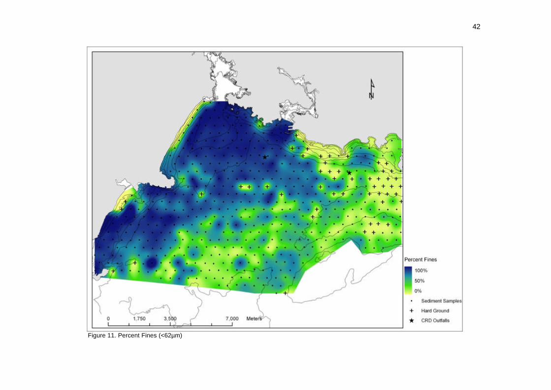
6.1.2 Fine Sediments The association between metals and fine sediments, particularly the fraction less than

62µm, is well documented (Zhang et al., 2001; Padmalal et al., 1996; Power and

Chapman, 1992; McLaren and Little, 1987; Young et al., 1985). In an effort to gain a

better understanding of the receiving environment, in terms of identifying areas of

potential contamination, the sediment data were mapped based on the percentage of

fines (<62µm) in each of the sediment samples (Figure 11). There are two areas within

Victoria Bight where sediment distributions have a high percentage of fine particles.

The northern portion of the study area, west of the entrance to Victoria Harbour, and the

southwestern section between Albert Head and William Head have the highest

percentage of fine particles. Along with other smaller pockets of fine sediments, the

areas described above likely have the greatest potential for elevated metal levels .

6.2 Derivation of Contaminant Values

6.2.1 Interpretation of FAA Light Absorbance Values Contaminant values for the metals of interest were determined using the light

absorbance values from the FAA instrument (Table A-3, Appendix 2). Light absorbance

values for calibration standards were plotted in an XY scatter plot and a line of best fit

was generated. The values from the equation of the line, y=mx + b, were incorporated

into the following expression:

×

−

=g

vm

by

x

)(

where x is the analyte concentration in µg g-1

y is the FAA light absorbance value

b is the y-intercept

m is the slope of the line

v is the volume to which the digestate was diluted to in mL

g is the amount of sediment analyzed in g

Resultant contaminant values (dry weight) are found in Table A-4, Appendix 2.

42

Figure 11. Percent Fines (<62µm)

43

6.2.2 Quality Assurance and Quality Control (QA/QC) QA/QC was carried out using method blanks and duplicate samples. The method

blanks were used to determine if any contaminants were being introduced during the

digestion procedure. The results of the method blank analysis are found in Table 4.

Table 4. Method Blank Values

Cr µg L-1 Cu µg L-1 Ni µg L-1 Zn µg L-1 BLANK 1 38.58 BDL 2.27 30.68

BLANK 2 27.52 26.3 18.82 36.88 BLANK 3 38.64 22.5 BDL 24.88 BLANK 4 BDL 22.5 BDL BDL BLANK 5 BDL 23.0 29.70 23.33 BLANK 6 BDL 17.4 BDL 25.55 Blank Avg 17.46 18.63 8.47 23.55

The values for the series of blanks were averaged, and the averaged values were

subtracted from each sample to obtain a corrected metal concentration (Table A-5,

Appendix 2). Samples below detection limit (BDL) were assigned a value of one half of

the detection limit (Pascoe, T. Pers. Comm., 2003). The detection limit for the FAA

instrument is taken as 1.0µg/g; therefore all BDL values were calculated as 0.50µg/g.

Duplicate samples were used to monitor the performance of the FAA instrument. For

each duplicate, the relative percent difference (RPD) was calculated:

+

−=

221()21(

100xxxx

RPD

where x1 and x2 are the concentrations of the analytes. The RPD values for the

duplicate samples are listed in Table 5. RPD values were evaluated based on the

following guidelines: An RPD between 0 -30 is considered good; 30-50 is fair; and 50+

is poor (Dodd, M. Pers. Comm., 2003). The average RPD value for Cr, Cu and Zn is

fair, indicating reliable results. Nickel had very poor RPD values and so the Ni data

were not used in the evaluation of metal contamination of the sediments in Victoria

Bight.

44

Table 5. Duplicate Samples: Measure of Relative Percent Difference (RPD)

ID Cr µg g-1 Cr µg g-1

dup Cr µg g-1

RPD Cu µg g-1 Cu µg g-1

dup Cu µg g-1

RPD Ni µg g -1 Ni µg g-1

dup Ni µg g-1

RPD Zn µg g-1 Zn µg g-1

dup Zn µg g-1

RPD

80 44.86 44.86 0.00 0.50 0.50 0.00 2.90 16.53 140.34 80.74 86.88 7.32 107 35.96 32.99 8.61 0.50 0.50 0.00 2.90 11.99 122.13 65.41 28.60 78.32 137 0.50 0.50 0.00 8.06 10.38 25.18 0.50 0.50 0.00 11.27 8.33 29.98 203 0.50 0.50 0.00 9.02 9.02 0.00 14.64 27.84 62.16 12.56 11.17 11.71 205 0.50 0.50 0.00 0.50 0.50 0.00 14.35 1.16 170.10 7.31 8.49 14.95 234 10.07 10.07 0.00 19.13 19.13 0.00 21.10 15.73 29.19 24.39 28.41 15.24 238 25.73 12.09 72.12 11.37 6.37 56.35 0.50 3.21 146.06 14.48 41.36 96.27 266 1.75 55.94 187.87 3.11 12.27 119.04 31.86 58.74 59.34 21.37 228.54 165.80 268 0.50 0.50 0.00 6.72 6.72 0.00 27.84 11.34 84.25 58.67 102.00 53.94 275 1.51 32.28 182.09 0.50 0.50 0.00 21.24 1.33 176.45 8.12 8.67 6.62 301 21.93 30.68 33.27 52.41 57.88 9.91 0.50 0.50 0.00 23.97 31.06 25.78 341 44.86 53.76 18.05 36.32 25.33 35.65 25.63 25.63 0.00 37.44 152.63 121.20 368 40.92 46.00 11.68 3.35 91.26 185.83 20.69 6.11 108.78 16.55 24.47 38.59 425 21.93 24.12 9.50 36.32 69.29 62.44 1.07 11.65 166.37 40.06 32.21 21.73 453 10.99 32.87 99.77 68.81 57.88 17.25 1.72 51.88 187.20 40.51 40.51 0.00 474 1.30 19.49 175.05 47.31 25.09 61.38 0.50 0.50 0.00 50.53 26.33 62.97 477 13.23 13.23 0.00 30.55 36.02 16.42 28.33 28.33 0.00 33.42 33.42 0.00 500 50.92 29.55 53.10 8.06 5.74 33.65 0.65 4.36 148.25 26.26 13.92 61.44 506 14.56 13.18 9.99 58.30 25.33 78.84 0.78 5.90 153.47 97.65 19.12 134.51 535 31.28 42.11 29.51 34.22 34.22 0.00 58.63 6.69 159.06 57.74 144.07 85.55 547 56.15 71.38 23.88 52.41 52.41 0.00 20.69 11.94 53.61 45.24 40.51 11.03 554 11.00 59.78 137.84 17.96 9.83 58.52 58.84 24.23 83.34 0.50 0.50 0.00

Average RPD 47.8 34.57 93.19 47.41

45

6.2.3 Potential Sources of Error In addition to the possible sources of error inherent in any field sampling program, and

the potential for sample contamination during laboratory analysis, the following possible

sources of error were identified during sample processing and analysis. During the

digestion procedure, the H2O2 used for the final 17 samples had surpassed the

indicated expiration date. The amount of effervescence generated from this H2O2 was

notably less than in previous instances. The samples affected were: 245, 205, 205D,

241, 207, 247, 278, 173, 104, 237, 168, 213, 50, 300, 180, 145, 582.

Problems with the FAA Ni lamp were noted during analysis. The lamp did not seat

properly into the lamp carriage. The light intensity from the Ni lamp was not satisfactory

when instrument parameters were set for Ni analysis. Alteration of parameter settings

resulted in acceptable light intensity. Light absorbance values for Ni were highly erratic

and the instrument had a great deal of difficulty obtaining a stable reading. As noted in

section 6.2.2 Ni data were not used to evaluate metal contamination in the study area.

6.3 Spatial and Statistical Analysis

6.3.1 Spatial Distribution of Metals Spatial analysis of the contaminant data was performed using ArcMap GIS software.

Surfaces for each of the metals tested were generated using a spline – tension

algorithm. Algorithm parameters were set to ensure that individual data points retained

their actual value. The maps created provide a visual representation of the distribution

and relative level of sediment contamination for Cr, Cu and Zn in Victoria Bight.

Chromium

The distribution of Cr in Victoria Bight is shown in Figure 12. Chromium distribution

appears to be somewhat erratic; however, at a broad scale Cr levels tend to be higher

in the northern section of the study area down to a latitude just south of Albert Head.

The higher levels of Cr in the northern section of the study area appear to coincide well

46

with the distribution of fine particles. In contrast, there are a number of areas where the

relationship between particle size and Cr levels is less distinct.

There are two groups of samples along the southern boundary of the study area where

Cr levels are elevated, and sediments have a relatively low percentage of fine particles,

particularly the group at the southeastern portion of the study area. A possible

explanation is the relationship between Cr and heavy mineral content in the sand

fraction. Certain heavy minerals are capable of adsorbing Cr (Padmalal et al., 1997). It

is possible that the sands in Victoria Bight are rich in these particular heavy minerals.

Another notable observation is the relatively low level of Cr in Parry Bay where the

sediments are dominated by fine particles, yet there does not seem to be a positive

relationship with Cr. Possibly the rates of deposition for fine sediment is very slow, and

consequently, the majority of the sediment in Parry Bay was deposited prior to

industrialization in the area, and has remained relatively undisturbed. William Head and

Albert Head may be acting as protective barriers, sheltering the sediments in Parry Bay

from currents and tides. William Head may be deflecting the incoming tide, and Albert

Head may shelter Parry Bay during the ebb flow. During the slightly stronger ebb,

Albert Head may cause a gyre to form, resulting in the deposition of sediments on the

south side of the point. This may account for the relatively high levels of Cr found here.

Copper

Copper levels in the study area are mapped in Figure 13. Copper concentrations are

highest in the northern portion of the study area, and this corresponds well with the

distribution of fine sediments in this area. Similar to Cr, there are relatively low Cu

levels in Parry Bay, with isolated high values immediately south of Albert Head. Again,

this is possibly the result of shelter from currents and tides provided by the headlands

on the west side of the study area, as described above. Also analogous to Cr levels,

there is a small group of samples at the south end of the study area, adjacent to William

Head, with elevated Cu levels.

47

Figure 12. Chromium Distribution

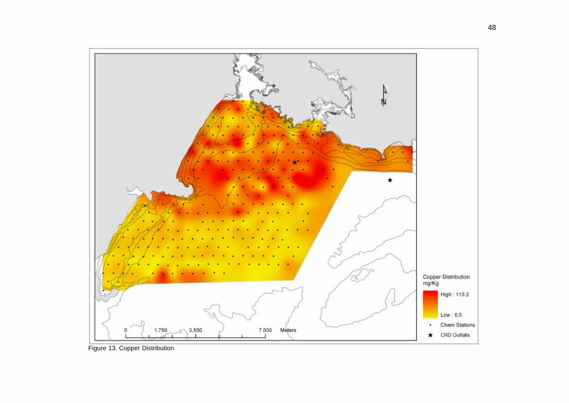
48

Figure 13. Copper Distribution

49

Zinc

While less pronounced than Cu, Zn levels in the northern portion of Victoria Bight are

generally higher than levels in the southern part of the study area (Figure 14). Again,

this corresponds well with fine particles. As was noted with both Cr and Cu, there are

relatively high Zn concentrations immediately south of Albert Head, and low Zn levels in

Parry Bay. Once more, this pattern may be explained by the hypothesis presented

regarding the Cr and Cu observations in this region. Unlike Cr and Cu, there is one

sample in Parry Bay, just north of William Head with a high Zn value. It is likely that this

sample is an anomaly, since the surrounding four samples all have similar low values.

A further similarity between Zn and the other metals are the elevated levels in the group

of samples at the south end of the study area adjacent to William Head. Being at the

edge of the study area, it is difficult to determine the cause for the elevated metal levels

in these samples, however, it seems to be a consistent zone of contaminant build-up.

50

Figure 14. Zinc Distribution

51

6.3.2 Statistical Analysis Statistical analysis was used to explore potential relationships between observed metal

values, and a number of other variables of interest. Statistics were also used to

supplement the insights gained from spatial analysis of sediment metal contamination in

Victoria Bight. While it is understood that statistics are not necessarily indicative of

cause and effect, nor does statistical significance necessarily translate into practical

significance, statistics are still useful in providing weight-of-evidence for hypotheses

testing (Sutherland, 2000; Luoma, 1990). All statistical analysis was performed using

the software package SPSS v. 10.0 for Windows . Data used for statistical analysis are

found in Table A-6, Appendix 2.

Raw metal values were used in descriptive and bivariate analysis. Multivariate analysis

was also performed, however prior to analysis the contaminant data were transformed

to generate two new data sets. The first data set was created using a log10+1

transformation. The log transformation serves to standardize the analyte values and

minimize the effects of differences in magnitude in data variability. The addition of the

constant 1 was used to avoid negative values (Emmerson et al., 1997; Brakstad, 1992).

The log data were further transformed by normalization to percent fines. This

transformation was employed to reduce the effects caused by variable grain-size (Birch

et al., 2001).

Descriptive Statistics

Basic descriptive statistics for Victoria Bight sediment samples are shown in Table 6.

In descriptive statistics the skewness value is a measure of data normality. In general,

a skewness value greater than 1.0 is an indication that data are significantly different

from a normal distribution. The skewness values in Table 6 indicate that Cr and Zn are

not normally distributed. Therefore, further analysis of the data was conducted using

non-parametric tests, which do not assume normally distributed data, or the log

transformed normalized data.

52

Table 6. Descriptive Statistics for Untransformed Data

N Range Minimum Maximum Mean Std. Dev. Variance Skew Std. Error % Fines 264 100 0.0 100.0 39.6 19.79 391.58 -0.22 0.15 % Moist 264 28.3 15.1 43.5 29.4 4.48 20.10 -0.24 0.15 Chromium 264 76.1 0.3 76.5 18.1 18.05 325.92 1.02 0.15 Copper 264 113 0.5 113.0 24.6 22.18 492.05 0.96 0.15 Zinc 264 285.6 0.5 286.1 37.5 44.06 1940.84 2.82 0.15 Valid N 264

Bivariate Analysis

Using Spearman’s Rank coefficient, the correlation between metal concentrations and a

number of variables of interest were examined. The first relationship explored was that

between metals and percent fines (Table 7). Copper and Zn are both significantly and

positively correlated to percent fines. That is, there is a linear relationship between Cu

and Zn levels and the percentage of fines in a sample. As the percentage of fine

particles increase, it is reasonable to assume that Cu and Zn levels could also

potentially increase. This supports the findings observed through spatial analysis.

According to the results in Table 7, Cr levels are not significantly related to particle size.

This may be a reflection of the association between Cr and coarser grained sediments

with heavy minerals capable of holding Cr.

Table 7. Correlations: Metals vs. % Fines

%

Fines Chromium Copper Zinc Spearman's rho % Fines Correlation Coefficient 1.000 -0.04 .262** .247** Sig. (2-tailed) . .520 .000 .000 N 264 264 264 264 ** Correlation is significant at the .01 level (2 tailed)

Another relationship examined was between metal levels and distance. In cases where

a single source of metal contamination dominates, with the exception of localized highs

in areas of secondary deposition, there is generally a decrease in contaminant levels

with increased distance from the source (Luoma, 1990). The values in Table 8 indicate

that there is a significant negative correlation between contaminant levels for all three

metals tested and distance from the Macaulay Point outfall. Therefore, in general, as

53

distance from the outfall increases, metal levels decrease. The relationship is strongest

for Cu and weakest for Cr. Distance was calculated from the Macaulay Point outfall

since very few of the samples are likely influenced by the Clover Point outfall based on

the dominant bottom currents.

Table 8. Correlations: Metals vs. Distance Distance Chromium Copper Zinc Spearman's rho Distance Correlation Coefficient 1.000 -.208** -.493** -.301** Sig. (2-tailed) . .001 .000 .000 N 264 264 264 264 ** Correlation is significant at the .01 level (2 tailed)

It should be noted that the Macaulay Point outfall is located in an area dominated by

fine sediments, with coarser sediments increasing with distance from the outfall. It is

likely that this has an influence on the correlation results given the demonstrated

association between metals and sediment grain-size. This would also account for the

relatively weak correlation between Cr and distance, based on the potential for Cr to

associate with coarser sediment fractions. Figure 15 illustrates the relationship between

each metal and distance from the outfall. The graphs, for Cr, Zn and to a lesser extent

Cu, indicate the possibility of secondary contamination, due to transport processes, at

varying distances from the outfall where metal levels increase with distance. This

supports some of the observations made through spatial analysis.

The final bivariate relationship investigated was between metal levels and direction from

the Macaulay Point outfall (Figure 16). Data from the 5 samples in the immediate

vicinity of Clover Point were not included in the analysis. The graphs indicate the mean

metal level for all samples in each of the 8 directions.

54

The results in Figure 16 should be interpreted with caution. As indicated by the values

in Table 9, the distribution of samples by direction is very uneven, with the vast majority

of samples being southwest of the outfall. Also, fine sediments are not evenly

distributed throughout the study area. Therefore, this will also affect the results since

most of the samples north-west of the outfall are fine sediments, and many samples

south and south-west of the outfall are coarser sediments.

55

Bearing in mind the limitations associated with the results presented in Figure 16, there

are some findings worth noting. For both Cr and Cu, mean levels are lowest in the

south and southwest directions. This coincides with bottom current data presented in

Figure 7a. Chromium results indicate highest mean values in the southeastern

direction, which also coincides with bottom current data, however, this result is based

on only 3 observations. Copper values also generally correspond to bottom current

data, with relatively high values in the east, southeast and western directions. Zinc

56

values also show similarities to bottom current data, exhibiting high levels in the eastern

direction. Zinc values for the north, south and southwest directions are relatively

similar, and this is also the case for current data. A notable departure from bottom

current patterns is the high Zn levels in the northeastern direction. Although less

obvious, this is also seen in Cu and Cr levels. The few samples northeast of the

Macaulay Point outfall are near the entrance to Victoria Harbour. This portion of the

study area overlaps with a sediment transport investigation conducted by GeoSea

Consulting. According to findings in the GeoSea report, there is sediment transport

occurring in the northeastern direction (from the Macaulay outfall) near the entrance of

Victoria Harbour (GeoSea, 1999). This may explain the discrepancy between observed

metal levels and bottom current data.

Multivariate Analysis

Principal components analysis (PCA) is a data reduction technique used to identify

principal components (PCs), or underlying factors, that are likely to explain the

distribution of environmental variables (Facchinelli et al., 2001; Brakstad, 1992). PCA

has been widely used to identify sources of metal contamination in sediments (Spencer,

2002; Birch et al., 2001; Simeonov et al., 2000; Salman and Abu Ruka’h, 1999; Ruiz et

al., 1998; Emmerson et al., 1997; Negrel, 1997; Huang et al., 1994; EVS, 1992b).

In an attempt to identify the likely source of metal contamination in Victoria Bight,

contaminant data were subject to PCA in two transformations. The first was a log

transformation, and the second was a log transformation normalized to percent fines.

PCA was conducted in three steps. The first was to examine if any correlation existed

between Cr, Cu and Zn. The data were then subject to tests to determine their

suitability for PCA. Finally, PCs were identified to explain variability in the data. The

components that accounted for the majority of the variability were extracted, and how

well each metal was explained by those components was indicated.

57

PCA: Log Transformed Data

Analysis indicates that all three metals tested are significantly, positively related to each

other (Table 10). This correlation between metals is often an indication that they come

from the same source (Luoma, 1990).

Table 10. Correlation Between Log Transformed Metals Log Cr Log Cu Log Zn Correlation Log Cr 1.000 .157 .147 Log Cu .157 1.000 .206 Log Zn .147 .206 1.000 Sig. (1-tailed) Log Cr .005 .008 Log Cu .005 .000 Log Zn .008 .000 Determinant = .921

The data suitability test results, for the log-transformed data, are displayed in Table 11.

The KMO value is greater than 0.50, therefore the PCA is likely to be useful in

explaining the data. The significance value related to the Bartlett’s test is less than

0.05, indicating that there is a significant relationship between the variables (metals).

Table 11. Data Suitability Test: Log Metals Kaiser-Meyer-Olkin Measure .572of Sampling Adequacy Bartlett's Test of Sphericity Approx. Chi-Square 21.468 df 3 Sig. .000

All of the variance in the data is explained by three PCs (Table 12). Of the three PCs

identified, the first PC, accounting for 44.7% of the variability in the data, was extracted.

The amount of variability for each metal explained by PC 1 is shown in Table 13. All

three metals loaded on the same PC. This indicates that it is reasonable to believe that

all three metals are from the same source. It should be noted however, that while

significant, the correlations in Table 10, the variance explained by PC 1, and the level of

variable loading on the extracted component are all fairly low. This is likely due to the

effects of variable grain-size (Birch et al., 2001).

58

Table 12. Total Variance Explained: Log Metals

Initial Eigenvalues Extraction Sums of Squared Loadings Component Total % of Variance Cumulative % Total % of Variance Cumulative %

1 1.341 44.693 44.693 1.341 44.693 44.6932 .865 28.841 73.534 3 .794 26.466 100.000

Extraction Method: Principal Component Analysis.

Table 13. Extracted Components: Log Metals

Component 1

Log Cr .617 Log Cu .698 Log Zn .687

Extraction Method: Principal Component Analysis. 1 component extracted.

PCA: Log Transformed Data Normalized to Percent Fines

Data normalized to percent fines were also subject to PCA. As noted by Birch et al.

(2001), removing the effects of gain-size is particularly useful when attempting to

identify sources of metal contamination in marine environments where there is a high

degree of variability in sediment characteristics. The correlation between the three

metals tested is far stronger having accounted for the effects of grain-size. The values

in Table 14 indicate that all three metals are almost perfectly positively correlated,

further supporting the hypothesis that all three contaminants originate at the same

source.

Table 14. Correlation Between Normalized Log Metals Cr Norm Cu Norm Zn Norm Correlation Cr Norm 1.000 .927 .850 Cu Norm .927 1.000 .849 Zn Norm .850 .849 1.000 Sig. (1-tailed) Cr Norm .000 .000 Cu Norm .000 .000 Zn Norm .000 .000 Determinant = 3.523E-02

Again, the data suitability tests indicate that PCA will be useful in explaining the

variability in the data, and that the variables are related to each other (Table 15). As

59

with the correlation results, the KMO value for the normalized data is higher than that for

the non-normalized data, indicating a relative increase in the ‘usefulness’ of the results.

Table 15. Data Suitability Test: Normalized Log Metals Kaiser-Meyer-Olkin Measure .757 of Sampling Adequacy

Bartlett's Test of Sphericity Approx. Chi-Square 867.145

df 3 Sig. .000

PCA of the data resulted in the identification of three PCs (Table 16). The first PC,

which accounts for 91.7% of the variability in the data, was extracted. Variable loadings

on the extracted PC were far stronger than those for non-normalized data, accounting

for almost 100% of the variability in each of the metals (Table 17). This is a strong

indication that the Cr, Cu and Zn found in the sediments of Victoria Bight are originating

at the same source.

Table 16. Total Variance Explained: Normalized Log Metals Initial Eigenvalues Extraction Sums of Squared Loadings Component Total % of Variance Cumulative % Total % of Variance Cumulative %

1 2.751 91.711 91.711 2.751 91.711 91.711 2 .176 5.862 97.573 3 7.281E -02 2.427 100.000

Extraction Method: Principal Component Analysis.

Table 17. Extracted Components: Normalized Log Metals Component 1

Norm Cr .967 Norm Cu .967 Norm Zn .938

Extraction Method: Principal Component Analysis. 1 component extracted.

Based on the observations and findings of spatial and statistical analyses, it is likely that

the primary source of metal contamination in Victoria Bight is the Macaulay Point outfall.

60

6.4 Sediment Contamination and Sustainable Development

6.4.1 Sustainable Development While there are numerous definitions of sustainable development (SD), in its simplest

form (simplest in terms of definition, certainly not in terms of implementation) it is

essentially a reconciliation of economic, social and ecological imperatives (Dale and

Hill, 1996). While the enormity of how to achieve sustainable development is well

beyond the scope of this research, there are a number of key components, or

underlying principles, of SD that are relevant to sewage related sediment contamination.

Biodiversity

The health and well-being of humans are linked and ultimately dependent on ecological

health. The loss of biodiversity at the species and ecosystem levels is one of the

greatest threats to society (Dale, 2001).

The ecosystem is comprised of four main components; air, water, land and biota.

Through a number of pathways each of these components are interconnected. The

contamination of any of these components may lead to the contamination of another

component. Sediments are a key element of the marine ecosystem. Because of their

physio-chemical properties, sediments are a sink for contaminants, and subsequently a

source of contamination for the ecosystem components to which they are linked.

Significant contamination of sediments may lead to species loss (Burton, 2002; Luoma,

1990).

The potential impacts of sediment related contamination is wide ranging. Deleterious

effects have been observed throughout the biota continuum; from benthic communities,

via direct exposure, to upper trophic levels (aquatic and terrestrial), through food-web

contamination (Burton, 2002). In marine environments, a key indicator of a severely

polluted or stressed environment is when biomass becomes greater than biodiversity.

This is caused by a replacement of many specialist species with a few tolerant

opportunistic species. This transformation is generally characterized by a reduction in

echinoderms and arthropods and an increase in polychaetes and molluscs (Anderlini

61

and Wear, 1992; Langston, 1990). Studies by EVS Consultants indicate that the

situation described above has been observed near the outfalls (EVS, 1992a,b). In

addition, during the sampling portion of this research, polychaetes -- specifically

annelids, were frequently recovered with sediment grab samples, and in a number of

cases near the Clover Point outfall, no sediment could be recovered because of thick

mussel beds.

The EVS reports describe the flourishing mussel and worm communities around the

outfalls as healthy, and indicative of low toxicity (EVS, 1992a,b). While the report

concedes that biomass is greater than biodiversity, around the outfalls, it does not

discuss the potential implications of this finding. The report also fails to address the

possibility that fauna found near the outfalls may have developed coping mechanisms

allowing them to thrive in toxic environments. Research on mussels has found that

exposure to metals can lead to the production of metallothionein (MT), and other metal-

binding proteins, allowing such organisms to tolerate metal induced toxicity. Therefore,

rather than using mussel communities as an indication of low toxicity, the measure of

MT production has been identified as a useful measure of contaminant related stress

(Langston, 1990).

Species that are intolerant to metal contamination can be adversely affected in a

number of ways. Impacts on reproduction and growth can impair the survival of

individuals, and affect populations and communities. Research has found that Cu can

be acutely toxic to microalgae at levels between 0.19µg l-1 and 0.30µg l-1and that Zn can

reduce growth at 15µg l-1 to 20µg l-1. Studies have also demonstrated impaired growth

of dinoflagellate assemblages resulting from Cu levels of 15µg l-1. Furthermore,

research has shown that recruitment can also be affected by metal contamination. This

phenomenon has been observed in clams (Macoma bathilica), which have

demonstrated an avoidance of contaminated sites (Langston, 1990).

Negative impacts related to metal contamination do not necessarily result from direct

toxicity. For example, contaminant -related changes to phytoplankton communities may

have serious consequences for higher trophic levels. A change in the phytoplankton

62

community structure can lead to a reduction in preferred prey species, and ultimately

the loss of higher trophic species in those communities. It is possible that the indirect

effects triggered by the loss of sensitive species have a much more significant impact

on marine communities than indicated by toxicity tests with an individual species

(Langston, 1990).

Scientific Uncertainty & the Precautionary Principle

One of the underlying philosophies of SD is the precautionary principle. Under this

paradigm, it is not acceptable to use scientific uncertainty as justification to postpone

action. The phrase ‘better safe than sorry’ is a good representation of the ideals behind

the precautionary principle. Under the current framework decision-makers require

scientific certainty, and more specifically proof of harm to justify actions to alter or

eliminate a potentially harmful activity. This certainly applies to the issue of sewage

disposal in Victoria. Ecological systems are immensely complex, and while science has

made great progress in understanding natural systems, there is still far more that is

unknown, than is known.

Toxic metals are continuously released into the environment, many of them

contaminating sediments. While some of the effects resulting from sediment

contamination have been documented, the true extent of short and long -term risks to

biota and humans is largely unresolved (Burton, 2002; Luoma, 1990). Most of the

toxicity studies have not addressed the implications of in situ short and long -term

exposures representative of the real world. Rather, the data only represent acute short-

term effects (Burton, 2002).

Much of the toxicity research conducted is performed on surrogate species. The

problem that results from studies on a particular species are not necessarily indicative

of the response of different species, even within the same genus. Furthermore, with

increased taxonomic difference comes increased probability that research findings will

not reflect true response (Chapman, 1991). Another inadequacy of toxicity research is

the frequent failure to account for compounding effects. For example, research on the

63

impacts of sewage discharge in the Fraser River Estuary revealed that although Hg, Cu

and Zn concentrations were not toxic to adult clams (Macoma bathilica), their combined

effect resulted in juvenile mortality and prevented settlement near the outfall (Langston,

1990). Toxicity testing data are the basis for many environmental guidelines, including

those developed for sediments. Unfortunately guidelines developed from these data do

not account for indirect effects such as bioaccumulation and transfer to higher trophic

levels (Burton, 2002). All of the metals studied in this research can potentially

bioaccumulate in certain marine organisms. Cu and Zn are essential to certain

biological functions, and organisms have developed mechanisms that regulate essential

metals. However, depending on environmental levels, regulatory mechanisms may be

incapable of coping with uptake levels leading to bioaccumulation (Rainbow, 1990).

6.4.2 Sediment Quality Guidelines All human activity has an impact on the environment. For a very long time, the

consequences of human activity were not recognized. Eventually, it became evident

that many anthropogenic activities were harmful to ecological systems. A mechanism

was necessary to link scientific findings to policies and regulations. Environmental

guidelines have been developed to monitor human impact on the environment, and to

gauge the quality of the environment. Over the last decade the importance of sediment

quality has gained a great deal of attention, and a number of sediment quality guidelines

(SQGs) have been developed in consequence.

Empirical data have been used to develop two general sets of SQGs based on

threshold levels. The first, ‘threshold level’ SQGs, define toxic levels below which

effects occur infrequently (LEL, TEL, ERL, MET, TEC); and the second, ‘effect level’

SQGs, define levels at which effects are expected to occur (AET, SEL, PEL, ERM, TET,

PEC). One of the earliest empirically-based SQGs were AETs developed by the WDOE

for sediments in Puget Sound. Unlike other ‘effect level’ SQGs, AETs are based on

significant effects always occurring and are therefore under-protective (Burton, 2002;

Birch et al., 2001). As noted in Section 2.2, the AETs developed by the WDOE are

64

currently used by the CRD to evaluate the sediments in Victoria Bight, despite their

inherent unsuitability (see Section 2.2).

The term ‘contamination’ is defined as the introduction of unwanted substances,

however; the term takes on an entirely new and subjective definition when used in

environmental assessment. For the purposes of environmental management, sediment

is only considered contaminated when it surpasses sediment quality guidelines (SQGs).

For this reason, understanding how the SQGs used were developed, and for what

purpose, is of critical importance when interpreting environmental data. The SQGs

used by the CRD are ‘effect level’ AETs. The guidelines for the three metals tested in

this research are shown in Table 18.

Table 18. CRD/WDOE Sediment Quality Guidelines Chromium µg g-1 Copper µg g-1 Zinc µg g-1

SQG 260.0 390.0 410.0 Results reported by EVS Consultants indicate that levels for Cr, Cu and Zn were all

highest at the Macaulay Point outfall sample station (Figure 2). None of the samples

surpassed the AET SQGs with maximum values for Cr, Cu and Zn reported as 59.4µg

g-1, 197.0µg g-1and 197.7µg g-1 respectively (EVS, 1992b). Therefore, based on the

SQGs in place, the CRD suggested that there is no evidence of metal contamination

from Cr, Cu or Zinc. To demonstrate the tremendous influence particular SQGs have

regarding policy and decision-making; the contaminant data from this research were

mapped based on various SQGs (Figures 17, 18, 19). As the figures indicate, the more

protective the SQG, the g reater the extent of contamination – in the regulatory sense.

By default, the more protective SQGs (LEL, TEL etc.) do a better job of accounting for

chronic sub-lethal effects, as opposed to AETs that are largely based on acute effects.

Ironically, proponents of the CRD’s LWMP argue that the discharge of untreated waste

is not a problem because of dilution and the self-cleansing properties of the receiving

environment. As noted by Langston (1990), this type of environment simply leads to a

much larger area subject to moderate levels of contamination, a situation where the

monitoring of chronic sub-lethal effects is far more appropriate to evaluate harm.

65

Figure 17. Chromium Sediment Quality Guidelines

66

Figure 18. Copper Sediment Quality Guidelines

67

Figure 19. Zinc Sediment Quality Guidelines

68

There are some implications to consider when using ‘effect level’ SQGs (SEL, PEL

etc.), particularly the under-protective AETs. Research indicates that ‘effect level’ SQG

values are s ignificantly above realistic environmental levels. This is particularly

applicable for the majority of coastal and off-shore marine environments; where dilution

can lead to a broad area of moderate contamination. The end result, when using ‘effect

level’ SQGs in coastal environments, is the appearance that impacts are restricted to

the immediate area of the contaminant source – while the potential for chronic damage

at the ecosystem level is unaccounted for (Langston, 1990). This precisely reflects the

current situation in Victoria Bight, where the CRD states that impacts are restricted to

the immediate vicinity of the outfalls (Taylor et al., 1998; EVS, 1992b).

Based on the discussion above, it is clear that the CRD’s current LWMP does not

conform to the principles of sustainable development. The loss of biodiversity and

subsequent damage at various trophic levels resulting from sewage contamination is a

significant possibility. Furthermore, there is a great deal of uncertainty, in regard to both

short and long-term chronic effects of sediment contamination, yet SQGs focused on

immediate acute effects are used. In order to become compliant with SD, the CRD’s

LWMP would have to undergo a number of changes: more protective SQGs would need

to be implemented, and the amount of contaminants discharged from the outfalls would

have to be minimized. There are two main methods for reducing sewage contaminant

loads: source control and treatment. The CRD suggests that its source control program

is sufficient, yet a report by the SLDF states that CRD documents indicate that there

has been no measurable reduction in contaminant load since the implementation of the

source control program (SLDF, 1999). Also, Cu has been established as one of the

worst marine contaminants and it is unlikely that source control alone will sufficiently

reduce Cu loadings since much of the current piping used in plumbing is Cu. Source

control alone also fails to address issues of non-compliance, and accidental releases.

To truly comply with SD, and minimize the amount of contaminants being discharged,

the CRD would have to incorporate both source control programs and waste treatment

facilities.

69

7.0 Conclusions

The research conducted for this study was carried out to accomplish the following:

• Determine the spatial distribution and level of metal contamination in surface

sediments in Victoria Bight, particularly Cr, Cu and Zn

• Determine if the sewage outfalls are the likely source of metal contamination

• Evaluate the current LWMP from a sustainable development perspective

Using GIS software to perform spatial analysis, the distribution of metal concentrations

in sediments in Victoria Bight was determined. Elevated metal levels were consistently

identified in three areas within the study area. The largest area is in the northern region

of the study area, near Royal Roads and extending southward to Albert Head. The

second zone of accumulation is immediately south of Albert Head, and the third area is

at the southern extent of the study area, immediately east of William Head. This may

indicate that contamination is occurring beyond Victoria Bight.

The physical characteristics of the receiving environment, along with observations made

during spatial analysis, were used in conjunction with statistical analyses to investigate

the source of elevated metal concentrations in the study area. Based on weight -of-

evidence, it is probable that the Macaulay Point outfall is the primary source of elevated

sediment metal levels in Victoria Bight.

The CRD’s current LWMP does not conform to the principles of sustainable

development. It is particularly lacking in the protection of biodiversity, and adherence to

the precautionary principle. Two major changes are necessary to rectify these

shortcomings. First, the CRD would have to use far more protective SQGs such as

LELs instead of AETs. Second, the CRD would have to implement an effective source

control program, and install waste treatment facilities, to minimize the amount of

contaminants being discharged into the receiving environment.

70

While this research has filled some of the knowledge gaps related to the sewage issue

in Victoria, it also serves to identify areas that require further research. Given the

relationship between contaminants, fine particles and depositional areas, a more

complete understanding of the dynamic behaviour of sediments in all of Victoria Bight

could prove very beneficial to environmental managers. In addition, this study is limited

in terms of chemical analyses. Analysis for a full suite of contaminants could potentially

provide a better understanding of the over all level of sediment contamination in Victoria

Bight. Finally, at a far broader level, this study has revealed that a great deal of

research is necessary to develop effective means of conveying the importance of

sustainable development to scientists and decision-makers alike.

71

References Anderlini, V.C., Wear, R.G. 1992. The effect of sewage and natural seasonal

disturbances on benthic macrofaunal communities in Fitzroy Bay, Wellington, New Zealand. Marine Pollution Bulletin, 24 (1): 21-26.

Birch, G.F., Taylor, S.E., Matthai, C. 2001. Small-scale spatial and temporal variance in

the concentration of heavy metals in aquatic sediments: a review and some new concepts. Environmental Pollution, 113 : 357-372.

Birch, G.F. 1996. Sediment-bound metallic contaminants in Sydney’s estuaries and

adjacent offshore, Australia. Estuarine, Coastal and Shelf Science, 42: 31-44. Brakstad, F. 1992. A comprehensive pollution survey of polychlorinated dibenzo-p-

dioxins and dibenzofurans by means of principal component analysis and partial least squares regression. Chemosphere, 25 (11): 1611-1629.

Burton Jr., G.A. 2002. Sediment quality criteria in use around the world. Limnology, 3:

65-75. Chague-Goff, C., Rosen, M.R. 2001. Using sediment chemistry to determine the impact

of treated wastewater discharge on a natural wetland in New Zealand. Environmental Geology, 40 : 1411-1423.

Chapman, P.M. 1991. Environmental quality criteria: what type should we be

developing? Environmental Science & Technology, 25 (8): 1353-1359. Cleverly, B. 2001. CRD director urges colleagues to halt dumping of raw sewage in

Victoria. Victoria Times Colonist. February 8, 2001. Victoria, B.C. Connelly, J. 1999. Canada’s sewage system a ‘disgrace’. Report gives Victoria ‘F’ for

fouling strait. Seattle Post-Intelligencer. Seattle, WA. CRD. 2000. Capital regional district core area liquid waste management plan. Capital

Regional District, Victoria, B.C. Crone, T.J., Ebbesmeyer, C.C., Ingraham Jr., W.J. 1998. Dispersion of 1,000 drift

cards released over Victoria’s sewage outfalls. Puget Sound Research ’98. Obtained from: http://www.wa.gov/puget_sound/Publications/98_proceedings/pdfs/2a_crone.pdf

Dale, A. 2001. At the edge: sustainable development in the 21st century. UBC Press,

Vancouver, B.C. 212 pp.

72

Dale, A., Hill, S.B. 1996. Biodiversity conservation: A decision-making context. In Achieving sustainable development. Edited by A. Dale & J.B. Robinson. UBC Press, Vancouver, B.C. 303 pp.

Emmerson, R.H.C., O’Reilly-Wiese, S.B., Macleod, C.L., Lester, J.N. 1997. A

multivariate assessment of metal distribution in inter-tidal sediments of the Blackwater Estuary, UK. Marine Pollution Bulletin, 34 (11): 960-967.

EVS Consultants and Virginia Institute of Marine Science. 1992a. Sediment profile

imaging (SPI) survey of the seafloor off Macaulay and Clover Point wastewater outfalls Victoria, B.C. EVS Project No. 3/073-10. Vancouver, B.C.

EVS Consultants. 1992b. Sediment and related investigations off the Macaulay and

Clover Point sewage outfalls. EVS Project No. 3/073-11. Vancouver, B.C. Facchinelli, A., Sacchi, E., Mallen, L. 2001. Multivariate statistical and GIS-based

approach to identify heavy metal sources in soils. Environmental Pollution 114: 313-324.

GeoSea Consulting. 1999. A sediment trend analysis (STA®) of Victoria Harbour.

Victoria, B.C. Unpublished report. GeoSea Consulting. 2000. GeoSea Laboratory Manual. Victoria, B.C. Internal

technical document. Ginn, T.C., Pastorok, R.A. 1992. Assessment and management of contaminated

sediments in Puget Sound. In Sediment toxicity assessment. Edited by G.A. Burton Jr. Lewis Publishers. Boca Raton, FL. 457 pp.

Hewitt, A.T., Mosher, D.C. 2001. Late Quaternary stratigraphy and seafloor geology of

eastern Juan de Fuca strait, British Columbia and Washington. Marine Geology, 177: 295-316.

Huang, W., Campredon, R., Abrao, J.J., Bernat, M., Latouche, C. 1994. Variation of

heavy metals in recent sediments from Piratininga Lagoon (Brazil): interpretation of geochemical data with the aid of multivariate analysis. Environmental Geology, 23: 241-247.

Langston, W. J., 1990. Toxic effects of metals and the incidence of metal pollution in

marine ecosystems. In Heavy metals in the marine environment. Edited by R.W. Furness and P.S. Rainbow. CRC Press. Boca Raton, FL. 256 pp.

Luoma, S.N. 1990. Processes affecting metal concentrations in estuarine and coastal

marine sediments. In Heavy metals in the marine environment. Edited by R.W. Furness and P.S. Rainbow. CRC Press. Boca Raton, FL. 256 pp.

73

McLaren, P., Little, D.I. 1987. The effects of sediment transport on contaminant dispersal: An example from Milford Haven. Marine Pollution Bulletin, 18 (11): 586-594.

Negrel, P. 1997. Multi-element chemistry of Loire Estuary sediments: Anthropogenic

vs. natural sources. Estuarine, Coastal and Shelf Science, 44: 395-410. Padmalal, D., Maya, K., Seralathan, P. 1997. Geochemistry of Cu, Co, Ni, Zn, Cd and

Cr in the surficial sediments of a tropical estuary, southwest coast of India: a granulometric approach. Environmental Geology, 31: 85-93.

Paetzel, M., Nes, G., Leifsen, L.O., Schrader, H. 2002. Sediment pollution in the

Vagen, Bergen harbour, Norway. Environmental Geology, Springer-Verlag, online. Palmer, M.D. 1999. Analyses of sediment bacteria monitoring data from two deep

ocean raw wastewater outfalls, Victoria, BC. Canadian Water Resources Journal 25 (1): 1-18.

Power, A.E., Chapman, P.M. 1992. Assessing sediment quality. In Sediment toxicity

assessment. Edited by G.A. Burton Jr. Lewis Publishers. Boca Raton, FL. 457 pp.

Rainbow, P.S. 1990. Heavy metal levels in marine invertebrates. In Heavy metals in

the marine environment. Edited by R.W. Furness and P.S. Rainbow. CRC Press. Boca Raton, FL. 256 pp.

Rainbow, P.S., Furness, R.W. 1990. Heavy metals in the marine environment. In

Heavy metals in the marine environment. Edited by R.W. Furness and P.S. Rainbow. CRC Press. Boca Raton, FL. 256 pp.

Rogers, V.J. 1995. Wastewater treatment utilizing wastewater outfalls: The role of

science, communications and public involvement in the decision-making process. Water Science and Technology, 32 (2): 1-8.

Ruiz, F., Gonzalez-Regalado, M.L., Borrego, J., Morales, J.A., Pendon, J.G., Munoz,

J.M. 1998. Stratigraphic sequence, elemental concentrations and heavy metal pollution in Holocene sediments from the Tinto-Odiel Estuary, southwestern Spain. Environmental Geology, 34 (4): 270-278.

Salman, S.R., Abu Ruka’h, Y.H. 1999. Multivariate and principal component statistical

analysis of contamination in urban and agricultural soils from north Jordan. Environmental Geology, 38 (3): 265-270.

Sanudo-Wilhelmy, S.A., Olsen, K.A., Scelfo, J.M., Foster, T.D., Flegal, A.R. 2002.

Trace metal distributions off the Antarctic Peninsula in the Weddell Sea. Marine Chemistry, 77: 157-170.

74

Simeonov, V., Massart, D.L., Andreev, S., Tsakovski, S. 2000. Assessment of metal

pollution based on multivariate statistical modeling of ‘hot spot’ sediments from the Black Sea. Chemosphere, 41: 1411-1417.

SLDF. 1999. The national sewage report card (number two). A Sierra Legal Defence

Fund Report. Obtained from: http://www.sierralegal.org/reports_1999.html Spencer, K.L. 2002. Spatial variability of metals in the inter-tidal sediments of the

Medway Estuary, Kent, UK. Marine Pollution Bulletin, 44 : 933-944. Sutherland, R.A. 2000. A comparison of geochemical information obtained from two

fluvial bed sediment fractions. Environmental Geology, 39 (3-4): 330-342. Taylor, L.A., Chapman, P.M., Miller, R.A., Pym, R.V. 1998. The effects of untreated

municipal sewage discharge to the marine environment off Victoria, British Columbia, Canada. Water Science and Technology, 38 (10): 285-292.

Thomson, R.E. 1981. Oceanography of the British Columbia Coast. Canada Special

Publications. Fisheries and Aquatic Sciences. Canada. 56: 291 pp. Turner, A., Millward, G.E. 1994. Partitioning of trace metals in a macrotidal estuary.

Implications for contaminant transport models. Estuarine, Coastal and Shelf Science, 39: 45-58.

U.S. EPA. 1986. Test methods for evaluating solid wastes. U.S. Environmental

Protection Agency, Office of Solid Waste and Energy Response, Washington, D.C. Obtained from: http://www.epa.gov/epaoswer/hazwaste/test/main.htm

Werring, J. 1999. Fishing union takes Capital Regional District to court for dumping raw

sewage into Juan de Fuca Strait. Sierra Legal Defence Fund Press Release. Obtained from: http://www.sierralegal.org/m_archive/pr99_02_04.htm

Werring, J., Chapman, D. 1999. Synopsis. Excerpt from a prosecution brief.

Unpublished. Young, R.A., Swift, D.J.P., Clarke, T.L., Harvey, G.R., Betzer, P.R. 1985. Dispersal

pathways for particle-associated pollutants. Science, 229 (4712): 431-435. Zhang, W., Yu, L., Hutchinson, S.M., Xu, S., Chen, Z., Gao, X. 2001. China’s Yangtze

Estuary: I. geomorphic influence on heavy metal accumulation in intertidal sediments. Geomorphology, 41: 195-205.