CjioftS

CYCLIC LTI SYSTEMS IN DIGITAL SIGNAL PROCESSING

P. P. Vaidyanathan, Fellow, IEEE and A. Kirac, student member, IEEE

Dept. of Electrical Engineering, Caltech, Pasadena, CA 91125, USA

Ph:(626) 395 4681 email:ppvnath@sys.caltech.edu

EDICS CATEGORY: 2.4.2

Abstract Cyclic signal processing refers to situations where all the time indices are interpreted modulo some

integer L. In such cases the frequency domain is defined as a uniform discrete grid (as in i-point DFT).

This offers more freedom in theoretical as well as design aspects. While circular convolution has been the

centerpiece of many algorithms in signal processing for decades, such freedom, especially from the viewpoint

of linear system theory, has not been studied in the past. In this paper we introduce the fundamentals

of cyclic multirate systems and filter banks, presenting several important differences between the cyclic

and noncyclic cases. Cyclic systems with allpass and paraunitary properties are studied. The paraunitary

interpolation problem is introduced and it is shown that the interpolation does not always succeed. State

space descriptions of cyclic LTI systems are introduced, and the notions of reachability and observability

of state equations revisited. It is shown that unlike in traditional linear systems, these two notions are not

related to the system minimality in a simple way Throughout the paper, a number of open problems are

pointed out from the perspective of the signal processor as well as the system theorist.

1. INTRODUCTION

Consider two sequences x(n) and h(n) defined for 0 < n < L - 1, and let y{n) denote their circular or cyclic

convolution [17]. That is, y(n) = £m=ox(m)Mn ~ m) with a11 arguments interpreted modulo L. We can

represent this operation by the block diagram of Fig. 1 where x(n) and y(n) are the input and output,

respectively, of a linear system. With all time-arguments interpreted modulo-!,, this is also a time-invariant

system (i.e., a circular-shift invariant system). We say that {h(n)} is a cyclic LTI system. For the purpose of

interpretation one can also regard x(n) to be a periodic-L input, for which the LTI system h(n) yields the

periodic-L output y(n).

Circular or cyclic convolution has been at the center of digital signal processing from its early days [8].

Indeed, fast algorithms for ordinary convolution routinely convert the problem into a cyclic convolution and

Work supported in parts by the Office of Naval Research Grant N00014-93-1-0231, and Tektronix, Inc.

DISTRIBUTION STATEMENT A

Approved for public release; Distribution Unlimited 19980707 126

>

then use the FFT. The notion of polynomial transforms introduced by Nussbaumer [16] is another example

of the prevalence of these ideas in the early days of digital signal processing. Most of the classical applica-

tions involving cyclic convolutions are based on the important result that cyclic convolution corresponds to

multiplication of the DFT coefficients, that is, Y(k) = H(k)X(k) for 0 < k < L - 1. Further properties of

cyclic LTI systems from the viewpoint of multirate signal processing (more generally linear system theory)

have not been studied in the past. In this paper we will consider a number of such properties. The emphasis

will be on well-known topics [1], [12], [23], [27] such as multirate systems, filter banks, paraunitary matrices,

and state space representations, but this time in a cyclic setting.

1.1. Motivation and Scope

The frequency response of a cyclic LTI system is the L-point DFT of the impulse response:

L-l

H(k) = Y,h(n)W£n, 0<k<L-l, (1) n=0

where WL = e-j2v/L. This is equivalent to sampling the conventional frequency response £n=o h(n)e-ju,n

at L discrete values of the frequency uk = e^k'L (the DFT-frequencies, Fig. 2). The basic building blocks

in the implementation of this system are multipliers, adders, and cyclic delays W£. The cyclic delay, indicated

in Fig. 3, has input-output relation y(n) = x(n - 1) where the time-arguments are interpreted modulo-L.

Fig. 4 shows the direct-form structure for H(k), using these building blocks.

In cyclic signal processing, the frequency domain is defined as a set of L discrete frequencies rather than

the entire range 0 < w < 2n. This offers more freedom in theoretical developments. For example, we will

see in Sec. 4 that the definitions of allpass filters and paraunitary matrices are less restricted in the cyclic

world. Similarly orthonormal filter banks in the cyclic world are less restrictive. In subband and transform

coding problems, if the power spectrum of the input signal is defined only over a discrete grid of frequencies

and the filters optimized for these frequencies, it might offer an increased coding efficiency. Likewise, in

filter design problems one traditionally imposes constraints (e.g., linearity of phase) and optimizes the filter

with respect to some criterion (e.g., minimax, minimum error energy, etc.). These constraints are now only

over a discrete grid rather than a continuous range of frequencies. These are some of the motivations for

considering cyclic signal processing as a theoretical discipline by itself. The practical advantages obtained

using this viewpoint can be significant, but it requires further detailed work to quantify these advantages

for specific applications. A unique example of the use of cyclic filter banks (brought to our attention by one

of the reviewers) is the method of autoregressive spectral estimation in subbands, advanced by Nishikawa et

al. in 1993 [14]. Our emphasis in this paper will only be on the theoretical differences between cyclic and

noncyclic systems, especially pertaining to multirate systems, filter banks, and LTI system theory.

2

0TIC QUALITY XX3FECT» 1

►

Related literature. Since circular convolution is an integral part of DSP, we can regard cyclic LTI filtering

as one of the earliest known DSP techniques [8]. The use of circular filtering in image subband coding (where

images have finite size [7]) was motivated by the work of Smith and Eddins on symmetric extension techniques

[19]. Circular convolution for subband coding was also explicitly considered by Kiya, et al [11]. In 1993,

Caire et al [5] introduced wavelet transforms associated with cyclic groups. Cyclic versions of two-channel

filter-bank orthonormality and power complementarity can already be found in that paper. More recently

cylic multirate system basics were explicitly formulated in two independent conference papers [24], [3]. While

both papers start with a common basic theme, the work by Bopardikar, et al [3], [4] eventually focuses on

the wavelet aspect whereas [24] focuses on system theoretic aspects, factorizations and so forth. The very

recent work in [13] focuses on interesting details of the two channel linear phase orthonormal case. In this

paper the emphasis will be more along the lines of [24-26].

1.2. Notations and Abbreviations

• WL = e~j2'r/'L, with the subscript deleted if obvious.

• The integer k is reserved for the frequency index in the DFT expressions. Throughout the paper, k is

therefore analogous to frequency.

• In the figures W£ denotes one unit of cyclic delay, that is, y(n) = x(n -1) with n -1 interpreted modulo

L. This is analogous to z~l or e~ju in standard DSP block diagrams.

• The abbreviation siso stands for single-input single-output, and mimo for multi-input multi-output.

• The abbreviation PU stands for paraunitary.

• Matrices and vectors are denoted by bold letters. The notations AT, A*, and AT denote, respectively,

the transpose, the conjugate, and the transpose-conjugate of A.

• The tilde notation is defined as follows: H(z) = H'(1/z*).

1.3. Outline

Sec. 2 introduces the basic building blocks for cyclic DSP. This includes filtering structures, cyclic difference

equations, decimators, expanders, polyphase representations of cyclic filter banks, Nyquist property, and so

forth. Sec. 3 considers cyclic versions of allpass and paraunitary properties, and introduces cyclic orthonor-

mal filter banks. Sec. 4 studies some basic differences between the cyclic and noncyclic cases. For example we

show that a cyclic-LTT system can be paraunitary or allpass, even though the noncyclic counterpart (defined

therein) may not have this property. This shows that such properties are less restrictive in the cyclic case. In

Sec. 5 we consider the paraunitary interpolation problem. We show again that noncyclic interpolants (more

general than noncyclic counterparts) do not in general share the property of the underlying cyclic system.

3

>

For example we will show that there are cyclic paraunitary matrices which do not have FIR paraunitary in-

terpolates, though IIR paraunitary interpolants always exist. In Sec. 6 we introduce state space descriptions

of cyclic LTI systems. We also revisit the traditional notions of reachability and observability in the context

of state space descriptions. We show that unlike in noncyclic systems these concepts do not have a simple

relation to the so-called minimality of the structure. Throughout the paper we will point out a number of

open problems pertaining to cyclic DSP systems.

2. BASICS OF CYCLIC DIGITAL FILTERS AND MULTIRATE SYSTEMS

2.1. Filtering Structures For Cyclic Digital Filters

Using the idea that W£ represents a cyclic(L) delay (analogous to z_1) we can draw structures for cyclic-

LTI systems as demonstrated in Fig. 4. In general this requires L multipliers. By expressing the frequency

response in rational form we can sometimes obtain more efficient implementations. Thus, consider the

example of a cyclic-L transfer function

H(k) - *o + aiW£ (2)

The direct-form structure for this is shown in Fig. 5, and the input and output of this system are constrained

by (1 - bW£)Y(k) = (a0 + ai W£)X(k). By taking the inverse DFT of this equation we obtain the recursive

difference equation (d.e.)

y(n) = by[n -1)4- a0x(ji) + aix(n - 1) (3)

Since the time-indices are interpreted modulo L, this is a cyclic difference equation. It is therefore tricky to

establish an initial condition for this equation. To demonstrate why this is the case, let L = 3. Repeated

use of the difference equation (and using the facts that y(2) = j/(-l), y(3) = y(0) and so forth) yields the

conclusion

(1 - b3)y(0) = a0x(0) + aix(l) + a2x(2)

for some constants a,. Thus the initial condition y(0) is not arbitrary. It is uniquely determined as long as

63 7^ 1, that is, as long as b ^ Wj for any i. This condition on b is equivalent to the obvious requirement

that the denominator in (2) does not become zero for any k. We can then write Y(k) = H(k)X(k), and the

inverse DFT y(n) is fully determined for all n. More generally, consider the cyclic(L) transfer function

()"i + 5£iW*2" With the implicit assumption that H(k) is defined for all k (i.e., the preceding denominator does not vanish

for any fc), the output is fully determined by the input. In particular the "initial" condition is predetermined,

4

>

rather than arbitrary. Fig. 6 shows the direct-form implementation of this system. As a generalization of

the difference equation idea, we will study in Sec. 6 state space descriptions of cyclic LTI systems.

Even though the "initial" condition has to be computed separately, the use of a recursive structure

often results in reduced computation. For example, consider the cyclic LTI system with frequency response

H(k) = En=o anW£n. This can be implemented as shown in Fig. 4, requiring L multipliers and L - 1

adders. However, we can find a more efficient recursive implementation by rewriting

H(k) -ga-Wf = I^ (5) n=0 L

The expression on the right hand side yields a recursive implementation which requires only two multipliers

and one adder.

2.2. Cyclic Decimators and Expanders

The cyclic decimator, denoted by | M in Fig. 7(a), has the input-output relation y(n) = x(Mn). We assume

throughout the paper that M is a factor of L, that isj

L = MK, K= integer (6)

With x(n) regarded as cyclic(L), the output y(n) is cyclic(üQ as demonstrated in Fig. 7(b), 7(c). Let X(k)

denote the L-point DFT of x(n) and Y(k) the K-point DFT of y(n), that is, X(k) = EÜ *(»)WE^ ° ^

k < L - 1 and Y(k) = J2n=o y(n)WK°> 0 <k < K-l.lt can. then be verified (Appendix A) that

M-l

Y(k) = -T7^X{k- iK) (cyclic decimator), (7) i=0

forO<k<K-l. Thus the DFT Y(k) is obtained by superposing M shifted copies of the DFT X(k) where

the shifts are in multiplies of K. This is the counterpart of the traditional aliasing formula for decimators

[23]. The cyclic expander, denoted by T M in Fig. 8(a), has a periodic-X input x(n) and periodic-L output

y(n) related by

ytn\ = { x{n/M), n = mul. of M ^ 10 otherwise.

This is demonstrated in Fig. 8(b), 8(c). The corresponding DFT relation is

Y{k) = X(k) (cyclic expander), (9)

t If this is not the case, then decimation by M would retain more samples than one-out-of M. For

example, if M and L have no common factors, then there is no loss of samples at all, and the decimated

output is a permuted version of the input samples.

5

for 0 < k < L - 1. (This is similar to the periodic extension idea in DFT theory [8]). Since X(k) are the

tf-point DFT coefficients of x(n), the L-point DFT Y{k) has the period K = L/M. We can define fractional

decimators in a manner analogous to the noncyclic case (for example, as in Fig. 4.1-10 of [23]). We leave it

to the reader to figure out the details.

2.3. Polyphase Representation

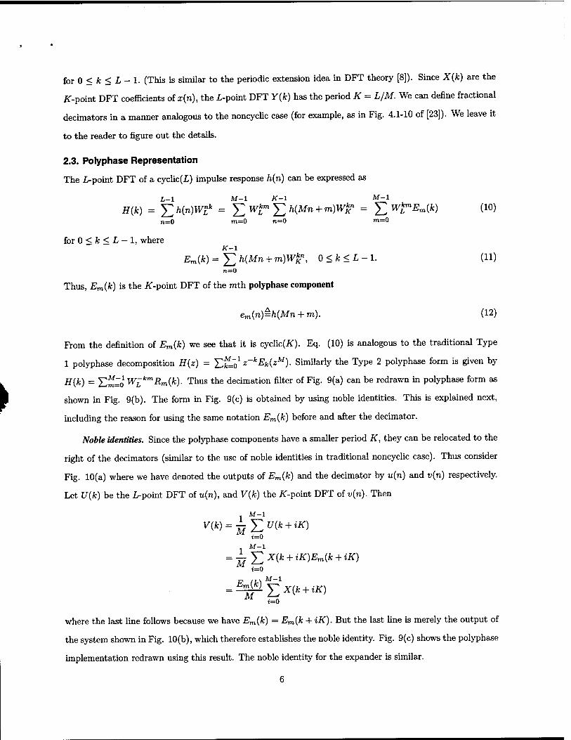
The L-point DFT of a cyclic(L) impulse response h(n) can be expressed as

L-l M-l K-l M-l

H(k) = J2h(n)W2k = £w£m5>(Mn + m)W£" = £ WkmEm{k) (10) n=0 m=0 n=0 m=0

for 0 < k < L — 1, where K-l

Em(k) = £ h(Mn + ro)W£n, 0 < k < L - 1. (11)

Thus, Em(k) is the i^-point DFT of the mth polyphase component

em(n)=h(Mn + m). (12)

From the definition of Em(k) we see that it is cyclic(Är). Eq. (10) is analogous to the traditional Type

1 polyphase decomposition H(z) = Efcl'o1 z~kEk(zM). Similarly the Type 2 polyphase form is given by

H{k) = Em=o W[kmRm(k). Thus the decimation filter of Fig. 9(a) can be redrawn in polyphase form as

shown in Fig. 9(b). The form in Fig. 9(c) is obtained by using noble identities. This is explained next,

including the reason for using the same notation Em(k) before and after the decimator.

Noble identities. Since the polyphase components have a smaller period K, they can be relocated to the

right of the decimators (similar to the use of noble identities in traditional noncyclic case). Thus consider

Fig. 10(a) where we have denoted the outputs of Em(k) and the decimator by u(n) and v{n) respectively.

Let U(k) be the L-point DFT of u(n), and V(k) the tf-point DFT of v(n). Then

1 M-l

t=0

1 M-l

= 77 51 X(fc + iK)Em(k + iK) i=0

„ ,,. M-l

i=0

where the last line follows because we have Em(k) = Em(k + iK). But the last line is merely the output of

the system shown in Fig. 10(b), which therefore establishes the noble identity. Fig. 9(c) shows the polyphase

implementation redrawn using this result. The noble identity for the expander is similar.

6

A caution regarding notation, however, is in order. We have used the same notation Em(k) for the

mth polyphase component in Figs. 9(b) and 9(c). This is regarded as a ÜT-point DFT in Fig. 9(c) and an

i-point DFT (with values repeating after a shorter period K) in Fig. 9(b). The (cyclic) impulse response

of the filter Em(k) is accordingly as shown in Fig. 10, before and after the decimator. If this distinction is

not clear from the context, one has to use a superscript as in Em (k) (before decimator) and Em '(k) (after

decimator).

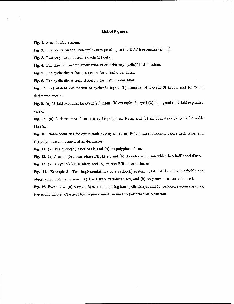
Now consider the analysis/synthesis system of Fig. 11(a). With the filters Hi{k) represented in Type

1 polyphase form and the filters Fi(k) in Type 2 form, we have the equivalent representation of Fig. 11(b)

where E(&) and R(fc) are the polyphase matrices of the cyclic filter bank. These should be interpreted as

Appoint DFTs, e.g.,

E(*)=£e(n)W£\ (13) n=0

The filter bank has the perfect reconstruction property x(n) = x(n) if and only if the equation R(/c)E(fc) = I

is satisfied for all the K values of k. With a slightly more general definition, one can obtain the analog of Eq.

(5.6.7) in [23]. The alias-component (AC) matrix, which is very useful in the noncyclic case [23], can also be

defined for the cyclic case, and the alias-free and perfect reconstruction conditions can be formulated using

this. See Appendix B which also shows the relation between the cyclic-AC matrix H(fc) and the polyphase

matrix E(fc), which can be used to express orthonormality directly in terms of the filters hi(n).

3. ALLPASS AND PARAUNITARY PROPERTIES

The allpass property and more generally the paraunitary property play a crucial role in digital filtering, and

in the theory and implementation of multirate filter banks. We now extend these ideas to the cyclic case.

3.1. Cyclic Allpass Filters

A cyclic(L) allpass system is one for which H{k) = eJ*(fc) forO<fc<L-l.A simple example is the first

order system b* + W$

We can always rewrite any cyclic allpass system H{k) — eJ'*(fc) in rational form

rS^J h* Wfcn

H{k) = C1-nf0j-nWuL , |c| = l. (15)

For example, we can let J = L - 1 and set e-^*)/2 = Y,nZl bnW£n. The coefficients bn are essentially the

inverse DFT coefficients of e~iWW2 and can readily be identified. More interesting is the open problem of

obtaining the rational form with smallest order J.

The allpass property in the cyclic case can be expressed entirely in terms of the unitary property of a

circulant matrix. For this consider the L x L circulant matrix H formed from the impulse response h(k),

demonstrated below for L = 4.

H =

fc(0) ft(l) /i(2) ft(3) fc(3) h{0) h(l) h(2) h{2) /i(3) h(0) h(l)

L/i(l) h(2) fc(3) fc(0)J

We know that circulant matrices are diagonalized by the DFT matrix (which is unitary) and that the

eigenvalues are the DFT coefficients H(k). That is,

__ WAWt

where wtw = MI and A is a diagonal matrix with elements H(k). Using this we can see that HTH = I if

and only if \H(k)\ = 1. Thus the cyclic allpass property is equivalent to the unitariness of the matrix H.

The rational form (15) has nonzero denominator for all k as long as the L-point DFT of {bn} is nonzero

for all k. Equivalently, the polynomial £n bnz~n should have no zeros at the unit-circle points z = W£. For

the allpass case we can assume further that £„ bnz~n has no zeros anywhere on the unit circle because such

a zero would also be present in Y?n=<s bJ-nz~n and can be cancelled anyway. Thus, any cyclic allpass system

can be written as in Eq. (15) where bn are such that X)„ bnz~n is free from unit circle zeros.

3.2. Cyclic Paraunitary Systems and Orthonormal Filter Banks

The M xM cyclic transfer matrix E(fc) is said to be cyclic-paraunitary (or cyclic-PU) if it is unitary for all

k. In Sec. 4 and 5 we consider the properties of cyclic-paraunitary systems in greater detail and show that

they do not share some of the restrictions of noncyclic PU systems.

We define the M-band cyclic filter bank (Fig. 11(a)) to be orthonormal if the polyphase matrix E(fc)

is unitary for all k. That is, E(fc) is cyclic-PU. The perfect reconstruction property then reduces to R(fc) =

Et(fc), which can be rewritten in terms of the cyclic(L) impulse responses as

fi(n) = h*(-n). (16)

The DFTs are correspondingly related as Fj(fc) = H*(k). Recall here that the arguments of hi(.), /,(.),

Hi(.) and Fi(.) are interpreted modulo L. The above definition of orthonormality is consistent with the

statement that the filter bank expands the cyclic(L) signal x(n) using an orthonormal basis. Thus, assuming

x(n) = x(n) in Fig. 11(a) we have

M-1K-1

*(") =EE uiW/i(n " iM)> 0 < n < L - 1. (17) i=0 1=0

The basis functions are the length-i sequences

rn,e(n)=fi(n-^M), 0<n<L-l (18)

where 0<*<M-l,0<£<uf-l. Thus there are MK = L basis functions r]Ui{ji). It can be shown that

the unitarity of R(fe) is equivalent to orthonormality of the basis »fc,«(n) (Appendix B). This orthonormality

can be reexpressed as

J2fi(n)&(n-Mt) = 6(i-m)6(£) (19) n=0

As in traditional filter banks, orthonormality of the cyclic filter bank implies:

1. Unit-energy property: Y^t=o l/t(n)l2 = 1 for a11 * (and similarly for hi(n)).

2. Power complementary property: E^Q1 |-Fi(*:)|2 = M, for all k (and similarly for Ht(k)).

4. CYCLIC VERSUS NONCYCLIC SYSTEMS

There are several basic differences between the behaviors of cyclic and noncyclic LTI systems. To demon-

strate, consider the determinant of a paraunitary matrix. For the noncyclic case, this can be shown to

be an allpass function [23]. If E(fc) is cyclic paraunitary, then the same result can be proved, that is,

[det E(fc)] = eJ'*(fc) = allpass. However, a difference in behavior arises when we try to relate the degree of

determinant to the degree of the system. The degree (or McMillan degree) of a noncyclic system Enon(z) is

defined as the minimum number of delay elements z~x required to implement it. By analogy, in the cyclic

case suppose we define the degree of E(fc) to be the minimum number of cyclic delay elements W£ required

to implement E(fc).t For noncyclic FIR paraunitary systems the degree of [det Enon(z)} is equal to the

degree of E„on(z) (see [23]) but the same is not true in the cyclic case. For example, consider the cyclic

paraunitary system

E(fc) = 0 < k < L - 1 (20) cos0(fc) sinö(fc) -sin0(fc) cos0(fc)J'

Here [det E(fc)] = 1. Thus, regardless of the degree of E(fc), the determinant has degree equal to zero!

Another difference pertains to factorizability It is well-known that noncyclic FIR paraunitary systems

can be factored [23] in terms of degree-one FIR building blocks. But in the cyclic case such factorization is

not always possible as explained at the end of Sec. 5.4.

4.1. The Noncyclic Counterpart

t Notice that the cyclic nature of time makes this rather unnatural. For example, the system H(k) =

W^L~^k requires L -1 cyclic delays but can be rewritten as H(k) = W£k requiring only one cyclic advance

operator W£"fc.

9

In the cyclic(L) case, any transfer function can be expressed in the form H(k) = £n=0 /i(n)W£n. The

noncyclic counterpart of this is defined as

L-X

ff„e(z) = 2>(n)z-\ (21)

n=0

This can be regarded as an interpolated version in the frequency domain, with H{k) representing the samples

of Hnc{z) at the unit-circle points z = W[k = ej2nk/L. Similarly the noncyclic counterpart of the M xM

cyclic(L) system E(Jfe) = ££lo e(n)WLn is defined by Enc(z) = Zt=le(n)z~n-

The interpolated version or interpolant, however, is not unique. For example, we can find a noncyclic

interpolant Gint{z) = T,n=o9(n)z~n with N > L ~ 1 such that G**t(W£k) = H(k). As another example,

consider the cyclic system

n=0 L

If we replace Wj? with z~l to obtain an interpolant, then the answer obtained from the left hand side

is different from what we get from the right hand side. Two possible interpolants in this case are there-

fore En=oa"0-n and ^""-I • It is clear that the noncyclic counterpart is only one of the many possible

interpolants'.

If Enc(z) is paraunitary, it readily follows that E(fc) is cyclic-paraunitary because each k corresponds

to a special z on the unit circle. But the converse does not hold as we shall see. Thus, cyclic paraunitariness

is less of a constraint on the coefficients e(n) than traditional paraunitariness. To demonstrate, consider the

second order cyclic (4) transfer function

G(k) = 0.5 + 0.5(j - 1)W4* + 0.5jWik

Using the facts that W44 = 1 and W4

2 = -1, it is readily verified that |G(fc)|2 = 1 for all k. Thus G(k) is

allpass in the cyclic(4) sense. However, the noncyclic counterpart Gnc(z) — 0.5 + 0.5(j-l)z-1 +0.5jz~2 which

is an FIR filter, is evidently not allpass. If we now construct the M x M polyphase matrix E(k) = G(k)lM

(for arbitrary M) then it is cyclic paraunitary, though the noncyclic counterpart Enc(z) = Gnc(z)I is not

paraunitary.

As a second example, consider the cyclic(3) analysis bank

H(fc) H0(k) H!(k) H2(k)

= ao + anWg + a2W^ 2fc

t The subscripts nc will be for "noncyclic counterpart". We will use the subscript int to refer to any

interpolated version, and the subscript non to indicate any noncyclic system.

10

where aj are the column-vectors given by

ao ■v/iö ai =

vTÖ

1 -1 -2

, a2 = vlö

It can be verified that Ht(Jfc)H(ifc) = 1, that is, the three transfer functions HoW^i(k) and H2(k) satisfy

the cyclic power complementary property:

|ffo(fc)|2 + |tfi(AO|2 + |#2(fc)r = l, * = 0,1,2.

Consider the noncyclic counterpart H„c(z) = ao + aiz'1 + a2z~2. By explicit calculation we find that

Hnc(z)Hnc(z) ^ 1 (e.g., the coefficient of z~2, which is aja2, is nonzero). Thus the noncyclic counterpart is

not power complementary, though the cyclic(3) system is.

4.2. Nyquist Property, Linear-Phase and CQF Design

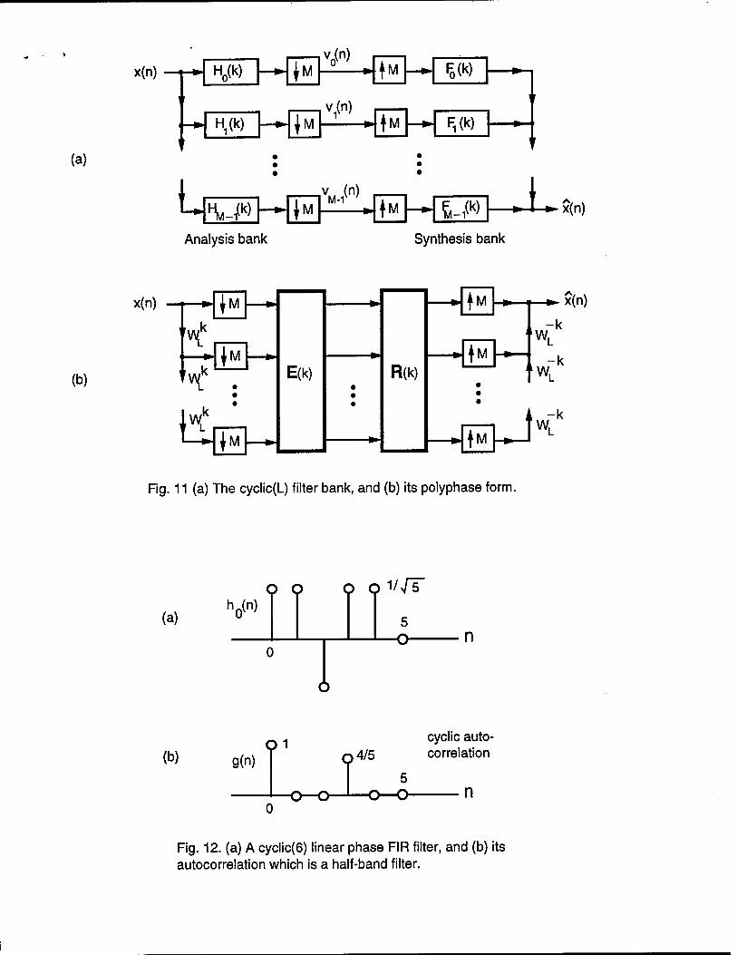
The next example brings out another difference between cyclic and noncyclic filters. Consider a cyclic(6)

transfer function

H0(k) = (l + Wk - Wlk + W$k + W?)/y/5,

whose impulse response is shown in Fig. 12(a). We can regard this as FIR in the sense that h(n) is nonzero

only on a subset of points in 0 < n < L — 1. (In the cyclic case this is the only FIR-definition that makes

sense). The symmetry of the impulse response implies the linear-phase property, as explicitly seen from

H0{k) = Wik(-1 +2cos(nk/3) + 2cos(27rfc/3))/v/5

Now consider the magnitude-squared function G(k) = \H0(k)\2, whose cyclic(6) impulse response g{n)

is the cyclic convolution of h0(n) with h(,(-n). By explicit computation one verifies that #(0) = 1 and

5(2) = g(4) = 0 (Fig. 12(b)). That is, g(2n) = 8(n). So the filter G{k) has the half-band property (in the

cyclic(6) sense), and

G(k) + G(3 + k) = 2, 0 < k < 5. (23)

Equivalently H{k) is power symmetric [23] in the cyclic(6) sense:

|2f0(fc)|2 + |ifo(3 + fc)|2 = 2, 0<fc<5. (24)

That is, we have found a cyclic(6) filter Ho(k) which is both linear-phase and power-symmetric. This is not

possible [23] for the noncyclic FIR case.

11

Using the above example we can construct a two-channel cyclic(6) orthonormal filter bank where the

filters are nontrivial linear phase filters. (Such constructions are not possible in the noncyclic FIR case [23].)

For this choose ho(n) as above, and the remaining three filters as

/U(n) = (-1)»Ä5(1 - n), A(n) = ÄJE(-n) (25)

for k = 0,1, with all arguments interpreted modulo-6. That is, Hx{k) = -W£H$(k - K) where K = L/2,

and Fi(k) = H*(k). The preceding is an example of a cyclic(6) version of the CQF design of Smith and

Bamwell [18].

More on the CQF Design

Given a cyclic(L) impulse response g(n) with the property that G(k) > 0, we can construct infinitely many

cyclic(L) two channel orthonormal filter banks by choosing

ff0(fc) = eM*)yG(fc), (26)

and the remaining three filters according to (25). We can regard H0(k) as a cyclic spectral factor of G(k).

Recall that for noncyclic FIR filters, the usual definition of spectral factors allows only finitely many phase

responses, and the spectral factors all have the same length N + l. In Eq. (26) however, the phase response

<p{k) of the spectral factor H0(k) is arbitrary. In particular, the choice <f>(k) = 0 would yield linear phase

analysis filters H0(k) and Hi(k) with good frequency responses (if G(k) is a good lowpass filter). However,

even if G(k) is cyclic(L) FIR (in the sense that g{n) = 0 for N < n < L - N; see Fig. 13) the cyclic spectral

factor Ho(k) may not be FIR (i.e., ho(k) could be nonzero for all n). An open question here is, what is the

most general form of the phase response (f>(k) which ensures that H0(k) is FIR (possibly with length JV +1)?

A related question is for a given G(k), what is the minimum-length linear-phase spectral factor?

5. THE PARAUNITARY INTERPOLATION PROBLEM

Given an arbitrary cyclic(L) paraunitary system H(fc), that is, a sequence ofMxM unitary matrices

H(0),H(1),...,H(L-1), (27)

can we always find a paraunitary interpolant? That is, can we find a system Hint(eju) = J2n h(n)e-Jwn, such

that its samples at the unit circle points z = W£k agree with H(fe)? This is the paraunitary interpolation

problem. For the scalar case (M = 1) this becomes the allpass interpolation problem. For the matrix case

(arbitrary M) we distinguish between the FIR interpolation problem where Hj„t(z) = ]Cn=0h(n)z-n, and

the IIR case. In the IIR case we again distinguish between rational interpolants (where each element in

12

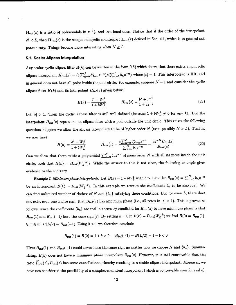
Hint(z) is a ratio of polynomials in z'1), and irrational ones. Notice that if the order of the interpolant

N < L, then Hint(z) is the unique noncyclic counterpart H„c(z) defined in Sec. 4.1, which is in general not

paraunitary. Things become more interesting when N > L.

5.1. Scalar Allpass Interpolation

Any scalar cyclic allpass filter H(fc) can be written in the form (15) which shows that there exists a noncyclic

allpass interpolant Hint{z) = (c£n=o&J-n*"")/(£n=o &"*-") where \c\ = 1. This interpolant is IIR, and

in general does not have all poles inside the unit circle. For example, suppose JV = 1 and consider the cyclic

allpass filter H(k) and its interpolant Hint{z) given below:

Let |6| > 1. Then the cyclic allpass filter is still well defined (because 1 + bW£ ^ 0 for any k). But the

interpolant Hint{z) represents an allpass filter with a pole outside the unit circle. This raises the following

question: suppose we allow the allpass interpolant to be of higher order N (even possibly N > L). That is,

we now have

H{k)==TTW£ Hint{z)- ESLoM-" " BW) ( }

Can we show that there exists a polynomial £n=o bnz~n of some order N with all its zeros inside the unit

circle, such that H{k) = Hint{W£k)l While the answer to this is not clear, the following example gives

evidence to the contrary.

Example 1. Minimum phase interpolants. Let B(k) = 1 + bWl with b > 1 and let Bint(z) = £„=o bnZ~n

be an interpolant B(k) = Bint{W£k). In this example we restrict the coefficients bn to be also real. We

can find unlimited number of choices of N and {bn} satisfying these conditions. But for even L, there does

not exist even one choice such that Bint{z) has minimum phase (i.e., all zeros in \z\ < 1). This is proved as

follows: since the coefficients {6n} are real, a necessary condition for Bint(z) to have minimum phase is that

Bint(l) and Bint(-l) have the same sign [2]. By setting k = 0 in B(k) = Bint(W[k) we find B(0) = Bint{l).

Similarly B(L/2) = Bint{-1). Using b > 1 we therefore conclude

Bint(l) = -B(O) = 1 + b > 0, Bint(-l) = B(L/2) = 1 - 6 < 0

Thus Bintil) and Bint{—1) could never have the same sign no matter how we choose N and {bn}. Summa-

rizing, B(k) does not have a minimum phase interpolant Bint(z). However, it is still conceivable that the

ratio Bint(z)/'Bint(z) has some cancellations, thereby resulting in a stable allpass interpolant. Moreover, we

have not considered the possibility of a complex-coefficient interpolant (which is conceivable even for real b).

13

5.2. FIR Paraunitary Interpolation

Given the unitary sequence (27), can we always find &MxM paraunitary interpolant restricted to be FIR,

i.e., of the form Hint(z) = En=oh(n)z"n? For the scalar case (M = x)the answer is evidently no, because

the interpolant has to be an FIR allpass function (which cannot be more general than a mere delay). So

we assume M ^ 1. If we make the restriction N < L the coefficients h(n) are simply the inverse DFT

coefficients of Hint{W[k) and the interpolant is the noncyclic counterpart defined in Sec. 4.1. This may not

be paraunitary as seen from the examples of Sec. 4.1. More generally, suppose we allow N to be arbitrarily

large but finite. Does this allow us to always find a paraunitary interpolant? In general the answer is still

no, as we shall demonstrate. For this we first review a well know result for noncyclic 2x2 causal FIR

paraunitary matrices [23]:

Theorem 1. Let Hnon(z) = 52n=o Hn)z~n be a 2 x 2 causal FIR system. Then it is paraunitary if and

only if it has the form

Hnon(z) = (30) 'H0(z) eiez-noHi(z) ' Hi{z) -eJ0z-noHo(z).

where H0(z)H0{z) + Hi{z)Hi{z) = 1 (power complementary property), 6 is real, and n0 is any integer large

enough to ensure causality. 0

A proof is included in Appendix C for completeness. Consider now the cyclic(L) example

H(fc) = VQ(fc) o

0 e^fe) (31)

which is evidently paraunitary for any arbitrary (real-valued) a(k) and ß(k). Suppose there exists a noncyclic

causal FIR paraunitary interpolant Hint(z)- If this interpolant is diagonal, then H0(eju) = ce~juN and a(k)

has to be of the form -2nkN/L plus a constant. Thus for arbitrary a(k) and ß{k), there is no diagonal

FIR paraunitary interpolant Hint(z). How about a nondiagonal interpolant? Since it would have the form

(30), a(k) and ß(k) cannot have arbitrary combinations of values. Only those combinations which satisfy

the property

ß(k) = -a(fc) - 27rfcno/L + 6

for some S are allowed. This shows that cyclic paraunitary systems do not in general have noncyclic FIR

paraunitary interpolants. Whenever such an interpolant does exist, it can be factorized into the form [23]

Hint(z) = Hi„t(l) (i - uxuj + z-VuJ) (i - u2u| + z-1u24) ... (i - ujuj + z^ujuty (32)

where u* are unit norm vectors. By replacing z_1 with W£ we obtain

H(fc) = H(0) (i - ui4 + Wtmul) (i - u2u} + W£u24) • • • (i - ujuj + w£uju\) (33)

14

which is a factorization of the cyclic paraunitary system H(fe) in terms of the building blocks [I - u^ +

W^UiuJ). Thus, whenever a noncyclic FIR paraunitary interpolant exists, the cyclic system can be factored

as above. Conversely, if the cyclic system can be factored as in (33), then replacing Wj? with z-1 we obtain

a FIR paraunitary interpolant. Summarizing we have proved:

Theorem 2. FIR interpolants. Let H(fc) be a cyclic(L) paraunitary system, (i.e., H(fc) unitary for

0 < k < L - 1). Then it has a noncyclic causal FIR paraunitary interpolant Hint(z) if and only if H(fc) can

be factorized in the form (33) where u* are unit-norm vectors. 0

5.3. IIR Paraunitary Interpolation

If we do not restrict the interpolant to be FIR, then we can always find a paraunitary interpolant for the

unitary sequence (27). For this we simply define,

IW*)-HM, 2f<»<2-^ (34)

for 0 < k < L - 1. Then the sampled values Hint(W£k) are evidently equal to H(fc). The interpolant

Hint(eJu;) is a piecewise constant, and has discontinuities at the frequencies 2nk/L. It is therefore not a

rational function in eiu (i.e., the elements in the matrix are not ratios of polynomials in z). The following

theorem asserts that we can always construct rational solutions in the IIR case. Stability of the interpolant,

however, is not asserted.

Theorem 3. IIR interpolants. Let H(0), H(l),... H(L - 1) be a sequence of M x M unitary matrices.

Then there exists a causal system with rational transfer matrix Hint(z) such that Hint(W£ ) = H(fc). 0

Proof. The crucial building block is the matrix

Ufc(z)=I - uut + z-1Ffc(z)uut

where Fk(z) is a rational allpass filter and u is a unit-norm vector. We can verify that Ufc(z) is paraunitary,

that is, TJk(z)Ufc(z) = I. Suppose the allpass filter Fk(z) is chosen such that

Fk(W-m) = fwr m^k

We can regard Fk(z) as a rational allpass interpolant (Sec. 5.1) with samples at z = WLm as specified

above. With this choice of Ffc(z), the matrix Ufc(z), sampled at z = W[m, yields

TT fu/~m\ - j1 for all m ^ A; vk(wL )-d_2uut iorm = k

15

Now any M x M unitary matrix can be expressed as a product of M - 1 matrices of the form I - 2uu'.

More precisely [23] each matrix H(fe) in the given unitary sequence can be expressed as

H(fc) = (i - 2ui,fcuJ>fc) (i - 2u2,fcuJtfc) • • • (l - 2uM-i,fcuL-i,fe) A(fc)

where uiifc are unit-norm vectors and A(fc) is diagonal with nth diagonal element e>°k'n. We can find a

rational allpass filter Fn(z) such that

Then the diagonal matrix Dfc(z) with diagonal elements Fn(z) has the unit-circle samples

Dfc(W7m) = |A(jfc) Z = k.

By multiplying matrices of the form Ufc(z) and Dfc(z), we can define a noncyclic paraunitary system Gfc(z)

such that

Gk(WL )-jH(fc) m = k

The product Hint(z) = G0(z)Gi(z)... GL_i(z) then represents a rational IIR paraunitary interpolant for

the given matrix sequenence {H(fc)}. V V V

5.4. Summary of Interpolants and Factorizability

It is well known that noncyclic FIR paraunitary systems can be factored [23] in terms of the building blocks

I - UiuJ + z_1Ujut, where u] Uj = 1. But in the cyclic case, factorization in terms of (I - UJUJ + W^UJUJ) is

not always possible. In fact Theorem 2 shows that such factorization is possible if and only if there exists an

FIR paraunitary interpolant. However, the fact that there always exists a rational IIR interpolant (Theorem

3) means, in particular, that we can obtain a factorization of the cyclic system H(k) in terms of slightly

modified building blocks. These have the form Ufc(z) and Dfc(z) discussed above, with z-1 replaced by W£

everywhere.

6. STATE SPACE DESCRIPTIONS FOR CYCLIC LTI SYSTEMS

In Sec. 2.1 we considered cyclic difference equations, and recursive structures for cyclic transfer functions.

State space descriptions allow us to generalize these ideas. From the direct-form structure of Fig. 6 we can

identify a set of N state variables Vi(n) (outputs of the unit delay elements W£) and obtain equations of the

v(n + 1) = Av(n) + Bx(n) (35)

y(n) = Cv(n)+Dx(n),

16

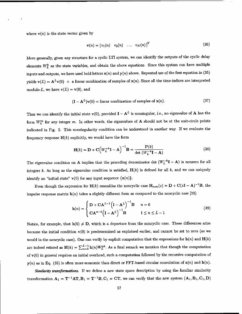
where v(n) is the state vector given by

v(n) = [vi(n) v2{n) ... vN(n)]T (36)

More generally, given any structure for a cyclic LTI system, we can identify the outputs of the cyclic delay

elements W£ as the state variables, and obtain the above equations. Since this system can have multiple

inputs and outputs, we have used bold letters x(n) and y(n) above. Repeated use of the first equation in (35)

yields v(L) = ALv(0) + a linear combination of samples of x(n). Since all the time-indices are interpreted

modulo-X, we have v(L) = v(0), and

(I - AL)v(0) = linear combination of samples of x(n). (37)

Thus we can identify the initial state v(0), provided I - AL is nonsingular, i.e., no eigenvalue of A has the

form W£* for any integer m. In other words, the eigenvalues of A should not be at the unit-circle points

indicated in Fig. 2. This nonsingularity condition can be understood in another way. If we evaluate the

frequency response H(fc) explicitly, we would have the form

HW,D + c(^.-A)-B.det(;W.A) (38)

The eigenvalue condition on A implies that the preceding denominator det (W£kI - A) is nonzero for all

integers k. As long as the eigenvalue condition is satisfied, H(fc) is defined for all k, and we can uniquely

identify an "initial state" v(0) for any input sequence {x(n)}.

Even though the expression for H(fc) resembles the noncyclic case Hnon(z) = D + C(zl - A)_1B, the

impulse response matrix h(n) takes a slightly different form as compared to the noncyclic case [23]:

D + CA^"1 (l - ALN _1

h(n) = i D + CA^-1 (l - AL) B n = 0

V - / (39) CA^Tl-A1) XB l<n<L-l

Notice, for example, that h(0) ^ D, which is a departure from the noncyclic case. These differences arise

because the initial condition v(0) is predetermined as explained earlier, and cannot be set to zero (as we

would in the noncyclic case). One can verify by explicit computation that the expressions for h(n) and H(fc)

are indeed related as H(fc) = XIn=o h(n)W£fc. As a final remark we mention that though the computation

of v(0) in general requires an initial overhead, such a computation followed by the recursive computation of

y(n) as in Eq. (35) is often more economic than direct or FFT-based circular convolution of x(n) and h(n).

Similarity transformations. If we define a new state space description by using the familiar similarity

transformation Ai = T_1AT,B! = T_1B,Ci = CT, we can verify that the new system (Ai,Bi,Ci,D)

17

, -1

x(n - 2)

x(n — L).

(40)

has the same h(n). Reason: we can verify by substitution that CAB_1(l - AL) B is unchanged by

the similarity transform for any n > 1. Thus we can find equivalent cyclic state space realizations by using

similarity transforms. Note that even though D does not represent h(0), it is still unchanged in the similarity

transformation.

6.1. Reachability and Observability

The ideas of reachability and observability [6], [9], [23] can be extended to cyclic LTI systems but there are some

differences from the traditional noncyclic case. For example we will see that reachability and observability

together do not imply minimality. The cyclic LTI system is said to be reachable if we can arrive at any

chosen final value v/ for the state vector v(n) at any chosen time n by proper choice of the input sequence

x(.). To quantify this consider the state recursion v(n +1) = Av(n) + Bx(n) again. If we apply this L times

and use the periodicity conditions v(n + L) = v(n) and x(n + L) = x(n) we find

■ x(n - 1)'

(I - AL)v(n) = [B AB ... A^B]

11A,B(.L)

Here we have used the notation that for any positive integer i,

ft,U»(*)=[B AB ... A-XB] (41)

Let N denote the state dimension (size of v(n)) and r the number of inputs (size of x(n)). Then HA,B{i)

is a N x ir matrix with rank < N. The matrix TZA,B(L), in particular, has size N x Lr. Assume (I - AL)

is nonsingular for reasons explained earlier. It is then clear that we can attain any value for the state v(n)

at any time n by application of a suitable input x(n - l),x(n - 2),... ,x(n - L) if and only if the matrix

TIA,B{L

) has rank N- Tnis Sives a test for reachability. Now two cases should be distinguished:

1. Let N < L. Then the rank of KA,B(N

) wil1 be e<*ual to that of nA,B(L) (Cayley-Hamilton theorem).

Then the reachability test reduces to the conventional one. Moreover, in the nonreachable case we can

perform the usual reduction and reduce the size N of the state vector.

2. Let N > L. This is possible in the mimo case (e.g., if H(fc) = W£lr, then N = r regardless of L). For

this case two subcases are possible:

2.1. The rank of TIA,B{L) is already N, so the system is reachable.

2.2. The rank of KA,B{L) is smaller than that of KA,B{N). If the latter is also less than N, we can

perform the usual reduction and reduce the size N of the state vector. If the rank of UA,B{N) is

already N, we cannot do this, but we might still be able to perform a reduction of the cyclic state

space equations as we shall demonstrate below.

18

State-observability in a cyclic LTI system can also be defined similar to the traditional case, but with some

subtle distinctions between the cases N < L and N > L. First assume N < L. The output equation

y(n) = Cv(n) + Dx(n) can be repeatedly applied to yield

y(n) y(n + l)

y{n + N-l)

C CA

CA N-l

v(n) + func. of x(n), x(n + 1),... x(n + N - 1) (42)

SC,A(")

The initial state v(n) can be uniquely found from the JV samples of the input and output in this equation,

as long as the matrix SC,A(N

)> which has N columns, has rank N. If N > L, the preceding equation is

not meaningful because y(i) and x(i) repeat with period L. In this case, however, we have a very unusual

situation. If the input and output are known for all L values of time, then in particular x(i) is known for

all i and we can identify the state v(n) for all n using the state recursion. Thus the notion of observability

becomes trivial for N > L.

Example 2

Consider the cyclic system

,L-lTi/(£-l)k H(k) = 1 + aWl + a2Wr + ... + o^"1^ (43)

for which a direct-form implementation is shown in Fig. 14(a). With state variables as indicated, the state

space description (A, B, C, D) can readily be identified, yielding

0 1 0 0 0 1

0 0 0 0 0 0

B = C = fo- L-l ,L-2 D = \ (44)

Note that the number of state variables N = L-l. From the preceding we verify that

KAML) =

0 0 0 0

0 1 1 0

0 10 10 0

0 0 0 0 0 0

SC,AW = 0

0

lL-2

■.L-l a

,L-1

(45)

Since N = L - 1, TZA,B(L) has size (L-l)xI and SC,A(N

) has size (L - 1) x (L - 1). Both of these

matrices have rank N = L - 1 (assuming, of course, a ^ 0), showing that the structure is both reachable

and observable. Notice, however, that the system H(k) can be rewritten in the recursive form

H(k) \-aL

1-oWj (46)

19

using the fact that W£ = 1. This yields the simpler recursive implementation requiring only one cyclic delay

W£ (Fig. 14(b)). We can verify that the state space description of the simplified structure is

A = a, 5 = 1, C = a(l-aL), D = l-aL (47)

In this case the number of state variables N = 1. One readily verifies that UA,BO-) = 1 and SC,A(1) = a(! ~

aL). So KA,B{L) and SC,A(N

) have rank N, and the structure is reachable and observable (assuming a ^ 0

and aL ^ 1). Thus the two structures shown in Fig. 14 are two reachable and observable implementations of

H{k) with different state dimensions! The first one requires L - 1 cyclic delays (the W£ elements) whereas

the second structure requires only one cyclic delay. Notice also that the quantity D is different for the two

structures unlike noncyclic systems. This is consistent with the fact that for cyclic systems h(0) ^ D but is

given by the more elaborate expression (39).

Example 3

Consider the 2 x 2 cyclic system shown in Fig. 15(a), and assume L = 3. The number of state variables is

N = 4. The state space description has

A =

Then explicit computation shows that

0 1 0 01 ro on 0 0 10 0 0 0 1

, B = 1 1 0 0 , c =

0 o o oj Li IJ

0 0 10 10 0 0

(48)

nA,B(L)

ro o l l o o 110 0 11 0 0 110 0

Ll 1 0 0 0 0

, nAtB{N) =

ro o l l o o l l 110 0 110 0 00110000 1100000 0

ScA*)

0 0 10 10 0 0 0 0 0 1 0 10 0

Thus TZA,B{L) has rank 3 < N which shows that the cyclic system is not reachable. However, 11A,B(N)

has rank 4. Since SC,A(?) nas rank 4' so does SC,A(

N)-

SO we cannot perform state-reduction using classical

techniques. In this example, however, it is possible to perform state reduction of the cyclic system by simple

manipulations of the structure, and by using the fact that W^ = 1. For this we notice the identity

1 1 1 1

1 0 0 x

1 1 1 1

= (l+x)

which shows that the transfer matrix of Fig. 15(a) is eventually

"1 + Wf

1 1 1 1

H(*) = 0 0

w?k + w£ l l l l

l + Wj*

wg + wik [i i] (49)

which has the implementation shown in Fig. 15(b) requiring only two cyclic delays. Thus in this example,

R-A,B(N) and SC,A(N

) nave rank N but ^A,B(L) does not, and we have been able to reduce the state

dimension.

20

In Example 2 we found that the state dimension could be reduced even though the cyclic system is

reachable as well as observable. In Example 3 we found that HA,B{N

) and SC,A(

N)

have rank N and

T^A,B{L) has deficient rank, and the state dimension could again be reduced. The question now is, what is a

necessary and sufficient condition for the minimality of state dimension in cyclic LTI structures? A related

question is, can we develop a theory paralleling the Smith-McMillan form and relate the minimum state

dimension (McMillan degree) to this form? These appear to be fundamental questions requiring future work.

6.2. Unitariness of Realization Matrix

Suppose we are given an implementation for a cyclic transfer matrix E(k). This implementation has a state

space description of the form (35). The realization matrix for the implementation is defined as

A B C D

The following result connects the cyclic-paraunitary property to unitariness of the realization matrix.

Lemma 1. If the realization matrix is unitary, then the cyclic system E(fc) is paraunitary.

Proof. Rewrite the state equations as

(50)

"v(n + l)" y(n)

= A B C D

'v(n)' x(n)

Unitariness of the realization matrix implies ||v(n+1)||2 + ||y(n)||2 = ||v(n)||2 + ||x(n)||2 where ||v||2 denotes

vl v. If we write the preceding equation for 0 < n < L — 1 and add them up, we obtain

L-l L-l

^yt(n)y(n) = ]£xt(n)x(n) n=0 n=0

by using the fact that v(n + L) = v(n). With X(fc) = J2nZl x(n)W£fe and Y(fc) = £^o y(n)W£k, we then

obtain (using Parseval's relation) J^kZo Yt(fc)Y(fc) = Efc=oxt(fc)x(A:)' that is>

L-l L-l

53 xt(fc)Et(Jfc)E(fc)X(Jb) = ]Txt(fc)X(fc) fc=0 fc=o

This should hold for all sequences {X(A;)}, which implies that xt(fc)Et(fc)E(fc)X(fc) = xt(fe)X(fe) for any

X(jfc), proving Et(fc)E(fc) = I indeed. V VV

This result is analogous to a result in the noncyclic case [23]. However, unlike in the noncyclic case,

we do not have the converse result. That is, even if E(A;) is paraunitary, there may not exist a minimal

nonrecursive structure (i.e., minimal structure with all eigenvalues of A equal to zero), with unitary system

matrix. When such a structure does exist, the FIR interpolant Ejnt(z) = D + C(zl - A)_1B, obtained by

21

replacing W£ with z-1 in the structure, would be paraunitary (because a result like Lemma 1 also holds

in the noncyclic case [23]). Since FIR paraunitary interpolants do not always exist (Sec. 5.2), the point is

proved. By combining this observation and Theorem 2 we obtain the following result.

Theorem 4. Let E(fc) be cyclic paraunitary. Then the following statements are equivalent.

1. There exists a causal FIR paraunitary interpolant 'Eint{z).

2. E(fc) can be factorized into unitary building blocks as in (33).

3. There exists a cyclic implementation of E(fc) such that the realization matrix is unitary. 0

7. CONCLUDING REMARKS

The main purpose of this paper has been to introduce the idea of cyclic LTI systems, place in evidence some

interesting theoretical properties, and point out a few open problems. The emphasis has primarily been on

cyclic versions of recursive difference equations, allpass filters, paraunitary matrices, multirate filter banks,

and state space theory. It will be interesting to figure out how to exploit the extra freedom offered by the

cyclic system, e.g., for the design of subband coders. Can this be exploited to obtain increased coding gain

(or compression), or to reduce the complexity of implementations? Evidently more work is necessary in order

to assess the practical advantages. We saw that cyclic LTI systems open up interesting problems in the more

general area of signal and system theory. Many of these were mentioned throughout the paper. One can

also attempt to formulate cyclic versions of other standard problems in filter bank theory, for example cosine

modulated filter bank design. The important thing again would be to establish a clear advantage for such

extensions.

Appendix A. Proof of cyclic-decimation formula

By definition the output of the cyclic decimator is

y{n) = x{Mn) = ± £ X(m)W£m{Mn) = \ £ X(m)W«mn

m=0 m=0

1 K-\ M-l 1 K-l - M-l

= T E WKkU E X(Ki + k) = i E Vrf'ji E X(Ki + k) fe=0 »=o fc=o »=o

So the ff-point DFT of y(n) is E^1 X{Ki + k)/M, or equivalent^ S^'1 X(k - iK)/M.

Appendix B. Cyclic alias-component matrix

Using the decimator and expander formulas (7) and (9) we can express the L-point DFT of the reconstructed

signal x(n) as M-l M-\ -

X(k) =Y^x(k~ iK) E MHm{-k ~ iK)Fm(k)> 0 < fc < L - 1, i=0 m=0

22

where K = L/M. The alias components are X{k - iK),i ^ 0, and the desired signal term is X(k). So the

perfect reconstruction condition is

H(fc)

F0(k) F1(k)

M' 0

0 ■ FM-i(k).

where H(fc) is the alias component (AC) matrix with (i,m) element [H(/c)]im = Hm(k - iK). Now the

analysis filters and polyphase matrix are related as

[H0(k) H,(k) ... HM.1{k)] = [l WkL ... wiM-1)k]ET(k)

Using the fact that E(fc) is periodic^), we can show that H(fc) = W^A(fc)ET(fc) where W« is the

M x M DFT matrix, and A(/c) is diagonal with ith element Wik. Thus orthonormality (unitarity of E(fc))

is equivalent to H'(fe)H(A;) = MI. In the two channel case the cyclic AC-matrix is

H0(k) H^k)

ßo(k-K) H^k-K)^

where K = L/2. If H0(k) satisfies the cyclic power symmetry property \H0(k)\2 + \H0(k - K)\2 = 2, and if

.ff^jfe) = —W^H^k - K) we can verify by substitution that H'(/c)H(fc) = 21, and the cyclic filter bank is

indeed orthonormal. Finally, the theory of alias-free filter banks (i.e., the pseudocirculant conditions [23])

can be extended to the cyclic case in a straightforward manner, so we skip the details.

Cyclic orthonormal basis. For orthonormal cyclic filter banks with perfect reconstruction R(/c) is also

unitary, so the matrix F(fc) whose elements are [F(fc)]rm = Fm(k - rK) also satisfies F'(fc)F(fc) = MI,

that is, Y^Fiik - rK)F^{k - rK)/M = 8{i - m). The left hand side is the .fiT-point DFT of the

M-fold decimated version of g{i)=Y^n=o /»(n)/m(n - ^)- Thus orthonormality of R(fc) is equivalent to

En^o /i(")/m(" - Mi) = S(i - m)8{l) which proves (19).

Appendix C. Proof of Theorem 1

The FIR matrix H(z) is of the form H(z) Since the "if" part is obvious, we concentrate Ho(z) G0(z) H^zJ Gi(z)_

on the "only if" part. The paraunitary property H(z)H(z) = I implies, among other things, that

H0(z)H0(z) + H1(z)H1(z) = l

Ho(z)Go(z) + H1(z)G1(z) = 0

(51)

(52)

Suppose an element in H(z) is identically zero, e.g., H\(z) = 0 for all z. Then Ho(z)Go(z) = 0 for all z, from

(52). Since HQ(Z) is nonzero from (51), we conclude Go(z) = 0 for all z. Thus the FIR paraunitary matrix

23

H(z) becomes diagonal, proving the desired form (30). So we assume that none of the four elements in

H(z) is identically zero. Now, any pair of power complementary transfer functions (i.e., a pair H0{z), Hi{z)

satisfying (51)) should be free from nontrivial common factors (i.e., factors other than cz~n°), because the

left side of (51) should be nonzero for all z. So H0(z) and Hx{z) have no nontrivial common factors. The

same holds for the pair G0(z) and Gx(z) and the pair H0(z) and Hi(z). So from Eq. (52) we conclude

G0(z) = coz-^Hiiz), Gi(*) = clZ-n'H0(z)

which upon substitution into Eq. (52) yields (coz-"0 +c1z-ni)H0(z)H1(z) = 0 proving coz""0 +0^-^ = 0.

Thus co = -ci, and n0 = m. Since the row elements H0{z) and G0(z) are also power complementary, i.e.,

H0(z)H0(z) + G0(z)G0{z) = 1, we get H0(z)H0(z) + |co|2.ffi(z)tfi(z) = 1. Comparing this with (51) we

conclude |co|2 = 1, i.e., CQ = eje. This establishes the form (30). V VV

References

[1] Akansu, A.N., and Haddad, R.A., Multiresolution signal decomposition: transforms, subbands, and

wavelets, Academic Press, Inc., 1992.

[2] Antoniou, A. Digital filters: analysis and design, McGraw Hill Book Co., 1979.

[3] Bopardikar, A. S., Raghuveer, M. R., and Adiga, B. S. "Perfect reconstruction circular convolution filter

banks and their applications to the implementation of bandlimited discrete wavelet transforms", Proc.

IEEE Int. Conf. Acoustics, Speech, and Signal Processing, pp. 3665-3668, Munich, May 1997.

[4] Bopardikar, A. S., Raghuveer, M. R., and Adiga, B. S. "PRCC filter banks: theory, implementation,

and application", Proc. SPIE., vol. 3169, San Diego, CA, July-Aug 1997.

[5] Caire, G., Grossman, R. L., and Poor, H. V. "Wavelet transforms associated with finite cyclic groups,"

IEEE Trans, on Information theory., pp. 1157-1166, July 1993.

[6] Chen, C. T. Linear system theory and design, Holt, Rinehart, and Winston, Inc., 1984.

[7] de Queiroz, R. L., and Rao, K. R. "On reconstruction methods for processing finite-length signals with

paraunitary filter banks", IEEE Trans. Signal Proc, pp. 2407-2410, Oct. 1995.

[8] Gold, B. and Rader, C. M. Digital processing of signals, McGraw Hill Book Co., NY, 1969.

[9] Kailath, T. Linear Systems, Prentice Hall, 1980.

[10] Karlsson, G. and Vetterli, M. "Extension of finite length signals for subband coding," Signal Processing,

vol. 17, pp. 161-168, June 1989.

[11] Kiya, H., Nishikawa, K., Sagawa, M. "Property of circular convolution for subband image coding,"

IEICE Trans. Fundamentals, vol. E75-A. No. 7, pp. 852-860, July 1992.

24

[12] Malvar, H. S. Signal processing with lapped transforms, Artech House, Norwood, MA, 1992.

[13] Motwani, R., and Ramakrishnan, K. R. "Design of two channel linear phase orthogonal cyclic filter

banks", IEEE Signal Processing Letters, pp. 121-123, May 1998.

[14] Nishikawa, K., Miyazaki, K., and Kiya, H. "A parallel AR spectral estimation using a new class of filter

bank", Proc. IEEE Int. Conf. Acoustics, Speech, and Signal Processing, pp. 244-247, April 1993.

[15] Nuri, V., and Bamberger, R. H. "Size-limited filter banks for subband image compression", IEEE Trans.

Image Proc, pp. 1317-1323, Sept. 1995.

[16] Nussbaumer, H. J. "Digital filtering using polynomial transforms," Electronics Letters, vol. 13, pp.

386-387, 1977.

[17] Oppenheim, A. V., and Schäfer R. W. Discrete time signal processing, Prentice Hall, 1989.

[18] Smith, M. J. T., and Barnwell III, T. P. "Exact reconstruction techniques for tree-structured subband

coders," IEEE Trans, on Acoustics, Speech and Signal Proc, pp. 434-441, June 1986.

[19] Smith, M. J. T., and Eddins, S. L. "Analysis/synthesis techniques for subband image coding," IEEE

Trans, on Acoustics, Speech and Signal Proc, vol. ASSP-38, pp. 1446-1456, Aug. 1990.

[20] Roberts, R. A., and Mullis, C. T. Digital signal processing, Addison-Wesley Publ. Co., 1987.

[21] Strang, G. and Nguyen, T. Wavelets and filter banks, Wellesley-Cambridge Press, 1996.

[22] Vaidyanathan, P. P., and Liu, V. C. "Efficient reconstruction of bandlimited sequences from nonuni-

formly decimated versions by use of polyphase filter banks," IEEE Trans, on Acoust. Speech and Signal

Proc, vol. ASSP-38, pp. 1927-1936, Nov. 1990.

[23] Vaidyanathan, P. P. Multirate systems and filter banks, Prentice Hall, 1993.

[24] Vaidyanathan, P. P., and Kirac, A. "Theory of cyclic filter banks" Proc. IEEE Int. Conf. Acoustics,

Speech, and Signal Processing, pp. 2449-2452, Munich, May 1997.

[25] Vaidyanathan, P. P., and Kirac, A. "Cyclic systems and the paraunitary interpolation problem", Proc.

IEEE Int. Conf. Acoustics, Speech, and Signal Processing, pp. 1445-1448, Seattle, May 1998.

[26] Vaidyanathan, P. P. "Results on cyclic signal processing systems" Proc. EUSIPCO, Island of Rhodes,

Greece, Sept. 1998.

[27] Vetterli, M., and Kovacevic, J. Wavelets and subband coding, Prentice Hall, Inc., 1995.

25

List of Figures

Fig. 1. A cyclic LTI system.

Fig. 2. The points on the unit-circle corresponding to the DFT frequencies {L = 8).

Fig. 3. Two ways to represent a cyclic(L) delay.

Fig. 4. The direct-form implementation of an arbitrary cyclic(L) LTI system.

Fig. 5. The cyclic direct-form structure for a first order filter.

Fig. 6. The cyclic direct-form structure for a iVth order filter.

Fig. 7. (a) M-fold decimation of cyclic(L) input, (b) example of a cyclic(6) input, and (c) 2-fold

decimated version.

Fig. 8. (a) M-fold expander for cyclic(K) input, (b) example of a cyclic(3) input, and (c) 2-fold expanded

version.

Fig. 9. (a) A decimation filter, (b) cyclic-polyphase form, and (c) simplification using cyclic noble

identity.

Fig. 10. Noble identities for cyclic multirate systems, (a) Polyphase component before decimator, and

(b) polyphase component after decimator.

Fig. 11. (a) The cyclic(L) filter bank, and (b) its polyphase form.

Fig. 12. (a) A cyclic(6) linear phase FIR filter, and (b) its autocorrelation which is a half-band filter.

Fig. 13. (a) A cyclic(£) FIR filter, and (b) its non-FIR spectral factor.

Fig. 14. Example 2. Two implementations of a cyclic(L) system. Both of these are reachable and

observable implementations, (a) L - 1 state variables used, and (b) only one state variable used.

Fig. 15. Example 3. (a) A cyclic(3) system requiring four cyclic delays, and (b) reduced system requiring

two cyclic delays. Classical techniques cannot be used to perform this reduction.

x(n) h(n) y(n)

Fig. 1. A cyclic LTI system.

z-plane

Fig. 2. The points on the unit-circle correspond- ing to the DFT frequencies (L=8).

x(n)

x(n)

W,r y(n)

w; ■y(n)

Fig. 3. Two ways to represent a cyclic(L) delay.

x(n) WL W,r

X X' \7h(o) v7h(1)

x(n) t »

x(n)

• • •

I 5o p

w

y(n)

U}X{M Fig. 5. The cyclic direct-form structure for

a first order filter.

►—(

i

1

1 "~J~~^—' wL

k

. 'b^1 t 1* .

1—►

i

1 q 1/ wL

k

• ' i ' •

.

T • • •

,

|v2(n)

"bN l-TJ aN /I I IS

i

y(n)

N vfn) K

Fig. 6. The cyclic direct-form structure for a Nth order filter.

Fig. 4. The direct-form implementation of an arbitrary cyclic(L) LTI system.

(a) x(n) »

cyclic(L) \M . y(n)=x(Mn)

cyclic(K) L=MK

(b) # • •

ll I liin O x(n)

cyclic(6) input

Lü_L-.'

(c) • •

? ^ > o c > c >

o

T h 1? o

T o

y(n) cyclic(3) output of 2-fold decimator

I • • •

Fig. 7. (a) M-fold Decimation of cyclic(L) input, (b) example of a cyclic(6) input, and (c) 2-fold decimated version.

(a) x(n)

cyclic(K)

fM -► y(n)

cyclic(L) L=MK

(b) • •

0 o

o

T o

IT

1 o

It 0

? ? T 1

x(n) cyclic(3) input of 2-fold expander

I • • •

(c) • •

1 o—•—o-

o y(n)

I—I—0—■—0—'—0—'—(

cyclic(6) output of 2-fold expander

• • •

-I—o-

Fig. 8. (a) M-fold expander for cyclic(K) input, (b) example of a cyclic(3) input, and (c) 2-fold expanded version.

H(k) JM

(a)

» •

w:

w,r

wr

EM

^Hl

\M f

{M to i 1

"

SZH1 iM » » »

JM » FW » 9

t wL

k

i r

"

|M -r- F (k) »II

• • •

' ' JM - F (k) to i -u- MV ; * •

(b) (c)

Fig. 9. (a) A decimation filter, (b) cyclic-polyphase form, and (c) simplification using cyclic noble identity.

x(n)

-O—I—O—■—O—■—O—'—O—L

u(n)

Q IDFT (L=6,M=2,K=3)

cyclic(L) Em<k»

cyclic(L) |M v(n)

cyclic(K)

(a)

x(n)

cyclic(L) M

cyclic(K)

In

E (k) m

_vjn)

cyclic(K)

TTITTIT?

/ IDFT (L=6,M=2,K=3)

0

(b)

Fig. 10. Noble identities for cyclic multirate systems, (a) Polyphase component before decimator, and (b) polyphase component after decimator.

(a)

Wrri - .

Ho(k) —»- ^M 0' ' |M —*> F0(k) x(n) —i

< ' ' v(n) M,(k) —► |M

V ' |M F,(k)

' ' <

Ü v (n)

»W» JM M-l fM Uk> Analysis bank

x(n)

Synthesis bank

(b)

x(n) |M

W —^

tv\£ JM

JM

E(k) R(k)

|M

fM

x(n)

W,

-k W,

rm twLk

Fig. 11 (a) The cyclic(L) filter bank, and (b) its polyphase form.

(a)

Q Q Q Q 1/>/T hQ(n)

5 -O n

(b) 01

9(n)

-o—o 1 4/5

cyclic auto- correlation

5 -O—O n

Fig. 12. (a) A cyclic(6) linear phase FIR filter, and (b) its autocorrelation which is a half-band filter.

-) 0 Ä FIRg(n)

(a) liiJiiuiL 0 N L-N L-1

spectral factor h(n)

(b) TTyy'^VoTf? ■ 0 i~

Rg. 13. (a) A cyclic(L) FIR filter, and (b) its non-FIR spectral factor.

<(n) _ WLk VL-In) V\f wf Vl(n)

y y w- y(n) I—» + » —» # »

(a)

1-al

(b)

Fig. 14. Example 2. Two implementations of a cyclic(L) system. Both of these are reachabale and observable implementations, (a) L-1 state variables used and (b) only one state variable used.

wk **3

wk

v2(n) v,(n)

state variables

(b)

x0(n)

x/n)

1 I

w3k - wk

» (

W3 '

Vn(n)

^(n)

Fig. 15. Example 3. (a) A cyclic(3) system requiring four cyclic delays, and (b) reduced system requiring two cyclic delays. Classical techniques cannot be used to perform this reduction.

FOOTNOTES

1. Manuscript Received

2. Work supported in parts by the Office of Naval Research Grant N00014-93-1-0231, and Tektronix, Inc.

3. The authors are with the Department of Electrical Engineering, California Institute of Technology,

Pasadena, CA 91125.