Cryogen Based Energy Storage: Process Modelling and ...

Cryogen Based Energy Storage: Process Modelling and

Optimisation

Yongliang Li

Submitted in accordance with the requirements for the degree of

Doctor of Philosophy

The University of Leeds

Institute of Particle Science and Engineering

School of Process, Environmental & Materials Engineering

September 2011

i

The candidate confirms that the work submitted is his own and that appropriate

credit has been given where reference has been made to the work of others.

This copy has been supplied on the understanding that it is copyright material and

that no quotation from the thesis may be published without proper

acknowledgement.

©< September 2011> The University of Leeds <Yongliang Li>

ii

Acknowledgements

I would like to express profound gratitude to my academic supervisor, Prof. Yulong

Ding, for his invaluable support, endless encouragement, enthusiastic supervision

and useful suggestions throughout this research work. His wide knowledge and his

logical way of thinking have been of great value for me. His moral support and

continuous guidance enabled me to process my work successfully. Going over the

concepts with him again and again was always a distinct pleasure. I am also deeply

indebted to Prof. Haisheng Chen (now with the Institute of Engineering

Thermophysics of Chinese Academy of Sciences) for his detailed and constructive

comments, and for his important support throughout this work.

I wish to express my warm and sincere thanks to Prof. Chunqing Tan from Institute

of Engineering Thermophysics, Chinese Academy of Sciences, who introduced me

to the field of thermodynamics. His ideals and concepts have had a remarkable

influence on my entire career in the research field.

I gratefully acknowledge UK Highview Power Storage Ltd and UK Engineering and

Physical Sciences Research Council (EPSRC) for their three and a half years

financial support through the scheme of a Dorothy Hodgkin Postgraduate Award. I

greatly appreciate the support received through the collaborative work undertaken

with Highview Power Storage Ltd. Very special thanks are also due to the Institute of

Particle Science and Engineering for the provision of a fantastic research

environment. My colleagues in Prof. Ding’s research group have supported me in

various aspects of my research work and living. I want to thank them for all their

help, support, interest and valuable comments. Expressly I am obliged to Dr. Lingling

Zhang, Dr. Yunhong Jiang, Mrs. Hui Cao, Dr. Jianguo Cao, Mr. Yanping Du, Dr.

Sanjeeva Witharana, Mr. Xinjing Zhang and Dr. Christopher Hodges.

Last but not least, a big thank you to my family. My parents Xiumei Fan and Gao Li

are the two most special persons in my life. They, not only gave me life, but also fill it

with all the love and affection one can wish for. A big thank you to my wife Janet

Hong who accomplished without complaints the endless errands that I asked her to

do, even when she was on peaks of stress and lack of sleep because of her studies.

Without her I would be a very different person today, and it would have been much

iii

harder to finish a PhD. Still today, learning to love her and to receive her love makes

me a better person. I also would like to thank my son, Sean, simply for his existence.

One day, he may be able to and inclined to understand what I have written here.

iv

Abstract

Reliable operation of large scale electric power networks requires a balance of

generation and end-user. The electricity markets mainly depend on the real-time

balance of supply and demand because no sufficient power storage is available at

present. As the difference between the peak and off-peak loads is significant, it is

very expensive for the power companies to deal with the demand-supply mismatch.

The situation is getting more challenging with the increasing use of renewable

energy sources particularly wind and solar, which are intermittent and do not match

the actual energy demand. This makes the large scale energy storage and power

management increasingly important.

This thesis studies a Cryogen based Energy Storage (CES) technology which uses

cryogen (or more specifically liquid air/nitrogen) as an energy carrier for large scale

applications in Supply Side Management (SSM). The aim of this research is to seek

the best routes and optimal operation conditions for the use of the CES technology.

A systematic optimisation strategy is established by extending the concept of

‘superstructure’ and combining with Pinch Technology and Genetic Algorithm. Based

on this strategy a program named Thermal System Optimal Designer (TSOD) is

developed to evaluate or optimise both the thermodynamic and economic

performances of thermal systems. Three types of CES systems are proposed and

optimised for the applications of load levelling, peak-shaving and cryogenic energy

extraction.

In the load levelling system it is found that the integration of air liquefaction and

energy releasing process gives a remarkable improvement of the round trip

efficiency. If the expander cycle is used to supply cold energy and the waste heat

with a temperature higher than 600K is available, the round trip efficiency attains to

80 - 90% under rather reasonable conditions. Economic analyses reveal that such a

CES system is very competitive with the current energy storage technologies if the

operation period of the energy releasing unit is longer than 4 hours a day.

In the peak-shaving system CES is integrated with Natural Gas Combined Cycle

(NGCC) to form oxy-fuel combustion for CO2 capture. The optimisation of such

systems gives an exergy efficiency of 70% and electricity storage efficiency of 67%

v

while using helium or oxygen as the blending gas. Economic analyses show that

both the capital and peak electricity costs of the peak-shaving systems are

comparable with the NGCC which are much lower than the oxy-NGCC if the

operation period is relatively short. And the use of helium as the blending gas gives

the lowest costs due to the lowest combustion pressure and mass flowrate.

A new solar-cryogen hybrid power system is proposed to extract cryogenic energy

and to make use of solar radiation for power generation. The system is compared

with a solar thermal power system and a cryogen fuelled power system.

Thermodynamic analyses and optimisation show that the hybrid system provides

over 30% more power than the summation of the power outputs of the other two

systems. The results also suggest that the optimal hot end temperature of the heat

carrier heated by the solar collectors be about 600K for the hybrid system.

Although interesting and promising results are obtained in this study, practical

applications of CES technology meet a number of challenges including the dynamic

operation and economic optimisation of the system in the simulation aspect and

related experimental demonstration for both the key components and the integrated

systems.

vi

Table of Contents

Acknowledgements ..............................................................................ii

Abstract ................................................................................................iv

Table of Contents ................................................................................vi

List of Figures .......................................................................................x

List of Tables.......................................................................................xv

Abbreviations.....................................................................................xvi

Nomenclature....................................................................................xvii

Chapter 1 Background and Motivation............................................1

1.1 Demand for Energy Storage ................................................................. 1

1.1.1 Characteristics of End-users’ Electric Demands ................................... 1

1.1.2 Characteristics of Renewable Energy Resources................................. 5

1.2 Principles and Classifications of Energy Storage Technologies ........... 7

1.3 Cryogenic Energy Storage.................................................................. 11

1.3.1 Exergy Density of Cryogens ............................................................... 12

1.3.2 Storage and Delivery of Cryogens ...................................................... 16

1.3.3 Thermodynamic Properties of Cryogens............................................. 17

1.4 Aim of This Research.......................................................................... 19

1.5 Structure of This Dissertation.............................................................. 19

Chapter 2 Literature Review...........................................................21

2.1 Large Scale Gas Liquefaction............................................................. 21

2.1.1 Cascade Refrigerant Cycle ................................................................. 23

2.1.2 Mixed Refrigerant Cycle...................................................................... 26

2.1.3 Expander Cycle .................................................................................. 29

2.1.4 Summary ............................................................................................ 33

2.2 Cryogenic Energy Extraction Processes............................................. 34

2.2.1 Indirect Rankine Cycle Method ........................................................... 34

2.2.2 Indirect Brayton Cycle Method............................................................ 36

2.2.3 Combined Method .............................................................................. 39

2.2.4 Further Discussion.............................................................................. 42

vii

2.2.5 Summary ............................................................................................ 45

2.3 Hydrogen and Liquid Air/Nitrogen as Energy Carriers ........................ 46

2.3.1 Carrier Production............................................................................... 47

2.3.2 Carrier Storage and/or Transportation ................................................ 48

2.3.3 Energy Extraction of the Carriers........................................................ 50

2.3.4 Summary ............................................................................................ 53

2.4 Summary of the Literature Review...................................................... 54

Chapter 3 Methodologies for Modelling and Optimisation ..........56

3.1 Thermodynamic Modelling.................................................................. 56

3.1.1 Component Modelling......................................................................... 56

3.1.2 Thermodynamic Properties................................................................. 59

3.2 The Pinch Technology ........................................................................ 61

3.2.1 Introduction to the Pinch Technology.................................................. 61

3.2.2 Principle of Pinch Technology............................................................. 63

3.2.3 Systematic Optimisation Using Pinch Technology.............................. 68

3.3 Genetic Algorithm ............................................................................... 72

3.3.1 Introduction to the Optimisation Algorithms ........................................ 72

3.3.2 The principle of GA ............................................................................. 73

3.4 Summary of This Chapter ................................................................... 75

Chapter 4 Integration of CES System with Liquefaction..............77

4.1 Background......................................................................................... 77

4.2 Linde-Hampson CES System ............................................................. 80

4.2.1 Cold Storage Medium ......................................................................... 81

4.2.2 System Configuration and Performance ............................................. 84

4.2.3 Effective Heat Transfer Factor ............................................................ 90

4.2.4 Effect of Individual Component Performance...................................... 93

4.3 Expander CES System ....................................................................... 98

4.3.1 Expander Cycle .................................................................................. 98

4.3.2 Optimisation Strategy........................................................................ 100

4.3.3 Results and Discussion..................................................................... 102

4.4 Economic Analysis............................................................................ 105

4.5 Summary of This Chapter ................................................................. 113

viii

Chapter 5 Cryogen based Peak-shaving Technology................115

5.1 Introduction ....................................................................................... 115

5.2 Thermodynamic Analysis.................................................................. 117

5.2.1 Cycle Configuration .......................................................................... 117

5.2.2 Performance Analysis ....................................................................... 120

5.2.3 Parameter Sensitivity Analysis and Discussion ................................ 126

5.3 Systematic Optimisation ................................................................... 131

5.3.1 Optimisation Strategy........................................................................ 131

5.3.2 Results and Discussions................................................................... 132

5.4 Economic Analysis............................................................................ 137

5.4.1 Economic Modelling.......................................................................... 137

5.4.2 Results and Discussions................................................................... 138


Chapter 6 Solar-Cryogen Hybrid Power System ........................147

6.1 Background....................................................................................... 147

6.2 Thermodynamic Consideration and Modelling Methodologies.......... 148

6.2.1 Solar Thermal Power System ........................................................... 148

6.2.2 Cryogen Fuelled Power System ....................................................... 151

6.2.3 Solar-Cryogen Hybrid Power System ............................................... 152

6.3 Parametric Optimisation and System Analysis ................................. 153

6.4 Further Discussion on the Hybrid System......................................... 158


Chapter 7 Program Developments on Thermal System Design 161

7.1 The Structure of the Program ........................................................... 161

7.1.1 Overview........................................................................................... 161

7.1.2 Subroutine Description...................................................................... 163

7.2 A Case Study.................................................................................... 167

7.2.1 Sample Problem Description ............................................................ 167

7.2.2 User Setting Procedure..................................................................... 167

7.2.3 Simulation Results ............................................................................ 172


Chapter 8 Conclusions and Suggestions for Further Research178

ix

8.1 Summary of Main Conclusions ......................................................... 178

8.2 Suggestions for the Future Work ...................................................... 180

Appendix A Program Code for TSDO ..........................................182

Appendix B Economic Model .......................................................210

Appendix C Publications ..............................................................212

Bibliography......................................................................................213

x

List of Figures

Figure 1.1 Typical electrical demand profile of UK in 2009 ........................................ 2

Figure 1.2 Electric power industry fuel costs in USA.................................................. 3

Figure 1.3 Wholesale price of UK electricity at different demand levels ..................... 4

Figure 1.4 Wholesale price of USA electricity at different times ................................. 5

Figure 1.5 Overall requirements of energy storage technologies ............................... 7

Figure 1.6 Classification of energy storage technologies with respect to function...... 8

Figure 1.7 The power rating and capacities of current energy storage technologies . 9

Figure 1.8 The proportion of the available energy as a function of temperature

difference for heat and cold storage......................................................................... 14

Figure 1.9 Normalised heat vs. cold side working fluid temperature diagram of some

working fluids ........................................................................................................... 18

Figure 2.1 Principal process of gas liquefaction ....................................................... 22

Figure 2.2 Temperature profiles of nitrogen liquefaction in a Linde-Hampson liquefier

................................................................................................................................. 22

Figure 2.3 Flowsheet of a simple refrigerant cycle ................................................... 23

Figure 2.4 A three-level pure refrigerant cycle ......................................................... 24

Figure 2.5 A schematic diagram of a cascade cycle for LNG production ................. 25

Figure 2.6 Temperature profiles of mixed refrigerants and their corresponding pure

refrigerants ............................................................................................................... 27

Figure 2.7 A self-cooling three-stage mixed refrigerants cycle................................. 28

Figure 2.8 Evolution of LNG technologies ................................................................ 29

Figure 2.9 Flowsheet of a liquefaction system with reversed Brayton cycle............. 30

Figure 2.10 General configuration of Collins cycle ................................................... 31

Figure 2.11 General configuration of Claude cycle .................................................. 32

Figure 2.12 Schematic configurations of Rankine cycles ......................................... 35

Figure 2.13 Schematic diagrams of Brayton cycles ................................................. 37

Figure 2.14 Schematic diagrams of combined cycles .............................................. 40

Figure 2.15 Exergy conversion of cryogen by pumping............................................ 44

Figure 2.16 Normalised heat vs. normalised temperature diagram of cryogens at low

temperature range.................................................................................................... 45

xi

Figure 2.17 Diagram of ocean energy utilization ...................................................... 47

Figure 2.18 Diagrams for hydrogen fuelled gas turbine cycles................................. 51

Figure 3.1 Diagram of a generalized thermodynamic cycle...................................... 56

Figure 3.2 A Temperature-Entropy diagram showing an expansion process of a

steam turbine ........................................................................................................... 57

Figure 3.3 Isenthalpic process of methane in a Temperature-Entropy diagram....... 59

Figure 3.4 The onion diagram for process synthesis................................................ 62

Figure 3.5 T-Q diagram of a heat recovery process................................................. 64

Figure 3.6 The selection and placement of utilities for energy balance.................... 65

Figure 3.7 Formation of the hot composite curve ..................................................... 67

Figure 3.8 Common procedure of configuration optimisation ................................... 69

Figure 3.9 Generalized superstructure of a thermal cycle ........................................ 70

Figure 3.10 The selection procedure of component type ......................................... 70

Figure 3.11 General procedures of a systematic design and optimisation ............... 71

Figure 3.12 Schematic diagram of the offspring generation in GA........................... 75

Figure 4.1 Final electricity consumption by sector, EU-27 (the 27 member countries

of the European Union) ............................................................................................ 78

Figure 4.2 Electricity consumptions by iron and steel industry and chemical industry

in China .................................................................................................................... 79

Figure 4.3 Principle diagram of the liquefaction integrated CES system.................. 81

Figure 4.4 Isobaric heat capacities vs. Temperature diagram of air at different

pressures ................................................................................................................. 82

Figure 4.5 Isobaric heat capacities vs. Temperature diagram of some refrigerants at

ambient pressure ..................................................................................................... 83

Figure 4.6 Thermal conductivities vs. Temperature diagram of some refrigerants at

ambient pressure ..................................................................................................... 83

Figure 4.7 The flow sheet of the Linde-Hampson CES system................................ 85

Figure 4.8 Round trip efficiency of Linde-Hampson CES system............................. 87

Figure 4.9 Balanced composite curves of heat transfer processes .......................... 92

Figure 4.10 Corresponding EHTF values versus number of generations................. 93

Figure 4.11 Effect of waste heat temperature on the round trip efficiency................ 94

Figure 4.12 Effect of compressor efficiency on the round trip efficiency................... 95

Figure 4.13 Effect of turbine efficiency on the round trip efficiency .......................... 95

xii

Figure 4.14 Effect of cryogenic pump efficiency on the round trip efficiency ............ 96

Figure 4.15 Effect of turbine stages on the round trip efficiency............................... 97

Figure 4.16 Effect of cryoturbine efficiency on the round trip efficiency ................... 98

Figure 4.17 The flow sheet of the expander CES system ........................................ 99

Figure 4.18 The isentropic expansion properties of nitrogen and helium ............... 100

Figure 4.19 Sub-flows of the expander CES system.............................................. 101

Figure 4.20 Changes of the exergy efficiency and EHTF value of the energy release

unit during process optimisation............................................................................. 102

Figure 4.21 A comparison between the composite curves before and after

optimisation ............................................................................................................ 103

Figure 4.22 Round trip efficiency of expander CES system ................................... 104

Figure 4.23 EHTF values of expander CES system............................................... 104

Figure 4.24 Breakdown of component cost of CES systems.................................. 107

Figure 4.25 Effect of waste heat temperature on capital cost of CES systems ...... 108

Figure 4.26 Effect of operation period of energy release unit on capital cost of CES

systems .................................................................................................................. 109

Figure 4.27 Effect of operation period ratio on capital cost of CES systems.......... 109

Figure 4.28 Breakdown of peak electricity cost ...................................................... 110

Figure 4.29 Effect of waste heat temperature on peak electricity cost ................... 111

Figure 4.30 Effect of operation period of energy release unit on peak electricity cost

............................................................................................................................... 112

Figure 4.31 Effect of operation period ratio on peak electricity cost ....................... 112

Figure 4.32 Effect of off-peak electricity price on peak electricity cost ................... 113

Figure 5.1 Principle diagram of the cryogen based peak-shaving technology........ 116

Figure 5.2 The flow sheet of the proposed cycle.................................................... 118

Figure 5.3 t-s diagram for helium cycle .................................................................. 118

Figure 5.4 t-Q diagram for the heat exchange processes ...................................... 125

Figure 5.5 Pie chart of exergy loss distribution....................................................... 126

Figure 5.6 The influence of combustion working pressure P4 ................................ 127

Figure 5.7 The influence of turbine inlet temperature t4.......................................... 128

Figure 5.8 The influence of cryogenic cycle topping pressure P20.......................... 129

Figure 5.9 The influence of approach temperature ∆t of the recuperation system . 130

Figure 5.10 Sub-flows of the peak-shaving system................................................ 132

xiii

Figure 5.11 Exergy efficiencies versus number of generations using different

blending gases ....................................................................................................... 133

Figure 5.12 Isobaric heat capacities vs. Temperature diagram of blending gases at

ambient pressure ................................................................................................... 134

Figure 5.13 Electricity storage efficiencies versus number of generations using

different blending gases ......................................................................................... 135

Figure 5.14 Corresponding EHTF values versus number of generations............... 136

Figure 5.15 Breakdown of component cost of peak-shaving system using different

blending gases ....................................................................................................... 139

Figure 5.16 Effect of operation period on capital cost of peak-shaving systems .... 140

Figure 5.17 Breakdown of peak electricity cost ...................................................... 141

Figure 5.18 Effect of operation period on peak electricity cost ............................... 142

Figure 5.19 Effect of off-peak electricity cost on peak electricity cost .................... 143

Figure 5.20 Effect of fuel cost on peak electricity cost............................................ 143

Figure 6.1 Configuration of a solar thermal power system ..................................... 150

Figure 6.2 Configuration of cryogen fueled power system ..................................... 152

Figure 6.3 Configuration of a cryogen-solar hybrid power system ......................... 153

Figure 6.4 EUD representation of the optimised cryogen fuelled power system .... 157

Figure 6.5 EUD representation of the optimised hybrid power system................... 157

Figure 7.1 Matlab files of TSOD............................................................................. 162

Figure 7.2 Main program flow-chart of TSOD......................................................... 163

Figure 7.3 Error information of REFPROP ............................................................. 166

Figure 7.4 The user settings of the thermal cycles................................................. 168

Figure 7.5 The user settings of optimisation variables ........................................... 169

Figure 7.6 The user settings of the objective function ............................................ 169

Figure 7.7 The user settings of the component performance................................. 170

Figure 7.8 The user settings of boundary conditions.............................................. 171

Figure 7.9 The user settings of the initial variables ................................................ 171

Figure 7.10 The user settings of output control ...................................................... 172

Figure 7.11The output of initial solution examination ............................................. 173

Figure 7.12 The composite curves of the initial solution......................................... 173

Figure 7.13 The trends of exergy efficiency and EHTF value in the optimisation

process................................................................................................................... 174

xiv

Figure 7.14 The composite curves of the optimised solution.................................. 175

Figure 7.15 The optimised heat flows..................................................................... 176

Figure 7.16 The configuration of the optimised hydrogen liquefaction system....... 176

xv

List of Tables

Table 1.1 Comparison of specific heat, latent heat and exergy density of cryogens

and some commonly used heat storage materials ................................................... 15

Table 1.2 Comparison of physical and chemical exergies of the cryogens .............. 16

Table 2.1 Mass fraction of components for mixed refrigerants................................. 26

Table 2.2 Summary of the cryogenic exergy recovery processes using the Rankine

cycle ......................................................................................................................... 36

Table 2.3 Summary of the cryogenic exergy recovery processes using Brayton

cycles ....................................................................................................................... 38

Table 2.4 Summary of the cryogenic exergy recovery using combined cycles ........ 41

Table 2.5 Efficiencies of the different electrolysis technologies................................ 48

Table 2.6 Volumetric capacities of the energy carrier under different conditions ..... 49

Table 2.7 Efficiency of hydrogen fuel cells ............................................................... 52

Table 4.1 Freezing and boiling points and hazards of some common refrigerants .. 84

Table 4.2 Assumptions of individual components [69, 89-91] .................................. 86

Table 4.3 State parameters of the throltting valve based Linde-Hampson CES

system – optimal conditions ..................................................................................... 87

Table 4.4 State parameters of the cryoturbine based Linde-Hampson CES system –

optimal conditions .................................................................................................... 89

Table 4.5 Baseline parameters for the economic analysis of the CES system....... 106

Table 5.1 Main assumptions for the calculation ..................................................... 121

Table 5.2 Working fluid parameters of the proposed cycle..................................... 123

Table 5.3 Proposed cycle performance summary .................................................. 124

Table 5.4 Key parameters of the optimized peak-shaving system using different

blending gases ....................................................................................................... 135

Table 5.5 Baseline parameters for the economic analysis ..................................... 139

Table 6.1 Frequently-used liquid materials for the storage of high temperature

sensible heat .......................................................................................................... 149

Table 6.2 Main assumptions for the parametric optimisation ................................. 154

Table 6.3 Overall optimal performances of the three systems ............................... 155

Table 6.4 Critical temperature and pressure for water, nitrogen and methane....... 156

Table 6.5 State parameters of the optimal hybrid system ...................................... 158

xvi

Abbreviations

ASU: Air Separasion (Liquefaction) Unit

BOG: Boil-Off Gas

CAES: Compressed Air Energy Storage

CES: Cryogen based Energy Storage

DLL: Dynamic Link Library

DMR: Dual Mixed Refrigerant

DSM: Demand Side Management

ECS: Extended Corresponding State

EDU: Energy Utilitization Diagram

EHTF: Effective Heat Transfer Factor

GA: Genetic Algorithm

HRSG: Heat Recovery Steam Generator

LHV: Low Heating Value

LNG: Liquified Natural Gas

MAT: Minimum Approach Temperature

MINLP: Mixed-Integar Non-Linear Programming

MFC: Mixed Fluid Cascade

MGT: Mirror Gas Turbine

MRC: Mixed Refrigerant Cycle

NGCC: Natural Gas Combined Cycle

NIST: National Institute of Standards and Technology

ORC: Organic Rankine Cycle

PEM: Proton Exchange Membrane

PHS: Pumped Hydro Storage

TES: Thermal Energy Storage

TIT: Turbine Inlet Temperature

TSOD: Thermal System Optimal Designer

SSM: Supply Side Management

STPP: Solar Thermal Power Plant

xvii

Nomenclature

A surface area of a heat exchanger (m2)

AL energy level

C capital cost of the system (US$/kW)

CE electricity price (US$/kWh)

CF fuel price (US$/kg)

CP construction period (year)

pC Isobaric heat capacity (kJ/kg·K)

SCC concentration ratio of solar collector

D density (kg/m3)

E exergy (kJ/kg)

ES global irradiance of the solar energy

bS E direct radiation of the solar energy

dS E diffusion radiation of the solar energy

EXL exergy loss in a process

f annuity factor

Sf dilution factor of solar irradiance

h heat transfer coefficient (W/(m2·K))

H enthalpy (kJ/kg)

in interest rate (%/year)

I component investment (US$)

IR total irradiance energy of the solar collector (kJ)

k amortization period (years)

m mass flowrate (kg/s)

O operation period per day (hours)

P pressure (kPa)

q heat flow (kJ/kg)

Q heat load (kJ)

ri rate of inflation (%/year)

S entropy (kJ/kg·K)

xviii

T temperature (°C)

CSCT cover temperature of solar collector (°C)

ST the effective solar temperature (°C)

SCUF convection heat loss coefficient of solar collector (Wm-2K-1)

W consumed/generated power (kW/kg)

MATT minimum approach temperature difference (°C)

piT pinch temperature difference (°C)

A average difference of A

x liquid fraction

SCF)( absorption term coefficient of solar collector

SCF)( emission term coefficient of solar collector

SCF)( absorber loss term coefficient of solar collector

proportion/efficiency

Stefan-Boltzmann constant (W/(m2∙K4))

operation period ratio

e exergy efficiency

s electricity storage efficiency

maintenance factor

A normalised value of A

subscripts

a ambient condition

AC adiabatic compressor

b boiling point

c carbon dioxide flow

C cold flow

CF cryogen fuelled power system

CP compressor

ea energy acceptor

ed energy donor

EP expender

f fuel flow

xix

g gaseous phase

GEN electricity generator

GT gas turbine

H hot flow

i the ith flow

IC isothermal compressor

ie isentropic process

it isothermal process

I flow inlet

l liquid phase

n liquid nitrogen flow

net net value

o oxygen flow

O flow outlet

opk off-peak hours

oxy oxy-fuel combustion

P pump

pi pinch point

pk peak hours

PS peak-shaving system

r real process

SC solar collector

SCH solar-cryogen hybrid power system

si solar irradiance

SP solar thermal power system

wh waste heat

1

Chapter 1 Background and Motivation

1.1 Demand for Energy Storage

An electricity market consists of six primary elements, source, generation, storage,

transmission and marketing, distribution and services, where the storage element

ensures smooth operation of both generation and end-user. Unfortunately, no

sufficient power storage is currently available and the electricity markets mainly

depend on the real-time balance of supply and demand. This leads to a tremendous

weakness: electricity must always be used precisely when it is produced. As a result,

the current electric power market suffers from uncertainty, and both producers and

consumers are experiencing and will continue to experience the consequence if the

storage issue is not resolved.

1.1.1 Characteristics of End-users’ Electric Demands

The end-users of a power system consist of these consumer groups: industrial,

domestic and commercial including public lighting. The demand for electricity from

these consumers is constantly changing, but broadly within the following categories:

Seasonal (during dark winters more electric lighting and heating is required,

while hot weather conditions boost the requirement for air conditioning)

Weekly (many industrial operations close at weekends, and hence lowering

the demand)

Daily (peak hours when everyone arrives home and switches on the domestic

applications)

Hourly (for example towards a working day superposition of commercial,

industrial, public lighting and residential uses occurs)

Transient (fluctuations due to individual's actions and difference in power

transmission efficiency etc)

In electricity supply side the transient fluctuations could be smoothed out by rapid-

response energy storage technologies such as supercapacitors, rechargeable

batteries and flywheel [1]. These technologies are generally of high rating and

relatively small content and not suitable to be used to cope with high amount

2

outages. The other changes of electricity demand can be found from Figure 1.1,

which shows the UK electricity demand as a function of time over a 24-hour period,

metered half hourly by the National Grid [2]. One can see significant differences

between summer and winter, weekday and weekend, and more significantly between

the peak-load and off-peak load in a day. Currently the global demand for electric

power increases about 2% each year and peak demand grows even faster than the

average demand especially due to rapid increase in the use of large air conditioning

systems [3]. As a consequence, the electrical industry must develop technologies to

meet the highest peak of the year at any given moment and operate within a "just-in-

time" framework that is dependent on variable end-use demands. This requirement

is currently dealt with through the use of mixed generation, namely, base-load

generation (e.g. coal-fired and nuclear) and peak-load (e.g. gas turbine) [4].

01:0

002:0

003:0

004:0

005:0

006:0

007:0

008:0

009:0

010:0

011:0

012:0

013:0

014:0

015:0

016:0

017:0

018:0

019:0

020:0

021:0

022:0

023:0

024:0

0

20

24

28

32

36

40

44

48

De

ma

nd

(GW

)

Time

Summer weekdaySummer weekendWinter weekdayWinter weekend

Figure 1.1 Typical electrical demand profile of UK in 2009

The base-load generation unit provides a steady flow of power regardless of total

power demand by the grid. It runs all days and even all seasons except for

scheduled maintenance and unscheduled repairs. The base-load plants usually run

on low-cost fuels such as nuclear or coal so that they have fairly low operating costs

but take several days to reach full scale operation.

3

The peak-load generation unit is made up of dispatchable power sources, including

small scale gas turbines, diesel generators, and hydroelectric dams. It can operate

on demand, supplementing the base-load to meet the peak time requirements. Gas

turbines can go from standby to full power in less than 10 min, whereas diesel

engines and turbines of hydro power plants require even less time [5]. Hydroelectric

plants are not generally operated as base-load plants because the amount of

operating time is restricted by the amount of water stored in the upper reserve. Peak

electricity generation using gas turbines and diesel generators is very expensive, not

only due to the high fuel costs (for example the fuel cost is some 3 to 5 times the

cost of coal in the US, see Figure 1.2 [6] ), but also because the expensive

generating equipments are unused most of the time. On the other hand as the base-

load capacity is much higher than the off-peak demand, the base-load generators

often run below their maximum outputs and hence not at their best efficiencies. It is

reported that the base-load power facilities in USA are used only 55% of the time on

average, with the peak-load units going unused even 90% of the time, resulting in an

inefficient use of investor, consumer and capital resources [3].

199

9

200

0

200

1

200

2

200

3

200

4

200

5

200

6

200

7

200

8

200

9

0.0

0.5

1.0

1.5

2.0

2.5

3.0

3.5

Ave

rage

Fue

lC

ost($

cen

tsp

er

kW

h)

Year

CoalPetroleumNatural GasAverage of Fossil Fuels

Figure 1.2 Electric power industry fuel costs in USA

4

In the electricity market, peak-load pricing often reflects the high investment made to

meet the peak demand. Take the UK as an example, the growing electricity demand

is straining the available power generation and transmission infrastructure, and

meeting the peak demands in winter is increasingly expensive and high price spikes

is often seen ( Figure 1.3 [7] ). In the USA extremely high cost has to be paid for

peak demands in both winter and summer; see Figure 1.4 [8]. The great price

difference makes the energy storage technologies attractive for shifting load from

peak to off-peak hours, thus enabling the base-load generators to run closer to their

best efficiencies for much of the time.

25 30 35 40 45 50 55

20

200

400

600

800

Whole

sale

price

(£/M

Wh)

Demand (GW)

Figure 1.3 Wholesale price of UK electricity at different demand levels

5

0

200

400

600

800

Who

lesale

price

($/M

Wh)

Year 2005

JAN FEB MAR APR MAY JUN JUL AUG SEP OCT NOV DEC

Figure 1.4 Wholesale price of USA electricity at different times

1.1.2 Characteristics of Renewable Energy Resources

Burning of fossil fuels has long been recognized as the main cause for some serious

environmental issues including greenhouse effect, ozone layer depletion and acid

rains [9]. An obvious (and also hard) solution is to replace the fossil fuels with

renewable ones such as wind, solar and ocean energy etc [10]. Currently, the

renewable energy resources account for about 5% of global power capacity and

3.4% of global power generation excluding large hydropower stations (which is about

15% of the global power generation capacity) [11]. Like a number of other countries,

the UK government has set a target for increasing electricity generation from

renewable resources from about 4.6% at present to 20% by 2020, and EU proposed

recently an even higher goal of between 30 and 40% [12]. As a consequence,

significant efforts have been made in the renewable energy research on solar, wind,

biomass, ocean sources and geothermal sources.

However the use of renewable energy resources presents a number of challenges.

First, renewable energy resources often have an unpredictability of supply, as they

rely on the weather. Hydro generators need rain to fill dams to supply flowing water.

Wind turbines need wind to turn the blades, and solar collectors need a clear sky

and sunshine to harvest heat and generate electricity. Second, the time of availability

of the renewable resources does not match the time-dependent demand of end-

users. Third, the intermittent nature of the renewable resources can cause big issue

6

to the power transmission system, particularly when the amount exceeds 10-20% of

the total load [13, 14].

Another issue associated with the renewable energy utilization is the remote

locations of the resources. For example, the tidal potential resource in the Kimberly

region of Australia is about eight times the current demand of the nation, whereas

the tidal potential of the Shelikhov Gulf in the Okhotsk Sea in eastern Russia is about

80GW [15]. These locations are far away from any population areas or industry. As a

result, harvest of the immense amount of renewable energy resources and deliver

them in a useable form as a high-value product is another great challenge.

Conventional electricity transmission and distribution approaches could be an option

but it requires very high capital, operation and maintenance costs.

Energy storage technologies have a great potential to provide solutions to meet

these challenges. Such technologies can not only help mitigate the issues of

unpredictability of renewable energy resources but also provide an alternative

transportation method if the energy carrier (e.g. hydrogen) used in the technology

can be detached easily and completely from the generation and release devices.

Figure 1.5 shows the overall requirements of energy storage together with their

power and capacities [16]. By using suitable energy storage technologies, one would

expect a more efficient market that costs less to operate, more responsive to market

changes, and more reliable in the event of a disruption.

7

100KW 1MW 10MW 100MW 1GW

1000

100

10

1

0.1

0.01

0.001

10hr

1hr

1min

1sec

100ms


1000

100

10

1

0.1

0.01

0.001

10hr

1hr

1min

1sec

100ms

TransmissionSystem Stability

Power Quality &Reliability

Customer EnergyManagement

Renewable EnergyManagement

Load leveling &Peak shaving

VoltageRegulation Frequency

Regulation

Rapid Reserve

System Power Rating

Dis

ch

arg

eT

ime

at

Rate

dP

ow

er

/m

in

Power Reliability


1000

100

10

1

0.1

0.01

0.001

10hr

1hr

1min

1sec

100ms


1000

100

10

1

0.1

0.01

0.001

10hr

1hr

1min

1sec

100ms

TransmissionSystem Stability

Power Quality &Reliability

Customer EnergyManagement

Renewable EnergyManagement

Load leveling &Peak shaving

VoltageRegulation Frequency

Regulation

Rapid Reserve

System Power Rating

Dis

ch

arg

eT

ime

at

Rate

dP

ow

er

/m

in

Power Reliability

Figure 1.5 Overall requirements of energy storage technologies

1.2 Principles and Classifications of Energy Storage Technologies

Energy storage refers to a process of storing some forms of energy to perform some

useful operations at a later time [17]. This work aims at electricity storage which can

be done in the following forms:

Electric & magnetic forms: (i) Electrostatic energy storage (capacitors and

supercapacitors); (ii) Magnetic/current energy storage (Superconducting

Magnetic Energy Storage).

Mechanical form: (i) Kinetic energy storage (flywheels); (ii) Potential energy

storage (Pumped Hydroelectric Storage and Compressed Air Energy

Storage).

Chemical form: (i) Electrochemical energy storage (conventional batteries

such as lead-acid, nickel metal hydride, lithium ion and flow-cell batteries such

as zinc bromine and vanadium redox); (ii) Chemical energy storage (hydrogen

and Metal-Air batteries); (iii) Thermo-chemical energy storage (solar metal,

solar ammonia dissociation–recombination and solar methane dissociation–

recombination).

8

Thermal form: (i) Low temperature energy storage (aquiferous cold energy

storage, cryogenic energy storage); (ii) High temperature energy storage

(sensible heat systems such as steam or hot water accumulators, graphite,

hot rocks and concrete, latent heat systems such as phase change materials).

The present progress and possible development paths to the future of these

technologies have been reviewed in detail by the research team at Leeds University

[1]. In terms of the function, these technologies can be categorised into those that

are intended firstly for high power ratings with a relatively small energy content

making them suitable for power quality or reliability; and those designed for energy

management, as shown in Figure 1.6. The energy management technologies could

be used either as demand side management (DSM) tools for electrical and/or heat

loads, or as supply side management (SSM) tools for efficient and economical power

production.

Power qualityand Reliability

Energymanagement

Capacitor

Supercapacitor

SMES

Flywheel

Battery

PHS

CAES

Hydrogen

Large-scale battery

Thermal energy storage

Figure 1.6 Classification of energy storage technologies with respect to function

As an effective SSM technology, bulk energy storage stores electrical energy during

times when production (from power plants) exceeds consumption and the stores are

used at times when consumption exceeds production. In this way, electricity

production need not be drastically scaled up and down to meet momentary

consumption – instead, production is maintained at a more constant level. This has

the advantage that fuel-based power plants can be more efficiently and easily

operated at constant production levels. In particular, the use of large scale

intermittent renewable energy sources can benefit from bulk energy storage. Thus,

bulk energy storage is one method that the operator of an electrical power grid can

use to adapt energy production to energy consumption, both of which can vary

randomly over time. However at present pumped hydro storage (PHS) and

compressed air energy storage (CAES) are the only commercially available

technologies capable of providing very large energy storage deliverability (above 100

MW with single unit), see Figure 1.7.

9


1000

100

10

1

0.1

0.01

0.001

10hr

1hr

1min

1sec

100ms


1000

100

10

1

0.1

0.01

0.001

10hr

1hr

1min

1sec

100ms

Pumped Hydro Storage

CAESNaS Batteries

ZEBRA Batteries

Li-Ion Batteries

SMESHigh Power SuperCapacitor

High Power FlyWheels

NiCd Lead Acid Batteries

System Power Rating

Dis

ch

arg

eT

ime

at

Rate

dP

ow

er

/m

in Hydrogen Storage

VRBHT-TES

Figure 1.7 The power rating and capacities of current energy storage technologies

PHS works through pumping water to an elevated position (storing energy in the

form of potential energy of water). Release of the energy occurs through flowing of

water downwards to drive a hydro-turbine. PHS is a mature technology for large

capacity and long period storage. The storage period of PHS can be varied from

hours to days and even years. Taking into account the evaporation and conversion

losses, the PHS has a round trip efficiency of about 60% to 85%. PHS was first used

in Italy and Switzerland in the 1890s whereas the first large-scale commercial use

was in the USA in 1929 (Rocky River PHS plant, Hartford). There is currently about

100 GW of PHS in operation worldwide with ~32 GW installed in Europe, ~21 GW in

Japan, ~19.5 GW in the USA and others in Asia and Latin America. The PHS

accounts for about 3% of global generation capacity [1]. As the most implemented

bulk energy storage technology, future prospects of PHS is regarded as limited

because there are less and less suitable sites for PHS. In addition, there are

environmental and cost issues associated with PHS development [18].

CAES works on the basis of conventional gas turbine technology. It decouples the

compression and expansion cycles of a conventional gas turbine generation process

into two separated processes and stores the energy in the form of elastic potential

energy of compressed air. CAES systems are designed to cycle on a daily basis and

to operate efficiently during partial load conditions. This design approach allows

10

CAES units to swing quickly from generation to compression modes. Utility systems

that benefit from the CAES include those with load varying significantly during the

daily cycle and with costs varying significantly with the generation level or time of day.

There are two CAES plants in operation in the world. The first CAES plant is in

Huntorf, Germany, and has been in operation since 1978. The unit couples with 60

MW compressors providing a maximum pressure of 10 MPa and runs on a daily

cycle with 8 hours of charging and can generate 290 MW for 2 hours. The plant has

shown an excellent performance with 90% availability and 99% starting reliability.

The second plant is in McIntosh, Alabama, USA, which has been in operation since

1991. The unit compresses air to up to ~7.5 MPa and has a generating capacity of

110 MW with a working duration of about 26 hours [18]. There are several large

scale CAES units being planned or under construction such as the Norton, Ohio

Project (9 300 MW) developed by Haddington Ventures Inc., Markham, Texas

Project (4 135 MW) developed jointly by Ridege Energy Services and EI Paso

Energy, Iowa Project (200 MW) developed by the Iowa Association of Municipal

Utilities in the United States, and some other projects, e.g. Chubu Electric Project in

Japan and Eskom Project in South Africa [1, 18]. Similar to the PHS, the major

barrier to the implementation of large scale CAES is that the technology relies on

suitable geological locations. It is only economically feasible for power plants that

have nearby rock mines, salt caverns, aquifers or depleted gas fields.

Other site-free bulk energy storage methods of providing several MWh or higher

capacity that have been demonstrated or proposed include hydrogen fuel storage,

large-scale battery storage and flow batteries [1, 19-21]. The applications of

hydrogen as an electrical energy storage medium strongly rely on the hydrogen

storage technologies and chemical energy extraction methods, in particularly the

development of fuel cell technology. This will be discussed in details in Chapter 2.

Rechargeable/secondary battery is the oldest and most developed form of electricity

storage which stores electricity in the form of chemical energy. Batteries are in some

ways ideally suited for electrical energy storage applications as they usually have

very low standby losses and can respond very rapidly to load changes. However,

large-scale utility battery storage (including NaS batteries, Li-Ion batteries, Lead Acid

batteries etc.) has been rare up until fairly recently because of low energy densities,

small power capacity, high maintenance costs, a short cycle life and a limited

11

discharge capability. In addition, most batteries contain toxic materials. Hence the

ecological impact from uncontrolled disposal of batteries must always be considered.

A flow battery is a special type of rechargeable battery in which the electrolyte

contains one or more dissolved electroactive species flowing through a power

cell/reactor in which the chemical energy is converted to electricity. Additional

electrolyte is stored externally, generally in tanks, and is usually pumped through the

cell (or cells) of the reactor. In contrast to conventional batteries, flow batteries store

energy in the electrolyte solutions. The power and energy ratings are independent of

the storage capacity determined by the quantity of electrolyte used and the power

rating by the active area of the cell stack. Flow batteries are distinguished from fuel

cells by the fact that the chemical reaction involved is often reversible and they can

be recharged without replacing the electroactive material. On the negative side, flow

batteries are rather complicated in comparison with standard batteries as they may

require pumps, sensors, control units and secondary containment vessels. The

energy densities vary considerably but are, in general, rather low compared to

portable batteries, such as the Li-ion. Some flow batteries (for example Vanadium

Redox Battery and Zinc bromine battery) are technically developed and

commercially available. However, the actual applications, especially for large-scale

utility, are still not widespread. Their competitiveness and reliability still need more

trials by the electricity industry and the market.

1.3 Cryogenic Energy Storage

Storing energy in the form of heat/cold is a physical process and therefore is benign

to the environment. Thermal Energy Storage (TES) refers to a number of

technologies that store energy in a thermal storage medium for later and/or suitable

uses (time and/or location shifting). Applications of the TES technologies in the SSM

often involve the use of a working temperature of the storage media that deviates

(either increases or decreases) significantly from the ambient temperature. As an

example of high temperature TES, high grade heat can be generated by solar

energy to produce steam at 250-300°C [22-24]. Another example is the Archimedes

project, where a binary mixture of molten salts (40% KNO3, 60% NaNO3) is used as

a sensible heat storage medium, which is the world's first solar energy system

integrated with a gas-fired combined cycle power plant and the working temperature

ranges from 290 to 550°C [25].

12

Different from high temperature TES, the energy in low temperature TES is stored in

a medium through decreasing its internal energy while increasing its exergy. Using

cryogen as the energy storage medium was first proposed by E.M. Smith in 1977 [26]

and has attracted lots of attention recently due to its potential for the SSM

applications [27-30]. Such a method is also termed Cryogen based Energy Storage

(CES).

A cryogen is normally defined as a liquid (liquefied gas) that boils at a temperature

below about -150°C [28]. Examples of the cryogen include liquid nitrogen, liquid

oxygen, liquid hydrogen, liquid helium and liquefied natural gas. Cryogenic

engineering, a discipline dealing with production, storage and utilization of cryogen,

went through a rapid development since 1940s when large scale air and helium

liquefaction processes became practical. The cryogenic engineering enables rapid

developments in numerous scientific fields including physics (superconducting),

chemistry (cryogenic synthesis), biology (long terms storage of biological cells),

analytic sciences (Cryo-TEM and SEM), and instrumentations (thermocouple

calibration). In the energy field, liquefied natural gas (LNG) has become popular for

large scale storage of natural gas and its transportation from the production sites to

countries and cities thousands miles away [29]. It is anticipated that similar

operations would occur for liquid hydrogen if the hydrogen economy become a

reality [30]. Over the past decade or so, liquid nitrogen/air as a combustion free and

non-polluting ‘fuel’ has attracted lots of attention [31]. In the following, fundamental

aspects associated with cryogen as an energy carrier will be discussed and

compared using liquefied nature gas, liquid hydrogen and liquid nitrogen as

examples.

1.3.1 Exergy Density of Cryogens

Cryogens carry high grade cold energy, which according to the second law of

thermodynamics, is a more valuable energy source than heat. The appropriate

parameter to quantify the energy in terms of usefulness is exergy, which is defined

as the maximum theoretical work obtainable by bringing the fluid into equilibrium with

the environment. Assuming heat/cold is stored in a material with a constant specific

heat, pC, an increase or a decrease in its temperature by T from the ambient

temperature, aT , will lead to an amount of heat, Q , being charged or discharged

into the material:

13

TCQ p (1.1)

In a reversibly infinitesimal heat transfer process the exergy change of the materialdE could be calculated as:

T

dTCTdTC

T

QTdHdE p

apa

(1.2)

The exergy, E , stored in the material therefore could be obtained by integrating

Equation (1.2) from aT to ( aT + T ):

))ln((1a

aap

TT

T

ap

T

TTTTCdT

T

TCE

a

a

(1.3)

The combination of equations (1.1) and (1.3) gives the proportion of the available

energy stored in the material (η: the ratio of stored exergy and stored thermal energy)

as follow:

T

T

TTTT

Q

E a

aa

)ln(

(1.4)

Equation (1.4) is illustrated in Figure 1.8 where the ambient temperature is assumed

to be 25 oC. One can see from Figure 1.8 that, given a temperature difference, the

stored cold is more valuable than the stored heat particularly at large temperature

differences. It is also noted that the ratio of stored exergy and stored thermal energy

may be greater than 1 while decreasing the temperature to an extreme low

temperature.

14

0 100 200 300 400 5000.0

0.2

0.4

0.6

0.8

1.0

1.2P

rop

ort

ion

ofa

va

ilab

lee

ne

rgy

Temperature difference T (oC)

Heat storage

Cold storage

Figure 1.8 The proportion of the available energy as a function of temperaturedifference for heat and cold storage

The energy stored in a cryogen is in the form of both sensible and latent heat. Table

1.1 [25, 32] compares the specific heat, latent heat and exergy density of three

typical cryogens with some commonly used heat storage media. One can see that,

although the specific heat and phase change heat of the cryogens are of similar

order of magnitude to these of the heat storage materials, the exergy density of

cryogens is much greater. Among the cryogens listed, liquefied hydrogen has the

highest exergy density (about an order of magnitude higher than the other materials).

Liquid nitrogen has the lowest exergy density, but it is still much higher than high

temperature thermal energy storage media. Note that the high exergy density of

methane and hydrogen is mainly due to their chemical exergy; see below for more

discussion.

15

Table 1.1 Comparison of specific heat, latent heat and exergy density of cryogensand some commonly used heat storage materialsMedia

components

Storage

method a

Specific

heat

(kJ/kgK)

Phase-

changing/Working

temperature (℃)

Fusion/Latent

heat (kJ/kg)

Exergy

density

(kJ/kg)

Rock S 0.84 ~ 0.92 1000 N 455 ~ 499

Aluminum S 0.87 600 N 222

Magnesium S 1.02 600 N 260

Zinc S 0.39 400 N 52

N2 (liquid) S+L 1.0 ~ 1.1 -196 199 762

CH4 (liquid) S+L 2.2 -161 511 1081

H2 (liquid) S+L 11.3 ~ 14.3 -253 449 11987

NaNO3 L N b 307 182 89

KNO3 L N 335 191 97

40% KNO3+

60% NaNO3

S 1.5 290 ~ 550 N 220

KOH L N 380 150 82

MgCl2 L N 714 452 316

NaCl L N 801 479 346

Na2CO3 L N 854 276 203

KF L N 857 425 313

K2CO3 L N 897 236 176

38.5%

MgCl+61.5%

NaCl

L N 435 328 190

a‘S’ indicates thermal energy is stored in the form of sensible heat while ‘L’ stands for latent heat.

b‘N’ refers to cases where data are not available.

16

1.3.2 Storage and Delivery of Cryogens

As mentioned above, cryogens can contain both physical (thermal) and chemical

exergies. Table 1.2 shows a comparison between the three cryogens listed in Table

1.1. One can see that the density of the chemical exergy of liquid hydrogen and

liquid methane are respectively ~10 times and 48 times their physical exergies.

Liquid nitrogen does not have chemical exergy.

Cryogens are in liquid form, which are much easier to store and transport particularly

when there are no pipelines. For example, for a given mass, liquefied methane (main

component of natural gas) takes about 1/643 the volume of the gaseous methane at

the ambient condition, whereas liquefied hydrogen takes about 1/860 the volume of

gaseous hydrogen. It is anticipated that storage and transportation of liquid hydrogen

will play a crucial role in the use of renewable energy to produce the energy carrier.

Table 1.2 Comparison of physical and chemical exergies of the cryogensCryogen Thermal exergy

(kJ/kg)

Chemical

exergy

(kJ/kg)

Gas density

(kg/m3)

Liquid density

(kg/m3)

Liquid H2 11,987 116,528 0.0824 70.85

Liquid N2 762 0 1.1452 806.08

Liquid CH4 1,081 51,759 0.6569 422.36

Although liquid nitrogen contains no chemical exergy, its thermal exergy density is

still highly competitive to the current battery technologies [1]. Therefore liquid

nitrogen is regarded not only as an energy storage medium [27] but also as a

potential combustion-free fuel for transportation [31].

Bulk cryogen storage is a developed technology with the development of LNG

industry. The cryogenic tank with the single unit capacity of 150, 000 m3 is currently

in operation for the storage of LNG [33]. If such a container is used to store liquid

nitrogen, the exergy capacity reaches about 25.5GWh. Considering that the market

potential of bulk energy storage in the UK is about 80 to 100GWh, the storage of

17

cryogen is technically not an issue if liquid air or liquid nitrogen is used as the energy

carrier for large scale energy management.

1.3.3 Thermodynamic Properties of Cryogens

In a power generation system, the working fluid of a thermal cycle, such as

water/steam in a Rankine cycle or nitrogen/air in a Brayton cycle, is normally

involved in the energy extraction process from the thermal storage media and the

thermal energy storage media work only as the heat/cold sources in the cycle. In the

cold energy extraction process, the cryogen, which serves as the cold source, can

also be used as the thermal cycle working fluid through direct expansion cycles [31,

34]. Thermodynamically, the use of cryogen as the working fluid in thermal cycles

can be very efficient in terms of recovering low grade heat. Currently low to medium

grade heat is often recovered by steam cycles in which water/steam is the working

fluid. For example, such an approach has been widely used to recover waste heat

from the Brayton cycle with a Combined Cycle Gas Turbine (CCGT) technology. The

approach has also been investigated for the use of low grade solar heat [24, 25, 35].

However, steam is not an idea working fluid for utilizing low grade heat as the critical

temperature of water (374oC) is much higher than the ambient temperature and its

critical pressure (22.1MPa) is extremely high. Therefore in subcritical or even trans-

critical cycles great proportion of heat is consumed for the vaporisation of the water

during phase change. In these heat transfer processes a great portion of exergy is

lost due to temperature glide mismatching between the heat source and the working

fluid - the so-called pinch limitations [36, 37].

To compare the properties of thermal cycle working fluids in using a low grade heat

source, a heat transfer process between the heat source and the working fluid is

taken as an example. It is assumed that the working fluids are heated from ambient

temperature, Ta, to TH = 400oC. A normalised heat, Q , is used, which is defined as

the ratio of heat load at a certain temperature, T, to the total heat exchange amount

during the whole process.

)()(

)()()(

aH

a

THTH

THTHTQ

(1.5)

In equation (1.5) H is the enthalpy. The calculation results of equation (1.5) are

shown in Figure 1.9 which compares the working fluid temperature dependence of

the normalised heat of water with three cryogens, where the ambient temperature is

18

assumed to be 25oC. One can see that, given a working pressure, the specific heat

(the slope of the lines) for the three cryogens (hydrogen, methane and nitrogen) is

approximately the same. However, different behaviour occurs to water. If the

working pressure is lower than its critical value (22.1MPa), the specific heat of water

changes greatly due to phase change. This leads to inefficient use of the heat source

considering that the heat sources (hot-side working fluids) are mostly fluids with a

constant specific heat (e.g. flue gases or hot air). Although water behaves similarly to

the cryogens under supercritical conditions (e.g. the case with pressure of 300 bar in

Figure 1.9), the high working pressure increases the technical difficulties in realizing

the process.

0 50 100 150 200 250 300 350 4000.0

0.2

0.4

0.6

0.8

1.0 H2 (1bar)

H2 (100bar)

N2 (1bar)

N2 (100bar)

CH4 (1bar)

CH4 (100bar)

H2O (1bar)

H2O (50bar)

H2O (100bar)

H2O (300bar)

No

rmaliz

ed

he

at

Temperature of the cold side working fluid (oC)

Figure 1.9 Normalised heat vs. cold side working fluid temperature diagram of someworking fluids

Cryogens have a relatively high energy density in comparison with other thermal

energy storage media and they can be efficient working media for recovering low

grade heat due to their low critical temperature. These properties make the CES

technology more attractive for large scale SSM. The CES process could be

subdivided into three processes: gas liquefaction (cryogen production) for energy

storage, cryogen storage and transportation and cryogenic energy extraction

process. From this point of view, the current LNG industry is a CES process although

19

it mainly aims at the transportation of natural gas and the cryogenic energy is wasted

in most LNG terminals.

1.4 Aim of This Research

The aim of this research is to seek the best routes and optimal operation conditions

for the use of the CES technology. The main barrier for the use of CES is the low

exergy efficiency of cryogen production process which is lower than ~ 50% with the

current liquefaction technology as will be mentioned in the next chapter. It is

therefore less attractive for the use of CES technology independently for large scale

energy storage as lots of exergy loss during the process. However, in many cases

when there are waste heat and renewable heat sources, CES can be integrated with

other technologies to make it applicable. As a result, the first task of this work is to

find out under what conditions the CES is applicable and why. The second task is on

the thermodynamic modelling and optimisation of the specific systems to attain a

suitable configuration and the best operational parameters together with an

economic analysis.

1.5 Structure of This Dissertation

This thesis is structured into eight chapters. Chapter Two reviews two important

technologies closely related to CES technology: gas liquefaction and cryogenic

energy extraction. Another popular energy carrier, hydrogen, is also briefly reviewed

and compared with cryogen in terms of production, transportation and energy

extinction processes using the ocean energy exploitation as an example.

Chapter Three focuses on thermodynamic modelling and optimisation of complex

power/thermal systems. A generalized technique combining Superstructure, Pinch

Technology and Genetic Algorithms is proposed for the global optimisation including

both configuration selection and parametric optimisation.

Chapter Four analyses the integration of the CES system with air liquefaction for

electricity load levelling with industrial waste heat. The integrated system is

optimised using the new method proposed in Chapter Three.

20

Chapter Five considers a peak-shaving power system which combines the CES,

oxy-fuel combustion technologies with a natural gas fuelled power system and CO2

capture. The global optimisation is carried out for the system. An economic analysis

is also carried out.

Chapter Six presents a solar-cryogen hybrid power system aimed for use in large

scale LNG terminals with good solar energy resources. A EUD method is used to

analyse the results.

In Chapter Seven, a modelling and optimisation program is developed and the

procedures of the software are introduced. An example is given to use the software

for designing a large scale liquefaction system.

Chapter Eight summarises the key conclusions of this work. Recommendations for

future work are also given based on the conclusions.

21

Chapter 2 Literature Review

2.1 Large Scale Gas Liquefaction

Gas liquefaction is a process of refrigerating a gas to a temperature below its critical

temperature so that the liquid phase can be formed at a suitable pressure below its

critical value. Many gases can be turned into a liquid state either at the normal

atmospheric pressure or at a pressurized state by simple cooling. These processes

are widely used for scientific, industrial and commercial purposes, for example in the

medical and biological fields, in superconductivity research and in aerospace

engineering [38, 39]. As the liquefaction plants use large amounts of process energy,

it is vital for the overall energy chain performance that efficient liquefaction

processes are developed.

Although many methods can be used to liquefy a gas, they operate on the same

basic principle as shown in Figure 2.1. The feed gas is first compressed to an

elevated pressure in an ambient-temperature compressor. This high-pressure gas is

passed through a countercurrent heat exchanger to a decompressor (typically a

Joule-Thomson valve). Upon expanding to a lower pressure, cooling takes place,

and some liquid may form in the reservoir. The cool, low-pressure gas returns to the

compressor inlet to repeat the cycle. The purpose of the countercurrent heat

exchanger is to warm the low-pressure gas prior to recompression, and

simultaneously to cool the high-pressure gas to the lowest temperature possible prior

to expansion. This is the simplest cycle of gas liquefaction known as Linde-Hampson

liquefier which was independently filed for patent by Hampson and Linde in 1895.

The advantage of Linde-Hampson cycle is that it has no moving parts at the cold end.

However, as the cooling load is supplied solely by the low-pressure returning gas,

only a very small fraction of the main flow mass could be liquefied to give the end

product. The actual exergy efficiencies are therefore under about 10% [40, 41].

The poor thermodynamic performance of Linde-Hampson cycle is caused by two

main reasons: the exergy loss in irreversible throttling process and the poor match

temperature profiles in the countercurrent heat exchanger as illustrated in Figure 2.2

where an example is taken for nitrogen liquefaction at 3.5 MPa. The large

temperature differences in the heat transfer processes moves the system away from

thermodynamic reversibility, and hence, leading to a low thermodynamic efficiency.

22

Compressor

Decompressor

Heat Exchanger

(cold box)

RefrigerationUnit

Reservoir

Feed Gas

Figure 2.1 Principal process of gas liquefaction

50

100

150

200

250

300

Te

mp

era

ture

(K)

Enthalpy

Hot StreamCold Stream

Figure 2.2 Temperature profiles of nitrogen liquefaction in a Linde-Hampson liquefier

In actual liquefaction systems an additional refrigeration unit is usually involved to

produce cold energy for a better matched temperature profile and therefore an

enhanced performance. According the configurations of the refrigeration unit the

23

liquefaction methods could be grouped into three main types, namely, the cascade

cycle, the mixed refrigerant cycle (MRC) and the expander cycle [42-44]. The former

two employ throttle valves with multiple or mixed refrigerants for the cold production

while the third one uses compression and expansion machines with a single gas-

phase refrigerant to generate cold power.

2.1.1 Cascade Refrigerant Cycle

The liquefaction processes feature the refrigeration cycles with the purpose of

removing heat from hot streams. In a simple closed refrigeration cycle shown in

Figure 2.3, the heat is removed by vaporization of a low pressure refrigerant in the

evaporator which is then compressed and condensed at a higher pressure against a

warmer cold utility or heat sink. External cold sources generally play the roles of heat

sinks although part of the cooling power may be supplied by the refrigerant after

evaporation in a self-cooling system. A major limitation of the simple refrigerant cycle

that makes use of pure components as refrigerants is that refrigeration is provided at

a constant temperature while the cold refrigerant is evaporating.

Compressor

Condenser

Evaporator

Valve

Figure 2.3 Flowsheet of a simple refrigerant cycle

To enable the refrigerant cycle supply the cooling power along a wide temperature

range, a multilevel pure refrigerant system is likely to be implemented as seen in

Figure 2.4 (a) where a three level configuration is shown as an example. In such a

24

system different pressure levels are used to provide refrigeration at different

temperature levels; see Figure 2.4 (b) for the corresponding temperature profiles. It

should be noted that both heat transfer area and complexity would increase as a

consequence.

Compressor 1

Condenser

Evaporator 1

Valve 1

Compressor 2

Valve 2

Evaporator 2 Compressor 3

Evaporator 3

Valve 3

Separator 3

Separator 2

Separator 1

Evaporator 3

Evaporator 2

Evaporator 1

Enthalpy

Te

mp

era

ture

(b)(a)

Figure 2.4 A three-level pure refrigerant cycle

Although multilevel pure refrigerant system could provide different levels of

refrigeration, the temperature range of the cooling is still limited by the properties of

the refrigerant. If the hot streams (streams that need cooling) demand the cooling

task to be carried out along a wider temperature range, different sub-cycles using

different refrigerants are integrated to improve the thermodynamic efficiency. Figure

2.5 (a) shows a multistage cascade refrigeration cycle for LNG production that uses

three different refrigerants namely propane, ethane and methane in their individual

refrigeration cycles. From the figure one can see that the propane cycle provide the

low grade refrigeration (233-203K) for ethane condensing, methane pre-cooling and

natural gas pre-cooling. The medium grade cold (193-163K) producer ethane cycle

supplies refrigeration for methane condensing and natural gas further-cooling and

the high grade cooling power (118-113K) is provided by the methane cycle for

natural gas super-cooling [45]. In other words, in a cascade system the colder cycles

reject heat to the warmer ones and eventually the warmest cycle rejects heat to an

ambient utility. If each of the cycles operates at three evaporating temperature levels

25

as mentioned above, the cooling curve of natural gas and evaporation stages of the

refrigerants could be charted in Figure 2.5 (b).

EthaneCompressor

PressurizedNatural Gas

EvaporatorEvaporator-Condenser 2

Enthalpy

Te

mp

era

ture

(b)

(a)

PropaneCompressor

MethaneCompressor

LNGPressurizedNatural Gas

Evaporator-Condenser 1


Evaporator

Condenser

CoolingWater


LNG

Figure 2.5 A schematic diagram of a cascade cycle for LNG production

The cascade cycle requires much less amount of power than the Linde-Hampson

process, mainly because the flow of high grade refrigeration is lower and the mean

temperature differences between the composite warming curve and cooling curve

are smaller. It is reported the exergy efficiency of the multistage cascade

26

refrigeration cycle for nitrogen and natural gas liquefaction processes ranges from

40% to 55% [46-48]. Meanwhile, as the heat transfer occurs mainly in the evaporator

and condenser, the cascade cycle has a comparatively low heat exchanger surface

area requirement.

The major disadvantage of the cascade cycle is the relatively high capital cost due to

the numbers of refrigeration compression circuits, each requiring its own compressor

and refrigerant storage. Maintenance and spare equipment costs tend to be

comparatively high due to the large number of machines [49]. Furthermore, as the

refrigeration temperature range is limited by the properties of the refrigerants, the

cascading cycle is not applicable for liquefying very low boiling point gases such as

hydrogen and helium which are often done through the expander cycle [50].

Economic analyses show that the cascade cycle is most suited for large train sizes

of offshore LNG production.

2.1.2 Mixed Refrigerant Cycle

The mixed refrigerant cycle (MRC) uses a single mixed refrigerant instead of the

multiple pure refrigerants in the cascade cycle. The mixed refrigerants undergo

isobaric phase change in the cycle through a range of temperatures between the

dew and bubble points of the mixture. This is similar to liquefying process of the

natural gas [51]. A mixture of nitrogen and hydrocarbons is normally used to provide

optimal refrigeration characteristics. Table 2.1 shows an example of a refrigerant

consisting of various components, typical for LNG production [52]. The temperature

profiles of the mixed refrigerant are illustrated in Figure 2.6 together with that of their

corresponding pure refrigerants. One can see that the mixed refrigerant can smooth

the cooling curve via a non-constant temperature phase change process. Given a

suitable pressure and a composition, a good match between the process and

refrigerant temperature profiles can be obtained with a simple configuration.

Table 2.1 Mass fraction of components for mixed refrigerantsComponents CH4 C2H6 C3H8 C4H10 C5H12 N2

Mass fraction 0.12 0.40 0.09 0.04 0.26 0.09

27

-200 -100 0 100 200 300 400 500 600 700

100

150

200

250

300

350

Te

mpe

ratu

re(K

)

Enthalpy (KJ/kg)

Mixed refrigerantsPure refrigerants

Figure 2.6 Temperature profiles of mixed refrigerants and their corresponding purerefrigerants

Theoretically a wide temperature range cooling power could be supplied by a

suitable MRC with a very simple configuration as shown in Figure 2.3. However

liquefying all the refrigerants directly requires a very high working pressure, making

the system inefficient or even impractical. In a typical MRC, a self-cooling multi-stage

configuration is employed as shown in Figure 2.7. The refrigerant stream, at

approximately the ambient temperature and a low pressure, is compressed and

partially condensed via air or cooling water in the condenser. The resulting vapor

from Separator 1 is partially condensed in Heat Exchanger 1 by the returning

refrigerants and the liquid is then expanded across a valve, reducing its temperature

to supply cooling duty. Repeating this partial condensation and separation processes

of the refrigerant stream leads to a multi-stage configuration. In such a self-cooling

way the high pressure refrigerant is further cooled down and therefore can reach a

lower temperature and/or a lower vapor fraction after the expansion.

28

Compressor

Condenser

Valve 1

Separator 1

Heatexchanger 1 Heat

exchanger 2Heat

exchanger 3

Separator 2

Valve 2

Valve 3

Hot stream

Figure 2.7 A self-cooling three-stage mixed refrigerants cycle

Comparing to the cascade refrigerant cycle, the MRC can operate at a smaller

average temperature driving force, leading to a closer reversibility and a greater

thermodynamic efficiency. Furthermore smaller machinery (mainly compression

equipment) is required in MRCs and hence significantly lower capital costs are

expected. Of course such a benefit is achieved at the expense of a higher heat

transfer area (i.e. a larger heat exchanger).

The key to the MRC systems is to maintain a constant temperature difference

through the cryogenic heat exchangers. However this requires a correct working

pressure and a suitable refrigerant composition. In an attempt to design and

optimise the MRC systems in a systematic manner, the thermodynamic accuracy of

the multi-component mixture is often sacrificed by using some equations of state

based on idea solution assumptions. In a cryogenic condition, a great error occurs

due to this approximation, which makes the current exergy efficiency of MRC even a

little smaller than that of the best cascade refrigerant cycle [49]. As a result, lots of

attention has been drawn to the selection of the optimal mixed-refrigerant

compositions using mathematical programming [51, 53-55].

29

New technologies emerge over the last decade or so for LNG production based on

the combination or modification of the cascade cycle and MRCs. For example, the

C3MR process consists of a MRC and a C3 (Propane) cycle in which natural gas is

pre-cooled to about -35 °C through C3 cooler and than liquefied at -160 °C in the MR

heat exchanger [44, 49, 56, 57]. The DMR (dual mixed refrigerants) cycle uses a

separate mixed refrigerant rather than propane cycle to supply the initial chilling of

the natural gas and pre-cooling of the first mixed refrigerant [49, 57]. In an MFC

(mixed fluid cascade) process three mixed refrigerants are used to provide the

cooling and liquefaction duty in a cascade manner [58]. The line up of APX

(announced by Air Products and Chemicals International) combines a C3MR

process with a closed N2 cycle in series at the end to supply the high grade cooling

power. These technologies dominate the current gas liquefaction market as shown in

Figure 2.8 (the data between Year 2001 and 2012 is predicted by the installation and

construction capacity in Year 2009) [56].

Liquefaction Capacity 1964 - 2000

5%5%

90%

Cascade

MRC

C3MR

18%

56%

6%

2%

18%

Cascade

C3MR

DMR

MFC

APX

Liquefaction Capacity 2001 - 2012

Figure 2.8 Evolution of LNG technologies

2.1.3 Expander Cycle

Different from the cascade cycle and MRC in which the refrigerants expand through

an isenthalpic process in throttle devices, the expansion in expander cycles takes

place following an isentropic process through power producing devices like turbines

or expanders. Expander cycles attract more attention recently as they have several

advantages over cascade cycle and MRC. The problem of distributing vapor and

liquid phases into heat exchanger is eliminated because the cycle fluid maintains to

be a gaseous phase. This enables a much wider working temperature and relatively

30

rapid and simple startups and shutdowns [49]. Reducing the startup time is

economically a key factor for the intermittent operation of liquefaction plants [59].

Reversed-Brayton cycle is the simplest form of the expander cycle as shown in

Figure 2.9. High pressure cycle gas is cooled in the ambient cooler and recuperative

heat exchanger with returning gas. At an appropriate temperature, the cycle gas is

then expanded in a near isentropic manner through an expansion turbine, reducing

its temperature to a lower value than that of the expansion through a Joule-Thomson

valve. Useful work is generated which is normally recovered through driving the

compressor. A major disadvantage of the reversed-Brayton cycle is its relatively wide

temperature differences in the heat exchangers which will lead to relatively high

power consumption compared with cascade cycle and MRC. Many changes

therefore have been made to increase the efficiency of the expander cycles.

Expander

Feed Gas

Compressor

Cooler

RecuperativeHeat Exchanger

Liquefying HeatExchanger

Figure 2.9 Flowsheet of a liquefaction system with reversed Brayton cycle

While multiple heat exchangers are employed with stream splitting prior to expansion,

the system could be regarded as Collins cycle (normally consists of six heat

exchangers and two reciprocating expanders [60]) or its modifications as shown in

Figure 2.10. The refrigeration loop bypass turbines in such a cycle are organized in

such a manner so that the inlet temperature of each expander is higher than the exit

temperature of the preceding expander by an amount equal to the temperature

31

difference of the heat exchanger. Based on the fact that the cooling powers in

different temperature range can be supplied by different expansion processes, a

closer matching of the warming and cooling curves than Reversed-Brayton cycle

could be attained, giving a reduced temperature driving force and a high

thermodynamic efficiency. Low boiling point gases such as nitrogen, helium and

hydrogen are normally working as the refrigerants in the Collins cycles to liquefy

natural gas, air or even helium and hydrogen [44, 50, 60-63].

Valenti and Macchi [64] proposed a slightly different Collins cycle for hydrogen

liquefaction with a helium based closed looped refrigeration cycle working at four

different pressure levels. Such a system makes a greater topping pressure of

refrigeration cycle up to 4.0MPa efficient to supply a lower temperature cooling

power at about 18K. With a four-stream helium self-cooling cycle refrigeration unit

the predicted exergy efficiency of the liquefaction system could attain as high as

almost 48%.

Ambientcooler

Expander 1

Expander 2

Expander n

Compressor

Stream 1

Stream 2

Stream n

HeatExchanger 1

HeatExchanger 2

HeatExchanger n

Feed Gas

Figure 2.10 General configuration of Collins cycle

If the feed gas is used to replace the refrigerant in a Collins cycle, the system could

be classified as a Claude cycle or its modification which is normally used to produce

32

liquid hydrogen [39, 65, 66]. In the Claude cycle part of the gases are expanded at

different intermediate temperatures in expansion machines as illustrated in Figure

2.11 (For simplification only one stage expansion is depicted in the figure while in a

specific design multiple expansion stages with inter-cooling may apply [39]). As the

open loop refrigeration cycle could share the compression system with the feed gas

stream, the capital cost of the components then could be reduced [42]. However as

the lowest temperature of the cooling power generated by the refrigeration cycle is

limited by the boiling point of the feed gas, the exergy efficiency of Claude cycle may

be a little lower than that of the Collins cycle [61].

Ambientcooler

Expander 1

Expander 2

Expander n

Compressor

Stream 1

Stream 2

Stream n

HeatExchanger 1

HeatExchanger 2

HeatExchanger n

Feed Gas

LiquidProduct

Figure 2.11 General configuration of Claude cycle

Another expander refrigeration method without stream splitting is also proposed

which could be regarded as a modified Brayton cycle [43, 44, 62, 67]. In such a

closed loop multiple compression and expansion processes occur with inter-heat

33

exchanging rather than stream splitting to achieve a better match between the

warming curve and the cooling curve. A higher exergy efficiency up to 60% is

reported based on such a system [62]. Of course this benefit is achieved at the

expense of a more complicated heat transfer network and likely a higher capital cost.

2.1.4 Summary

Of the three methods for large scale liquefaction, the cascade refrigeration cycle and

MRC are currently most widely used, especially in the LNG production. Most of the

expander cycles are still on the conceptual design stage with few exceptions for

hydrogen and helium liquefaction. Theoretically cooling power production in

expander cycles taking place through power producing devices is more efficient than

those in the cascade refrigeration cycles and the MRCs through throttling devices.

The main limitation of the expander cycle in practical application is the less efficient

compression processes. Refrigerants of expander cycles normally consist of small

molecule gases such as hydrogen and helium which are less efficient for

compression than large molecule hydrocarbons in the cascade refrigeration cycles

and the MRCs. However with the development of multistage compression

technologies with inter-cooling, the expander cycles are more promising to replace

the other two technologies as the small molecule gases have better heat transfer

properties [63]. This is more obvious especially for intermittent operations as the

refrigerant in an expander cycle remains in a single phase and hence enables a

rapid start-up and shutdown operation.

On contrast, the exergy efficiencies of the cascade cycles and the MRCs could be

potentially improved by a more efficient expansion process. Using Joule-Thomson

throttle valves for the expansion is an isenthalpic process. Liquid expanders or the

so-called Cryoturbines could be used to attain an isentropic expansion where both

temperature and enthalpy are decreased. If the cryoturbines are used in both

refrigeration cycles and feed gas expansion processes, this technology could lead to

an increase of 3-5% of the liquefaction efficiency compared with the use of throttle

valves because these processes produce not only electrical power but also reduce

the cold requirement [68, 69].

34

2.2 Cryogenic Energy Extraction Processes

Cryogenic energy recovery has been investigated theoretically using the second law

of thermodynamics [28, 30, 70]. Four main methods have been proposed to extract

the cold exergy from cryogen for power generation. The first one is the so-called

direct expansion method. With such a method, cryogen is pumped to a high pressure

and is then heated to the atmospheric temperature by the environmental heat or

waste heat, followed by an expansion process to generate power. The second

approach uses an indirect heating medium (working fluid) via a Rankine cycle in

which the cryogen works as liquid condensate flowing through the condenser where

the cryogenic exergy is transferred to the working fluid. The temperature difference

between ambient and the cryogen drives the working fluid to generate power in the

Rankine cycle. The third method uses a Brayton cycle in which the cryogen cools

down the inlet gas of a compressor. The high-pressure working fluid after the

compressor is then heated by the ambient and/or other heat sources and expands

through an expander to generate power. Apparently, the lower the temperature of

the inlet gas of a compressor, the less work required in the compression process,

implying that the use of the cryogenic energy in the Brayton cycle can improve the

cycle efficiency. The fourth method is the use of a combination of the above three

methods. Among the four methods, the direct expansion is the simplest but is also

the most inefficient method as it does not fully use the cold energy of the cryogen

and a great deal of cold energy is discarded into the environment, leading to the loss

of energy. As a consequence, in the following, attention is paid mainly to the other

three methods.

2.2.1 Indirect Rankine Cycle Method

The Rankine cycle is a thermodynamic cycle which converts thermal energy, heat

and/or cold to work. Figure 2.12 shows three schematic configurations of the

Rankine cycle. The heat and cold sources are supplied externally to a closed loop,

which usually uses a phase-change material as the working fluid. When used as a

heat sink in the Rankine cycle, cryogen is vaporized at a pressure that is at or

slightly higher than the ambient pressure. To recover both the latent cold and

sensible cold released by the cryogen, a working fluid with a liquefaction/boiling point

slightly higher than the cryogen would be an idea working fluid. Propane has a

boiling point of -42oC at the ambient pressure and has been used as the working

medium in a simple Rankine cycle to extract the cryogenic exergy of liquefied nature

gas (LNG) at industrial scales. Figure 2.12 (a) shows the schematic diagram of the

35

simple Rankine cycle, where propane is first pumped to a high pressure after

liquefied by LNG. The high pressure propane is then heated up by seawater or other

waste heat sources and expands in a turbine to generate electricity. Due to the large

temperature difference of two fluids in the condenser and the lack of cold recovery in

the evaporator, the overall efficiency is very low [29].

(a) (c)(b)

Water/Airout

Water/Airin

Cryogenin

Cryogenout

HE

CP

CD

ST

P G

Water/Airout

Water/Airin

ST1

ST2

G1

G2

CP

CD1

CD2

P1

P2

Cryogenin

Cryogenout

Cryogenin

Cryogenout

CP

CD

GT

GP

HE

HE

Water/Airout

Water/Airin

Fuel and pureoxygen in

H2O/CO2

out

CB

Figure 2.12 Schematic configurations of Rankine cycles

(a) simple Rankine cycle, (b) cascading Rankine cycle, and (c) CO2 capture cycle (CB -

Combustion, CD - Condenser, CP - Cryogenic Pump, G - Generator, GT - Gas Turbine, HE -

Heat Exchanger, P - Pump, ST - Steam Turbine)

From the thermodynamic point of view, the use of a single fluid in a Rankine cycle is

not the best approach to the use of cold exergy. In order to maximise the efficiency,

the use of cascading cycles have been proposed [71, 72]; see Figure 2.12 (b). In

these cycles lower boiling point materials such as methane and ethene are adopted

as a working fluid in the first stage, while propane, water and ethane are used as the

working media in the subsequent cycles. In the cascading configuration shown in

Figure 2.12 (b), the cold energy is transferred in the form of latent heat thus the heat

exchange occurs under the condition of constant and minimum temperature

difference. In such a way, the overall efficiency is enhanced by minimising the

exergy loss in the process of heat transfer. However, the cascading configuration

greatly increases the system complexity, which can weaken the operation stability.

Cryogenic energy can also contribute to carbon dioxide capture. For example, Deng

et al. [73] proposed a cogeneration power system using LNG and the concept of oxy-

fuel combustion. Figure 2.12 (c) shows the proposed process, where the cycle is

essentially a recuperative Rankine cycle with carbon dioxide as the main working

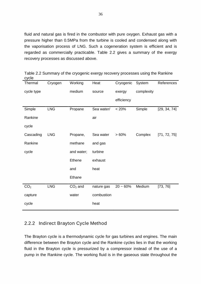
36

fluid and natural gas is fired in the combustor with pure oxygen. Exhaust gas with a

pressure higher than 0.5MPa from the turbine is cooled and condensed along with

the vaporisation process of LNG. Such a cogeneration system is efficient and is

regarded as commercially practicable. Table 2.2 gives a summary of the exergy

recovery processes as discussed above.

Table 2.2 Summary of the cryogenic exergy recovery processes using the RankinecycleThermal

cycle type

Cryogen Working

medium

Heat

source

Cryogenic

exergy

efficiency

System

complexity

References

Simple

Rankine

cycle

LNG Propane Sea water/

air

< 20% Simple [29, 34, 74]

Cascading

Rankine

cycle

LNG Propane,

methane

and water;

Ethene

and

Ethane

Sea water

and gas

turbine

exhaust

heat

> 60% Complex [71, 72, 75]

CO2

capture

cycle

LNG CO2 and

water

nature gas

combustion

heat

20 ~ 60% Medium [73, 76]

2.2.2 Indirect Brayton Cycle Method

The Brayton cycle is a thermodynamic cycle for gas turbines and engines. The main

difference between the Brayton cycle and the Rankine cycles lies in that the working

fluid in the Brayton cycle is pressurized by a compressor instead of the use of a

pump in the Rankine cycle. The working fluid is in the gaseous state throughout the

37

Brayton cycle and the heat or cold transferred to the working fluid is in the form of

sensible heat. Therefore the cryogenic energy could only be used to cool the inlet

gas of the compressor. Figure 2.13 (a) shows schematically a direct way of using the

cold energy to pre-cool the input working fluid in the gas cycle. The feasibility of the

use of the cold energy of liquefied natural gas to cool the inlet air has been analysed

by Kim and Ro [77] for gas/steam combined power plants during warm seasons. Air

cooling capacity and power augmentation for a combined cycle system are

demonstrated as a function of the ambient temperature and humidity in their

research, while the corresponding increase in power is larger than 8% on average if

the humidity is low enough for warm ambient air and water vapour in the air does not

condense.

(a) (b) (c)

Cryogenin

Cryogenin

Cryogenin

Cryogenout

Cryogenout

Cryogenout

HE HE

HE1

HE2

GGG

C

C

C1 C2

CB CB

GT GTGT

Fuel inFuel in

Heatsource

in

Heatsource

out

Air in

Air inFlue gas

out

Flue gasout

CP CP

CP

Figure 2.13 Schematic diagrams of Brayton cycles

(a) pre-cooling open cycle, (b) post-cooling open cycle, and (c) closed Brayton cycle (C -

Compressor, CB - Combustion, CP - Cryogenic Pump, G - Generator, GT - Gas Turbine, HE

- Heat Exchanger)

As a special Brayton cycle the mirror gas-turbine (MGT) method is introduced

recently to recycle the cold exergy of LNG [78]; see Figure 2.13 (b) where the cold

released from LNG is used to cool the exhaust gas from a turbine to increase the

output work of the turbine and part of the cold exergy from LNG is transformed to

decrease the compression work. This is different from the conventional way of

cooling only the inlet gas of the compressor. It is reported that between seven and

twenty percent of exhaust energy can be converted to useful work by introducing

three-stage inter-cooling, and the thermal efficiency of the turbine can be improved

by over 25% regardless the input of cryogenic exergy [76].

38

The two Brayton cycles discussed above are open cycles. Closed-loop Brayton

cycles have also been investigated; see Figure 2.13 (c) for a schematic diagram.

The closed Brayton cycles can be with or without a combustion process, and not

only the air or nitrogen, but also hydrogen and helium can be used as the working

fluids. As there is no water vapour in the closed cycle the working fluid can be cooled

to a much lower temperature hence cryogenic energy recovery efficiency could be

greatly improved. Table 2.3 gives a summary of the work on the cryogenic exergy

recovery through Brayton cycles discussed above.

Table 2.3 Summary of the cryogenic exergy recovery processes using BraytoncyclesThermal

cycle type

Cryogen Working

medium

Heat source Cryogenic

exergy

efficiency

System

complexity

Reference

Open

cycle

LNG Air Combustion

heat

< 20% Simple [77, 78]

Closed

cycle

LNG, LN2 Nitrogen Ambient air < 20% Simple [31, 71, 72,

79]

LNG Hydrogen Furnace

waste heat

20 ~ 60% Medium [80]

LH2 Helium Combustion

heat

20 ~ 60% Simple [81]

LNG Helium Combustion

heat

20 ~ 60% Simple [82, 83]

It should be noted that the cryogenic exergy efficiency depends on not only the

recovery cycle type but also the working pressure of the cryogen. At ambient

pressure a great portion of the cryogenic energy is released in the form of latent heat

at a very low temperature therefore the efficiency is not high. How ever in some

circumstances the cryogenic energy is extracted at a much higher pressure (for

example in Italian the natural gas enters the main pipelines of the transmission

39

system at a pressure rating up to more than 70 bar [82]) and then the cryogenic

energy releases in the form of sensible heat leading to a much high efficiency. This

is the reason the cryogenic exergy efficiency of the closed cycle ranges very large in

Table 2.3.

2.2.3 Combined Method

A more efficient approach to the recovery of cryogenic exergy is the combined

method, particularly by integrating a Rankine cycle or a Brayton cycle with a direct

expansion method. In such a way, part of the thermal exergy is converted to high-

pressure exergy. In a typical combined method, the cryogen is normally pumped first

to a pressure above the critical point of the working fluid before vaporisation, which is

followed by direct expansion to form a supercritical open cycle with only sensible

heat discharged. Pilot-plant scale work based on the combined method was first

established in Japan in 1970s, where closed-loop Rankine cycles were combined

with direct expansion cycles in a LNG re-gasification process [84]; see Figure 2.14 (a)

for the flow chart. The process shown in Figure 2.14 (a) uses propane as the working

fluid for the Rankine cycles. Apart from propane, ammonia-water mixtures and Freon

have also been used as the working fluids for the combined cycles [85-88]. However,

liquefaction of these fluids involves phase change processes and the cold source is

in the form of sensible heat, the cryogenic exergy could not be extracted efficiently.

40

(b)

(c) (d)

(a)

HE

HE

HE1

HE2 HE3

HE2

HE1

HE3

CP

CPCP

CP

P

P P

G

G

G

G

CD

CD

CD

ST1

EP

GT EP

GT ST GT

EP STC

C

C

Water/Airout

Water/Airin

Heatsource

out

Heatsource

in

Heatsource

in

Heatsource

out

Heatsource

in

Heatsource

out

CB

Cryogenin

Cryogenin

Cryogenin

Cryogenin

Cryogenout

Cryogenout

Cryogenout

Cryogenout

Air in

Flue gasout

Fuel in

Heatsource

in

Heatsource

out

Figure 2.14 Schematic diagrams of combined cycles

(a) direct expansion-Rankine hybrid cycle, (b) direct expansion-Brayton hybrid cycle, (c)

Rankine-Brayton hybrid cycle, and (d) direct expansion-Rankine-Brayton hybrid cycle (C -

Compressor, CB - Combustion, CD - Condenser, CP - Cryogenic Pump, EP – Cryogenic

Expander, G - Generator, GT - Gas Turbine, HE - Heat Exchanger, P - Pump, ST - Steam

Turbine)

Figure 2.14 (b) shows a schematic diagram of combining the Brayton cycle with the

direct expansion cycle, where the cooling of the working fluid occurs through a

sensible heat discharging process, leading to a high performance of the cryogenic

exergy recovery. Bisio and Tagliafico used nitrogen as the working fluid in their

studies of a combined cycle involving a two-stage compression process with inter-

cooling and showed that the system had an overall exergy efficiency of 46% [71, 72].

41

There have been reports on the cryogenic energy recovery process for both LNG

and liquefied hydrogen [89-92], where the cold energy of the low pressure cryogens

is discharged in two stages; see Figure 2.14 (c). The high grade cold is used to cool

the low pressure working fluid before compression and the low grade cold is used to

liquefy the working fluid in a Rankine cycle. Therefore this configuration can be

regarded as a combination of the Rankine and the Brayton cycles. A particular

example for this is the oxy-fuel combustion of LNG, where carbon dioxide could be

separated in the condensation process for storage. This makes these technologies

much more promising [90, 91, 93]. The combination of a closed Brayton cycle and a

Rankine cycle with direct expansion has also been investigated by Bai and Mang

and their aim was to maximise the efficiency [34]; see Figure 2.14 (d) for a schematic

diagram. In their design, the Brayton cycle with nitrogen as the working fluid is

employed to recover the high grade cold and the ammonia-water based Rankine

cycle is used to recover the low grade cold. From the thermodynamic point of view,

the combined cycle proposed by Bai and Mang [34] could also be regarded as a

cascading system. Table 2.4 gives a summary of the work on cryogenic exergy

recovery using combined cycles as discussed above.

Table 2.4 Summary of the cryogenic exergy recovery using combined cyclesThermal

cycle type

Cryogen Working

medium

Heat source Cryogenic

exergy

efficiency

System

complexity

Reference

D + R LNG Propane,

Ammoina-

water, freon

Combustion

heat, low

temperature

waste heat

20 ~ 60% Simple [34, 74, 84-

88, 94]

D + B LNG Combustion

gas,

nitrogen, air

Furnace

waste heat

> 60% Medium [71, 72, 78]

R+ B LH2, LNG CO2/water

mixture,

Combustion

heat

20 ~ 60% Complex [89-92]

42

water/air

mixture

D + R +B LNG Nitrogen

and

ammonia

water

Low level

waste heat

> 60% complex [34]

2.2.4 Further Discussion

Cryogens contain high grade thermal energy in the form of latent heat and sensible

heat (low molecular kinetic energy and low enthalpy). Such a valuable energy could

only be extracted effectively by selecting an effective thermodynamic method based

on the thermodynamic properties and external conditions e.g. heat sources etc.

Theoretically, Rankine cycle is an effective method to extract the cryogenic energy if

a working medium with a slight higher boiling point than the corresponding cryogen

can be found. In addition, the Rankine cycle uses pumps to compress the working

fluid, which consumes very small amount of work, so the overall efficiency will not be

affected much by the irreversible compression process. However the recovery of the

cold released by the working fluid after compression has to be addressed in order to

further enhance the efficiency. Although the cascading cycle can be a solution,

process optimization is needed to find a balance between the cycle efficiency and

the system complexity.

The Brayton cycle is not an effective method to directly recover the cryogenic energy

as the cooling of a gas only requires sensible heat. A big loss of cold exergy is

therefore inevitable during the heat transfer process involving high grade latent heat

although the working fluid (gas) can be cooled to a very low temperature. A more

effective way to extract the cryogenic exergy is the use of a method that combines a

direct expansion cycle and other cycles.

Direct expansion converts part of the thermal energy into the pressure energy

through pumping the cryogen to a high pressure. If one defines the pressure exergy,

)(PE , as the maximum theoretical work obtainable by bringing the fluid to

43

equilibrium with the environmental pressure through an isothermal process at

ambient temperature, then

)],(),([),(),()( aaaaaaa TPSTPSTTPHTPHPE (2.1)

H and S standing for the enthalpy and entropy respectively of the fluid are functions

of the pressure P and temperature T . The values can be obtained from a

commercial program named REFPROP. The proportion of the pressure energy in

the cryogenic exergy can then be given as:

Pal

P

WPE

WPE

)(

)( (2.2)

where )(PEl is the exergy of liquid cryogen at ambient pressure, and PW is the

pumping power which for an isentropic process can be given by:

PbalbalP TPHTPSPHW /)],()),(,([ (2.3)

where P is the pump efficiency. In the above equations the subscripts a , b and l

represent the ambient condition, boiling point and liquid phase of the fluid. The

proportion of the pressure exergy is found to increase with increasing pressure, and

the increase is very sharp at low pressures of up to ~ 10MPa. However, the increase

tends to level off at higher pressures; see Figure 2.15 for three of the cryogens

considered with the pump efficiency taken as 0.7. Considering the rapid increase in

the pumping power consumption and the requirements for the turbine inlet pressure,

the pumping pressure should be limited to a certain value which is higher than the

critical pressure. From Figure 2.15 one can also see that the optimal working

pressure for methane is about 20MPa, while these for nitrogen and hydrogen are a

slightly higher. The pressure exergy could then be extracted through a direct

expansion process. The remaining exergy exits in the form of sensible thermal cold,

which has to be recovered in a thermal cycle, in which the pressure again plays an

important role.

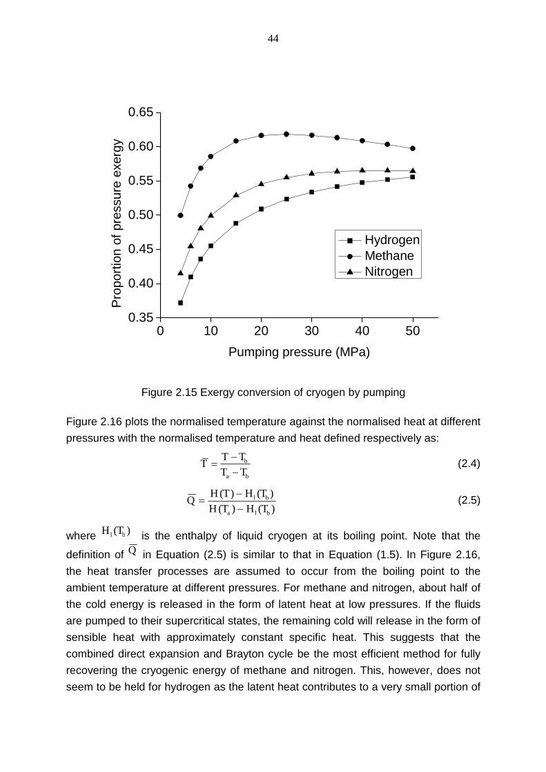
44

0 10 20 30 40 500.35

0.40

0.45

0.50

0.55

0.60

0.65P

ropo

rtio

nof

pre

ssu

ree

xerg

y

Pumping pressure (MPa)

HydrogenMethaneNitrogen

Figure 2.15 Exergy conversion of cryogen by pumping

Figure 2.16 plots the normalised temperature against the normalised heat at different

pressures with the normalised temperature and heat defined respectively as:

ba

b

TT

TTT

(2.4)

)()(

)()(

bla

bl

THTH

THTHQ

(2.5)

where )( bl TH is the enthalpy of liquid cryogen at its boiling point. Note that the

definition of Q in Equation (2.5) is similar to that in Equation (1.5). In Figure 2.16,

the heat transfer processes are assumed to occur from the boiling point to the

ambient temperature at different pressures. For methane and nitrogen, about half of

the cold energy is released in the form of latent heat at low pressures. If the fluids

are pumped to their supercritical states, the remaining cold will release in the form of

sensible heat with approximately constant specific heat. This suggests that the

combined direct expansion and Brayton cycle be the most efficient method for fully

recovering the cryogenic energy of methane and nitrogen. This, however, does not

seem to be held for hydrogen as the latent heat contributes to a very small portion of

45

the released cold. Therefore the simple Brayton cycle would be an efficient method

to recover the cryogenic energy of liquid hydrogen, if a suitable working fluid could

be found.

0.0 0.2 0.4 0.6 0.8 1.00.0

0.2

0.4

0.6

0.8

1.0

Norm

oliz

ed

he

at

Normalized temperature

Hydrogen (0.1MPa)Hydrogen (1.0MPa)Hydrogen (10MPa)Methane (0.1MPa)Methane (3.0MPa)Methane (10.0MPa)Nitrogen (0.1MPa)Nitrogen (2.0MPa)Nitrogen (10.0MPa)

Figure 2.16 Normalised heat vs. normalised temperature diagram of cryogens at lowtemperature range

It should be noted that the heat source plays a very important role in the selection of

the recovery method. If the environmental heat (seawater and air) and other low

grade heat sources are available, the Rankine cycle is more suitable whereas the

Brayton cycle is more suitable when medium and high grade heat sources are

available.

2.2.5 Summary

This section reviews the work on energy extraction process of cryogen. It covers

both the current status of technologies for cryogenic energy extraction and the

associated thermodynamic aspects. The following observations are obtained:

If a high grade heat source is available, the direct expansion - Brayton hybrid

system is the most efficient method to extract the cryogenic exergy for most

cryogens but not liquid hydrogen. This is because the latent heat of hydrogen

46

only contributes to a small part of the released cold and a simple Brayton

cycle would be suitable for the exergy recovery.

If there is only ambient and / or a low grade heat source, the combination of

direct expansion and Rankine cycle is more attractive due to its low power

consumption in the compression process.

2.3 Hydrogen and Liquid Air/Nitrogen as Energy Carriers

Besides cryogens such as liquid air/nitrogen, it is well-known that hydrogen has been

regarded as a popular carrier of renewable energy in remote locations [95-97]. Using

such a chemical energy carrier, renewable sources such as the ocean energy

generates electricity first, which is then used to electrolyze water to produce

hydrogen. Hydrogen is then transported to the end-users for transforming back to

electricity or kinetic energy by a fuel cell or other devices. This process can be split

into three sub-processes: hydrogen production for energy storage, hydrogen storage

and/or transportation and chemical energy extraction.

The ocean energy is used as an example of the use of renewable energy sources in

remote locations in this section as the world’s oceans could emerge as an important

source to provide an economically viable renewable energy source [98]. Ocean

winds blow harder and are more consistent than the wind on lands. This offsets the

greater cost of building offshore wind power facilities. Oceans tides also contribute

massive amounts of renewable energy that is gravitationally derived through the

interplay of the earth and the moon. The energy from ocean waves and tidal streams,

along with ocean-based wind energy, make the world’s oceans a source of

renewable energy that may in the next few decades be an economical alternative of

solar radiation.

Figure 2.17 illustrates schematically the use of ocean energy with hydrogen and

liquid air/nitrogen as the energy carriers. This section aims to assess and compare

the chemical energy carrier, hydrogen, with the physical energy carrier liquid

air/nitrogen in terms of the overall efficiency, including production, storage and

transportation, and energy extraction. The environmental impact, waste heat

recovery and safety issues are also considered.

47

Wind

Waves

Tides

Mechanicalenergy

Air

Electricalenergy

Water

Hydrogen Hydrogen

Water

Air/Oxygen

Cryogen

Air

Heat source

Cryogen

pre-processing Re-gasification

ENERGY EXTRACTIONSTORAGE/TRANSPORTATIONCARRIER PRODUCTION

Figure 2.17 Diagram of ocean energy utilization

2.3.1 Carrier Production

Two main technologies used to produce hydrogen are considered in this section,

reforming reaction and water splitting. The most common hydrogen production

method in commercial use today is the former, which uses hydrocarbons or other

chemical compounds such as coal and biomass as feed stocks. However, as the

renewable resources considered here (wind, tides and waves) contain only the

mechanical energy of moving masses of air or water, direct chemical path of

hydrogen production is to split water using electrical energy generated by the kinetic

energy of renewable resources. Therefore, hydrogen production using the ocean

resources can be described as follows. The kinetic energy of moving masses (air/

seawater) is extracted first by mechanical machines to form the mechanical energy

of the machines. The fraction of extractable power depends on the form of energy

and extraction processes and devices, and is limited by a theoretical value

determined by the thermodynamics. For example the upper bound of the wind

energy extraction by an ideal horizontal axis machine is 0.593 (power coefficient)

under some rather general assumptions [99]. Then the mechanical energy of the

mechanical machines is converted to electricity with a conversion efficiency of about

75~95%. Finally, the electrical energy is employed to produce hydrogen by

electrolysis. Table 2.5 summarizes the performance of electrolysis technologies,

48

along with their feed stock and efficiencies (defined as the low heating value of

hydrogen produced divided by electrical energy consumed in the electrolysis cell)

[100-105]. In the summary table, the high-temperature electrolysis efficiency is

dependent on the temperature at which the electrolyzer operates and the efficiency

of the thermal energy source. If everything is considered, the efficiency of converting

mechanical energy to chemical energy (hydrogen) is within a range of 37.5~66.5%.

Table 2.5 Efficiencies of the different electrolysis technologiesElectrolysis Technology Feed stock Efficiency Maturity

Alkaline Electrolyzer water + electricity 50 ~ 63% Commercial

PEM Electrolyzer water + electricity 55 ~ 70% Near term

Solid Oxide Electrolysis Cells water + electricity + heat 40 ~ 65% Med. Term

As mentioned before, the cryogen production is done by the air

separation/liquefaction process in which cryogenic coolers liquefy the main

components of air through the well-known Joule-Thomson effect. Although the

process is energy-intensive, the compression and refrigeration processes could be

directly powered by the mechanical work of the ocean energy. Therefore cryogen

production could be more competitive than hydrogen production in terms of the

overall efficiency and capital costs as the electricity conversion process is not

essential at the cryogen production end.

2.3.2 Carrier Storage and/or Transportation

As the energy carriers are produced at the offshore power generation facility, they

have to be stored and transported to an onshore location for distribution to the end-

users. Hydrogen could be delivered to onshore facilities through one of the three

forms: gas (compressed), liquid (liquefied), or solid (in a solid hydrogen carrier). In

the gaseous form, hydrogen can be compressed and transported to onshore in

pressurized containers. Because of its low molecular weight, hydrogen molecules

are very small and leakage can be an issue particularly at high pressures. Because

of this, the storage pressure of hydrogen is limited to ~35 MPa at present.

Liquefaction of hydrogen and its transportation in containers are an established

technology. However, the liquefaction process is energy-intensive and about

30~40% of the energy content is lost in the liquefaction process [106]. Because of its

49

added complexity and costs for both generation and transportation, the use of liquid

hydrogen is not regarded as an attractive option.

Table 2.6 shows the volumetric capacity of hydrogen under different conditions. The

energy density increases linearly with increasing storage pressure, and liquid

hydrogen has a higher value. As mentioned above, high-pressure storage of

hydrogen gas is limited by the possible leakage. This imposes potential safety issues

[107]. A promising way to replace the conventional hydrogen fuel storage methods is

to use a solid state hydrogen carrier, which refers to any substance that can store

and transport hydrogen in either a chemical or a physical state. The advantages of

using solid carriers are better safety and reliability in comparison with liquid or

compressed gas storage methods. The carrier is charged with hydrogen at the

offshore generation site and transported to onshore where hydrogen is stripped off.

The carrier needs to be taken back for recharging (two-way carrier) or decomposed

at the point of hydrogen use (one-way carrier). Examples of hydrogen carriers

include ammonia (one-way) and liquid hydrocarbons and metal hydrides (two-way).

It is reported that some of the hydrogen carriers could attain a volumetric capacity as

high as liquid hydrogen [108, 109]. However the weight of current hydride substrates

and their container is much greater than that of the stored hydrogen, so extra energy

is required during both charging and discharging processes. While considerable

effort has been made on the hydrogen carrier technology, no reports have been

found so far on the commercial use of the carriers.

Table 2.6 Volumetric capacities of the energy carrier under different conditionsEnergy Carrier Liquid

Air

Liquid

Nitrogen

Compressed Hydrogen* Liquid

Hydrogen*

Pressure (bar) 1 1 50 150 250 350 1

Volumetric capacity

(kWh/m3) 177 171 133 377 593 785 2360

* The pressure potential energy of the compressed hydrogen and the cryogenic energy of liquid

hydrogen are not considered as they are much lower than the chemical energy.

50

Compared to hydrogen, the delivery of cryogen is much easier. Once produced and

stored in insulated containers, cryogen is ready to be delivered. No extra energy

required except for the pumping power consumption which is negligible for a liquid.

As shown in Table 2.6, the volumetric energy density of cryogen is much lower than

that of liquid hydrogen but at the same order of magnitude as compressed hydrogen.

It should be noted that the volume-based energy densities of both cryogen and

compressed hydrogen gas (at practicable pressures) are significantly lower than that

of traditional fossil fuels. In addition, cryogen is continuously vaporized and lost as

boil-off gas (BOG) during storage and transportation. The amount of BOG depends

on the design, the operating conditions of cryogenic tanks and the environment

conditions. This is reported that the typical boil-off rate ranges between 0.05% and

0.15% per day for large scale storage [110, 111].

2.3.3 Energy Extraction of the Carriers

Upon delivered to end-users’ side, the energy stored in the energy carriers is

extracted. Current technologies converting the chemical energy of hydrogen to

mechanical energy or electricity energy use one of the two methods, combustion and

electrochemical conversion in e.g., a fuel cell.

For the combustion method, both hydrogen internal combustion engines and

hydrogen fuelled gas turbines have been investigated [112-114]. Because of high

burning temperatures, hydrogen internal combustion in a conventional engine

produces a very high level of nitrogen oxides which cause environmental problems.

Although a number of ways have been proposed to reduce nitrogen oxides

emissions, efficiency decrease of the engine is inevitable. This is a serious issue as

currently the low heating value (LHV) efficiency of internal combustion is only 20 ~

35%. Another approach is the use of gas turbines in hydrogen fuelled combustion

prior to which pure oxygen is generated from an air separation unit to avoid the

production of nitrogen oxides. In such a process, water/steam is often added to

reduce the turbine inlet temperature, see Figure 2.18(a). Here water is preheated by

the exhaust gas from the gas turbine. Different from the internal combustion, the

burning temperature of these cycles is limited by the turbine inlet temperature (TIT)

which is currently about 1300 °C. In these cycles the exergy loss is mainly caused by

preheating and mixing of the three inlet stream reactants in the combustor which

accounts for about 40 ~ 50% of the overall exergy loss. This, plus energy

consumption associated with oxygen production, the overall LHV efficiency of this

51

type of cycles is limited to about 50% using current technologies and may increase

to about 60% if the turbine inlet temperature is increased to ~2000 °C with future

developments in turbine and material technologies [115].

(a) (b)

Figure 2.18 Diagrams for hydrogen fuelled gas turbine cycles

A different approach to the direct combustion of hydrogen is the so-called chemical-

looping method for extracting chemical energy of hydrogen as shown in Figure

2.18(b). Such a method uses two successive reactions, metal oxide reduction with

hydrogen, and subsequent oxidation of the metal by air, yielding the metal oxide and

a high-temperature flue gas. The resulting high-temperature gas is then used to

power turbines. By adding a chemical-looping process, the exergy loss in the

combustion process decreases significantly [116, 117]. It is claimed that the LHV

efficiency of hydrogen in such a cycle could be as high as 63% [115, 118].

Another approach for enhancing hydrogen energy extraction efficiency is the use of

fuel cells, which could replace internal combustion engines and turbines as a primary

way to convert chemical energy to kinetic or electrical energy. Fuel cells work via

electrochemical principles, and hence are more efficient than heat engines. Table

2.7 [119-121] lists the technical information of three types of hydrogen fuelled fuel

cells including typical efficiencies, operating temperatures, catalysts and other

operating parameters, where the efficiency refers the cell efficiency and the system

efficiency is generally 10% lower. However, there are still a number of barriers for

the industrial take-up of the fuel cell technologies; these include requirements for

52

high purity of hydrogen, high manufacturing costs, low cell reliability and short

service life. It is reported that the cost of fuel cell technologies is about 4~5 times

more expensive than the combustion engines/turbines, while its service life 2~3

times shorter [122].

Table 2.7 Efficiency of hydrogen fuel cellsFuel cell type Operating

temperature

(°C)

Electrolyte Catalyst,

anode

Electrical

efficiency (%)

Qualified

power (kW)

Alkaline (AFC)

70 ~ 100

KOH (aqueous

solution) Ni 60 ~ 70 10 ~ 100

Proton

exchange

membrane

(PEM)

50 ~ 100

polymer

membrane Pt 50 ~ 70 0.1 ~ 500

Phosphoric

acid (PAFC) 150 ~ 220

Phosphoric acid

(immobilized

liquid)

Pt 40 ~ 55 5 ~ 10000

In contrast to hydrogen, energy extraction from cryogen is much more

straightforward which is similar to a steam engine but expansion of cryogen does not

emit pollutants such as NOX and particulate matters etc. The methods for cryogenic

energy extraction have been discussed in previous section and it has been

concluded that the exergy efficiency could achieve to 60% or even higher. The

exergy efficiency of cryogen expansion could be further enhanced if the working fluid

is superheated by waste heat or heat from other renewable sources such as solar. At

present, only high grade waste heat in gas turbine power cycles could be recovered

efficiently by heat recovery steam generator (HRSG) technology while low grade

heat is generally vented. The use of a cryogen expansion cycle can be a very

53

effective way to recover such low grade heat as the boiling point of air or nitrogen is

much lower than the ambient temperature.

2.3.4 Summary

This section assesses and compares two energy carriers, hydrogen and cryogen, as

examples for ocean energy sources exploitation. The assessment and comparison

are based on the overall efficiency including production, storage and transportation,

and energy extraction. The environmental impact, waste heat recovery and safety

issues are also touched upon. The following observations are drawn:

The production efficiencies of hydrogen and cryogen are similar at 40~65%

based on the current technologies. However, cryogen may be more

competitive than hydrogen as an energy carrier in terms of capital costs

because electricity conversion may not be absolutely necessary at the

cryogen production end.

As an energy-intensive process which consumes up to ~40% of the chemical

energy, pre-treatment is required for the storage and transportation of

hydrogen regardless of the form of the carrier being compressed gas,

liquefied hydrogen or solid hydrogen carrier. In addition, the transportation of

hydrogen carrier may be two-way if the two-way carrier is adopted. In

contrast, transportation of cryogen requires neither pre-treatment nor other

carriers but insulated containers. However it should be noted that hydrogen

has a higher volumetric energy density than cryogen regardless of storage

forms.

The energy extraction efficiency of hydrogen depends significantly on the

conversion methods. Currently, gas turbine and fuel cell methods have better

performances than conventional internal combustion engines though

significant developments are needed in order for the fuel cell technologies to

be competitive. Cryogen engines, if cold recovery technology is employed,

may have an even higher efficiency than the fuel cell technologies.

Waste heat especially low grade heat could be recovered efficiently by the

use of cryogen engines.

Although hydrogen is regarded as a clean fuel, nitrogen oxides can be

produced if air is used as an oxidant. Cryogen is much more environmentally

friendly as the processes of production (using the ocean energy) and

54

extraction are both physical involving no chemical transformation. Even the

transportation of the cryogen can be cryogen-based.

Overall, hydrogen is viable as an ocean energy carrier only if a practical method to

store and carry hydrogen is introduced and fuel cells become cheap with their

service life much improved. Before these are achieved, cryogen appears to be a

more attractive energy carrier as there are few technical difficulties to overcome.

Moreover, the overall efficiency of the use of cryogen can be greatly increased if low

grade heat is used in the process of cryogenic energy extraction. Low grade heat

can be obtained easily from either traditional energy intensive industries like steel

plants or directly from the abundant renewable solar energy. As mentioned before,

the electricity conversion efficiency of solar energy is limited, it is much easier to use

solar thermal energy in countries blessed with good sunshine (e.g., India with a

mean daily solar radiation of 5~7 kW/m2 [123]) via e.g., a cascading way. Solar

energy, along with the thermal energy storage technology using e.g., phase change

materials, has been extensively studied and used for heating, cooking and even

electricity production [124-126]. Therefore, a solar-cryogen hybrid energy storage

system appears to be a promising way for both transportation system and electricity

production. This will be explored as part of this work.

2.4 Summary of the Literature Review

A wide variety of articles focusing on the gas liquefaction technology are presented

in the literature. Cascade refrigerant cycle and MRC and their combinations are the

dominant technologies for large scale liquefaction of natural gas. The exergy

efficiency could attain up to 55% if multistage compression is adopted with inter-

cooling. However such methods are not favorable for air liquefaction in CES as they

require constant operation.

Gas liquefaction technologies based on expander cycle enables a rapid startup and

shutdown. As a consequence it is likely to be more suitable for excessive electricity

storage. The practical exergy efficiency of this technology is lower than 30%. And

some conceptual designs are being developed which have been shown to achieve a

potential exergy efficiency of 60% and higher. However both of the practical

application and theoretical modelling focus on the liquefaction of hydrogen and

55

helium and they fail to address concerns that arise from air separation and

liquefaction.

A significant amount of research work has been conducted in the cryogenic energy

extraction as well in the literature which can be categorised into indirect Rankine

cycle method, indirect Brayton cycle method and combined method. The work shows

that for most cryogens (but not liquid hydrogen) the direct expansion – Brayton

hybrid cycle is the most efficient method if a high grade heat source is available. On

the other hand if only ambient and / or a low grade heat sources are available, the

combination of direct expansion and Rankine cycle is more attractive due to its low

power consumption in the compression process.

However the studies of both gas liquefaction and cryogenic energy extraction

provide insight on the performance investigation of specific systems. Optimisations

of the system configuration are not well documented in the literature. The present

work aims to develop a systematic optimisation strategy which enables configuration

selection and parametric optimisation at the same time. This strategy is used for the

optimisation of the expander cycle based air liquefaction process in CES and other

integrated systems related to CES technology.

A comparison of hydrogen and liquid air/nitrogen as energy carrier is also studied

based on the literature in terms of production, storage and transportation, and

energy extraction. The overall performances of the two carriers are similar if no

external heat sources are available for cryogenic energy extraction. There are fewer

technical difficulties to overcome for liquid air/nitrogen than that for hydrogen. More

importantly, the exergy efficiency of cryogenic energy extraction could be

significantly improved if a heat source is used to superheat the cryogen. Therefore

liquid air/nitrogen is regarded as a more attractive energy carrier before conquering

both technical and economic barriers related to hydrogen.

56

Chapter 3 Methodologies for Modelling and Optimisation

3.1 Thermodynamic Modelling

3.1.1 Component Modelling

Thermal energy system is made up of thermodynamic cycles, either closed-loop or

open-loop. A thermodynamic cycle consists of a series of processes realised by

power transfer units and heat transfer units; see Figure 3.1. In a single phase

process the power transfer units include expanders (gas turbine, steam turbine and

liquid expander or other expansion engine) and compressors (gas compressor and

liquid pump).

Defining the isentropic efficiency of the expander as (see Figure 3.2 for an example

of steam turbine):

ieOI

rOI

EPHH

HH

,

,

(3.1)

The real power generated from the expander could be expressed as:

EPOI HHW )( ie, (3.2)

In equation (3.1) and (3.2) IH is the input enthalpy, ie,OH and r,OH are respectively

the idea output enthalpy after an isentropic expansion and the real output enthalpy,

W is the real specific power output of the expander.

I1 I2 I3 INO1 O2 O3 ON-1ONI4

HF1 HF2 HF3 HFN-1

C1 C2 C3 CN

I1 I2 I3 INO1 O2 O3 ON-1ONI4

HF1 HF2 HF3 HFN-1

C1 C2 C3 CN

Figure 3.1 Diagram of a generalized thermodynamic cycle(I – Inlet, O – Outlet, C – Power Component, HF – Heat Flux)

57

0 2 4 6 8 10

400

600

800

1000

Tem

pe

ratu

re(K

)

Entropy (kJ/kg/K)

Inlet

Outlet,isentropic

Outlet,real

Isobaric line

Figure 3.2 A Temperature-Entropy diagram showing an expansion process of asteam turbine

Practically the expansion could be regarded as an adiabatic process. The actual

output enthalpy can be calculated as:

IEPIOrO HHHH )( ie,, (3.3)

In equations (3.3) rOH , is the actual output enthalpy.

There are two types of compression named adiabatic process and isothermal

process. The compression processes without cooling could be regarded as adiabatic

compression. In adiabatic compression the isentropic efficiency is defined similarly

as the expansion process:

IrO

IieO

ACHH

HH

,

, (3.4)

In equation (3.4) AC is the isentropic efficiency of the compressor. The real power

consumption in the compression process is calculated as:

ACOI HHW /)( ie, (3.5)

Again the actual output enthalpy of the adiabatic compressor is calculated as:

58

ACOIIrO HHHH /)( ie,, (3.6)

On the other hand if ambient thermal sources such as air or water are used for

process cooling the compression is considered as an isothermal compression. The

ideal power consumption in an isothermal compression is the exergy change.

Considering the irreversibility the real power consumption is expressed as:

ICOIaOI SSTHHW /)]()[( it,it, (3.7)

And the output enthalpy of the isothermal compression is calculated as:

it,, OrO HH (3.8)

In equations (3.7) and (3.8) IS is the input entropy, it,OH and it,OS are respectively

the idea output enthalpy and entropy after an isothermal expansion, IC is the

isothermal efficiency of the compressor.

In the present study the process is regarded as adiabatic compression while the

working temperature is lower than the ambient temperature due to cooling

technology is not applicable using the ambient thermal sources. Otherwise the

isothermal model is applied to represent an ambient-temperature compression using

water/air cooling technologies. Note that the power consumption of the compressor

is negative for the convenience of the whole system design.

The throttle valve is neither a power transfer unit nor a heat transferring unit but

could be regarded as a zero-output power transfer unit 0W . As working fluid

expands through an isenthalpic process the mass fraction of fluid that is liquefied can

be calculated as:

gOlO

gOI

HH

HHx

,,

,

(3.9)

In equation (3.9) x represents the liquid fraction, lOH , and gOH , represent

respectively enthalpies of output liquid and gas. It is noted that in a throttling device

the working fluid expands through an isenthalpic process and theoretically this can

lead to either an increase (when the Joule-Thomson coefficient is negative) or a

decrease (when the Joule-Thomson coefficient is positive) in temperature; see

Figure 3.3 for an example using methane. From the figure one can see that the high-

pressure fluid can be fully liquefied if it is cooled to a sufficient low temperature prior

59

to the throttle valve. In other words, the fluid could be fully liquefied with 1x when

lOI HH , .

Figure 3.3 Isenthalpic process of methane in a Temperature-Entropy diagram

In the heat transfer unit the heat flux could be regarded as the enthalpy difference of

the inlet and outlet flows:

iOiIi HHq ,1, (3.10)

In equation (3.10) iq is the thi heat flux, 1, iIH is the thi )1( inlet enthalpy and iOH , is

the thi outlet enthalpy.

3.1.2 Thermodynamic Properties

Accurate data of thermodynamic properties are pre-requisite for a valid

thermodynamic simulation. Numerically the thermodynamic properties could be

predicted by the equations of state. One of the simplest equations of state for this

purpose is the ideal gas law, which is roughly accurate for gases at low pressures

and above moderate temperatures. However, this equation becomes increasingly

less accurate at higher pressures and/or lower temperatures, and fails to predict

condensation from a gas to a liquid. These cases occur in the current study. As a

result, a valid prediction method for the thermodynamic properties is required.

60

A number of equations of state have been developed for gases and liquids since Van

der Waals proposed his well-celebrated equation account for the real gas effects.

Examples include Redlich and Kwong equations and Peng and Robinson equations

[127]. These equations are empirical based and no one can accurately predict the

properties of all substances under all conditions. In the present study a commercial

program named REFPROP is used, which is able to provide the most accurate

predictions for pure fluids and mixtures among all methods that are currently

available.

REFPROP, developed by the US National Institute of Standards and Technology

(NIST), provides tables and plots of the thermodynamic and transport properties of

industrially important fluids and their mixtures with an emphasis on refrigerants and

hydrocarbons, especially natural gas systems. This program includes three models

to calculate the thermodynamic properties of pure fluids: equations of state (explicit

in Helmholtz energy), the modified Benedict-Webb-Rubin equation of state, and an

extended corresponding state (ECS) model. These models are implemented in a

suite of FORTRAN subroutines. Written in a structured format, they are internally

documented with extensive comments, and have been tested on a variety of

compilers. Routines are provided to calculate thermodynamic and transport

properties at a given (T,D,x) state, where T is temperature, D is density and x is

mass fraction of the liquid. Iterative routines provide saturation properties for a

specified (T,x) or (P,x) state, where P is pressure. Flash calculations describe single-

or two-phase states given a wide range of input combinations (P,h,x), (P,T,x), etc,

where h is enthalpy. The accuracy of REFPROP is obtained through the use of many

coefficients in the equations, and thus the calculation speed is slower than other

equations such as the Peng-Robinson cubic equations. The equations in the

REFPROP are generally valid over the entire vapor and liquid regions of fluid,

including the supercritical state [128].

It should be noted that the REFPROP "database" is actually a program and does not

contain any experimental information, apart from the critical and triple points of the

pure fluids. The program is friendly to self-developing users as it provides a dynamic

link library (DLL) that allows interfacing with various softwares such as EXCEL,

VISUAL BASIC & C, MATLAB, LABVIEW, etc.

61

3.2 The Pinch Technology

3.2.1 Introduction to the Pinch Technology

Most industrial processes involve transfer of heat either from one process stream to

another (interchanging) or from a utility stream to a process stream. A target in an

industrial process design is to maximize the process-to-process heat recovery and to

minimize the utility (energy) requirements. Considering the fact that most processes

involve a large number of processes and utility streams, it is a challenging task for

process engineers to answer to the following questions [129]:

Are the existing processes as energy efficient as they should be?

How can new projects be evaluated with respect to their energy

requirements?

What changes can be made to increase the energy efficiency without

incurring any cost?

What investments can be made to improve energy efficiency?

What is the most appropriate utility mix for the process?

How to put energy efficiency and other targets like reducing emissions,

increasing plant capacities, improving product qualities etc, into a coherent

strategic plan for the overall site?

In late 1978, Bodo Linnhoff, a Ph.D student from the corporate laboratory, Imperial

Chemical Industries Limited (ICI), under the supervision of Dr. John Flower,

University of Leeds, devised a new approach to describe energy flows in process

heat exchanger networks [130-133]. This was the first time to introduce the

thermodynamic principles into heat-exchanger network design, and symbolize the

establishment of a systematic methodology called Pinch Technology. Such a

technology is based upon thermodynamic principles to achieve utility savings by

better process heat integration, maximizing heat recovery and reducing the external

utility loads [134]. All the above mentioned questions and more can be answered

with full understanding of the Pinch Technology and awareness of the available tools

for applying it in a practical way.

62

Pinch Technology is used to describe and analyze the heat exchanger network

which is an important section of process design. The process design hierarchy can

be represented by an "onion diagram" as shown in Figure 3.4 [135, 136]. The design

of a process starts with the reactors (in the "core" of the onion). Once feeds,

products, recycle concentrations and flowrates are known, the separators and power

systems (the second and third layer of the onion) can be designed. The basic

process heat and material balance can then be in place, and the heat exchanger

network (the forth layer) can be designed. The remaining heating and cooling duties

are handled by the utility system (the fifth layer). The process utility system may be

regarded as a part of a centralised site-wide utility system. Using the Pinch

Technology, it is possible to identify appropriate changes in the core process

conditions that can have an impact on energy savings (onion layers one, two and

three). After the heat and material balance is established, targets for energy saving

can be set prior to the design of the heat exchanger network. The Pinch Technology

ensures these targets achievable during the network design.

Reaction

Chemical synthesis

Separation

Heat exchanger network

Site heat systems

Process development

Heat recovery

Utility heating/cooling

Site power systems

Pumps, compressors and expanders

Designprocess

Figure 3.4 The onion diagram for process synthesis

63

The practical experience has shown that the Pinch Technology can bring benefits to

a huge range of plants and processes, large and small, both within and outside

traditional process industries [135]. Improvements come not only from heat recovery

projects, but also from changing process conditions, improved operability and more

effective interfacing with utility systems, all underpinned by better process

understanding.

The Pinch Technology is now an integral part of the overall strategy for process

development and design and the optimization of existing plants, often known as

process synthesis or process integration. Furthermore, its application has broadened

a long way beyond energy aspect including Mass Pinch [137-139], Water Pinch

[140-142], Hydrogen Pinch [143, 144] and Oxygen Pinch [145, 146].

3.2.2 Principle of Pinch Technology

Pinch Technology is a simple methodology for systematically analyzing industrial

processes and surrounding utility systems with the help of the first law and second

law of thermodynamics. The first law provides the energy equation for calculating the

enthalpy changes in the streams passing through a heat exchanger. The second law

determines the direction of heat flow: in the absence of work input heat energy may

only flow in the direction of hot to cold. In practice a minimum approach temperature

(MAT) has to be maintained between the ‘hot’ process streams (which have to be

cooled to specific temperatures) and ‘cold’ process streams (which have to be

heated to specific temperatures).

The temperature-heat load diagram of a heat exchange process is plotted in Figure

3.5 which shows the opportunity for heat recovery as well as the minimum net

heating and cooling requirements. In such a diagram the point of closest approach

where available temperature driving forces between hot and cold streams are at a

minimum is defined as the process pinch point where the temperature difference

should be higher than MAT. The performance of the system is then limited by this

constraint – the pinch point – just as the strength of a chain is determined by its

weakest link. In other words if one needs a stronger chain the Pinch Technology

teaches that the most cost-effective strategy is not to replace the chain with a new

one but to increase the strength of the existing chain by selectively replacing the

64

weakest link. A simple way to increase the pinch temperature in Figure 3.5 is to shift

the heating/cooling curves along the direction of heat load.

Tem

per

atu

re

Heat Load Q

ColdTarget

Hot Target

Heat Recovery

PINCH

Figure 3.5 T-Q diagram of a heat recovery process

On the other hand, the change of pinch temperature will affect the heating and

cooling requirements of the system. The heating power and cooling power are

provided by external hot and cold utilities at unspecified temperatures sufficient to

fulfill the duty. In practice, more than one utility may be available, and there are often

price differentials between them. Therefore the selection and placement of the

appropriate utilities is a key weapon for an efficient design.

In industrial practices hot utilities supplying heat to a process may include furnaces,

steam heaters, flue gases, heat rejected from heat engines, thermal fluids or hot oil

systems, exhaust heat from refrigeration systems and heat pump condensers and

electrical heating systems. Likewise cold utilities removing heat from a process may

include cooling water systems, air coolers, steam temperature rising up and boiler

feed water heating, chilled water systems, refrigeration systems and heat pump

evaporators [135]. These utilities can be further split into constant-temperature

utilities (for example the condensing steam providing latent heat at a fixed

65

temperature), variable-temperature utilities (like the hot flue gas giving up sensible

heat over a temperature range) and a mix-type utility (for example a furnace

chamber gives out radiant heat at effectively a constant high temperature whereas

the exhaust gases can release further heat as a variable-temperature utility). Often a

wide range of hot and cold utilities can be used and some will be more convenient

and effective than others. Taking the Figure 3.5 as an example, if two constant-

temperature utilities are selected for the heat balance, two options are shown in

Figure 3.6. If the temperature of hot utility is higher than the ambient temperature, it

is obviously that the selection in option (b) is wiser as the low temperature heating

may be cheaper than high temperature heating which may need to be supplied by

dedicated devices. Likewise if the temperature of cold utility is lower than the

ambient temperature, the selection and placement of the cold utility in option (b) is

more efficient than that in option (a). This is because the biggest effect of

temperature on unit cost of utilities occurs in refrigeration systems. Below ambient

cooling needs heat pumping to the ambient temperature and the work requirement

and cost increase steeply as the required temperature falls.

Tem

per

atu

re

Heat Load Q

ColdUtility

Hot Utility

Heat Recovery

PINCH

Tem

per

atu

re

Heat Load Q

Heat Recovery

PINCH

Hot Utility

ColdUtility

(a) (b)

AmbientTemperature

AmbientTemperature

Figure 3.6 The selection and placement of utilities for energy balance

Although option (b) has a better performance than option (a), it might bring new

pinch point. As a result the selection and placement of the utilities should be done

very carefully. Furthermore the utilities themselves might be multi-stream systems

with interactive heat exchange therefore should be integrated with the whole system

to find the overall pinch. The indirect heat recovery through heat and power

conversion should also be considered in this process. Using the process heat

66

sources to preheat the inlet working fluids of expansion machines could increase the

power output while pre-cooling the inlet fluids of compression components by

process cold sources could reduce the power consumption. All of these could impact

on the heat distribution along with the temperature, which means that the

temperature-heat load profile should be modified as well. Therefore Composite

Curve and Balanced Composite Curves are introduced in Pinch Technology to deal

with these multiple stream problems.

A Composite Curve is a graphical combination of all hot or cold process streams in a

heat exchange process. While dividing all streams over any given temperature range

into two groups named heat rejection and heat sink respectively, a single composite

of all hot streams and a single composite of all cold streams can be produced in the

Temperature-heat load diagram. In Figure 3.7 (a) three hot streams with constant

heat capacity are plotted separately, where their supply and target temperatures

define a series of temperatures T1 to T5. Between T1 and T2 only stream B exists and

so the heat available in this interval is given by B∙(T1-T2). However between T2 and

T3 all three streams exist and so the heat available in this interval is (A+B+C)∙(T2-T3).

A series of values of heat can be obtained in this way and the results can be re-

plotted against the heat load as shown in Figure 3.7 (b). The resulting temperature-

heat load plot is a single curve representing all the hot streams, known as the hot

composite curve. A similar procedure gives a cold composite curve of all the cold

streams in a question.

67

(a) (b)

Tem

per

atu

re

Tem

per

atu

re

T1

T2

T3

T4

T5

T1

T2

T3

T4

T5

CP=

A

C P=B

C P=

C

Heat Load Q Heat Load Q

Figure 3.7 Formation of the hot composite curve

However this procedure is not suitable for practical simulation. As mentioned before

the thermodynamic properties in this study are obtained from REFPROP "database"

instead of a constant heat capacity model as some extreme working conditions may

be involved. This makes the above staging treatment method inadequate. More

importantly the above procedure cannot handle phase change processes which have

effectively an infinite heat capacity. An alternative to the composite curve is to

capture the exact temperature at a given heat load value. This is more applicable as

the enthalpy increases monotonously with increasing heat load. The detailed

program code used in this study for temperature capture in multiple flows can be

found in Appendix A15.

While both the hot and cold Composite Curves plotted in the same diagram include

all the utility streams at their target heat loads, the resulting curves should have no

unbalanced overshoot at either ends. Therefore the so-called Balanced Composite

Curves are particularly useful for showing the effect of multiple utilities, multiple

pinches and variable-temperature utilities on temperature driving forces in the

system and thus revealing more clearly constraints in the system design.

Based on the above discussion the stages of applying the Pinch Technology to a

practical process plant or site design are as follows [135]:

68

(1) Obtain or produce a copy of the plant flowsheet including temperatures, flow

rates, pressures and other thermal properties and produce consistent heat and

mass balances.

(2) Extract the stream data from the heat and mass balances.

(3) Select an appropriate MAT and calculate energy targets and the pinch

temperature.

(4) Examine opportunities for process change, modify the flowsheet and stream

data accordingly and recalculate the targets.

(5) Once decided whether to implement process changes and what utility levels

are used, design a heat exchanger network to recover heat within the process.

(6) Design the utility systems to supply the remaining heating and cooling

requirements, modify the heat exchanger network as necessary.

(7) Reproduce the plant flowsheet based on the modifications of utilities and heat

exchange network. Return to step (2) to study if further improvement is possible.

Although the above procedure is efficient and straightforward, the development of

appropriate designs is less evident. Based on a specific configuration, the method

here is to develop choices that are ‘close to the targets’, one then tries to eliminate

rather than to determine choices. The modification of the specific configuration

entails a great amount of manual developments that is particularly tedious for large

industrial problem [147]. Furthermore, designs based on this procedure have been

shown to be non-optimal in many cases, mainly due to its dependence on the initial

structure, although some improvements have been noted [148]. An automatic design

method therefore is desirable to overcome these drawbacks.

3.2.3 Systematic Optimisation Using Pinch Technology

Selection of an optimal configuration of a system is a difficult task. Commonly, the

best configuration is obtained by parametric comparisons of different optimal

structures, as shown in Figure 3.8. This task is highly time-consuming due to

numerous design alternatives. In addition, an inherent uncertainty exists that a better

alternative could be found [149]. For that reasons, an efficient and systematic

69

simultaneous optimisation procedure is of crucial importance for the selection of the

best design alternative.

Optimaldesign

Optimal solution 11Configuration 11

Parametricoptimization

Pinch analysis& modification

OptimalConfiguration 1

Configuration 12

Optimal solution 21Configuration 21



OptimalConfiguration 2

Configuration 22

Optimal solution N1Configuration N1



OptimalConfiguration N

Configuration N2

Figure 3.8 Common procedure of configuration optimisation

To simultaneously explore the benefits of both configuration and parameter, and to

address complex trade-offs, the best approach appears to be the establishment a

general superstructure including all possible options first, followed by optimisation to

give an optimal design [150]. The superstructure concept of heat exchanger network

has been widely used in the optimisation of energy recovery [151-155]. However

such a concept is used to deal with the arrangement of give heat flows and power

transfer components are not involved. In other words the method works with the forth

layer of the ‘onion diagram’. Some researches has also extended the application of

the superstructure to configuration selection [149, 156], but only few optional

arrangements are given in their superstructure model. The present research extends

the concept of superstructure and develops a generalized model for the systematic

optimisation of complex thermal systems. In the proposed model not only the heat

exchanger network but also the selection of power transfer components and the

interactions between power transfer component and heat flow are considered.

Different to the existing superstructure the generalized model includes all the

possible options of system configurations and therefore enables optimisation at a

systematic level.

A thermal cycle has two features. One is the alternative arrangement of power

transfer units and heat transfer units as mentioned before. The other is the stream

splitting and converging. As the stream converging does not affect the

thermodynamic parameters of the fluids when they are regarded as different streams,

only stream splitting is considered in the systematic optimisation. Despite of the

specific heat exchanger network, the generalized superstructure of a thermal cycle

70

can be illustrated in Figure 3.9, which is a tree-like structure. This superstructure

could be simplified by the upper limit of component stages, overall component

numbers or the stream numbers of each splitting. For example if the streams

numbers of each splitting is one, namely there is no stream splitting, the

superstructure is simplified to the one as given in Figure 3.1.

I1

C11

C21

C311

C31N

C4111

C411N

C41N1

C41NN

C2N

C3N1

C3NN

C4N11

C4N1N

C4NN1

C4NNN

Figure 3.9 Generalized superstructure of a thermal cycle

Parametersinput

Compressor Pump Gas turbine Throttle valve /Liquid turbine

Pinlet < Poulet ?

Dinlet < Dliquid ? Dinlet < Dliquid ?YesYes

Yes No

No No

Figure 3.10 The selection procedure of component type

71

As can be seen from Figure 3.9, a general component model is used in the

generalized superstructure which should be determined in a simulation process. In

the present work the inlet and outlet pressure and inlet temperature is given for a

specific flow and the selection procedure of the component type is shown in Figure

3.10 (in the figure ‘D’ represents density and the subscript ‘liquid’ represents the

liquid state). One can see that decision is made first on the compression or

expansion process. This is followed by the selection of the component based on the

inlet state of the working fluid.

Any process flow diagrams can be expressed as a superstructure or a combination

of superstructures. A systematic design and optimisation procedure can then be

introduced as shown in Figure 3.11. A superstructure is first established based on

the problem and specific requirements. The thermodynamic properties of the flows

are then extracted to form a stream problem which could be optimised in both

structure and parameter selections for a better performance. Pinch technology can

be used in the optimisation process leading to an updated solution. After the

optimisation the superstructure is transformed back into process flow diagram to

check the feasibility prior to the final design.

Problem Superstructure

Initialsolution

Data

Thermodynamicproperties

Updatedsolution

Streamproblem

Compositecurves & Pinch

Final designprocess

FeasibilityProcess flow

diagram

meet the

requirements

meet the

Pinch rules

Target

Yes

Yes

No

No

ProcessOptimisation

Figure 3.11 General procedures of a systematic design and optimisation

72

From the above one can see that the key to a systematic design is the optimisation

process. As this is a complex problem including both structure selection and

parameter analysis, an effective and efficient optimisation technique is required in

order to obtain the best configuration and an optimal set of parameters.

3.3 Genetic Algorithm

3.3.1 Introduction to the Optimisation Algorithms

Superstructure based optimisation processes are in general formulated as mixed-

integer non-linear programming (MINLP) models in a mathematical programming

framework. According to the layout of the superstructure which includes all process

structure variations, the MINLP problem can be expressed by an objective function

),( yxf , non-linear performance or balance equations ),( yxh and non-linear

constraints ),( yxg together with the boundary conditions [156, 157]:

),(min,

yxfZyx

subject to 0),( yxh (3.11)

0),( yxg

In such a model the objective function, the balance equations and non-linear

constraints correspond to the net power (or its transformation), the first law of

thermodynamics and the second law of thermodynamics, respectively. The

continuous variables x represent process parameters (e.g. heat exchanger duties,

stream-split fractions) and integer variables y represent discrete decisions (e.g. the

specific structure selection). Moreover, the thermodynamic properties themselves

used in the simulation are obtained by solving a set of complex equations in

REFPROP. This makes the nonlinear nature more significant.

Any application of MINLP to systematic optimisation must address two issues. The

first involves resolving the integer decisions arising from the discretization of the

problem into temperature or heat load intervals defined by the kinks in the composite

curve. The second issue concerns continuous parametric optimisation [151, 152]. As

there is in general more than one local optimum, it is often difficult to guarantee

convergence to the global optimum for MINLP formulations, where a good starting

point for a design problem is seldom available when applying many of the commonly

used programming methods. An inappropriate initial guess could lead to a solution

stuck at a local optimum.

73

A well-known technique for improving search and avoiding local optima is genetic

algorithms (GA). Such a technique is based on the mechanics of natural selections.

Motivated by the principle of evolution and heredity, GA is started with a set of

random solutions called population instead of an initial guess. Whereas classical

optimisation methods often rely on local gradient search, GA keeps track of a

population of potential solutions. Thus GA is less sensitive to arbitrary initial guesses

of the solution. The four significant differences between GA and the traditional

search and optimization methods are [158]:

GA searches a population of points in parallel, not a single point.

GA does not require derivative information or other auxiliary knowledge; only

the objective function and corresponding fitness levels influence the directions

of search.

GA uses probabilistic transition rules, not deterministic ones.

GA works on an encoding of the parameter set rather than the parameter set

itself (except in where real-valued individuals are used).

Lots of studies using GA to solve MINLP problem have been reported showing the

successful engineering applications to process synthesis in general and heat

exchanger network synthesis in particular [55, 154, 155, 159].

3.3.2 The principle of GA

The genetic algorithm (GA) was developed by John Holland and his colleague at the

University of Michigan in 1960s. It is a search heuristic that mimics the process of

natural evolution [159]. This heuristic is routinely used to generate useful solutions in

large scale optimization problems.

GA starts with a set of random solutions called population. Individual solution is

represented in encoded form called chromosome. Each chromosome comprises of

individual structures called genes. Solutions from one population are used to form a

new population. This is motivated by a hope that the new population will be better

than an old population. In order to form a new population, GA uses genetic operators

and selection process. Genetic operators are used to generate the new solutions

74

(offspring) from the current solutions (parents). Selection is the process of keeping

and deleting some solutions from both parents and offspring for the same number of

next population. Moreover, selection is the process of choosing some parents to

generate offspring as well. In the selection process, the solutions are selected

according to their values of objective function (fitness). The better fitness they have,

the more chances of being selected. This process leads to the evolution of

populations of individuals that are better suited to their environment than the

individuals that they were created from, just as in natural adaptation. The algorithms

will repeat until a termination condition is satisfied. The best solution is returned to

represent the optimum solution.

The procedure of GA has the following steps [159]:

(1) Create a randomly generated population (feasible candidate solution).

(2) Scores each chromosome in the population by computing its fitness value.

(3) Scales the raw fitness scores to convert them into a more usable range of

values.

(4) Select chromosomes called parents based on their fitness

(5) Some of the individual chromosomes in the current population that have better

fitness are chosen as elite. These elite chromosomes are passed to the next

population.

(6) Produces offspring from the parents. Offspring are produced either by making

random changes to a single parent-mutation or by combining the vector entries of

a pair of parents-crossover.

(7) Replaces the current population with the offspring to form the next generation.

(8) Checks termination conditions and stops when one of the stopping criteria is

met. Else go to step (2) to create new populations.

From above one can see that GA creates three types of offspring for the next

generation as shown in Figure 3.12:

Elite offspring are the chromosomes in the current generation with the best

fitness values. These individuals automatically survive to the next generation.

75

Crossover offspring are created by combining the vectors of a pair of parents.

At each coordinate of the offspring vector, the default crossover function

randomly selects an entry or gene at the same coordinate from one of the two

parents and assigns it to the offspring.

Mutation offspring are created by introducing random changes or mutations to

the genes of a single parent. By default, the algorithm adds a random vector

from a Gaussian distribution to the parent.

Elite offspring

Crossover offspring

Mutation offspring

Figure 3.12 Schematic diagram of the offspring generation in GA

To sum up, GA does not use any information of derivative, and because of this,

presents good chances of escaping from local solution. As a result, the application of

GA to practical problems generally gives global optimal, or, at least, solutions more

satisfactory than those obtained by other methods.

3.4 Summary of This Chapter

This chapter provides a systematic optimization strategy for thermodynamic designs

of complex thermal/power systems. Unlike the traditional optimization methods,

which treat the configuration selection and parametric optimization separately, the

new technique performs the two simultaneously by extending the concept of

superstructure. In the new model not only the heat exchanger network but also the

selection of power transfer components and the interactions between power transfer

component and heat flow are considered. As a result the new superstructure

includes all the possible options of system configurations and therefore enables

optimisation at a systematic level. In the new optimal procedure, the Pinch

76

Technology is adopted for the overall process analysis and Genetic Algorithm is

used to solve the MINLP problems formulated from the optimization. Despite of the

specific structure of the heat exchanger network, the proposed technique gives an

automatic way avoiding tedious manual work for configuration selection.

77

Chapter 4 Integration of CES System with Liquefaction

4.1 Background

Electric utilities normally classify consumers into three broad groups: domestic,

commercial and industrial. The industrial sector has long been the largest user in

western countries although its contribution decreases recently, leading to a roughly

even split with respect to two other sectors; see Figure 4.1 for the example of EU-27

[160]. On contrast, huge electricity demand in some developing countries makes the

industrial sector a major consumer of electricity due to rapid industrialization. For

example, the industrial sector in China contributes to over 70 % of the nation’s total

electricity generation since 1998 [161]. In the year of 2005 to 2007, the industrial

electricity consumption share had increased to 79.4%, 77.7% and 78.4%,

respectively [162]. As electricity generation capacity is lower than the demand,

power cuts and erratic power supply often cause disruption of industrial production.

Peak hour shortages are more severe in some developing countries, leading to huge

discrepancies in production and operations management. Power thefts and low

quality of power supply make the situation in the power sector even worse. With the

demand far outstripping the electricity generation in these countries such as India

and China, a lot of industries are now looking for alternatives.

78

1990 1992 1994 1996 1998 2000 2002 2004 20060

400

800

1200

1600

2000

2400

2800

TW

h

Year

IndustryDomesticCommerialOthers

Figure 4.1 Final electricity consumption by sector, EU-27 (the 27 member countriesof the European Union)

Comparing with the household and commercial sectors, individual industrial

consumer requires much more electricity. In the US the industrial consumers

comprise about 0.5% of total end-use consumers serviced by electric utilities but

consume about 26.7% of the total electricity [163]. Particularly, the iron and steel

making, chemical, construction material and non-ferrous metal production industries

are the most electricity intensive sub-sectors among this sector. At present Chinese

electricity consumption in the above sub-sectors accounts for 11%, 7%, 11% and 7%

of the total national electricity consumption, respectively. The proportion of heavy

industries as a whole has been on the rise from 58.9% in 1999 to 75.3% in 2003

[162]. Iron and steel making and chemical industries are good examples as shown in

Figure 4.2 [164]. India is in a similar situation: the iron and steel sector consumes

approximately one quarter of the total industrial electric consumption at present and

this ratio is projected to increase as steel production through the arc-furnace route

increases from the present share of 25%. For steel-making industries, the electricity

consumption costs about 30% of the total production costs [165].

79

1992 1994 1996 1998 2000 2002 2004 2006 200850

100

150

200

250

300

350

400

450T

Wh

Year

Iron and steel industryChemical industry

Figure 4.2 Electricity consumptions by iron and steel industry and chemical industryin China

Large industrial energy users who buy their electricity at spot rates (which tend to be

higher when demand is high) are likely to be future consumers of bulky energy

storage facilities. The use of electrical energy storage enables generation of own

electricity at times of high demand when spot rates are high and switch back to the

grid for industrial processes operation and electrical energy storage when demand

and rates fall. Large scale energy storage technologies can store some excessive

off-peak electricity and take some pressure off utility's peak energy demand, hence

earn a name ‘load levelling’.

An issue associated with most heavy industrial processes is the cogeneration of

significant amount of waste heat. Examples include hot gases from various types of

furnaces in the steel industry and kilns in the cement industry, exhaust gases of

internal combustion engines and gas turbines, hot liquids used to cool kilns or

furnaces, etc [166]. Statistical investigations indicate that low-grade waste heat

accounts for 50% or more of the total heat generated in industry [167]. The waste

heat has considerable amount of available energy. Failure to recover the waste heat

80

leads to not only undesirable energy loss but also environmental pollution issues

[168, 169].

A traditional Rankine cycle using water as the working fluid does not allow efficient

recovery of such a waste heat below 370°C as the thermal efficiency becomes

uneconomically low [167]. Organic Rankine Cycles (ORCs) have been investigated

for power production using low grade waste heat. However, a wide range of

applications has not been achieved because of concerns about economic feasibility

and safety [170].

This chapter considers a potential application of CES for large scale heavy industries,

not only for addressing their high demand of bulky energy storage, but also for

efficient recovery of the cogenerated waste heat using a cryogen as the working fluid

to increase the power output in the energy extraction process. Air liquefaction unit is

integrated in the proposed systems. Based on the cooling power generation method

in air liquefaction process, two types of system namely Linde-Hampson CES system

and Expander CES system are studied in the following. In Linde-Hampson CES

system the cooling power for air liquefaction is mainly generated by the expansion of

the compressed air, while in Expander CES system an expander cycle is used to

produce the cooling power.

4.2 Linde-Hampson CES System

Using liquid air as an energy carrier, the CES consists of three sub-processes: air

liquefaction for energy storage, liquid air storage and cryogenic energy release. A

state-of-art study shows the upper limits of both liquefaction efficiency and cryogenic

energy extraction efficiency are about 60% as discussed in Chapter 2. That suggests

that the overall efficiency of the CES be lower than 36% if the two processes are not

integrated and no waste heat is available.

Detailed analysis indicates that a big share of exergy loss in liquefaction process is

caused by the inefficient generation of high grade cold. On the other hand the exergy

efficiency of cryogenic energy extraction could only be improved if the high grade

cold could be efficiently recovered. In this study, it is proposed to integrate the two

processes through cold storage to increase the overall exergy efficiency. The

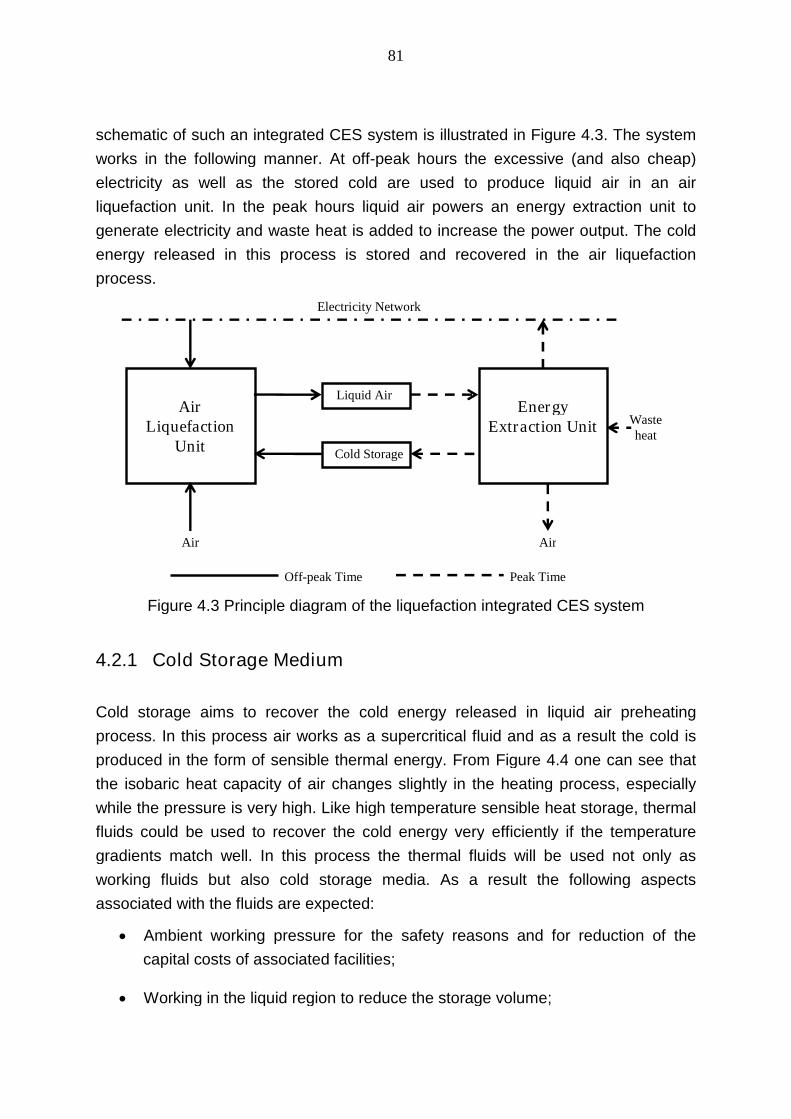
81

schematic of such an integrated CES system is illustrated in Figure 4.3. The system

works in the following manner. At off-peak hours the excessive (and also cheap)

electricity as well as the stored cold are used to produce liquid air in an air

liquefaction unit. In the peak hours liquid air powers an energy extraction unit to

generate electricity and waste heat is added to increase the power output. The cold

energy released in this process is stored and recovered in the air liquefaction

process.

AirLiquefaction

Unit

Off-peak Time

Electricity Network

Liquid Air

Cold Storage

EnergyExtraction Unit Waste

heat

AirAir

Peak Time

Figure 4.3 Principle diagram of the liquefaction integrated CES system

4.2.1 Cold Storage Medium

Cold storage aims to recover the cold energy released in liquid air preheating

process. In this process air works as a supercritical fluid and as a result the cold is

produced in the form of sensible thermal energy. From Figure 4.4 one can see that

the isobaric heat capacity of air changes slightly in the heating process, especially

while the pressure is very high. Like high temperature sensible heat storage, thermal

fluids could be used to recover the cold energy very efficiently if the temperature

gradients match well. In this process the thermal fluids will be used not only as

working fluids but also cold storage media. As a result the following aspects

associated with the fluids are expected:

Ambient working pressure for the safety reasons and for reduction of the

capital costs of associated facilities;

Working in the liquid region to reduce the storage volume;

82

Good heat capacity to reduce the storage volume;

Good stability;

Good safety performance (including flammability, toxicity etc);

High thermal conductivity to reduce the surface area of the heat exchangers;

Cheap and easy to obtain.

For the above reasons only common refrigerants are considered in this study and

their thermodynamic properties are obtained from REFPROP. The isobaric heat

capacity and thermal conductivity of the fluids are shown in Figure 4.5 and Figure 4.6

respectively and their freezing and boiling points are listed in Table 4.1 together with

the main hazards. It is found that no fluid can fully cover the working temperature

region of liquid air pre-heating process. As a result in this research the cold energy

released by the liquid air will be recovered by several stages using different

refrigerants.

60 80 100 120 140 160 180 200 220 240 260 280 300 320

0.8

1.2

1.6

2.0

2.4

2.8

3.2

3.6

4.0

4.4

Iso

bari

che

atca

pacitie

s(k

J/k

gK

)

Temperature (K)

P=7MPaP=10MPaP=15MPaP=20MPaP=35MPaP=30MPa

Figure 4.4 Isobaric heat capacities vs. Temperature diagram of air at differentpressures

83

80 100 120 140 160 180 200 220 240 260 280 300 320 340

0.8

1.0

1.2

1.4

1.6

1.8

2.0

2.2

2.4

2.6

2.8

Iso

ba

ric

hea

tca

pacitie

s(k

J/k

gK

)

Temperature (K)

PropaneR218PropyleneEthaneR12ButaneR11Methanol

Figure 4.5 Isobaric heat capacities vs. Temperature diagram of some refrigerants atambient pressure

80 100 120 140 160 180 200 220 240 260 280 300 320 340

0.06

0.08

0.10

0.12

0.14

0.16

0.18

0.20

0.22

0.24

0.26

0.28

Th

erm

alcon

ductivi

tie

s(W

/mK

)

Temperature (K)

PropaneR218PropyleneEthaneR12ButaneR11Methanol

Figure 4.6 Thermal conductivities vs. Temperature diagram of some refrigerants atambient pressure

84

Table 4.1 Freezing and boiling points and hazards of some common refrigerants

Freezing Point (K) Boiling Point (K) Hazards

Propane 85 231 Extremely flammable

R218 90 235 Non-flammable, Non-toxic

Propylene 88 225 Extremely flammable

Ethane 90 184 Highly flammable

R12 116 243 Non-flammable

Butane 136 273 Highly flammable

R11 163 297 Non-flammable

Methanol 176 338 Highly Flammable, Toxic

From Figure 4.5 and Figure 4.6 one can see the propane and ethane are prior

candidates for the recovery of high grade cold (lower temperature) as it has higher

heat capacities and thermal conductivities while comparing with other two options

R218 and Propylene. However as all these fluids become gas phases at ambient

temperature, leakage of the refrigerants may cause explosions. For these reasons

R218 is selected in this work which is non-flammable and non-toxic.

For the same reasons, R11 may be used for low grade cold recovery. It is worth to

mention that R11 may evaporate at ambient temperature (warm tank). Methanol

could be an alternative as it has a wider working temperature region. Although there

are also safety issues with the use of methanol, it is not as serious as propane

because it is in a liquid state at ambient condition.

4.2.2 System Configuration and Performance

By introducing the cold storage units, a base-case layout of the liquefaction

integrated CES system is shown in Figure 4.7. Dry air 1 and return gas 9 are mixed

and compressed to an elevated pressure 4 by a two stage compressor with inter-

cooling 2-3. After rejecting heat in the main cold box in process 4-5 the high pressure

air is cooled to the lowest temperature level, followed by an isentropic throttling

process to produce liquid air. A fraction of the product is vaporized in the cryogenic

85

tank and introduced back to the main cold box and the inter-cooler to supply part of

the cold energy. The remaining cold requirement of the main cold box is charged by

the cold storage units.

Air

Air

Heat transfer process

Cold storage tank

Turbine/Expender

Compressor

Pump

Liquid air tank

Dryer

Off-peak time

Peak time

1

19181716

1514

13

11

12

10

8

9

76

5

432

20

24

23

22

21

Figure 4.7 The flow sheet of the Linde-Hampson CES system

The liquefaction unit operates at off-peak time to store excessive electricity. At peak

time the cryogenic energy is extracted by a direct expansion cycle to reproduce

electricity. In this process, liquid air is pumped to a higher pressure level, releasing

its cold energy to the cold storage media in process 15-16 via heat exchange. It is

then superheated by waste heat before a two stage expansion with inter-heating.

The flue gas of the expander can be used to regenerate the desiccant of the air dryer.

The cold storage unit in the proposed system consists of two dual-tank

configurations in which the high temperature and low temperature fluids are stored

separately in two tanks as shown in Figure 4.7. The thermal fluids are conveyed from

high temperature tank to the low temperature tank during the energy release

processes at peak hours, and are conveyed backwards during air liquefaction

processes for cooling power supply. The use of the two thermal fluids R218 and R11

which can both transfer and store the cold energy simplifies the designs of the

system. Moreover, the operation becomes easier in this way as the mass flowrate of

the thermal fluids are easy to adjust.

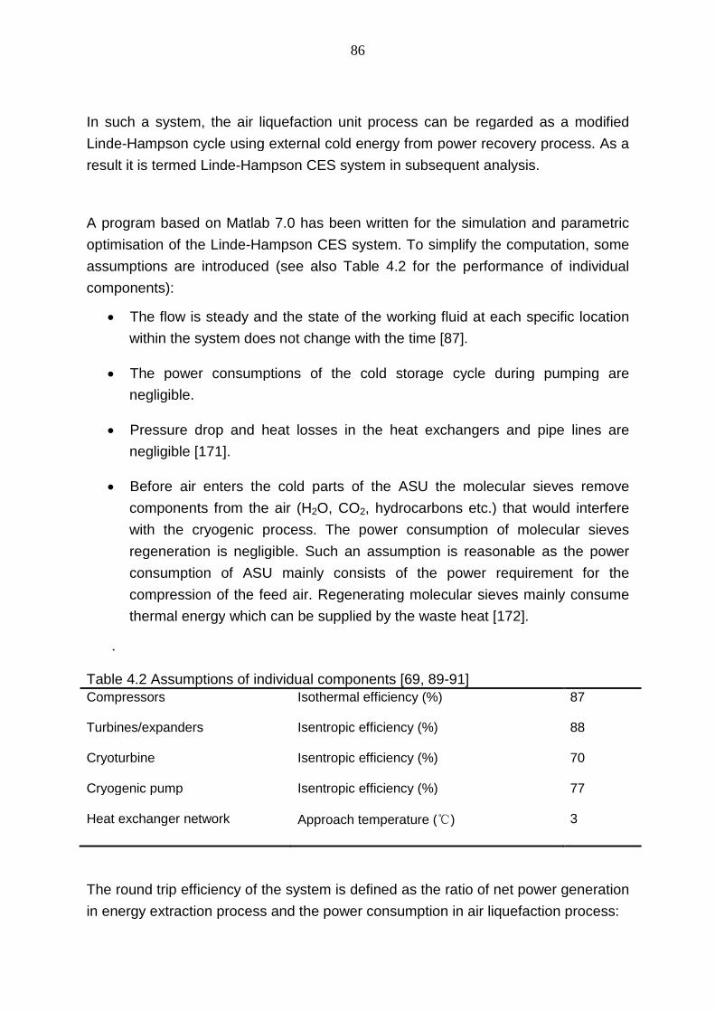
86

In such a system, the air liquefaction unit process can be regarded as a modified

Linde-Hampson cycle using external cold energy from power recovery process. As a

result it is termed Linde-Hampson CES system in subsequent analysis.

A program based on Matlab 7.0 has been written for the simulation and parametric

optimisation of the Linde-Hampson CES system. To simplify the computation, some

assumptions are introduced (see also Table 4.2 for the performance of individual

components):

The flow is steady and the state of the working fluid at each specific location

within the system does not change with the time [87].

The power consumptions of the cold storage cycle during pumping are

negligible.

Pressure drop and heat losses in the heat exchangers and pipe lines are

negligible [171].

Before air enters the cold parts of the ASU the molecular sieves remove

components from the air (H2O, CO2, hydrocarbons etc.) that would interfere

with the cryogenic process. The power consumption of molecular sieves

regeneration is negligible. Such an assumption is reasonable as the power

consumption of ASU mainly consists of the power requirement for the

compression of the feed air. Regenerating molecular sieves mainly consume

thermal energy which can be supplied by the waste heat [172].

.

Table 4.2 Assumptions of individual components [69, 89-91]Compressors Isothermal efficiency (%) 87

Turbines/expanders Isentropic efficiency (%) 88

Cryoturbine Isentropic efficiency (%) 70

Cryogenic pump Isentropic efficiency (%) 77

Heat exchanger network Approach temperature (℃) 3

The round trip efficiency of the system is defined as the ratio of net power generation

in energy extraction process and the power consumption in air liquefaction process:

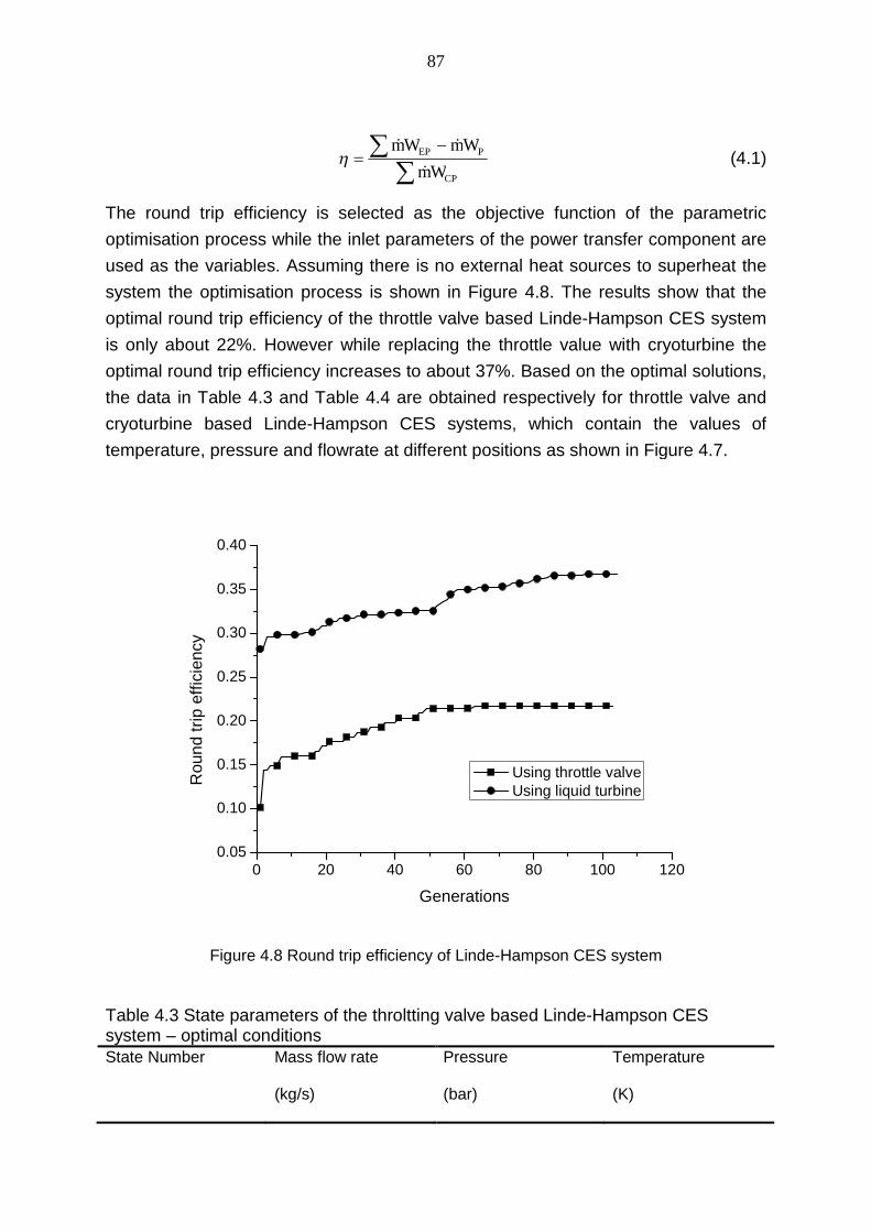
87

CP

PEP

Wm

WmWm

(4.1)

The round trip efficiency is selected as the objective function of the parametric

optimisation process while the inlet parameters of the power transfer component are

used as the variables. Assuming there is no external heat sources to superheat the

system the optimisation process is shown in Figure 4.8. The results show that the

optimal round trip efficiency of the throttle valve based Linde-Hampson CES system

is only about 22%. However while replacing the throttle value with cryoturbine the

optimal round trip efficiency increases to about 37%. Based on the optimal solutions,

the data in Table 4.3 and Table 4.4 are obtained respectively for throttle valve and

cryoturbine based Linde-Hampson CES systems, which contain the values of

temperature, pressure and flowrate at different positions as shown in Figure 4.7.

0 20 40 60 80 100 1200.05

0.10

0.15

0.20

0.25

0.30

0.35

0.40

Roun

dtr

ipeff

icie

ncy

Generations

Using throttle valveUsing liquid turbine

Figure 4.8 Round trip efficiency of Linde-Hampson CES system

Table 4.3 State parameters of the throltting valve based Linde-Hampson CESsystem – optimal conditionsState Number Mass flow rate

(kg/s)

Pressure

(bar)

Temperature

(K)

88

1 1.0 1.0 298.2

2 1.0 3.9 298.2

3 1.0 3.9 295.8

4 1.0 126.5 298.2

5 1.0 126.5 133.3

6 1.0 1.0 80.0

7 0.56 1.0 81.8

8 0.56 1.0 294.0

9 0.56 1.0 298.2

10 1.09 1.0 97.3

11 1.09 1.0 208.5

12 0.28 1.0 211.2

13 0.28 1.0 293.0

14 0.44 1.0 79.0

15 0.44 119.6 85.0

16 0.44 119.6 289.9

17 0.44 119.6 298.2

18 0.44 12.4 165.9

19 0.44 12.4 298.2

20 0.44 1.0 163.1

21 1.09 1.0 97.3

22 1.09 1.0 208.5

23 0.28 1.0 211.2

24 0.28 1.0 293.0

89

Table 4.4 State parameters of the cryoturbine based Linde-Hampson CES system –optimal conditionsState Number Mass flow rate

(kg/s)

Pressure

(bar)

Temperature

(K)

1 1.0 1.0 298.2

2 1.0 4.0 298.2

3 1.0 4.0 291.0

4 1.0 137.2 298.2

5 1.0 137.2 112.2

6 1.0 1.0 80.0

7 0.26 1.0 81.8

8 0.26 1.0 270.8

9 0.26 1.0 298.2

10 1.73 1.0 94.1

11 1.73 1.0 212.0

12 0.50 1.0 214.2

13 0.50 1.0 292.5

14 0.74 1.0 79.0

15 0.74 112.3 84.7

16 0.74 112.3 289.2

17 0.74 112.3 298.2

18 0.74 12.2 168.3

19 0.74 12.2 298.2

20 0.74 1.0 163.5

21 1.73 1.0 94.1

22 1.73 1.0 212.0

23 0.50 1.0 214.2

90

24 0.50 1.0 292.5

The data illustrate that supercritical liquefaction processes are required for a better

overall performance of the Linde-Hampson CES systems. The topping liquefied

pressures P5 are very high for both of the systems, 127 bar and 137 bar, respectively,

which are very close to the optimal topping pressure of Linde-Hampson liquefaction

process [173]. In the decompression process 5-6 such a high pressure is released to

the ambient value. As working fluid expands through an isenthalpic process in a

throttle valve, a great part of energy is lost. This part of energy transfers into the form

of heat and heats up the output products. On the other hand, part of the exergy could

be transferred to power while using cryoturbine. This not only decreases the overall

power consumption in liquefaction process but increase the output cold energy. As

seen from the mass flowrate ratios in Table 4.3 and Table 4.4 about 74% of the feed

air is liquefied in the cryoturbine based system comparing with only about 44% in the

throttle valve based system.

The other reason that cryoturbine increases the round trip efficiency is that a more

efficient heat exchange process is achieved than the throttle valve based system.

Most of the cold energy in cold box is supplied by the returning gas 7-8 with a very

low bottoming temperature of about 82K. Therefore the lower the feed gas 4-5 is

cooled to, the higher efficiency the heat exchange process has. The above data

shows that the feed air of the cryoturbine based system is cooled to about 112K

while that of the throttle valve system is about 133K. As a result the cryoturbine

should lead to a more effective heat exchange process than the throttle valve. This

effectiveness of the heat exchange process could be identified by a dimensionless

number named Effective Heat Transfer Factor.

4.2.3 Effective Heat Transfer Factor

No matter how complex a heat exchanger network is, the process can be plotted a

temperature against heat load diagram called Balanced Composite Curves; see

Figure 4.9. In the figure HT and CT are the temperature of hot fluid and cold fluid,respectively, and piT is the pinch point temperature difference. In a reversibly

infinitesimal heat transfer process the cold fluid attains a heat load of Q ( 0Q ).

As a result the exergy change of the cold fluid could be calculated as:

91

C

a

C

aCCT

TQ

T

QTdHdE 1 (4.2)

At the same time, as the hot fluid release a heat load of Q , the exergy change of

the hot fluid is expressed as:

H

a

H

aHHT

TQ

T

QTdHdE 1 (4.3)

As all the heat transfer processes produce entropy (consume exergy, 0 HC dEdE ),

the flow holds a high exergy change is regarded as exergy rejection. As a result ifthe hot fluid holds a higher exergy change ( HC dEdE ), the idea heat transfer

process can be regarded between the hot fluid and a third fluid with a temperature

piT lower than the hot fluid. On the other hand, if the cold fluid holds a higher

exergy change ( HC dEdE ), the idea heat transfer process can be regarded

between the cold fluid and a third fluid with a temperature piT higher than the cold

fluid.

Therefore the third fluid temperatures HT ' and CT ' are defined as:

aCH

piCH

aCH

CpiH

CH

TTTTTT

TTTTTT

TT211

][

211][

]''[ (4.4)

Based on the definition of third fluid, a dimensionless number named Effective Heat

Transfer Factor (EHTF) is defined in equation (4.5) to examine how effective the

process is.

2

1

2

1

11

'

111

'

1

Q

QHC

Q

QCCHH

dQTT

dQTTTT

EHTF (4.5)

In equation (4.5) 1Q and 2Q are the initial and terminated heat load values of the heat

transfer process and HT , CT , HT ' and CT ' are all the functions of heat load Q .

92

T

Q

dQ

1Q Q

)(QTH

dQQ 2Q

)(QTC

pinchT

)(' QT H

ambientT

T

Q

dQ

1Q Q

)(QTH

dQQ 2Q

)(QTC

pinchT

)(' QT H

ambientT

Figure 4.9 Balanced composite curves of heat transfer processes

EHTF ranges between 0 and 1, representing exergy loss ratio of idea heat transfer

process and actual heat transfer process. The idea heat transfer process cannot be

achieved in a practical heat exchanger network, especially where phase-change

occurs. Therefore EHTF is a parameter that indicates how close a real process

approaches to an idea heat transfer process.

Figure 4.10 shows how the EHTF value changes. It can be seen that the

dependence roughly agrees with the dependence of the round trip efficiency. One of

the important reasons for the increased round trip efficiency is due to a more efficient

heat transfer process achieved through optimisation. Note that, for the cryoturbine,

after 60 generations of optimisation, the EHTF valve still increases (Figure 4.10).

However the round trip efficiency is unchanged (Figure 4.8). This reveals the

arrangement of power transfer components could be another important factor

affecting the overall performance of the system.

93

0 20 40 60 80 100 1200.10

0.12

0.14

0.16

0.18

0.20

0.22

0.24

0.26

0.28

0.30E

HT

Fva

lue

Generations

Using throttle valveUsing cryoturbine

Figure 4.10 Corresponding EHTF values versus number of generations

Figure 4.10 also indicates that the optimal EHTF values are about 0.14 and 0.28

respectively for the throttle valve and cryoturbine based Linde-Hampson CES

systems. This implies the exergy loss of the throttle valve system in the main cold

box is as about twice as that of the cryoturbine based system. As both of the values

are much lower than 1.0, a further decrease in the exergy loss in the heat exchange

processes is still possible. This is demonstrated in next section.

4.2.4 Effect of Individual Component Performance

The influence of individual component performance on the round trip efficiency is

investigated. These include waste heat temperature, efficiencies of compressors,

turbines, pumps, cryoturbine and stages of turbines. Figure 4.11 shows the effect of

waste heat temperature while other parameters are kept constant. The round trip

efficiencies increase linearly and significantly with increasing waste heat temperature.

At a waste heat temperature of 600K which is uneconomical for power generation

using a traditional steam turbine system, the round trip efficiency reaches a value of

94

about 0.48 and 0.82 respectively for the throttle valve and cryoturbine. Therefore the

availability of waste heat is a key to the practical uptake of the CES systems.

300 400 500 600 700 800

0.2

0.4

0.6

0.8

1.0

1.2

Round

trip

eff

icie

ncy

Waste heat temperature (K)


Figure 4.11 Effect of waste heat temperature on the round trip efficiency

The influence of compressor and turbine efficiencies on the round trip efficiency are

shown in Figure 4.12 and Figure 4.13 respectively. One can observe that the

performance of compressors exerts a similar effect on the round trip efficiency as

that of turbines. Quantitatively the round trip efficiencies increase by about 1% and

2% respectively for the throttle valve and cryoturbine based Linde-Hampson CES

systems for every 4% increase in the compressor and turbine efficiencies. This

suggests that compressors and turbines be the key components that affect the

overall performance of the system. On contrast, the influences of cryogenic pumps

are negligible as shown in Figure 4.14.

95

0.75 0.78 0.81 0.84 0.87 0.90 0.930.18

0.21

0.24

0.27

0.30

0.33

0.36

0.39R

ou

nd

trip

effic

ien

cy

Isothermal efficiency of compressors


Figure 4.12 Effect of compressor efficiency on the round trip efficiency

0.75 0.78 0.81 0.84 0.87 0.90 0.93 0.96

0.20

0.25

0.30

0.35

0.40

Ro

un

dtr

ipeffic

ien

cy

Turbine efficiency


Figure 4.13 Effect of turbine efficiency on the round trip efficiency

96

0.70 0.75 0.80 0.85 0.90 0.950.20

0.24

0.28

0.32

0.36

0.40R

ou

nd

trip

eff

icie

ncy

Pump efficiency


Figure 4.14 Effect of cryogenic pump efficiency on the round trip efficiency

As a baseline study, it is assumed liquid air expands in a two-stage turbine in the

cryogenic energy extraction process. As the topping pressure P15 is very high

(>100bar), more stages might needed with inter-heating to increase the output power

(refer to Figure 4.7). Figure 4.15 shows the effects of number of stages of the turbine

in energy release process. The round trip efficiency increases with increasing stages

of expansion particularly at small stage numbers. One can also see that to attain a

good overall performance at least a four stage expansion process should be used. It

is worth to mention that a four stage turbine is currently used in a demonstration

plant by Highview Power Storage Ltd.

97

2 3 4 5 60.20

0.25

0.30

0.35

0.40

0.45

0.50R

ound

trip

eff

icie

ncy

Stages of turbine


Figure 4.15 Effect of turbine stages on the round trip efficiency

The influence of the cryoturbine performance is also examined and the results are

shown in Figure 4.16. An increase of the cryoturbine efficiency gives a great

increase in the round trip efficiency while the cryoturbine efficiency is lower than 0.75,

beyond which, the increase tends to level off.

98

0.60 0.65 0.70 0.75 0.80 0.85 0.90

0.32

0.34

0.36

0.38

0.40

Rou

nd

trip

eff

icie

ncy

Cryoturbine efficiency

Figure 4.16 Effect of cryoturbine efficiency on the round trip efficiency

4.3 Expander CES System

4.3.1 Expander Cycle

As no moving parts at the cold end Linde-Hampson CES system has a very simple

configuration. However there are two main drawbacks restricting its applications:

First is the low round trip efficiency, especially for the throttle valve based system

which has an optimal efficiency of only about 22% if there is no waste heat. Such a

low efficiency is not competitive with other energy storage technologies, even waste

heat is available.

Secondly, even such a low efficiency is only achievable with a very high liquefied

pressure. The optimal results in the previous section show the topping liquefied

pressures are 127 bar and 137 bar respectively for the two systems, leading an ultra-

supercritical process for the working air. Such a high pressure is required not only to

supply sufficient cold energy but also to attain a better match between the heat sink

and heat source. As will be discussed in the following section on the economic

99

analysis, operating the liquefaction unit at such a high pressure will dramatically

increase the capital cost of the system, especially the compressors.

Similarly, for large scale liquefaction, an effective way to overcome the above

challenges is to add a refrigerant cycle. The refrigerant cycle can supply cold energy

or transfer low grade cold energy into high grade cold energy. In this way a better

match can be obtained between the heat sink and heat source and the topping

liquefied pressure can be reduced by decreasing the cold load requirement of the

feed air. As reviewed in Chapter 2 there are three types of refrigerant cycles, namely

Cascade Refrigerant Cycle, Mixed Refrigerant Cycle and Expander Cycle. Expander

cycles are suitable for energy storage systems due to possible rapid startup and

shutdown operation. In this work the Expander Cycle is added to the Linde-Hampson

CES system to give the so called Expander CES system; see Figure 4.17.

Figure 4.17 The flow sheet of the expander CES system

In the expander cycle, the cold energy is produced by working fluid expansion. Three

working fluids, nitrogen, helium and hydrogen are often used for the expander cycles.

However, hydrogen is excluded for the safety reasons in the proposed Expander

CES system. Figure 4.18 shows a comparison of the isentropic expansion properties

between nitrogen and helium. Assuming the compressed gases are at ambient

temperature, it is illustrated that the required pressure ratio of helium is much lower

100

than that of nitrogen if they are used to generate the cold energy at the same target

temperature. The difference becomes more dramatic when the target temperature

gets lower. Therefore, the use of helium as the working fluid can lead to a much

lower topping pressure than that of nitrogen and hence a reduced capital cost.

300 250 200 150 100

0

10

20

30

40

50

Pre

ssure

ratio

Target temperature (K)

NitrogenHelium

Figure 4.18 The isentropic expansion properties of nitrogen and helium

4.3.2 Optimisation Strategy

Compared with the Linda-Hampson CES systems, the expander CES system has a

far more complicated configuration. As the expander cycle aims to generate effective

cold energy or to transfer the low grade heat to the high grade heat, a highly efficient

heat exchanger network is crucial to the overall performance of the system.

Therefore in the optimisation process the system is divided into four thermal flows as

shown in Figure 4.19 for a better approach of the heat exchanger network where air

liquefaction is considered:

(1) Air expansion flow: The liquid air is pumped to a high elevated pressure and

super-heated, followed by a two-stage expansion process in turbines/expanders

with inter-heating. The output gas exchanges the heat to about ambient

temperature and is then sent to dryers to regenerate the desiccant.

(2) Cold storage flow: Similarly to the cold storage in the Linda-Hampson CES

system the cold storage aims to store the cold energy released from the air

101

expansion flow and use the stored energy to supply the cold in the air liquefaction

process. To examine the performance enhancement of the cold storage, three

flows are considered. One uses R218 and the other two use methanol as the

storage medium.

(3) Air liquefaction flow: This flow is similar to that used in the Linda-Hampson

CES system. Dry air and return air are mixed and compressed to the elevated

pressure by a two stage compressor with inter-cooling. After rejecting heat the

high pressure air is cooled to a low temperature level, followed by an isentropic

throttling process to produce liquid air. A fraction of the product is vaporized in the

cryogenic tank and introduced back to supply part of the cold energy.

(4) Refrigerant flow: A four stage refrigerant cycle is considered to supply external

cold for air liquefaction. At each outlet of the power transfer component the heat

flow may be split into two flows. By introducing the stream splitting more system

configuration could be formed and only the one has the best performance will be

selected for the optimisation.

Feed-in Airfrom dryer

Liquid airTo dryer

(b) Cold storage flow


Cryogenic tank

Turbine/Expender

Compressor

Cryogenic pump

Liquid air

Throttling valve

Power transfercomponent

(a) Air expansion flow

(c) Air liquefaction flow

(d) Refrigerant flow

3

Figure 4.19 Sub-flows of the expander CES system

One can see that the four flows are all made up of a series of power transfer

components and heat transfer processes placed alternatively. Given the inlet

parameters (including flow rate, temperature and pressure), some outlet parameters

(e.g. outlet pressure) and configuration control parameter (whether split or not) the

system configuration could be identified and other state parameters as well as the

102

heat loads and power could be calculated. Therefore the global design method

mentioned in Chapter 3 can be used for a systematic optimisation.

4.3.3 Results and Discussion

To simplify the simulation the system are divided into two sub-systems. They are

described and discussed in the following:

The first is an energy release unit made of flow (a) and flow (b) in Figure 4.19 with

the outputs of power and cold energy stored in the cold medium. Exergy efficiency is

set as the objective function which is defined as the ratio of output exergy and input

exergy. Figure 4.20 shows the exergy efficiency and the EHTF value as a function of

the optimisation process. It is seen that an exergy efficiency as high as about 85%

could be achieved. This is because the exergy loss in the heat exchange process

decreases with increasing EHTF value as a result of systematic optimisation. The

EHTF value corresponding to the 85% exergy efficiency is about 47%. Figure 4.21

compares the temperature distributions before and after the optimisation. It reveals

that the optimisation enables a smaller temperature difference.

0 20 40 60 80 100 120 140 1600.2

0.3

0.4

0.5

0.6

0.7

0.8

0.9

1.0

Generations

Exergy efficiencyEHTF value

Figure 4.20 Changes of the exergy efficiency and EHTF value of the energy releaseunit during process optimisation

103

0 0.1 0.2 0.3 0.4 0.5 0.6 0.750

100

150

200

250

300

Heat load (MW)

Te

mp

era

ture

(K)

Initial composite curves

Hot composite curve

Cold composite curve

0 0.1 0.2 0.3 0.4 0.5 0.6 0.750

100

150

200

250

300

Heat load (MW)

Te

mp

era

ture

(K)

Optimised composite curves

Hot composite curve


Figure 4.21 A comparison between the composite curves before and afteroptimisation

The second unit is the air liquefaction system made of flow (b), flow (c) and flow (d)

in Figure 4.19. Such a unit consumes off-peak electricity and stores the cold energy

to produce liquid air. The round trip efficiency is selected as the objective function for

the optimisation and the output power and cold energy data are supplied from the

energy release unit. Figure 4.22 shows the round trip efficiency trend during

optimisation. Compared with the Linda-Hampson CES system, the expander CES

system has a much higher efficiency, about 40% for the throttle valve based system

and about 46% for the cryoturbine based system. Figure 4.23 shows the

corresponding EHTF values which are about 30% and 34% for the throttle valve and

cryoturbine systems, respectively. These values are much higher than those of the

corresponding Linda-Hampson CES systems, leading to a significant improvement of

the overall performance.

104

0 20 40 60 80 100 120 140

0.24

0.28

0.32

0.36

0.40

0.44R

ound

trip

eff

icie

ncy

Generations


Figure 4.22 Round trip efficiency of expander CES system

0 20 40 60 80 100 120 1400.12

0.16

0.20

0.24

0.28

0.32

0.36

EH

TF

valu

e

Generations


Figure 4.23 EHTF values of expander CES system

From the above simulation results, the following conclusions can be drawn:

Liquefaction unit is the key part of the CES system as the energy release unit

has a very simple configuration and a very high efficiency. Further

105

improvement on the performance of the liquefaction unit is possible as the

EHTF values are still very low.

Cryoturbine is a very important component of the CES system. Using

cryoturbine to replace throttle valve could bring at least an improvement of

about 6% on the round trip efficiency.

The availability of waste heat or heat from renewable energy sources plays a

crucial role to the application of the CES system. Without the use of waste

heat, the best optimised CES system only has a round trip efficiency of about

45%. This is less competitive with other energy storage technologies. The

round trip efficiency increases linearly with increasing waste heat temperature.

At a waste heat of above 300°C, the round trip efficiency is nearly doubled to

about 90%, making the technology highly competitive.

4.4 Economic Analysis

As the proposed technology is novel, it is necessary to estimate the capital cost

associated with the system. Detailed expressions for estimating the costs are

presented in Appendix B, which are widely used [174-177]. Note that these

expressions also take into account the cost of installation, electrical equipment,

control system, piping and local assembly.

A CES system with the net peak power of 60 MW is used as a case study for the

economic analyses. Such a scale is typical for the power requirement of heavy

industries. Further assumptions for the calculations include:

The CES system is for load levelling with air liquefaction unit to store

excessive electricity and energy release unit to generate peak load. Both the

energy release unit and air liquefaction unit can start up and shut down

instantaneously.

Waste heat is available in the heavy industries, which is sufficient to super-

heat the energy release unit of the CES system and the waste heat is

considered to be a free heat source.

The CES system operates at an optimal performance based on the

optimisation results presented in Section 4.2 and Section 4.3.

106

Other baseline assumptions for the simulation are listed in Table 4.5. In the table,

represents the operation period ratio defined as:

pk

ASU

O

O (4.6)

Where ASUO and pkO correspond the operation hours of air liquefaction unit and

energy release unit, respectively. is the maintenance factor; in is the interest rate;

ri is the rate of inflation; CP is the construction period; k is the amortizationperiod ; opkCE is the off-peak electricity price ; h is the heat transfer coefficient of the

heat exchangers; whT is the waste heat temperature.

Table 4.5 Baseline parameters for the economic analysis of the CES system 1.06

pkO (hours) 4

in (%) 6.00 2

ri (%) 5.00opkCE (US$/kWh) 0.045

CP (years) 1 h (W/(m2K)) 300.0

k (years) 30whT (K) 600

Two parameters are considered based on the above assumptions. The first is the

capital cost of the CES system, which can be expressed as [176]:

CES

CESCES

W

IC (4.7)

Where CESI is the total cost for components purchasing of the CES system and CESW

is the output power of the energy release unit.

The second is the peak electricity production cost of the CES system given by [176]:

pk

CESASUopk

CES

CESO

WfIwCE

WCE

365

1 (4.8)

Figure 4.24 shows the main component purchase costs of four optimised cases of

the CES system. One can see that turbines and compressors take the major share

of the costs. Due to high topping pressure and large mass flowrate, the cost of

compressors in the throttle valve based Linde-Hampson CES system is very high.

Replacing the throttle valve with cryoturbine, the cost of compressors is reduced by

over half as the flowrate of the input mass is reduced. In the expander CES systems

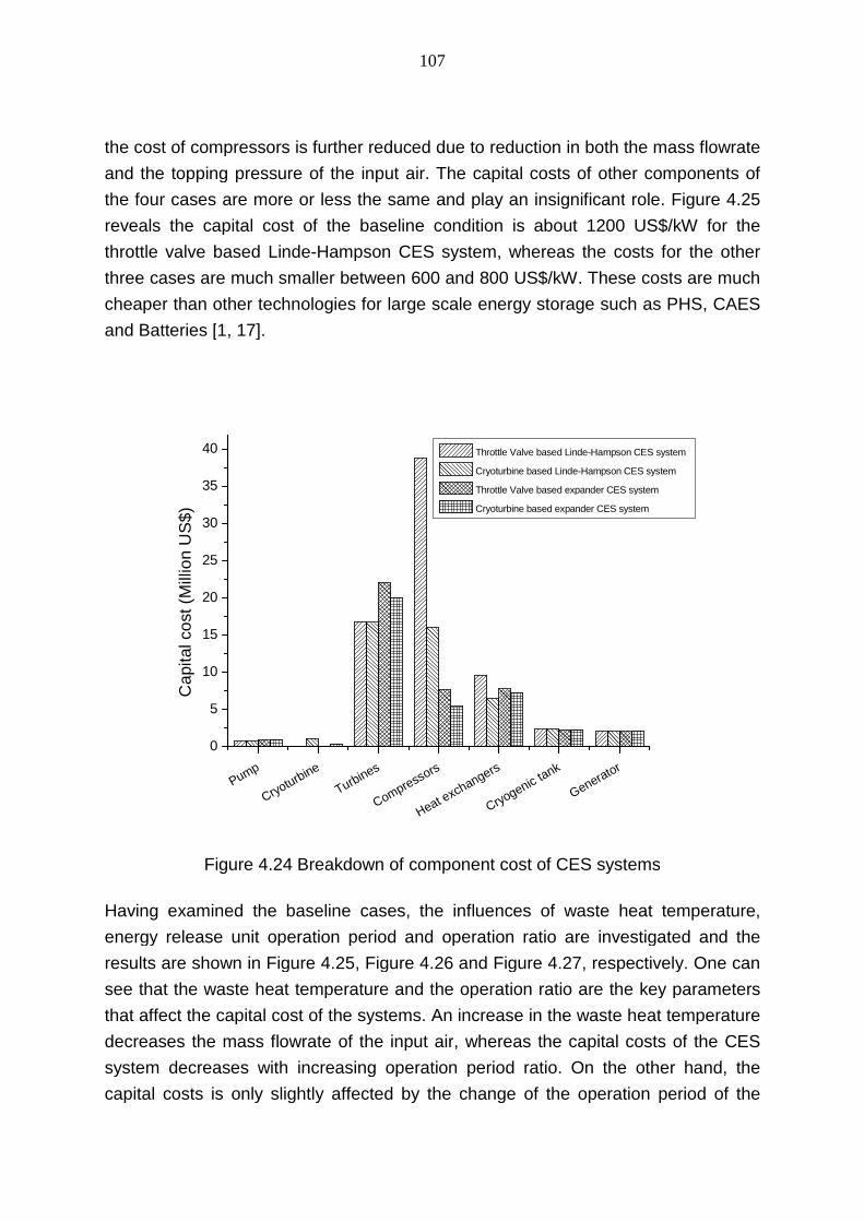
107

the cost of compressors is further reduced due to reduction in both the mass flowrate

and the topping pressure of the input air. The capital costs of other components of

the four cases are more or less the same and play an insignificant role. Figure 4.25

reveals the capital cost of the baseline condition is about 1200 US$/kW for the

throttle valve based Linde-Hampson CES system, whereas the costs for the other

three cases are much smaller between 600 and 800 US$/kW. These costs are much

cheaper than other technologies for large scale energy storage such as PHS, CAES

and Batteries [1, 17].

Pump

Cryoturbine

Turbines

Compressors

Heat exchangers

Cryogenictank

Generator

0

5

10

15

20

25

30

35

40

Capitalco

st

(Mill

ion

US

$)

Throttle Valve based Linde-Hampson CES system

Cryoturbine based Linde-Hampson CES system

Throttle Valve based expander CES system

Cryoturbine based expander CES system

Figure 4.24 Breakdown of component cost of CES systems

Having examined the baseline cases, the influences of waste heat temperature,

energy release unit operation period and operation ratio are investigated and the

results are shown in Figure 4.25, Figure 4.26 and Figure 4.27, respectively. One can

see that the waste heat temperature and the operation ratio are the key parameters

that affect the capital cost of the systems. An increase in the waste heat temperature

decreases the mass flowrate of the input air, whereas the capital costs of the CES

system decreases with increasing operation period ratio. On the other hand, the

capital costs is only slightly affected by the change of the operation period of the

108

energy release unit because this change only affect the size of the cryogenic tank for

liquid air storage. The above three figures also show that the capital cost of the

cryoturbine based system is much cheaper than the throttle valve based system,

especially for the Linde-Hampson CES system. This is because the efficiency of

throttle based system is much lower. As a result in order to give the same power

output larger scale components are required which leads higher capital costs.

400 500 600 700 800 900

600

800

1000

1200

1400

1600

Ca

pita

lco

st(U

S$/k

W)


Throttle valve based Linde-Hampson CES system


Throttle valve based expander CES system


Figure 4.25 Effect of waste heat temperature on capital cost of CES systems

109

2 3 4 5 6600

700

800

900

1000

1100

1200

Cap

ita

lcost

(US

$/k

W)

Operation period of energy release unit (hours per day)





Figure 4.26 Effect of operation period of energy release unit on capital cost of CESsystems

1.0 1.5 2.0 2.5 3.0

600

800

1000

1200

1400

1600

1800

Operation period ratio of the CES systems





Capitalcost

(US

$/k

W)

Figure 4.27 Effect of operation period ratio on capital cost of CES systems

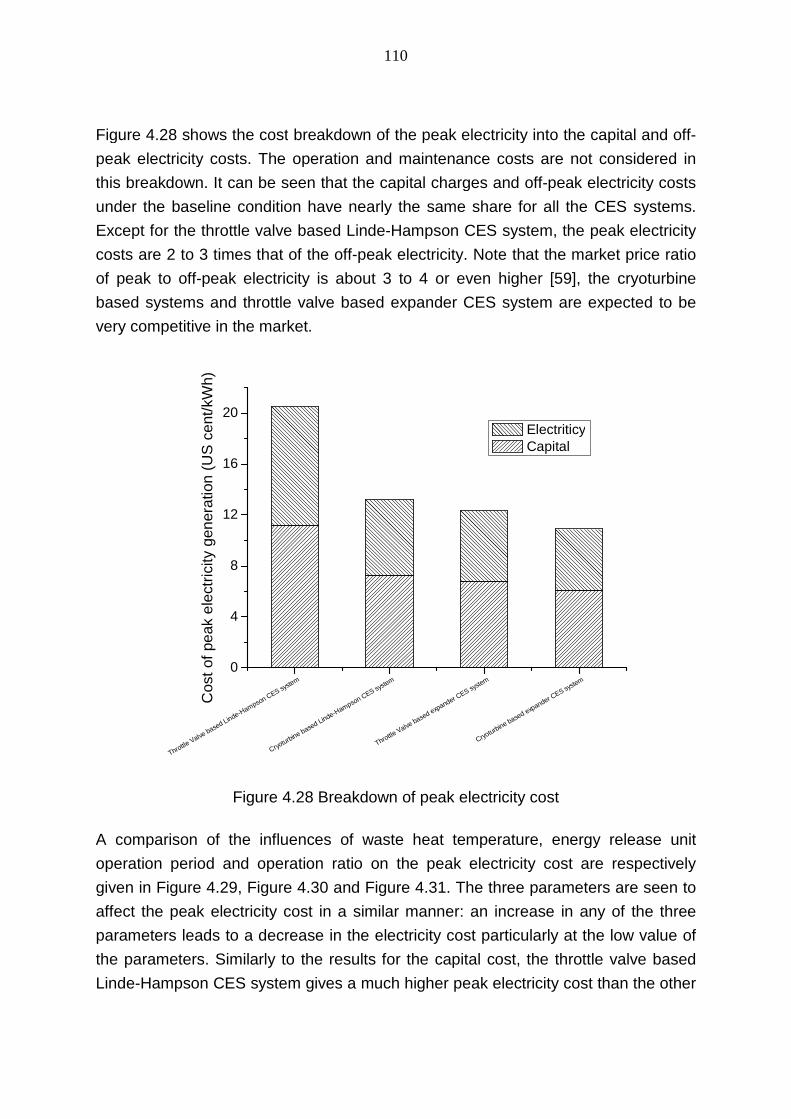
110

Figure 4.28 shows the cost breakdown of the peak electricity into the capital and off-

peak electricity costs. The operation and maintenance costs are not considered in

this breakdown. It can be seen that the capital charges and off-peak electricity costs

under the baseline condition have nearly the same share for all the CES systems.

Except for the throttle valve based Linde-Hampson CES system, the peak electricity

costs are 2 to 3 times that of the off-peak electricity. Note that the market price ratio

of peak to off-peak electricity is about 3 to 4 or even higher [59], the cryoturbine

based systems and throttle valve based expander CES system are expected to be

very competitive in the market.

ThrottleValve

based Linde-Hampson CES system

Cryoturbine based Linde-H

ampson CES system

ThrottleValve

based expander CES system


0

4

8

12

16

20

Cost

of

pe

ak

ele

ctr

icity

gen

era

tion

(US

ce

nt/

kW

h)

ElectriticyCapital

Figure 4.28 Breakdown of peak electricity cost

A comparison of the influences of waste heat temperature, energy release unit

operation period and operation ratio on the peak electricity cost are respectively

given in Figure 4.29, Figure 4.30 and Figure 4.31. The three parameters are seen to

affect the peak electricity cost in a similar manner: an increase in any of the three

parameters leads to a decrease in the electricity cost particularly at the low value of

the parameters. Similarly to the results for the capital cost, the throttle valve based

Linde-Hampson CES system gives a much higher peak electricity cost than the other

111

three systems and the cryoturbine based expander CES system has the lowest peak

electricity generation cost.

400 500 600 700 800 900

8

12

16

20

24

28

32

Cost

of

peak

ele

ctr

icity

ge

nera

tion

(US

cent/

kW

h)






Figure 4.29 Effect of waste heat temperature on peak electricity cost

112

2 3 4 5 68

12

16

20

24

28

32

Co

sto

fp

eak

ele

ctr

icity

ge

nera

tion

(US

ce

nt/kW

h)

Operation period of energy release unit (hours per day)





Figure 4.30 Effect of operation period of energy release unit on peak electricity cost

1.0 1.5 2.0 2.5 3.010

12

14

16

18

20

22

24

26

28

Operation period ratio of the CES systems

Co

sto

fp

eak

ele

ctr

icity

ge

ne

ratio

n(U

Scen

t/kW

h)





Figure 4.31 Effect of operation period ratio on peak electricity cost

The peak electricity cost is also affected by the price of the off-peak electricity as

shown in Figure 4.32. One can see that the peak electricity cost increases linearly

with increasing off-peak electricity. For the throttle valve based Linde-Hampson CES

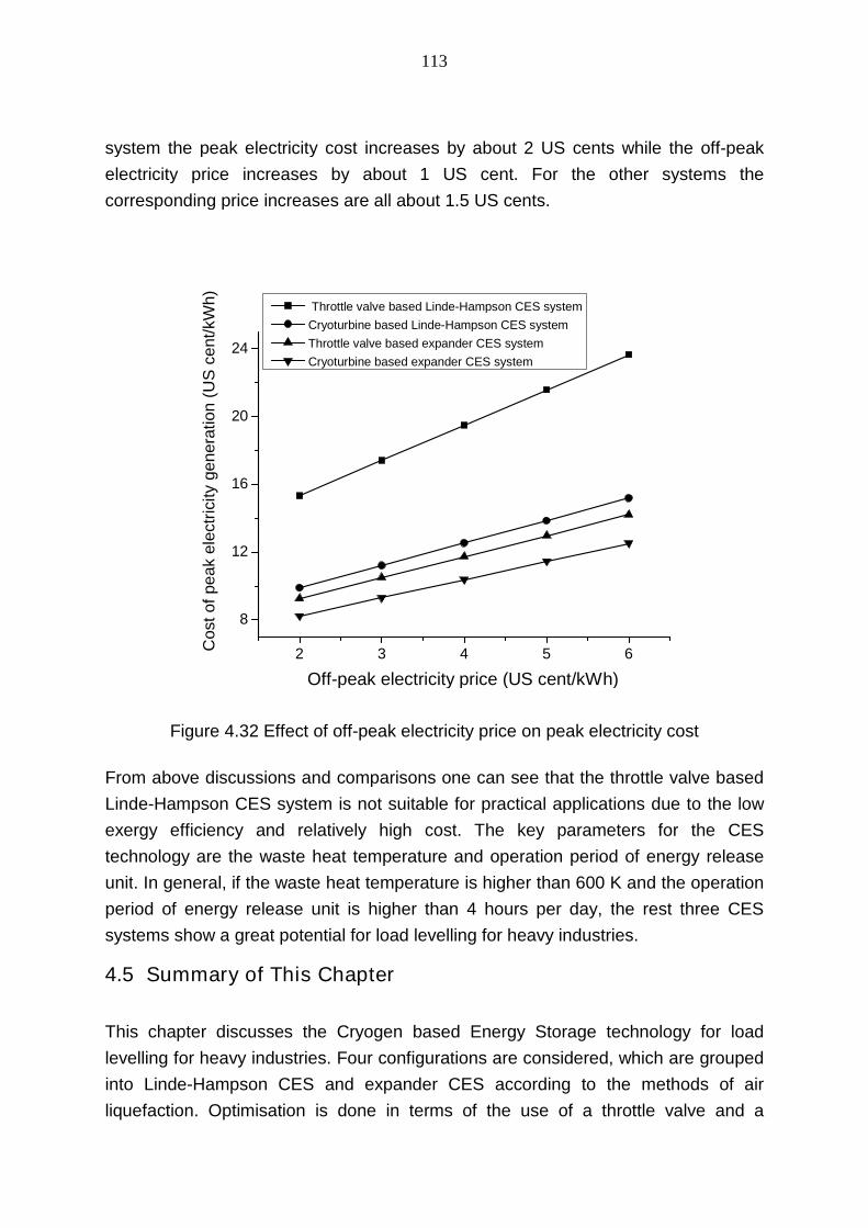
113

system the peak electricity cost increases by about 2 US cents while the off-peak

electricity price increases by about 1 US cent. For the other systems the

corresponding price increases are all about 1.5 US cents.

2 3 4 5 6

8

12

16

20

24

Off-peak electricity price (US cent/kWh)

Cost

of

peak

ele

ctr

icity

genera

tion

(US

cent/

kW

h)





Figure 4.32 Effect of off-peak electricity price on peak electricity cost

From above discussions and comparisons one can see that the throttle valve based

Linde-Hampson CES system is not suitable for practical applications due to the low

exergy efficiency and relatively high cost. The key parameters for the CES

technology are the waste heat temperature and operation period of energy release

unit. In general, if the waste heat temperature is higher than 600 K and the operation

period of energy release unit is higher than 4 hours per day, the rest three CES

systems show a great potential for load levelling for heavy industries.


This chapter discusses the Cryogen based Energy Storage technology for load

levelling for heavy industries. Four configurations are considered, which are grouped

into Linde-Hampson CES and expander CES according to the methods of air

liquefaction. Optimisation is done in terms of the use of a throttle valve and a

114

cryoturbine as the expansion component in the liquid formation process.

Thermodynamic studies show that the expander CES can give higher round trip

efficiency although its configuration is much complicated. The results also suggest

the use of cryoturbine instead of a throttle valve lead to a significant improvement on

the round trip efficiency from about 22% to 37% for the Linde-Hampson CES and

from about 40% to 45% for the expander CES under the baseline conditions.

A dimensionless parameter named Effective Heat Transfer Factor is introduced for

assessing the performance of the heat exchanger network. The treads of such a

parameter roughly agree with those of the round trip efficiency in the optimisation

process, from about 0.12 to 0.28 for the cryoturbine based Linde-Hampson CES and

from about 0.14 to 0.34 for the cryoturbine based expander CES under the baseline

conditions. This indicates that the efficient heat exchanger network is an important

factor to improve the round trip efficiency.

Economic analyses have been carried out for the optimised CES systems. It reveals

that the throttle valve based Linde-Hampson CES system is not suitable for practical

applications. The other three systems are very competitive for load levelling for

heavy industries if the waste heat temperature and the operation period of the

energy release unit are adequately set (e.g. the waste heat temperature is higher

than 600K; the operation period is longer than 4 hours per day for peak electricity

generation).

115

Chapter 5 Cryogen based Peak-shaving Technology

5.1 Introduction

It is well known that utility companies ramp power plants up and down very

frequently to follow the end-use load demand, which changes significantly in a day. It

is also understood that the peak demand only lasts for a few hours in a day, which

often occurs at the end of the daytime when there is superposition of commercial,

industrial, public lighting and residential uses [178, 179]. As the difference between

the peak and off-peak loads is significant, it is very expensive and technically

challenging for the power companies to deal with the demand-supply mismatch. As a

consequence, electrical industry must develop new technologies to meet the highest

peak demand of the year at any given moment and operate within a just-in-time

framework that follows the variable end-use demands. Currently two Supply Side

Management (SSM) technologies are often used to address the issue:

Peaking power plants or ‘Peakers’ are the power stations provide power to

electrical grids for peak demands. Natural gas fuelled power stations and

hydropower have a rapid startup and are therefore often utilized at peak

demand times.

Grid energy storage (also called large-scale energy storage) refers to the

methods used to store electricity in large-scale within an electrical power grid.

As mentioned before Pumped Hydroelectric Storage (PHS) and Compressed

Air Energy Storage (CAES) are capable to provide very large energy storage

deliverability (above 100 MW with single unit).

However building peaking power plants has a big issue in terms of costs because of

their short operating time and high fuel costs [180, 181]. On the other hand most grid

energy storage technologies are still under the developing stage except for PHS and

CAES systems. However, as mentioned before the major barrier for the

implementations of PHS and CAES is their dependence on favourable geo-

conditions which are not always available. Recently the integration technology of

CES and natural gas fuelled power generation had been proposed by Hitachi Ltd

(Japan) [182] and Expansion Energy LLC (USA) [183]. However their systems are

the extension of compressed air energy storage technology and liquid air is only

used to produce compressed air for the combustion process. As liquid air carries

116

much more exergy than compressed air the excessive cryogenic energy will be lost

in the energy extraction process, leading to an inefficient process.

In this paper, a new peak-shaving technology with CES and CO2 capture is

proposed. Such a technology uses cryogen (liquid nitrogen and oxygen) as the

energy carrier and natural gas (or alternative gaseous fuels, e.g. from gasification of

coal) as the fuel for peak power generation. The working principle is schematically

shown in Figure 5.1. Off-peak electricity is used to produce liquid nitrogen and

oxygen in an air separation and liquefaction unit (ASU). At peak hours, natural gas or

alternative gas is burned by oxygen from the ASU (oxy-fuel combustion) to generate

electricity in gas turbine power plant. CO2 produced is then captured from the flue

gas in the form of dry ice. The remaining gas mixture is then sent back to the

combustor in gas turbine power plant after recompressed to the combustion

pressure. Liquid nitrogen produced in the ASU not only serves as an energy storage

medium but also supplies the high grade cold energy for CO2 separation. In addition,

waste heat from the tail gas can be used to superheat nitrogen in the expansion

process during power recovery to further increase the system efficiency. The

nitrogen after expansion could be used to purge the sorbent bed of the ASU dryer.

Dryer

ASU

Liquid Nitrogen

Oxygen

Natural Gas

Gas Turbine

Power Plant

Flue Gas

Power Recovery System

Dry Nitrogen

Air

Argon … H2O Dry IceNitrogen

Blending Gas

Off-peak time

Peak time

Figure 5.1 Principle diagram of the cryogen based peak-shaving technology

117

This cryogen based peak-shaving technology is far better positioned if CO2 capture

is taken into account. CO2 is one of the main greenhouse gases. Global fossil-fuelled

power generation sector generates the largest amount of CO2 emission, accounting

for about 33–40 percent of the total [184, 185]. As fossil fuelled power plants are at

fixed locations, they are much more easily to manage than other major sources of

CO2 emission including transportation, space heating and industrial processing

sectors. Should CO2 reduction be deemed necessary, it is likely that the electricity

generation sector would be required to make significant contributions [186]. For fossil

fuel powered electricity generation, oxy-fuel combustion approach appears to be

very promising for CO2 capture [187]. This requires oxygen production, which can be

done by air separation and liquefaction process. Furthermore the energy extraction

process of CES produces lot of relatively low grade cold which could be used for

condensing CO2. These arguments form the basis for the work reported in this

chapter.

This chapter is organized in the following manner. Section 5.2 gives the details of the

newly proposed process where thermodynamic analyses are also carried out.

Systematic optimisation is carried out in Section 5.3, followed by an economic

analysis in Section 5.4. Finally, a summary is given in Section 5.5.

5.2 Thermodynamic Analysis

5.2.1 Cycle Configuration

Figure 5.2 shows the process flow sheet for the newly proposed cycle, whereas the

corresponding t-s (temperature – entropy) diagram is given in Figure 5.3. The cycle

works in the following way. At off-peak hours, excessive electricity generated by the

base-load units is used to power the air separation and liquefaction (ASU) plant to

produce oxygen and liquid nitrogen while the rest of the system is powered off. The

produced oxygen and liquid nitrogen are stored in pressurized vessels and cryogenic

tanks, respectively, for generating power via a high pressure turbine (HT) and a low

pressure turbine (LT) through nitrogen expansion, and assisting combustion through

an oxy-fuel combustor (B) at peak hours.

118

~~GT HT LT C2

G

HE1 HE2 HE3

ASU

P

B

C1

WS CS

Air

Ar, …

H2O CO2

1

2

3

4

5

6

7

8 9

10

11

12

13

1415

16

17

18

19

20

2122

23 24 25

26

ASU - Air separation (liquefaction) unit

HT/LT - High/Low pressure turbines

HE - Heat exchangers

WS - Water separator

CS - CO2 separator

GT - Gas turbine

B - Combustor

C - Compressors

P - Cryogenic pump

G - Generator

Helium

CH4

O2

N2

Helium/CO2

Helium/CO2/H2O

Helium

CH4

O2

N2

Helium/CO2

Helium/CO2/H2O

CH4

Figure 5.2 The flow sheet of the proposed cycle

20 22 24 26 28 30 32 34

0

300

600

900

1200

1500

16

1513

12 9/116/8

5T(

C)

S (kJ/kgK)

4

Figure 5.3 T-S diagram for helium cycle

119

At peak hours, natural gas is compressed in the compressor C1 to the working

pressure. The working fluid then mixes with the oxygen in the combustor (B) where

combustion takes place to give high temperature and high pressure flue gas

consisting of CO2 and H2O. Combustion of the natural gas in an oxygen environment

can produce a temperature that is too high for the gas turbine (GT). To control such

a temperature, an appropriate amount of blending gas is required. Helium is selected

as the blending gas first which is mixed with the flue gas before entering the GT for

power generation through a generator (G). Note that the helium gas is not consumed

but circulates in the system; see below for details. The flue gas containing helium

from the GT then goes through a series of heat exchange processes via heat

exchangers 1 (HE1), 2 (HE2) and 3 (HE3) to recover the waste heat by passing the

heat to a nitrogen stream from the ASU; see below for details. During the heat

recovery processes, steam in the flue gas is removed via a condenser (WS),

whereas CO2 is removed in the form of dry ice through a solidification process in CS

(the triple point of CO2 is 5.718 bar and 56.6oC). As a result, the flue gas stream after

CO2 removal contains only helium. The helium stream is then cooled down further in

HE3 and compressed in compressor C2 to the working pressure, and finally goes

through further heat exchange in HE2 and HE1 before flows back to the combustor.

Note that there may be a very small amount of CO2 in the separated water stream

(WS) due to thermodynamic equilibrium, for simplification of the calculations it is

assumed that water, CO2 and helium are fully separable.

Come back to the nitrogen stream starting from the cryogenic storage tank where

liquid nitrogen is pumped to the working pressure by a cryogenic pump (P). The high

pressure liquid nitrogen is then heated in heat exchangers (HE3, HE2 and HE1 in

series) and expands in two stages via respectively a high pressure turbine (HT) and

a low pressure turbine (LT) to generate electricity. Heat exchanger 1 (HE1) serves

as an inter-heater between the two stage expansion. After expansion, the pure

nitrogen can be used to purge the sorbent bed of the ASU air dryer.

From the above, one can see that the newly proposed cycle consists of a closed-

loop topping Brayton cycle with He/CO2/H2O as the working fluid and a open-loop

bottoming nitrogen direct expansion cycle. The topping Brayton cycle can be

identified as 4 → 5 → 6 → 8 → 9 → 11 → 12 → 13 → 14 → 15 → 16 → 4, whereas

the bottoming cycle goes through 18 → 20 →21 → 22 → 23 → 24 → 25 → 26. It is

the combination of the two cycles that produce electricity at the peak hours. The

120

Brayton cycle uses a smaller amount of natural gas (then it would use without the

cryogen based system), which is burned in the pure oxygen produced by the ASU

during off-peak hours. Helium is only used to control the turbine inlet temperature

(TIT) and is circulating. The working fluid of the open cycle, nitrogen, is the actual

energy carrier of the off-peak electricity. As CO2 is captured, only water and nitrogen

are given out from the process.

5.2.2 Performance Analysis

To simplify the computation, the whole system is assumed to be in the steady state.

Further assumptions for the calculations include (see also Table 5.1 for details):

HE1 is a four-pass heat exchanger as one hot stream and three cold streams

go through it. It is used to preheat the helium stream, superheat the nitrogen

stream prior to HT and reheat the nitrogen stream between HT and LT.

HE2 and HE3 are three-pass or two-pass heat exchangers depending on the

combustion pressure for cryogenic exergy recovery. This is because after

compression the temperature of stream 13 may not low enough for CO2

and/or water separation.

The positions of the heat exchangers in the cycle and temperatures at the

inlets/outlets are selected on the basis of reducing the heat transfer

irreversibility and for separating water and CO2. This is achievable by

adjusting the flow rate ratio of natural gas and liquid nitrogen.

Natural gas contains pure methane, and the combustion is stochiometric with

CO2 and H2O as the combustion products (practically an oxygen-rich

environment is required for a complete combustion process. In this case the

additional oxygen can be used as part of blending gas). The separated water

from WS does not contain CO2.

No turbine blade cooling takes place. Oxygen from the ASU is pure and the

storage vessel is at the working pressure of the combustion.

The temperatures between HE1 and HE2 are set to be at the ambient

temperature (or with an approach temperature difference for heat transfer).

Such an assumption is realistic as the outlet flow from the Brayton cycle can

be cooled by ambient water and the cryogen can be heated by the ambient

121

water if needed. Also, the direct expansion nitrogen turbines can be heated by

water while its working temperature is lower than ambient value.

Table 5.1 Main assumptions for the calculationASU Power consumption for liquid nitrogen

production (kJ/kg)

1297 [188,

189]

Fuel compressor (C1) Isothermal efficiency (%) 88

Combustor (B)

Gas turbine (GT)

Recuperation system

Efficiency (%)

Pressure loss (%)

Inlet temperature (℃)

Isentropic efficiency (%)

Water separator working temperature (℃)

100

3

1300

88

20

CO2 separator working temperature (℃) －78

Heat exchangers pressure loss (%) 2

Approach temperature (℃) 10

Helium compressor (C2) Isentropic efficiency (%) 88

Cryogenic pump (P) Efficiency (%) 77

High pressure turbine (HT)

Low pressure turbine (LT)

Fuel

Conventional oxy-fuel combined

cycle



Methane LHV (kJ/kg)

Net LHV efficiency (%)

88

88

50,010

47 [184]

Two efficiencies are employed to assess the performance of the newly proposed

cycle. One is the exergy efficiency defined as the ratio of the exergy obtained to that

consumed:

)/()( oonnffcce EmEmEmEmW (5.1)

122

where W is the overall power output from turbines less the power consumed by thecompressors and cryogenic pump. cm , fm , nm and om are respectively the mass flow

rates of carbon dioxide, fuel (natural gas), cryogen (nitrogen) and oxygen, fE

denotes the fuel exergy, which is approximately equal to its lower heating value, and

cE , nE and oE are respectively the differences between the exergies of carbon

dioxide, cryogen and oxygen at their initial states and that at the ambient state

defined by:

)()( ,10,10 caacac SSTHHE (5.2)

)()( ,18,18 naanan SSTHHE (5.3)

)()( ,3,3 oaaoao SSTHHE (5.4)

where hi and si (i=3, 10 and 18) are respectively enthalpy and entropy at point i (seeFigure 5.2), aT , aH and aS refer respectively to the ambient temperature, the

enthalpy and the entropy under the ambient conditions, and the second subscripts c,

n and o represent carbon dioxide, cryogen (liquid nitrogen) and oxygen, respectively.

The other efficiency is the so-called electricity storage efficiency and is defined as

the ratio of increased power output of the system to the energy consumed for

cryogen production:

)/()( ooccfffs EmWmEmW (5.5)

where f is electricity generation efficiency using a conventional oxy-fuel combined

cycle and cW refers to the specific work consumption for cryogen production. In the

denominator, ooEm accounts for the compression work needed to bring oxygen from

the ASU to the working pressure in the combustor. Here the increased power output

is in comparison with the case where no cryogen is used; see late for details.

From the above, one can see that, if the mass flow rate of natural gas, the pressure

in the combustor and the pressure of the cryogen at the inlet of HE3 are given, then

the mass flow rates of helium, water, carbon dioxide and oxygen can be determined.

In this work, calculations are based on a flowrate of 1kg/s methane entering the

combustor operated at 8 bar and a cryogen pressure of 100bar at the inlet to HE3.

Under such conditions, the data in Table 5.2 are obtained, which contains the values

of temperature, pressure, flowrate and composition at different positions as shown in

123

Figure 5.2. Table 5.3 summarises the performance data of the cycle. One can see

that the total power output of the proposed system is 46.12 MW. This is

approximately twice of the power output of an oxy-fuel combined cycle based on the

LHV efficiency (23.50 MW for a natural gas flowrate of 1.0kg/s). As a consequence,

the power capacity installation of peak-load units could be halved if the newly

proposed cycle is adopted. In addition, the newly proposed cycle produces dry ice

and the exergy stored in the solids CO2 is about 0.79MW. This implies a net exergy

output of the newly proposed system at 46.91 MW, leading to an exergy efficiency of

63.29%. The calculations based on the net LHV efficiency of oxy-fuel combined

cycle show a value of the recovered power for the newly proposed cycle of 22.62

MW. This gives an electricity storage efficiency of 54.04%.

Table 5.2 Working fluid parameters of the proposed cycleNo. T (℃) P (bar) G (kg/s) Mass composition

He CO2 H2O CH4 O2 N2

1 20.0 1.0 1.0 0 0 0 1.0 0 0

2 20.0 8.2 1.0 0 0 0 0 0 0

3 20.0 8.2 4.0 0 0 0 0 1.0 0

4 1300.0 8.0 14.2 0.65 0.19 0.16 0 0 0

5 463.5 1.0 14.2 0.65 0.19 0.16 0 0 0

6 20 1.0 14.2 0.65 0.19 0.16 0 0 0

7

8

9

10

11

12

13

14

15

20

20

-78.2

-78.2

-78.2

-181.4

-41.1

-

10.0

1.0

1.0

1.0

1.0

1.0

1.0

8.4

8.4

8.3

2.3

11.9

11.9

2.8

9.2

9.2

9.2

9.2

9.2

0

0.77

0.77

0

1.0

1.0

1.0

1.0

1.0

0

0.23

0.23

1.0

0

0

0

0

0

1.0

0

0

0

0

0

0

0

0

0

0

0

0

0

0

0

0

0

0

0

0

0

0

0

0

0

0

0

0

0

0

0

0

0

0

0

124

16

18

20

21

22

23

24

25

26

453.5

-195.8

-191.4

-88.2

10

126.2

20.0

149.5

20.0

8.2

1.0

102.0

101.5

101.5

100.0

10.0

10.0

1.0

9.2

31.7

31.7

31.7

31.7

31.7

31.7

31.7

31.7

1.0

0

0

0

0

0

0

0

0

0

0

0

0

0

0

0

0

0

0

0

0

0

0

0

0

0

0

0

0

0

0

0

0

0

0

0

0

0

0

0

0

0

0

0

0

0

1.0

1.0

1.0

1.0

1.0

1.0

1.0

1.0

Table 5.3 Proposed cycle performance summaryCH4 compressor work (MW) 0.36

He compressor work (MW) 6.70

Gas turbine work (MW) 41.57

HT turbine work (MW) 5.96

LT turbine work (MW) 6.16

Cryogenic pump work (MW)

Exergy stored in solid CO2 (MW)

Exergy stored in high pressure O2 (MW)

0.51

0.79

0.72

Exergy efficiency (%) 63.29

Electricity storage efficiency (%) 54.04

Figure 5.4 shows the t-Q diagram for the heat recuperation processes in the cycle,

where Q is the normalized heat duty of heat exchangers. One can observe that the

heat load distributions are uneven across the three sets of heat exchangers and the

minimal temperature differences occur in all of the heat exchangers. The pinch

points in HE1 occur at the inlet and outlet and a position where steam starts to

condense. The pinch point in HE2 takes place at a position where CO2 starts to

freeze and the pinch point in HE3 appears at the cold inlet. An inspection of Figure

125

5.4 also indicates that heat exchange processes with large temperature differences

occur mainly at regions close to the ambient temperature. As the exergy of the

working fluid in such a condition is relatively low, its effect on the overall system

performance is expected to be small. Figure 5.5 shows a pie chart of exergy loss

distribution of the components. It can be seen that HE3 loses the highest proportion

of exergy among all the heat exchangers although it has the lowest heat load (see

Figure 5.4). This is mainly because the high grade cold exergy is used to freeze

carbon dioxide at a relative high temperature. A possible way to reduce the high

exergy loss is to use a multi-stage compression process with inter-cooling by

cryogen. Furthermore, nearly half of the exergy loss occurs in the combustion

process due to mixing of low temperature helium with high temperature combustion

products. Therefore, increasing the turbine inlet temperature would be the most

effective way to enhance the exergy efficiency of the system. In addition, Figure 5.5

also indicates that increasing the isentropic efficiency of the gas turbine will be very

effective in improving the overall performance of the system. This, however,

represents a big challenge in the field of gas turbine and is out of the scope of this

work.

-0.1 0.0 0.1 0.2 0.3 0.4 0.5 0.6 0.7 0.8 0.9 1.0

-200

-100

0

100

200

300

400

500

HE3HE2HE1

20

21 12

9/1122

6/8

16

T(

C)

Q

5

Figure 5.4 T-Q diagram for the heat exchange processes

126

P

C2HE3

HE2

HE1

LT

HTGT

44.72%20.52%1.26%

2%

7.47%

5.39%14.42%

3.8%

0.42%

B

Figure 5.5 Pie chart of exergy loss distribution(GT-Gas Turbine; B-Combustor; P-Cryogenic Pump; C-Compressors; HE-Heat Exchangers;

HT/LT-High/Low Pressure Turbines)

5.2.3 Parameter Sensitivity Analysis and Discussion

The sensitivity of four parameters are investigated, including the combustor working

pressure, the turbine inlet temperature, the cryogenic cycle topping pressure and the

approach temperature of recuperation (heat exchange) processes. The effects of

these parameters on the exergy efficiency and electricity storage efficiency are

analysed. In addition, the effects of these parameters on the net output power of the

cycle and the mass flow rate of cryogen are also investigated.

Figure 5.6 shows the effect of combustor working pressure while other parameters

are kept constant. Overall the working pressure of the combustor has a very small

effect on the exergy efficiency. An increase in the working pressure gives a small

increase in both the exergy and electricity storage efficiencies first. Both the

efficiencies reach a maximum at a pressure of ~ 7 bars, followed by a decrease in

the efficiencies with a further increase in the combustion pressure. This is mainly

because that, at pressures lower than ~ 7 bars, the mass flow rate of helium

decreases significantly with increasing combustor pressure as a result of an

127

decreased inlet temperature, leading to a decrease in the flow rate of cryogen. At

pressures above ~7 bars, the rate of decrease in the helium flowrate becomes small

and the exergy loss due to mixing of the flue gas with helium becomes more

considerable, thus leading to a gentle decrease in both the exergy and electricity

storage efficiencies. Note that the optimal combustion working pressure in the newly

proposed cycle is much lower than the conventional cycles. As is known,

manufacturing of high inlet temperature gas turbines for high pressure applications

currently represents a great challenge. It is however possible to make high inlet

temperature turbines for lower pressure applications with currently available

technologies. As a consequence, the use of the newly proposed cycle indirectly

appears to address the manufacturing challenges of gas turbines in both technical

and economic aspects as will be discussed later. It is also noted that the output

power decreases slightly with increasing the combustion working pressure. This is

because the increase of the combustion working pressure decreases the outlet

temperature of gas turbine and the amount of waste heat. As a result of thermal

balance the mass flow rate of cryogen decreases accordingly as well as the power

generated by cryogen expansion.

2 4 6 8 10 12 14 16 18 2045

50

55

60

65

30

35

40

45

50

30

35

40

45

50

Eff

icie

ncy

(%)

Combustion working pressure P4 (bar)

Exergy efficiency e

Electricity storage efficiency s

Output powerMass flow rate of cryogen

Mass

flow

rate

ofcry

ogen

(kg

/s)

Outp

utp

ow

er

(MW

)

Figure 5.6 The influence of combustion working pressure P4

128

The influence of turbine inlet temperature is illustrated in Figure 5.7, which shows

that a significant increase in both the exergy and electricity storage efficiencies and a

considerable decrease in the cryogen mass flow rate with increasing turbine inlet

temperature (TIT). However, the net power output only decreases slightly with an

increase of TIT from 1000 to 1350oC. Quantitatively, for every 100oC increase in the

TIT, the exergy efficiency increases by ~ 1%, while the electricity storage efficiency

increases by about 3%. This, again, shows that increasing the turbine inlet

temperature is a very effective way to enhance the performance of the newly

proposed system.

950 1000 1050 1100 1150 1200 1250 1300 1350 140045

50

55

60

65

30

35

40

45

50

30

35

40

45

50

Eff

icie

ncy

(%)

Turbine inlet temperature T4 (C)

Exergy efficiency e



Ma

ssflo

wra

teo

fcry

og

en

(kg

/s)

Ou

tpu

tp

ow

er

(MW

)

Figure 5.7 The influence of turbine inlet temperature T4

Figure 5.8 shows the effect of pressure of the cryogen on the performance of the

newly proposed cycle for the range of 30 and 300bar. One can see that the exergy

efficiency is approximately constant at pressures above 100 bar whereas an optimal

pressure of ~ 90 bar appears to exist at which the electricity storage efficiency is the

129

highest. Such a pressure level is easily achievable with current available

technologies.

0 50 100 150 200 250 30045

50

55

60

65

30

35

40

45

50

30

35

40

45

50

Eff

icie

ncy

(%)

Topping pressure P20 (bar)

Exergy efficiency e



Ma

ss

flo

wra

teo

fcr

yo

ge

n(k

g/s

)

Ou

tpu

tp

ow

er

(MW

)

Figure 5.8 The influence of cryogenic cycle topping pressure P20

The effect of the approach temperature of the heat exchangers on the cycle

performance is illustrated in Figure 5.9. One can observe that the exergy and

electricity storage efficiencies decrease by about 1.5% and 3%, respectively, for

every 10oC increment in the approach temperature. As a consequence, a low

approach temperature should be adopted for the newly proposed cycle, which

should also increase the thermal efficiency of the system. However, a low approach

temperature implies an increase in the heat transfer surface area and hence a higher

pressure drop, which is not considered in the current study. In addition, the increase

in the heat transfer surface area also implies an increase of the costs.

130

0 5 10 15 20 25 30 35 40 4545

50

55

60

65

30

35

40

45

50

30

35

40

45

50E

ffic

ien

cy(%

)

Approach temperature T (C)

Exergy efficiency e



Ma

ssflo

wra

teo

fcr

yog

en

(kg

/s)

Ou

tpu

tp

ow

er

(MW

)

Figure 5.9 The influence of approach temperature ∆T of the recuperation system

The above sensitivity analyses show that the newly proposed cycle is likely to give

an optimal performance at a relatively low combustor working pressure (~7bar) and

medium cryogenic cycle topping pressure (~ 90bar). These pressure levels are much

lower than those currently used in the conventional cycles. The analyses also show

that an increase in the turbine inlet temperature and a decrease in the approach

temperature of the heat exchanging processes are very effective to enhance the

overall performance. From the practical point of view, the above operating

conditions are relatively easily to achieve as high temperature gas turbines are

available for low to medium pressures operations. Furthermore it is also found that

the mass flowrate of liquid nitrogen consumed by the system is about seven times as

that of required oxygen. This indicates there will be excess oxygen if the air is fully

separated in the ASU unit.

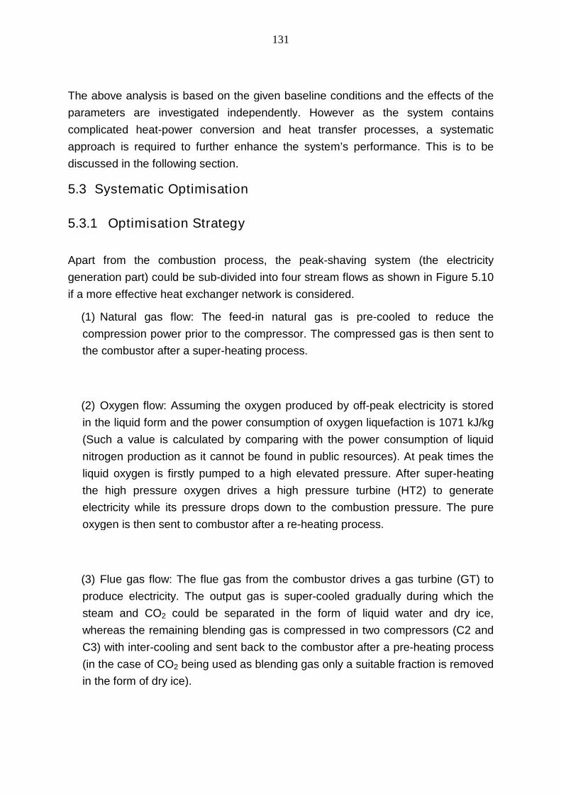
131

The above analysis is based on the given baseline conditions and the effects of the

parameters are investigated independently. However as the system contains

complicated heat-power conversion and heat transfer processes, a systematic

approach is required to further enhance the system’s performance. This is to be

discussed in the following section.

5.3 Systematic Optimisation

5.3.1 Optimisation Strategy

Apart from the combustion process, the peak-shaving system (the electricity

generation part) could be sub-divided into four stream flows as shown in Figure 5.10

if a more effective heat exchanger network is considered.

(1) Natural gas flow: The feed-in natural gas is pre-cooled to reduce the

compression power prior to the compressor. The compressed gas is then sent to

the combustor after a super-heating process.

(2) Oxygen flow: Assuming the oxygen produced by off-peak electricity is stored

in the liquid form and the power consumption of oxygen liquefaction is 1071 kJ/kg

(Such a value is calculated by comparing with the power consumption of liquid

nitrogen production as it cannot be found in public resources). At peak times the

liquid oxygen is firstly pumped to a high elevated pressure. After super-heating

the high pressure oxygen drives a high pressure turbine (HT2) to generate

electricity while its pressure drops down to the combustion pressure. The pure

oxygen is then sent to combustor after a re-heating process.

(3) Flue gas flow: The flue gas from the combustor drives a gas turbine (GT) to

produce electricity. The output gas is super-cooled gradually during which the

steam and CO2 could be separated in the form of liquid water and dry ice,

whereas the remaining blending gas is compressed in two compressors (C2 and

C3) with inter-cooling and sent back to the combustor after a pre-heating process

(in the case of CO2 being used as blending gas only a suitable fraction is removed

in the form of dry ice).

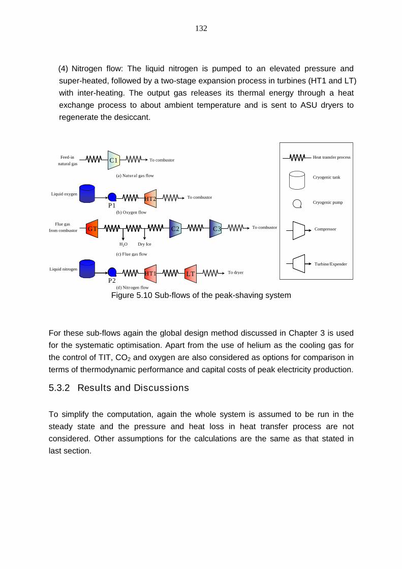
132

(4) Nitrogen flow: The liquid nitrogen is pumped to an elevated pressure and

super-heated, followed by a two-stage expansion process in turbines (HT1 and LT)

with inter-heating. The output gas releases its thermal energy through a heat

exchange process to about ambient temperature and is sent to ASU dryers to

regenerate the desiccant.

Feed-in

natural gasTo combustor

Flue gas

from combustorTo combustor

Liquid nitrogen

Liquid oxygenTo combustor

To dryer

H2O Dry Ice

(a) Natural gas flow

(d) Nitrogen flow

(c) Flue gas flow

(b) Oxygen flow


Cryogenic tank

Turbine/Expender

Compressor

Cryogenic pump

C1

HT2

GT C2 C3

LTHT1

P1

P2

Figure 5.10 Sub-flows of the peak-shaving system

For these sub-flows again the global design method discussed in Chapter 3 is used

for the systematic optimisation. Apart from the use of helium as the cooling gas for

the control of TIT, CO2 and oxygen are also considered as options for comparison in

terms of thermodynamic performance and capital costs of peak electricity production.

5.3.2 Results and Discussions

To simplify the computation, again the whole system is assumed to be run in the

steady state and the pressure and heat loss in heat transfer process are not

considered. Other assumptions for the calculations are the same as that stated in

last section.

133

0 10 20 30 40 50 600.50

0.55

0.60

0.65

0.70

0.75

Exerg

yE

ffic

iency

Generations

HeliumOxygenCO2

Figure 5.11 Exergy efficiencies versus number of generations using differentblending gases

The exergy efficiency for the different blending gases as a function of the

optimisation process is shown in Figure 5.11. It can be seen that the exergy

efficiency with helium increases from 64% to around 70%, whereas the use of

oxygen gives a very similar but a slight higher efficiency. This is easily to explain

because the two gases work completely in the gas phase region, unlike the use of

steam which involves phase change. Figure 5.12 shows the heat capacities of

helium and oxygen during the heat exchange process. One can see that the heat

capacity of helium is almost constant whereas that oxygen decreases slightly. This

means that the use of oxygen as the blending gas is able to recover more high-grade

cold and therefore make the heat transfer process more efficient. The very different

heat capacities of helium and oxygen give two different sets of optimised operating

parameters and the data are listed in Table 5.4.

134

50 100 150 200 250 3000.7

0.8

0.9

1.0

1.1

1.2OxygenCO2

Isob

aric

hea

tca

pa

citie

s(k

J/k

gK

)

Temperature (K)

50 100 150 200 250 3004.8

4.9

5.0

5.1

5.2

5.3Helium

Figure 5.12 Isobaric heat capacities vs. Temperature diagram of blending gases atambient pressure

On contrast, the optimised exergy efficiency using CO2 as the blending gas is about

10% lower than the use of helium and oxygen. This is mainly because the lowest

working temperature of CO2 has to be higher than its freezing point to avoid

solidification. As a result the cryogenic energy from the liquid nitrogen could not be

extracted efficiently due to the large temperature difference in the heat transfer

processes.

135

0 10 20 30 40 50 600.35

0.40

0.45

0.50

0.55

0.60

0.65

0.70

Ele

ctr

icity

sto

rage

eff

icie

ncy

Generations

HeliumOxygenCO2

Figure 5.13 Electricity storage efficiencies versus number of generations usingdifferent blending gases

Apart from the exergy efficiency, the calculated electricity storage efficiency is shown

in Figure 5.13 as a function of optimisation process. One can see the performance

for the use of helium and oxygen which is similar, with an efficiency of about 67%.

Such a value is much higher than other TES technologies and hydrogen storage and

is even competitive with PHS and CAES [1]. While the use of CO2 as the blending

gas only gives an electricity storage efficiency of about 50%.

Comparison of the performance of CO2 with that of helium and oxygen shows

inefficient heat transfer processes being the reason for low efficiency. As a result, the

Effective Heat Transfer Factor is used to investigate the performance of the heat

transfer processes.

Table 5.4 Key parameters of the optimized peak-shaving system using differentblending gases

Blending gas Helium Oxygen CO2

Combustion pressure (bar) 6.4 16.9 13.8

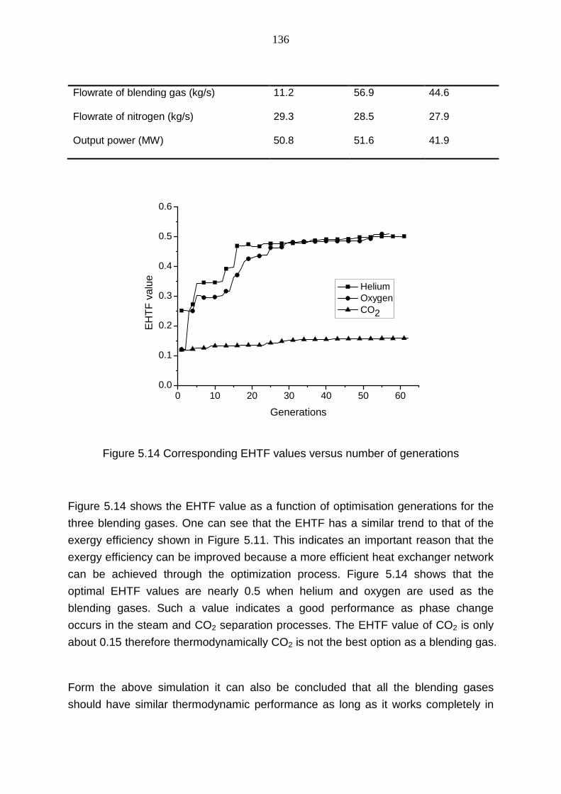
136

Flowrate of blending gas (kg/s) 11.2 56.9 44.6

Flowrate of nitrogen (kg/s) 29.3 28.5 27.9

Output power (MW) 50.8 51.6 41.9

0 10 20 30 40 50 600.0

0.1

0.2

0.3

0.4

0.5

0.6

EH

TF

valu

e

Generations

HeliumOxygenCO2

Figure 5.14 Corresponding EHTF values versus number of generations

Figure 5.14 shows the EHTF value as a function of optimisation generations for the

three blending gases. One can see that the EHTF has a similar trend to that of the

exergy efficiency shown in Figure 5.11. This indicates an important reason that the

exergy efficiency can be improved because a more efficient heat exchanger network

can be achieved through the optimization process. Figure 5.14 shows that the

optimal EHTF values are nearly 0.5 when helium and oxygen are used as the

blending gases. Such a value indicates a good performance as phase change

occurs in the steam and CO2 separation processes. The EHTF value of CO2 is only

about 0.15 therefore thermodynamically CO2 is not the best option as a blending gas.

Form the above simulation it can also be concluded that all the blending gases

should have similar thermodynamic performance as long as it works completely in

137

their gaseous region. Therefore not only helium, but also other inert gases can be

the candidates of blending gas.

5.4 Economic Analysis

5.4.1 Economic Modelling

Estimation of the capital costs as well as costs associated with owning and operating

the system at the component level is a key step to assess the competitiveness and

viability of the technology. The methodology for estimating the main components

costs and amortization factor are the same as those used in Chapter 4 and

presented in Appendix B.

It is difficult to estimate the capital cost of ASU facility from published information.

However it is reported that the cost ratio of capital charges to recover the investment

and provide a return on investment and power charges is between 0.43 and 1.0

while the operating labour costs only form a small fraction[59, 189, 190]. Personal

communication with liquefaction facility suppliers shows the capital cost is about

30,000 US$/(ton/day) (for a 500 ton/day system) which corresponds a cost ratio of

about 0.86. Therefore such a value is adopted in the following calculations.

Based on the above definition, the capital cost of peak-shaving system is expressed

as:

PS

PSPS

W

IC (5.6)

The electricity production cost of the peak-shaving system could be expressed as:

O

fI

O

OWCEmCF

WCE PS

ASUopkCHCH

PS

PS365

24144

(5.7)

Ideally the air separation and liquefaction unit should operate only at off-peak times.

Such a scenario is impracticable as it typically takes several hours for the oxygen

and nitrogen product streams to reach the desired product purities [59]. Recent

flexibility studies of cryogenic air separation technology show that a turn-down of

50% of the nominal ASU (semi base load) is achievable with the load change

velocity of 1-2% per minute [191]. However such a technology is still under

development and not fully demonstrated. Therefore in the following economic

138

analyses it is assumed the air separation and liquefaction unit operates continuously

at a constant load.

5.4.2 Results and Discussions

A peak-shaving plant with a net output power (generated power subtracts the power

consumed by ASU) of 600 MW is used as a case study for the economic analyses.

Other baseline assumptions are listed in Table 5.5.

Three peak-shaving systems using different blending gases are calculated. The

purchase prices of main components are shown in Figure 5.15. One can see that the

ASU, gas turbine and expenders (including high pressure turbines HT and low

pressure turbine LT) take the major shares of the costs for all the three systems.

Comparison of the three systems indicates that the costs of compressors and gas

turbine of the helium system is much lower than that of the other two systems. This

is because helium has a much higher heat capacity leading to a smaller mass

flowrate and combustion pressure and hence a lower capital cost. It is also seen that

the ASU and the expander costs of CO2 system is much higher than the other two

systems. This is because the exergy efficiency of CO2 system is much lower than the

other systems, which requires a higher mass flowrate of liquid nitrogen to give the

same amount of net output power.

The above discussion is based on a scenario of 2 hours peak shaving operation per

day. Increasing the operation duration will require more capacity of liquefaction unit

and hence the costs. Figure 5.16 shows the results. One can see that the capital

costs of the peak-shaving systems increase dramatically with increasing operation

hours. Even so they are much cheaper than oxy-NGCC based technology for peak

shaving when the operation time is less than 8 hours per day (see Figure 5.16). Of

particular interest is that if the operation period is lower than 2 hours, the capital cost

of the three peak-shaving systems could be lower than traditional NGCC technology

(see Figure 5.16) [184]. Again among the three peak-shaving systems the capital

cost of helium based is the lowest.

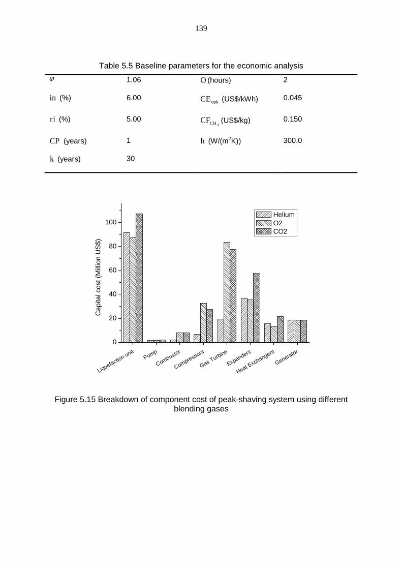
139

Table 5.5 Baseline parameters for the economic analysis

1.06 O (hours) 2

in (%) 6.00opkCE (US$/kWh) 0.045

ri (%) 5.004CHCF (US$/kg) 0.150

CP (years) 1 h (W/(m2K)) 300.0

k (years) 30

Liquefaction unit

Pump

Combustor

Compressors

Gas Turbine

Expanders

Heat Exchangers

Generator

0

20

40

60

80

100

Ca

pita

lco

st

(Mill

ion

US

$)

HeliumO2CO2

Figure 5.15 Breakdown of component cost of peak-shaving system using differentblending gases

140

0 1 2 3 4 5 6 7 8 9

200

400

600

800

1000

1200

1400

1600

Oxy-NGCC

Ca

pitalcost(U

S$

/kW

)

Operation period (hours per day)

HeliumOxygenCO2

NGCC

Figure 5.16 Effect of operation period on capital cost of peak-shaving systems

The cost of peak electricity production consists of capital cost, fuel cost and off-peak

electricity cost for the peak-shaving systems. Figure 5.17 shows the baseline costs

of peak electricity production using the three different systems, together with the

NGCC and oxy-NGCC. For all the three peak-shaving systems the capital cost is the

dominant factor, followed by the cost of off-peak electricity. The fuel only takes a

small fraction. The peak electricity costs of the three peak-shaving systems

considered in this work are more or less the same as that of the NGCC system, but

they are much lower than that of the oxy-NGCC system.

Similarly to the capital costs, the peak electricity costs are affected by the operation

period. Figure 5.18 shows the results. One can see that the costs of peak-shaving

systems decrease first with increasing of operation hours, but then levels off once

the operation period is longer than 4 hours a day. This is mainly because of the

capital costs of liquefaction unit as discussed before. On the other hand the peak

electricity costs of NGCC and oxy-NGCC decrease monotonously with the increase

of operation hours. The comparison indicates that the peak-shaving systems are

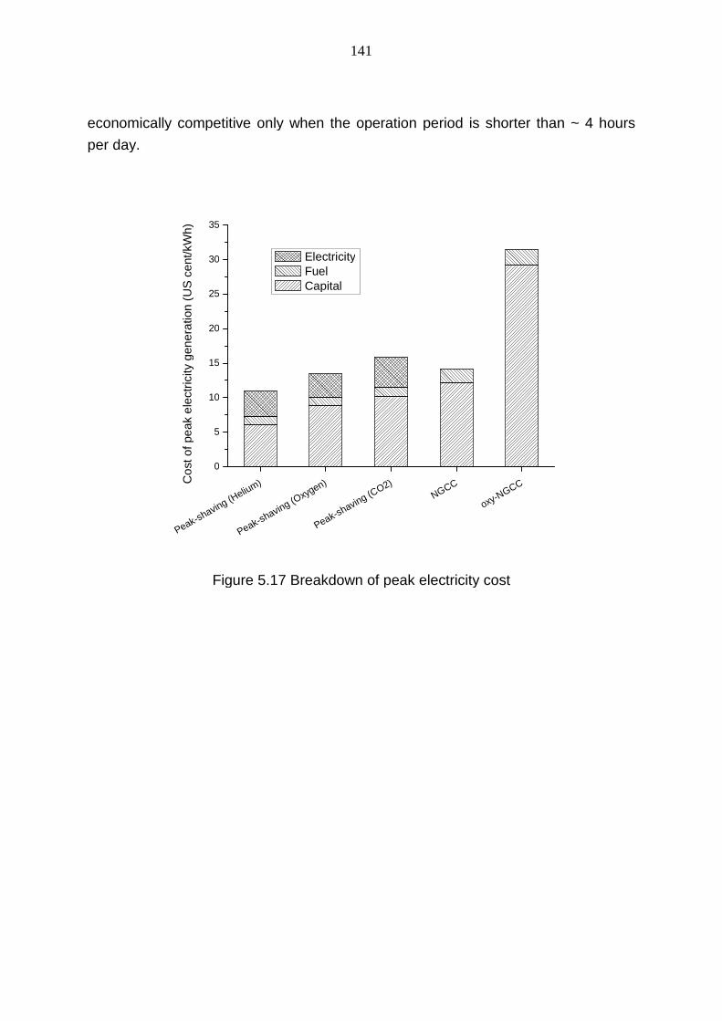
141

economically competitive only when the operation period is shorter than ~ 4 hours

per day.

Peak-shaving (Helium)

Peak-shaving (Oxygen)

Peak-shaving (CO2)

NGCC

oxy-NGCC

0

5

10

15

20

25

30

35

Co

sto

fpe

ak

ele

ctr

icity

gen

era

tion

(US

ce

nt/kW

h)

ElectricityFuelCapital

Figure 5.17 Breakdown of peak electricity cost

142

0 1 2 3 4 5 6 7 8 90

5

10

15

20

25

30

35

Co

sto

fpe

ak

ele

ctr

icity

gen

era

tio

n(U

Sce

nt/kW

h)

Operation period (hours per day)

HeliumOxygenCO2

NGCCoxy-NGCC

Figure 5.18 Effect of operation period on peak electricity cost

The effects of off-peak electricity and fuel costs on the peak electricity cost are

compared and are shown in Figure 5.19 and Figure 5.20, respectively. A linear

relationship is seen before the peak and off-peak electricity costs, the rate (slope) of

the increase is much smaller than that of the dependence on the operation period.

Figure 5.20 also shows that costs of the NGCC and oxy-NGCC technologies are

more sensitive to the fuel costs than the three systems considered in this work.

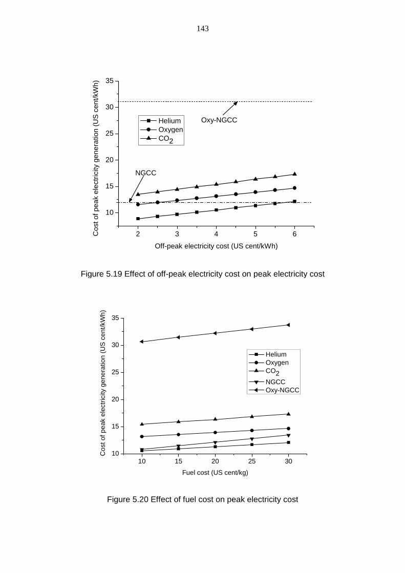
143

2 3 4 5 6

10

15

20

25

30

35

Co

sto

fpe

ak

ele

ctr

icity

ge

ne

ratio

n(U

Sce

nt/kW

h)

Off-peak electricity cost (US cent/kWh)

HeliumOxygenCO2

NGCC

Oxy-NGCC

Figure 5.19 Effect of off-peak electricity cost on peak electricity cost

10 15 20 25 3010

15

20

25

30

35

Co

stofp

eak

ele

ctr

icity

ge

ne

ratio

n(U

Sce

nt/kW

h)

Fuel cost (US cent/kg)

HeliumOxygenCO2

NGCCOxy-NGCC

Figure 5.20 Effect of fuel cost on peak electricity cost

144

From the above discussion, one can see that the cryogen based peak-shaving

technology is very competitive especially for short peak durations. If the operation

time is less than 3 hours a day, both the capital and the peak electricity costs are

comparable with the NGCC, but are much lower than the oxy-NGCC. Particularly if

helium is used as the blending gas the costs of the peak-shaving system is even

lower than that of NGCC even with CO2 captured from the flue gas.

It should be noted that there are two challenges associated with the use of helium as

the blending gas. The first is the unavoidable leakage in the water and CO2

separation processes, which requires helium makeup and hence the increase in the

operation cost as helium is expansive. The second is that it requires a new gas

turbine for the working fluid consisting of a mixture of helium, CO2 and steam. Using

oxygen as the blending gas the makeup cost for leakage is not considered as a main

challenge as oxygen is produced in the air separation and liquefaction system and

the cost is low. As oxygen has similar thermodynamic properties as air it is expected

that the traditional gas turbine could be used directly. Of course, a disadvantage of

using oxygen is associated safety related issue. But this should be manageable

using today’s technologies.

Selecting CO2 as the blending gas the safety and leakage issues are greatly

decreased. However the capital cost for peak electricity production will increase as

discussed above. Further work is needed to evaluate the leakage and safety issues,

particularly during the heat recovery and CO2 separation processes.


A new peak-shaving system integrating peak electricity generation, electrical energy

storage and CO2 capture is proposed. Such a system combines a direct open

nitrogen expansion cycle with a natural gas-fuelled closed Brayton cycle.

Thermodynamic analyses are carried out on the system under the baseline

conditions of 1 kg/s natural gas, combustor operating pressure of 8 bar and cryogen

topping pressure of 100 bar. It is found that the exergy efficiency is as high as 64%

under the baseline conditions, whereas the corresponding electricity storage

efficiency is about 54%. The sensitivity analyses indicate that the above baseline

performance can be enhanced by increasing the gas turbine inlet temperature,

145

decreasing the approach temperature of the heat exchange process, operating the

combustor at an optimal pressure (~7 bar) and operating the cryogen topping

pressure at ~ 90 bar. Further enhancement can be achieved by increasing the

isentropic efficiency of the gas turbine and the liquefaction processes. The results

also suggest that the fuel consumption could be reduced by half by using the newly

proposed system.

A global thermodynamic optimisation is carried out for the new proposed system.

Helium, oxygen and CO2 are used as the blending gas for the system. Helium and

oxygen are found to have nearly the same thermodynamic performance with exergy

efficiency increasing from 64% to about 70% and the corresponding electricity

storage efficiency increasing from 54% to about 67%. On contrast the optimal

efficiency of CO2 system is much lower due to the limitation of the lowest working

temperature of CO2 for avoiding solidification.

Economic analyses show that both the capital and peak electricity costs of the peak-

shaving systems are comparable with the NGCC which are much lower than the oxy-

NGCC if the operation period is relatively short. Among the three peak-shaving

systems, the use of helium as the blending gas has the lowest costs due to the

lowest combustion pressure and mass flowrate.

Capital costs are found to be the dominant factor for all the peak systems considered

and the ASU takes a large share. Therefore the costs of the peak-shaving systems

could be reduced by taking the following measures:

Decreasing the cost of the ASU. The data used for costing in this work is

based on a liquefaction system with a capacity of 500 ton per day. Reduction

is possible by increasing the capacity.

Variable load operation of air liquefaction unit. As the air liquefaction unit

operates continuously it consume part of the power generated by the peak-

shaving system. If the liquefaction unit could run at a variable load (e.g. semi

base load at peak time) the capital cost of other components could be

decreased. Furthermore variable load operations could follow the real price

change of off-peak electricity and save the operating cost.

146

Excess oxygen. It is found that the ratio of liquid oxygen and nitrogen

consumed by the peak-shaving system is about 1:7. For fully separated air by

the ASU, there will be excess oxygen. This part of oxygen can be used as

process gas if the system is installed close to a process plants such as

chemical and iron and steel-making plants. The excess oxygen can also be

sold as products.

147

Chapter 6 Solar-Cryogen Hybrid Power System

6.1 Background

Energy and environment are two of the most concerning issues in the current world.

For over a century cheap, plentiful fossil energy has been supporting the

industrialization and the increasingly higher living standards. However, increasing

energy demand particularly in developing countries implies depletion of the fossil fuel

resources at a rapid rate. In the meantime, the use of fossil fuels continues to cause

environmental degradation. All these call for the use of new and renewable energy

resources. Currently, renewable energy contributes to only 11% of the world primary

energy and this is expected to increase to 60% by 2070 [192]. Solar energy is one of

the most promising clean and non-depleting sources that is able to fulfill the

increasing energy demands. Apart from direct heating applications, solar energy can

be converted to electrical energy in two main ways. One is through solar cells

(photovoltaic technology), which convert solar radiation to electrical energy directly.

The other is via an indirect solar thermal route, which converts the solar radiation to

thermal energy by means of solar collectors or concentrators followed by electricity

generation through a conventional thermal process. Solar cells are most suitable for

small scale low-power applications, while solar thermal power plants are often the

best option for large-scale and grid-connected systems [193, 194].

The work reported in this chapter is concerned about improving the indirect power

generation via the solar thermal route in a Solar Thermal Power Plant (STPP). The

STPP is a conventional power station that obtains all or parts of its thermal energy

load by concentrating solar radiation, producing high temperature solar heat to

activate a Rankine power cycle. In this process the concentrated solar radiation does

not heat the working fluid of the power cycle directly but uses a solar energy carrier,

which transport the solar radiation to a storage vessel and also transfer the heat to

the working fluid. The use of heat carrier has an advantage of more precise control

of quality and quantity of vapour of the working fluid according to needs. In addition,

the use of storage and a heat carrier also enables the mass flow rate of the working

fluid to be optimized independent of the fluctuations either or both of the load and

solar radiation [22, 195]. The stored thermal energy can be used to either pre-heat

water/steam in steam cycle power plants [196] or super-heat the steam in combined

cycle power plants [25, 197] or even produce steam directly in Direct Steam

148

Generation (DSG) [22, 23]. Generally in these cycles water/steam or other organic

liquids are selected as the working fluid and the solar energy is stored in the form of

high temperature sensible heat. It is therefore less efficient when taking the behavior

of the solar thermal energy carrier into account due to temperature glide

mismatching between the solar thermal energy carrier and the working fluid.

This part of work is also concerned with efficient extraction of cold energy from

cryogens which has been one of the main objectives of this work. Cryogenic energy

extraction is of importance not only for CES but also for the fast developing liquefied

natural gas (LNG) industry. For example it is estimated that the amount of LNG

imported to China is 20 million tons by end of 2010 [171]. However, efficient recovery

of the cryogenic energy is a challenge during the evaporation process without

providing some heat to increase the temperature difference. This constitutes the

primary motivation of working on integrating the solar thermal and cryogen power

systems. This integration, as will be seen later, is able to give a higher overall energy

efficiency and in the meantime alleviate the environmental impact of the re-

gasification processes of cryogens.

For achieving the above objective, an integrated solar-cryogen hybrid power system

is proposed and analyzed. A solar thermal power system and a cryogen fuelled

power system are used as the benchmarks to evaluate the performance of the newly

proposed integrated system.

6.2 Thermodynamic Consideration and Modelling Methodologies

In this section, analyses will be carried out on the three power systems of (i) Solar

thermal power system, (ii) Cryogen fuelled power system and (iii) Solar-cryogen

hybrid power system, where (i) and (ii) are used as the benchmarks for evaluating

third system - the integrated power system proposed in this work.

6.2.1 Solar Thermal Power System

A solar thermal power system usually involves focusing sunlight on a small area to

create a high-temperature heat source. A thermal energy carrier is often used to

transport the heat and pass the heat to the working fluid via a heat exchange system.

Table 6.1 shows a list of frequently-used high temperature thermal energy carriers

[25, 198], which are either pure or mixtures of different thermal fluids. Figure 6.1

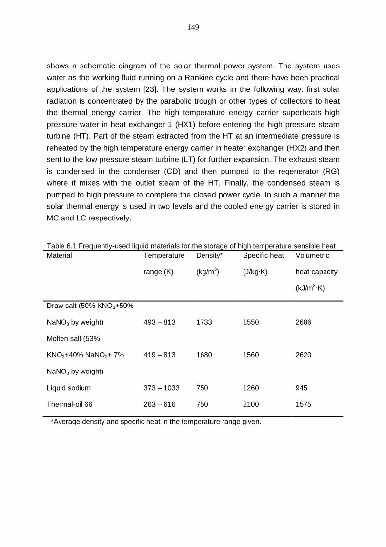
149

shows a schematic diagram of the solar thermal power system. The system uses

water as the working fluid running on a Rankine cycle and there have been practical

applications of the system [23]. The system works in the following way: first solar

radiation is concentrated by the parabolic trough or other types of collectors to heat

the thermal energy carrier. The high temperature energy carrier superheats high

pressure water in heat exchanger 1 (HX1) before entering the high pressure steam

turbine (HT). Part of the steam extracted from the HT at an intermediate pressure is

reheated by the high temperature energy carrier in heater exchanger (HX2) and then

sent to the low pressure steam turbine (LT) for further expansion. The exhaust steam

is condensed in the condenser (CD) and then pumped to the regenerator (RG)

where it mixes with the outlet steam of the HT. Finally, the condensed steam is

pumped to high pressure to complete the closed power cycle. In such a manner the

solar thermal energy is used in two levels and the cooled energy carrier is stored in

MC and LC respectively.

Table 6.1 Frequently-used liquid materials for the storage of high temperature sensible heat

Material Temperature

range (K)

Density*

(kg/m3)

Specific heat

(J/kg∙K)

Volumetric

heat capacity

(kJ/m3∙K)

Draw salt (50% KNO3+50%

NaNO3 by weight) 493 – 813 1733 1550 2686

Molten salt (53%

KNO3+40% NaNO2+ 7%

NaNO3 by weight)

419 – 813 1680 1560 2620

Liquid sodium 373 – 1033 750 1260 945

Thermal-oil 66 263 – 616 750 2100 1575

*Average density and specific heat in the temperature range given.

150

HX1 HX2

CD

HT

RG

LT

SC

LC

HC

P2

P1

MC

CD – Condenser

RG – Regenerator

P – Pump

HC – High Temperature Carrier Tank

MC – Intermediate Temperature Carrier Tank

LC – Low Temperature Carrier Tank

HX – Heat Exchanger

HT – High Pressure Turbine

LT – Low Pressure Turbine

SC – Solar Collector

P3

P4

P5

Figure 6.1 Configuration of a solar thermal power system

The thermal efficiency of a solar collector is given as [199]:

b

S

SC

aSC

b

S

SC

SC

bS

SC

CSCSCSCSC

EC

TTUF

EC

TF

EC

TFF

dIR

dQT

44

, )()()(

(6.1)

where Q is usable process heat and IR is the total irradiance of the collector.

SCF)( , SCF)( and SCF)( are respectively the absorption term coefficient, the

emission term coefficient and the absorber loss term coefficient of solar collector. is the Stefan–Boltzmann constant, equals to 5.67 10-8W/(m2∙K4) , SCUF is the

convection heat loss coefficient of solar collector, T is the fluid temperature, CSCT is

the cover temperature, aT is the ambient temperature, SCC is the concentration ratio,

bS E is the direct radiation, d

SSb

S EEE with dS E the diffusion radiation and ES the

global irradiance, 4sS

S TfE with Sf being the dilution factor which can be assumed

to be wavelength independent. In case of concentrated radiation the diffuse solar

part in the incident global radiation can be omitted, one has EE Sb

S . Integrating

Equation (6.1) from State 1 to State 2, the total irradiance of the collector can be

obtained as:

2

1 ,

1T

T SC

dQT

IR

(6.2)

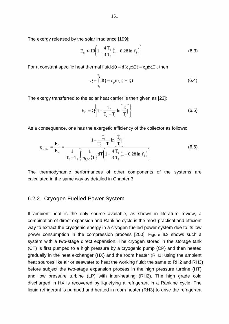
151

The exergy released by the solar irradiance [199]:

S

S

asi f

T

TIRE ln28.01

3

41 (6.3)

For a constant specific heat thermal fluid dTmcTmcddQ pp )( , then

2

1

)( 12

T

T

p TTmcdQQ (6.4)

The exergy transferred to the solar heat carrier is then given as [23]:

1

2

12

0 ln1T

T

TT

TQEQ (6.5)

As a consequence, one has the exergetic efficiency of the collector as follows:

2

1

ln28.013

41

11

ln1

,12

1

2

12, T

T

S

S

a

SC

a

si

Q

SC

fT

TdT

TTT

T

T

TT

T

E

E

(6.6)

The thermodynamic performances of other components of the systems are

calculated in the same way as detailed in Chapter 3.

6.2.2 Cryogen Fuelled Power System

If ambient heat is the only source available, as shown in literature review, a

combination of direct expansion and Rankine cycle is the most practical and efficient

way to extract the cryogenic energy in a cryogen fuelled power system due to its low

power consumption in the compression process [200]. Figure 6.2 shows such a

system with a two-stage direct expansion. The cryogen stored in the storage tank

(CT) is first pumped to a high pressure by a cryogenic pump (CP) and then heated

gradually in the heat exchanger (HX) and the room heater (RH1: using the ambient

heat sources like air or seawater to heat the working fluid; the same to RH2 and RH3)

before subject the two-stage expansion process in the high pressure turbine (HT)

and low pressure turbine (LP) with inter-heating (RH2). The high grade cold

discharged in HX is recovered by liquefying a refrigerant in a Rankine cycle. The

liquid refrigerant is pumped and heated in room heater (RH3) to drive the refrigerant

152

turbine (RT) to produce more power. The commonly used refrigerant, propane, is

selected as the working fluid for the Rankine cycle in this section. Again the

mathematical formulae detailed in Chapter 3 are used to evaluate the

thermodynamic performance of the components in this system.

CP HP

RT

LPCT

HX

P

Exhaust gas

HP – High Pressure Turbine

LP – Low Pressure Turbine

RT – Refrigerant Turbine

P – Pump

RH – Room Heater

CT -- Cryogen Tank

CP – Cryogenic Pump


RH1 RH2

RH3

CP HP

RT

LPCT

HX

P

Exhaust gas

HP – High Pressure Turbine

LP – Low Pressure Turbine

RT – Refrigerant Turbine

P – Pump

RH – Room Heater

CT -- Cryogen Tank



RH1 RH2

RH3

Figure 6.2 Configuration of cryogen fueled power system

6.2.3 Solar-Cryogen Hybrid Power System

The hybrid system proposed in this chapter integrates the solar thermal power cycle

and the cryogen fuelled power cycle and the cryogen itself is used as the common

working fluid. Figure 6.3 illustrates such a system. One can see that the hybrid

system consists of three parts: an open cycle of cryogen direct expansion, a closed

Brayton cycle for full extraction of cryogenic energy and a solar energy collection and

storage unit to capture the solar energy and provide the heating source for both the

cycles. In this system the closed Brayton cycle shares the intermediate pressure

turbine (IT) and low pressure turbine (LT) with the direct expansion cycle to simplify

the configuration while the cryogen is also used as the working fluid of the Brayton

cycle. The cold energy released by the cryogen direct expansion is recycled by the

Brayton cycle through a heat transfer process in HX1. Similarly to the solar thermal

power system, the solar thermal energy (the heat source) is extracted at two levels:

the superheating process between State 14 and State 16 corresponding respectively

to the high temperature and low temperature carriers and the inter-heating process

between State 14 and State 15 corresponding respectively to the high temperature

153

and intermediate temperature carriers. Comparing with the solar thermal power

system, an additional compressor is used in the hybrid system.

CP

HX1

HX2 HX5HX4HX3HT IT LT AC

SC

CT

LC

HC

P2

P1

Exhaust gas

MC

IT – Intermediate Pressure Turbine

LT – Low Pressure Turbine

AC – Adiabatic Compressor

SC – Solar Collector

P – Pump

HC – High Temperature Carrier Tank

MP – Intermediate Temperature Carrier Tank

LC – Low Temperature Carrier Tank

CT -- Cryogen Tank



HT – High Pressure Turbine

12

3 4 56

7 8

9

10

111

12

13

14

15

16

Figure 6.3 Configuration of a cryogen-solar hybrid power system

6.3 Parametric Optimisation and System Analysis

Based on the power systems detailed above, parametric optimisation is carried out.

The following exergy efficiencies are selected as the objective functions for the

optimisation:

si

netSP

E

W (6.7)

ASU

netCF

W

W (6.8)

ASUsi

netSCH

WE

W

(6.9)

154

where SP , CF and SCH are respectively the exergy efficiencies of the solar thermal

power system, the cryogen fuelled power system and the solar-cryogen hybrid powersystem, netW is the net power output (equal to the turbine output power subtracting

the power consumed by compression and pumping processes) and ASUW is the

power consumed by the cryogen production process.

Liquid nitrogen is taken as an example of the working cryogen in the parametric

optimization and the solar energy carrier is assumed to have a constant specific heat.

Other data used in the simulations are summarized in Table 6.2 [23, 92, 199, 201]

(here the assumption of turbine isentropic efficiency is slightly higher than the

previous assumptions as the inlet temperature in this system is more closer to the

ambient as a result the thermal loss should be lower than traditional gas turbines or

cryogenic turbines). The overall optimal performance of the three systems is given in

Table 6.3. From the table, one can see that the exergy efficiency of the hybrid power

system is much higher than the solar thermal and cryogen fuelled only power

systems. Given the same energy source, the net output power of the hybrid power

system is 1.0118 MW, which is almost 31% higher than that the summation of output

power of both solar thermal and cryogen fuelled power systems.

Table 6.2 Main assumptions for the parametric optimisation

Solar collector

Absorption term coefficient SCF)( 0.8

Emission term coefficient SCF)( 0.8

Absorber loss term coefficient SCF)( 0.8

Convection heat loss coefficient SCUF /Wm-2K-1 20

Cover temperature CSCT /K 300

The concentration ratio SCC 40

Cryogenic pump isentropic efficiency P 0.75

Turbine isentropic efficiency EP 0.90

Compressor isentropic efficiency CP 0.87

155

Approach temperature of heat exchanger system MATT /K 10

The wet vapour quality of steam turbine >0.9

The effective solar temperature sT/K

5,777

The dilution factor Sf 1.310-5

Ambient temperature aT /K 298.15

Ambient pressure aP / bar 1.0

Power consumption of liquid nitrogen production ASUW / (kWh/kg) 0.5

The mass flow of liquid nitrogen nm / (kg/s) 1.0

Table 6.3 Overall optimal performances of the three systemsSolar thermal

power system

Cryogen fueled

power system

Solar-cryogen

hybrid power

system

Exergy efficiency (%) 23.89 18.10 27.55

Energy

Source

Solar radiation

(MW)

2.628 0 2.628

Liquid nitrogen

(kg/s)

0 1.0 1.0

Net output power (MW) 0.4485 0.3259 1.0118

The performance improvement of the hybrid power system comes from more

efficient heat transfer processes. This can be demonstrated by the exergy analysis of

the energy conservation processes using a graphical representation method named

energy utilization diagram (EUD). In the EUD method an intensive parameter called

availability factor or energy level AL is introduced as an indicator of the potential of

the energy donated and accepted by the processes [202]:

156

H

EAL

(6.10)

Defining a process that releases energy as an ‘energy donor (ED)’ and a process

that receives energy as an ‘energy acceptor (EA)’, the exergy loss of the processes

can then be given by:

dHALALALALHEEXL eaedieaiedii )()( ,, (6.11)

By plotting the availability factor of the energy donating and accepting processes

against the transferred energy, the amount of exergy loss in the system can be

obtained as the area between the two curves.

Figure 6.4 and Figure 6.5 show the EUD representations of the optimised cryogen

fuelled and hybrid power systems, respectively. One can see the exergy loss in the

heat exchangers and room heaters of the hybrid power system is significantly lower

than that in the cryogen fuelled power system. There are two reasons for this. First,

the use of the Brayton cycle in the hybrid system enables a much more efficient heat

transfer to recover the high grade cold energy due to better temperature glide

matching between heat addition and heat rejection. Second, the outlet temperature

of the expanded gas is increased as the compressed gas is superheated by the solar

thermal energy prior to entering the turbines. Therefore the exergy loss in the

exhaust gas is reduced. Meanwhile, the use of cryogen as the working fluid is

beneficial for the solar thermal energy utilization. This can be understood from Table

6.4, which shows that the critical temperatures and pressures of nitrogen are much

lower than that of the steam. As a consequence, supercritical cycles are much easily

to achieve using the cryogen. Listed in Table 6.4 also includes the critical properties

of methane, which, as will be discussed in the following section in terms of

applications, also gives much better performance than the use of steam as the

working fluid.

Table 6.4 Critical temperature and pressure for water, nitrogen and methaneWater/Steam Nitrogen Methane

Critical temperature (K) 647 126 190

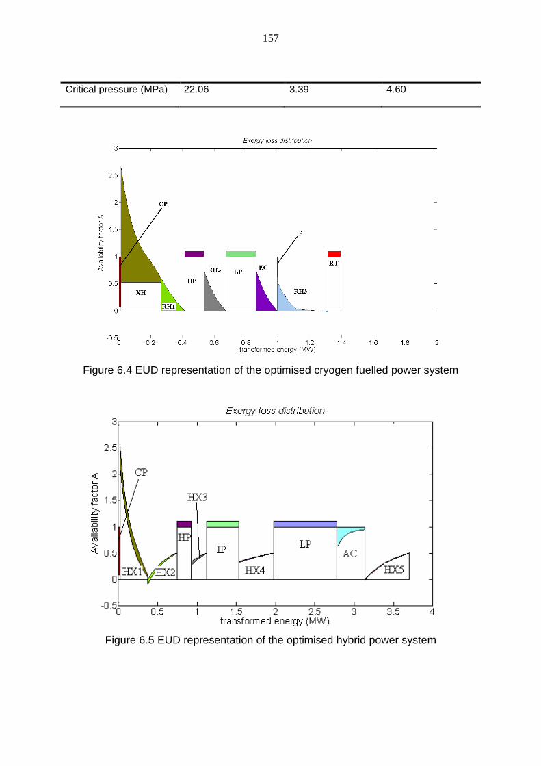
157

Critical pressure (MPa) 22.06 3.39 4.60

Figure 6.4 EUD representation of the optimised cryogen fuelled power system

Figure 6.5 EUD representation of the optimised hybrid power system

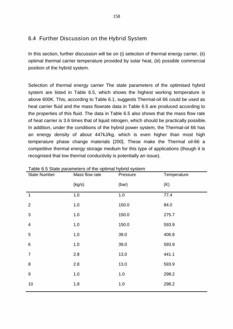
158

6.4 Further Discussion on the Hybrid System

In this section, further discussion will be on (i) selection of thermal energy carrier, (ii)

optimal thermal carrier temperature provided by solar heat, (iii) possible commercial

position of the hybrid system.

Selection of thermal energy carrier The state parameters of the optimised hybrid

system are listed in Table 6.5, which shows the highest working temperature is

above 600K. This, according to Table 6.1, suggests Thermal-oil 66 could be used as

heat carrier fluid and the mass flowrate data in Table 6.5 are produced according to

the properties of this fluid. The data in Table 6.5 also shows that the mass flow rate

of heat carrier is 3.6 times that of liquid nitrogen, which should be practically possible.

In addition, under the conditions of the hybrid power system, the Thermal-oil 66 has

an energy density of about 447kJ/kg, which is even higher than most high

temperature phase change materials [200]. These make the Thermal oil-66 a

competitive thermal energy storage medium for this type of applications (though it is

recognised that low thermal conductivity is potentially an issue).

Table 6.5 State parameters of the optimal hybrid systemState Number Mass flow rate

(kg/s)

Pressure

(bar)

Temperature

(K)

1 1.0 1.0 77.4

2 1.0 150.0 84.0

3 1.0 150.0 275.7

4 1.0 150.0 593.9

5 1.0 39.0 406.8

6 1.0 39.0 593.9

7 2.8 13.0 441.1

8 2.8 13.0 593.9

9 1.0 1.0 298.2

10 1.8 1.0 298.2

159

11 1.8 1.0 94.0

12 1.8 39.0 294.4

13 1.8 39.0 593.9

14 3.6 - 603.9

15 2.1 - 451.1

16 1.5 - 304.4

Optimal thermal carrier temperature provided by solar heat The optimisation also

indicates that the optimal temperature of the heat carrier heated by the solar

collectors for the hybrid system is about 600K. This requirement is easily achievable

as most of the concentrated solar power plants give a temperature up to 600~700K

[203].

Potential commercial aspects of the hybrid power system The proposed hybrid

system is best suited to locations with (i) cryogen such as LNG and (ii) sunshine.

There are a number of places satisfy these criteria, including for example, large

scale LNG importing ports in Japan and Southeast coast of China. However, the new

system requires a high pressure gas turbine with 15MPa inlet pressure according to

the optimisation analyses, which, to the knowledge of the author, is not available in

commercial market. This is not necessarily a technological challenge in my view as

this working pressure is lower than currently available steam turbines and the

working temperature is much lower than that of combustion based gas turbines.

Another key factor that affects commercial uptake of the hybrid system is the

economic aspects. Although this is beyond the scope of this work, it is expected that

capital and running costs for the hybrid power system should be significantly lower

than that needed for the summation of a solar thermal power system and a cryogen

fuelled power system. It is also noted that the hybrid system provides ~30% more

power that the summation of the two systems. It is therefore reasonably optimistic

about the commercial future of the proposed hybrid system.

160


A new solar-cryogen hybrid power system is proposed and is compared with a solar

thermal power system and a cryogen fuelled power system. Thermodynamic

analyses and optimisation are performed on these systems. The results show that

the hybrid system provides over 30% more power than the summation of the power

outputs of the other two systems. The results also suggest that the optimal hot end

temperature of the heat carrier heated by the solar collectors be about 600K for the

hybrid system.

161

Chapter 7 Program Developments on Thermal System Design

The methodology discussed in Chapter 3 is a general approach for the global design

of thermal systems. It is applicable not only for the thermodynamic optimisation of

CES technologies but also for other systems. A general programming package

named TSOD (Thermal System Optimal Designer) is therefore developed for both

thermodynamic and economic analyses. In this chapter the structure of the package

is introduced and a specific example is given on the use of the program.

7.1 The Structure of the Program

7.1.1 Overview

TSOD (Thermal System Optimal Designer) is a systematic simulator of the thermal

systems. It is developed based on Matlab and contains 17 Matlab files as shown in

Figure 7.1(Each Matlab file may contain several functions, as seen from Appendix A).

The key feature of TSOD is that it processes the configuration selection and

parameter optimisation simultaneously in the unit of thermal cycle. In terms of

functions,

to evaluate both the thermodynamic and economic performances of existing

thermal systems (evaluation mode).

to optimally design new thermal systems based on the end-users’

requirements (optimisation mode).

162

Figure 7.1 Matlab files of TSOD

Taking the optimisation mode as an example, the flow chart of TSOD is shown in

Figure 7.2. TSOD begins with the two user-defined subroutines: Main Problem and

Control Parameter. The Main Problem containing the Objective Function is

transformed into the state parameters which are identifiable for thermal cycle by the

subroutine Initialization. The state function calculations are done in thermal cycle and

two groups of calculation results are obtained: performance data and heat flow.

Performance data includes power consumption or generation, capital cost of

components and product of thermal cycle. The heat flow contains the inlet and outlet

information of the heat exchange processes. This information is then sent to Pinch

Analysis for process simulation. The Pinch Temperature ∆Tpi is obtained and

compared with Minimum Approach Temperature (MAT). If ∆Tpi is smaller than MAT,

the input state parameter is invalid and new solution will be generated in Initialization

to repeat the process. Otherwise the process data along with the performance data

are used to calculate the objective value. The objective value is compared with the

previous iterations to determine whether it is a better solution. Such processes

repeat for a better objective target until meeting the stopping criteria and then output

files are generated in Output.

163

The evaluation mode runs similarly but without determination section of stopping

criteria. The information in two user-defined subroutines is sent to thermal cycle for

Initialization. The performance data and heat flows results obtained from the thermal

cycle and the Initialization are used to calculate both the Pinch Temperature ∆Tpi and

the objective value. The calculation results are all given to the file Output. From

above one can see the evaluation mode is a single-cycle operation.

User

Output

ControlParameter

ObjectiveFunction

Initialization

Thermal Cycle

Heat Flows

StateParameter

Pinch Analysis

ProcessData

Main Problem

PerformanceData

stoppingcriteria?

∆Tpinch >MAT?

No

No

Yes

Yes

Figure 7.2 Main program flow-chart of TSOD

7.1.2 Subroutine Description

Figure 7.2 shows there are mainly five subroutines in TSOD: Main Problem, Control

Parameter, Initialization, Thermal Cycle and Pinch Analysis (Objective Function is

164

defined by users in Main Problem). In this section the functions of these subroutines

are explained in details to enable users to have a better understanding.

Main Problem

Main Problem is the one of two user editing subroutines. It contains only a single file

named MAIN_PROBLEM.m. In this file the user has to:

(1) Describe the thermodynamic model in the form of thermal cycle ( If there is

combustion process in the thermal cycle, the user has to either split the process

into two thermal cycles like the example shown in Chapter 5 or take the

combustion heat as a special heat flow).

(2) Define the optimisation variables. The optimisation variables of TSOD could

be the state parameters (In MAIN_PROBLEM.m mass flowrate, pressure and

temperature are used to define the state of the flow), configuration parameters or

even the performance of the components. It should be noted that all these

parameters could be given in this subroutine or Control Parameter either as

constant or as variables. Otherwise the program will fail during the operation.

(3) Define the objective function. As will be discussed later the outputs of

subroutines Thermal Cycle and Pinch Analysis include power

consumption/generation, capital costs and final product (for example a liquid

product or a heat flow). The objective function could be either of these variables

or their combination. Therefore TSOD can be used not only for thermodynamic

optimisation but also economic optimisation.

Control Parameter

Control Parameter is another user editing subroutine of TSOD. It is a single file as

well named CONTROL_PARAMETER.m and dominates the operation process by

pre-defined global parameters. These parameters include environmental conditions,

the performances of the components, the coefficients of the economic model, the

precision of the calculations, boundary conditions, stopping criteria etc.

Initialization

The function of Initialization is to transform the parameters in Main Problem into the

form that is identifiable to Thermal Cycle. It is worth to mention that the state

parameter in Main Problem is in the form of (m,P,T) which is familiar with the user.

However (m,P,T) cannot be used to describe a two-phase flow. Therefore in the core

165

subroutines Thermal Cycle and Pinch Analysis the state parameters are in the form

of (m,P,H).

Thermal Cycle

Thermal cycle is one of the core subroutines of TSOD. It contains eight matlab files:

THERMALCYCLE.m, Stream_splitting.m, Power_transfer.m,

Component_compressor.m, Component_turbine, Component_pump.m,

Component_cryoturbine.m and Component_throttlevalve.m. The input parameters of

Thermal Cycle are the node variables of the cycle, including the inlet flow properties

(m,P,H), the outlet pressure and the configuration parameter (if the stream is split).

Based on these input information three functions are established in this subroutine:

(1) The configuration of the system is established by Stream_splitting.m.

(2) The power transfer component is identified by Power_transfer.m. The

identification is based on the inlet density, pressure and outlet pressure. Note that

the selection of throttle valve or cryoturbine is determined by setting in Control

Parameter.

(3) Performance data and heat flow are calculated. The performance data include

the net power of the thermal cycle, the final product and the capital cost of the

power transfer components.

It should be noted that in Thermal Cycle only state parameters (inlet and outlet) are

calculated. The temperature distribution in the heat exchange processes are

considered in Pinch Analysis.

Pinch Analysis

Pinch Analysis is made up of three matlab files:

sub_approach_temperature_capture.m, sub_temperature_capture.m and

EHTF_capture.m. The subroutine is used to check the heat balance and calculate

the temperature distribution and the pinch temperature. The EHTF value of the heat

exchange process is also calculated by the EHTF_capture.m.

Besides the subroutines explained above there are three additional functions:

START

166

The function of this subroutine is to start TSOD. It contains the information of GA

settings and operation mode.

OUTPUT

This subroutine is used to generate the output files. The simulation results include

the trend of the objective function and EHTF value, the optimal solutions and

Composite curves (temperature distributions), the capital cost, the product, the heat

flows and the state parameters. Of course the output file is optional and can be

controlled by the settings in Control_Parameter.

Thermal_Property

The thermal properties of the working fluids in TSOD are obtained from REFPROP.

However sometimes REFPROP fails to converge while calculating the thermal

property, especially in the region near the critical point, as shown in Figure 7.3. If this

occurs in the operation process of TSOD the program will stop. Therefore in TSOD

the thermal properties is not attained directly from REFPROP but from a subroutine

named Thermal_Property. In such a function if the working condition is close to the

critical point the specific value is obtained by the approximation of linear interpolation.

Figure 7.3 Error information of REFPROP

From the above, one can see that once the Main_Problem and Control_Parameter

are set or edited the TSOD is ready to run. In the following section an operation

example is given to show how to use the program.

167

7.2 A Case Study

7.2.1 Sample Problem Description

Liquid hydrogen is considered as a preferred option for bulk transport with the

growing prospect of hydrogen as a significant component in the future energy

portfolio [204]. Although it is an established technology the hydrogen liquefaction is

an energy-intensive process and about 30 ~ 40% of the energy content is lost in the

liquefaction process. As a result it is vital for the overall energy chain performance

that more efficient liquefaction processes are developed.

In this section TSOD is used for the design of large scale hydrogen liquefaction

system. The Collins cycles is selected as the thermodynamic model of the system.

More specifically the system is made up of two thermal cycles: hydrogen based flow

to produce liquid hydrogen and helium based expander cycle as the refrigerant cycle

to supply the cold energy for the feed gas. Based on these assumptions, the

simulation can be done in the TSOD environment.

7.2.2 User Setting Procedure

Settings of the Main_Problem

(1) Open the file Main_Problem.m.

(2) Set the properties of the thermal cycles. As shown in Figure 7.4, the user has

to edit the corresponding information according to the instruction messages.

Based on the above assumptions, there are two thermal cycle in the hydrogen

liquefaction system: Hydrogen flow and helium based refrigerant cycle. In this

example we set the hydrogen flow to have three power transfer components

without stream splitting (exclude the gas-liquid separation). The pressure levels

(stages) of the helium cycle are set as four which agrees with the Collins cycle

system proposed by Valenti and Macchi [64]. The mass flowrates of the two

thermal cycles are also given. However the values of the closed-loop cycle may

be renewed in the simulation process if the given values cannot achieve the heat

balance (The program can distinguish if the thermal cycle is a closed-loop cycle

by the inlet and outlet conditions).

168

Figure 7.4 The user settings of the thermal cycles

(3) Set the optimisation variables. The program deal with the problem in the unit

of thermal cycle. All the state parameter should be stated either as constant or

variables. As seen from Figure 7.5 in this example we set the inlet and outlet of

the hydrogen flow to be the ambient conditions (the outlet temperature is a little bit

lower than the ambient temperature as it is heated by the inlet flow). And the inlet

pressure of the helium flow equals to the ambient pressure. The remaining

parameters including pressures, temperatures and the coefficients (the fraction) of

stream splitting are set as the optimisation variables.

169

Figure 7.5 The user settings of optimisation variables

(4) Set the objective function. This example aims to thermodynamically design a

high efficiency hydrogen liquefaction system. The exergy efficiency defined as the

ratio of product exergy and consumed power is set as the objective function, as

shown in Figure 7.6. As the optimisation algorithm GA is written as a minimization

tool, in this example the maximization problem has to be converted to the

minimization problem by setting the exergy efficiency as a negative number (the

net power W_net is a negative number as hydrogen liquefaction is a power

consumption process).

Figure 7.6 The user settings of the objective function

Settings of the Control_Parameter

(5) Open the file Control_Parameter.m.

170

(6) Set the component performance as shown in Figure 7.7.

Figure 7.7 The user settings of the component performance

(7) Set the boundary conditions as shown in Figure 7.8. It should be noted that

the setting of the boundary conditions should agree with the corresponding

settings of the optimisation variables.

(8) Set the initial variables. In this example the initial solution is given in Figure 7.9.

It represents the simplest four pressure level hydrogen liquefaction system

without stream splitting. The settings of the initial variables are optional. If the user

does not supply the initial conditions the program can generate a first solution

based on the given boundary conditions. However the practical application

indicates valid initial conditions could significantly reduce the calculating time.

Moreover, changing the initial settings and running the program for several times

are also the validation criteria of a global optimisation.

(9) Set the output options. This example aims at a thermodynamic optimisation of

the hydrogen liquefaction system. Therefore only the thermodynamic properties

including the exergy efficiency, the EHTF, the composite curve and the heat flows

are set as the output options as shown in Figure 7.10.

(10)Other settings. The remaining settings include the control parameters of GA,

the selection of the liquid expansion component (default setting is cryoturbine),

the precision of the calculation etc. In this example all these settings keep their

default values.

171

Figure 7.8 The user settings of boundary conditions

Figure 7.9 The user settings of the initial variables

172

Figure 7.10 The user settings of output control

7.2.3 Simulation Results

Once the settings of Main_Problem.m and Control_Parameter.m are completed the

program is ready to run. As the first step of the operation it is essential to examine if

the given initial conditions are the valid ones. Open the Control_Parameter.m file and

set the parameter optimisation_mode = 0 (Corresponds to the evaluation mode) and

then run START in Command Window, the output is shown in Figure 7.11. The result

shows the initial settings give valid solutions although the corresponding efficiency is

very low. The poor performance of the initial solution is caused by the inefficient heat

exchange process. As illustrated in Figure 7.12 the average temperature difference

of the heat transfer is about 50K. This leads to a great exergy loss as the heat

transfer occurs at a very low temperature region. A systematic optimisation on the

other hand is able to decrease the exergy loss and therefore enhance the overall

performance of the system.

173

Figure 7.11The output of initial solution examination

0 5 10 15 20 25 30 35 400

50

100

150

200

250

300

Heat load (MW)

Te

mp

era

ture

(K)

Hot composite curve


Figure 7.12 The composite curves of the initial solution

Changing the parameter setting optimisation_mode = 1 in the Control_Parameter.m

file and then rerunning START in Command Window, the program will operate in the

optimisation model. After running on a personal computer (Processor: 2.40 GHz;

RAM: 1.96 GB) for about 90 hours the program stop and below results are attained.

Figure 7.13 shows the trends of exergy efficiency and EHTF value in the optimisation

process. It is found the exergy efficiency increases from 8% to about 55% which is

much higher than the Collins cycle system proposed by Valenti and Macchi (with the

174

exergy efficiency of about 48%). One important reason for the much improved

exergy efficiency is that a more efficient heat exchanger network is established by

the optimisation process. The evolution of EHTF is shown in Figure 7.13. One can

see that the value is increased from about 0.09 to 0.45. This indicates that the

exergy loss in the heat exchange process is decreased to a fifth of the initial solution.

The composite curves of the optimised system are drawn in Figure 7.14. Compared

with the initial composite curves shown in Figure 7.12, the temperature difference is

greatly decreased especially at temperatures lower than 200K.

0 20 40 60 80 100 120 1400

0.2

0.4

Ex

erg

ye

ffic

ien

cy

0 20 40 60 80 100 120 1400

0.2

0.4

EH

TF

va

lue

Generations

Figure 7.13 The trends of exergy efficiency and EHTF value in the optimisationprocess

175

0 1 2 3 4 5 6 70

50

100

150

200

250

300

Heat load (MW)

Te

mp

era

ture

(K)

Hot composite curve


Figure 7.14 The composite curves of the optimised solution

Having reviewed the liquefaction process, the attention is now paid to the specific

configuration of the system. The information of the heat flows is listed in the form of

txt file as shown in Figure 7.15. This gives a detailed data sheet for the optimised

system including the state parameters. Based on the information the flowchart of the

system can be drawn as shown in Figure 7.16. The heat exchanger network of the

system is complicated and made up of six hot streams and seven cold streams. As

one hot stream may exchange heat with more than one cold stream, the splitting of

streams into parallel branches or multi-stream heat exchanger may be therefore

required. This will increase the capital cost which should be considered in practical

applications.

176

Figure 7.15 The optimised heat flows

Feed inHydrogen Gas

Liquid Product

Hydrogen flow

Helium flow

Expander

Compressor

Air/watercooling

Cryoturbine

Possible heattransfer

Heatexchangernetwork

1

3

2

4

5

7

6

11

10 9 8

1312

Figure 7.16 The configuration of the optimised hydrogen liquefaction system


This chapter introduces the program developed for the systematic design of thermal

systems. Such a program processes the configuration selection and parameter

optimisation simultaneously in the unit of thermal cycle. It can be used to evaluate or

optimise both the thermodynamic and economic performances of thermal systems.

Thermodynamic design of a hydrogen liquefaction system is used as an example to

illustrate how the program works. The simulation results indicate the exergy

177

efficiency of the optimal system could be as high as 55% which is much higher than

the results repeated in the literature. The output also shows that the program is able

to give detailed information for the configuration description.

178

Chapter 8 Conclusions and Suggestions for Further Research

This chapter gives a summary of main conclusions obtained in this work.

Recommendations for the future are also given based on this work.

8.1 Summary of Main Conclusions

This work focuses on three aspects associated with the Cryogen based Energy

Storage technology: i) to gain a fundamental understanding of the use of cryogen as

an energy carrier, ii) to develop technical routes and strategies for the use of

Cryogen based Energy Storage for load levelling, peak-shaving and renewable

energy utilisation, and iii) to develop methodologies for systematic optimisation of the

proposed technical routes. The following are the main conclusions:

(A) Cryogens have a relatively high energy density in comparison with other thermal

energy storage media. They can be efficient working media for recovering low grade

heat due to their low critical temperature. The overall efficiency of the use of cryogen

for energy storage can be greatly increased if low grade heat is used in the process

of cryogenic energy extraction. On the other hand the main constraint for the

practical use of cryogen as energy carrier is the low efficiency in the cryogen

production process (gas liquefaction).

(B) The integration of air liquefaction and energy releasing process for load levelling

gives a remarkable improvement of the round trip efficiency. If the expander cycle is

used to supply cold energy and the waste heat with a temperature higher than 600K

is available, the round trip efficiency attains to 80 - 90% under rather reasonable

conditions. The system efficiency can be further enhanced if cryoturbine is used to

replace throttle valve in the air liquefaction process. From the economic aspect, the

key parameters to reduce the capital cost of such a system are the waste heat

temperature and the operation period of the energy release unit. If the waste heat

with a temperature higher than 600K is available and the operation period of the

energy releasing unit is longer than 4 hours a day, such a CES system is very

competitive with the current energy storage technologies.

179

(C) If CES is integrated with Natural Gas Combined Cycle (NGCC) for peak-shaving,

a oxy-fuel combustion is formed and CO2 in the flue gas can be captured in the form

of dry ice. The optimisation of such a peak-shaving system gives an exergy

efficiency of 70% and electricity storage efficiency of 67% while using helium or

oxygen as the blending gas. On contrast the use of CO2 as the blending gas only

gives an exergy efficiency of 60% and an electricity storage efficiency of 50%. This is

due to the limitation of the lowest working temperature of CO2 for avoiding

solidification.

Capital costs are the dominant factor for the peak systems and the ASU takes a

large share. Both the capital and peak electricity costs of the peak-shaving systems

are comparable with the NGCC which are much lower than the oxy-NGCC if the

operation period is relatively short. And the use of helium as the blending gas gives

the lowest costs due to the lowest combustion pressure and mass flowrate. And

costs of the peak-shaving systems could be further reduced by decreasing the cost

of the air liquefaction unit, operating the air liquefaction unit at variable loads and

making use of the excess oxygen in the air liquefaction process.

(D) Solar thermal energy can be used in cryogenic energy extraction process to form

a solar-cryogen hybrid power system. Comparison of such a hybrid system with a

solar thermal power system and a cryogen fuelled power system show that the

hybrid system provides over 30% more power than the summation of the power

outputs of the other two systems. This is because in the hybrid system the exergy

loss in the heat transfer processes is very low. The optimal hot end temperature of

the heat carrier heated by the solar collectors is about 600K for the hybrid system.

(E) A systematic optimisation strategy is established by extending the concept of

‘superstructure’ and combining with Pinch Technology and Genetic Algorithm. In this

strategy not only the heat exchanger network but also the selection of power transfer

components and the interactions between power transfer component and heat flow

are considered in the optimisation process. As a result the new technique processes

the configuration selection and parametric optimisation simultaneously at a

systematic level. Based on this strategy a program named Thermal System Optimal

Designer (TSOD) is developed to evaluate or optimise both the thermodynamic and

economic performances of thermal systems. Design of a hydrogen liquefaction

180

system is used as an operation example and the simulation results indicate the

exergy efficiency of the optimal system could attain as high as 55% which is much

higher than the value proposed in the literature.

8.2 Suggestions for the Future Work

Although interesting and promising results have been obtained in this study, practical

applications of CES technology requires a number of challenges to be addressed.

They are summarised in the following.

(A) The work reported in this dissertation is restricted to steady state operation of the

energy storage systems. However the cost of electric energy can vary drastically

with time during a day as industrial and domestic demands change with ambient

temperature and the activities. The availability of renewable energy is also

intermittent and unpredictable. Therefore a possible approach to improve the

performance of the energy storage system is dynamic operation. For example, the

energy release unit can be shut down while keeping the air liquefaction unit running

at a high throughput when power is cheap or renewable electricity is available; and

the air liquefaction unit can be shut down while the energy release unit is running at

a high throughput at peak hours.

(B) Only sensitivity analyses are carried out on the economic aspects of the systems.

Theoretically optimisation can be done on the economic aspects based on the

economic models discussed in this research. However in practice the costs can vary

significantly at different locations and the cost relativities can also change in the

future. As a result the standardised economic models may be inaccurate or even

misleading under some conditions. For a specific application the uncertainties can be

reduced and some of the economic data may be obtained from the industrial

companies. In this case, better economic benefits may be obtained through

economic optimisation.

(C) The work reported in this thesis focuses on numerical simulation of the CES

technology. Although most of the components and technologies used in this study

are developed and commonly used in other thermal systems, experimental study is

also needed. This is particularly important for some components such as high

pressure turbines (using air or mixture of helium, steam and CO2 as the working fluid)

181

and cryoturbine, which are not commercially available and may need new design

and more research and development. Experimental study should also be done on

high pressure heat exchangers in which the working fluids may in be supercritical

state. A large scale demonstration is also needed to investigate the system

integration.

(D) This work also leads to the development of a program named TSOD for the

design of thermal systems. Such a program is based on the Matlab environment.

Users must have code skill for running it. Graphical interface should be developed to

give a friendly end-user operation platform. The software is recommended to be

programmed in C++ environment so that it can operate independently. As the

program uses the thermal properties of the working fluid from REFPROP,

authorisation should be obtained from NIST before the program is to be used by third

parties.

182

Appendix A Program Code for TSDO

A1. Code for compressor

function [W work_unit_output_flow]=Component_compressor(input_flow,output_pressure)

global T_ambientglobal compressor_isentropic_efficiencyglobal compressor_isothermal_efficiency%%% The elements of the input flow contains: (1)mass flow rate (2)pressure (KPa) (3)enthalpy(4)fluid nameM_in=input_flow{1};P_in=input_flow{2};H_in=input_flow{3};fluid=input_flow{4};P_out=output_pressure;T_max=T_ambient;

S_in=Thermal_Property('S','P',P_in,'H',H_in,fluid);S_in=Thermal_Property('S','P',P_in,'H',H_in,fluid);

T_in=Thermal_Property('T','P',P_in,'H',H_in,fluid);T_in=Thermal_Property('T','P',P_in,'H',H_in,fluid);

if T_in>T_max[T_tem H_tem]=PStoTH(P_out,S_in,fluid);W_unit=-(H_in-H_tem)*compressor_isentropic_efficiency;Hout=H_tem;W=M_in*W_unit;

work_unit_output_flow{1}=input_flow{1};work_unit_output_flow{2}=output_pressure;work_unit_output_flow{3}=Hout;work_unit_output_flow{4}=input_flow{4};

else[T_tem H_tem]=PStoTH(P_out,S_in,fluid);

H_tem_out=H_in+(H_tem-H_in)/compressor_isentropic_efficiency;

[T_tem_out S_tem_out]=PHtoTS(P_out,H_tem_out,fluid);

if T_tem_out<T_maxH_out=H_tem_out;W_unit=(H_tem_out-H_in);W=M_in*W_unit;

work_unit_output_flow{1}=input_flow{1};work_unit_output_flow{2}=output_pressure;work_unit_output_flow{3}=H_out;work_unit_output_flow{4}=input_flow{4};

elseT_out=T_max;

P_min = P_in;P_max = P_out;

while P_max-P_min > 1x = (P_max+P_min)/2;

[Tout_temp_temp Hout_temp_temp]=PStoTH(x,S_in,fluid);W_consuming_adiabatic_unit_temp=-(H_in-

Hout_temp_temp)/compressor_isentropic_efficiency;Hout=H_in+W_consuming_adiabatic_unit_temp;

[Tout Sout]=PHtoTS(x,Hout,fluid);

if Tout<T_maxP_min = x;

elseP_max = x;

183

end

end

P_adiabatic=P_min;[Tout_temp Hout_temp]=PStoTH(P_adiabatic,S_in,fluid);W_consuming_adiabatic_unit=-(H_in-Hout_temp)/compressor_isentropic_efficiency;

P_compressor_inlet=P_adiabatic;T_compressor_inlet=T_max;P_compressor_outlet=P_out;T_compressor_outlet=T_max;

H_compressor_inlet=Thermal_Property('H','T',T_compressor_inlet,'P',P_compressor_inlet,fluid);


S_compressor_inlet=Thermal_Property('S','T',T_compressor_inlet,'P',P_compressor_inlet,fluid);


H_compressor_outlet=Thermal_Property('H','T',T_compressor_outlet,'P',P_compressor_outlet,fluid);


S_compressor_outlet=Thermal_Property('S','T',T_compressor_outlet,'P',P_compressor_outlet,fluid);


W_compressor_isothermal_unit=((H_compressor_outlet-H_compressor_inlet)-T_max*(S_compressor_outlet-S_compressor_inlet))/compressor_isothermal_efficiency;

W_unit=(W_consuming_adiabatic_unit+W_compressor_isothermal_unit);W=M_in*W_unit;

work_unit_output_flow{1}=input_flow{1};work_unit_output_flow{2}=output_pressure;work_unit_output_flow{3}=H_compressor_outlet;work_unit_output_flow{4}=input_flow{4};

endend

W=-W;

function [T_in H_in]=PStoTH(P_in,S_in,fluid)

length_fluid=length(fluid);IFFLUID=0;if length_fluid==5

if fluid=='WATER'T_limit=1250;IFFLUID=1;

elseT_limit=100000;

endelseif length_fluid==6

if fluid=='HELIUM'T_limit=1450;IFFLUID=1;

elseif fluid=='OXYGEN'T_limit=950;IFFLUID=1;

elseT_limit=10000;


if fluid=='CO2'T_limit=1050;IFFLUID=1;

elseT_limit=100000;

184


if fluid=='METHANE'T_limit=600;IFFLUID=1;

elseT_limit=100000;

endelse

T_limit=100000;end

if IFFLUIDS_limit=Thermal_Property('S','T',T_limit,'P',P_in,fluid);S_limit=Thermal_Property('S','T',T_limit,'P',P_in,fluid);

elseS_limit=100000;

end%%%%%%%%%%%%%%%%%%%%%%%%%%%%%%%%%%%%%%%%%%%%%%%%%%%%%%%%%%%%%%%%%%%%%%%%%%%

if S_in<S_limitT_in=Thermal_Property('T','P',P_in,'S',S_in,fluid);T_in=Thermal_Property('T','P',P_in,'S',S_in,fluid);

H_in=Thermal_Property('H','P',P_in,'S',S_in,fluid);H_in=Thermal_Property('H','P',P_in,'S',S_in,fluid);

elseCp=Thermal_Property('C','T',T_limit,'P',P_in,fluid);Cp=Thermal_Property('C','T',T_limit,'P',P_in,fluid);

H_limit=Thermal_Property('H','T',T_limit,'P',P_in,fluid);H_limit=Thermal_Property('H','T',T_limit,'P',P_in,fluid);

T_in=T_limit*exp((S_in-S_limit)/Cp);H_in=H_limit+Cp*(T_in-T_limit);

end

%%%%%%%%%%%%%%%%%%%%%%%%%%%%%%%%%%%%%%%%%%%%%%%%%%%%%%%%%%%%%%%%%%%%%%%%%%%function [T_in S_in]=PHtoTS(P_in,H_in,fluid)

length_fluid=length(fluid);IFFLUID=0;if length_fluid==5

if fluid=='WATER'T_limit=1250;IFFLUID=1;

elseT_limit=100000;


if fluid=='HELIUM'T_limit=1450;IFFLUID=1;

elseif fluid=='OXYGEN'T_limit=950;IFFLUID=1;

elseT_limit=10000;


if fluid=='CO2'T_limit=1050;IFFLUID=1;

elseT_limit=100000;


if fluid=='METHANE'T_limit=600;IFFLUID=1;

elseT_limit=100000;

endelse

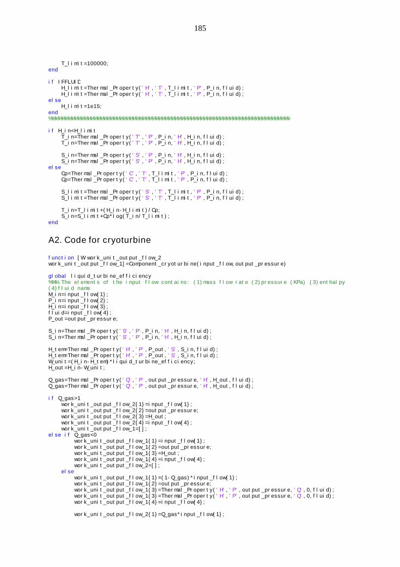
185

T_limit=100000;end

if IFFLUIDH_limit=Thermal_Property('H','T',T_limit,'P',P_in,fluid);H_limit=Thermal_Property('H','T',T_limit,'P',P_in,fluid);

elseH_limit=1e15;

end%%%%%%%%%%%%%%%%%%%%%%%%%%%%%%%%%%%%%%%%%%%%%%%%%%%%%%%%%%%%%%%%%%%%%%%%%%%

if H_in<H_limitT_in=Thermal_Property('T','P',P_in,'H',H_in,fluid);T_in=Thermal_Property('T','P',P_in,'H',H_in,fluid);



S_limit=Thermal_Property('S','T',T_limit,'P',P_in,fluid);S_limit=Thermal_Property('S','T',T_limit,'P',P_in,fluid);

T_in=T_limit+(H_in-H_limit)/Cp;S_in=S_limit+Cp*log(T_in/T_limit);

end

A2. Code for cryoturbine

function [W work_unit_output_flow_2work_unit_output_flow_1]=Component_cryoturbine(input_flow,output_pressure)

global liquid_turbine_efficiency%%% The elements of the input flow contains: (1)mass flow rate (2)pressure (KPa) (3)enthalpy(4)fluid nameM_in=input_flow{1};P_in=input_flow{2};H_in=input_flow{3};fluid=input_flow{4};P_out=output_pressure;


H_tem=Thermal_Property('H','P',P_out,'S',S_in,fluid);H_tem=Thermal_Property('H','P',P_out,'S',S_in,fluid);W_unit=(H_in-H_tem)*liquid_turbine_efficiency;H_out=H_in-W_unit;

Q_gas=Thermal_Property('Q','P',output_pressure,'H',H_out,fluid);Q_gas=Thermal_Property('Q','P',output_pressure,'H',H_out,fluid);

if Q_gas>1work_unit_output_flow_2{1}=input_flow{1};work_unit_output_flow_2{2}=output_pressure;work_unit_output_flow_2{3}=H_out;work_unit_output_flow_2{4}=input_flow{4};work_unit_output_flow_1=[];

else if Q_gas<0work_unit_output_flow_1{1}=input_flow{1};work_unit_output_flow_1{2}=output_pressure;work_unit_output_flow_1{3}=H_out;work_unit_output_flow_1{4}=input_flow{4};work_unit_output_flow_2=[];

elsework_unit_output_flow_1{1}=(1-Q_gas)*input_flow{1};work_unit_output_flow_1{2}=output_pressure;work_unit_output_flow_1{3}=Thermal_Property('H','P',output_pressure,'Q',0,fluid);work_unit_output_flow_1{3}=Thermal_Property('H','P',output_pressure,'Q',0,fluid);work_unit_output_flow_1{4}=input_flow{4};

work_unit_output_flow_2{1}=Q_gas*input_flow{1};

186

work_unit_output_flow_2{2}=output_pressure;T_tem=Thermal_Property('T','P',output_pressure,'Q',1,fluid)+1;T_tem=Thermal_Property('T','P',output_pressure,'Q',1,fluid)+1;work_unit_output_flow_2{3}=Thermal_Property('H','T',T_tem,'P',output_pressure,fluid);work_unit_output_flow_2{3}=Thermal_Property('H','T',T_tem,'P',output_pressure,fluid);work_unit_output_flow_2{4}=input_flow{4};

endend

W=W_unit*M_in;

A3. Code for pump

function [W work_unit_output_flow]=Component_pump(input_flow,output_pressure)

global pump_efficiency

%%% The elements of the input flow contains: (1)mass flow rate (2)pressure (KPa) (3)enthalpy(4)fluid nameHin=input_flow{3};Sin=Thermal_Property('S','P',input_flow{2},'H',input_flow{3},input_flow{4});Sin=Thermal_Property('S','P',input_flow{2},'H',input_flow{3},input_flow{4});Hout_temp=Thermal_Property('H','P',output_pressure,'S',Sin,input_flow{4});Hout_temp=Thermal_Property('H','P',output_pressure,'S',Sin,input_flow{4});W_consuming_unit=(Hin-Hout_temp)/pump_efficiency;Hout=Hin-W_consuming_unit;W=input_flow{1}*W_consuming_unit;

work_unit_output_flow{1}=input_flow{1};work_unit_output_flow{2}=output_pressure;work_unit_output_flow{3}=Hout;work_unit_output_flow{4}=input_flow{4};

A4. Code for throttle valve

function [W work_unit_output_flow_2work_unit_output_flow_1]=Component_throttlevalve(input_flow,output_pressure)

%%% The elements of the input flow contains: (1)mass flow rate (2)pressure (KPa) (3)enthalpy(4)fluid nameM_in=input_flow{1};P_in=input_flow{2};H_in=input_flow{3};fluid=input_flow{4};P_out=output_pressure;

W=0;

Q_gas=Thermal_Property('Q','P',output_pressure,'H',H_in,fluid);Q_gas=Thermal_Property('Q','P',output_pressure,'H',H_in,fluid);

if Q_gas>1work_unit_output_flow_2{1}=input_flow{1};work_unit_output_flow_2{2}=output_pressure;work_unit_output_flow_2{3}=H_in;work_unit_output_flow_2{4}=input_flow{4};work_unit_output_flow_1=[];

else if Q_gas<0work_unit_output_flow_1{1}=input_flow{1};work_unit_output_flow_1{2}=output_pressure;work_unit_output_flow_1{3}=Thermal_Property('H','P',output_pressure,'Q',0,fluid);work_unit_output_flow_1{3}=Thermal_Property('H','P',output_pressure,'Q',0,fluid);work_unit_output_flow_1{4}=input_flow{4};work_unit_output_flow_2=[];

elsework_unit_output_flow_1{1}=(1-Q_gas)*input_flow{1};work_unit_output_flow_1{2}=output_pressure;T_tem=Thermal_Property('T','P',output_pressure,'Q',1,fluid)+1;T_tem=Thermal_Property('T','P',output_pressure,'Q',1,fluid)+1;

187

work_unit_output_flow_2{3}=Thermal_Property('H','T',T_tem,'P',output_pressure,fluid);work_unit_output_flow_2{3}=Thermal_Property('H','T',T_tem,'P',output_pressure,fluid);work_unit_output_flow_1{4}=input_flow{4};

work_unit_output_flow_2{1}=Q_gas*input_flow{1};work_unit_output_flow_2{2}=output_pressure;work_unit_output_flow_2{3}=Thermal_Property('H','P',output_pressure,'Q',1,fluid);work_unit_output_flow_2{3}=Thermal_Property('H','P',output_pressure,'Q',1,fluid);work_unit_output_flow_2{4}=input_flow{4};

endend

A5. Code for turbine

function [W work_unit_output_flow]=Component_turbine(input_flow,output_pressure)

global T_ambientglobal turbine_isentropic_efficiencycalcualtion=0;%%% The elements of the input flow contains: (1)mass flow rate (2)pressure (KPa) (3)enthalpy(4)fluid nameM_in=input_flow{1};P_in=input_flow{2};H_in=input_flow{3};fluid=input_flow{4};P_out=output_pressure;

T_min=T_ambient;



H_tem=Thermal_Property('H','P',P_out,'S',S_in,fluid);H_tem=Thermal_Property('H','P',P_out,'S',S_in,fluid);W_unit=(H_in-H_tem)*turbine_isentropic_efficiency;Hout=H_in-W_unit;W=M_in*W_unit;

work_unit_output_flow{1}=input_flow{1};work_unit_output_flow{2}=output_pressure;if T_in<T_min

work_unit_output_flow{3}=Hout;else

work_unit_output_flow{3}=H_tem;endwork_unit_output_flow{4}=input_flow{4};

if calcualtionT_tem_out=Thermal_Property('T','P',P_out,'S',S_in,fluid);T_tem_out=Thermal_Property('T','P',P_out,'S',S_in,fluid);H_tem_out=Thermal_Property('H','P',P_out,'S',S_in,fluid);H_tem_out=Thermal_Property('H','P',P_out,'S',S_in,fluid);

if T_tem_out>T_minT_out=T_tem_out;W=M_in*(H_in-H_tem_out)*turbine_isentropic_efficiency;H_out=H_tem_out;work_unit_output_flow{1}=input_flow{1};work_unit_output_flow{2}=output_pressure;work_unit_output_flow{3}=H_out;work_unit_output_flow{4}=input_flow{4};

elseT_out=T_min;P_min = P_out;P_max = P_in;

while P_max-P_min > 1x = (P_max+P_min)/2;

188

Tout=Thermal_Property('T','P',x,'S',S_in,fluid);Tout=Thermal_Property('T','P',x,'S',S_in,fluid);

if Tout<T_minP_min = x;

elseP_max = x;

end

end

P_adiabatic=P_min;Hout_temp=Thermal_Property('H','P',P_adiabatic,'S',S_in,fluid);Hout_temp=Thermal_Property('H','P',P_adiabatic,'S',S_in,fluid);W_consuming_adiabatic_unit=(H_in-Hout_temp)*turbine_isentropic_efficiency;

P_compressor_inlet=P_adiabatic;T_compressor_inlet=T_min;P_compressor_outlet=P_out;T_compressor_outlet=T_min;









W_compressor_isothermal_unit=-((H_compressor_outlet-H_compressor_inlet)-T_min*(S_compressor_outlet-S_compressor_inlet))*turbine_isothermal_efficiency;

W=(W_consuming_adiabatic_unit+W_compressor_isothermal_unit)*M_in;work_unit_output_flow{1}=input_flow{1};work_unit_output_flow{2}=output_pressure;work_unit_output_flow{3}=H_compressor_outlet;work_unit_output_flow{4}=input_flow{4};

endend

A6. Code for control parameters

function CONTROL_PARAMETER

%%%%%%%%%%%%%%%%%%%%%%%%%%%%%%%%%%%%%%%%%%%%%%%%%%%%%%%%%%%%%%%%%%%%%%%%%%%%%%%%%%%%%%%%%%%%%%%%% Mode setting %%%%%%%%%%%%%%%%%%%%%%%%%%%%%%%%%%%%%%%%%%%%%%%%%%%%%%%%%%%%%%%%%%%%%%%%%%%%%%%%%%%%%%%%%%%%%%%%%%%%%%%%%%%%%%%%global optimisation_modeoptimisation_mode=0;

%%%%%%%%%%%%%%%%%%%%%%%%%%%%%%%%%%%%%%%%%%%%%%%%%%%%%%%%%%%%%%%%%%%%%%%%%%%%%%%%%%%%%%%%%%%%%%%%% Ambient condition %%%%%%%%%%%%%%%%%%%%%%%%%%%%%%%%%%%%%%%%%%%%%%%%%%%%%%%%%%%%%%%%%%%%%%%%%%%%%%%%%%%%%%%%%%%%%%%%%%%%%%%%%%%global P_ambientglobal T_ambientP_ambient=1.01325e2;T_ambient=298.15;%%%%%%%%%%%%%%%%%%%%%%%%%%%%%%%%%%%%%%%%%%%%%%%%%%%%%%%%%%%%%%%%%%%%%%%%%%%%%%%%%%%%%%%%%%%%%%%% stream splitting %%%%%%%%%%%%%%%%%%%%%%%%%%%%%%%%%%%%%%%%%%%%%%%%%%%%%%%%%%%%%%%%%%%%%%%%%%%%%%%%%%%%%%%%%%%%%%%%%%%%%%%%%%%%%%

189

global min_splitting_coefficienyglobal max_splitting_coefficieny

min_splitting_coefficieny=0.1;max_splitting_coefficieny=0.9; %%if the flow splitting coefficient is too high or too low thanthe splitting should not be taken place.%%ifproduct=1;%%%%%%%set if the liquid is the product%%%%%%%%%%%%%%%%%%%%%%%%%%%%%%%%%%%%%%%%%%%%%%%%%%%%%%%%%%%%%%%%%%%%%%%%%%%%%%%%%%%%%%%%%%%%%% Component efficiency %%%%%%%%%%%%%%%%%%%%%%%%%%%%%%%%%%%%%%%%%%%%%%%%%%%%%%%%%%%%%%%%%%%%%%%%%%%%%%%%%%%%%%%%%%%%%%%%%%%%%%%%%%%%global pump_efficiencyglobal turbine_isentropic_efficiencyglobal turbine_isothermal_efficiencyglobal compressor_isentropic_efficiencyglobal compressor_isothermal_efficiencyglobal liquid_turbine_efficiency

turbine_isentropic_efficiency=0.88;turbine_isothermal_efficiency=0.88;compressor_isentropic_efficiency=0.87;compressor_isothermal_efficiency=0.87;liquid_turbine_efficiency=0.7;pump_efficiency=0.77;%%%%%%%%%%%%%%%%%%%%%%%%%%%%%%%%%%%%%%%%%%%%%%%%%%%%%%%%%%%%%%%%%%%%%%%%%%%%%%%%%%%%%%%%% minimum temperature converge for temperature capture %%%%%%%%%%%%%%%%%%%%%%%%%%%%%%%%%%%%%%%%%%%%%%%%%%%%%%%%%%%%%%%%%%%%%%%%%%%%%%%%%%global minimum_temperature_grid

minimum_temperature_grid=0.1;%%%%%%%%%%%%%%%%%%%%%%%%%%%%%%%%%%%%%%%%%%%%%%%%%%%%%%%%%%%%%%%%%%%%%%%%%%%%%%%%%%%%%%%%%%%% Fluid conditions setting %%%%%%%%%%%%%%%%%%%%%%%%%%%%%%%%%%%%%%%%%%%%%%%%%%%%%%%%%%%%%%%%%%%%%%%%%%%%%%%%%%%%%%%%%%%%%%%%%%%%%%%%%%%global Main_fluidglobal RefrigerantMain_fluid='NITROGEN';Refrigerant='HELIUM';

global Stage_main_flowglobal ifproducr_main_flowglobal Stage_refrigeration

Stage_main_flow=4;ifproducr_main_flow=1;Stage_refrigeration=5;%%%%%%%%%%%%%%%%%%%%%%%%%%%%%%%%%%%%%%%%%%%%%%%%%%%%%%%%%%%%%%%%%%%%%%%%%%%%%%%%%%%%%%%%%%%% Approach temperature %%%%%%%%%%%%%%%%%%%%%%%%%%%%%%%%%%%%%%%%%%%%%%%%%%%%%%%%%%%%%%%%%%%%%%%%%%%%%%%%%%%%%%%%%%%%%%%%%%%%%%%%%%%%%%%global Approach_temperatureglobal min_approach_temperatureApproach_temperature=3;min_approach_temperature=Approach_temperature;%%%%%%%%%%%%%%%%%%%%%%%%%%%%%%%%%%%%%%%%%%%%%%%%%%%%%%%%%%%%%%%%%%%%%%%%%%%%%%%%%%%%%%%%%%% Initial solution setting %%%%%%%%%%%%%%%%%%%%%%%%%%%%%%%%%%%%%%%%%%%%%%%%%%%%%%%%%%%%%%%%%%%%%%%%%%%%%%%%%%%%%%%%%%%%%%%%%%%%%%%%%%%%global Initial_solutionInitial_solution=[253/300 ...

1000/100 273/300 1500/100 273/300 2000/100 90/300 ...2000/100 90/300 2000/100 90/300 2000/100 90/300 ...3000/100 227.5/300 247.5/300 1.0 ...1000/100 84/300 114/300 1.0 ...400/100 84.3/300 114.3/300 1.0 ...150/100 74.4/300 114.4/300 1.0 ...100/100 74/300 95/300 1.0 ...3000/100 273/300 273/300 1.0 ...3000/100 273/300 273/300 1.0 ...3000/100 273/300 273/300 1.0 ...3000/100 273/300 273/300 1.0 ...3000/100 273/300 273/300 1.0 ...3000/100 273/300 273/300 1.0 ...3000/100 273/300 273/300 1.0 ...3000/100 273/300 273/300 1.0 ...3000/100 273/300 273/300 1.0 ...3000/100 273/300 273/300 1.0 ...

190

];%%%%%%%%%%%%%%%%%%%%%%%%%%%%%%%%%%%%%%%%%%%%%%%%%%%%%%%%%%%%%%%%%%%%%%%%%%%%%%%%%%%%%%%%%%% Boundary conditions %%%%%%%%%%%%%%%%%%%%%%%%%%%%%%%%%%%%%%%%%%%%%%%%%%%%%%%%%%%%%%%%%%%%%%%%%%%%%%%%%%%%%%%%%%%%%%%%%%%%%%%%%%%%%%%%%global Number_of_variablesglobal Number_of_variables_mail_flowglobal Number_of_variables_refrigerationglobal Lower_conditionglobal Upper_conditionNumber_of_variables_mail_flow=2*(Stage_main_flow-1);Number_of_variables_refrigeration=2^(Stage_refrigeration-1)-1;Number_of_variables=2*Number_of_variables_mail_flow+4*Number_of_variables_refrigeration+1;%%%% Lower conditionLower_condition(1)=150/300;if Number_of_variables_mail_flow>1

for i=1:(Number_of_variables_mail_flow-1)Lower_condition(2*i)=P_ambient/100;Lower_condition(2*i+1)=90/300;

endendLower_condition(2*Number_of_variables_mail_flow)=500/100;Lower_condition(2*Number_of_variables_mail_flow+1)=80/300;if Number_of_variables_refrigeration>0

for i=1:Number_of_variables_refrigerationLower_condition(4*i-3+2*Number_of_variables_mail_flow+1)=P_ambient/100;Lower_condition(4*i-2+2*Number_of_variables_mail_flow+1)=60/300;Lower_condition(4*i-1+2*Number_of_variables_mail_flow+1)=60/300;Lower_condition(4*i+2*Number_of_variables_mail_flow+1)=0.1;

endend%%%%%%%%%%%%%%%%%%%%%%%%%%%%%%%%%%%%%%%%%%%%%%%%%%%%%%%%%%%%%%%%%%%%%%%%%%%%%%% Upper conditionUpper_condition(1)=280/300;if Number_of_variables_mail_flow>1

for i=1:(Number_of_variables_mail_flow-1)Upper_condition(2*i)=4000/100;Upper_condition(2*i+1)=T_ambient/300;

endendUpper_condition(2*Number_of_variables_mail_flow)=8000/100;Upper_condition(2*Number_of_variables_mail_flow+1)=120/300;if Number_of_variables_refrigeration>0

for i=1:Number_of_variables_refrigerationUpper_condition(4*i-3+2*Number_of_variables_mail_flow+1)=3000/100;Upper_condition(4*i-2+2*Number_of_variables_mail_flow+1)=T_ambient/300;Upper_condition(4*i-1+2*Number_of_variables_mail_flow+1)=T_ambient/300;Upper_condition(4*i+2*Number_of_variables_mail_flow+1)=1.7;

endend

%c=(Lower_condition+Upper_condition)/2;%%%%%%%%%%%%%%%%%%%%%%%%%%%%%%%%%%%%%%%%%%%%%%%%%%%%%%%%%%%%%%%%%%%%%%%%%%%%%%%%%%%%%%%%%%%%%%%% Output setting %%%%%%%%%%%%%%%%%%%%%%%%%%%%%%%%%%%%%%%%%%%%%%%%%%%%%%%%%%%%%%%%%%%%%%%%%%%%%%%%%%%%%%%%%%%%%%%%%%%%%%%%%%%%%%%%%

global Output_Objective_trendglobal Output_Objective_dataglobal Output_EHTF_trendglobal Output_EHTF_dataglobal Output_Optimal_vectorglobal Output_Composite_curvesglobal Output_Captial_costglobal Output_Liuqid_productglobal Output_Heat_flowglobal Output_State_parameter

Output_Objective_trend=1;Output_Objective_data=0;Output_EHTF_trend=1;Output_EHTF_data=0;Output_Optimal_vector=0;Output_Composite_curves=1;Output_Captial_cost=0;Output_Liuqid_product=0;

191

Output_Heat_flow=1;Output_State_parameter=0;

A7. Code for EHTF calcualtion

function EHTF=EHTF_capture(Z1,Z2)

N_plot=0;N_EHTF=0;

EHTF=0;global ifplotglobal T_ambientglobal min_approach_temperature

if ifplotN=200;

elseN=50;

end

approach_temperature=100;A1=length(Z1);A2=length(Z2);A=A1+A2;for i=1:A1

y{i}=Z1{i};a=Z1{i};T_in_1=ST(a{2},a{3},a{5});T_in_2=ST(a{2},a{4},a{5});b={a{1},a{2},T_in_1,T_in_2,a{5}};

end

for i=(A1+1):Ay{i}=Z2{i-A1};a=Z2{i-A1};T_in_1=ST(a{2},a{3},a{5});T_in_2=ST(a{2},a{4},a{5});b={a{1},a{2},T_in_1,T_in_2,a{5}};

end

for i=1:ATempy=y{i};[Q_(i) y_update]= temperature_ordering(y{i});y_update_{i}=y_update;

end

Q_all_HR=0;Q_all_HA=0;

k1=0;k2=0;for i=1:A[Q_all_HR Q_all_HA y_HR y_HA]=heat_source_grouping(Q_all_HR,Q_all_HA,Q_(i),y_update_{i});

if ~isempty(y_HR)k1=k1+1;y_HR_{k1}= y_HR;

end

if ~isempty(y_HA)k2=k2+1;y_HA_{k2}= y_HA;

endend

aaaaa=y_HR_;bbbbb=y_HA_;

if abs((Q_all_HR+Q_all_HA)/Q_all_HR)>0.01approach_temperature=-5;

192

return;else

for i=1:Aapproach_temperature=mass_sign(y{i});if approach_temperature<0

returnend

end

for Q=0:Q_all_HR/N:Q_all_HRif ifplot

N_plot=N_plot+1;Heat_all(N_plot)=Q;Temp_temperature_High(N_plot)=sub_temperature_capture(Q,y_HR_)-273.15;Temp_temperature_Low(N_plot)=sub_temperature_capture(Q,y_HA_)-273.15;

endN_EHTF=N_EHTF+1;Temp_temperature_HR=sub_temperature_capture(Q,y_HR_);Temp_temperature_HA=sub_temperature_capture(Q,y_HA_);Temp_temperature_HR_EHTF(N_EHTF)=sub_temperature_capture(Q,y_HR_);Temp_temperature_HA_EHTF(N_EHTF)=sub_temperature_capture(Q,y_HA_);Approach_temperature_temp=Temp_temperature_HR-Temp_temperature_HA;if Approach_temperature_temp<approach_temperature

approach_temperature=Approach_temperature_temp;if approach_temperature<0

T_high=Temp_temperature_HR;T_low=Temp_temperature_HA;

returnend

endend

end

approach_temperature=approach_temperature;

for i=1:N_EHTFif (1/Temp_temperature_HR_EHTF(i)+1/Temp_temperature_HA_EHTF(i))<2/T_ambient

Temp_temperature_High_temp(i)=Temp_temperature_HR_EHTF(i)-min_approach_temperature;

Temp_temperature_Low_temp(i)=Temp_temperature_HA_EHTF(i);else

Temp_temperature_High_temp(i)=Temp_temperature_HR_EHTF(i);Temp_temperature_Low_temp(i)=Temp_temperature_HA_EHTF(i)+min_approach_temperature;

endend

DD_1=0;DD_2=0;for i=1:(N_EHTF-1)

D_2=1/(Temp_temperature_HA_EHTF(i)+Temp_temperature_HA_EHTF(i+1))-1/(Temp_temperature_HR_EHTF(i)+Temp_temperature_HR_EHTF(i+1));

D_1=1/(Temp_temperature_HA_EHTF(i)+Temp_temperature_HA_EHTF(i+1))-1/(Temp_temperature_HR_EHTF(i)+Temp_temperature_HR_EHTF(i+1))+...

(1/(Temp_temperature_High_temp(i)+Temp_temperature_High_temp(i+1))-1/(Temp_temperature_Low_temp(i)+Temp_temperature_Low_temp(i+1)));

DD_1=DD_1+D_1;DD_2=DD_2+D_2;

end

EHTF=DD_1/DD_2;

function [Q y_update]=temperature_ordering(y2)

if ~isempty(y2)M_1=y2{1};P_1=y2{2};H_1_in=y2{3};H_1_out=y2{4};fluid_1=y2{5};

T_1_in=ST(P_1,H_1_in,fluid_1);T_1_out=ST(P_1,H_1_out,fluid_1);

Q=M_1*(H_1_in-H_1_out);

193

if T_1_in<T_1_outy_update{1}=M_1;y_update{2}=T_1_in;y_update{3}=T_1_out;y_update{4}=P_1;y_update{5}=P_1;y_update{6}=fluid_1;

elsey_update{1}=M_1;y_update{2}=T_1_out;y_update{3}=T_1_in;y_update{4}=P_1;y_update{5}=P_1;y_update{6}=fluid_1;

end

elseQ=[];y_update=y2;

end

function [Q_all_HR Q_all_HA y_HR y_HA]=heat_source_grouping(Q_all_HR,Q_all_HA,Q,y)

if ~isempty(Q)if Q>0

Q_all_HR=Q_all_HR+Q;y_HR=y;y_HA=[];

elseQ_all_HA=Q_all_HA+Q;y_HR=[];y_HA=y;

endelse

y_HR=[];y_HA=[];

end

function T_out=mass_sign(y)

T_out=100;

if ~isempty(y)if y{1}<0

T_out=-5;end

end

%%%%%%%%%%%%%%%%%%%%%%%%%%%%%%%%%%%%%%%%%%%%%%%%%%%%%%%%%%%%%%%%%%%%%%%%%%%%%%%%%%%%%%%%%%%%%%%%%%%%%%%%%%%%%%%%%%%%%%%%%%%%%%%%%%%%%%%%%%%%function T_in=ST(P_in,H_in,fluid)

length_fluid=length(fluid);if length_fluid==3

if fluid=='CO2'IFCO2=1;

elseIFCO2=0;

endelse

IFCO2=0;end%%%%%%%%%%%%%%%%%%%%%%%%%%%%%%%%%%%%%%%%%%%%%%%%%%%%%%%%%%%%%%%%%%%%%%%%%%%

if IFCO2if P_in>100 && P_in<102

if H_in>1.3278e+006Cp=Thermal_Property('C','P',P_in,'H',1.3278e+006,fluid);Cp=Thermal_Property('C','P',P_in,'H',1.3278e+006,fluid);T_in=1050+(H_in-1.3278e+006)/Cp;

elseif H_in>4.3987e+005T_in=Thermal_Property('T','P',P_in,'H',H_in,fluid);T_in=Thermal_Property('T','P',P_in,'H',H_in,fluid);

194

elseif H_in>4.2285e+005Cp=Thermal_Property('C','P',P_in,'H',4.3987e+005,fluid);Cp=Thermal_Property('C','P',P_in,'H',4.3987e+005,fluid);T_in=217+(H_in-4.3987e+005)/Cp;

elseif H_in>-1.5059e+005T_in=195;

elseT_in=195+(H_in+1.5059e+005)/1240;

endelse


end

elseT_in=Thermal_Property('T','P',P_in,'H',H_in,fluid);T_in=Thermal_Property('T','P',P_in,'H',H_in,fluid);

end

A8. Code for initialization

function INITIALIZATION(x)

%%%%%%%%%%%%%%%%%%%%%%%%%%%%%%%%%%%%%%%%%%%%%%%%%%%%%%%%%%%%%%%%%%%%%%%%%%%%%%%%%%%%%%%%%%%% Fluid conditions setting %%%%%%%%%%%%%%%%%%%%%%%%%%%%%%%%%%%%%%%%%%%%%%%%%%%%%%%%%%%%%%%%%%%%%%%%%%%%%%%%%%%%%%%%%%%%%%%%%%%%%%%%%%%global Main_fluidglobal Refrigerantglobal P_ambientglobal T_ambient

global Start_point_main_flowglobal End_point_main_flowglobal Start_point_refrigerationglobal End_point_refrigeration

global Approach_temperature

global Number_of_variables_mail_flowglobal Number_of_variables_refrigeration

H_ambient_main_fluid=Thermal_Property('H','T',T_ambient,'P',P_ambient,Main_fluid);H_ambient_main_fluid=Thermal_Property('H','T',T_ambient,'P',P_ambient,Main_fluid);H_ambient_main_fluid_outlet=Thermal_Property('H','T',T_ambient-2*Approach_temperature,'P',P_ambient,Main_fluid);H_ambient_main_fluid_outlet=Thermal_Property('H','T',T_ambient-2*Approach_temperature,'P',P_ambient,Main_fluid);H_ambient_refrigeration=Thermal_Property('H','T',x(1)*300,'P',P_ambient,Refrigerant);H_ambient_refrigeration=Thermal_Property('H','T',x(1)*300,'P',P_ambient,Refrigerant);Start_point_main_flow={1.0,P_ambient,H_ambient_main_fluid,Main_fluid};End_point_main_flow={P_ambient,H_ambient_main_fluid_outlet,H_ambient_main_fluid_outlet,1};

H_ambient_main_fluid=Thermal_Property('H','T',273,'P',P_ambient,Main_fluid);H_ambient_refrigerant=Thermal_Property('H','T',273,'P',P_ambient,Refrigerant);H_ambient_refrigerant=Thermal_Property('H','T',273,'P',P_ambient,Refrigerant);

Start_point_refrigeration={1.0,P_ambient,H_ambient_refrigeration,Refrigerant};End_point_refrigeration={P_ambient,H_ambient_refrigeration,H_ambient_refrigeration,1};

global outlet_parameter_main_flowglobal outlet_parameter_refrigeration

if Number_of_variables_mail_flow>1for i=1:Number_of_variables_mail_flow

P_tem=x(2*i)*100;H_tem=Thermal_Property('H','T',x(2*i+1)*300,'P',P_tem,Main_fluid);H_tem=Thermal_Property('H','T',x(2*i+1)*300,'P',P_tem,Main_fluid);outlet_parameter_main_flow{i}={P_tem,H_tem};

195

endend

if Number_of_variables_refrigeration>0for i=1:Number_of_variables_refrigeration

P_tem=x(4*i-3+2*Number_of_variables_mail_flow+1)*100;aaaaa=4*i-2+2*Number_of_variables_mail_flow+1;T_tem_1=x(4*i-2+2*Number_of_variables_mail_flow+1)*300;T_tem_2=x(4*i-1+2*Number_of_variables_mail_flow+1)*300;H_tem_1=Thermal_Property('H','T',T_tem_1,'P',P_tem,Refrigerant);H_tem_1=Thermal_Property('H','T',T_tem_1,'P',P_tem,Refrigerant);H_tem_2=Thermal_Property('H','T',T_tem_2,'P',P_tem,Refrigerant);H_tem_2=Thermal_Property('H','T',T_tem_2,'P',P_tem,Refrigerant);if_splitting_or_not=x(4*i+2*Number_of_variables_mail_flow+1);outlet_parameter_refrigeration{i}={P_tem,H_tem_1,H_tem_2,if_splitting_or_not};

endend

A9. Code for main problem setting

function Efficiency_global=MAIN_PROBLEM(x)

global cycle_numberglobal outlet_parameter_main_flowglobal outlet_parameter_refrigeration

global Start_point_main_flowglobal End_point_main_flowglobal Stage_main_flow

global Start_point_refrigerationglobal End_point_refrigerationglobal Stage_refrigeration

global Main_fluid

global Approach_temperature

cycle_number=cycle_number+1;INITIALIZATION(x);

% 1. Please set the Number of the thermal cycle in the form of% 'Number_THERMALCYCLE=2;'.%Number_THERMALCYCLE=2;

% 2. Please set the working fluid for each thermal cycle in the form of% 'Fluid{i}='FLUID';'.%Fluid{1}='NITROGEN';%Fluid{2}='HELIUM';

% 3. Please set if the thermal cycle produce liquid product in the form of% 'If_product{i}=1;' for producing liquid and 'If_product{i}=0;' for no liquid product.If_product{1}=1;If_product{2}=0;

% 4. Please set if the stream split in the thermal cycle in the form of% 'If_split{i}=1;' for yes and 'If_split{i}=0;' for no.%If_split{1}=0;%If_split{2}=1;

% 5. Please set the stages of each thermal cycle in the form of% 'Number_stage{i}=2;'.%Number_stage{1}=3;%Number_stage{2}=4;

% 6. Please set the mass flow rate of each thermal cycle in the form of% 'Mass_flow{i}=1;'.%Mass_flow{1}=1;%Mass_flow{2}=1;

% 7. Please edit the state pressure and temperature of each thermal cycle% in the form of

196

%%%%%%%%%%%%%%%%%%%%%%%%%%%%%%%%%%%%%%%%%%%%%%%%%%%%%%%%%%%%%%%%%%%%%%%%%%%% for i=1:Number_THERMALCYCLE %%%%%% Number_code{i}=1+2^(Number_stage{i}-1); %%%%%% for j=1:Number_code{i} %%%%%% P{j}=[]; %%%%%% T{j}=[]; %%%%%% end %%%%%% Pressure{i}=P; %%%%%% Temperature{i}=T; %%%%%% end %%%%%%%%%%%%%%%%%%%%%%%%%%%%%%%%%%%%%%%%%%%%%%%%%%%%%%%%%%%%%%%%%%%%%%%%%%%%

% 8. Please edit other state parameters of each thermal cycle% in the form of%%%%%%%%%%%%%%%%%%%%%%%%%%%%%%%%%%%%%%%%%%%%%%%%%%%%%%%%%%%%%%%%%%%%%%%%%%%% for i=1:Number_THERMALCYCLE %%%%%% Number_code{i}=1+2^(Number_stage{i}-1); %%%%%% for j=1:Number_code{i} %%%%%% T_split{j}=[]; %%%%%% Q{j}=[]; %%%%%% end %%%%%% Temperature_splitting{i}=T; %%%%%% Coefficient_splitting{i}=Q; %%%%%% end %%%%%%%%%%%%%%%%%%%%%%%%%%%%%%%%%%%%%%%%%%%%%%%%%%%%%%%%%%%%%%%%%%%%%%%%%%%%

% 9. Please edit the objective function% in the below form 'Objective=[];'

[W_main_flow Heat_total_main_flow M_liquid_product_main_flow Output_heat_flow_main_flow]=...

THERMALCYCLE(Start_point_main_flow,End_point_main_flow,Stage_main_flow,If_product{1},outlet_parameter_main_flow);[W_refrigeration Heat_total_refrigeration M_liquid_product_refrigerationOutput_heat_flow_refrigeration]=...

THERMALCYCLE(Start_point_refrigeration,End_point_refrigeration,Stage_refrigeration,If_product{2},outlet_parameter_refrigeration);

Mass_refrigerant=-Start_point_main_flow{1}*Heat_total_main_flow/Heat_total_refrigeration;%%%Mass flow updateStart_point_refrigeration{1}=Mass_refrigerant;[W_refrigeration Heat_total_refrigeration M_liquid_product_refrigerationOutput_heat_flow_refrigeration]=...

THERMALCYCLE(Start_point_refrigeration,End_point_refrigeration,Stage_refrigeration,If_product{2},outlet_parameter_refrigeration);W_total=W_main_flow+W_refrigeration;approach_temperature_real=sub_approach_temperature_capture(Output_heat_flow_main_flow,Output_heat_flow_refrigeration);c=Approach_temperature;if approach_temperature_real<Approach_temperature

Efficiency_global=Approach_temperature-approach_temperature_real;else

Efficiency_global=M_liquid_product_main_flow*Exergy_liquid(Main_fluid)/W_total;

end

function E=Exergy_liquid(Fluid)

global P_ambientglobal T_ambient

H_ambient=Thermal_Property('H','T',T_ambient,'P',P_ambient,Fluid);H_ambient=Thermal_Property('H','T',T_ambient,'P',P_ambient,Fluid);

S_ambient=Thermal_Property('S','T',T_ambient,'P',P_ambient,Fluid);S_ambient=Thermal_Property('S','T',T_ambient,'P',P_ambient,Fluid);

H=Thermal_Property('H','P',P_ambient,'Q',0,Fluid);H=Thermal_Property('H','P',P_ambient,'Q',0,Fluid);

197

S=Thermal_Property('S','P',P_ambient,'Q',0,Fluid);S=Thermal_Property('S','P',P_ambient,'Q',0,Fluid);

E=(H-H_ambient)-T_ambient*(S-S_ambient);

A10. Code for output controling

function [state, options,optchanged] = OUTPUT(options,state,flag)

%global Output_Objective_trendglobal Output_Objective_data%global Output_EHTF_trendglobal Output_EHTF_dataglobal Output_Optimal_vector%global Output_Composite_curves%global Output_Captial_cost%global Output_Liuqid_product%global Output_Heat_flow%global Output_State_parameter

optchanged = false;

switch flagcase 'init'

%disp('Starting the algorithm');case {'iter','interrupt'}

%disp('Iterating ...')[unused,best] = min(state.Score);%a=state.Best;%b=state.Score;%c=state.Expectation;d=state.Population(best,:);[Efficiency_storage EHTF_value]=EHTF_output(d);

if Output_Objective_dataoutput_1=fopen('exergy_efficiency.txt','a');fprintf(output_1,'\n%12.6g', -unused);fclose(output_1);

end

if Output_EHTF_dataoutput_2=fopen('EHTF_value.txt','a');fprintf(output_2,'\n%12.6g', EHTF_value);fclose(output_2);

end

if Output_Optimal_vectoroutput_3=fopen('Detail_vector.txt','a');fprintf(output_3,'\n%E\t %E\t %E\t %E\t %E\t %E\t %E\t %E\t %E\t %E\t %E\t\n',d);fclose(output_3);

end

case 'done'%disp('Performing final task');

end

A11. Code for power transfer process calcuation

function [W work_unit_output_flow_1 work_unit_output_flow_2] =Power_transfer(input_flow,output_pressure)%STREAM_SPLITTING Summary of this function goes here% This function is used to simulate a flow splitting

a=length(input_flow); %% The elements of the input flow contains: (1)mass flow rate(2)pressure (KPa) (3)enthalpy

%%(4)fluid name (5)splitting coefficient (0<x<1)if a<4

error ('incorrect fluid information');end

if ~ischar(input_flow{4})

198

error ('incorrect fluid name');end

%%%%%%%%%%%%%%%%%%%%%%%%%%%%%%%%%%%%%%%%%%%%%%%%%%%%%%%%%%%%%%%%%%%%%%%%%%%%%%%%%%%%%%%%%%%%%%%%%%%%%%%%%%%%%%%%%%%%%%%%%%%%Section 1 %% calculating the powerconsumption%%%%%%%%%%%%%%%%%%%%%%%%%%%%%%%%%%%%%%%%%%%%%%%%%%%%%%%%%%%%%%%%%%%%%%%%%%%%%%%%%%%%%%%%%%%%%%%%%%%%%%%%%%%%%%%%%%%%%%%%%if_throttle_valve=1; %%%%%1 for valve and 0 for liquid turbine

global P_ambient

work_unit_output_flow_2=[];input_pressure=input_flow{2};

input_flow{2};input_flow{3};

D_input_flow=Thermal_Property('D','P',input_flow{2},'H',input_flow{3},input_flow{4});D_input_flow=Thermal_Property('D','P',input_flow{2},'H',input_flow{3},input_flow{4});

D_liquid=Thermal_Property('D','P',P_ambient,'Q',0,input_flow{4});D_liquid=Thermal_Property('D','P',P_ambient,'Q',0,input_flow{4});

if abs(input_pressure-output_pressure)/input_pressure<0.01W=0;for i=1:4work_unit_output_flow_1{i}=input_flow{i};end

else if input_pressure>output_pressure %%Expansion processif D_input_flow<D_liquid*0.3 %% Gas turbine

[W work_unit_output_flow_1]=Component_turbine(input_flow,output_pressure);else if if_throttle_valve%%liquid turbine or throttle valve

[W work_unit_output_flow_1work_unit_output_flow_2]=Component_throttlevalve(input_flow,output_pressure);

else[W work_unit_output_flow_1

work_unit_output_flow_2]=Component_cryoturbine(input_flow,output_pressure);end

endelse %%compression process

if D_input_flow<D_liquid*0.3 %% compressor[W work_unit_output_flow_1]=Component_compressor(input_flow,output_pressure);

else %% pump[W work_unit_output_flow_1]=Component_pump(input_flow,output_pressure);

endend

end

A12. Code for starting the program

function START

global optimisation_modeglobal Initial_solutionglobal Lower_conditionglobal Upper_condition

CONTROL_PARAMETER;LengthofOptimization=length(Lower_condition);optionsold = optimset('display','iter',...'MaxFunEvals',5000,'largescale','on','Diagnostics','on','DiffMaxChange',5e-2,'TolX',1e-2,'TolFun',5e-2,'TolCon',1e-2);options =gaoptimset(optionsold,'InitialPopulation',Initial_solution,'PopulationSize',100,'Generations',200,'OutputFcns',@OUTPUT);if ~optimisation_mode

Efficiency_global=MAIN_PROBLEM(Initial_solution);if Efficiency_global<0

199

disp('Valid solution');Objective=-Efficiency_global

end

else

[initial_vector_liquefaction_opt,fval,exitflag,output]=ga(@MAIN_PROBLEM,LengthofOptimization,[],[],[],[],Lower_condition,Upper_condition,[],options);end

A13. Code for stream structure calcualtion

function [W M_liquid_product heat_flow_1 heat_flow_2 heat_flow_3 heat_flow_4] =stream_splitting(input_flow,output_flow,ifproduct)%STREAM_SPLITTING Summary of this function goes here% This function is used to simulate a flow splitting

global min_splitting_coefficienyglobal max_splitting_coefficieny %%if the flow splitting coefficient is too high or too lowthan the splitting should not be taken place.%%ifproduct=1;%%%%%%%set if the liquid is the productglobal P_ambient

M_liquid_product=0;

a=length(input_flow); %% The elements of the input flow contains: (1)mass flow rate(2)pressure (KPa) (3)enthalpy

%%(4)fluid nameb=length(output_flow);%%(1)output pressure (2)output enthalpy 1 (3)output enthalpy 2(4)splitting coefficient (0<x<1)else

%%no splitting

output_pressure=output_flow{1};output_enthalpy_1=output_flow{2};if b>2

output_enthalpy_2=output_flow{3};else

output_enthalpy_2=0;end

if a<4error ('incorrect fluid information');

end

if ~ischar(input_flow{4})error ('incorrect fluid name');

end

if b>3if output_flow{4}>min_splitting_coefficieny &&

output_flow{4}<max_splitting_coefficienysplitting_or_not=1;%%stream splitting

elsesplitting_or_not=0;

endelse

splitting_or_not=0;end

[W work_unit_output_flow_1 work_unit_output_flow_2] =Power_transfer(input_flow,output_pressure);

if ~isempty(work_unit_output_flow_2)if output_pressure<P_ambient*1.01 && ifproduct

M_liquid_product=work_unit_output_flow_2{1};work_unit_output_flow_2=[];

endend

if ~isempty(work_unit_output_flow_1) && isempty(work_unit_output_flow_2)&& splitting_or_not

200

work_unit_output_flow_1{1}=output_flow{4}*work_unit_output_flow_1{1};work_unit_output_flow_2{1}=(1-output_flow{4})*work_unit_output_flow_1{1};work_unit_output_flow_2{2}=work_unit_output_flow_1{2};work_unit_output_flow_2{3}=work_unit_output_flow_1{3};work_unit_output_flow_2{4}=work_unit_output_flow_1{4};

end

if ~isempty(work_unit_output_flow_2) && isempty(work_unit_output_flow_1)&& splitting_or_notwork_unit_output_flow_1{1}=output_flow{4}*work_unit_output_flow_2{2};work_unit_output_flow_1{2}=work_unit_output_flow_2{2};work_unit_output_flow_1{3}=work_unit_output_flow_2{3};work_unit_output_flow_1{4}=work_unit_output_flow_2{4};work_unit_output_flow_2{1}=(1-output_flow{4})*work_unit_output_flow_2{1};

end

Q_output_flow_1=Thermal_Property('Q','P',output_pressure,'H',output_enthalpy_1,input_flow{4});Q_output_flow_1=Thermal_Property('Q','P',output_pressure,'H',output_enthalpy_1,input_flow{4});Q_output_flow_2=Thermal_Property('Q','P',output_pressure,'H',output_enthalpy_2,input_flow{4});Q_output_flow_2=Thermal_Property('Q','P',output_pressure,'H',output_enthalpy_2,input_flow{4});

if ~isempty(work_unit_output_flow_1)if (Q_output_flow_1>0) && (Q_output_flow_1<1) %%%%%%%%% check if output flow is two

phase flowH_liquid=Thermal_Property('H','P',input_flow{2},'Q',0,input_flow{4})-1000;H_liquid=Thermal_Property('H','P',input_flow{2},'Q',0,input_flow{4})-1000;

H_gas=Thermal_Property('H','P',input_flow{2},'Q',1,input_flow{4})+1000;H_gas=Thermal_Property('H','P',input_flow{2},'Q',1,input_flow{4})+1000;

heat_flow_1{1}=work_unit_output_flow_1{1}*(1-Q_output_flow_1);heat_flow_1{2}=work_unit_output_flow_1{2};heat_flow_1{3}=work_unit_output_flow_1{3};heat_flow_1{4}=H_liquid;heat_flow_1{5}=work_unit_output_flow_1{4};

heat_flow_2{1}=work_unit_output_flow_1{1}*Q_output_flow_1;heat_flow_2{2}=work_unit_output_flow_1{2};heat_flow_2{3}=work_unit_output_flow_1{3};heat_flow_2{4}=H_gas;heat_flow_2{5}=work_unit_output_flow_1{4};

elseheat_flow_1{1}=work_unit_output_flow_1{1};heat_flow_1{2}=work_unit_output_flow_1{2};heat_flow_1{3}=work_unit_output_flow_1{3};heat_flow_1{4}=output_enthalpy_1;heat_flow_1{5}=work_unit_output_flow_1{4};heat_flow_2=[];

endelse

heat_flow_1=[];heat_flow_2=[];

end

if ~isempty(work_unit_output_flow_2)if (Q_output_flow_2>0) && (Q_output_flow_2<1) %%%%%%%%% check if output flow is two

phase flowH_liquid=Thermal_Property('H','P',input_flow{2},'Q',0,input_flow{4})-1000;H_liquid=Thermal_Property('H','P',input_flow{2},'Q',0,input_flow{4})-1000;

H_gas=Thermal_Property('H','P',input_flow{2},'Q',1,input_flow{4})+1000;H_gas=Thermal_Property('H','P',input_flow{2},'Q',1,input_flow{4})+1000;

heat_flow_3{1}=work_unit_output_flow_2{1}*(1-Q_output_flow_2);heat_flow_3{2}=work_unit_output_flow_2{2};heat_flow_3{3}=work_unit_output_flow_2{3};heat_flow_3{4}=H_liquid;heat_flow_3{5}=work_unit_output_flow_2{4};

heat_flow_4{1}=work_unit_output_flow_2{1}*Q_output_flow_2;heat_flow_4{2}=work_unit_output_flow_2{2};heat_flow_4{3}=work_unit_output_flow_2{3};heat_flow_4{4}=H_gas;heat_flow_4{5}=work_unit_output_flow_2{4};

else

201

heat_flow_3{1}=work_unit_output_flow_2{1};heat_flow_3{2}=work_unit_output_flow_2{2};heat_flow_3{3}=work_unit_output_flow_2{3};heat_flow_3{4}=output_enthalpy_2;heat_flow_3{5}=work_unit_output_flow_2{4};heat_flow_4=[];

endelse

heat_flow_3=[];heat_flow_4=[];

end

A14. Code for approach temperature calculation

function approach_temperature=sub_approach_temperature_capture(Z1,Z2)

N_plot=0;

global ifplot

if ifplotN=50;

elseN=50;

end

approach_temperature=100;A1=length(Z1);A2=length(Z2);A=A1+A2;for i=1:A1

y{i}=Z1{i};a=Z1{i};T_in_1=ST(a{2},a{3},a{5});T_in_2=ST(a{2},a{4},a{5});b={a{1},a{2},T_in_1,T_in_2,a{5}};

end

for i=(A1+1):Ay{i}=Z2{i-A1};a=Z2{i-A1};T_in_1=ST(a{2},a{3},a{5});T_in_2=ST(a{2},a{4},a{5});b={a{1},a{2},T_in_1,T_in_2,a{5}};

end

for i=1:ATempy=y{i};[Q_(i) y_update]= temperature_ordering(y{i});y_update_{i}=y_update;

end

Q_all_HR=0;Q_all_HA=0;

k1=0;k2=0;for i=1:A[Q_all_HR Q_all_HA y_HR y_HA]=heat_source_grouping(Q_all_HR,Q_all_HA,Q_(i),y_update_{i});

if ~isempty(y_HR)k1=k1+1;y_HR_{k1}= y_HR;y_HR;

end

if ~isempty(y_HA)k2=k2+1;y_HA_{k2}= y_HA;y_HA;

end

202

end

if abs((Q_all_HR+Q_all_HA)/Q_all_HR)>0.01approach_temperature=-5;return;

elsefor i=1:A

approach_temperature=mass_sign(y{i});if approach_temperature<0

returnend

end

for Q=0:Q_all_HR/N:Q_all_HRif ifplot

N_plot=N_plot+1;Heat_all(N_plot)=Q;Temp_temperature_High(N_plot)=sub_temperature_capture(Q,y_HR_)-273.15*0;Temp_temperature_Low(N_plot)=sub_temperature_capture(Q,y_HA_)-273.15*0;

endTemp_temperature_HR=sub_temperature_capture(Q,y_HR_);Temp_temperature_HA=sub_temperature_capture(Q,y_HA_);Approach_temperature_temp=Temp_temperature_HR-Temp_temperature_HA;if Approach_temperature_temp<approach_temperature

approach_temperature=Approach_temperature_temp;if approach_temperature<0

T_high=Temp_temperature_HR;T_low=Temp_temperature_HA;

returnend

endend

end

if ifplot

plot(Heat_all,Temp_temperature_High,'-.c^',...Heat_all,Temp_temperature_Low,'-.k>','LineWidth',3);

end

approach_temperature=approach_temperature;

function [Q y_update]=temperature_ordering(y2)

if ~isempty(y2)M_1=y2{1};P_1=y2{2};H_1_in=y2{3};H_1_out=y2{4};fluid_1=y2{5};

T_1_in=ST(P_1,H_1_in,fluid_1);T_1_out=ST(P_1,H_1_out,fluid_1);

Q=M_1*(H_1_in-H_1_out);

if T_1_in<T_1_outy_update{1}=M_1;y_update{2}=T_1_in;y_update{3}=T_1_out;y_update{4}=P_1;y_update{5}=P_1;y_update{6}=fluid_1;

elsey_update{1}=M_1;y_update{2}=T_1_out;y_update{3}=T_1_in;y_update{4}=P_1;y_update{5}=P_1;y_update{6}=fluid_1;

end

elseQ=[];

203

y_update=y2;end

function [Q_all_HR Q_all_HA y_HR y_HA]=heat_source_grouping(Q_all_HR,Q_all_HA,Q,y)

if ~isempty(Q)if Q>0

Q_all_HR=Q_all_HR+Q;y_HR=y;y_HA=[];

elseQ_all_HA=Q_all_HA+Q;y_HR=[];y_HA=y;

endelse

y_HR=[];y_HA=[];

end

function T_out=mass_sign(y)

T_out=100;

if ~isempty(y)if y{1}<0

T_out=-5;end

end

%%%%%%%%%%%%%%%%%%%%%%%%%%%%%%%%%%%%%%%%%%%%%%%%%%%%%%%%%%%%%%%%%%%%%%%%%%%%%%%%%%%%%%%%%%%%%%%%%%%%%%%%%%%%%%%%%%%%%%%%%%%%%%%%%%%%%%%%%%%%function T_in=ST(P_in,H_in,fluid)


if fluid=='CO2'IFCO2=1;

elseIFCO2=0;

endelse

IFCO2=0;end

if length_fluid==6if fluid=='OXYGEN'

IFO2=1;else

IFO2=0;end

elseIFO2=0;

end%%%%%%%%%%%%%%%%%%%%%%%%%%%%%%%%%%%%%%%%%%%%%%%%%%%%%%%%%%%%%%%%%%%%%%%%%%%

if IFCO2if P_in>100 && P_in<102


elseif H_in>4.3987e+005T_in=Thermal_Property('T','P',P_in,'H',H_in,fluid);T_in=Thermal_Property('T','P',P_in,'H',H_in,fluid);

elseif H_in>4.2285e+005Cp=Thermal_Property('C','P',P_in,'H',4.3987e+005,fluid);Cp=Thermal_Property('C','P',P_in,'H',4.3987e+005,fluid);T_in=217+(H_in-4.3987e+005)/Cp;

elseif H_in>-1.5059e+005T_in=195;

elseT_in=195+(H_in+1.5059e+005)/1240;

end

204


end

elseif IFO2if P_in>100 && P_in<102



endelse


endelse


end

A15. Code for process temperature capture

function Temp_temperature=sub_temperature_capture(Q,y1)

global minimum_temperature_grid

A1=length(y1);

Q_all=Q;

Tempa=y1{1};T_min=Tempa{2};T_max=Tempa{3};

for i=2:A1[T_min T_max]=max_min_temperature(y1{i},T_min,T_max);end

a=T_min;b=T_max;

while T_max-T_min > minimum_temperature_grid

x = (T_max+T_min)/2;QQ=0;for i=1:A1

QQ=QQ+Enthalpy_capture(y1{i},x);end

if QQ<Q_allT_min = x;

elseT_max = x;

end

endTemp_temperature=(T_min+T_max)/2;

function Enthalpy=Enthalpy_capture(y2,x)

if ~isempty(y2)

M_1=y2{1};T_1_low=y2{2};T_1_high=y2{3};P_1_low=y2{4};

205

P_1_high=y2{5};fluid_1=y2{6};

if x<T_1_low[S_1_temp H_1_temp]=SH(T_1_low,P_1_low,fluid_1);

elseif x<T_1_highP_1_temp=P_1_low+(P_1_high-P_1_low)*(x-T_1_low)/(T_1_high-T_1_low);[S_1_temp H_1_temp]=SH(x,P_1_temp,fluid_1);

else[S_1_temp H_1_temp]=SH(T_1_high,P_1_high,fluid_1);

end

[S_1_low H_1_low]=SH(T_1_low,P_1_low,fluid_1);

Enthalpy=M_1*(H_1_temp-H_1_low);

elseEnthalpy=0;

end

function [T_min T_max]=max_min_temperature(y2,T_min,T_max)

if ~isempty(y2)if y2{2}<T_min

T_min=y2{2};endif y2{3}>T_max

T_max=y2{3};endend

function [T_min T_max]=max_min(y1,y2,y3,y4,y5,y6,y7,y8,y9,y10,y11,y12,y13,y14,y15)

if ~isempty(y1)T_min=y1{2};T_max=y1{3};return

else if ~isempty(y2)T_min=y2{2};T_max=y2{3};return








else if ~isempty(y10)T_min=y10{2};

206

T_max=y10{3};return





elseT_min=y15{2};T_max=y15{3};

endend

endend

endend

endend

endend

endend

endend

%%%%%%%%%%%%%%%%%%%%%%%%%%%%%%%%%%%%%%%%%%%%%%%%%%%%%%%%%%%%%%%%%%%%%%%%%%%%%%%%%%%%%%%%%%%%%%%%%%%%%%%%%%%%%%%%%%%%%%%%%%%%%%%%%%%%%%%%%%%%

function [S_in H_in]=SH(T_in,P_in,fluid)


if fluid=='CO2'IFCO2=1;T_limit=217;

elseIFCO2=0;T_limit=20;

endelse

T_limit=20;IFCO2=0;

end

if length_fluid==6if fluid=='OXYGEN'

IFO2=1;else

IFO2=0;end

elseIFO2=0;

end%%%%%%%%%%%%%%%%%%%%%%%%%%%%%%%%%%%%%%%%%%%%%%%%%%%%%%%%%%%%%%%%%%%%%%%%%%%

if IFCO2if T_in>1050

S_1050=Thermal_Property('S','T',1050,'P',P_in,fluid);S_1050=Thermal_Property('S','T',1050,'P',P_in,fluid);

H_1050=Thermal_Property('H','T',1050,'P',P_in,fluid);H_1050=Thermal_Property('H','T',1050,'P',P_in,fluid);

Cp=Thermal_Property('C','T',1050,'P',P_in,fluid);

207

Cp=Thermal_Property('C','T',1050,'P',P_in,fluid);

S_in=S_1050+Cp*(log(T_in/1050));H_in=H_1050+Cp*(T_in-1050);

elseif T_in>T_limitS_in=Thermal_Property('S','T',T_in,'P',P_in,fluid);S_in=Thermal_Property('S','T',T_in,'P',P_in,fluid);

H_in=Thermal_Property('H','T',T_in,'P',P_in,fluid);H_in=Thermal_Property('H','T',T_in,'P',P_in,fluid);

elseif T_in>195.15Cp=Thermal_Property('C','T',T_limit,'P',P_in,fluid);Cp=Thermal_Property('C','T',T_limit,'P',P_in,fluid);



S_in=S_limit+Cp*(log(T_in/T_limit));H_in=H_limit+Cp*(T_in-T_limit);

elseif T_in>194.85Cp=Thermal_Property('C','T',T_limit,'P',P_in,fluid);Cp=Thermal_Property('C','T',T_limit,'P',P_in,fluid);



S_tem=S_limit+Cp*(log(195.15/T_limit));H_tem=H_limit+Cp*(195.15-T_limit);

C=573000/(195.15-194.85);S_in=S_tem+C*(log(T_in/195.15));H_in=H_tem+C*(T_in-195.15);




S_tem=S_limit+Cp*(log(195.15/T_limit));H_tem=H_limit+Cp*(195.15-T_limit);

C=573000/(195.15-194.85);S_tem_1=S_tem+C*(log(194.85/195.15));H_tem_1=H_tem+C*(194.85-195.15);

C2=1.24*1000;S_in=S_tem_1+C2*(log(T_in/194.85));H_in=H_tem_1+C2*(T_in-194.85);

endelseif IFO2

if T_in<950S_in=Thermal_Property('S','T',T_in,'P',P_in,fluid);S_in=Thermal_Property('S','T',T_in,'P',P_in,fluid);


elseH_0=Thermal_Property('H','T',950,'P',P_in,fluid);H_0=Thermal_Property('H','T',950,'P',P_in,fluid);

S_0=Thermal_Property('S','T',950,'P',P_in,fluid);S_0=Thermal_Property('S','T',950,'P',P_in,fluid);

Cp=Thermal_Property('C','P',P_in,'H',H_0,fluid);

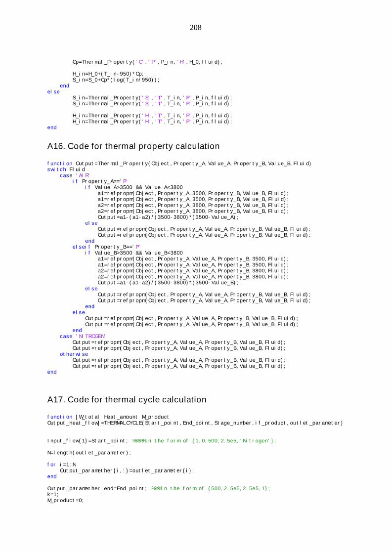
208

Cp=Thermal_Property('C','P',P_in,'H',H_0,fluid);

H_in=H_0+(T_in-950)*Cp;S_in=S_0+Cp*(log(T_in/950));

endelse

S_in=Thermal_Property('S','T',T_in,'P',P_in,fluid);S_in=Thermal_Property('S','T',T_in,'P',P_in,fluid);


end

A16. Code for thermal property calculation

function Output=Thermal_Property(Object,Property_A,Value_A,Property_B,Value_B,Fluid)switch Fluid

case 'AIR'if Property_A=='P'

if Value_A>3500 && Value_A<3800a1=refpropm(Object,Property_A,3500,Property_B,Value_B,Fluid);a1=refpropm(Object,Property_A,3500,Property_B,Value_B,Fluid);a2=refpropm(Object,Property_A,3800,Property_B,Value_B,Fluid);a2=refpropm(Object,Property_A,3800,Property_B,Value_B,Fluid);Output=a1-(a1-a2)/(3500-3800)*(3500-Value_A);

elseOutput=refpropm(Object,Property_A,Value_A,Property_B,Value_B,Fluid);Output=refpropm(Object,Property_A,Value_A,Property_B,Value_B,Fluid);

endelseif Property_B=='P'

if Value_B>3500 && Value_B<3800a1=refpropm(Object,Property_A,Value_A,Property_B,3500,Fluid);a1=refpropm(Object,Property_A,Value_A,Property_B,3500,Fluid);a2=refpropm(Object,Property_A,Value_A,Property_B,3800,Fluid);a2=refpropm(Object,Property_A,Value_A,Property_B,3800,Fluid);Output=a1-(a1-a2)/(3500-3800)*(3500-Value_B);

elseOutput=refpropm(Object,Property_A,Value_A,Property_B,Value_B,Fluid);Output=refpropm(Object,Property_A,Value_A,Property_B,Value_B,Fluid);

endelse

Output=refpropm(Object,Property_A,Value_A,Property_B,Value_B,Fluid);Output=refpropm(Object,Property_A,Value_A,Property_B,Value_B,Fluid);

endcase 'NITROGEN'

Output=refpropm(Object,Property_A,Value_A,Property_B,Value_B,Fluid);Output=refpropm(Object,Property_A,Value_A,Property_B,Value_B,Fluid);

otherwiseOutput=refpropm(Object,Property_A,Value_A,Property_B,Value_B,Fluid);Output=refpropm(Object,Property_A,Value_A,Property_B,Value_B,Fluid);

end

A17. Code for thermal cycle calculation

function [W_total Heat_amount M_productOutput_heat_flow]=THERMALCYCLE(Start_point,End_point,Stage_number,if_product,outlet_parameter)

Input_flow{1}=Start_point; %%%%In the form of {1.0,500,2.5e5,'Nitrogen'};

N=length(outlet_parameter);

for i=1:NOutput_paramether{i,:}=outlet_parameter{i};

end

Output_paramether_end=End_point; %%%In the form of {500,2.5e5,2.5e5,1};k=1;M_product=0;

209

Flow_number_start=1;N=Stage_number;W_total=0;Flow_number_end=1;

Heat_amount=0;

for i=1:Ntem_flow_number=k;for j=Flow_number_start:Flow_number_end

x=i;y=j;if i~=N

[W M_liquid_product heat_flow_1 heat_flow_2 heat_flow_3 heat_flow_4] =stream_splitting(Input_flow{j},Output_paramether{j,:},if_product);

else[W M_liquid_product heat_flow_1 heat_flow_2 heat_flow_3 heat_flow_4] =

stream_splitting(Input_flow{j},Output_paramether_end,if_product);endW_total=W+W_total;M_product=M_product+M_liquid_product;

if ~isempty(heat_flow_1)Output_heat_flow{k,:}=heat_flow_1;Heat_amount=Heat_amount+heat_flow_1{1}*(heat_flow_1{4}-heat_flow_1{3});k=k+1;Input_flow{k}={heat_flow_1{1},heat_flow_1{2},heat_flow_1{4},heat_flow_1{5}};

endif ~isempty(heat_flow_2)

Output_heat_flow{k,:}=heat_flow_2;Heat_amount=Heat_amount+heat_flow_2{1}*(heat_flow_2{4}-heat_flow_2{3});k=k+1;Input_flow{k}={heat_flow_2{1},heat_flow_2{2},heat_flow_2{4},heat_flow_2{5}};





end

endFlow_number_start=tem_flow_number+1;Flow_number_end=k;

end

210

Appendix B Economic Model

The expressions of purchase the main components costs and amortization factor are

presented below.

Cryogenic pumps [176]

71.03540WIP (B1)

Where W is the power consumption of the cryogenic pump (Unit: kW) and PI is the

purchase cost of the cryogenic pump (Unit: USD).

Combustion chamber [176, 205]

4.26018.0exp19728 OCB TmI (B2)

Where m is mass flowrate of air (Unit: kg/s; In the following calculation the mass

flowrate of oxygen and blending gas is used as it is a oxy-combustion process) and

OT is the combustor outlet temperature (Unit: °C). CBI is the purchase cost of the

combustion chamber (Unit: USD).

Compressor [175, 176, 205]

I

O

I

O

CP

CPP

P

P

PmI ln

9.0

75

(B3)

Where m is mass flowrate of the working fluid (Unit: kg/s), CP is the isentropic

efficiency of the compressor, IP and OP are respectively the inlet and outlet

pressures of the compressor and CPI is the purchase cost of the compressor (Unit:

USD).

Expanders (including high pressure turbines and low pressure turbine) [176]:

7.06000WIEP (B4)

Where W is the power output of the expander (Unit: kW) and EPI is the purchase

cost of the expander (Unit: USD).

Gas Turbine [176, 205]

4.26036.0exp1ln92.0

1536

I

O

I

GT

GT TP

PmI

(B5)

211

Where m is mass flowrate of the working fluid (Unit: kg/s), GT is the isentropic

efficiency of the gas turbine, IP and OP are respectively the inlet and outlet

pressures of the gas turbine, IT is the inlet temperature of the gas turbine and GTI is

the purchase cost of the gas turbine (Unit: USD).

Electric generator [176]

95.060WIGEN (B6)

Where W is the generated power of the electric generator (Unit: kW) and GENI is the

purchase cost of the electric generator (Unit: USD).

Counter flow heat exchanger [174]

78.0

093.0130

HX

HX

AI (B7)

Where HXA is the heat exchanger area (Unit: m2) and HXI is the purchase cost of the

counter flow heat exchanger (Unit: USD). HXA is calculated from:

Th

QAHX

(B8)

Where Q is the heat load (Unit: W), h is heat transfer coefficient (Unit: W/(m2·K)) and

T is the average temperature difference between the hot and cold fluids:

Annuity factor [176, 206]

1

1

1

1

1

CP

CP

CPk

CPk

qq

q

qq

qf (B9)

Where k is the amortization period (Unit: year) and CP is the construction period

(Unit: year). q is calculated as:

1001

1001

riinq (B10)

Where in is interest rate (Unit: %/year) and ri is the rate of inflation (Unit: %/year).

212

Appendix C Publications

JOURNAL PAPER:

1)H. Chen, T.N. Cong, W. Yang, C. Tan, Y. Li, and Y. Ding, Progress in electrical

energy storage system: A critical review. Progress in Natural Science 19

(2009) 291-312.

2)Y. Li, H. Chen, and Y. Ding, Fundamentals and applications of cryogen as a

thermal energy carrier: A critical assessment. International Journal of Thermal

Sciences 49 (2010) 941-949.

3)Y. Li, H. Chen, X. Zhang, C. Tan and Y. Ding, Renewable energy carriers:

Hydrogen or liquid air/nitrogen? Applied Thermal Engineering 30 (2010) 1985-

1990.

4)Y. Li, Y. Jin, H. Chen, C. Tan and Y. Ding, An integrated system for thermal

power generation, electrical energy storage and CO2 capture. International

Journal of Energy Research 35 (2011) 1158-1167.

5)H. Chen, Y. Ding, Y. Li, X. Zhang and C. Tan, Air fuelled zero emission road

transportation: A comparative study. Applied Energy 88 (2011) 337-342.

6)Y. Li, X. Wang, Y. Jin and Y. Ding, An integrated solar-cryogen hybrid power

system. Renewable Energy 37 (2012) 76-81.

7)Y. Li and Y. Ding, An optimal design methodology for large-scale gas

liquefaction. Applied Energy, under review.

8)Y. Li, X. Wang and Y. Ding, A cryogen based peak-shaving technology:

systematic approach and techno-economic analysis. International Journal of

Energy Research, accepted.

PATENT:

9)Y. Ding, Y. Li, Y. Jin, H. Chen and C. Tan, An integrated power system for

electricity generation, energy storage and CO2 capture, filed in May 2010,

Chinese Patent.

213

Bibliography

1. Chen H, Cong TN, Yang W, Tan C, Li Y, Ding Y: Progress in electrical energystorage system: A critical review. Progress in Natural Science 2009, 19(3):291-312.

2. Metered half-hourly electricity demands[http://www.nationalgrid.com/uk/Electricity/Data/Demand+Data/]

3. Makansi J, Abboud J: Energy Storage: The missing link in the electricity valuechain. In: Editor|. City|: Publisher|; Year|:Pages|. [|Series Editor (SeriesEditorÊditors|): Series Title|, vol Series Volume|]|.

4. Stodola N, Modi V: Penetration of solar power without storage. Energy Policy2009, 37(11):4730-4736.

5. Kabisama HW: Electrical power engineering: New York ; London : McGraw-Hill;1993.

6. EIA: Electric Power Annual Report. In: Editor|. City|: Publisher|; Year|:Pages|.[|Series Editor (Series EditorÊditors|): Series Title|, vol Series Volume|]|.

7. Hamidi V, Li F, Robinson F: Demand response in the UK's domestic sector.Electric Power Systems Research 2009, 79(12):1722-1726.

8. Ricky Rambharat B, Brockwell AE, Seppi DJ: A threshold autoregressive modelfor wholesale electricity prices. Journal of the Royal Statistical Society: Series C(Applied Statistics) 2005, 54(2):287-299.

9. Veziroglu TN, Sahin S: 21st Century's energy: Hydrogen energy system. EnergyConversion and Management 2008, 49(7):1820-1831.

10. Alnaser WE: Estimation of energy from tide, wave and sea water currents inBahrain. Renewable Energy 1993, 3(2-3):235-238.

11. REN21: Renewables 2007 Global Status Report In: Editor|. City|: Publisher|;Year|:Pages|. [|Series Editor (Series EditorÊditors|): Series Title|, vol SeriesVolume|]|.

12. H.M.Government: Meeting the Energy Challenge: a white paper on energy. In:Editor|. City|: Publisher|; Year|:Pages|. [|Series Editor (Series EditorÊditors|): SeriesTitle|, vol Series Volume|]|.

13. Verbruggen A: Renewable and nuclear power: A common future? Energy Policy2008, 36(11):4036-4047.

14. Weisser D, Garcia RS: Instantaneous wind energy penetration in isolatedelectricity grids: concepts and review. Renewable Energy 2005, 30(8):1299-1308.

15. Meisen P: Linking Renewable Energy Resources Around the World: ACompelling Global Strategy. Power Engineering Review, IEEE 1996, 16(7):18-.

16. Vazquez S, Lukic SM, Galvan E, Franquelo LG, Carrasco JM: Energy StorageSystems for Transport and Grid Applications. Industrial Electronics, IEEETransactions on 2010, 57(12):3881-3895.

17. Walawalkar R, Apt J, Mancini R: Economics of electric energy storage for energyarbitrage and regulation in New York. Energy Policy 2007, 35(4):2558-2568.

18. van der Linden S: Bulk energy storage potential in the USA, currentdevelopments and future prospects. Energy 2006, 31(15):3446-3457.

19. Kondoh J, Ishii I, Yamaguchi H, Murata A, Otani K, Sakuta K, Higuchi N, Sekine S,Kamimoto M: Electrical energy storage systems for energy networks. EnergyConversion and Management 2000, 41(17):1863-1874.

20. Hall PJ, Bain EJ: Energy-storage technologies and electricity generation. EnergyPolicy 2008, 36(12):4352-4355.

214

21. Ibrahim H, Ilinca A, Perron J: Energy storage systems--Characteristics andcomparisons. Renewable and Sustainable Energy Reviews 2008, 12(5):1221-1250.

22. Morisson V, Rady M, Palomo E, Arquis E: Thermal energy storage systems forelectricity production using solar energy direct steam generation technology.Chemical Engineering and Processing: Process Intensification 2008, 47(3):499-507.

23. You Y, Hu EJ: A medium-temperature solar thermal power system and itsefficiency optimisation. Applied Thermal Engineering 2002, 22(4):357-364.

24. Vaivudh S, Rakwichian W, Chindaruksa S: Heat transfer of high thermal energystorage with heat exchanger for solar trough power plant. Energy Conversion andManagement 2008, 49(11):3311-3317.

25. Proceedings of the High efficency integration of thermodynamic solar plant withnatural gas combined cycle: 2007.

26. Smith EM: Storage of electrical energy using supercritical liquid air. ARCHIVE:Proceedings of the Institution of Mechanical Engineers 1847-1982 (vols 1-196) 1977,191(1977):289-298.

27. Kooichi C, Hidefumi A: Evaluation of energy storage method using liquid air.Heat Transfer—Asian Research 2000, 29(5):347-357.

28. Ahern JE: Applications of the 2nd Law of Thermodynamics to Cryogenics - aReview. Energy 1980, 5(8-9):891-897.

29. Hoyeon K: Review on economical efficiency of LNG cold energy use in SouthKorea. In: 23rd World Gas Conference,: 2006; Amsterdam; 2006.

30. Fyke A, Li D, Crane P, Scott DS: Recovery of thermomechanical exergy fromcryofuels. International Journal of Hydrogen Energy 1997, 22(4):435-440.

31. Ordonez CA: Liquid nitrogen fueled, closed Brayton cycle cryogenic heat engine.Energy Conversion and Management 2000, 41(4):331-341.

32. Zalba B, Marín JM, Cabeza LF, Mehling H: Review on thermal energy storage withphase change: materials, heat transfer analysis and applications. Applied ThermalEngineering 2003, 23(3):251-283.

33. Cornot-Gandolphe S, Appert O, Dickel R, Chabrelie M-F, Rojey A: The challengesof turther cost reductions for new supply options (pipeline, LNG, GTL). In: 22ndWorld Gas Conference: 2003; Tokyo, Japan; 2003.

34. Bai FF, Mang ZX: Integration of low-level waste heat recovery and LiquefiedNature Gas cold energy utilization. Chinese Journal of Chemical Engineering 2008,16(1):95-99.

35. Shin JY, Jeon YJ, Maeng DJ, Kim JS, Ro ST: Analysis of the dynamiccharacteristics of a combined-cycle power plant. Energy 2002, 27(12):1085-1098.

36. Saleh B, Koglbauer G, Wendland M, Fischer J: Working fluids for low-temperatureorganic Rankine cycles. Energy 2007, 32(7):1210-1221.

37. Chen Y, Lundqvist P, Johansson A, Platell P: A comparative study of the carbondioxide transcritical power cycle compared with an organic rankine cycle withR123 as working fluid in waste heat recovery. Applied Thermal Engineering 2006,26(17-18):2142-2147.

38. Jha AR: Cryogenic Technology and Applications: Butterworth-Heinemann; 2006.39. Cammarata G, Fichera A, Guglielmino D: Optimization of a liquefaction plant

using genetic algorithms. Applied Energy 2001, 68(1):19-29.40. Maytal BZ: Maximizing production rates of the Linde-Hampson machine.

Cryogenics 2006, 46(1):49-54.41. Mehmet K, Ibrahim D, Marc AR: Performance analysis of gas liquefaction cycles.

International Journal of Energy Research 2008, 32(1):35-43.

215

42. Remeljej CW, Hoadley AFA: An exergy analysis of small-scale liquefied naturalgas (LNG) liquefaction processes. Energy 2006, 31(12):2005-2019.

43. Chang H-M, Chung MJ, Kim MJ, Park SB: Thermodynamic design of methaneliquefaction system based on reversed-Brayton cycle. Cryogenics 2009, 49(6):226-234.

44. Li QY, Ju YL: Design and analysis of liquefaction process for offshore associatedgas resources. Applied Thermal Engineering 2010, In Press, Corrected Proof.

45. Kirillov NG: Analysis of Modern Natural Gas Liquefaction Technologies.Chemical and Petroleum Engineering 2004, 40(7):401-406.

46. Mehmet K, gbreve, lu: Exergy analysis of multistage cascade refrigeration cycleused for natural gas liquefaction. International Journal of Energy Research 2002,26(8):763-774.

47. Brostow AA, Agrawal R, Herron DM, Roberts MJ: Process for nitrogenliquefaction. In. Volume US 6298688 Editor|. City|: Publisher|; Year|:Pages|. [|SeriesEditor (Series Editor^Editors|): Series Title|, vol Series Volume|]|.

48. Chang H-M, Chung MJ, Lee S, Choe KH: An efficient multi-stage Brayton-JTcycle for liquefaction of natural gas. Cryogenics 2010, In Press, Corrected Proof.

49. Finn AJ, Johnson GL, Tomlinson TR: Developments in natural gas liquefaction.Hydrocarbon Processing 1999, 78(4):47-59.

50. Krasae-in S, Stang JH, Neksa P: Development of large-scale hydrogen liquefactionprocesses from 1898 to 2009. International Journal of Hydrogen Energy 2010,35(10):4524-4533.

51. Nogal FD, Kim J-K, Perry S, Smith R: Optimal Design of Mixed RefrigerantCycles. Industrial & Engineering Chemistry Research 2008, 47(22):8724-8740.

52. Li Y, Chen H, Zhang X, Tan C, Ding Y: Renewable energy carriers: Hydrogen orliquid air/nitrogen? Applied Thermal Engineering 2010, 30(14-15):1985-1990.

53. Lee GC, Smith R, Zhu XX: Optimal Synthesis of Mixed-Refrigerant Systems forLow-Temperature Processes. Industrial & Engineering Chemistry Research 2002,41(20):5016-5028.

54. Vaidyaraman S, Maranas CD: Synthesis of Mixed Refrigerant Cascade Cycles.Chemical Engineering Communications 2002, 189(8):1057 - 1078.

55. Mokarizadeh Haghighi Shirazi M, Mowla D: Energy optimization for liquefactionprocess of natural gas in peak shaving plant. Energy 2010, 35(7):2878-2885.

56. Proceedings of the Liquefaction technology; developments through history: 2009.Elsevier.

57. Yooh J-i, Lee H-s, Oh S-t, Lee S-g, Choi K-h: Characteristics of cascade andC3MR cycle on natural gas liquefaction process. World academy of secienceengineering and technology 2009, 59.

58. Jensen JB, Skogestad S, Pantelides WMaC: Optimal operation of a mixed fluidcascade LNG plant. In: Computer Aided Chemical Engineering. Volume Volume 21yEditor|. City|: Publisher|; Year|:Pages|. [|Series Editor (Series Editor^Editors|): SeriesTitle|, vol Series Volume|]|.

59. Miller J, Luyben WL, Blouin S: Economic Incentive for Intermittent Operation ofAir Separation Plants with Variable Power Costs. Industrial & EngineeringChemistry Research 2008, 47(4):1132-1139.

60. Atrey MD: Thermodynamic analysis of Collins helium liquefaction cycle.Cryogenics 1998, 38(12):1199-1206.

216

61. Syed MT, Sherif SA, Veziroglu TN, Sheffield JW: Second law analysis of hydrogenliquefiers operating on the modified Collins cycle. International Journal of EnergyResearch 2001, 25(11):961-978.

62. Kuz'menko IF, Morkovkin IM, Gurov EI: Concept of Building Medium-CapacityHydrogen Liquefiers with Helium Refrigeration Cycle. Chemical and PetroleumEngineering 2004, 40(1):94-98.

63. Proceedings of the Conceptual design of a high efficiency large capacity hydrogenliquefier: 2002; Madison, Wisconsin (USA). AIP.

64. Valenti G, Macchi E: Proposal of an innovative, high-efficiency, large-scalehydrogen liquefier. International Journal of Hydrogen Energy 2008, 33(12):3116-3121.

65. Bracha M, Lorenz G, Patzelt A, Wanner M: Large-scale hydrogen liquefaction inGermany. International Journal of Hydrogen Energy 1994, 19(1):53-59.

66. Nandi TK, Sarangi S: Performance and optimization of hydrogen liquefactioncycles. International Journal of Hydrogen Energy 1993, 18(2):131-139.

67. Yin QS, Li HY, Fan QH, Jia LX: ECONOMIC ANALYSIS OF MIXED-REFRIGERANT CYCLE AND NITROGEN EXPANDER CYCLE IN SMALLSCALE NATURAL GAS LIQUEFIER. AIP Conference Proceedings 2008,985(1):1159-1165.

68. Liquid expanders in LNG liquefaction plants. World Pumps 2002, 2002(431):16-16.

69. Kanoglu M: Cryogenic turbine efficiencies. Exergy, An International Journal 2001,1(3):202-208.

70. Qiang W, Li YZ, Xi C: Exergy analysis of liquefied natural gas cold energyrecovering cycles. International Journal of Energy Research 2005, 29(1):65-78.

71. Bisio G, Tagliafico L: On the recovery of LNG physical exergy. 35th IntersocietyEnergy Conversion Engineering Conference & Exhibit (Iecec), Vols 1 and 2,Technical Papers 2000:309-317.

72. Bisio G, Tagliafico L: On the recovery of LNG physical exergy by means of asimple cycle or a complex system. Exergy, An International Journal 2002, 2(1):34-50.

73. Deng SM, Jin HG, Cai RX, Lin RM: Novel cogeneration power system withliquefied natural gas (LNG) cryogenic exergy utilization. Energy 2004, 29(4):497-512.

74. Qiang W, Li YZ, Jiang W: Analysis of power cycle based on cold energy ofliquefied natural gas and low-grade heat source. Applied Thermal Engineering2004, 24(4):539-548.

75. Szargut J, Szczygiel I: Utilization of the cryogenic exergy of liquid natural gas(LNG) for the production of electricity. Energy 2009, 34(7):827-837.

76. Zhang N, Lior N, Liu M, Han W: COOLCEP (cool clean efficient power): A novelCO2-capturing oxy-fuel power system with LNG (liquefied natural gas) coldnessenergy utilization. Energy 2010, 35(2):1200-1210.

77. Kim TS, Ro ST: Power augmentation of combined cycle power plants using coldenergy of liquefied natural gas. Energy 2000, 25(9):841-856.

78. Kaneko K, Ohtani K, Tsujikawa Y, Fujii S: Utilization of the cryogenic exergy ofLNG by a mirror gas-turbine. Applied Energy 2004, 79(4):355-369.

79. Bisio G, Pisoni C: Thermodynamic analysis of solar energy utilization combinedwith the exploitation of the LNG physical exergy. Journal of Solar EnergyEngineering-Transactions of the Asme 1995, 117(4):333-335.

217

80. Najjar YSH: A Cryogenic Gas-Turbine Engine Using Hydrogen for Waste Heat-Recovery and Regasification of Lng. International Journal of Hydrogen Energy1991, 16(2):129-134.

81. Saxe M, Alvfors P: Advantages of integration with industry for electrolytichydrogen production. Energy 2007, 32(1):42-50.

82. Dispenza C, Dispenza G, La Rocca V, Panno G: Exergy recovery during LNGregasification: Electric energy production - Part one. Applied ThermalEngineering 2008, In Press, Corrected Proof.

83. Dispenza C, Dispenza G, Rocca VL, Panno G: Exergy recovery during LNGregasification: Electric energy production - Part two. Applied ThermalEngineering 2008, In Press, Corrected Proof.

84. Otsuka T: Evolution of an LNG Terminal: Senboku Terminal of Osaka Gas. In:23rd World Gas Conference: 2006; Amsterdam; 2006.

85. Lu T, K.S W: Analysis and optimization of a cascading power cycle with liquefiednatural gas (LNG) cold energy recovery. Applied Thermal Engineering 2008, InPress, Corrected Proof.

86. Miyazaki T, Kang YT, Akisawa A, Kashiwagi T: A combined power cycle usingrefuse incineration and LNG cold energy. Energy 2000, 25(7):639-655.

87. Shi X, Che D: A combined power cycle utilizing low-temperature waste heat andLNG cold energy. Energy Conversion and Management 2009, 50(3):567-575.

88. Hisazumi Y, Yamasaki Y, Sugiyama S: Proposal for a high efficiency LNG power-generation system utilizing waste heat from the combined cycle. Applied Energy1998, 60(3):169-182.

89. Zhang N, Lior N: A novel Brayton cycle with the integration of liquid hydrogencryogenic exergy utilization. Proceedings of the ASME Advanced Energy SystemsDivision 2005, 45:541-551.

90. Zhang N, Lior N: Proposal and analysis of a novel zero CO2 emission cycle withliquid natural gas cryogenic exergy utilization. Journal of Engineering for GasTurbines and Power-Transactions of the Asme 2006, 128(1):81-91.

91. Zhang N, Lior N: A novel near-zero CO2 emission thermal cycle with LNGcryogenic exergy utilization. Energy 2006, 31(10-11):1666-1679.

92. Zhang N, Lior N: A novel Brayton cycle with the integration of liquid hydrogencryogenic exergy utilization. International Journal of Hydrogen Energy 2008,33(1):214-224.

93. Zhang N, Lior N: Two novel oxy-fuel power cycles integrated with natural gasreforming and CO2 capture. Energy 2008, 33(2):340-351.

94. Najjar YSH, Zaamout MS: Cryogenic power conversion with regasification ofLNG in a gas turbine plant. Energy Conversion and Management 1993, 34(4):273-280.

95. Barbir F: Transition to renewable energy systems with hydrogen as an energycarrier. Energy 2009, 34(3):308-312.

96. Salgi G, Donslund B, Alberg Østergaard P: Energy system analysis of utilizinghydrogen as an energy carrier for wind power in the transportation sector inWestern Denmark. Utilities Policy 2008, 16(2):99-106.

97. Wietschel M, Seydel P: Economic impacts of hydrogen as an energy carrier inEuropean countries. International Journal of Hydrogen Energy 2007, 32(15):3201-3211.

98. Pelc R, Fujita RM: Renewable energy from the ocean. Marine Policy 2002,26(6):471-479.

218

99. M.F.Merriam: Wind, waves and tides. Annual Reviews Energy 1978, 3(3):27.100. John T, George S, Margaret M, Pin-Ching M, Ben K, Maria G, J ER, Dan B:

Renewable hydrogen production. International journal of energy research 2008,32(29):379-407.

101. Wurster R, Bent S: Hydrogen and fuel cells, emerging technologies andapplications. International Journal of Hydrogen Energy 2007, 32(18):5109-5110.

102. Holladay JD, Hu J, King DL, Wang Y: An overview of hydrogen productiontechnologies. Catalysis Today 2009, 139(4):244-260.

103. Gardner D: Hydrogen production from renewables. Renewable Energy Focus,9(7):34-37.

104. Granovskii M, Dincer I, Rosen MA: Exergetic life cycle assessment of hydrogenproduction from renewables. Journal of Power Sources 2007, 167(2):461-471.

105. Levene JI, Mann MK, Margolis RM, Milbrandt A: An analysis of hydrogenproduction from renewable electricity sources. Solar Energy 2007, 81(6):773-780.

106. USDE: 'National Hydrogen Energy Roadmap', based on the results of thenational hydrogen roadmap workshop. In: Editor|. City|: Publisher|; Year|:Pages|.[|Series Editor (Series Editor^Editors|): Series Title|, vol Series Volume|]|.

107. Reider R, Edeskuty FJ: Hydrogen safety problems. International Journal ofHydrogen Energy 1979, 4(1):41-45.

108. Solomon BD, Banerjee A: A global survey of hydrogen energy research,development and policy. Energy Policy 2006, 34(7):781-792.

109. Sakintuna B, Lamari-Darkrim F, Hirscher M: Metal hydride materials for solidhydrogen storage: A review. International Journal of Hydrogen Energy 2007,32(9):1121-1140.

110. Hasan MMF, Zheng AM, Karimi IA: Minimizing Boil-Off Losses in LiquefiedNatural Gas Transportation. Industrial & Engineering Chemistry Research 2009,48(21):9571-9580.

111. Lin W, Zhang N, Gu A: LNG (liquefied natural gas): A necessary part in China'sfuture energy infrastructure. Energy 2010, 35(11):4383-4391.

112. Tsujikawa Y, Sawada T: Characteristics of hydrogen-fueled gas turbine cycle withintercooler, hydrogen turbine and hydrogen heater. International Journal ofHydrogen Energy 1985, 10(10):677-683.

113. Najjar YSH: Hydrogen fueled and cooled gas turbine engine. International Journalof Hydrogen Energy 1990, 15(11):827-832.

114. White CM, Steeper RR, Lutz AE: The hydrogen-fueled internal combustion engine:a technical review. International Journal of Hydrogen Energy 2006, 31(10):1292-1305.

115. Jin H, Ishida M: A novel gas turbine cycle with hydrogen-fueled chemical-loopingcombustion. International Journal of Hydrogen Energy 2000, 25(12):1209-1215.

116. Zhang X, Han W, Hong H, Jin H: A chemical intercooling gas turbine cycle withchemical-looping combustion. Energy 2009, 34(12):2131-2136.

117. Cormos C-C: Evaluation of iron based chemical looping for hydrogen andelectricity co-production by gasification process with carbon capture and storage.International Journal of Hydrogen Energy 2010, 35(6):2278-2289.

118. Ishida M, Jin H: A new advanced power-generation system using chemical-looping combustion. Energy 1994, 19(4):415-422.

119. Hotza D, Diniz da Costa JC: Fuel cells development and hydrogen productionfrom renewable resources in Brazil. International Journal of Hydrogen Energy2008, 33(19):4915-4935.

219

120. Dicks AL, Diniz da Costa JC, Simpson A, McLellan B: Fuel cells, hydrogen andenergy supply in Australia. Journal of Power Sources 2004, 131(1-2):1-12.

121. Song C: Fuel processing for low-temperature and high-temperature fuel cells:Challenges, and opportunities for sustainable development in the 21st century.Catalysis Today 2002, 77(1-2):17-49.

122. Bennaceur K, Clark B, Franklin M. Orr J, T.S.Ramakrishnan, Roulet C, Stort E:Hydrogen: A future energy carrier? Oilfield Review 2005.

123. Sharma A, Chen CR, Murty VVS, Shukla A: Solar cooker with latent heat storagesystems: A review. Renewable and Sustainable Energy Reviews, In Press,Corrected Proof.

124. Koca A, Oztop HF, Koyun T, Varol Y: Energy and exergy analysis of a latent heatstorage system with phase change material for a solar collector. RenewableEnergy 2008, 33(4):567-574.

125. Sutthivirode K, Namprakai P, Roonprasang N: A new version of a solar waterheating system coupled with a solar water pump. Applied Energy 2009,86(9):1423-1430.

126. Shukla A, Buddhi D, Sawhney RL: Solar water heaters with phase changematerial thermal energy storage medium: A review. Renewable and SustainableEnergy Reviews 2009, 13(8):2119-2125.

127. Jiang J, Prausnitz JM: Equation of state for thermodynamic properties of chainfluids near-to and far-from the vapor--liquid critical region. The Journal ofChemical Physics 1999, 111(13):5964-5974.

128. Lemmon EW, Huber ML, McLinden MO: NIST Standard Reference Database 23:Reference Fluid Thermodynamic and Transport Properties-REFPROP. In:National Institute of Standards and Technology, Standard Reference Data Program,8.0 edition|. Edited Editor|. City|: Publisher|; Year|:Pages|. [|Series Editor (SeriesEditor^Editors|): Series Title|, vol Series Volume|]|.

129. Pinch technology: basics for the beginners[http://www.cheresources.com/pinchtech3.shtml]

130. Linnhoff B: Thermodynamic analysis in the design of process networks. Ph.D.University of Leeds, Department of Chemical Engineering; 1979.

131. Linnhoff B, Flower JR: Synthesis of heat exchanger networks: I. Systematicgeneration of energy optimal networks. AIChE Journal 1978, 24(4):633-642.

132. Linnhoff B, Mason DR, Wardle I: Understanding heat exchanger networks.Computers & Chemical Engineering 1979, 3(1-4):295-302.

133. Linnhoff B, Flower JR: Synthesis of heat exchanger networks: II. Evolutionarygeneration of networks with various criteria of optimality. AIChE Journal 1978,24(4):642-654.

134. Ebrahim M, Kawari A: Pinch technology: an efficient tool for chemical-plantenergy and capital-cost saving. Applied Energy 2000, 65(1-4):45-49.

135. Kemp IC: Pinch Analysis and Process Integration - A User Guide on ProcessIntegration for the Efficient Use of Energy (2nd Edition). In: Editor|. City|:Publisher|; Year|:Pages|. [|Series Editor (Series Editor^Editors|): Series Title|, volSeries Volume|]|.

136. Aspelund A, Berstad DO, Gundersen T: An Extended Pinch Analysis and Designprocedure utilizing pressure based exergy for subambient cooling. AppliedThermal Engineering 2007, 27(16):2633-2649.

137. Castro P, Matos H, Fernandes MC, Pedro Nunes C: Improvements for mass-exchange networks design. Chemical Engineering Science 1999, 54(11):1649-1665.

220

138. Relvas S, Matos HA, Fernandes MC, Castro P, Nunes CP: AquoMin: A softwaretool for Mass-Exchange Networks targeting and design. Computers & ChemicalEngineering 2008, 32(6):1085-1105.

139. Emhamed AM, Lelkes Z, Rev E, Farkas T, Fonyo Z, Fraser DM: NEW HYBRIDMETHOD FOR MASS EXCHANGE NETWORK OPTIMIZATION. In. Volume194 Editor|. City|: Publisher|; Year|:Pages|. [|Series Editor (Series Editor^Editors|):Series Title|, vol Series Volume|]|.

140. Tan YL, Manan ZA, Foo DCY: Retrofit of Water Network with RegenerationUsing Water Pinch Analysis. Process Safety and Environmental Protection 2007,85(4):305-317.

141. Hallale N: A new graphical targeting method for water minimisation. Advances inEnvironmental Research 2002, 6(3):377-390.

142. Prakash R, Shenoy UV: Targeting and design of water networks for fixed flowrateand fixed contaminant load operations. Chemical Engineering Science 2005,60(1):255-268.

143. Agrawal V, Shenoy UV: Unified conceptual approach to targeting and design ofwater and hydrogen networks. AIChE Journal 2006, 52(3):1071-1082.

144. Fonseca A, Sá V, Bento H, Tavares MLC, Pinto G, Gomes LACN: Hydrogendistribution network optimization: a refinery case study. Journal of CleanerProduction 2008, 16(16):1755-1763.

145. Zhelev TK, Ntlhakana JL: Energy-environment closed-loop through Oxygen Pinch.Computers & Chemical Engineering 1999, 23(Supplement 1):S79-S83.

146. Zhelev TK, Bhaw N: Combined water-oxygen pinch analysis for betterwastewater treatment management. Waste Management 2000, 20(8):665-670.

147. Tantimuratha L, Kokossis AC, Müller FU: The heat exchanger network design as aparadigm of technology integration. Applied Thermal Engineering 2000, 20(15-16):1589-1605.

148. Bogataj M, Bagajewicz MJ: Synthesis of non-isothermal heat integrated waternetworks in chemical processes. Computers & Chemical Engineering 2008,32(12):3130-3142.

149. Mussati SF, Barttfeld M, Aguirre PA, Scenna NJ: A disjunctive programmingmodel for superstructure optimization of power and desalting plants.Desalination 2008, 222(1-3):457-465.

150. Manninen J, Zhu XX: Level-by-level flowsheet synthesis methodology for thermalsystem design. AIChE Journal 2001, 47(1):142-159.

151. Lewin DR, Wang H, Shalev O: A generalized method for HEN synthesis usingstochastic optimization - I. General framework and MER optimal synthesis.Computers & Chemical Engineering 1998, 22(10):1503-1513.

152. Lewin DR: A generalized method for HEN synthesis using stochasticoptimization -- II.: The synthesis of cost-optimal networks. Computers &Chemical Engineering 1998, 22(10):1387-1405.

153. Morton W: Optimization of a heat exchanger network superstructure usingnonlinear programming. Proceedings of the Institution of Mechanical Engineers,Part E: Journal of Process Mechanical Engineering 2002, 216(2):89-104.

154. Chen D, Yang S, Luo X, Wen Q, Ma H: An Explicit Solution for ThermalCalculation and Synthesis of Superstructure Heat Exchanger Networks. ChineseJournal of Chemical Engineering 2007, 15(2):296-301.

221

155. Lotfi R, Boozarjomehry RB: Superstructure Optimization in Heat ExchangerNetwork (HEN) Synthesis Using Modular Simulators and a Genetic AlgorithmFramework. Industrial & Engineering Chemistry Research 2010, 49(10):4731-4737.

156. Mussati SF, Aguirre PA, Scenna NJ: Optimization of alternative structures ofintegrated power and desalination plants. Desalination 2005, 182(1-3):123-129.

157. Futterer E, Gruhn G, Lohe B, Noronha S, Rücker A: Exergy as an objective functionto MINLP problems in process synthesis. Chemical Engineering & Technology1996, 19(3):203-208.

158. Proceedings of the The MATLAB genetic algorithm toolbox: 1995.159. Prakotpol D, Srinophakun T: GAPinch: genetic algorithm toolbox for water pinch

technology. Chemical Engineering and Processing 2004, 43(2):203-217.160. Eurostat: Energy statistics - supply, transformation, consumption. In: Editor|. City|:

Publisher|; Year|:Pages|. [|Series Editor (Series EditorÊditors|): Series Title|, volSeries Volume|]|.

161. Steenhof PA: Decomposition of electricity demand in China's industrial sector.Energy Economics 2006, 28(3):370-384.

162. Lan Y, Bin L, Zongxin W: Present and future power generation in China. NuclearEngineering and Design 2007, 237(12-13):1468-1473.

163. EIA: Electric Power Annual. In: Editor|. City|: Publisher|; Year|:Pages|. [|SeriesEditor (Series EditorÊditors|): Series Title|, vol Series Volume|]|.

164. Division TUNS: Energy Statistics Database. In: Editor|. City|: Publisher|;Year|:Pages|. [|Series Editor (Series EditorÊditors|): Series Title|, vol SeriesVolume|]|.

165. Ashok S: Peak-load management in steel plants. Applied Energy 2006, 83(5):413-424.

166. Larjola J: Electricity from industrial waste heat using high-speed organicRankine cycle (ORC). International Journal of Production Economics 1995, 41(1-3):227-235.

167. Hung TC, Shai TY, Wang SK: A review of organic rankine cycles (ORCs) for therecovery of low-grade waste heat. Energy 1997, 22(7):661-667.

168. Khaliq A, Kumar R, Dincer I: Exergy Analysis of an Industrial Waste HeatRecovery Based Cogeneration Cycle for Combined Production of Power andRefrigeration. In. Volume 131 Editor|. City|: Publisher|; Year|:Pages|. [|Series Editor(Series EditorÊditors|): Series Title|, vol Series Volume|]|.

169. Khaliq A, Kumar R, Dincer I: Performance analysis of an industrial waste heat-based trigeneration system. International Journal of Energy Research 2009,33(8):737-744.

170. Chen H, Goswami DY, Stefanakos EK: A review of thermodynamic cycles andworking fluids for the conversion of low-grade heat. Renewable and SustainableEnergy Reviews 2010, 14(9):3059-3067.

171. Shi XJ, Che DF: Thermodynamic analysis of an LNG fuelled combined cyclepower plant with waste heat recovery and utilization system. InternationalJournal of Energy Research 2007, 31(10):975-998.

172. Pfaff I, Kather A: Comparative thermodynamic analysis and integration issues ofCCS steam power plants based on oxy-combustion with cryogenic or membranebased air separation. Energy Procedia 2009, 1(1):495-502.

173. Kerry FG: Industrial gas handbook: gas separation and purification. Boca Raton:CRC Press; 2007.

222

174. Cheddie DF, Murray R: Thermo-economic modeling of an indirectly coupled solidoxide fuel cell/gas turbine hybrid power plant. Journal of Power Sources 2010,195(24):8134-8140.

175. Sayyaadi H, Babaelahi M: Thermoeconomic optimization of a cryogenicrefrigeration cycle for re-liquefaction of the LNG boil-off gas. InternationalJournal of Refrigeration 2010, 33(6):1197-1207.

176. Silveira JL, Tuna CE: Thermoeconomic analysis method for optimization ofcombined heat and power systems. Part I. Progress in Energy and CombustionScience 2003, 29(6):479-485.

177. Lazzaretto A, Macor A: Direct Calculation of Average and Marginal Costs Fromthe Productive Structure of an Energy System. Journal of Energy Resourse andTechnology 1995, 117(3):171-178.

178. De Lima AC, Guimaraes SC, Camacho JR, Bispo D: Electric energy demandanalysis using fuzzy decision-making system. Melecon 2004: Proceedings of the12th Ieee Mediterranean Electrotechnical Conference, Vols 1-3 2004:811-814.

179. Rabl A, Norford LK: Peak load reduction by preconditioning buildings at night.International Journal of Energy Research 1991, 15(9):781-798.

180. Graus W, Worrell E: Trend in efficiency and capacity of fossil power generation inthe EU. Energy Policy 2009, 37(6):2147-2160.

181. Denton MJ, Rassenti SJ, Smith VL, Backerman SR: Market power in a deregulatedelectrical industry. Decision Support Systems 2001, 30(3):357-381.

182. Harumi W, Koichi C, Osamu Y: Cold heat reused air liquefaction/vaporizationand storage gas turbine electric power system. In: United States Patent. Volume US6,920,795 B2 Editor|. City|: Publisher|; Year|:Pages|. [|Series Editor (SeriesEditorÊditors|): Series Title|, vol Series Volume|]|.

183. Vandor D: System and method for liquid air production, power storage andpower release. In. Volume US 8,020,404,B2 Editor|. City|: Publisher|; Year|:Pages|.[|Series Editor (Series EditorÊditors|): Series Title|, vol Series Volume|]|.

184. Davison J: Performance and costs of power plants with capture and storage ofCO2. Energy 2007, 32(7):1163-1176.

185. Yang H, Xu Z, Fan M, Gupta R, Slimane RB, Bland AE, Wright I: Progress incarbon dioxide separation and capture: A review. Journal of EnvironmentalSciences 2008, 20(1):14-27.

186. Geoffrey PH, Serge SOA: Thermodynamic and related analysis of natural gascombined cycle power plants with and without carbon sequestration.International Journal of Energy Research 2007, 31(12):1180-1201.

187. Pyong Sik P, Young Duk L, Kook Young A: Characteristic evaluation of a CO2-capturing repowering system based on oxy-fuel combustion and exergetic flowanalyses for improving efficiency. International Journal of Energy Research2010:In press.

188. Chen H, Ding Y, Peters T, Berger F: A method of storing energy and a cryogenicenergy storage system. In. Volume PCT/GB2007/000667 Editor|. City|: Publisher|;Year|:Pages|. [|Series Editor (Series EditorÊditors|): Series Title|, vol SeriesVolume|]|.

189. Castle WF: Air separation and liquefaction: recent developments and prospectsfor the beginning of the new millennium. International Journal of Refrigeration2002, 25(1):158-172.

223

190. Weisberg AH, Aceves SM, Espinosa-Loza F, Ledesma-Orozco E, Myers B: Deliveryof cold hydrogen in glass fiber composite pressure vessels. International Journal ofHydrogen Energy 2009, 34(24):9773-9780.

191. Richard; D, A. G, M. C, Jean-Pierre T, Nicolas P: Air separation Unit: Flexibility &Energy Storage. In: 2nd Oxyfuel Combustion Conference: 2011; Queensland,Australia; 2011.

192. K Hossain A, Badr O: Prospects of renewable energy utilisation for electricitygeneration in Bangladesh. Renewable and Sustainable Energy Reviews 2007,11(8):1617-1649.

193. Lior N: Energy resources and use: The present (2008) situation and possiblesustainable paths to the future. Energy 2010, 35(6):2631-2638.

194. Proceedings of the Solar Power – Photovoltaics or Solar Thermal Power Plants?:2001; Brussels.

195. Zhai XQ, Wang RZ: Experimental investigation and performance analysis on asolar adsorption cooling system with/without heat storage. Applied Energy 2010,87(3):824-835.

196. García-Rodríguez L, Blanco-Gálvez J: Solar-heated Rankine cycles for water andelectricity production: POWERSOL project. Desalination 2007, 212(1-3):311-318.

197. Horn M, Führing H, Rheinländer J: Economic analysis of integrated solarcombined cycle power plants: A sample case: The economic feasibility of anISCCS power plant in Egypt. Energy 2003, 29(5-6):935-945.

198. Michael F, Borislav B: High temperature metal hydrides as heat storage materialsfor solar and related applications. International Journal of Molecular Sciences2009(10):325-344.

199. Winter CJ, Sizmann RL, Vant-Hull LL: Solar power plants: Fundamentals,technology, systems economics. Berlin: Springer-Verlag; 1991.

200. Li Y, Chen H, Ding Y: Fundamentals and applications of cryogen as a thermalenergy carrier: A critical assessment. International Journal of Thermal Sciences2010, 49(6):941-949.

201. Chen H, Ding Y: An Overview of Air Liquefaction and Separation Process. In:Editor|. City|: Publisher|; Year|:Pages|. [|Series Editor (Series Editor^Editors|): SeriesTitle|, vol Series Volume|]|.

202. Srinophakun T, Laowithayangkul S, Ishida M: Simulation of power cycle withenergy utilization diagram. Energy Conversion and Management 2001,42(12):1437-1456.

203. Fernández-García A, Zarza E, Valenzuela L, Pérez M: Parabolic-trough solarcollectors and their applications. Renewable and Sustainable Energy Reviews,14(7):1695-1721.

204. Berstad DO, Stang JH, Nekså P: Comparison criteria for large-scale hydrogenliquefaction processes. International Journal of Hydrogen Energy 2009, 34(3):1560-1568.

205. Gorji-Bandpy M, Goodarzian H, Biglari M: The Cost-effective Analysis of a GasTurbine Power Plant. Energy Sources, Part B: Economics, Planning, and Policy2011, 5(4):348-358.

206. Nelson DB, Nehrir MH, Wang C: Unit sizing and cost analysis of stand-alonehybrid wind/PV/fuel cell power generation systems. Renewable Energy 2006,31(10):1641-1656.

Cryogen Based Energy Storage: Process Modelling and ...

Documents

Transcript of Cryogen Based Energy Storage: Process Modelling and ...