Data Driven Modelling of Turbulent Flows using Artificial Neural Networks

BY

LUCA LAMBERTIM.S., Politecnico di Torino, Turin, Italy, 2019

THESIS

Submitted as partial fulfillment of the requirementsfor the degree of Master of Science in Mechanical Engineering

in the Graduate College of theUniversity of Illinois at Chicago, 2020

Chicago, Illinois

Defense Committee:

Roberto Paoli, Chair and Advisor

Suresh Aggarwal

Alessandro Ferrari, Politecnico di Torino

Marco Carlo Masoero, Politecnico di Torino

ACKNOWLEDGMENTS

I would like to express special appreciation to Professor Roberto Paoli, who constantly

proved to be exceptionally kind and available towards me, weekly keeping up-to-date and sug-

gesting new solutions for the thesis work.

My thankfulness extends to Professor Alessandro Ferrari, whose dedication and accentuated

curiosity towards research and innovation encouraged hard work.

Furthermore, I wish to thank my girlfriend Isabella, who constantly stood by me in all

difficult moments during these five years and during the thesis development.

Finally, I wish to express deep gratitude to my family, my father Lucio, my mother Elvira

and sister Chiara, who in innumerable occasions in the last five years supported my commitment

and hopes.

LL

ii

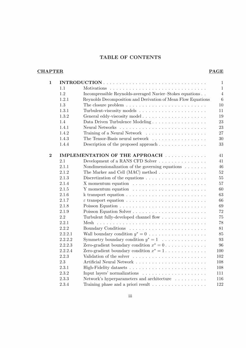
TABLE OF CONTENTS

CHAPTER PAGE

1 INTRODUCTION . . . . . . . . . . . . . . . . . . . . . . . . . . . . . . . . 11.1 Motivations . . . . . . . . . . . . . . . . . . . . . . . . . . . . . . 11.2 Incompressible Reynolds-averaged Navier–Stokes equations . . 41.2.1 Reynolds Decomposition and Derivation of Mean Flow Equations 61.3 The closure problem . . . . . . . . . . . . . . . . . . . . . . . . . 101.3.1 Turbulent-viscosity models . . . . . . . . . . . . . . . . . . . . . 111.3.2 General eddy-viscosity model . . . . . . . . . . . . . . . . . . . . 191.4 Data Driven Turbulence Modeling . . . . . . . . . . . . . . . . . 231.4.1 Neural Networks . . . . . . . . . . . . . . . . . . . . . . . . . . . 231.4.2 Training of a Neural Network . . . . . . . . . . . . . . . . . . . 271.4.3 The Tensor-Basis neural network . . . . . . . . . . . . . . . . . 301.4.4 Description of the proposed approach . . . . . . . . . . . . . . . 33

2 IMPLEMENTATION OF THE APPROACH . . . . . . . . . . . . . 412.1 Development of a RANS CFD Solver . . . . . . . . . . . . . . . 412.1.1 Nondimensionalization of the governing equations . . . . . . . 462.1.2 The Marker and Cell (MAC) method . . . . . . . . . . . . . . . 522.1.3 Discretization of the equations . . . . . . . . . . . . . . . . . . . 552.1.4 X momentum equation . . . . . . . . . . . . . . . . . . . . . . . 572.1.5 Y momentum equation . . . . . . . . . . . . . . . . . . . . . . . 602.1.6 k transport equation . . . . . . . . . . . . . . . . . . . . . . . . . 632.1.7 ε transport equation . . . . . . . . . . . . . . . . . . . . . . . . . 662.1.8 Poisson Equation . . . . . . . . . . . . . . . . . . . . . . . . . . . 692.1.9 Poisson Equation Solver . . . . . . . . . . . . . . . . . . . . . . . 722.2 Turbulent fully-developed channel flow . . . . . . . . . . . . . . 752.2.1 Mesh . . . . . . . . . . . . . . . . . . . . . . . . . . . . . . . . . . 782.2.2 Boundary Conditions . . . . . . . . . . . . . . . . . . . . . . . . 812.2.2.1 Wall boundary condition y∗ = 0 . . . . . . . . . . . . . . . . . . 852.2.2.2 Symmetry boundary condition y∗ = 1 . . . . . . . . . . . . . . 932.2.2.3 Zero-gradient boundary condition x∗ = 0 . . . . . . . . . . . . . 962.2.2.4 Zero-gradient boundary condition x∗ = 1 . . . . . . . . . . . . . 1002.2.3 Validation of the solver . . . . . . . . . . . . . . . . . . . . . . . 1022.3 Artificial Neural Network . . . . . . . . . . . . . . . . . . . . . . 1082.3.1 High-Fidelity datasets . . . . . . . . . . . . . . . . . . . . . . . . 1082.3.2 Input layers’ normalizations . . . . . . . . . . . . . . . . . . . . 1112.3.3 Network’s hyperparameters and architecture . . . . . . . . . . 1162.3.4 Training phase and a priori result . . . . . . . . . . . . . . . . . 122

iii

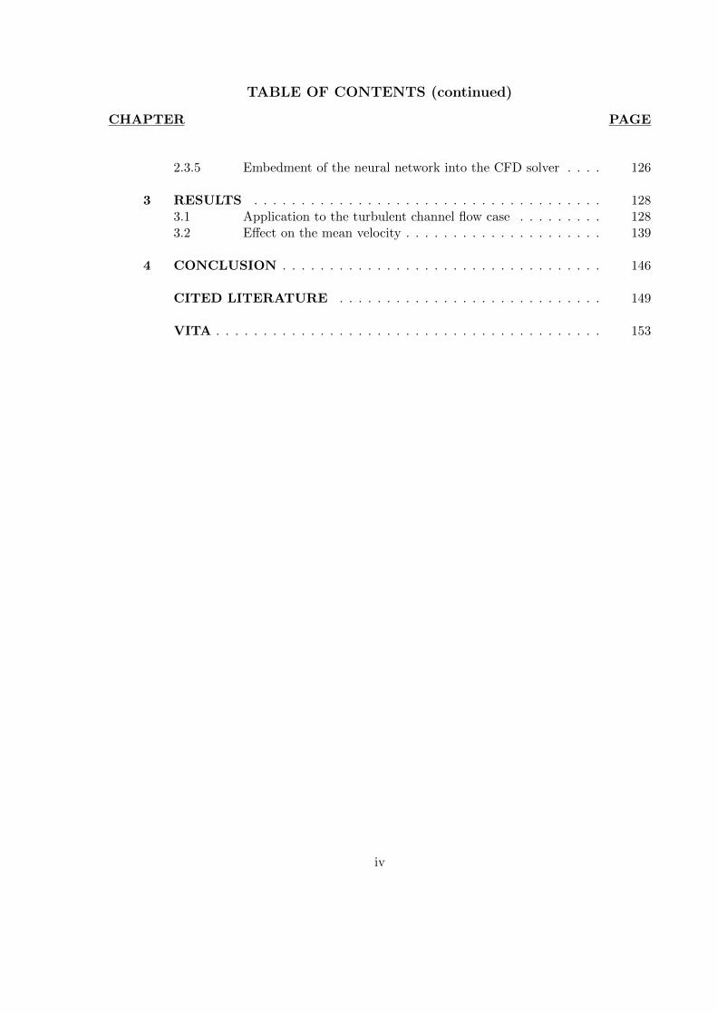
TABLE OF CONTENTS (continued)

CHAPTER PAGE

2.3.5 Embedment of the neural network into the CFD solver . . . . 126

3 RESULTS . . . . . . . . . . . . . . . . . . . . . . . . . . . . . . . . . . . . . 1283.1 Application to the turbulent channel flow case . . . . . . . . . 1283.2 Effect on the mean velocity . . . . . . . . . . . . . . . . . . . . . 139

4 CONCLUSION . . . . . . . . . . . . . . . . . . . . . . . . . . . . . . . . . . 146

CITED LITERATURE . . . . . . . . . . . . . . . . . . . . . . . . . . . . 149

VITA . . . . . . . . . . . . . . . . . . . . . . . . . . . . . . . . . . . . . . . . . 153

iv

LIST OF TABLES

TABLE PAGEI NEURAL NETWORKS’ KEY TERMINOLOGY . . . . . . . . . . 109II TRAINING AND VALIDATION DATASET . . . . . . . . . . . . . 110III NEURAL NETWORK’S ARCHITECTURE . . . . . . . . . . . . . 120IV MODEL’S CHARACTERISTICS . . . . . . . . . . . . . . . . . . . 122

v

LIST OF FIGURES

FIGURE PAGE1 Fully-connected feed-forward network with two hidden layers . . . . 242 Schematic of the TBNN architecture . . . . . . . . . . . . . . . . . . . 323 Comparison of a standard RANS solver with the proposed approach 394 Standard data driven modelling approach (a) vs proposed one (b) . 405 Structured meshes . . . . . . . . . . . . . . . . . . . . . . . . . . . . . . 426 Grid resolutions for wall-functions and near-wall modeling approaches 457 Staggered Arrangement . . . . . . . . . . . . . . . . . . . . . . . . . . . 548 Centered approximation of the first derivative . . . . . . . . . . . . . 569 Control volume for the x-momentum equation . . . . . . . . . . . . . 5710 Control volume for the y-momentum equation . . . . . . . . . . . . . 6011 Control volume for the k-transport equation . . . . . . . . . . . . . . 6312 Control volume for the ε-transport equation . . . . . . . . . . . . . . 6613 Control volume for the continuity equation . . . . . . . . . . . . . . . 6914 Geometry of the channel flow . . . . . . . . . . . . . . . . . . . . . . . 7615 Mesh for the turbulent channel flow . . . . . . . . . . . . . . . . . . . 7816 Near-wall resolution of the mesh for the turbulent channel flow . . . 7917 Channel flow boundary conditions . . . . . . . . . . . . . . . . . . . . 8218 Ghost cells . . . . . . . . . . . . . . . . . . . . . . . . . . . . . . . . . . 8519 Ghost cells for bottom wall boundary condition . . . . . . . . . . . . 8920 Ghost cells for top symmetry boundary condition . . . . . . . . . . . 9521 Ghost cells for left zero-gradient boundary condition . . . . . . . . . 9922 Ghost cells for left zero-gradient boundary condition . . . . . . . . . 10123 Solver validation: Channel flow u+(y+) profile . . . . . . . . . . . . . 10424 Solver validation: Channel flow u+(y/δ) profile . . . . . . . . . . . . 10525 Solver validation: Channel flow k+(y+) and 〈uv(y+) profiles . . . . 10626 Solver validation: von Karman constant . . . . . . . . . . . . . . . . . 10727 Train and validation RMSE . . . . . . . . . . . . . . . . . . . . . . . . 12328 Prediction of Reynolds stress anisotropy tensor on the Duct Flow case 12529 Embedment of the neural network into the CFD solver . . . . . . . . 12730 Turbulent Channel Flow: Reynolds stresses profiles with LEVM . . 13031 Turbulent Channel Flow: DNS Reynolds stresses profiles . . . . . . . 13132 Turbulent Channel Flow: Reynolds Stresses profiles comparison . . . 13333 Turbulent Channel Flow: TBNN Reynolds stresses profiles . . . . . . 13434 Coefficient g(1) predicted by TBNN at first solver iteration . . . . . . 13635 Coefficients g(n) predicted by TBNN at first solver iteration . . . . . 13736 Mean velocity field resulting from enforcing true DNS anisotropy tensor 14137 Mean velocity field resulting from the TBNN approach . . . . . . . . 14238 Turbulent Channel Flow: TBNN 〈uv〉 predicted profile . . . . . . . . 144

vi

LIST OF ABBREVIATIONS

CFD Computational Fluid Dynamics

RANS Reynolds-averaged Navier–Stokes

LES Large Eddy Simulation

DNS Direct Numerical Simulation

SA Spalart-Allmaras

SST Menter Shear Stress Transport

ANN Artificial Neural Network

MLP Multi-layer perceptron

TBNN Tensor Basis Neural Network

SGD Stochastic Gradient Descent

TKE Turbulent kinetic energy

LEVM Linear Eddy Viscosity Model

FVM Finite Volume Method

FEM Finite Elements Method

vii

SUMMARY

Numerical simulations based on Reynolds-averaged Navier Stokes (RANS) models are still

the work-horse tool in engineering design involving turbulent flows [1].

Two decades ago, when LES methods began gaining popularity due to the increase of

computational resources available, it was widely expected to gradually replace the role of RANS

simulations in industrial CFD applications. Over the past two decades, however, while LES-

based methods gained widespread applications, the predicted time of this transition has been

significantly delayed. [2]. In particular, most industrial users are probably decades away from

any routine use of LES or DNS, not to mention the cost, time and user skill it takes to run

these computations [3].

In brief, RANS solvers, particularly those based on standard eddy viscosity models (e.g

k-ε, k-ω, S-A and k-ω SST) are expected to remain the workhorse in industrial CFD of high

Reynolds number flows for decades [2]. Yet,the results of RANS simulations are known to have

large discrepancies in many flows of engineering relevance, particularly those involving swirl,

pressure gradients, or mean streamline curvature. It is common consensus that main reason for

such discrepancies has to be found in the RANS-modeled Reynolds stresses [1].

Due to the the long stagnation in traditional turbulence modeling, researchers began looking

at machine learning as an alternative to improve RANS modeling by leveraging data from high-

fidelity simulations[1]. The objective is to make use of vast amounts of turbulent flows data,

viii

SUMMARY (continued)

machine learning techniques and current understanding of turbulence physics to develop models

with better predictive capabilities in the context of RANS [4].

In a seminar work, Ling et al (2016) developed a neural network architecture capable of

embedding invariance properties into the Reynolds stress tensor predicted in output. Such a

network, named the tensor basis neural network (TBNN), was applied to a variety of flow fields

with encouraging results compared to both classical turbulence models and neural networks

that do not preserve Galilean invariance [5]. Yet, as in most data driven turbulence modelling

approaches, the TBNN was used as a post-processing tool to correct the Reynolds stress tensor

field predicted by a RANS simulation run with standard closure models. This means that,

theoretically, the network can be applied only to correct the Reynolds stress tensor for the

same RANS model on which it has been trained since, in general, different turbulence models

yield different results depending on the flow type. Moreover, there is no physisical insight

that suggests a relation between the RANS velocity gradients - used as inputs of the machine

learning model - and the true Reynolds stress tensor.

Differently, in this work a network with a similar architecture to the Ling’s one was be

trained and tested on a database of high-fidelity data of eight different flows to learn a functional

mapping between the inputs of Pope’s General Eddy Viscosity Model and the anisotropic part

of the Reynolds stress tensor. Then the network was embedded into a CFD RANS solver as

a replacement of the standard closure model - and therefore called at every solver’s iteration.

Lasty, the RANS solver with embedded TBNN was be tested on a canonical flow case - turbulent

channel flow - to evaluate its performances.

ix

SUMMARY (continued)

As for the organization of this work: in Chapter 1 further details on the data driven tur-

bulence modelling will be given, RANS models and equations will be introduced and also an

introduction to Neural Networks will be presented. In Chapter 2, it will be given a detailed

explanation of the RANS CFD solver and the neural network’s implementation. In Chapter 3,

the method will be tested on a turbulent channel flow case and the results will be discussed.

Lastly, in Chapter 4, some meaningful conclusions will be drawn.

x

CHAPTER 1

INTRODUCTION

1.1 Motivations

Turbulence is a common physical characteristic of many industrial fluid flows. For example,

in wind turbine design, the knowledge of turbulent quantities in the incoming flow and in the

blade boundary layers is important for performance. In internal combustion engines, vigorous

turbulence increases fuel/air mixing, thus improving overall efficiency and reducing emissions.

In airplane design, delaying the occurrence of turbulence in boundary layers over the wing

surfaces leads to reduced fuel consumption [6].

These examples, and a vast number of other applications, demonstrate the importance of

determining the effect of turbulence on the performance of engineering devices and justify the

continuous interest in developing more accurate techniques to simulate and predict turbulent

flows[6].

Nowadays, two techniques are at the industry’s computational power’s reach for the numeri-

cal simulation of turbulence flows: RANS (Reynolds Averaged Naviers Stokes) Simulations and

LES (Large Eddy Simulations). DNS use (Direct Numerical Simulations), despite proving to

be the most accurate method for all turbulent flows’ simulation, is still limited to research pur-

poses and canonical flows’ applications, since the computational power required is well beyond

industry capabilities [7].

1

2

Two decades ago, when LES started gaining popularity thanks to the increasing availability

of computational resources, it was widely expected that it would have gradually replaced RANS

methods in industrial CFD for decades to come. In the past two decades, however, while LES-

based methods such as wall-modeled LES and hybrid LES/RANS methods gained widespread

applications and the earlier hope did not diminish, the predicted time when LES would replace

RANS has been significantly delayed[1].

It is under these premises that, in July 2017, a three day Turbulence Modeling Symposium

sponsored by the University of Michigan and NASA, was held in Ann Arbor,Michigan [3]. The

meeting gathered nearly 90 experts from academia, government and industry in order to discuss

the state of the art in turbulence modeling and to wrestle with questions surrounding its future.

One message came through very clearly from the participants of the symposium: industry still

need RANS, all the time[3].

Most industrial users are probably decades away from any routine use of scale resolving

simulations, not to mention the cost, time and user skill it take to run these computations

[3]. In brief, RANS solvers, particularly those based on standard eddy viscosity models (e.g

k-ε, k-ω, S-A and k-ω SST) are expected to remain the workhorse in the computation of high

Reynolds number CFD for decades[2]. Interestingly, even the advanced RANS models (such as

Reynolds stress transport models and Explicit Algebraic Reynolds stress models) have not seen

much development in the past few decades; these methods are indeed more computationally

expensive and less robust than the standard eddy viscosity RANS models [1]. As a consequence,

3

the need for standard RANS model improvements remains a key issue in CFD research not just

in the near-term.

RANS is commonly used in today’s CFD landscape, mostly in a steady mode, although the

known limitations of this method can be very problematic in predicting many types of flows. In

particular, RANS is considered less adequate or even unacceptable for classes of flows involving

massive separations or severe streamlines curvatures [3].

Indeed, even the most sophisticated RANS models invoke radically simplifying assumptions

about the structure of the underlying turbulence. As a result, even if a model is based on

physically and mathematically appealing ideas, the model formulation typically devolves into

the calibration of a large number of free parameters or functions using a small set of canonical

problems[4]. Even after decades of efforts in the turbulence modeling community, large discrep-

ancies in the RANS-modeled Reynolds Stresses are the main source that limits the predictive

accuracy of RANS models [1].

For example, at the present time of this work, the most popular standard two-equation

RANS models rely on the Linear Eddy Viscosity Model (LEVM) for their Reynolds stress

closure [8]. This LEVM postulates a linear relationship between the Reynolds stresses and

the mean strain rate tensor. However, this model does not provide satisfactory predictive

accuracy in many engineering-relevant flows such as those with curvature, impingement and

separation and simple shear flows [8]. More advanced nonlinear eddy viscosity models have also

been proposed which rely on higher-order products of the mean strain rate and rotation rate

tensors. These nonlinear models have not gained widespread usage because they do not give

4

consistent performance improvement over the LEVM and often lead to worsened convergence

properties [8]. It is therefore clear that a significant improvement of the eddy viscosity models

in standard RANS methods would mitigate a very important source of discrepancy in Reynolds

stress modeling.

While traditional development of turbulence models has focused on incorporating more

physics to improve predictive capabilities, an alternative approach is to use data [1]. Indeed,

given the recent rise of data science, it is fair to ask ourselves: can we use vast amounts of

turbulent flows data, machine learning techniques and current understanding of the physics

of turbulence to setup a framework that can lead to develop models with better predictive

capabilities in the context of RANS simulations [4]?

The goal of the present work is to address this question by attempting to develop an al-

ternative and more accurate Reynolds stress closure model using available turbulent datasets

and machine learning techniques. In particular, deep neural networks are chosen as the tool

to extract improved models from large sets of data. The choice is motivate by the possibility

of exploiting the flexibility of their architecture in order to embed invariance tensor properties

into the machine learning model [8].

1.2 Incompressible Reynolds-averaged Navier–Stokes equations

One of the main objectives of the fluid dynamics research consists in predicting and un-

derstanding the velocity U and pressure fields p of a variety of fluid flows. For low-Mach

5

flows with negligible gravity effects, the challenge facing scientists and engineers is to solve the

incompressible Navier-Stokes equations:

∇ ·U =0 (1.1)

∂U

∂t+∇ · (U ⊗ U) =− 1

ρ∇p+ ν∇2U (1.2)

for the three-dimensional velocity field (U) = (u; v;w) and the pressure field p, which are

in general functions of space and time [9]. Equation 1.1 is called continuity equation and

corresponds to the conservation of mass, whereas Equation 1.2 corresponds to the conservation

of momentum.

The parameters ν and ρ are the kinematic viscosity and density of the fluid, respectively.

The key dimensionless parameter in incompressible fluid mechanics, the Reynolds number Re,

is formed by a velocity scale U and a length scale L and is given by Re = UL/ν. As a global rule,

a large Re indicates that the fluid flow is turbulent whereas a small Re suggests a laminar flow

field [7]. Many flows of scientific and engineering interest are in a turbulent regime, which is

characterized by many simultaneously active temporal and spatial scales. Analytical approaches

to solving the Navier-Stokes equations have succeeded for only the simplest flow fields, hence

the need to solve Equation 1.1 and Equation 1.2 numerically.

6

Equation 1.1 and Equation 1.2 can be written in a useful form using Einstein notation [7]:

∂Ui∂xi

=0 (1.3)

∂Uj∂t

+∂

∂xi(UiUj) =− 1

ρ

∂p

∂xj+

∂

∂xi

[ν

(∂Ui∂xj

+∂Uj∂xx

)](1.4)

1.2.1 Reynolds Decomposition and Derivation of Mean Flow Equations

The earliest rigorous mathematical attempt at resolving the turbulence problem was due

to Osborn Reynolds. Reynolds’ idea consisted in decomposing the fields into their mean and

fluctuating part:

U(x, t) = 〈U(x, t)〉+ u(x, t) (1.5)

where:

〈U(x, t)〉 = limT→∞

1

T

∫ t+T

tU(x, t′) dt′ (1.6)

corresponds to the application of the averaging operator to the flow field U(x, t). Equation

Equation 1.6 is referred to as the Reynolds decomposition.

In most engineering applications, only the average components of the flow field are relevant.

One could therefore think of applying the 〈·〉 averaging operator to equations Equation 1.3 and

Equation 1.4 in order to obtain equations for the mean flow. In doing so,it is fristly crucial to

observe that 〈·〉 averaging operator commutes with spatial and time derivatives.

7

By applying 〈·〉 averaging operator to continuity equation Equation 1.3 one has:

⟨∂Ui∂xi

⟩=∂〈Ui〉∂xi

= 0 (1.7)

The derivation of the mean momentum equation is slightly longer. First of all, it is crucial

to notice that the mean of a fluctuation is null:

〈u〉 = 〈(U− 〈U〉)〉 = 〈U〉 − 〈〈U〉〉 = 〈U〉 − 〈U〉 = 0 (1.8)

since the mean of a mean of a quantity is the mean of the quantity itself (〈〈f〉〉 = 〈f〉). We can

now derive each term of the mean momentum equation separately :

1. ⟨∂Uj∂t

⟩=∂〈Uj〉∂t

(1.9)

2.

⟨∂

∂xi(UiUj)

⟩=

∂

∂xi(〈UiUj〉) =

∂

∂xi(〈(〈Ui〉+ ui) · (〈Uj〉+ uj)〉)

=∂

∂xi(〈〈Ui〉〈Uj〉+ ui〈Uj〉+ uj〈Ui〉+ uiuj〉)

=∂

∂xi(〈〈Ui〉〈Uj〉〉+ 〈ui〉〈Uj〉+ 〈uj〉〈Ui〉+ 〈uiuj〉)

=∂

∂xi(〈Ui〉〈Uj〉+ 〈uiuj〉)

(1.10)

8

3. ⟨1

ρ

∂p

∂xj

⟩=

1

ρ

∂〈p〉∂xj

(1.11)

4. ⟨∂

∂xi

[ν

(∂Ui∂xj

+∂Uj∂xx

)]⟩=

∂

∂xi

[ν

(∂〈Ui〉∂xj

+∂〈Uj〉∂xx

)](1.12)

Collecting the time-averaged continuity and momentum equations one has:

∂〈Ui〉∂xi

=0 (1.13)

∂〈Uj〉∂t

+∂

∂xi(〈Ui〉〈Uj〉) =− 1

ρ

∂〈p〉∂xj

+∂

∂xi

[ν

(∂〈Ui〉∂xj

+∂〈Uj〉∂xx

)]− ∂〈uiuj〉

∂xi(1.14)

which corrrespond to the Reynolds-averaged Navier–Stokes equations (or RANS equations)

of motion for fluid flow. Equation 1.14 can be rewritten the substantial mean derivative in

conservative form:

D〈Uj〉Dt

=∂

∂xi

[ν

(∂〈Ui〉∂xj

+∂〈Uj〉∂xx

)− 1

ρ〈p〉δij − 〈uiuj〉

](1.15)

where the mean subsantial derivative is

D〈Uj〉Dt

=∂〈Uj〉∂t

+∂

∂xi(〈Ui〉〈Uj〉) (1.16)

9

Equation 1.15 is the general form of a momentum conservation equation with the term in the

square brackets representing the sum of three specific stresses: the viscous specific stress, the

isotropic specific stress −〈p〉/δijρ and the apparent stress arising from the fluctuating velocity

field −〈uiuj〉 [7].

The term −〈uiuj〉 is usually referred to as Reynolds Stress Tensor and, in general, corre-

sponds to a second order 3x3 tensor:

〈uiuj〉 =

〈u21〉 〈u1u2〉 〈u1u3〉

〈u2u1〉 〈u22〉 〈u2u3〉

〈u3u1〉 〈u3u2〉 〈u23〉

(1.17)

where 1,2,3 correspond to the three directions of the System Reference Frame (such as x,y,z).

The single terms of the tensor are referred to as Reynolds stresses.

The Reynolds Stress Tensor in Equation 1.17 is obviously symmetric, since 〈uiuj〉 = 〈ujui〉.

The diagonal components 〈u21〉 = 〈u1u1〉, 〈u22〉 and 〈u23〉 are called normal stresses while the

off-diagonal components are called shear stresses [7]. A crucial turbulence statistic linked to

the Reynolds stresses is the turbulent kinetic energy k(x, t) (TKE), which is defined to be half

of the trace of Reynolds stress tensor [7]:

k =1

2〈uiui〉 (1.18)

10

It is a scalar and corresponds to the mean kinetic energy per unit of mass in the fluctuating

velocity field. The distinction between shear stresses and normal stresses is dependent on the

choice of coordinate system. An intrinsic distinction can be made between isotropic stresses

and anisotropic stresses [7]. The isotropic stress corresponds to2

3kδij and then the deviatoric

anisotropic part is expressed by:

aij = 〈uiuj〉 −2

3kδij (1.19)

Lastly, the normalized anisotropy tensor - which will be used extensively in this work - is

defined as:

bij =aij2k

=〈uiuj〉

2k− 1

3δij (1.20)

1.3 The closure problem

With the notable exception of the Reynolds stress tensor, the RANS equations are identical

to the Navier-Stokes equations. However, the presence of this addition single term poses a key

issue in the solution of mean flow equations. Indeed, for a general statistically three-dimensional

flow, there are four indipendent equations governing the mean velocity field [7]. These are the

three components of the momentum (Equation 1.6) and the continuity equation (Equation 1.5).

However, differently from the instantaneous Navier Stokes equations, they contain more than

four unknowns. In addition to the three components of 〈U〉 and to 〈p〉, there are also the

Reynolds stresses.

Such a system, with more unknowns than equations, is said to be unclosed and therefore

cannot be solved. Additional relations must be specified to determine 〈uiuj〉 and close the sys-

11

tem of equations. Although exact transport equations can be derived for the Reynolds stresses

from the Navier-Stokes equations , these involve third-order moments of the velocity field. In-

deed, attempting to close the RANS equations results in an infinite cascade of unclosed terms

which have to be modeled again [7]. Not to mention that the solution of six additional trans-

port equations - one for each component of the Reynolds stress tensor- requires a considerable

computational cost.

Efforts have therefore focused primarily on modeling the effects of the Reynolds stress tensor

on the mean flow field. The goal of turbulence modeling is to propose useful and tractable

models for 〈uiuj〉. This entails the attempt to relate it to mean flow quantities and other

turbulence statistic whose transport equation can be solved, in order to provide a closure to

the system composed by Equation 1.5 and Equation 1.6.

Note that the Navier-Stokes equations have a variety of transformation properties. Of

particular consequence in the present work is Galilean invariance. That is, the Navier-Stokes

equations are the same in an inertial reference frame that is translating with a constant velocity

V. Hence, replacing the spatial coordinate with (x−Vt) and the velocity with U −V does

not change the form of the Navier-Stokes equations. This fact remains true even for the RANS

equations. Therefore, any turbulence model for the Reynolds stress tensor must also preserve

Galilean invariance.

1.3.1 Turbulent-viscosity models

Significant modelling efforts have been devoted to finding closures for the Reynolds stresses.

The majority of the most popular approaches fall into the class of turbulent-viscosity models,

12

which are based on the turbulent-viscosity hypothesis [7]. This was introduced in 1877 by

Boussinesq and is mathematically analogous to the stress-rate-of-strain relation for a Newtonian

fluid [7].

The turbulent-viscosity hypothesis can be viewed in two parts. First, there is the intrinsic

assumption that, at each point and time, the Reynolds stress anisotropy tensor aij is a function

of the mean velocity gradients ∂〈Ui〉/∂xj at the same point and time[7]. Second, there is the

specific assumption that the relationship between aij and ∂〈Ui〉/∂xj is [7]:

aij = −νT(∂〈Ui〉∂xj

+∂〈Uj〉∂xi

)= −2νT 〈Sij〉 (1.21)

where 〈Sij〉 is the mean rate-of-strain tensor and νT is a scalar called turbulent eddy viscosity.

The model given by Equation 1.21 is called the linear eddy viscosity model (LEVM) because

the Reynolds stresses are a linear function of the mean velocity gradients.The eddy viscosity

model is motivated via analogy with the molecular theory of gases. The turbulent flow is

thought of as consisting of multiple interacting eddies. The eddies exchange momentum giving

rise to an eddy viscosity. Although convenient, the eddy viscosity hypothesis is known to be

incorrect for many flow fields [7].

The intrinsic assumption that the Reynolds stresses only depend on local mean velocity

gradients is incorrect; turbulence is a temporally and spatially non-local phenomenon[7]. More-

over, the specific form proposed in analogy with the molecular theory of gases in Equation 1.21

is also flawed because the turbulence timescales are at odds with the timescales in the molecular

13

theory of gases[7]. Nevertheless, the eddy viscosity model is appealing due to its simplicity and

ease of numerical implementation. This is the main reason why most of the popular standard

RANS models rely on such a closure [8].

If the turbulent-viscosity hypothesis is accepted as an adequate approximation, all that

remains to determine is a correct definition of the turbulent viscosity νT (x, t) [7]. In the most

popular low equations RANS models, it is expressed as a function of one or two turbulent

quantities.

One of the most commonly used forms for the eddy viscosity is the k − ε model:

νT = Cµk2

ε(1.22)

where:

ε = ν

⟨∂ui∂xj

∂uj∂xi

⟩(1.23)

is the dissipation rate of turbulent kinetic energy; it coincides with the dissipation term in

the turbulent kinetic energy transport equation. In general, the model constant Cµ must be

calibrated for different flows. A common choice is Cµ = 0.09 which has been observed in channel

flow and in the temporal mixing layer [7].

From Equation 1.22, it is clear that, the computation of νT (x, t) requires to determine

first the k(x, t) and ε(x, t) fields. The idea of the k − ε model is to derive them by solving

the transport equations for the two turbulent statistics, along with the solution of the mean

Navier-Stokes equations. From the definition in Equation 1.18 of the turbulent kinetic energy,

14

it is possible to derive its exact transport equation from the istantaneuos Navier-Stokes system

of equations. By using the Reynolds decomposition and by applying the averaging operator 〈·〉,

Equation 1.3 and Equation 1.4 can be usefully manipulated to obtain:

∂k

∂t+ 〈U〉 · ∇k =

Dk

Dt= −∇ ·T’ + P − ε (1.24)

where:

• T ′i = 12〈uiujuj〉+ 〈uip

′〉−ν ∂k∂xj

is the turbulent kinetic energy flux, with p′ = p−〈p〉 being

the pressure fluctuation.

• P = −〈uiuj〉∂〈Ui〉∂xj

is the production of turbulent kinetic energy.

• ε is the dissipation rate, defined by equation (Equation 1.23).

In Equation 1.24,any term that is completely determined by the knowns of the RANS

equation with the closure model of Equation 1.21 - namely the mean velocity and pressure

fields and the Reynolds stress tensor - is said to be in closed form. It is clear that the terms ε

and −∇ ·T’ are unknowns and, in order to obtain a closed set of equations, these terms must

be modeled [7].

In the standard k − ε model, the turbulent kinetic energy flux is modelled with a gradient-

diffusion hypothesis as:

T′ = −νTσk∇k (1.25)

15

where the turbulent Prandtl number for kinetic energy is generally taken to be σk = 1. Math-

ematically, the term ensures that the resulting model transport equation for k yields smooth

solutions and that a boundary condition can be imposed on k everywhere on the boundary of

the solution domain [7]. By substituting Equation 1.25 into Equation 1.24, one obtains the

model transport equation for k:

∂k

∂t+ 〈U〉 · ∇k =

Dk

Dt= ∇ ·

(νTσk∇k)

+ P − ε (1.26)

In order to close the set of equations, it remains to specify a transport equation for ε.

An exact equation can be derived, but it is not a useful starting point for a model equation.

Consequently, rather than being based on the exact equation, the standard model equation for

ε is best viewed as being entirely empirical [7]. It is:

∂ε

∂t+ 〈U〉 · ∇ε =

Dε

Dt= ∇ ·

(νTσε∇ε)

+ Cε1Pε

k− Cε2

ε2

k(1.27)

The standard values of all the model constants in the k − ε equations due to Launder and

Sharma are [7]:

Cµ = 0.09 Cε1 = 1.44 Cε2 = 1.92 σk = 1 σε = 1.3 (1.28)

16

In general, the model constants should be calibrated case by case for different flows, since

the values in Equation 1.28 are obtained from physical insights derived from only a small sets

of canonical flows.

Altogether, the mean flow equations Equation 1.5 and Equation 1.6, the transport equations

for k and ε and the turbulent viscosity hypothesis Equation 1.21 represent a closed set of

equations that can be solved to obtain the mean velocity and pressure fields.

The k−ε model is called a two - equation model because two additional transport equations

are solved for the two turbulent quantities k and ε The two equation models are nowadays the

most frequently employed in the industry since they represent a good compromise between the

computational effort required and the solution accuracy obtained [10].

It is however clear that, due to all the assumptions and simplifications used in their deriva-

tion, the solution of these equations will have several limits to its applications.

Over the years, many two equation models have been developed. In most of these, k is

taken as one of the two turbulent statistics to determine νT but there are different possibilities

for the second variable to choose. For example, a class of very popular two-equation models

are the k − ω ones, where ω = ε/k is taken as the second turbulent variables. In its original

form due to Wilcox, the following model equation for ω is solved:

∂ω

∂t+ 〈U〉 · ∇ω =

Dω

Dt= ∇ ·

(νTσω∇ω)

+ Cω1Pω

k− Cω2ω2 (1.29)

17

and the turbulent viscosity is computed analogously to the k − ε model as Equation 1.22 by

simply substituting ε = ωk. The constants of Equation 1.29 are calibrated analogously to the

k − ε. It is important to observe that Equation 1.29 differs from the ω equation implied by

the k − ε model and by the definition of ω = ε/k. Indeed, even if one calibrates the model

constants to make the models identical in some specific cases - such as homogeneous turbulence

- the equation for ω implied by by the k − ε model [7]:

∂ω

∂t+ 〈U〉 · ∇ω =

Dω

Dt= ∇ ·

(νTσω∇ω)

+ (Cε1 − 1)Pω

k− (Cε2 − 1)ω2 +

2νTkσω∇ω · ∇k (1.30)

contains an additional term compared to Equation 1.29, in particular the last one.

As described by Wilcox (1993), for boundary layers flows the k − ω model yields superior

results compared to k − ε model, both in the treatment of the viscous near-wall region and

in its accounting for the effects of streamwise pressure gradient. However, the treatment of

non-turbulent free-stream boundaries is problematic [7].

Menter (1994) proposed a two equation model designed to yield the best behavior of the

k− ε and k−ω models. In this model, the transport equation employed for ω is in the form of

Equation 1.30 but with the final term multiplied by a blending function [7]. Close to the walls,

the bending function is zero (leading to the standard Wilcox ω equation) whereas far from the

wall the blending functions tend to 1 ( thus producing the standard ε equation) [7].

18

In 1994 Spalart and Allmaras introduced a one-equation model developed for aerodynamic

applications, in which a single model transport equation is solved for the turbulent viscosity

νT . The model equation is of the form [7]:

∂νT∂t

+ 〈U〉 · ∇νT =DνT

Dt= ∇ ·

(νTσν∇νT

)+ Sν (1.31)

where the source term Sν depends on the laminar and turbulent viscosities, on the mean rate

or rotation tensor 〈R〉, on the turbulent viscosity gradient and on the distance from the nearest

wall [7]. In applications to the aerodynamic flows for which it is intended, the model has proved

quite successful, yet it has a clear limitation as a general model [7].

It is indeed important to realize that the choice of the turbulent model to use is always a

compromise. If accuracy were the only criterion in the selection of the model, then the choice

would naturally tend toward models with higher level of description of turbulence and hence

with more transport equations involved. However, cost and ease of use are also important

criteria that favor the simpler models [7]. This may justify why, from an informal survey of

single phase RANS model usage based on papers published in the Journal of Fluids Engineering

during 2009 – 2011 it, emerged that over 2/3 of all simulations reported used some variation of

1 or 2 equation models (S-A, k − ε family and k − ω family) [10].

This fact should also motivate the attempt to improve those models at all levels by trying

to mitigate their various sources of errors , yet keeping their simiplicity and advantageous

properties.

19

1.3.2 General eddy-viscosity model

In a two-equation model, the scaling turbulent parameters - such as ε and k, can be used

to normalize the mean rate of strain 〈S〉 and rate of rotation 〈R〉 tensors as suggested by Pope

[11]:

〈sij〉 =1

2

k

ε

(∂〈Ui〉∂xj

+∂〈Uj〉∂xi

)=k

ε〈Sij〉 (1.32)

〈rij〉 =1

2

k

ε

(∂〈Ui〉∂xj

− ∂〈Uj〉∂xi

)=k

ε〈Rij〉 (1.33)

If we substitute the expression for νT of Equation 1.22 into the linear eddy viscosity model

of Equation 1.21, by using the definition of normalized anisotropy tensor in bij Equation 1.20

one has:

b = −2Cµ〈s〉 (1.34)

where 〈s〉 is the normalized rate of strain tensor of Equation 1.32.

The deficiencies of the kε model and the eddy viscosity assumption have been well discussed

above; namely, the inability to account for streamline curvature,turbulence history and so on.

However, if one accepts the intrinsic assumption of the turbulent-viscosity hypothesis - namely

that the Reynolds stress anisotropy tensor at each time and space point is determined by mean

velocity gradients in the same point and time - a more general eddy viscosity model than the

linear relation of Equation 1.34 can be derived.

20

More clearly, if one accepts the relation:

bij = bij(〈s〉, 〈r〉) (1.35)

where b and 〈s〉 are non-dimensional symmetric tensors with zero trace -due to incompressibility-

and 〈r〉 is non-dimensional, antisymmetric and with zero-trace,the most general representation

of the anisotropic Reynolds stresses in terms of the mean rate of strain and rotation rate tensors

is [11]:

b =10∑n=1

g(n) (λ1, ...λ5) T(n) (1.36)

where T(n) are tensors depending on 〈s〉 and 〈r〉. The form (Equation 1.36) guarantees Galilean

invariance. If this were not satisfied, then the fluid behavior would be different for observers in

different frames of reference [12]. In order to achieve the desired invariance, the coefficients of

the tensor basis must depend on the tensor invariants λi.

Owing to the Cayley-Hamilton theorem, the number of independent invariants and linearly

independent second-order tensors that may be formed from 〈s〉 and 〈r〉 is finite [11]. This

means that the coefficients g(n) in Equation 1.36 are functions of a finite number of invariants.

Since a is symmetric and has zero trace, all the independent tensors T(n) must satisfy the same

property[11].

21

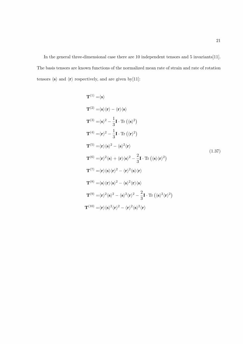
In the general three-dimensional case there are 10 independent tensors and 5 invariants[11].

The basis tensors are known functions of the normalized mean rate of strain and rate of rotation

tensors 〈s〉 and 〈r〉 respectively, and are given by[11]:

T(1) =〈s〉

T(2) =〈s〉〈r〉 − 〈r〉〈s〉

T(3) =〈s〉2 − 1

3I · Tr

(〈s〉2

)T(4) =〈r〉2 − 1

3I · Tr

(〈r〉2

)T(5) =〈r〉〈s〉2 − 〈s〉2〈r〉

T(6) =〈r〉2〈s〉+ 〈r〉〈s〉2 − 2

3I · Tr

(〈s〉〈r〉2

)T(7) =〈r〉〈s〉〈r〉2 − 〈r〉2〈s〉〈r〉

T(8) =〈s〉〈r〉〈s〉2 − 〈s〉2〈r〉〈s〉

T(9) =〈r〉2〈s〉2 − 〈s〉2〈r〉2 − 2

3I · Tr

(〈s〉2〈r〉2

)T(10) =〈r〉〈s〉2〈r〉2 − 〈r〉2〈s〉2〈r〉

(1.37)

22

where I is the three-dimensional identity tensor and Tr(A) corresponds to the operation of

taking the trace of tensor A. The five invariants are [11]:

λ1 =Tr(〈s〉2

)λ2 =Tr

(〈r〉2

)λ3 =Tr

(〈s〉3

)λ4 =Tr

(〈r〉2〈s〉

)λ5 =Tr

(〈r〉2〈s〉2

)

(1.38)

Note that the linear eddy viscosity model is recovered when g(1) = Cµ and g(n) = 0 for n > 1.

Finding the coefficients of Equation 1.36 is extremely diffcult for general three-dimensional

turbulent flows,with the aggravation that there is no obvious hierarchy of the basis components

[12].

There are additional defects of the representation of b via Equation 1.36 beyond its ob-

vious complexity. For example, the Reynolds stresses are not necessarily functions solely of

the mean rate of strain and rotation. Indeed, Reynolds stresses are non-local objects and rep-

resenting them as functions of local quantities is insufficient. Nevertheless, the representation

(Equation 1.36) for the eddy viscosity is appealing because the tensor basis is an integrity bases

which guarantees that b will satisfy Galilean invariance and remain a symmetric, anisotropic

tensor[11].

Although Equation 1.36 is very general, it is also extremely complicated to treat. Pope

itself, when proposing it, tuned the coefficients only for a particular two-dimensional flow case

23

and declared the three-dimensional form is so analytically intractable as to be of no value [11].

Indeed, for two dimensional flows there are only three linearly independent basis tensors T and

two non-zero independent invariants and therefore Equation 1.36 is much easier to treat.

When in a certain eddy viscosity model g(n) 6= 0 for n > 1, the model is said to be

nonlinear, since it entails the product of two or more second-order tensors. Nonlinear eddy

viscosity models, although more computationally expensive, have the potential to represent

additional flow physics, such as secondary flows and flows with mean streamline curvature [11].

Many nonlinear models have been developed, including quadratic eddy viscosity models, yet in

all of them only few -usually one more - of the g(n) coefficients are tuned due to the difficulty

of treating Equation 1.36 analytically.

1.4 Data Driven Turbulence Modeling

The term ’Data driven Turbulence Modelling’ usually refers to the attempt to deal with the

RANS models closure problem using machine learning techniques. In the following paragraphs,

the basics of neural networks basics be introduced and it will be explained how in this work

they were applied to turbulence modelling.

1.4.1 Neural Networks

Neural networks are a class of machine learning algorithms that have found applications in

a wide variety of fields, including computer vision, natural language processing and gaming.

Neural networks have shown to be particularly powerful in dealing with high dimensional have

shown to be particularly powerful in dealing with high-dimensional data and modeling nonlinear

and complex relationships [12].

24

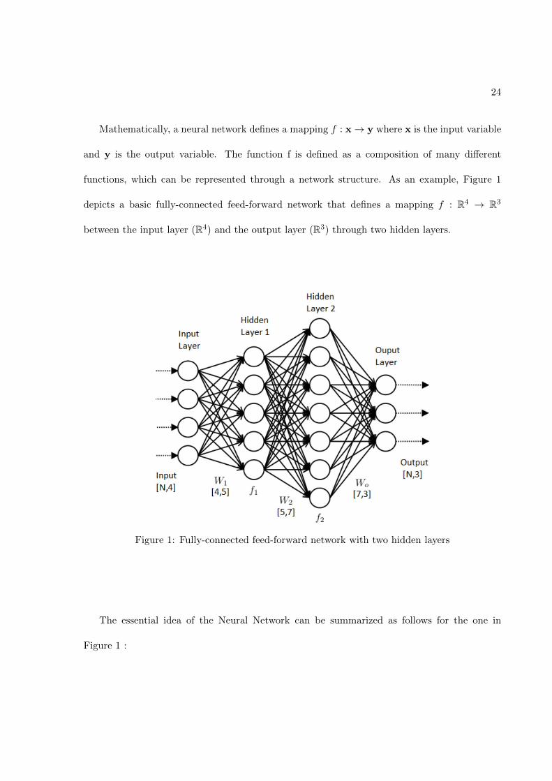
Mathematically, a neural network defines a mapping f : x→ y where x is the input variable

and y is the output variable. The function f is defined as a composition of many different

functions, which can be represented through a network structure. As an example, Figure 1

depicts a basic fully-connected feed-forward network that defines a mapping f : R4 → R3

between the input layer (R4) and the output layer (R3) through two hidden layers.

Figure 1: Fully-connected feed-forward network with two hidden layers

The essential idea of the Neural Network can be summarized as follows for the one in

Figure 1 :

25

1. The input layer here represents a 4-dimensional vector input x = [x1, x2, x3, x4]T with

each node in the layer standing for each component of the vector.

2. At the first hidden layer, the input x gets transformed into a 5-dimensional output.

This is done in two steps:

• First, an affine transformation is performed at each node j in the hidden layer:

z(1)j = b

(1)j +

3∑i=1

w(1)ij xi j = 1, 2, 3, 4, 5 (1.39)

where b(1)j is the bias value for node j and w

(1)ij is the weight value associated with

the arrow linking node i in the input layer to node j in the first hidden layer.

• Second, a nonlinear transformation is performed according to a pre-specified activa-

tion function, φ as:

f(1)j = φ

(z(1)j

)(1.40)

An example of an activation function is the ReLU function φ(z) = max (0, z)

Equation 1.40 and Equation 1.39 can be represented altogether in vector notation as:

f(1) = φ(W(1)x + b(1)

)(1.41)

26

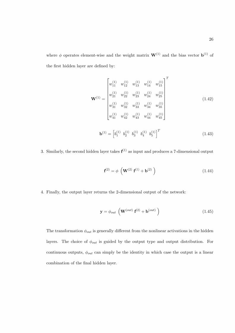
where φ operates element-wise and the weight matrix W(1) and the bias vector b(1) of

the first hidden layer are defined by:

W(1) =

w(1)11 w

(1)12 w

(1)13 w

(1)14 w

(1)15

w(1)21 w

(1)22 w

(1)23 w

(1)24 w

(1)25

w(1)31 w

(1)32 w

(1)33 w

(1)34 w

(1)35

w(1)41 w

(1)42 w

(1)43 w

(1)44 w

(1)45

T

(1.42)

b(1) =[b(1)1 b

(1)2 b

(1)3 b

(1)4 b

(1)5

]T(1.43)

3. Similarly, the second hidden layer takes f(1) as input and produces a 7-dimensional output

f(2) = φ(W(2) f(1) + b(2)

)(1.44)

4. Finally, the output layer returns the 2-dimensional output of the network:

y = φout

(W(out) f(2) + b(out)

)(1.45)

The transformation φout is generally different from the nonlinear activations in the hidden

layers. The choice of φout is guided by the output type and output distribution. For

continuous outputs, φout can simply be the identity in which case the output is a linear

combination of the final hidden layer.

27

The network just described is an example of a fully-connected, feed-forward network. It

is fully-connected because every node in a hidden layer is connected with all the nodes in the

previous and the following layers. It is feed-forward because the information flows in a forward

direction from input to output; there is no feedback connection where the output of any layer

is fed back into itself.

A fully-connected, feed-forward network is the most basic type of neural network and is

commonly referred to as a multilayer perceptron (MLP). Interestingly, it has been mathemati-

cally proven that MLPs are universal function approximators. The complexity of such a neural

network increases with the number of hidden layers (depth of the network) and the number of

nodes per hidden layer (width of the network).

Networks with more than one hidden layer are called deep neural networks.

1.4.2 Training of a Neural Network

The neural network expresses a functional form fNN which is completely defined by a set

of weights and biases denoted by W. This functional form is in general an approximation to

the true function f between the input and the output data.

To find the best function approximation, one has to solve an optimization problem that

minimizes the overall difference between f(x) and fNN (x) for all x in the input dataset to

obtain the model parameters. The process of finding the best model parameters (weights and

biases) is called model training or learning. Once the model is trained, its performance is

assessed on the validation dataset. Training and validation datasets are generated from the full

28

dataset by splitting it into validation and training portions. Often, the split is done with 20%

of the dataset used for validation and 80% used for training.

The overall difference between the true function and the approximation fNN is quantified

by a loss function. Typically, the choice of loss function is dependent on the particular problem.

A general form of the total loss function is:

L(W ) =1

N

N∑n=1

Ln(W ) (1.46)

where N is the total number of data points used for training and Ln is the loss function defined

for a single data point. A commonly used loss function is the mean squared error (MSE) loss:

L(W ) =1

N

N∑n=1

[(f(xn)− fNN (xn)

)·(f(xn)− fNN (xn)

)](1.47)

The stochastic gradient descent method(SGD) and its variants are used to iteratively find

parameters W that minimize the loss function of Equation 1.46. In standard Gradient Descent,

the model parameters W are updated according to:

W k = W k−1 − η∇L(W k) = W k−1 − η

(1

N

N∑n=1

∇Ln(W k)

)(1.48)

where W k are the model parameters at step k and η is the learning rate. This step repeats

until convergence is achieved to within a user-specified tolerance.

29

Although neural networks have impressive approximation properties, training them requires

the solution of a non-convex optimization problem. The classical gradient descent algorithm

(GD) has significant trouble in finding a global minimum and can often get stuck in a shallow

local minimum. The stochastic gradient descent algorithm provides a way of escaping from

local minima in an effort to get closer to a global minimum. In each iteration of the stochastic

gradient descent, the gradient ∇L(W ) is approximated by the gradient at a single data point

∇Ln(W ).

W k = W k−1 − η∇Ln(W k) (1.49)

The algorithm sweeps through the training data until convergence to a local minimum is

achieved. One full pass over the training data is called an epoch. Note that, generally, the

training data is randomly shuffled at the beginning of each epoch. This algorithm is stochastic

in the sense that the estimated gradient using a random data point is noisy whereas the gradient

calculated on the entire training data is exact. In practice, Mini-Batch Stochastic Gradient

Descent is employed, in which multiple data points are used in each iteration to approximate

the gradient.

The batch size M controls the number of random data points used per iteration. Hence at

each iteration the model parameters are updated as:

W k = W k−1 − η∇Lm(W k) = W k−1 − η

(1

M

M∑n=1

∇Ln(W k)

)(1.50)

30

The Mini-Batch Stochastic Gradient Descent is widely used since it combines the advantages of

Gradient Descent and Stochastic Gradient Descent methods : it proves indeed less noisy than

SGD and is more prone to overcome shallow local minimum compared to GD.

For parameter initialization, in most cases the initial weights are randomly sampled from a

uniform or normal distribution and the initial biases are set to 0.

Besides model parameters, the performance of a neural network changes with the external

configuration of the network model and the training process. The external configuration refers

to the number of hidden layers, the number of nodes per layer, the activation functions and the

learning rate. These are called the hyperparameters of a model.

The search for the best values of hyperparameters is called hyperparameter tuning. A

grid search can be performed to search combinations of values on a grid of parameters in the

hyperparameter space. A separate validation set that is different from the test set is used

for model evaluation during the tuning process. Alternatively, a Bayesian optimization of the

hyperparameters may also be performed [8].

1.4.3 The Tensor-Basis neural network

One possible way of applying machine learning techniques to turbulence modeling consists in

using them to determine a suitable function that satisfies Equation 1.35. In case neural networks

are chosen, the most straightforward idea would be to use the nine distinct components of 〈s〉

and 〈r〉 as inputs of the network for many points of the physical space in order to obtain the

corresponding b components in output.

31

Yet, in this case, it is not trivial for the neural network to learn some known physical prop-

erties of the nondimensional anisotropy tensor, such as the Galileian and rotational invariances.

Indeed, when the coordinate frame is rotated, the input components of the mean strain rate and

rotation rate tensors change and the anisotropy tensor in output is also rotated by the same an-

gle [5]. A ’physically correct’ neural network, given the same input tensors at different rotation

angles of the coordinates frames, should be able to predict in output the same anisotropy tensor

rotated by the same angles[5]. This result is not trivial to obtain with the intuitive network

architecture described above. One possible way of achieving that, would consist in training

the network on a set of observations including the same input and output tensors rotated at

different angles. In any case, however, the neural network would have to learn the invariance

properties of the output tensor on herself[5].

A special network architecture, which will be referred to as the tensor basis neural network

(TBNN), was proposed in 2016 by Julia Ling [8], in order to directly enforce invariance prop-

erties on the output anisotropy tensor. The key was to design a network architecture to match

the form of Equation 1.36. In this works’ neural network network, two input layers are present:

the invariants input layer and the tensor basis input layer. The invariants input layer is formed

by the five invariants λ1...λ5 and is followed by a series of hidden layers. The final hidden layer

has 10 nodes and represents the coefficients g(n) for n=1,..10 of Equation 1.36. The tensor

basis input layer is composed by the 10 invariant tensors T(n) for n=1,..10 of Equation 1.36.

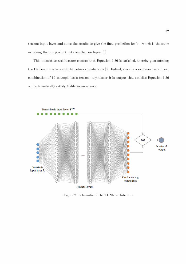
The merge output layer takes the element-wise products f the final hidden layer and the basis

32

tensors input layer and sums the results to give the final prediction for b - which is the same

as taking the dot product between the two layers [8].

This innovative architecture ensures that Equation 1.36 is satisfied, thereby guaranteeing

the Galileian invariance of the network predictions [8]. Indeed, since b is expressed as a linear

combination of 10 isotropic basis tensors, any tensor b in output that satisfies Equation 1.36

will automatically satisfy Galileian invariance.

Figure 2: Schematic of the TBNN architecture

33

In brief, the key idea is to employ the network to predict the coefficients g(n) from the

five invariants λ1...λ5 and to compute b accordingly as a linear combination of the tensor

invariants basis derived from 〈s〉 and 〈r〉, rather then directly deriving b from the two tensors’

components. When Ling, Jones and Templeton used neural networks to predict the Reynolds

stress anisotropy eigenvalues in 2016 , they reported a significant performance gain when a

rotationally invariant input feature set was used [5].

These results showed that embedding invariance properties into the machine learning model,

as the network architecture described in Figure 2 allows, is crucial for obtaining predictions with

higher accuracy.

1.4.4 Description of the proposed approach

The procedure followed by Ling [8]for employing the TBNN to improve Reynolds stresses

prediction in RANS simulations can be summarized as follows:

1. First of all, a neural network with the architecture described in Figure 2 is trained,

validated and tested on a database of nine different flows for which high fidelity (DNS

or well-resolved LES) as well as RANS results were available. The RANS data, obtained

using the k−ε model with the the LEVM (Equation 1.21) for the Reynolds stresses, were

used as the input to the Neural Network [8]. Therefore, each input observation consisted of

the quantities (invariants and tensors basis) derived from 〈s〉 and 〈r〉 at a particular point

in the space of the RANS solution. Each RANS simulations provides several observations

(the x in input to the network), theoretically one for each cell at which the numerical

solution of the flow field is available. The high-fidelity data were used to provide the truth

34

labels for the Reynolds stress anisotropy (the y that the network tries to replicate) during

model training and evaluation [8].

In brief, the network is trained to learn a function f : x(x, t)RANS → y(x, t)DNS -where x

is the set of neural network inputs - in this case the 5 invariants and the 10 basis tensors

at a particular point in the space - and y is the output of the network - namely the

nondimensional anisotropy stress tensor b at the corresponding point in space.

2. Once the neural network is trained, a desired RANS simualation is performed using a

standard model - such as the k − ε model withe the LEVM - as one would normally do.

The simulation can either be on a flow similar to one of the nine flows in the training

database -which should theoretically yield better results - or on a completely different

class of flow - in order to test the network model’s generality.

3. When the RANS simulation has converged, the invariants λi and the basis tensors T(n) are

computed at each point of the numerical solution using the tensors 〈s〉RANS and 〈r〉RANS

computed from the RANS solution flow fields 〈U〉RANS , kRANS , εRANS . Here the suffix

RANS refers to any quantity in output of the simulation run with the standard RANS

model chosen.

4. For each point in the space of the numerical solution, the the invariants λi and the basis

tensors T(n) are fed to the previously trained network. The output will be the predicted

anisotropy tensor bTBNN at the same point. The result will be an anisotropy stress tensor

field bTBNN (x, t).

35

5. Starting from the previous RANS solution, a new RANS simulation is run by imposing the

Reynolds stress anisotropy tensor field bTBNN (x, t) predicted by the TBNN as a constant

in the momentum equations and in the turbulent kinetic energy equation production term.

Since the Reynolds stresses are prescribed in the simulation, there will be no need for a

closure model like the LEVM.

6. The simulation is allowed to re-converge. At the end, the anisotropy stress tensor field

will be the same as the one predicted from the neural network, since bTBNN (x, t) is

held constant during the simulation. However the pressure and velocity fiels will be

different from the ones computed in the first simulation, since the LEVM model has been

replaced by an imposed known field of the anisotropy tensor. It is fair to assume that,

if bTBNN (x, t) proves a better approximation than bRANS(x, t) of the correct anisotropy

stress tensor field, then the new pressure and velocity fields will be closer to the correct

ones.

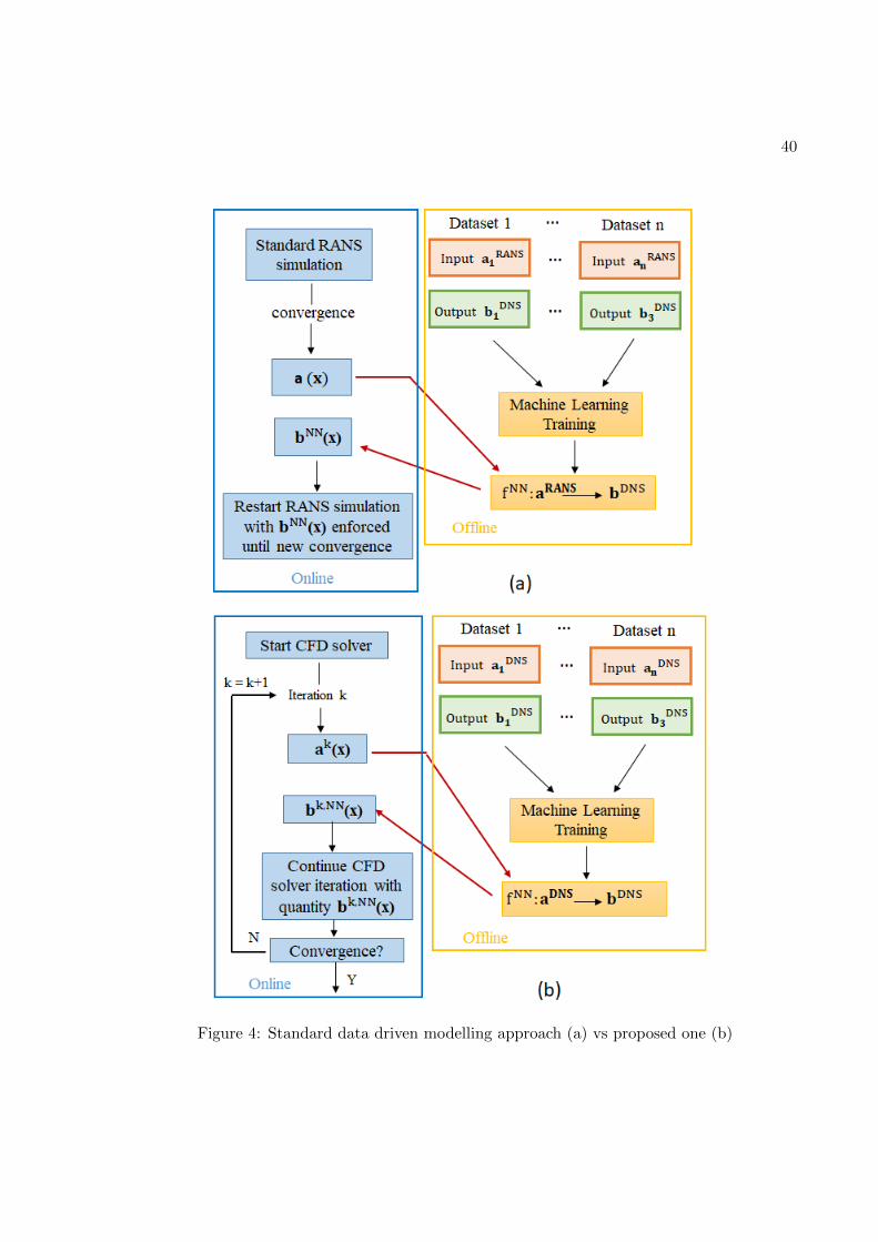
According to Ling’s procedure, the neural network is used as a ’post-processing’ tool to correct

the anisotropy stress tensor field predicted by the standard RANS simulation. Once the cor-

rected field is computed, it is injected in the RANS equations as a replacement of the LEVM

model and the simulation is allowed to re-converge.

The idea of using machine learning techniques as a post-processing correction tool of a

converged RANS solution has been applied in the majority of data driven turbulence modelling

approaches [8], [5], [1], [2], [4]. From a very general perspective, these approaches differ in the

machine learning method applied, in the quantity to predict - for example it can be the full

36

anisotropy stress tensor, its eigenvalues, a constant of the standard model to tune.. - or on the

inputs of the machine learning model. This entails that, since the neural network will be fed

with quantities computed from a RANS simulation, it has to be trained on a database of RANS

solutions. The ’post-processing’ approach, however, may present two key issues:

• Since the neural network is trained with quantities - the 5 invariants and the 10 basis

tensors in the case of Ling approach - derived from a RANS simulation performed with

a certain model X - such as k − ε, k − ω, S-A and so on - theoretically the same network

could not be applied to correct a simulation performed with a different model Y. Indeed,

due to the inaccuracies of these models, the result of a RANS solution will be generally

different when using different models, even though in most cases the difference is not huge.

However, if the network is trained to learn a function f : x(x, t)RANS,X → y(x, t)DNS -

where X is the RANS model used to compute the solution of the flows in the training

database - it is not clear why the same function should yield good performances when

correcting the fields computed with a different RANS model Y. This entails that , theo-

retically, a different neural network should be trained for each RANS model and for each

of its variants.

• In the case of Ling’s article, a neural network is trained to learn a function

f : Q(〈s〉RANS , 〈r〉RANS

)→ b(x, t)DNS where Q is the set of procedures to transfrom

〈s〉RANS and 〈r〉RANS into the correct inputs of the neural network. This attempts to

reproduce the function bij = bij(〈s〉, 〈r〉) whose validity is assumed in every eddy-viscosity

model. However, this realation holds for the ’true’ or ’correct’ fields, like the ones com-

37

puted with an high-fidelity DNS simulation.

In other words, relation (Equation 1.35) could be rewritten as : bDNSij = f(〈s〉DNS , 〈r〉)DNS

)and this relations, despite the limitations of its validity, has been taken as the starting

point for the developing of the most popular RANS closure models. However, there is no

physical hint that the nondimensional stress anisotropy tensor should depend on the veloc-

ity gradients computed via a RANS model which, in most cases, differ from the ’real’ DNS

ones. Hence a neural network trained to learn a function f : Q(〈s〉RANS , 〈r〉RANS

)→

b(x, t)DNS will not only have to learn how to relate b to velocity gradients but also how

to correct the RANS inputs.

In this work, a different approach is followed in the attempt to overcome the previous two

issues. It can be summarized as follows:

1. First of all, a tensor basis neural network with the same architecture of the one described

by Ling, will be validated and tested on a database of eight different flows for which hight

fidelity data(DNS or well-resolved LES) are available. The DNS 〈s〉 and 〈r〉 data -not the

RANS ones- will be used as the input to the Neural Network for each cell at which the

DNS solution of the flow field is available. The high-fidelity data will again be used to

provide the truth labels for the Reynolds stress anisotropy (the y that the network tries

to replicate) during model training and evaluation.

Hence, the network will be trained to learn a function f : x(x, t)DNS → y(x, t)DNS -

where x is the set of neural network inputs - in this case the 5 invariants and the 10 basis

38

tensors at a particular point in the space - and y is the output of the network - namely

the nondimensional anisotropy stress tensor b at the corresponding point in space.

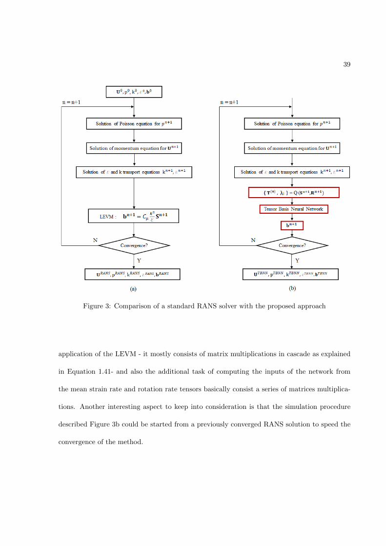
2. A RANS simulation with a chosen model - for example the k − ε one - will be run, but

the LEVM closure (Equation 1.21) will be replaced by the pre-trained neural network.

Hence, instead of using the network as a post-processing tool called at the end of a RANS

simulation to correct the obtained anisotropy stress tensor field, it will be called at each

iteration of the CFD solver to relate b to velocity gradients. Thererefore, theoretically,

at the end of the simulation the velocity gradients and the anisotropy stress tensor will

satisfy the network function learned from DNS data. A scheme of the idea is described

in Figure 3b for a general k − ε explicit RANS solver.

It is interesting to notice that this approach addresses both the issues pointed above. Firstly,

the neural network is trained to learn a relationship between the ’true’ velocity gradients and

the ’true’ anisotropy stress tensor f : Q(〈s〉DNS , 〈r〉DNS

)→ b(x, t)DNS as Equation 1.36 and

therefore it is trained to replicate exactly Equation 1.36. Secondly, since the network is trained

using DNS data, it could theoretically be used in all RANS models as a replacement to the

LEVM. As a consequence, there will be no need to train a different neural network for each

different RANS method and for each of its variants, thus improving considerably the generality

of the method.

Lastly, it is crucial to notice that the replacement of the LEVM with the neural network

would not entail a significant increase in the computational power when performing the simu-

lation. Indeed, the prediction time of the trained-network is negligible and comparable to the

39

Figure 3: Comparison of a standard RANS solver with the proposed approach

application of the LEVM - it mostly consists of matrix multiplications in cascade as explained

in Equation 1.41- and also the additional task of computing the inputs of the network from

the mean strain rate and rotation rate tensors basically consist a series of matrices multiplica-

tions. Another interesting aspect to keep into consideration is that the simulation procedure

described Figure 3b could be started from a previously converged RANS solution to speed the

convergence of the method.

40

Figure 4: Standard data driven modelling approach (a) vs proposed one (b)

CHAPTER 2

IMPLEMENTATION OF THE APPROACH

2.1 Development of a RANS CFD Solver

In order to test the data driven turbulence modelling method described in the previous

section, it is firstly necessary to develop a standard RANS solver. Once validated, it will be

possible to modify the solver to embed the pre-trained neural network as a replacement of the

LEVM. Hence, in the following sections, a detailed explanation of the steps employed to code

the solver will be given. The goal of the code it to solve the set of RANS partial differential

equations governing the evolution of turbulent flows, which will be later listed.

When writing a CFD solver, three main approaches are possible: finite difference method

(FDM), finite elements method (FEM) and finite volume method (FVM) [9]. They all consists

of different methods to solve a set of partial or ordinary differential equations on a discretized

geometry of the chosen problem. Here, the finite volume method is chosen. The choice is

motivated by the fact that the solver will be applied to cartesian, structured 2D geometries, for

which the FVM proves to be the easisest one to implement. With the term structured mesh or

structured grid, we refer to discretization of the physical space of the problem into geometrical

entities characterized by regular connectivity, so that the inner nodes have the same number

of elements around them and the mesh geometry can always be mapped into an ’equivalent’

41

42

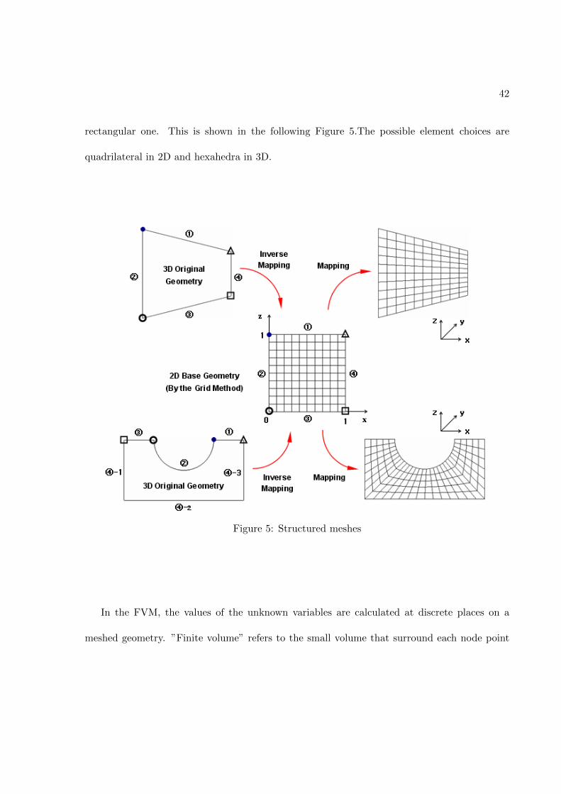
rectangular one. This is shown in the following Figure 5.The possible element choices are

quadrilateral in 2D and hexahedra in 3D.

Figure 5: Structured meshes

In the FVM, the values of the unknown variables are calculated at discrete places on a

meshed geometry. ”Finite volume” refers to the small volume that surround each node point

43

on a mesh. In the finite volume method, volume integrals in a partial differential equation

that contain a divergence term are transformed into surface integrals, using the Gauss theorem.

These terms are then treated as fluxes at the surfaces of each finite volume. Since the flux

entering a given volume is identical to that leaving the adjacent volume, these methods are

conservative. Another advantage of the finite volume method is that it is easily formulated to

allow for unstructured meshes. The method is commonly used in many computational fluid

dynamics packages [13].

As for the RANS turbulence model, a k−ε with LEVM model is chosen. Hence, along with

the average Navier-Stokes equations, two additional partial differential transport equations -

for ε and k - will have to be solved. One of the main issues with the k − ε family of models is

that, when used for wall-bounded turbulent flows- they are not valid all the way to the physical

walls. To work around this, three possible approaches can be followed [7]:

• Wall functions approach : One approach consists in modelling the boundary layer using

the renowned log-law correlation between the u component of the mean velocity field and

the viscous distance y+ from the wall- later defined - in the first cell adjacent to the

wall. In practice, the RANS equations are not solved within the buffer layer and viscous

sublayers - the regions of the flow closest to the wall - , yet rather a known relation

is directly enforced in the first cell of the mesh covering this whole near-wall region.

This approach is suitable for cases where wall-bounded effects are secondary, or the flow

undergoes geometry-induced separation [14]. The benefit is that wall functions allow the

use of a relatively coarse mesh in the near-wall region.

44

• Enhanced wall treatments This option combines a blended law-of-the wall and a two-layer

zonal model. This case involves the full numerical resolution of the boundary layer in the

viscous sublayer and in the buffer layer [15]. This approach is suitable for low-Reynolds

flows or for flows in which wall-bounded effects are of high priority (adverse pressure

gradients, aerodynamic drag, pressure drop, heat transfer, etc.) since it provides a more

accurate description of the near wall region. This method requires a fine-near wall mesh

capable of resolving the viscous sub-layer.

• low-Reynolds models: As in the Enhanced wall treatmen approach, the boundary layer

is numerically resolved up to the viscous sublayer. However, instead of using a two-layer

zonal model, low-Reynolds models make use of different blending functions applied to the

standard RANS equations. Those functions ensure that, far from the wall, the low-Re

model is equivalent to the standard RANS model while ,near the wall, the solution of the

blended equations leads to the correct wall relations [16]. This method as well requires a

fine-near wall mesh capable of resolving the viscous sub-layer.

An example of the typical grid resolutions required by the different approaches is shown in the

Figure 6.

Quantitatively, when a wall-functions approach is chosen, the first cell adjacent to the wall

must be placed at y+ > 30 - namely beyond the buffer layer - , whereas when a wall-resolved

method is used the first cell must be placed well within the viscous sublayer - usually at y+ ' 1.

Since the flows for which the RANS solver will be used are at relatively small Reynolds number,

a wall-functions approach would impose the definition of an excessively big first cell - since

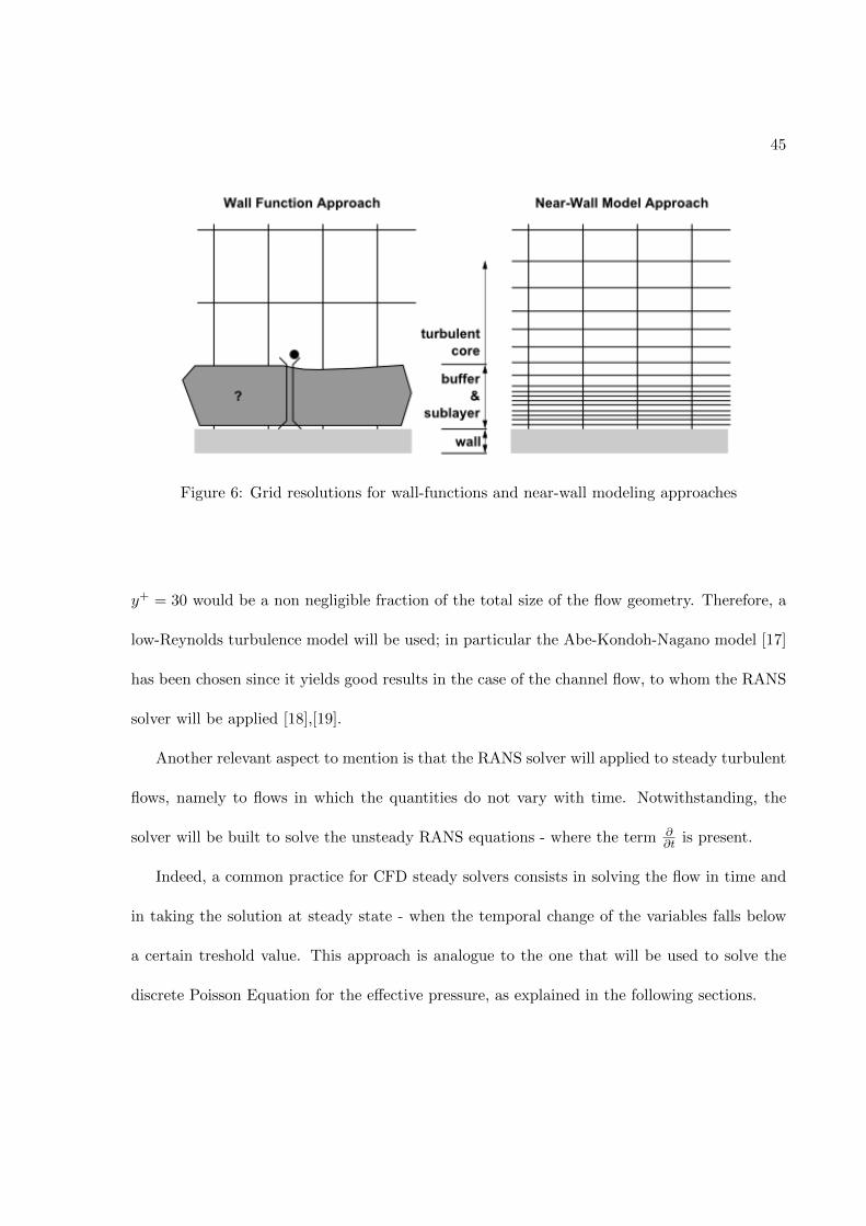
45

Figure 6: Grid resolutions for wall-functions and near-wall modeling approaches

y+ = 30 would be a non negligible fraction of the total size of the flow geometry. Therefore, a

low-Reynolds turbulence model will be used; in particular the Abe-Kondoh-Nagano model [17]

has been chosen since it yields good results in the case of the channel flow, to whom the RANS

solver will be applied [18],[19].

Another relevant aspect to mention is that the RANS solver will applied to steady turbulent

flows, namely to flows in which the quantities do not vary with time. Notwithstanding, the

solver will be built to solve the unsteady RANS equations - where the term ∂∂t is present.

Indeed, a common practice for CFD steady solvers consists in solving the flow in time and

in taking the solution at steady state - when the temporal change of the variables falls below

a certain treshold value. This approach is analogue to the one that will be used to solve the

discrete Poisson Equation for the effective pressure, as explained in the following sections.

46

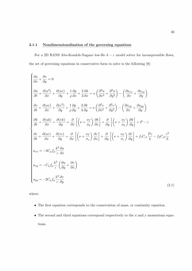
2.1.1 Nondimensionalization of the governing equations

For a 2D RANS Abe-Kondoh-Nagano low-Re k − ε model solver for incompressible flows,

the set of governing equations in conservative form to solve is the following [9]:

∂u

∂x+∂v

∂y= 0

∂u

∂t+∂(u2)

∂x+∂(uv)

∂y+

1

ρ

∂p

∂x+

2

3

∂k

∂x= ν

(∂2u

∂x2+∂2u

∂y2

)−(∂axx∂x

+∂axy∂y

)

∂v

∂t+∂(uv)

∂x+∂(v2)

∂y+

1

ρ

∂p

∂y+

2

3

∂k

∂y= ν

(∂2v

∂x2+∂2v

∂y2

)−(∂axy∂x

+∂ayy∂y

)

∂k

∂t+∂(uk)

∂x+∂(vk)

∂y=

∂

∂x

[(ν +

νTσk

)∂k

∂x

]+

∂

∂y

[(ν +

νTσk

)∂k

∂y

]+ P − ε

∂ε

∂t+∂(uε)

∂x+∂(vε)

∂y=

∂

∂x

[(ν +

νTσε

)∂ε

∂x

]+

∂

∂y

[(ν +

νTσε

)∂ε

∂y

]+ f1Cε1

Pε

k− f2Cε2

ε2

k

axx = −2Cµfµk2

ε

∂u

∂x

axy = −Cµfµk2

ε

(∂u

∂y+∂v

∂x

)

ayy = −2Cµfµk2

ε

∂v

∂y(2.1)

where:

• The first equation corresponds to the conservation of mass, or continuity equation.

• The second and third equations correspond respectively to the x and y momentum equa-

tions.

47

• The fourth equation corresponds to the transport equation for the turbulent kinetic energy

k.

• The fifth equation corresponds to the transport equation for the turbulent kinetic energy

dissipation rate ε.

• The last three equations correspond to the Linear Eddy Viscosity Model applied for each

non-zero component of the anisotropy stress tensor.

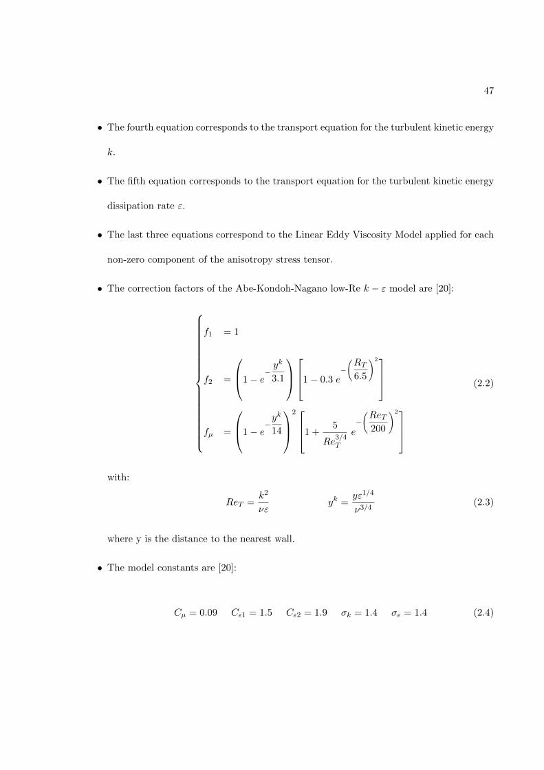
• The correction factors of the Abe-Kondoh-Nagano low-Re k − ε model are [20]:

f1 = 1

f2 =

1− e−yk

3.1

1− 0.3 e

−(RT6.5

)2

fµ =

1− e−yk

14

2 1 +

5

Re3/4T

e−(ReT200

)2

(2.2)

with:

ReT =k2

νεyk =

yε1/4

ν3/4(2.3)

where y is the distance to the nearest wall.

• The model constants are [20]:

Cµ = 0.09 Cε1 = 1.5 Cε2 = 1.9 σk = 1.4 σε = 1.4 (2.4)

48

• The terms u and v in (Equation 2.1) correspond the x and y component of the mean flow

field 〈U〉. The averaging operator 〈〉 has been omitted for the sake of brevity in all the

equations.

Now,the system in Equation 2.1 is expressed in dimensional form and therefore the solution

depends on the specific problem parameters - like the fluid viscosity or the geometry size . In

order to obtain a general form for the solution of the flow, it is necessary to nondimensionalize

the variables of the equations in Equation 2.1.

As a consequence, the following dimensionless parameters are introduced:

u∗ =u

Uv∗ =

v

Up∗ =

p

ρU2k∗ =

k

U2a∗ij =

aijU2

P ∗ =PL

U3

x∗ =x

Ly∗ =

y

Lt∗ = t

U

Lε∗ =

εL

U3ν∗T =

νTν

(2.5)

where L is a characteristic length and U is a characteristic velocity of the specific problem

considered. By substituting Equation 2.5 in the continuity equation of Equation 2.1 one obtains:

∂u∗

∂x∗U

L+∂v∗

∂y∗U

L= 0 (2.6)

from which it follows immediately:

∂u∗

∂x∗+∂v∗

∂y∗= 0 (2.7)

which corresponds to the nondimensional continuity equation.

49

Instead, by substituting Equation 2.5 in the momentum equation along x of Equation 2.1

one obtains:

U2

L

∂u∗

∂t∗+U2

L

∂(u∗2)

∂x∗+U2

L

∂(u∗v∗)

∂y∗+ρU2

L

1

ρ

∂p∗

∂x∗+

2

3

U2

L

∂k∗

∂x∗=

= ν

(U

L2

∂2u∗

∂x∗2+U

L2

∂2u∗

∂y∗2

)− U2

L

(∂a∗xx∂x

+∂a∗xy∂y

) (2.8)

Recalling that the Reynolds number is defined as:

Re =UL

ν(2.9)

if we divide Equation 2.8 by U2/L and substitute the expression Equation 2.9 we obtain:

∂u∗

∂t∗+∂(u∗2)

∂x∗+∂(u∗v∗)

∂y∗+∂p∗

∂x∗+

2

3

∂k∗

∂x∗=

1

Re

(∂2u∗

∂x∗2+∂2u∗

∂y∗2

)−(∂a∗xx∂x

+∂a∗xy∂y

)(2.10)

which corresponds to the non-dimensional momentum equation along x.

An analogous method is followed in order to nondimensionalize the momentum equation

along y. Indeed, by substituting Equation 2.5 in the y momentum equation of Equation 2.1 one

obtains:

U2

L

∂v∗

∂t∗+U2

L

∂(u∗v∗)

∂x∗+U2

L

∂(v∗2)

∂y∗+ρU2

L

1

ρ

∂p∗

∂y∗+

2

3

U2

L

∂k∗

∂y∗=

= ν

(U

L2

∂2v∗

∂x∗2+U

L2

∂2v∗

∂y∗2

)− U2

L

(∂a∗xy∂x

+∂a∗yy∂y

) (2.11)

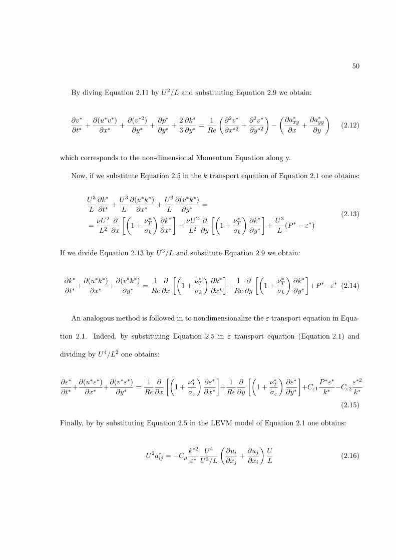
50

By diving Equation 2.11 by U2/L and substituting Equation 2.9 we obtain:

∂v∗

∂t∗+∂(u∗v∗)

∂x∗+∂(v∗2)

∂y∗+∂p∗

∂y∗+

2

3

∂k∗

∂y∗=

1

Re

(∂2v∗

∂x∗2+∂2v∗

∂y∗2

)−(∂a∗xy∂x

+∂a∗yy∂y

)(2.12)

which corresponds to the non-dimensional Momentum Equation along y.

Now, if we substitute Equation 2.5 in the k transport equation of Equation 2.1 one obtains:

U3

L

∂k∗

∂t∗+U3

L

∂(u∗k∗)

∂x∗+U3

L

∂(v∗k∗)

∂y∗=

=νU2

L2

∂

∂x

[(1 +

ν∗Tσk

)∂k∗

∂x∗

]+νU2

L2

∂

∂y

[(1 +

ν∗Tσk

)∂k∗

∂y∗

]+U3

L(P ∗ − ε∗)

(2.13)

If we divide Equation 2.13 by U3/L and substitute Equation 2.9 we obtain:

∂k∗

∂t∗+∂(u∗k∗)

∂x∗+∂(v∗k∗)

∂y∗=

1

Re

∂

∂x

[(1 +

ν∗Tσk

)∂k∗

∂x∗

]+

1

Re

∂

∂y

[(1 +

ν∗Tσk

)∂k∗

∂y∗

]+P ∗−ε∗ (2.14)

An analogous method is followed in to nondimensionalize the ε transport equation in Equa-

tion 2.1. Indeed, by substituting Equation 2.5 in ε transport equation (Equation 2.1) and

dividing by U4/L2 one obtains:

∂ε∗

∂t∗+∂(u∗ε∗)

∂x∗+∂(v∗ε∗)

∂y∗=

1

Re

∂

∂x

[(1 +

ν∗Tσε

)∂ε∗

∂x∗

]+

1

Re

∂

∂y

[(1 +

ν∗Tσε

)∂ε∗

∂y∗

]+Cε1

P ∗ε∗

k∗−Cε2

ε∗2

k∗

(2.15)

Finally, by by substituting Equation 2.5 in the LEVM model of Equation 2.1 one obtains:

U2a∗ij = −Cµk∗2

ε∗U4

U3/L

(∂ui∂xj

+∂uj∂xi

)U

L(2.16)

51

and by dividing Equation 2.16 by U2 we get to:

a∗ij = −Cµk∗2

ε∗

(∂ui∂xj

+∂uj∂xi

)(2.17)

The last step consists in expressing ReT and yk of the Abe-Kondoh-Nagano model as a

function of the nondimensional variables:

ReT =1

ν

k2∗

ε∗U4

U3/L= Re

k2∗

ε∗

yk∗ =yk

L=(y∗ε∗1/4

)L

(U3

L

)1/4

ν3/4 =(y∗ε∗1/4

)Re3/4

(2.18)

52

Hence, the conservative nondimensional form of the governing equations of the 2D RANS

Abe-Kondoh-Nagano low-Re k − ε model are:

∂u∗

∂x∗+∂v∗

∂y∗= 0

∂u∗

∂t∗+∂(u∗2)

∂x∗+∂(u∗v∗)

∂y∗+∂p∗

∂x∗+

2

3

∂k∗

∂x∗=

1

Re

(∂2u∗

∂x∗2+∂2u∗

∂y∗2

)−(∂a∗xx∂x

+∂a∗xy∂y

)

∂v∗

∂t∗+∂(u∗v∗)

∂x∗+∂(v∗2)

∂y∗+∂p∗

∂y∗+

2

3

∂k∗

∂y∗=

1

Re

(∂2v∗

∂x∗2+∂2v∗

∂y∗2

)−(∂a∗xy∂x

+∂a∗yy∂y

)

∂k∗

∂t∗+∂(u∗k∗)

∂x∗+∂(v∗k∗)

∂y∗=

1

Re

∂

∂x

[(1 +

ν∗Tσk

)∂k∗

∂x∗

]+

1

Re

∂

∂y

[(1 +

ν∗Tσk

)∂k∗

∂y∗

]+ P ∗ − ε∗

∂ε∗

∂t∗+∂(u∗ε∗)

∂x∗+∂(v∗ε∗)

∂y∗=

1

Re

∂

∂x

[(1 +

ν∗Tσε

)∂ε∗

∂x∗

]+

1

Re

∂

∂y

[(1 +

ν∗Tσε

)∂ε∗

∂y∗

]+ Cε1

P ∗ε∗

k∗− Cε2

ε∗2

k∗

a∗xx = −2Cµfµk∗2

ε∗∂u∗

∂x∗

a∗xy = −Cµfµk∗2

ε∗

(∂u∗

∂y∗+∂v∗

∂x∗

)

a∗yy = −2Cµfµk∗2

ε∗∂v∗

∂y∗

(2.19)

2.1.2 The Marker and Cell (MAC) method

In order to solve numerically the equations governing the Initial and Boundary value problem

described above, the unsteady explicit MAC (Marker in Cell) method is used. The method was

firstly introduced by Harlow and Welch in in order to numerically solve the time-dependent

flow of an incompressible liquid whose boundary is partly confined and partly free [21].

53

A staggered arrangement is chosen for the computation of the variables on the grid [9]. In

this grid’s arrangement the pressure,the velocity components and the turbulence quantities are

not stored on the same grid points: in this case, the pressure is computed at the center of the

cells, v is computed in correspondence of the upper edge of the cell, u in correspondence of the

right edge and the turbulence quantities, -such as k, ε- are stored at the cell vertex [22].

The production terms in k and ε transport equations are evaluated at the same locations

of k, ε, namely the cell vertices, where the strain and rotation rate tensors are computed and

the eddy viscosity calculated from k and ε at these cell vertices are directly used to calculate

the turbulent stress tensor. In this way, the Navier-Stokes equations and the k and ε transport

equations are coupled as closely as possible, as mentioned in [22].

Whenever the value of a variable is required in a grid location different from the one where

the variable is computed and stored, simple interpolation is used as it will be later shown. The

main advantage of such an arrangement is that it helps avoiding some types of convergence and

oscillation problems in the velocity and pressure fields [23] and guarantees a strong coupling

between the Navier-Stokes equations and the k and ε transport equations [22].

In the following, when referring to quantities computed at the edges of the Control Volumes,

fractional indices are used. However, when writing the code, the velocity and turbulent quan-

tities’ values will be stored with indices corresponding to the position of the center of the cell.

Since when plotting the solution both the pressure and velocity field must be referred to the

same grid locations, the value of u and v at the center of each cell is computed by interpolation

54

between consecutive edges. The following Figure 7 shows how the staggered arrangement is

implemented.

Figure 7: Staggered Arrangement

In the following, we will refer only to nondimensional quantities for pressure and velocity.

In order to ease the writing, the superscript * will be omitted. We will aslo refer to the column

index as i and to the row index as j. The center of each cell corresponds to an indices pair

(i,j), so that we will refer to the pressure at the center of the (j,i) cell as pji. For the velocity

components and the turbulent quantities, the fractional index notation will be used, as shown

in Figure 7a.

55

The MAC method is explicit [24] this means that the velocity field at time tn+1 is a function

of variables already computed at time tn. The method makes use of finite volumes approxima-

tions applied to the full Navier-Stokes equations and the numerical scheme is Forward-in-Time

Central-in-Space [21].

2.1.3 Discretization of the equations

In this section, the Navier-stokes momentum equations and the k and ε transport equations

are discretized according to the Finite Volume Method. The discretization procedure will be

carried out on cartesian, non uniform grid. This means that the grid is composed of adjacent

rectangles which may have differnt dimesions ∆x and ∆y. For the continuity equation, a special

treatment is required. This will be examined in the following section.

Before starting with the discretization, it is useful to remind the expression for the centered

discretizaion of the first derivative on a non-uniform grid [9]:

(∂φ

∂x

)i

' φi+1∆xi

(∆xi + ∆xi+1)(∆xi)+ φi

∆xi+1 −∆xi∆xi+1∆xi

− φi−1∆xi+1

(∆xi + ∆xi+1)(∆xi+1)(2.20)

where ∆xi = xi−xi−1 , ∆xi+1 = xi+1−xi and φi corresponds to the numerical approximation

of variable φ at position xi of the discretization grid, as shown in Figure 8.

In case of uniform grid ∆xi = ∆xi+1 = ∆x, equation (Equation 2.21) is reduced to :

(∂φ

∂x

)i

' φi+1 − φi−12∆x

(2.21)

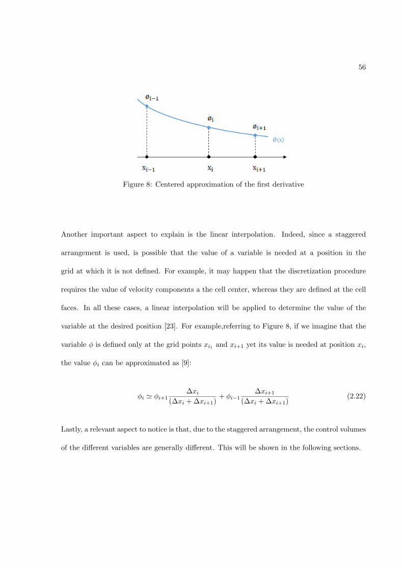
56

Figure 8: Centered approximation of the first derivative

Another important aspect to explain is the linear interpolation. Indeed, since a staggered

arrangement is used, is possible that the value of a variable is needed at a position in the

grid at which it is not defined. For example, it may happen that the discretization procedure

requires the value of velocity components a the cell center, whereas they are defined at the cell

faces. In all these cases, a linear interpolation will be applied to determine the value of the

variable at the desired position [23]. For example,referring to Figure 8, if we imagine that the

variable φ is defined only at the grid points xi1 and xi+1 yet its value is needed at position xi,

the value φi can be approximated as [9]:

φi ' φi+1∆xi

(∆xi + ∆xi+1)+ φi−1

∆xi+1

(∆xi + ∆xi+1)(2.22)

Lastly, a relevant aspect to notice is that, due to the staggered arrangement, the control volumes

of the different variables are generally different. This will be shown in the following sections.

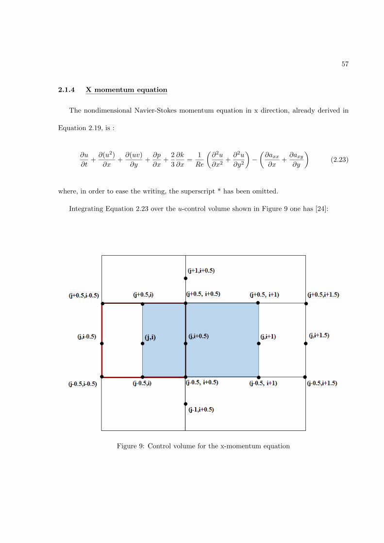
57

2.1.4 X momentum equation

The nondimensional Navier-Stokes momentum equation in x direction, already derived in

Equation 2.19, is :

∂u

∂t+∂(u2)

∂x+∂(uv)

∂y+∂p

∂x+

2

3

∂k

∂x=

1

Re

(∂2u

∂x2+∂2u

∂y2

)−(∂axx∂x

+∂axy∂y

)(2.23)

where, in order to ease the writing, the superscript * has been omitted.

Integrating Equation 2.23 over the u-control volume shown in Figure 9 one has [24]:

Figure 9: Control volume for the x-momentum equation

58

∫∫∂u

∂tdxdy +

∫∫∂

∂x

(u2 + axx −

1

Re

∂u

∂x

)dxdy +

∫∫∂

∂y

(uv + axy −

1

Re

∂u

∂y

)dxdy∫∫

∂peff∂x

dxdy = 0

(2.24)

where we have substituted peff = p+ 2k/3.

Application of the Green theorem to the above expression and use of MAC method for the

time discretization leads to:

∆x∆y

∆t(un+1j,i+ 1

2

− un) +(Exj,i+1 − Exj,i

)∆y +

(F xj+ 1

2,i+ 1

2

− F xj− 1

2,i+ 1

2

)∆x

+(pn+1eff,j,i+1 − p

n+1eff,j,i

)∆y = 0

(2.25)

or equivalently :

(un+1j,i+ 1

2

− unj,i+ 1

2

)

∆t+

(Exj,i+1 − Exj,i

)∆x

+

(F xj+ 1

2,i+ 1

2

− F xj− 1

2,i+ 1

2

)∆y

+

(pn+1eff,j,i+1 − p

n+1eff,j,i

)∆x

= 0

(2.26)

where ∆x = xj,i+1 − xj,i and ∆y = yj+ 12,i+ 1

2− yj− 1

2,i+ 1

2are the dimensions of the (j,i) x-

momentum Control Volume , ∆t = tn+1 − tn, Ex and F x are the axial and trasversal fluxes of

x-momentum defined as:

Ex = u2 + axx −1

Re

∂u

∂xF x = uv + axy −

1

Re

∂u

∂y(2.27)

59

whose discretized forms for Equation 2.25 can be obtained using linear interpolation (Equation 2.22)

and the expression for the first derivative in Equation 2.21:

Exj,i+1 =

(unj,i+ 3

2

+ unj,i+ 1

2

2

)2

+

(anxx,j+ 1

2,i+ 1

2

+ anxx,j− 1

2,i+ 1

2

+ anxx,j+ 1

2,i+ 3

2

+ anxx,j− 1

2,i+ 3

2

4

)

− 1

Re

(unj,i+ 3

2

− unj,i+ 1

2

xj,i+ 32− xj,i+ 1

2

)

Exj,i =

(unj,i+ 1

2

+ unj,i− 1

2

2

)2

+

(anxx,j+ 1

2,i+ 1

2

+ anxx,j− 1

2,i+ 1

2

+ anxx,j+ 1

2,i− 1

2

+ anxx,j− 1

2,i− 1

2

4

).

− 1

Re

(unj,i+ 1

2

− unj,i− 1

2

xj,i+ 12− xj,i− 1

2

)

F xj+ 1

2,i+ 1

2

=

unj+1,i+ 12

(yj+ 1

2,i+ 1

2− yj,i+ 1

2

)+ un

j,i+ 12

(yj+1,i+ 1

2− yj+ 1

2,i+ 1

2

)yj+1,i+ 1

2− yj,i+ 1

2

··

vnj+ 12,i+1

(xj+ 1

2,i+ 1

2− xj+ 1

2,i

)+ vn

j+ 12,i

(xj+ 1

2,i+1 − xj+ 1

2,i+ 1

2

)xj+ 1

2,i+1 − xj+ 1

2,i

− 1

Re

(unj+1,i+ 1

2

− unj,i+ 1

2

yj+1,i+ 12− yj,i+ 1

2

)+ an

xy,j+ 12,i+ 1

2

F xj− 1

2,i+ 1

2

=

unj,i+ 12

(yj− 1

2,i+ 1

2− yj−1,i+ 1

2

)+ un

j−1,i+ 12

(yj,i+ 1

2− yj− 1

2,i+ 1

2

)yj,i+ 1

2− yj−1,i+ 1

2

··

vnj− 12,i+1

(xj− 1

2,i+ 1

2− xj− 1

2,i

)+ vn

j− 12,i

(xj− 1

2,i+1 − xj− 1

2,i+ 1

2

)xj− 1

2,i+1 − xj− 1

2,i

− 1

Re

(unj,i+ 1

2

− unj−1,i+ 1

2

yj,i+ 12− yj−1,i+ 1

2

)+ an

xy,j− 12,i+ 1

2

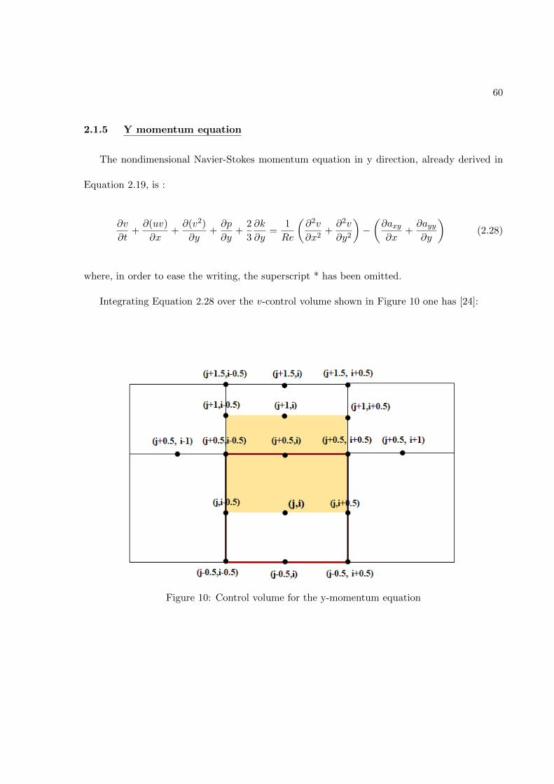
60

2.1.5 Y momentum equation

The nondimensional Navier-Stokes momentum equation in y direction, already derived in

Equation 2.19, is :

∂v

∂t+∂(uv)

∂x+∂(v2)

∂y+∂p

∂y+

2

3

∂k

∂y=

1

Re

(∂2v

∂x2+∂2v

∂y2

)−(∂axy∂x

+∂ayy∂y

)(2.28)

where, in order to ease the writing, the superscript * has been omitted.

Integrating Equation 2.28 over the v-control volume shown in Figure 10 one has [24]:

Figure 10: Control volume for the y-momentum equation

61

∫∫∂v

∂tdxdy +

∫∫∂

∂x

(uv + axy −

1

Re

∂v

∂x

)dxdy +

∫∫∂

∂y

(v2 + ayy −

1

Re

∂v

∂y

)dxdy

+

∫∫∂peff∂y

dxdy = 0

(2.29)

where we have substituted peff = p+ 2k/3.

Application of the Green theorem to the above expression and use of MAC method for the

time discretization leads to:

∆x∆y

∆t(vn+1j+ 1

2,i− vn

j+ 12,i) +

(Eyj,i+1 − E

yj,i

)∆y +

(F yj+ 1

2,i+ 1

2

− F yj− 1

2,i+ 1

2

)∆x

+(pn+1eff,j+1,i − p

n+1eff,j,i

)∆x = 0

(2.30)

or equivalenlty :

(vn+1j+ 1

2,i− vn

j+ 12,i)

∆t+

(Exj,i+1 − Exj,i

)∆x

+

(F xj+ 1

2,i+ 1

2

− F xj− 1

2,i+ 1

2

)∆y

+

(pn+1eff,j+1,i − p

n+1eff,j,i

)∆y

= 0

(2.31)

where ∆x = xj+ 12,i+ 1

2− xj+ 1

2,i− 1

2and ∆y = yj+1,i − yj,i are the x and y dimension of the (j,i)

y-momentum Control Volume ,∆t = tn+1 − tn, Ey and F y are the axial and trasversal fluxes

of y-momentum defined as:

Ey = uv + axy −1

Re

∂v

∂xF y = v2 + ayy −

1

Re

∂v

∂y(2.32)

62

whose discretized forms for Equation 2.30 can be obtained using (Equation 2.22) and the ex-

pression for the first derivative in Equation 2.21:

F yj+1,i =

(vnj+ 3

2,i

+ vnj+ 1

2,i

2

)2

+

(anyy,j+ 1

2,i+ 1

2

+ anyy,j+ 1

2,i− 1

2

+ anyy,j+ 3

2,i+ 1

2

+ anyy,j+ 3

2,i− 1

2

4

)

− 1

Re

(vnj+ 3

2,i− vn

j+ 12,i

yj+ 32,i − yj+ 1

2, i

)

F yj,i =

(vnj+ 1

2,i

+ vnj− 1

2,i

2

)2

+

(anyy,j− 1

2,i+ 1

2

+ anyy,j− 1

2,i− 1

2

+ anyy,j+ 1

2,i+ 1

2

+ anyy,j+ 1

2,i− 1

2

4

)

− 1

Re

(vnj+ 1

2,i− vn

j− 12,i

yj+ 12,i − yj− 1

2, i

)

Eyj+ 1

2,i+ 1

2

=

unj+1,i+ 12

(yj+ 1

2,i+ 1

2− yj,i+ 1

2

)+ un

j,i+ 12

(yj+1,i+ 1

2− yj+ 1

2,i+ 1

2

)yj+1,i+ 1

2− yj,i+ 1

2

··

vnj+ 12,i+1

(xj+ 1

2,i+ 1

2− xj+ 1

2,i

)+ vn

j+ 12,i

(xj+ 1

2,i+1 − xj+ 1

2,i+ 1

2

)xj+ 1

2,i+1 − xj+ 1

2,i

− 1

Re

(vnj+ 1

2,i+1− vn

j+ 12,i

xj+ 12,i+1 − xj+ 1

2,i

)+ an

xy,j+ 12,i+ 1

2

Eyj+ 1

2,i− 1

2

=

unj+1,i− 12

(yj+ 1

2,i− 1

2− yj,i− 1

2

)+ un

j,i− 12

(yj+1,i− 1

2− yj+ 1

2,i− 1

2

)yj+1,i− 1

2− yj,i− 1

2

··

vnj+ 12,i

(xj+ 1

2,i− 1

2− xj+ 1

2,i−1

)+ vn

j+ 12,i−1

(xj+ 1

2,i − xj+ 1

2,i− 1

2

)xj+ 1

2,i − xj+ 1

2,i−1

− 1

Re

(vnj+ 1

2,i− vn

j+ 12,i−1

xj+ 12,i − xj+ 1

2,i−1

)+ an

xy,j+ 12,i− 1

2

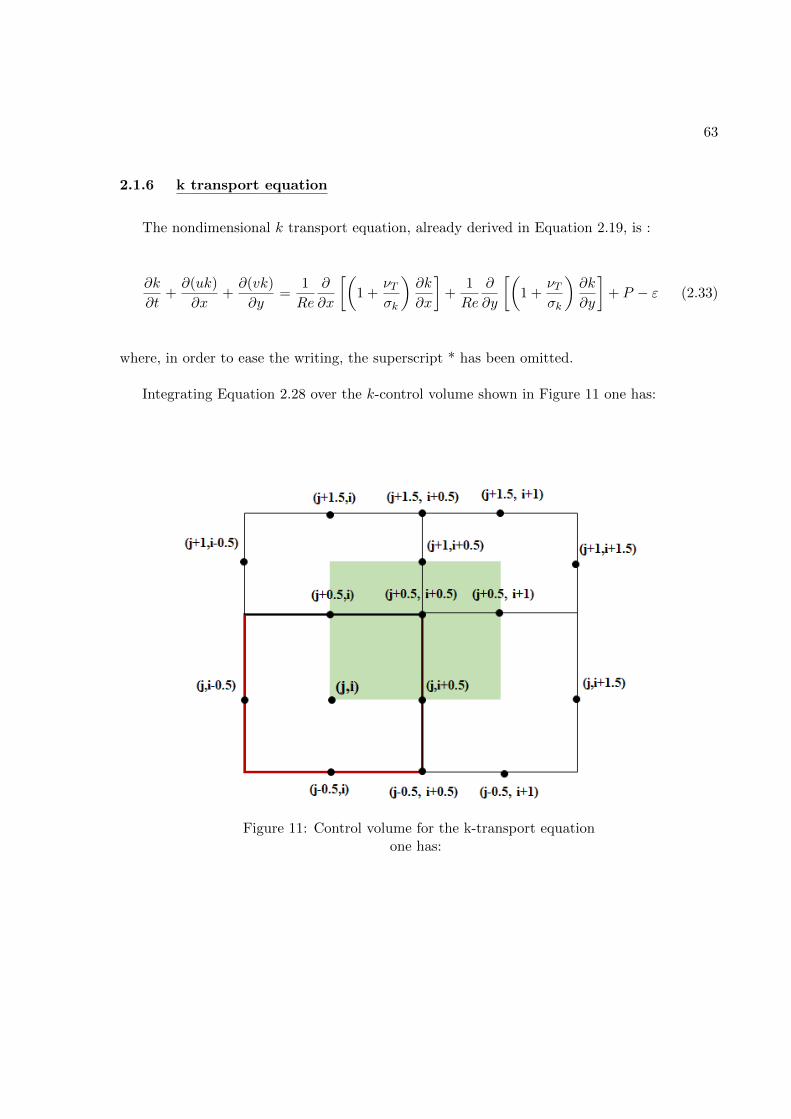
63

2.1.6 k transport equation

The nondimensional k transport equation, already derived in Equation 2.19, is :

∂k

∂t+∂(uk)

∂x+∂(vk)

∂y=

1

Re

∂

∂x

[(1 +

νTσk

)∂k

∂x

]+

1

Re

∂

∂y

[(1 +

νTσk

)∂k

∂y

]+ P − ε (2.33)

where, in order to ease the writing, the superscript * has been omitted.

Integrating Equation 2.28 over the k-control volume shown in Figure 11 one has:

Figure 11: Control volume for the k-transport equationone has:

64

∫∫∂k

∂tdxdy +

∫∫∂

∂x

[uk −

(1 +

νTσk

)∂k

∂x

]dxdy +

∫∫∂

∂y

[vk −

(1 +

νTσk

)∂k

∂y

]dxdy

+

∫∫(P − ε) dxdy = 0

(2.34)

Application of the Green theorem to the above expression and use of MAC method for the

time discretization leads to:

∆x∆y

∆t(kn+1j+ 1

2,i+ 1

2

− knj+ 1

2,i+ 1

2

) +(Ekj+ 1

2,i+1− Ek

j+ 12,i

)∆y +

(F kj+1,i+ 1

2

− F kj,i+ 1

2

)∆x

+ (Pnj+ 1

2,i+ 1

2

− εnj+ 1

2,i+ 1

2

)∆x∆y = 0

(2.35)

or equivalenty :

(kn+1j+ 1

2,i+ 1

2

− knj+ 1

2,i+ 1

2

)

∆t+

(Ekj+ 1

2,i+1− Ek

j+ 12,i

)∆x

+

(F kj+1,i+ 1

2

− F kj,i+ 1

2

)∆y

+Pnj+ 1

2,i+ 1

2

−εnj+ 1

2,i+ 1

2

= 0

(2.36)

where ∆x = xj+ 12,i+1 − xj+ 1

2,i and ∆y = yj+ 1

2,i+ 1

2− yj− 1

2,i+ 1

2are the x and y dimension of

the (j,i) k-transport Control Volume ,∆t = tn+1 − tn, Ek and F k are the axial and transversal

fluxes of k defined as:

Ek = uk −(

1 +νTσk

)∂k

∂xF k = vk −

(1 +

νTσk

)∂k

∂y(2.37)

65

whose discretized forms for Equation 2.35 can be obtained using linear interpolation in Equa-

tion 2.22 and the expression for the first derivative of Equation 2.21:

Ekj+ 1

2,i+1

=

[(unj,i+ 1

2

+ unj,i+ 3

2

2

)(yj+1,i+1 − yj+ 12,i+1

yj+1,i+1 − yj,i+1

)

+

(unj+1,i+ 1

2

+ unj+1,i+ 3

2

2

)(yj+ 12,i+1 − yj,i+1

yj+1,i+1 − yj,i+1

)]·

(knj+ 1

2,i+ 3

2

+ knj+ 1

2,i+ 1

2

2

)

−

(1 +

νnT,j+ 1

2,i+ 3

2

+ νnT,j+ 1

2,i+ 1

2

2σk

)(knj+ 1

2,i+ 3

2

− knj+ 1

2,i+ 1

2

xj+ 12,i+ 3

2− xj+ 1

2,i+ 1

2

)

Ekj+ 1

2,i

=

[(unj,i− 1

2

+ unj,i+ 1

2

2

)(yj+1,i − yj+ 12,i

yj+1,i − yj,i

)+

(unj+1,i− 1

2

+ unj+1,i+ 1

2

2

)(yj+ 12,i − yj,i

yj+1,i − yj,i

)]·

·

(knj+ 1

2,i+ 1

2

+ knj+ 1

2,i− 1

2

2

)−

(1 +

νnT,j+ 1

2,i+ 1

2

+ νnT,j+ 1

2,i− 1

2

2σk

)(knj+ 1

2,i+ 1

2

− knj+ 1

2,i− 1

2

xj+ 12,i+ 1

2− xj+ 1

2,i− 1

2

)

F kj+1,i+ 1

2

=

[(vnj+ 3

2,i+1

+ vnj+ 1

2,i+1

2

)(xj+1,i+ 12− xj+1,i

xj+1,i+1 − xj+1,i

)

+

(vnj+ 3

2,i

+ vnj+ 1

2,i

2

)(xj+1,i+1 − xj+1,i+ 12

xj+1,i+1 − xj+1,i

)]·

(knj+ 3

2,i+ 1

2

+ knj+ 1

2,i+ 1

2

2

)

−

(1 +

νnT,j+ 3

2,i+ 1

2

+ νnT,j+ 1

2,i+ 1

2

2σk

)(knj+ 3

2,i+ 1

2

− knj+ 1

2,i+ 1

2

yj+ 32,i+ 1

2− yj+ 1

2,i+ 1

2

)

F kj,i+ 1

2

=

[(vnj+ 1

2,i+1

+ vnj− 1

2,i+1

2

)(xj,i+ 12− xj,i

xj,i+1 − xj,i

)+

(vnj+ 1

2,i

+ vnj− 1

2,i

2

)(xj,i+1 − xj,i+ 12

xj,i+1 − xj,i

)]·

·

(knj+ 1

2,i+ 1

2

+ knj− 1

2,i+ 1

2

2

)−

(1 +

νnT,j+ 1

2,i+ 1

2

+ νnT,j− 1

2,i+ 1

2

2σk

)(knj+ 1

2,i+ 1

2

− knj− 1

2,i+ 1

2

yj+ 12,i+ 1

2− yj− 1

2,i+ 1

2

)

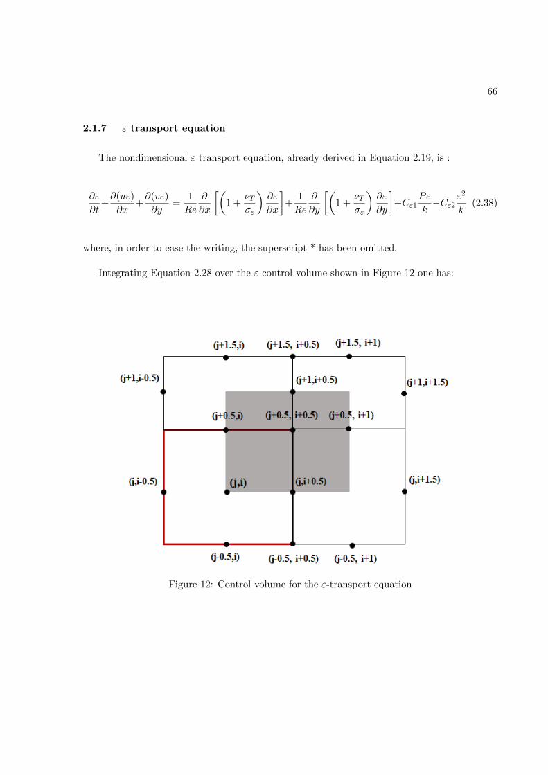
66

2.1.7 ε transport equation

The nondimensional ε transport equation, already derived in Equation 2.19, is :

∂ε

∂t+∂(uε)

∂x+∂(vε)

∂y=

1

Re

∂

∂x

[(1 +

νTσε

)∂ε

∂x

]+

1

Re

∂

∂y

[(1 +

νTσε

)∂ε

∂y

]+Cε1

Pε

k−Cε2

ε2

k(2.38)

where, in order to ease the writing, the superscript * has been omitted.

Integrating Equation 2.28 over the ε-control volume shown in Figure 12 one has:

Figure 12: Control volume for the ε-transport equation

67

∫∫∂ε

∂tdxdy +

∫∫∂

∂x

[uε−

(1 +

νTσε

)∂ε

∂x

]dxdy +

∫∫∂

∂y

[vε−

(1 +

νTσε

)∂ε

∂y

]dxdy

+

∫∫ε

k(Cε1P − Cε2ε) dxdy = 0

(2.39)

Application of the Green theorem to the above expression and use of MAC method for the

time discretization leads to:

∆x∆y

∆t(εn+1j+ 1

2,i+ 1

2

− εnj+ 1

2,i+ 1

2

) +(Eεj+ 1

2,i+1− Eε

j+ 12,i

)∆y +

(F εj+1,i+ 1

2

− F εj,i+ 1

2

)∆x

+εnj+ 1

2,i+ 1

2

knj+ 1

2,i+ 1

2

(Cε1Pnj+ 1

2,i+ 1

2

− Cε2εnj+ 12,i+ 1

2

)∆x∆y = 0

(2.40)

or equivalenty :

(εn+1j+ 1

2,i+ 1

2

− εnj+ 1

2,i+ 1

2

)

∆t+

(Eεj+ 1

2,i+1− Eε

j+ 12,i

)∆x

+

(F εj+1,i+ 1

2

− F εj,i+ 1

2

)∆y

+

εnj+ 1

2,i+ 1

2

knj+ 1

2,i+ 1

2

(Cε1Pnj+ 1

2,i+ 1

2

− Cε2εnj+ 12,i+ 1

2

) = 0

(2.41)

where ∆x = xj+ 12,i+1 − xj+ 1

2,i and ∆y = yj+ 1

2,i+ 1

2− yj− 1

2,i+ 1

2are the x and y dimension of the

(j,i) ε transport Control Volume ,∆t = tn+1− tn, Eε and F ε are the axial and trasversal fluxes

of ε defined as:

Eε = uε−(

1 +νTσε

)∂ε

∂xF ε = vε−

(1 +

νTσε

)∂ε

∂y(2.42)

68

whose discretized forms for Equation 2.40 can be obtained using linear interpolations of Equa-

tion 2.22 and the expression for the first derivative in Equation 2.21:

Eεj+ 1

2,i+1

=

[(unj,i+ 1

2

+ unj,i+ 3

2

2

)(yj+1,i+1 − yj+ 12,i+1

yj+1,i+1 − yj,i+1

)

+

(unj+1,i+ 1

2

+ unj+1,i+ 3

2

2

)(yj+ 12,i+1 − yj,i+1

yj+1,i+1 − yj,i+1

)]·

(εnj+ 1

2,i+ 3

2

+ εnj+ 1

2,i+ 1

2

2

)

−

(1 +

νnT,j+ 1

2,i+ 3

2

+ νnT,j+ 1

2,i+ 1

2

2σε

)(εnj+ 1

2,i+ 3

2

− εnj+ 1

2,i+ 1

2

xj+ 12,i+ 3

2− xj+ 1

2,i+ 1

2

)

Eεj+ 1

2,i

=

[(unj,i− 1

2

+ unj,i+ 1

2

2

)(yj+1,i − yj+ 12,i

yj+1,i − yj,i

)+

(unj+1,i− 1

2

+ unj+1,i+ 1

2

2

)(yj+ 12,i − yj,i

yj+1,i − yj,i

)]·

·

(εnj+ 1

2,i+ 1

2

+ εnj+ 1

2,i− 1

2

2

)−

(1 +

νnT,j+ 1

2,i+ 1

2

+ νnT,j+ 1

2,i− 1

2

2σε

)(εnj+ 1

2,i+ 1

2

− εnj+ 1

2,i− 1

2

xj+ 12,i+ 1

2− xj+ 1

2,i− 1

2

)

F εj+1,i+ 1

2

=

[(vnj+ 3

2,i+1

+ vnj+ 1

2,i+1

2

)(xj+1,i+ 12− xj+1,i

xj+1,i+1 − xj+1,i

)

+

(vnj+ 3

2,i

+ vnj+ 1

2,i

2

)(xj+1,i+1 − xj+1,i+ 12

xj+1,i+1 − xj+1,i

)]· ·

(εnj+ 3

2,i+ 1

2

+ εnj+ 1

2,i+ 1

2

2

)

−

(1 +

νnT,j+ 3

2,i+ 1

2

+ νnT,j+ 1

2,i+ 1

2

2σε

)(εnj+ 3

2,i+ 1

2

− εnj+ 1

2,i+ 1

2

yj+ 32,i+ 1

2− yj+ 1

2,i+ 1

2

)

F εj,i+ 1

2

=

[(vnj+ 1

2,i+1

+ vnj− 1

2,i+1

2

)(xj,i+ 12− xj,i

xj,i+1 − xj,i

)+

(vnj+ 1

2,i

+ vnj− 1

2,i

2

)(xj,i+1 − xj,i+ 12

xj,i+1 − xj,i

)]·

·

(εnj+ 1

2,i+ 1

2

+ εnj− 1

2,i+ 1

2

2

)−

(1 +

νnT,j+ 1

2,i+ 1

2

+ νnT,j− 1

2,i+ 1

2

2σε

)(εnj+ 1

2,i+ 1

2

− εnj− 1

2,i+ 1

2

yj+ 12,i+ 1

2− yj− 1

2,i+ 1

2

)

69

2.1.8 Poisson Equation

It is now important to explain how to deal with the pressure field, since it is involved in the

computation of the components of the velocity field in Equation 2.31 and Equation 2.26. By

applying a Central-Space scheme -as for the momentum equations and the transport equations-,

continuity equation can be discretized as:

un+1i+ 1

2,j− un+1

i− 12,j

∆x+vn+1i,j+ 1

2

− vn+1i,j− 1

2

∆y= 0 (2.43)

where the Control Volume for continuity equation Equation 2.43 is shown in the following

Figure 13, where ∆x = xj,i+ 12− xj,i− 1

2and ∆y = yj+ 1

2,i − yj− 1

2,i are the x and y dimension of

the (j,i) continuity equation Control Volume.

Figure 13: Control volume for the continuity equation

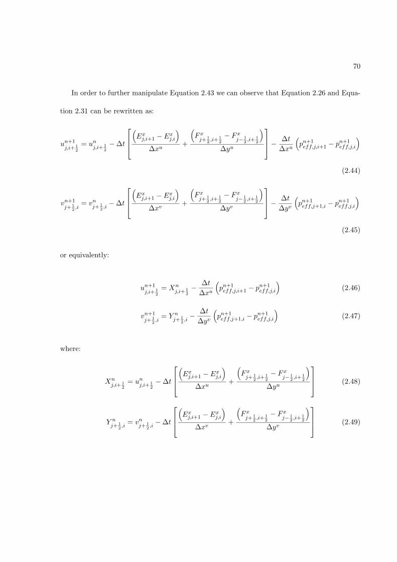
70

In order to further manipulate Equation 2.43 we can observe that Equation 2.26 and Equa-

tion 2.31 can be rewritten as:

un+1j,i+ 1

2

= unj,i+ 1

2

−∆t

(Exj,i+1 − Exj,i

)∆xu

+

(F xj+ 1

2,i+ 1

2

− F xj− 1

2,i+ 1

2

)∆yu

− ∆t

∆xu

(pn+1eff,j,i+1 − p

n+1eff,j,i

)

(2.44)

vn+1j+ 1

2,i

= vnj+ 1

2,i−∆t

(Exj,i+1 − Exj,i

)∆xv

+

(F xj+ 1

2,i+ 1

2

− F xj− 1

2,i+ 1

2

)∆yv

− ∆t

∆yv

(pn+1eff,j+1,i − p

n+1eff,j,i

)

(2.45)

or equivalently:

un+1j,i+ 1

2

= Xnj,i+ 1

2

− ∆t

∆xu

(pn+1eff,j,i+1 − p

n+1eff,j,i

)(2.46)

vn+1j+ 1

2,i

= Y nj+ 1

2,i− ∆t

∆yv

(pn+1eff,j+1,i − p

n+1eff,j,i

)(2.47)

where:

Xnj,i+ 1

2

= unj,i+ 1

2

−∆t

(Exj,i+1 − Exj,i

)∆xu

+

(F xj+ 1

2,i+ 1

2

− F xj− 1

2,i+ 1

2

)∆yu

(2.48)

Y nj+ 1

2,i

= vnj+ 1

2,i−∆t

(Exj,i+1 − Exj,i

)∆xv

+

(F xj+ 1

2,i+ 1

2

− F xj− 1

2,i+ 1

2

)∆yv

(2.49)

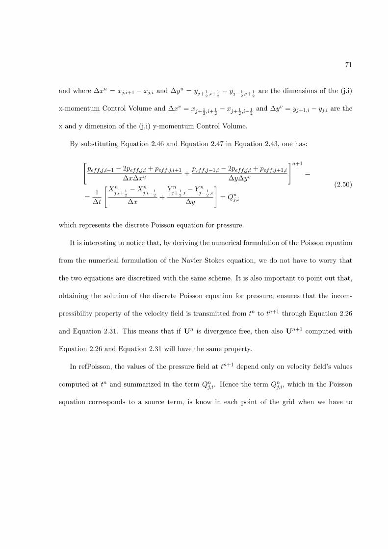
71

and where ∆xu = xj,i+1 − xj,i and ∆yu = yj+ 12,i+ 1

2− yj− 1

2,i+ 1

2are the dimensions of the (j,i)

x-momentum Control Volume and ∆xv = xj+ 12,i+ 1

2− xj+ 1

2,i− 1

2and ∆yv = yj+1,i − yj,i are the

x and y dimension of the (j,i) y-momentum Control Volume.

By substituting Equation 2.46 and Equation 2.47 in Equation 2.43, one has:

[peff,j,i−1 − 2peff,j,i + peff,j,i+1

∆x∆xu+peff,j−1,i − 2peff,j,i + peff,j+1,i

∆y∆yv

]n+1

=

=1

∆t

[Xnj,i+ 1

2

−Xnj,i− 1

2

∆x+Y nj+ 1

2,i− Y n

j− 12,i

∆y

]= Qnj,i

(2.50)

which represents the discrete Poisson equation for pressure.

It is interesting to notice that, by deriving the numerical formulation of the Poisson equation

from the numerical formulation of the Navier Stokes equation, we do not have to worry that

the two equations are discretized with the same scheme. It is also important to point out that,

obtaining the solution of the discrete Poisson equation for pressure, ensures that the incom-

pressibility property of the velocity field is transmitted from tn to tn+1 through Equation 2.26

and Equation 2.31. This means that if Un is divergence free, then also Un+1 computed with

Equation 2.26 and Equation 2.31 will have the same property.

In refPoisson, the values of the pressure field at tn+1 depend only on velocity field’s values

computed at tn and summarized in the term Qnj,i. Hence the term Qnj,i, which in the Poisson

equation corresponds to a source term, is know in each point of the grid when we have to

72

compute pn+1eff,j,i. The discrete equation (Equation 2.50) correspond to the discretization of the

Poisson equation for pressure:

∇2peff =∂2peff∂x2

+∂2peff∂y2

= f(x, y) (2.51)

where Qnj,i ≡ f(xi, yj).

In order to solve the discrete Poisson Equation 2.50, it is possible to transform Equation 2.51

into a transient problem, as shown in the following section.

2.1.9 Poisson Equation Solver

Equation 2.50 is solved using the Gauss-Seidel iterative method. Starting from the unsteady

Poisson equation for pressure and substituting P = peff for ease of writing, one has:

∂2P

∂x2+∂2P

∂y2= f(x, y) (2.52)

one can think of transforming it into a transient problem by looking for the steady state solution

of equation:

∂P

∂t=∂2P

∂x2+∂2P

∂y2− f(x, y) (2.53)

73

since at steady state∂P

∂t= 0. Hence the steady state solution of Equation 2.53 corresponds to

the solution of Equation 2.51.By applying a Finite Difference, Central-in-space and Forward-

in-time discretization to Equation 2.53, as shown above, one has:

Pn+1j,i − Pnj,i

∆t=Pnj,i−1 − 2Pnj,i + Pnj,i+1

∆x∆xu+Pnj−1,i − 2Pnj,i + Pnj+1,i

∆y∆yv−Qnj,i (2.54)

On a uniform grid with ∆ = ∆x = ∆y and choosing ∆t = ∆/4 which corresponds to the

maximum allowed ∆t due to stability reasons, it follows:

Pn+1i,j =

1

4

(Pni−1,j + Pni,j−1 + Pni+1,j + Pni,j+1 −∆2Qni,j

)(2.55)

which is the Richarson Method. In the case of non-uniform grid -as the one here - the derivation

is similar and straightforward, hence it will not be presented here.

The Gauss-Seidel method follows a similar derivation which leads to:

Pn+1i,j =

1

4

(Pn+1i−1,j + Pn+1

i,j−1 + Pni+1,j + Pni,j+1 −∆2Qni,j

)(2.56)

74

It is important to notice that Equation 2.56 is still an explicit method. Indeed, despite the

quantity Pn+1i−1,j + Pn+1

i,j−1 is involved, one can observe that the two values are already computed

before calculating Pn+1i,j . Applying a successive over-relaxation one obtains:

P̃n+1i,j = 1

4

(Pn+1i−1,j + Pn+1

i,j−1 + Pni+1,j + Pni,j+1 −∆2Qni,j

)

Pn+1i,j = Pni,j + ω(P̃n+1

i,j − Pni,j)

(2.57)

where ω is the relaxation factor. Here we chose ω = 1.6 as it is the optimal value that, for this

case, allows a fewer number of iterations to get to the steady-state solution. Again, equations

in system above are both explicit.

Hence, in order to solve Equation 2.50, one starts with a tentative pressure fields and

applies Equation 2.57 iteratively until the change between the pressure fields of two consecutive

iterations is below a certain tolerance. At this point, the pressure field will correspond to the

steady state solution of Equation 2.53 and therefore to the solution of Equation 2.51.

Once the pressure field has been calculated, the values of pressure can be used in Equa-

tion 2.26 and Equation 2.31 to compute the velocity field at the next time step. Since in general

the pressure field does not change a lot between two consecutive times steps ,as a good initial

value of the pressure field one should use the pressure distribution at the previous time step.

A final remark is that when Equation 2.57 is computed in correspondence of the boundary

cells, some indices will exceed the physical domain. In this case, the pressure boundary condi-

75

tions on the four walls must be used. These Boundary Conditions will be directly enforced on

the ghost cells’ layer as it will be explained in the following sections.

2.2 Turbulent fully-developed channel flow

Here we briefly review a few key concepts of the physics of turbulent channel flow, since it

is the flow case to whom the RANS solver will be applied. Turbulent channel flow is a pressure-

driven flow between two parallel planes where the fluid proceeds primarily along the x direction.

The direction normal to the wall is the y direction [12]. If we assume an infinite width of the

plates, so that any edge effect can be neglected, the flow results two-dimensional and can be

analyzed in the x-y plane only, as showed in Figure 14.When a pressure gradient dp/dx < 0 is

applied, the fluid accelerates in the x direction and the velocity profile U(y) assumes different

shapes along the plate lenght. In particular, a velocity boundary layer develops from the channel

inlet through the channel length. If the channel is sufficiently long, the velocity boundary layer

reaches the channel axis: at that point the flow is said to be fully developed since the velocity

profile remains steady and does not change anymore with x.

Therefore, a fully-developed, turbulent channel flow shows a one-dimensional structure along

the y direction. That is, after performing the averaging procedure, the flow quantities (such as

average velocity) are only functions of the distance across the channel, y.

It is natural to normalize the wall-normal distance y and to work in viscous wall units which

are denoted by:

y+ =y

hν(2.58)

76

where hν = ν/uτ is the viscous lengthscale and:

uτ =

√τwρ

(2.59)

is called the friction velocity, with τw being the shear stress at the wall.

Figure 14: Geometry of the channel flow

The dimensionless quantity:

Reτ =uτh

ν(2.60)

where h is half the height of the channel, is called the friction Reynolds number.

Lastly, a key turbulence nondimensionalization used in channel flows is [7] :

u+ =u

uτ(2.61)

77

Working with y+ units is a convenient normalization for wall-bounded flows, as it naturally

reveals important regions of the flow field. In channel flows, the near-wall and bulk regions

exhibit distinctly different flow features, with dissipation mostly localized within the former.

Many simple eddy viscosity models do not make any distinction between these regions and

therefore ad-hoc damping factors are used in low-Reynolds models - such as fµ for the Abe-

Kondoh-Nagano one [17].

In this present work, the turbulent channel flow at Reτ = 544 - corresponding to a Reb =

10000 [25] based on the bulk mean flow u - is used both as a validation case for the RANS

solver and as a test-case for the implementation of the proposed data driven approach. Indeed,

the channel flow was the first geometries for which a Direct Numerical Simulation has been

performed and therefore it represents a classical benchmark for testing CFD turbulent solvers.

In the simulations, the geometry consists only of half of the height of the channel due to

simmetry reasons. Moreover, only the fully developed region is simulated, both because most

of the validation DNS data are available for this region and in order to minimize the simulation

time.

Lastly, it is important to choose the characteristic length and velocities used to nondimen-

sionalize the main variables according to Equation 2.5. Using the same notation of Equation 2.5,

for the channel flow it has been chosen:

U = uτ L = h (2.62)

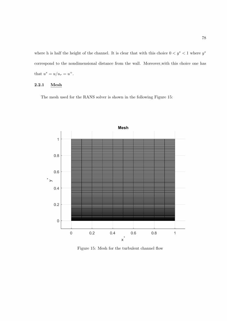
78

where h is half the height of the channel. It is clear that with this choice 0 < y∗ < 1 where y∗

correspond to the nondimensional distance from the wall. Moreover,with this choice one has

that u∗ = u/uτ = u+.

2.2.1 Mesh

The mesh used for the RANS solver is shown in the following Figure 15:

Figure 15: Mesh for the turbulent channel flow

79

whereas in Figure 16 it is shown a magnification of Figure 15 near the wall (y∗ = 0) to highlight

the near-wall resolution required by a wall resolved method.

Figure 16: Near-wall resolution of the mesh for the turbulent channel flow

The mesh consists of Ny = 120 cells along the y direction and Nx = 10 points along the x

direction. This choice is motivated by the fact that, in the fully developed region, the quantities

80

vary only with y and therefore the x direction is not relevant for the description of the flow. It

is also important to mention that the horizontal size of the mesh 0 < x∗ < 1 could have been

chosen differently, since the profile of the quantities is the same along x. The size value 1 was

chosen in order to obtain an easy value of ∆p∗ to compute, as later shown.

As far as the cell dimension is concerned, the following distribution has been chosen:

• ∆x is the same for all the cells, since the gradient of the quantities along the x direction

is null.

• For the vertical dimension a groth-rate type of stretching is chosen. This stretching along

y satisfies:

∆yi+1

∆yi= g = const (2.63)

where ∆yi is the vertical dimension of a generic cell, ∆yi+1 is the vertical dimension of

the cell above and g=1.02 is a constant. This stretching of the cell’s vertical dimension

is justified by the attempt to reduce the numerical discretization error. Indeed, when a

numerical approximation is introduced, like the one of the first derivative (Equation 2.21),

the difference between the real value of the discretized quantity and the value of its

numerical approximation is proportional to the gradient of the quantity and to the cell

size. Hence, the general idea driving a mesh realization is to refine it in regions where the

gradients of the quantities is steeper - in order to catch these steep variations - and to

make it coarser where the quantities are almost constant. Since in a a turbulent channel

flow the gradient of all quantities is very steep near the wall and null at the channel’s

81

centerline, it is a general practice to refine the mesh size near the wall and to have a

coarser mesh near the centerline, as the growth-rate relation above ensures.

Since a low-Reynolds model is employed, one has to ensure that the first cell falls well into the

viscous sublayer. The usual value is y+ ' 1.

From the definition of hν = ν/uτ , one has:

h∗ν =hνh

=ν

uτh=

1

Reτ(2.64)

from which:

y+∗ =y∗

h∗ν= y∗Reτ (2.65)

Hence y+ ' 1 will correspond, in nondimensional units, to:

∗ =1

Reτ= 0.00184 (2.66)

By using g=1.02 and Ny = 120, the first cell’s height corresponds to y∗ = 0.00175 ' 0.00184

and therefore the condition on the mesh wall resolution is satisfied.

2.2.2 Boundary Conditions

A scheme of the boundary conditions is presented in the Figure 17.At y∗ = 0 a wall boundary

condition is enforce to reproduce the presence of the physical wall. At y∗ = 1 a symmetry

boundary condition is enforce since this boundary corresponds to the channel axis and the

problem is symmetric with respect to it. At x∗ = 1 and x∗ = 0 a Zero Gradient boundary

82

condition is enforced because the flow is simulated in the fully-developed region, where the

variation of velocity and turbulent quantities along x is null.

Figure 17: Channel flow boundary conditions

Yet, it is important to stress that the Zero Gradient condition does not apply to pressure.

Indeed, pressure represents the ’driving force’ of the fluid, and to keep to fluid in motion along

83

the channel a negative pressure gradient dp/dx is necessary - Fig.(Figure 14). By manipulating

the axial mean-momentum equation (Equation 2.23) under the assumptions of boundary-layer

flow, and by recalling that uτ =√τw/ρ one has for the channel flow:

−dpdx

=τwh

=ρu2τh

(2.67)

where one can also demonstrate that the axial pressure gradient dp/dx is uniform across the

flow. By recalling the nondimensionalization (Equation 2.5), Equation (Equation 2.67) can be

rewritten as:

d

(p

ρu2τ

)d(x/h)

=dp∗

dx∗= −1 (2.68)

and, since the mean axial pressure gradient is uniform across the flow:

∆p∗ = p∗in − p∗out =

∫dx∗ = L∗ (2.69)

where L∗ is the length of the channel portion simulated - in this case L∗ = 1.

Another important aspect to mention is the ’relative’ nature of pressure in the Marker and

Cell method. Indeed, from the passages above, it emerges clearly that the computation of the

pressure field represents simply an intermediate step for the computation of the velocity field.

One can observe that Equation 2.51 yields infinite solutions when only one boundary condition

is specified, all of them differing for a constant [23].

84

Hence, unless the value of the actual pressure field is of interest, the solution of the Poisson

equation can be regarded as a ’pseudo-pressure’ field that leads to the solution of the real

velocity field. In Equation 2.26 and Equation 2.31, only the gradients of the ’pseudo-pressure’

field are involved, thus all the solutions of the Poisson equation produce the same effect on the

computation of the velocity components. As a consequence, the values of the pressure imposed

at the inlet and at the outle of the domain are not relevant, it is only their relation expressed

in Equation 2.69 that matters and that must be satisfied.

In order to enforce the boundary conditions sketched in Figure 17, it is convenient to define

an additional layer of cells outside the physical domain. We will refer to those control volumes

as ghost cells. The velocity components u and v, the pressure and the turbulence quantities

in correspondence of the ghost cell will be computed by directly enforcing the corresponding

boundary conditions, as it will be explained in the following section. Another possibility would

consist in modifying Equation 2.26, Equation 2.31, Equation 2.36 and Equation 2.41 in corre-

spondence of the boundary cells through the relations derived by the boundary conditions. It

is however much easier to extend the computational domain of one layer of cells and to use the

same expressions for each cell of the internal grid. A simplified scheme -with uniform cells - of

the resulting grid is sketched in the Figure 18, where the ghost cell layer is drawn with the red

color.

In the following paragraphs, a detailed explanation of the four boundary conditions will be

presented. Since U = (u, v) is a two-dimensional vector, the boundary conditions have to be

85

Figure 18: Ghost cells

specified for: each component of the velocity vector; the pressure; the turbulent kinetic energy;

the dissipation rate; the components of the anisotropy stress tensor.

2.2.2.1 Wall boundary condition y∗ = 0

First of all, we need to derive the continous boundary conditions for all the quantities in-

volved. After that, these expressions will be discretized so that they can be enforced numerically

in the solver.

In correspondence of a wall, the velocity boundary conditions derive from the no-slip and

the no-compenetration condition. In particular, the first one implies that, in correspondence of

each wall, the fluid velocity’s component parallel to the wall must be equal to the velocity of

the wall itself (in this case 0). The second one implies that, in correspondence of each wall, the

86

flow velocity’s component normal to the wall must be null, since no outgoing or entering mass

flow rate is allowed by the solid boundary.

From the no-slip condition and from the impermeability condition, it is also possible to

demonstrate that, in correspondence of a physical wall boundary, all the components of the

Reynolds stress tensor are null. In particular, one has that for y∗ → 0:

〈u2〉 ∼ y2

〈v2〉 ∼ y4

〈w2〉 ∼ y2

〈uv〉 ∼ y3

(2.70)

and therefore for y∗ = 0 all the anisotropy stress tensor components satisfy aij(y∗ = 0) = 0.

Moreover, since the turbulent kinetic energy, corresponds to half of the trace of the Reynolds

stress tensor, then also k(y∗ = 0) = 0.

Lastly, from the prescriptions of the Abe-Kondoh-Nagano model, one has:

ε(y = 0) = 2ν

(∂k

∂y

)2

y=0

(2.71)

which differs from the dissipation rate boundary condition that would normally derive by the

k transport equation:

ε(y = 0) = νd2k

dy2(2.72)

87

due to the introduction of the blending coefficients f1 and f2 in the ε transport equation, that

affect the expression near the wall.

The boundary conditions on pressure are derived from the Momentum Equations in corre-

spondence of the four walls and by combining the velocity boundary conditions.

The Momentum equation along y of the Navier-Stokes system written in non-conservative

form is:

∂v

∂t+ u

∂v

∂x+ v

∂v

∂y+

1

ρ

∂p

∂y+

2

3

∂k

∂y= ν

(∂2v

∂x2+∂2v

∂y2

)−(∂axy∂x− ∂ayy

∂y

)(2.73)

Yet, in correspondence of the horizontal bottom wall v=0,∂v

∂x= 0, aij = 0, k=0. Hence

Equation 2.73 becomes for the y=0 wall:

∂p

∂y= ρν

∂2v

∂y2= µ

∂2v

∂y2(2.74)

It is interesting to notice that the boundary condition for the pressure involves the velocity field

as well.

88

Now, by recalling all the reasoning above, the bottom wall boundary condition at y∗ = 0

can be expressed as:

u = 0

v = 0

∂p

∂y= µ

∂2v

∂y2

k = 0

aij = 0

ε = 2ν

(∂k

∂y

)2

y=0

(2.75)

By introducing the nondimensionalization parameters derived in Equation 2.5, the set of

boundary conditions (Equation 2.75) can be nondimensionalized as follows:

u∗ = 0

v∗ = 0

∂p∗

∂y∗=

1

Re

∂2v∗

∂y∗2

k∗ = 0

a∗ij = 0

ε∗ =2

Re

(∂k∗

∂y∗

)2

y∗=0

(2.76)

Equation 2.76 correspond to the nondimensional boundary conditions on the bottom wall. As

mentioned earlier, the boundary conditions are enforced by adding an extra layer of ghost cells.

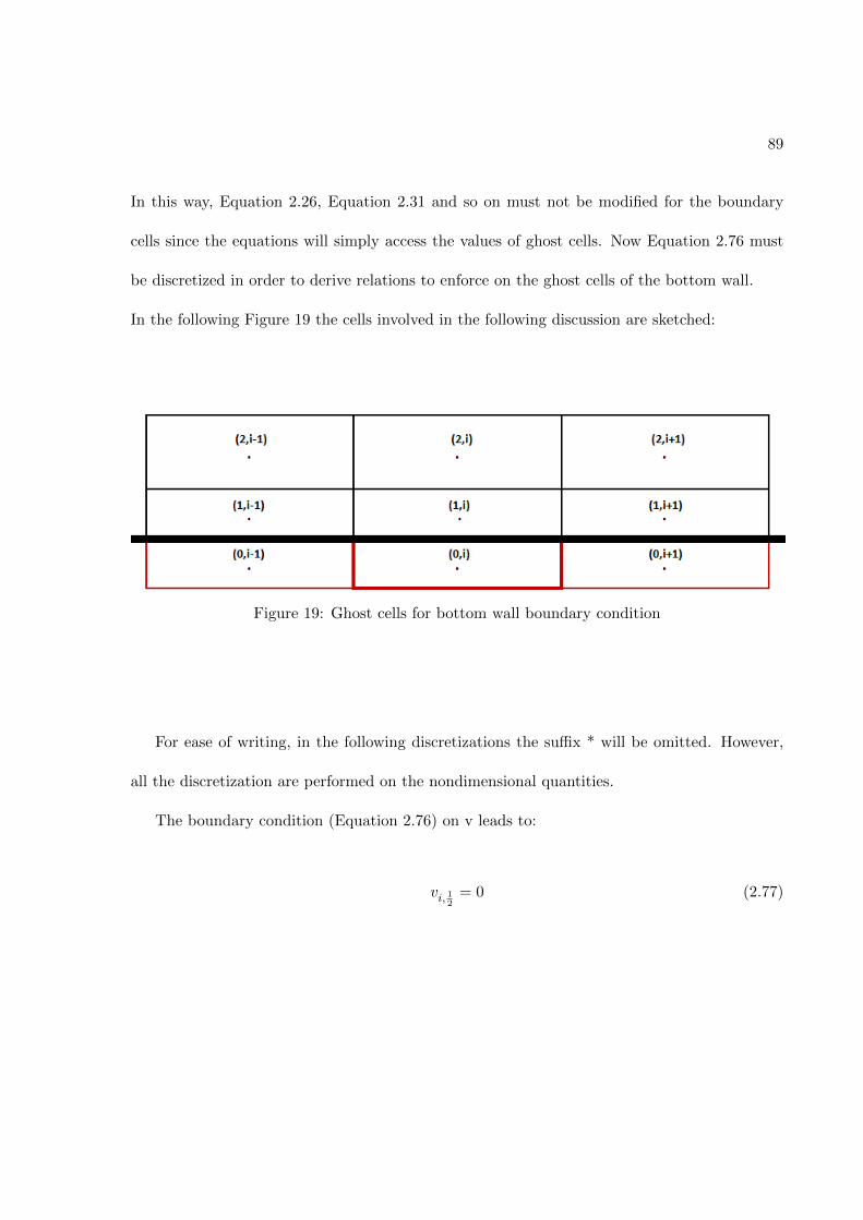
89

In this way, Equation 2.26, Equation 2.31 and so on must not be modified for the boundary

cells since the equations will simply access the values of ghost cells. Now Equation 2.76 must

be discretized in order to derive relations to enforce on the ghost cells of the bottom wall.

In the following Figure 19 the cells involved in the following discussion are sketched:

Figure 19: Ghost cells for bottom wall boundary condition

For ease of writing, in the following discretizations the suffix * will be omitted. However,

all the discretization are performed on the nondimensional quantities.

The boundary condition (Equation 2.76) on v leads to:

vi, 12

= 0 (2.77)

90

From a simple interpolation, the boundary condition (Equation 2.75) on u leads to:

uwall,i+ 12

=ui+ 1

2,0 + ui+ 1

2,1

2(2.78)

from which for the ghost cell:

ui+ 12,0 = 2uwall,i+ 1

2− ui+ 1

2,1 = −ui+ 1

2,1 (2.79)

For the pressure instead, by recalling the continuity equation of (Equation 2.1) one has:

∂p

∂y=

1

Re

∂2v

∂y2=

1

Re

∂

∂y

(∂v

∂y

)=

1

Re

∂

∂y

(−∂u∂x

)= − 1

Re

∂

∂x

(∂u

∂y

)(2.80)

from which: [∂p

∂y= − 1

Re

∂

∂x

(∂u

∂y

)]i, 1

2

(2.81)

By discretizing the equation above in correspondence of the wall with a Central-Space

scheme one obtains:

pi,1 − pi,0∆y

= − 1

Re

(∂u∂y

)i+ 1

2, 12

−(∂u∂y

)i− 1

2, 12

∆x= − 1

Re

(ui+ 1

2,1 − ui+ 1

2,0

)−(ui− 1

2,1 − ui− 1

2,0

)∆x∆y

(2.82)

and applying the Boundary Condition on u mentioned above:

pi,1 − pi,0∆y

= − 2

Re

ui+ 12,1 − ui− 1

2,1

∆x∆y+

2

Re

uwall,i+ 12− uwall,i− 1

2

∆x∆y(2.83)

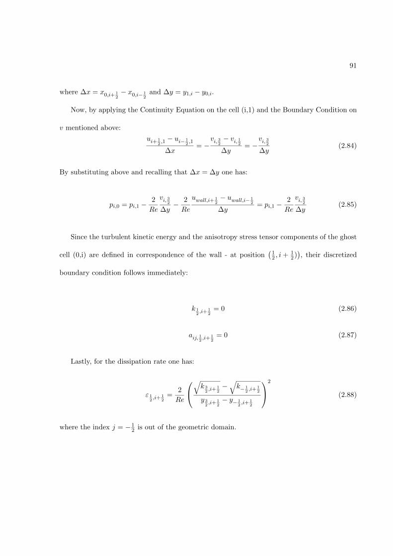
91

where ∆x = x0,i+ 12− x0,i− 1

2and ∆y = y1,i − y0,i.

Now, by applying the Continuity Equation on the cell (i,1) and the Boundary Condition on

v mentioned above:

ui+ 12,1 − ui− 1

2,1

∆x= −

vi, 32− vi, 1

2

∆y= −

vi, 32

∆y(2.84)

By substituting above and recalling that ∆x = ∆y one has:

pi,0 = pi,1 −2

Re

vi, 32

∆y− 2

Re

uwall,i+ 12− uwall,i− 1

2

∆y= pi,1 −

2

Re

vi, 32

∆y(2.85)

Since the turbulent kinetic energy and the anisotropy stress tensor components of the ghost

cell (0,i) are defined in correspondence of the wall - at position(12 , i+ 1

2)), their discretized

boundary condition follows immediately:

k 12,i+ 1

2= 0 (2.86)

aij, 12,i+ 1

2= 0 (2.87)

Lastly, for the dissipation rate one has:

ε 12,i+ 1

2=

2

Re

√k 3

2,i+ 1

2−√k− 1

2,i+ 1

2

y 32,i+ 1

2− y− 1

2,i+ 1

2

2

(2.88)

where the index j = −12 is out of the geometric domain.

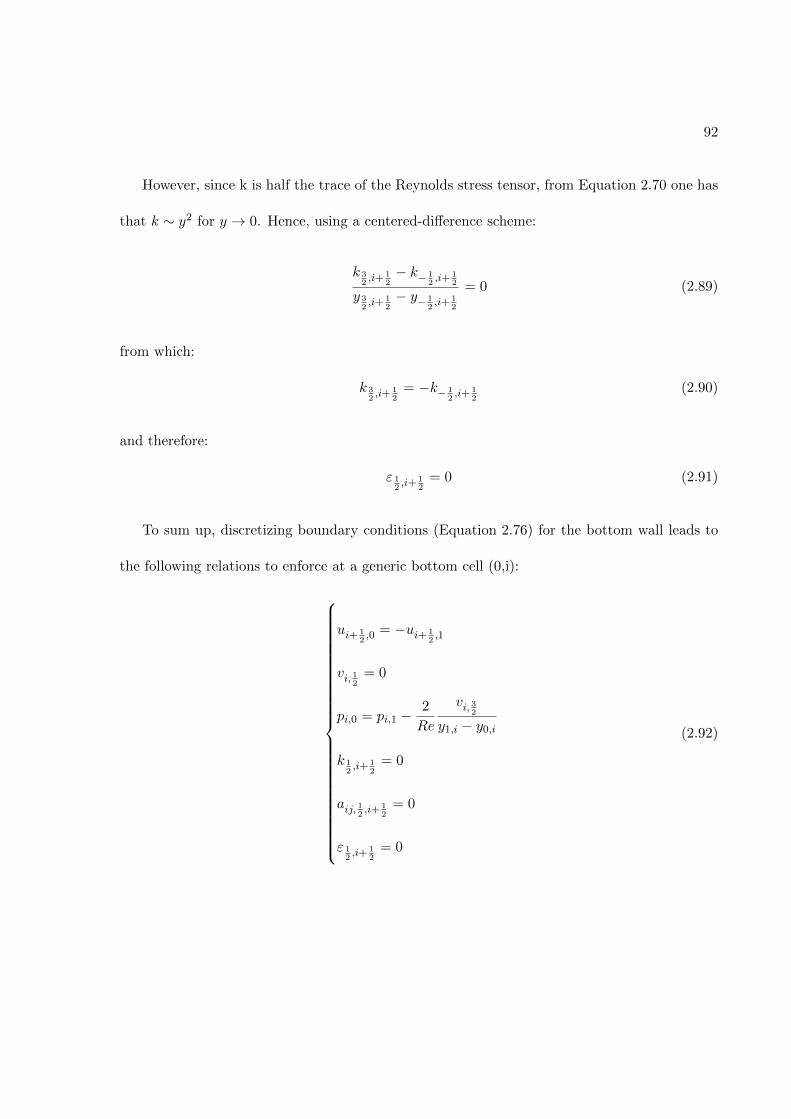
92

However, since k is half the trace of the Reynolds stress tensor, from Equation 2.70 one has

that k ∼ y2 for y → 0. Hence, using a centered-difference scheme:

k 32,i+ 1

2− k− 1

2,i+ 1

2

y 32,i+ 1

2− y− 1

2,i+ 1

2

= 0 (2.89)

from which:

k 32,i+ 1

2= −k− 1

2,i+ 1

2(2.90)

and therefore:

ε 12,i+ 1

2= 0 (2.91)

To sum up, discretizing boundary conditions (Equation 2.76) for the bottom wall leads to

the following relations to enforce at a generic bottom cell (0,i):

ui+ 12,0 = −ui+ 1

2,1

vi, 12

= 0

pi,0 = pi,1 −2

Re

vi, 32

y1,i − y0,i

k 12,i+ 1

2= 0

aij, 12,i+ 1

2= 0

ε 12,i+ 1

2= 0

(2.92)

93

2.2.2.2 Symmetry boundary condition y∗ = 1

As before, first the continuous boundary conditions will be derived for all the quantities and,

after that, the expressions will be discretized for the layer of ghost cells. In correspondence

of the channel axis, the profile of all the quantities are specular due to the symmetry of the

problem. Mathematically, this constraint translates into a zero-gradient condition for all the

variables, except the component v of the velocity which is normal to the channel axis. Again,

due to the symmetry of the problem, the component of velocity normal to the simmetry axis

-here v- must be null.

Recalling the reasoning above, the top symmetry boundary condition at y∗ = 1 can be

expressed as:

∂u

∂y= 0

v = 0

∂p

∂y= 0

∂k

∂y= 0

∂aij∂y

= 0

∂ε

∂y= 0

(2.93)

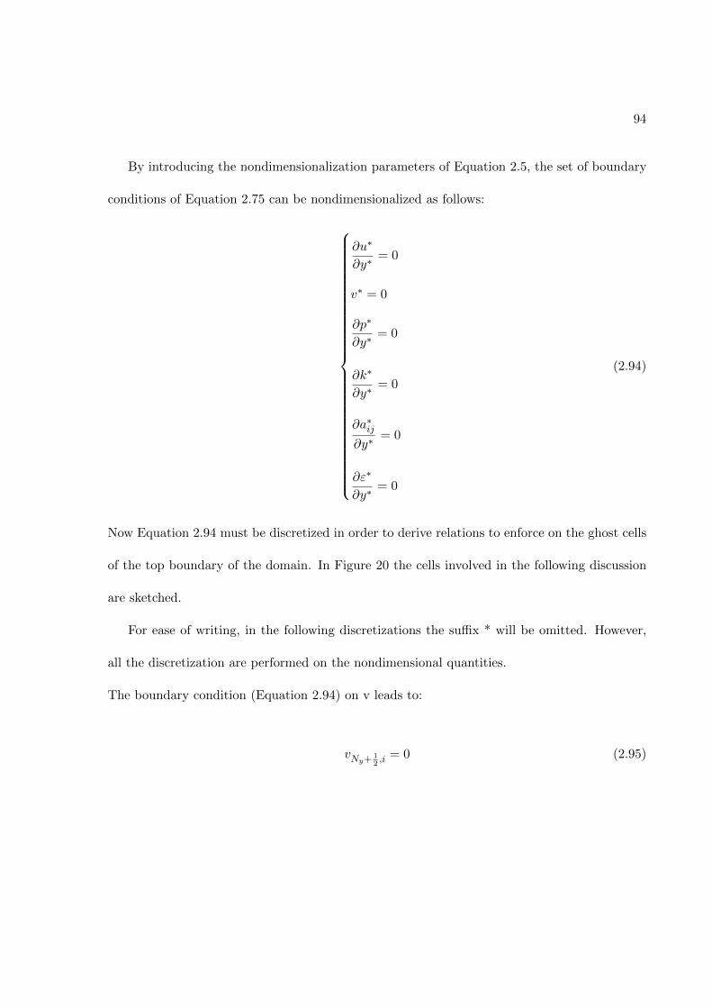
94

By introducing the nondimensionalization parameters of Equation 2.5, the set of boundary

conditions of Equation 2.75 can be nondimensionalized as follows:

∂u∗

∂y∗= 0

v∗ = 0

∂p∗

∂y∗= 0

∂k∗

∂y∗= 0

∂a∗ij∂y∗

= 0

∂ε∗

∂y∗= 0

(2.94)

Now Equation 2.94 must be discretized in order to derive relations to enforce on the ghost cells

of the top boundary of the domain. In Figure 20 the cells involved in the following discussion

are sketched.

For ease of writing, in the following discretizations the suffix * will be omitted. However,

all the discretization are performed on the nondimensional quantities.

The boundary condition (Equation 2.94) on v leads to:

vNy+12,i = 0 (2.95)

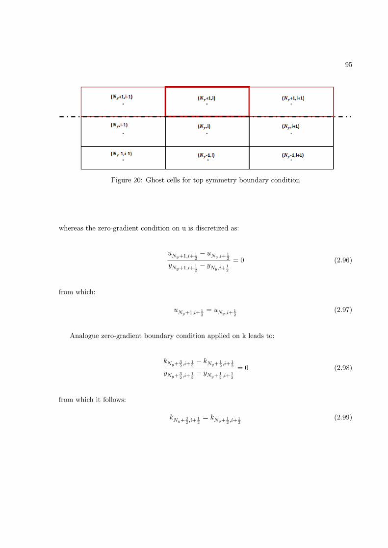
95

Figure 20: Ghost cells for top symmetry boundary condition

whereas the zero-gradient condition on u is discretized as:

uNy+1,i+ 12− uNy ,i+

12

yNy+1,i+ 12− yNy ,i+

12

= 0 (2.96)

from which:

uNy+1,i+ 12

= uNy ,i+12

(2.97)

Analogue zero-gradient boundary condition applied on k leads to:

kNy+32,i+ 1

2− kNy+

12,i+ 1

2

yNy+32,i+ 1

2− yNy+

12,i+ 1

2

= 0 (2.98)

from which it follows:

kNy+32,i+ 1

2= kNy+

12,i+ 1

2(2.99)

96

A similar condition to the one above applies to ε and aij , since like k they are defined at

the cell vertex. Lastly, the zero-gradient condition applied to the pressure leads to:

pNy+1,i = pNy ,i (2.100)

To sum up, discretizing boundary conditions expressed in Equation 2.94 for the top boundary

leads to the following relations to enforce at a generic ghost cell (Ny + 1, i):

uNy+1,i+ 12

= uNy ,i+12

vNy+12,i = 0

pNy+1,i = pNy ,i

kNy+32,i+ 1

2= kNy+

12,i+ 1

2

aij,Ny+32,i+ 1

2= aij,Ny+

12,i+ 1

2

εNy+32,i+ 1

2= εNy+

12,i+ 1

2

(2.101)

2.2.2.3 Zero-gradient boundary condition x∗ = 0

As before, first the continuous boundary conditions will be derived for all the quantities and,

after that, the expressions will be discretized for the layer of ghost cells. In correspondence

of the inlet boundary of the domain a zero-gradient boundary condition is applied to all the

variables except the pressure. Indeed, the flow is simulated in the fully developed region in

which the quantities do not vary along the axial direction, their gradient along x being null.

97

The pressure represents the only variable with a non null variation along x since a negative

pressure gradient dp/dx is necessary to drive the flow in the channel.

As for the inlet value of the pressure pin = px=0, the relative nature of the pressure has

already been discussed above. Since only the gradient of the pressure field affect the computa-

tion of u and v - (Equation 2.26), (Equation 2.31) - then the actual value of the pressure pin

is irrelevant. What really matters is that the pressure at the inlet and the one at the outlet

satisfy (Equation 2.69).

Recalling the reasoning above, the left zero-gradient condition at x∗ = 0 can be expressed

as:

∂u

∂x= 0

∂v

∂x= 0

p = pin

∂k

∂x= 0

∂aij∂x

= 0

∂ε

∂x= 0

(2.102)

98

where the value of pin can be chosen arbitrarily. By introducing the nondimensionalization

parameters of Equation 2.5, the set of boundary conditions in Equation 2.75 can be nondimen-

sionalized as follows:

∂u∗

∂x∗= 0

∂v∗

∂x∗= 0

p∗ = p∗in

∂k∗

∂x∗= 0

∂a∗ij∂x∗

= 0

∂ε∗

∂x∗= 0

(2.103)

Now (Equation 2.103) must be discretized in order to derive relations to enforce on the

ghost cells of the left inlet boundary of the domain.In the following Figure 21 the cells involved

in the following discussion are sketched.

For ease of writing, in the following discretizations the suffix * will be omitted. However,

all the discretization are performed on the nondimensional quantities.

The boundary condition (Equation 2.103) on u leads to:

uj, 32− uj, 1

2

xj, 32− xj, 1

2

= 0 (2.104)

99

Figure 21: Ghost cells for left zero-gradient boundary condition

from which:

uj, 12

= uj, 32

(2.105)

Similarly, for the v component of velocity one has:

vj+ 12,0 = vj+ 1

2,1 (2.106)

Analogue zero-gradient boundary condition applied on k leads to:

kj+ 12, 32− kj+ 1

2, 12

xj+ 12, 32− xj+ 1

2, 12

= 0 (2.107)

from which it follows:

kj+ 12, 32

= kj+ 12, 12

(2.108)

100

A similar condition to the one above applies to ε and aij , since like k they are defined at

the cell vertex. Lastly, the inlet boundary condition applied to the pressure leads to:

pNy+1,i = pin (2.109)

To sum up, discretizing boundary conditions (Equation 2.94) for the top boundary leads to the

following relations to enforce at a generic ghost cell (j, 0):

uj, 12

= uj, 32

vj+ 12,0 = vj+ 1

2,1

pNy+1,i = pin

kj+ 12, 32

= kj+ 12, 12

aij,j+ 12, 32

= aij,j+ 12, 12

εj+ 12, 32

= εj+ 12, 12

(2.110)

2.2.2.4 Zero-gradient boundary condition x∗ = 1

For the right boundary of the domain at x∗ = 1, the boundary condition is analogue to

the one enforced at x∗ = 0 boundary. In correspondence of the outlet boundary of the domain

a zero-gradient boundary condition is applied to all the variables except the pressure, which

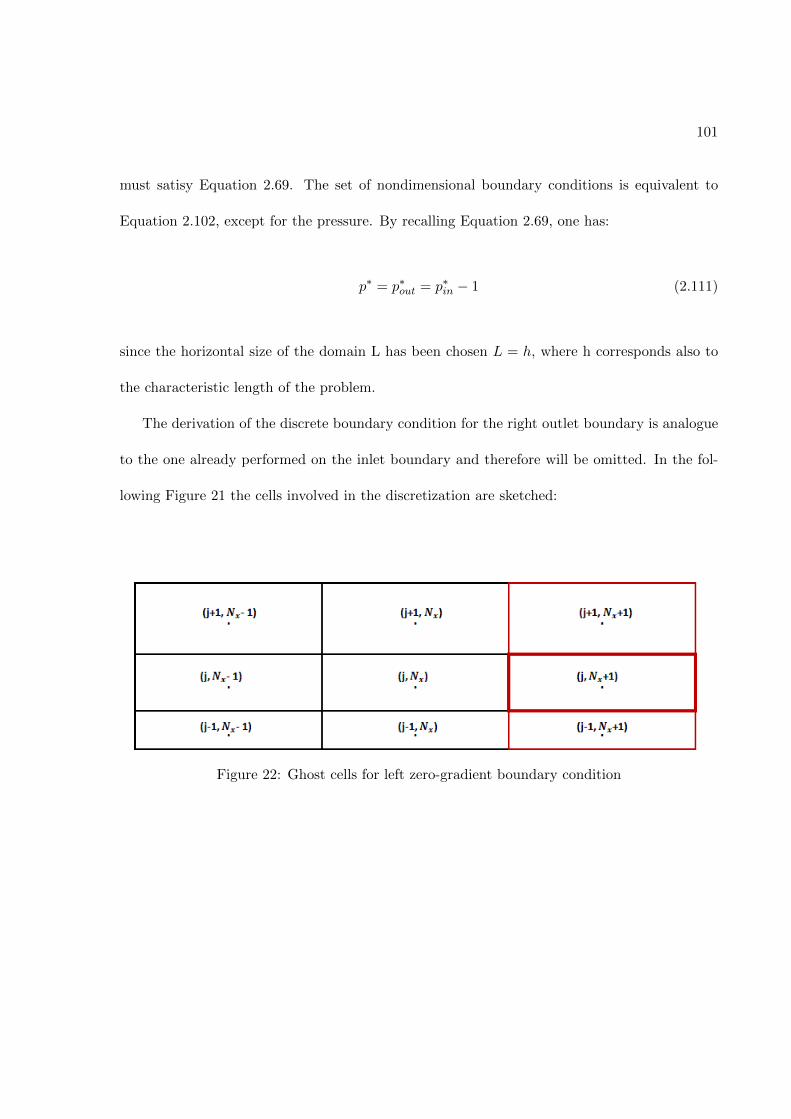
101

must satisy Equation 2.69. The set of nondimensional boundary conditions is equivalent to

Equation 2.102, except for the pressure. By recalling Equation 2.69, one has:

p∗ = p∗out = p∗in − 1 (2.111)

since the horizontal size of the domain L has been chosen L = h, where h corresponds also to

the characteristic length of the problem.

The derivation of the discrete boundary condition for the right outlet boundary is analogue

to the one already performed on the inlet boundary and therefore will be omitted. In the fol-

lowing Figure 21 the cells involved in the discretization are sketched:

Figure 22: Ghost cells for left zero-gradient boundary condition

102

The discretization of the continous outlet zero-gradient boundary condition on the rigth bound-

ary of the domain leads to the following conditions to enforce at generic ghost cell (j,Nx + 1):

uj,Nx+32

= uj,Nx+12

vj+ 12,Nx

= vj+ 12,Nx+1

pNy+1,i = pin − 1

kj+ 12,Nx+

32

= kj+ 12,Nx+

12

aij,j+ 12,Nx+

32

= aij,j+ 12,Nx+

12

ε 12,Nx+

32

= εj+ 12,Nx+

12

(2.112)

2.2.3 Validation of the solver

Before trying to embed a neural network, it has to be ensured that the standard version of

the solver -the one using the Linear Eddy Viscosity Model- yields satisfactory results.

The validation case chosen is the turbulent channel flow at Reτ = 544 or equivalently

Reδ = 10000. The choiche was motivated by the following facts:

• The application of the neural network will be tested on the same flow, hence the code can

be reused by just replacing the LEVM with the machine learning architecture.

• The turbulent channel flow is a canonical flow which has been extensively studied numeri-

cally. Indeed, it is the first class of flows to which DNS methods were applied. As a result,

it has been used for long time as a benchmark problem to test and validate numerical

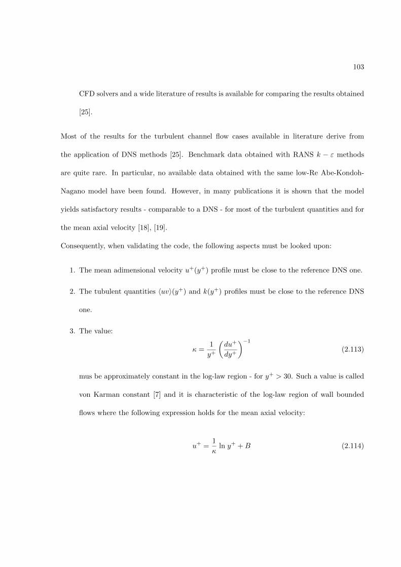
103

CFD solvers and a wide literature of results is available for comparing the results obtained

[25].

Most of the results for the turbulent channel flow cases available in literature derive from

the application of DNS methods [25]. Benchmark data obtained with RANS k − ε methods

are quite rare. In particular, no available data obtained with the same low-Re Abe-Kondoh-

Nagano model have been found. However, in many publications it is shown that the model

yields satisfactory results - comparable to a DNS - for most of the turbulent quantities and for

the mean axial velocity [18], [19].

Consequently, when validating the code, the following aspects must be looked upon:

1. The mean adimensional velocity u+(y+) profile must be close to the reference DNS one.

2. The tubulent quantities 〈uv〉(y+) and k(y+) profiles must be close to the reference DNS

one.

3. The value:

κ =1

y+

(du+

dy+

)−1(2.113)

mus be approximately constant in the log-law region - for y+ > 30. Such a value is called

von Karman constant [7] and it is characteristic of the log-law region of wall bounded

flows where the following expression holds for the mean axial velocity:

u+ =1

κln y+ +B (2.114)

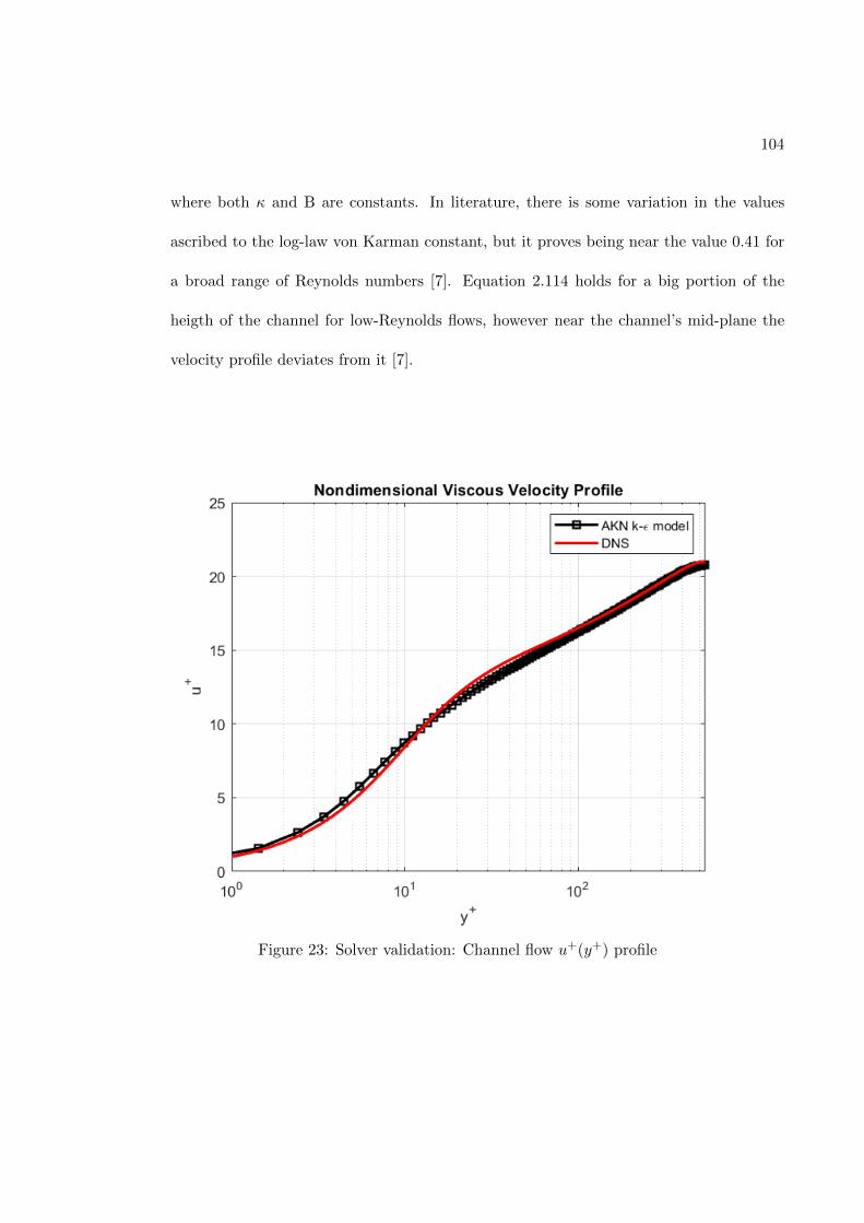
104

where both κ and B are constants. In literature, there is some variation in the values

ascribed to the log-law von Karman constant, but it proves being near the value 0.41 for

a broad range of Reynolds numbers [7]. Equation 2.114 holds for a big portion of the

heigth of the channel for low-Reynolds flows, however near the channel’s mid-plane the

velocity profile deviates from it [7].

Figure 23: Solver validation: Channel flow u+(y+) profile

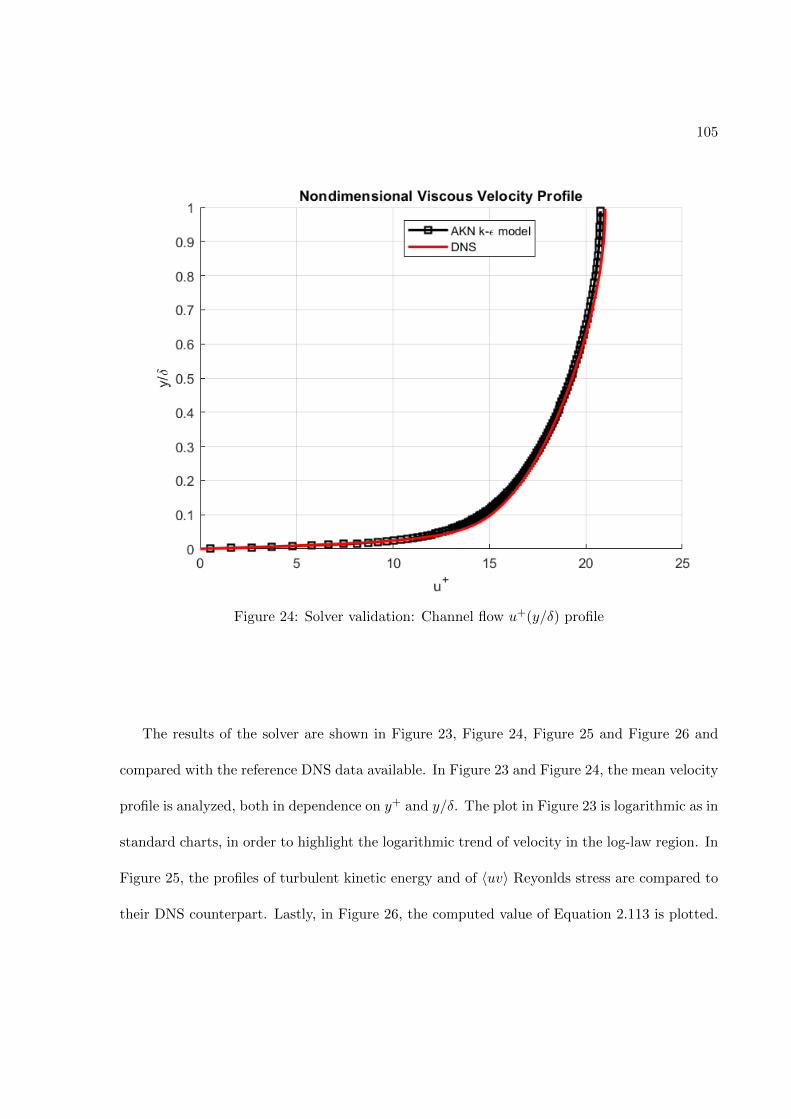
105

Figure 24: Solver validation: Channel flow u+(y/δ) profile

The results of the solver are shown in Figure 23, Figure 24, Figure 25 and Figure 26 and

compared with the reference DNS data available. In Figure 23 and Figure 24, the mean velocity

profile is analyzed, both in dependence on y+ and y/δ. The plot in Figure 23 is logarithmic as in

standard charts, in order to highlight the logarithmic trend of velocity in the log-law region. In

Figure 25, the profiles of turbulent kinetic energy and of 〈uv〉 Reyonlds stress are compared to

their DNS counterpart. Lastly, in Figure 26, the computed value of Equation 2.113 is plotted.

106

Figure 25: Solver validation: Channel flow k+(y+) and 〈uv(y+) profiles

From the charts presented, we can observe that the results obtained are fully satisfactory.

Indeed:

• The solver gives an acceptable prediction of the axial velocity profile. One must also

consider that the benchmark data derive from a DNS and therefore a small discrepancy

between them and the RANS results obtained is to be expected.

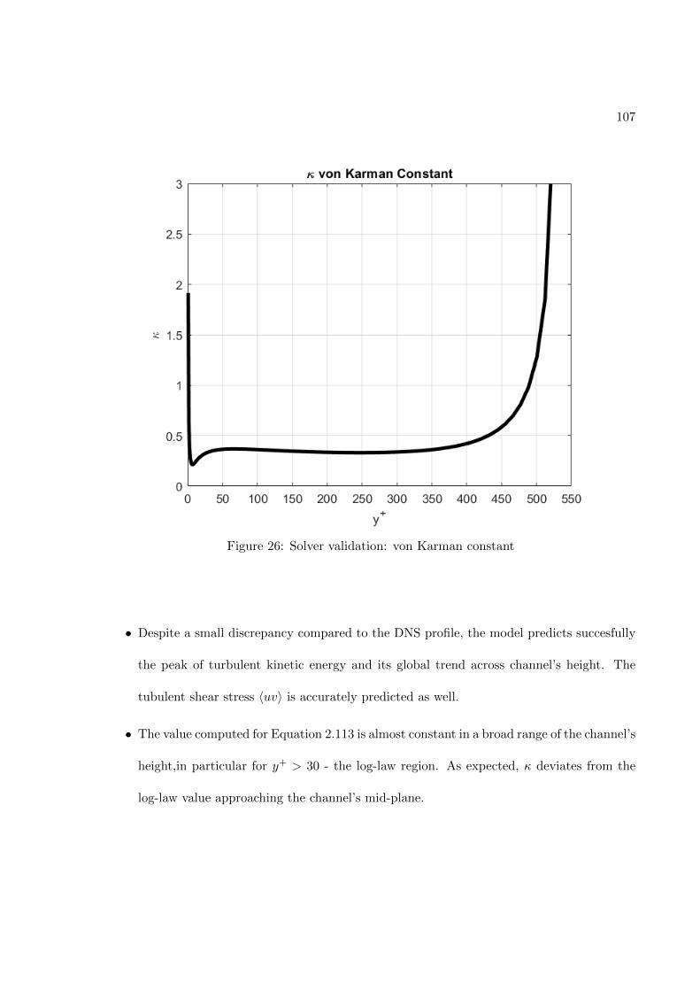
107

Figure 26: Solver validation: von Karman constant

• Despite a small discrepancy compared to the DNS profile, the model predicts succesfully

the peak of turbulent kinetic energy and its global trend across channel’s height. The

tubulent shear stress 〈uv〉 is accurately predicted as well.

• The value computed for Equation 2.113 is almost constant in a broad range of the channel’s

height,in particular for y+ > 30 - the log-law region. As expected, κ deviates from the

log-law value approaching the channel’s mid-plane.

108

2.3 Artificial Neural Network

In this section, further details will be given about the building and training of the Tensor

Basis Neural Network used to replace the LEVM in the solver. The network introduced in

Chapter 1 has been implemented in Python, using Keras library [26] with Tensorflow backend.

The choice is motivated by the fact that the network has a very standard layers’ architecture

(feed-forward, fully connected) and Keras provides many tools to easily build canonical net-

works. Moreover, at the time of the work, Tensorflow is among the most used libraries for

machine learning techniques.

In Table I the key terminology of neural networks is introduced.

2.3.1 High-Fidelity datasets

With the terminology introduced below, we are now ready to introduce the deep neural

network described in Chapter 1. The Tensor Basis Neural Network (TBNN) has two input

layers: the five invariants input layers -main input - and the ten basis tensors input layers.

A series of hydden layers is used to predicts coefficient g(n) for n=1,..10 of (Equation 1.36).

The tensor basis input layer is composed by the 10 invariant tensors T(n) for n=1,..10 of

Equation 1.36 from the five invariants λi. The merge output layer takes the element-wise

products of the final hidden layer and of the basis tensors input layer and sums the results to

give the final prediction for b [8] - which is the same as taking the dot product between the two

layers. All the quantities mentioned - the five invariants, the tensor basis, the nondimensional

anisotropy tensor - are derived from DNS or highly resolved LES datasets.

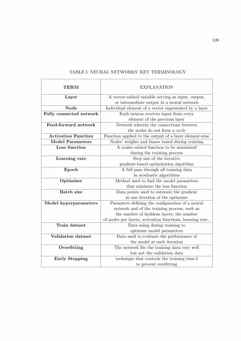
109

TABLE I: NEURAL NETWORKS’ KEY TERMINOLOGY

TERM EXPLANATION

Layer A vector-valued variable serving as input, output,or intermediate output in a neural network

Node Individual element of a vector represented by a layer

Fully connected network Each neuron receives input from everyelement of the previous layer

Feed-forward network Network wherein the connections betweenthe nodes do not form a cycle

Activation Function Function applied to the output of a layer element-wise

Model Parameters Nodes’ weights and biases tuned during training

Loss function A scalar-valued function to be minimizedduring the training process

Learning rate Step size of the iterativegradient-based optimization algorithm

Epoch A full pass through all training datain stochastic algorithms

Optimizer Method used to find the model parametersthat minimize the loss function

Batch size Data points used to estimate the gradientin one iteration of the optimizer

Model hyperparameters Paramters defining the configuration of a neuralnetwork and of the training process, such asthe number of hyddens layers, the number

of nodes per layers, activation functions, learning rate..

Train dataset Data using during training tooptimize model parameters

Validation dataset Data used to evaluate the performance ofthe model at each iteration

Overfitting The network fits the training data very wellbut not the validation data

Early Stopping technique that controls the training time ito prevent overfitting

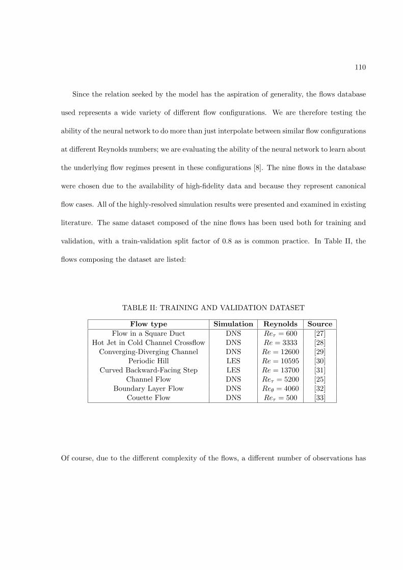
110

Since the relation seeked by the model has the aspiration of generality, the flows database

used represents a wide variety of different flow configurations. We are therefore testing the

ability of the neural network to do more than just interpolate between similar flow configurations

at different Reynolds numbers; we are evaluating the ability of the neural network to learn about

the underlying flow regimes present in these configurations [8]. The nine flows in the database

were chosen due to the availability of high-fidelity data and because they represent canonical

flow cases. All of the highly-resolved simulation results were presented and examined in existing

literature. The same dataset composed of the nine flows has been used both for training and

validation, with a train-validation split factor of 0.8 as is common practice. In Table II, the

flows composing the dataset are listed:

TABLE II: TRAINING AND VALIDATION DATASET

Flow type Simulation Reynolds Source

Flow in a Square Duct DNS Reτ = 600 [27]Hot Jet in Cold Channel Crossflow DNS Re = 3333 [28]

Converging-Diverging Channel DNS Re = 12600 [29]Periodic Hill LES Re = 10595 [30]

Curved Backward-Facing Step LES Re = 13700 [31]Channel Flow DNS Reτ = 5200 [25]

Boundary Layer Flow DNS Reθ = 4060 [32]Couette Flow DNS Reτ = 500 [33]

Of course, due to the different complexity of the flows, a different number of observations has

111

been used for each class of flows depending on the available data. For example, in the channel

flow case there is only one direction along which the quantities vary - the one normal to the

plates - and therefore only around 750 different points with different values were available. On

the other side, the Hot Jet in Cold Channel Crossflow is a 3D simulation (actually all DNS

simulations are 3D but in some cases the variation of the statistics occurs only along one or two

directions) and therefore many more data points were included in the dataset - around 160000.

2.3.2 Input layers’ normalizations

The data listed in Table Table II were not directly inputed into the neural network. Indeed,

it is an usual practice in machine learning algorithms to perfom a data normalization first when

features may have different ranges of values [34].

As mentioned above,in order to obtain nondimensional inputs, the normalization ot the

mean rate of strain 〈S〉 (Equation 1.32) and of the rate of rotation 〈R〉 (Equation 1.33) tensors

proposed by Pope is adopted. In this way, all raw features are normalized by local quantities,

as usual in the practice of traditional turbulence modeling [1]. Now, since all components of

112

the nondimensional Reynolds stress tensor lie in the range [−1/2,2/3], [7] the basis tensors have

been normalized in the following way:

T̃(1)

=1

a[〈s〉] =

1

aT(1)

T̃(2)

=1

ab[〈s〉〈r〉 − 〈r〉〈s〉] =

1

abT(2)

T̃(3)

=1

a2

[〈s〉2 − 1

3I · Tr

(〈s〉2

)]=

1

a2T(3)

T̃(4)

=1

b2

[〈r〉2 − 1

3I · Tr

(〈r〉2

)]=

1

b2T(4)

T̃(5)

=1

a2b

[〈r〉〈s〉2 − 〈s〉2〈r〉

]=

1

a2bT(5)

T̃(6)

=1

ab2

[〈r〉2〈s〉+ 〈r〉〈s〉2 − 2

3I · Tr

(〈s〉〈r〉2

)]=

1

ab2T(6)

T̃(7)

=1

ab3[〈r〉〈s〉〈r〉2 − 〈r〉2〈s〉〈r〉

]=

1

ab3T(7)

T̃(8)

=1

a3b

[〈s〉〈r〉〈s〉2 − 〈s〉2〈r〉〈s〉

]=

1

a3bT(8)

T̃(9)

=1

a2b2

[〈r〉2〈s〉2 − 〈s〉2〈r〉2 − 2

3I · Tr

(〈s〉2〈r〉2

)]=

1

a2b2T(9)

T̃(10)

=1

a2b3[〈r〉〈s〉2〈r〉2 − 〈r〉2〈s〉2〈r〉

]=

1

a2b3T(10)

where:

a =

√|Tr(〈s〉2)|

2b =

√|Tr(〈r〉2)|

2(2.115)

and where T̃(n)

refers to basis tensor T(n) normalized through Equation 2.115.

113

In order to justify the normalization described above, it is useful to provide an example

with a generic 2D nondimensional mean strain rate tensor:

〈s〉2D =

s11 s12 0

s21 s22 0

0 0 0

(2.116)

where s12 = s21 due to simmetry and the zeros are due to the fact that in a 2D flow u3 = 0

and∂

∂x3= 0. Now, using simple matrix multiplicaion:

〈s〉2 = 〈s〉2D〈s〉2D =

s211 + s212 s11s12 + s12s22 0

s11s12 + s12s22 s212 + s222 0

0 0 0

(2.117)

from which:

a =

√|Tr(〈s〉2)|

2=

√s211 + 2s212 + s222

2(2.118)

and recalling the basis tensors normalization above:

T̃(1)

=1

a[〈s〉] =

√2

s211 + 2s212 + s22

s11 s12 0

s21 s22 0

0 0 0

(2.119)

114

from which it emerges clearly that the components of the first basis tensor fall approximately

in the interval [-1,1].

Since the components of b - the output of the neural network - lie in the interval [−1/2,

2/3] and since b is expressed as a linear combination of the basis tensors, this seems a reasonal

result for the normalization process. Indeed, using normalization factors of Equation 2.115 for

the tensor basis, the Mean Squared Error of the nework has been almost halved compared to

the case of non-normalized inputs.

A crucial aspect to observe is that the normalization parameteres of Equation 2.115 are

functions of the invariants λ1 = Tr(〈s〉2) and λ2 = Tr(〈r〉2) introduced inEquation 1.38. In

particular:

a =

√|λ1|2

b =

√|λ2|2

(2.120)

As a result, the invariance properties embedded into the output tensor or the network are

not lost. Indeed, the the neural network tries to learn the between the invariants and the

ten coeffiecients of the basis tensors’ linear combination g(n) = g(n) (λi) where n=1,2...10 and

i=1,2..5. Hence, one could think of the normalization above applied to the coefficients rather

115

than the tensor basis. This means that the function learned by the network is g̃(n) = g̃(n) (λi)

where:

g̃(1) =g(1)

a

g̃(2) =g(2)

ab

g̃(3) =g(3)

a2

g̃(4) =g(4)

b2

g̃(5) =g(5)

a2b

g̃(6) =g(6)

ab2

g̃(7) =g(7)

ab3

g̃(8) =g(8)

a3b

g̃(9) =g(9)

a2b2

g̃(10) =g(10)

a2b3

where coefficients g̃(n) still depend only on invariants λi (since factors a,b are functions of them).

Another normalization - a standard one- was applied to the invariants input layers. In

particular the z-scores normalization was chosen. Standardization or z-scores is one of the most

common normalization methods. It converts all data to a common scale with an average of

zero and standard deviation of one [35].

The choice of is justified by the practice of machine learning where the inputs are usually

normalized to the range [-1, 1] or [0, 1]. This helps avoiding clustering of training data along

certain directions within the input feature space and improves the convergence rate in the

training process [1].

116

The z-scores normalization was applied invariant by invariant; namely, it has been applied

on all data points to each invariant λi separately. The standardization formula is the following:

λzi,j =λi,j − λi

σii = 1, 2...5 j = 1, 2....N (2.121)

where:

• N is the number of data points or observations

• λi,j is the value of invariant i of the general data point j

• λi is the mean of invariant λi over all data points j=1,2..N.

• σi is the standard deviation of the value of invariant λi

• λZi,j is the normalized value of invariant i of the general data point j

Again, through the application of z-score normalization to invariants layer a significant reduc-

tion of the network’s final loss function was achieved.

2.3.3 Network’s hyperparameters and architecture

The neural network was trained using the Nadam (Nesterov-accelerated Adaptive Moment

Estimation) optimezer. Nadam optimizer falls within the class of gradient descent optimization

algorithms. The principles of mini-batch Stochastic Gradient Descent methods have already

been explained in Chapter 1 and are summarized by Equation 1.50 formula. One probelm

with Stochastic Gradient Descent Methods (SGD) is that they have rouble navigating ravines,

i.e. areas where the loss function’s surface curves much more steeply in one dimension than in

117

another, which are common around local optima. In these scenarios, SGD oscillates across the

slopes of the ravine while only making hesitant progress along the bottom towards the local

minima [36].

Momentum is a method that helps accelerate SGD in the relevant direction and dampens

oscillations. It does this by adding a fraction γ of the update vector of the past time step to

the current update vector[36]:

∆W k = γ∆W k−1 + η∇Lm(W k − 1)

W k = W k−1 −∆W k

(2.122)

where the meaning of the terms in Equation 2.122 is the same as in Equation 1.50. The

momentum term γis usually set to a value near the [0,1] range.When γ=0 the standard mini-

batch SGD expression of Equation 1.50 is recovered.

Essentially, we can think of using momentum as pushing a ball -the model’s parameters

- down a hill - the loss function curve. The ball accumulates momentum as it rolls downhill,

accelerating on the way (until it reaches its terminal velocity if there is air resistance, i.e. γ < 1)

. The same thing happens to the model parameter updates: the momentum term increases the

parameter change for dimensions whose gradients point in the same directions and reduces

updates for dimensions whose gradients change directions. As a result, faster convergence and

reduced oscillation are achieved[36]. However, a ball that rolls down a hill, blindly following

the slope, is highly unsatisfactory [36].

118

It would be much better to have a smarter ball that has a notion of where it is going so that

it knows to slow down before the hill slopes up again. Nesterov accelerated gradient (NAG) is

a technique to give the momentum term this kind of prescience[36]. We know that we will use

our momentum term γ∆W k−1 to move parameters W . Computing W k − γ∆W k−1 thus gives

us an approximation of the next position of the parameters (the gradient is missing for the full

update), a rough idea where the parameters are going to be[36].

We can now effectively look ahead by calculating the gradient not with respect to to our

current parameters W but with respect to the approximate future position of our parameters:

∆W k = γ∆W k−1 + η∇Lm(W k−1 − γ∆W k−1)

W k = W k−1 −∆W k

(2.123)

Nadam (Nesterov-accelerated Adaptive Moment Estimation) is a combination of Adam and

NAG methods[36].

Adam is and adaptive learning rate method, that computes individual adaptive learning

rates for different parameters. Indeed, SGD maintains a single learning rate (termed η) for all

weight updates and the learning rate does not change during training[37]. Adam realizes the

benefits of both AdaGrad and RMSProp. Instead of adapting the parameter learning rates

based on the average first moment (the mean) as in RMSProp, Adam also makes use of the

average of the second moments of the gradients (the uncentered variance) [38].

The choice of the optimizer was made after testing different possibilities: SGD, Adam,

Adadelta.... from which Nadam proved the method with better results in terms of final term

119

loss. In order to measure the neural network predictive performace, a loss function must be

chosen. As in [8], the Root Mean Squared Error (RMSE) was chosen:

RMSE =

√√√√ 1

Ndata

Ndata∑m=1

3∑i=1

i∑j=1

(bNNij,m − bDNSij,m

)2(2.124)

where Ndata is the total number of observations, bNNij,m is the nondimensional anisotropy tensor

predicted by the neural network from inputs of observation m and bDNSij,m is the DNS anisotropy

stress tensor corresponding to data point m.

In order to time the training,early-stopping was used , in which a portion of the training

data are held out as validation data and the validation erroris monitored during training. The

training process terminates once the validation error begins to increase.

For the neural network, there were four main parameters to tune: the number of hidden

layers, the number of nodes per layer, the batch size and the activation function. Indeed,

contrarily to Ling’s work, a different activation function has been chosen for different layers.

This choice allowed to achieve a reduction of the final error compared to the use of only one

activation function for all layers (like ReLu).

It is important to notice that, when using adaptive learning rate algorithms such as Nadam,

only initial values of learning rate and momentum must be chosen, hence they do not represents

actual parameters to tune. As for them, the default Keras value were used (η = 0.001 and

γ = 0.9) as suggested in the documentation [26].

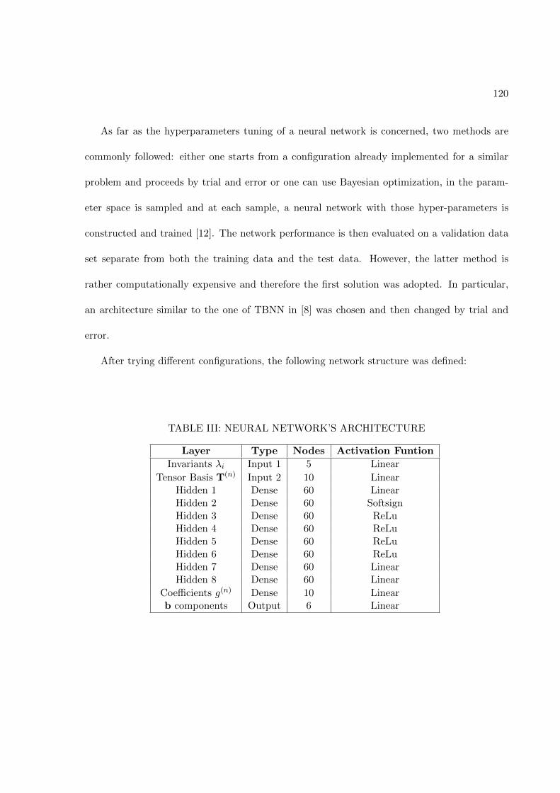
120

As far as the hyperparameters tuning of a neural network is concerned, two methods are

commonly followed: either one starts from a configuration already implemented for a similar

problem and proceeds by trial and error or one can use Bayesian optimization, in the param-

eter space is sampled and at each sample, a neural network with those hyper-parameters is

constructed and trained [12]. The network performance is then evaluated on a validation data

set separate from both the training data and the test data. However, the latter method is

rather computationally expensive and therefore the first solution was adopted. In particular,

an architecture similar to the one of TBNN in [8] was chosen and then changed by trial and

error.

After trying different configurations, the following network structure was defined:

TABLE III: NEURAL NETWORK’S ARCHITECTURE

Layer Type Nodes Activation Funtion

Invariants λi Input 1 5 Linear

Tensor Basis T(n) Input 2 10 LinearHidden 1 Dense 60 LinearHidden 2 Dense 60 SoftsignHidden 3 Dense 60 ReLuHidden 4 Dense 60 ReLuHidden 5 Dense 60 ReLuHidden 6 Dense 60 ReLuHidden 7 Dense 60 LinearHidden 8 Dense 60 Linear

Coefficients g(n) Dense 10 Linearb components Output 6 Linear

121

The activation functions mentioned in Table III are defined by the following expressions:

• Linear activation function ΦL(x) = x

• ReLu activation function ΦR(x) = max(0, x)

• Softsign activation function ΦS(x) =x

1 + |x|

where each function operates element wise on(Wkxk−1 + bk

)of generic layer k.

The distibution of activation functions has been chosen by fixing the same number of hidden

layers of Ling’s TBNN [8]-namely 8 - and through trial and error. The chosen configuration

is the one that allowed to achieve the lowest final RMSE. The general principal driving the

trial and error procedure was that the function g(n)(λi) had to be highly non-linear to be able

to fit a wide variety of different flows. This justify the use of nonlinear activation functions

Softsign and ReLu.The other crucial characteristics of the model are listed and summed up in

the following Table IV, where:

• Shuffling refers to the practice of shuffling validation data after each epoch of the training

phase. This technique avoids the network to learn a pattern linked to the order in which

the data are presented in batches [26].

• Zeros biases initialization means that all layers’ biases are initialized to 0 before training

[26].

• Glorot Uniform is a standard weight initialization; draws samples from a uniform distri-

bution within [-limit, limit] where limit is√

6/(in+ out) where in is the number of input

units in the weight tensor and out is the number of output units in the weight tensor [26].

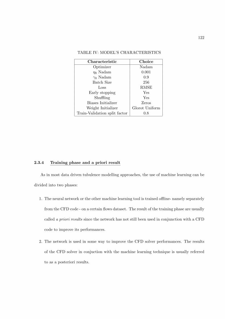
122

TABLE IV: MODEL’S CHARACTERISTICS

Characteristic Choice

Optimizer Nadamη0 Nadam 0.001γ0 Nadam 0.9Batch Size 256

Loss RMSEEarly stopping Yes

Shuffling YesBiases Initializer ZerosWeight Initializer Glorot Uniform

Train-Validation split factor 0.8

2.3.4 Training phase and a priori result

As in most data driven tubulence modelling approaches, the use of machine learning can be

divided into two phases:

1. The neural network or the other machine learning tool is trained offline- namely separately

from the CFD code - on a certain flows dataset. The result of the training phase are usually

called a priori results since the network has not still been used in conjunction with a CFD

code to improve its performances.

2. The network is used in some way to improve the CFD solver performances. The results

of the CFD solver in conjuction with the machine learning technique is usually referred

to as a posteriori results.

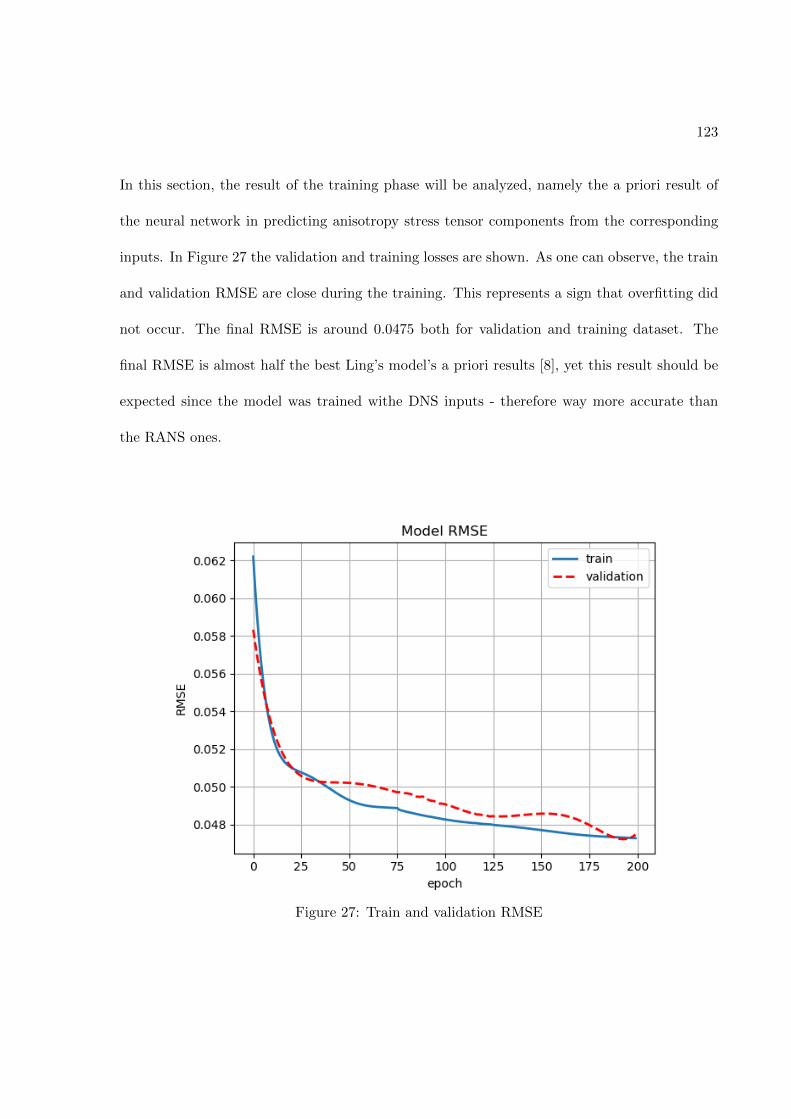
123

In this section, the result of the training phase will be analyzed, namely the a priori result of

the neural network in predicting anisotropy stress tensor components from the corresponding

inputs. In Figure 27 the validation and training losses are shown. As one can observe, the train

and validation RMSE are close during the training. This represents a sign that overfitting did

not occur. The final RMSE is around 0.0475 both for validation and training dataset. The

final RMSE is almost half the best Ling’s model’s a priori results [8], yet this result should be

expected since the model was trained withe DNS inputs - therefore way more accurate than

the RANS ones.

Figure 27: Train and validation RMSE

124

In order to visualize the result, the model was used to predict the anisotropy stress tensor

for one flow of the dataset - the Square Duct Flow. The outcome is showed in Figure 28. Only

the lower left quadrant of the duct is shown, and the streamwise flow direction is out of the

page. The first column show the predictions of the TBNN and the true DNS anisotropy values

are shown in the right column for comparison. In comparsion, the baseline LEVM completely

fails to predict the anisotropy values. It predicts zero anisotropy for b11, b22, and b12. This

is due to the fact that the LEVM does not predict any secondary flows in the duct, so the

mean velocity in the x1 and x2 directions - the one in the transverse plane shown above-is zero,

causing S11, and S22 to be zero [8]. Since the flow is periodic in the x3 direction,S33 is also

zero. As a result, b components are all zeros [8]. On the contrary, the TBNN is not only able

to predict the value of the anisotropy stress tensor components, but also to pick its trends on

the transverse section of the square duct.

125

Figure 28: Prediction of Reynolds stress anisotropy tensor on the Duct Flow case

126

2.3.5 Embedment of the neural network into the CFD solver

A scheme of the approach proposed in this work has already been shown in Figure 3. In

Figure 29, the steps involved in the embedment of the neural network into the CFD solver (b)

are shown in comparison to the standard LEVM approach (a). All the passages have already

been explained in detail above. The steps differing from the standard LEVM model have been

highlighted in red. Basically, insted of directly applying Equation 1.34 to the inputs listed on

top of Figure 29a, deriving from previous computations of the solver at iteration n, a different

set of inputs - top of Figure 29a - are nondimensionalized,normalized and fed to the TBNN.

The output is the anisotropy stress tensor predicted by the network. It is important to stress

again that the use of the neural network as described in Figure 29 differs from the standard

application of machine learning methods in the data driven turbulence modelling approaches.

Indeed, the machine learning method is usually used as a post-processing technique to correct

the RANS anisotropy stress tensor; it receives in input the quantities of interest of the converged

standard RANS model and predicts an anisotropy stress tensor field that is imposed as fixed

in the further iteration of the RANS model.

Here, instead, the machine learning is used to replace the LEVM function correlating b to

velocity gradients and turbulent quantities, and therefore it must be called at each iteration

of the solver. As for this last practical aspect, one problem that had to be faced was that the

model was trained using Python- in particular Keras library - whereas the CFD solver was

coded in Matlab.

127

Figure 29: Embedment of the neural network into the CFD solver

One possibility consisted in computing the network’s inputs in the Matlab solver and pass

to the Python code at each iteration. However, calling the Python script from Matlab and

reloading the Keras model proved extremely time expensive, compared to the solver’s iteration

time. As a solution, the weigths and biases of the model were extracted from the Keras network

and the matrices and vectors were imported in matlab. After that, the same model architecture

was coded in Matlab, since it simply consists of matrices multiplications.

CHAPTER 3

RESULTS

3.1 Application to the turbulent channel flow case

The Tensor Basis Neural Network’ performance was analyzed on the same case on which

the CFD RANS solver was validated- namely the fully developed turbulent channel flow at

Reτ = 544- due to the availability of reference DNS data for comparison [25]. Moreover, the

channel flow was chosen because, in this case, the performance of the LEVM in predicting the

Reynolds stress tensor’s components yields good result only for the shear stress 〈uv〉, as it will

be later shown. This is due to the intrinsic limits of Equation 1.34, in which the anisotropy

stress tensor components are assumed to be in a linear relation with the mean strain rate tensor.

Yet, in the fully developed region of the channel flow, such a tensor is reduced to:

〈S〉 =

0

1

2

∂〈u〉∂y

0

1

2

∂〈u〉∂y

0 0

0 0 0

(3.1)

since 〈v〉 = 0, 〈w〉 = 0 and the variation of the variables occurs only on the direction orthogonal

to the walls y, namely∂

∂x= 0 and

∂

∂z= 0.

128

129

Now, since according to the LEVM:

aLEVM = Cµk2

ε〈S〉 (3.2)

with aLEVM being the anisotropy stress tensor predicted with the LEVM, it is clear that the

only non-zero component of such a tensor will be a12 and that therefore tensor aLEVM will

have the following form:

aLEVM =

0 a12 0

a12 0 0

0 0 0

(3.3)

As a consequence, by recalling (Equation 1.20), the Reynolds stress tensor predicted by the

LEVM will be:

uiuLEVMj =

2

3k a12 0

a122

3k 0

0 02

3k

(3.4)

Hence, when applying a RANS model using the LEVM to the turbulent channel flow case,

all the diagonal components of the Reynolds stress tensor will be predicted with the same value.

In Figure 30 the Reynolds stresses’ profiles obtained with the CFD RANS solver run with the

standard LEVM are shown.

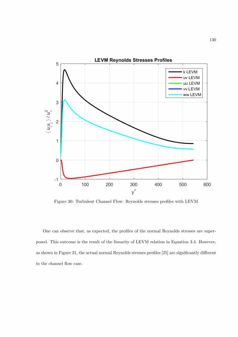
130

Figure 30: Turbulent Channel Flow: Reynolds stresses profiles with LEVM

One can observe that, as expected, the profiles of the normal Reynolds stresses are super-

posed. This outcome is the result of the linearity of LEVM relation in Equation 3.4. However,

as shown in Figure 31, the actual normal Reynolds stresses profiles [25] are significantly different

in the channel flow case.

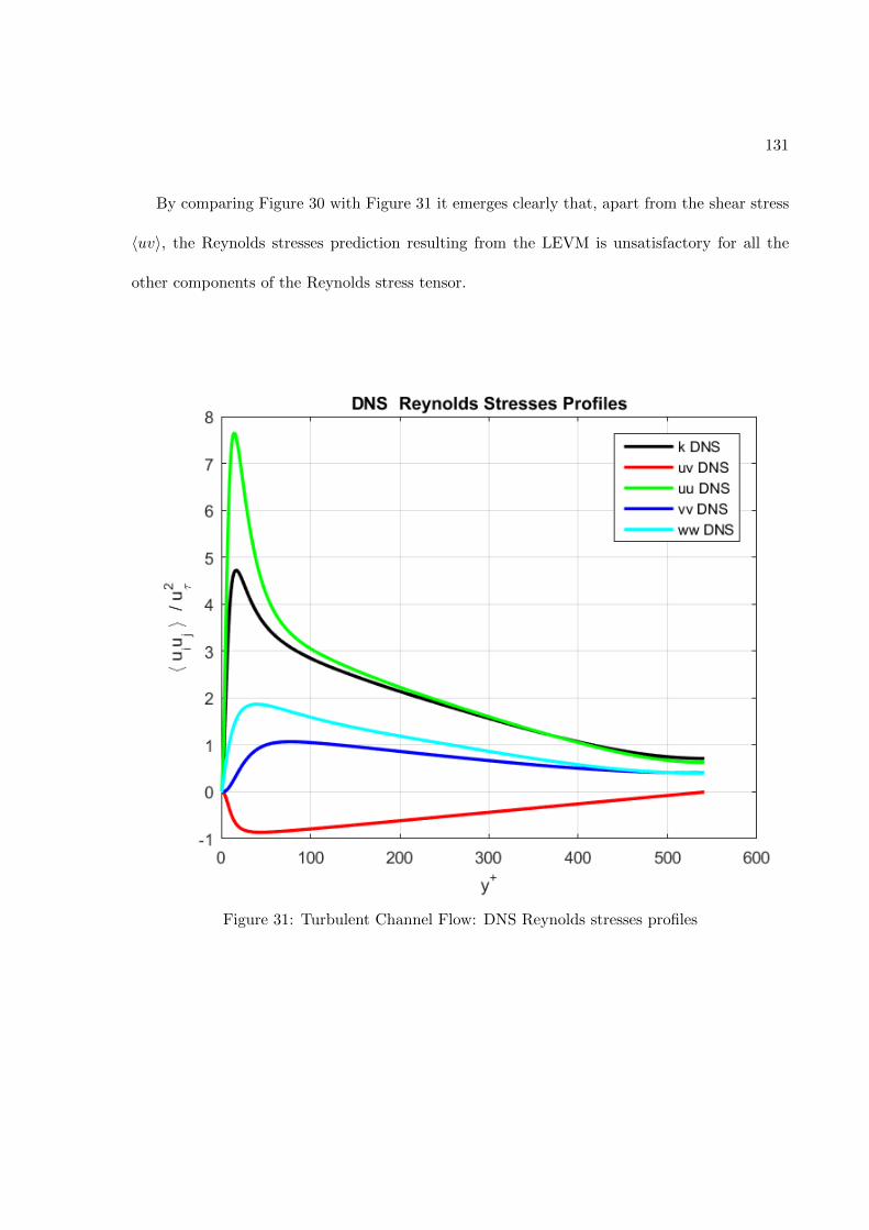
131

By comparing Figure 30 with Figure 31 it emerges clearly that, apart from the shear stress

〈uv〉, the Reynolds stresses prediction resulting from the LEVM is unsatisfactory for all the

other components of the Reynolds stress tensor.

Figure 31: Turbulent Channel Flow: DNS Reynolds stresses profiles

132

Interestingly, an analogue result would be obtained with all fully developed flow cases in

which the variation of the quantities occurs only in one direction - such as for example the

Couette Flow. In most of this cases,however, the normal stress profiles are not the same, and

therefore the prediction of LEVM proves flawed. It is now interesting to compare the predictive

performances of LEVM and TBNN in terms of Reynolds stresses.

In the following figure, the DNS and LEVM Reynolds stresses profiles are compared with

the first prediction of the TBNN, namely on the prediction of the network based on the inputs

of the converged standard RANS.

As one can easily observe in Figure 32, the first prediction of the TBNN significantly out-

performs the LEVM in all zones of the channel height, apart from the shear stress 〈uv〉 for a

certain y+ range. In particular the Reynolds normal stresses’ profiles differ from each other

and are much more accurate than the LEVM ones.

This is due to the fact that the General Eddy Viscosity model of Equation 1.36 involves not

only the mean strain rate tensor 〈S〉 = T(1) but a basis of 10 symmetric and invariant tensors

derived from second and third order products of 〈S〉 and 〈R〉.

This formulation of the Reynolds stresses model incorporates non-linear terms and therefore,

even when the 〈S〉 has only one non-zero component, the contribution of the other tensors allows

to predict distinct profiles for the Reynolds normal stresses.

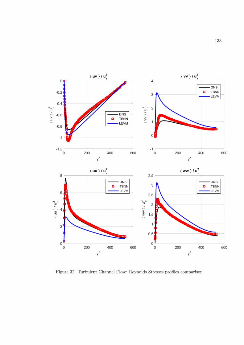
133

Figure 32: Turbulent Channel Flow: Reynolds Stresses profiles comparison

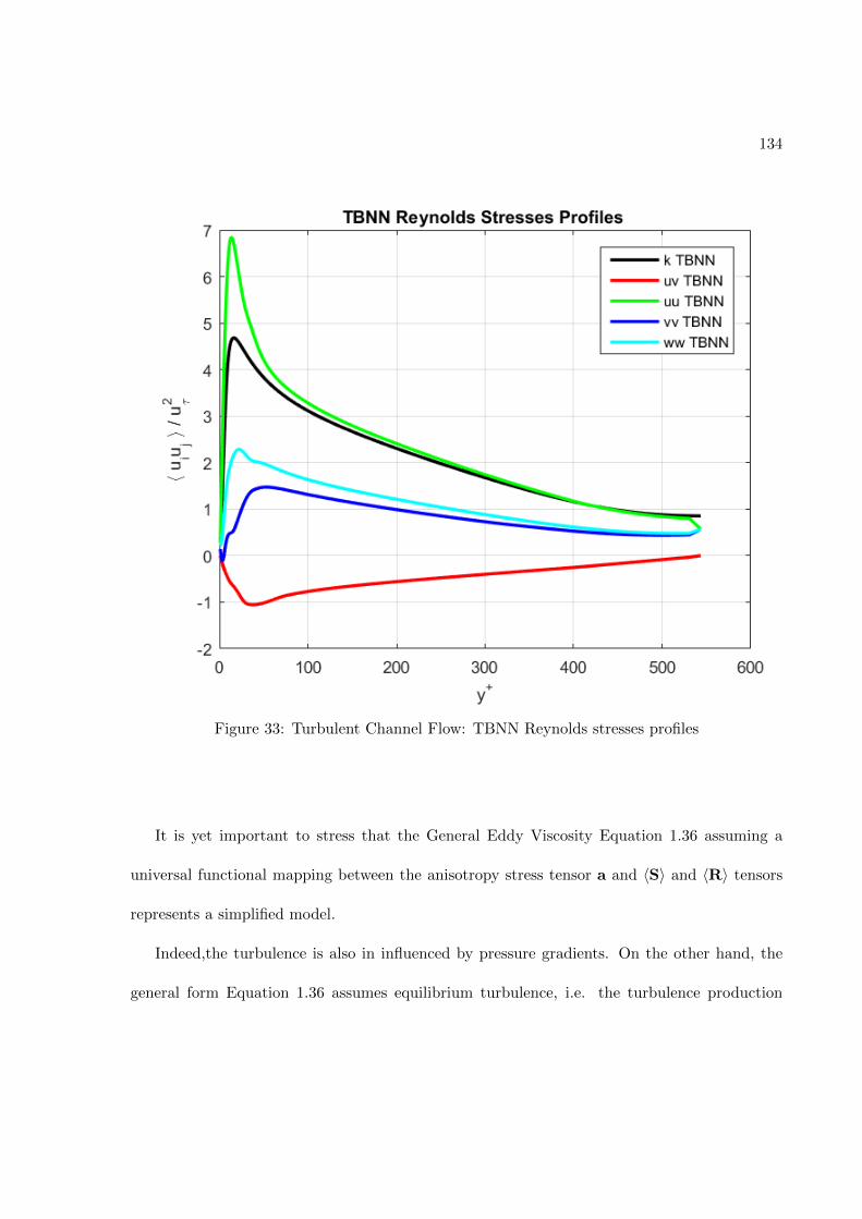
134

Figure 33: Turbulent Channel Flow: TBNN Reynolds stresses profiles

It is yet important to stress that the General Eddy Viscosity Equation 1.36 assuming a

universal functional mapping between the anisotropy stress tensor a and 〈S〉 and 〈R〉 tensors

represents a simplified model.

Indeed,the turbulence is also in influenced by pressure gradients. On the other hand, the

general form Equation 1.36 assumes equilibrium turbulence, i.e. the turbulence production

135

balances dissipation everywhere in the field. With this assumption, the Reynolds stress at

location x only depends on the local gradients of mean velocity at the same location ∇〈U〉(x)

[1].

However, the convection and diffusion of turbulence exist in many real applications, indi-

cating strong non-equilibrium effects and making this single-point-based turbulent constitutive

law invalid [1]. Hence, a certain discrepancy between the TBNN and the DNS data is justified

by the limits of the assumptions leading to Equation 1.36.

It is now interesting to observe how the different tensors T(n) contribute to the final nondi-

mensional anisotropy stress tensor a. It is crucial to recall that, if g(1) = −Cµ = −0.09 and

g(n) = 0 for n > 1, the General Eddy Viscosity model reduces itself to the LEVM. Hence, it

is also interesting to observe the coefficient g(1) predicted by the TBNN and compare it to the

value that results in the LEVM. This is shown inFigure 34. As it can be observed, the coefficient

g(1) predicted by the TBNN has a value close to the LEVM one, yet not on the whole channel

height. Indeed, the two values are particularly close in the log-law region - approximately for

y+ > 30 - where g(1)TBNN holds an almost constant value.

Instead, near the wall and near the channel’s axis, the coefficient deviates significantly from

the value −Cµ. This result is perfectly reasonable: the value of constant Cµ for the LEVM

has been calibrated to match experimental results obtained in the log-law region of turbulent

channel flows, and the LEVM proves correct in this flow region; as a consequence, one can

expect the TBNN to look for a model similar to the LEVM .

136

Figure 34: Coefficient g(1) predicted by TBNN at first solver iteration

On the contrary, LEVM fails in the near-wall region and this is the reason why a low-Re

k − ε model with damping functions was adopted. The damping function fµ of Abe-Kondoh-

Nagano model depends, among other quantities, from the wall distance y+ , which is not an

input in the General Eddy Viscosity model Equation 1.36.

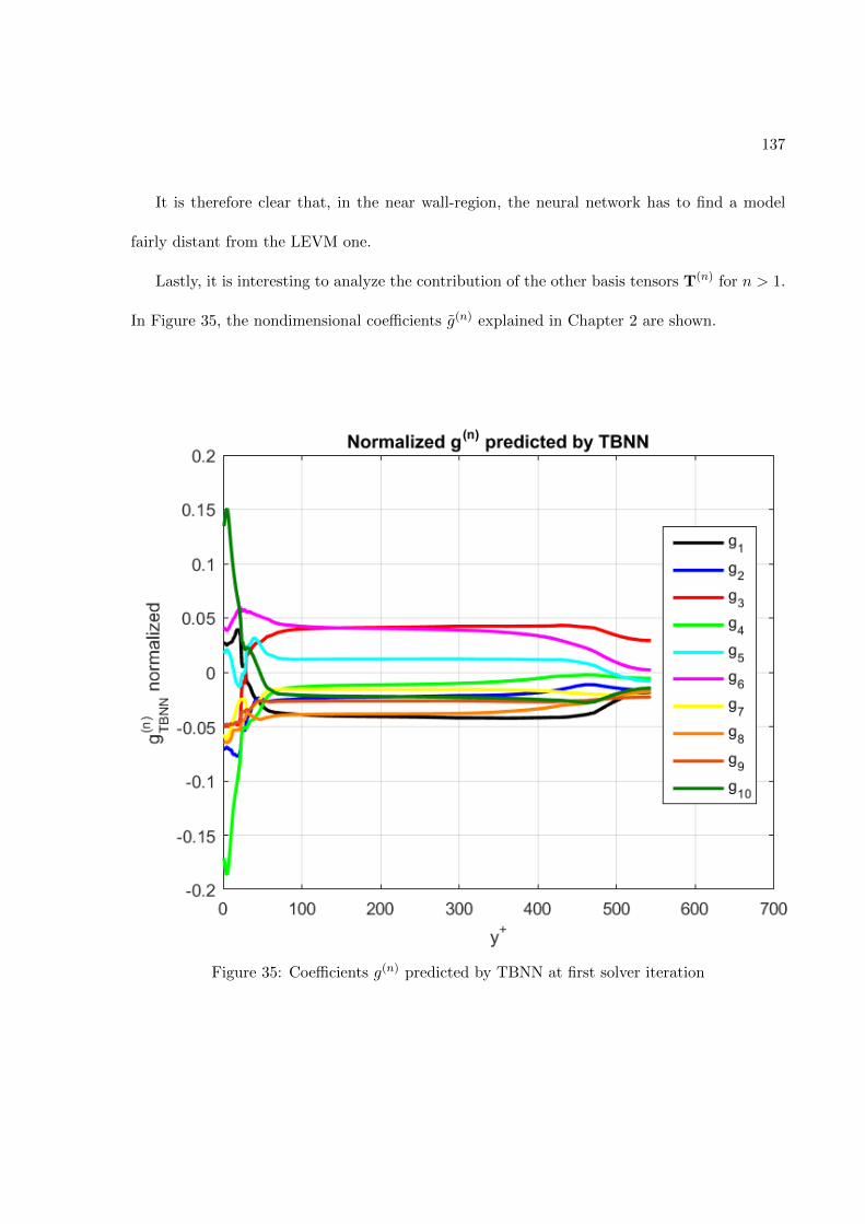
137

It is therefore clear that, in the near wall-region, the neural network has to find a model

fairly distant from the LEVM one.

Lastly, it is interesting to analyze the contribution of the other basis tensors T(n) for n > 1.

In Figure 35, the nondimensional coefficients g̃(n) explained in Chapter 2 are shown.

Figure 35: Coefficients g(n) predicted by TBNN at first solver iteration

138

It is interesting to observe that:

• None of the coefficient is identically null, and therefore all the basis tensors contribute to

b. Since the LEVM is outperformed by the TBNN in the Reynolds stresses prediction, it

is fair to conclude that the linear relation of LEVM is limited and that including higher

order non-linear tensors into the prediction of b can significantly improves the CFD

RANS solver performance. This is true, even though the Reynolds stress anisotropy is

not the only source of uncertainty in the RANS equations, which also rely on approximate

transport equations for k and ε [8].

• All the coefficients hold an approximately constant value in the log-law region, whereas

near the wall their profiles are much more noisy. This may be an indication of the fact

that, in the near wall region, an important variable is the wall distance y+, and that it

should be included in the General Eddy Viscosity model as an additional input. Indeed, for

y+ < 30′ the TBNN has to look for a less smooth function in compensation to accomodate

the prediction to the DNS values.

• Near the channel axis y = δ, all coefficients g(n) → 0. This can be explained by the fact

that: (∂〈u〉∂y

)y=δ

= 0 (3.5)

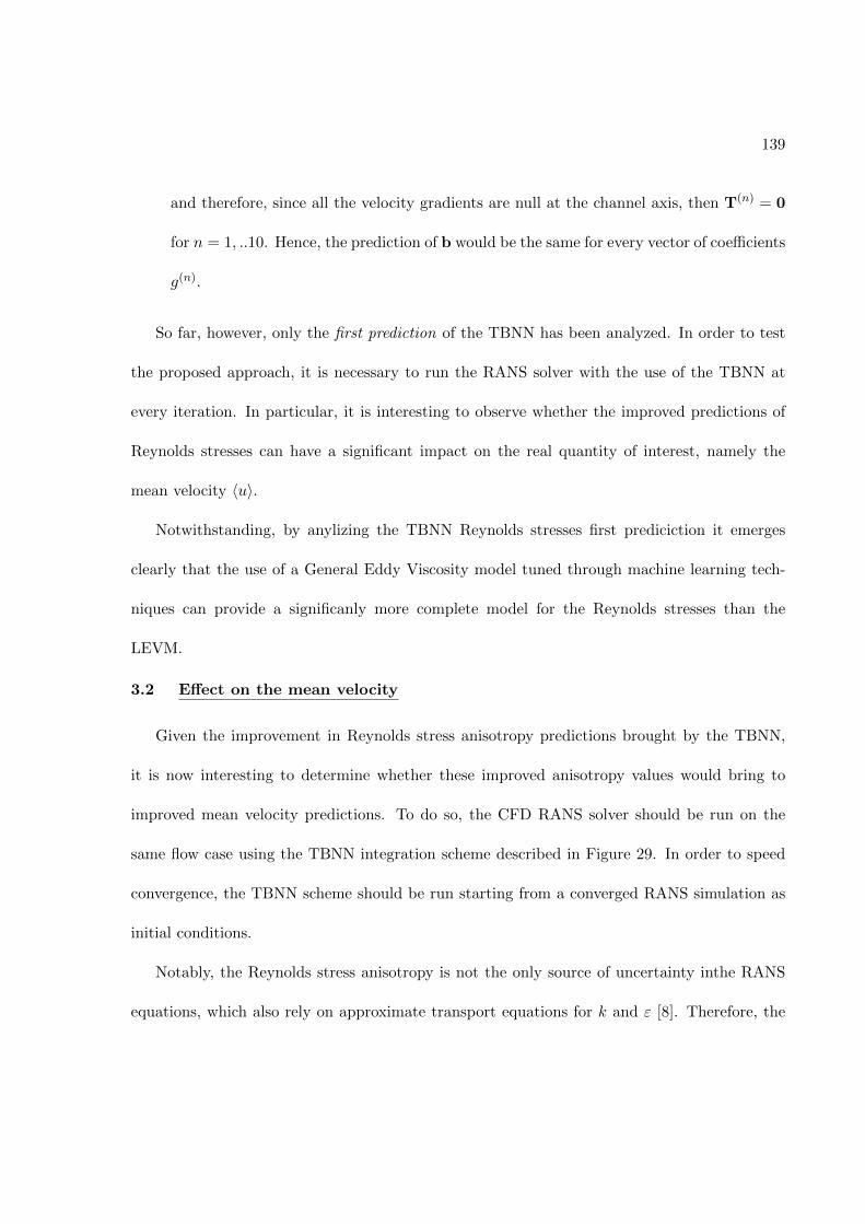
139

and therefore, since all the velocity gradients are null at the channel axis, then T(n) = 0

for n = 1, ..10. Hence, the prediction of b would be the same for every vector of coefficients

g(n).

So far, however, only the first prediction of the TBNN has been analyzed. In order to test

the proposed approach, it is necessary to run the RANS solver with the use of the TBNN at

every iteration. In particular, it is interesting to observe whether the improved predictions of

Reynolds stresses can have a significant impact on the real quantity of interest, namely the

mean velocity 〈u〉.

Notwithstanding, by anylizing the TBNN Reynolds stresses first prediciction it emerges

clearly that the use of a General Eddy Viscosity model tuned through machine learning tech-

niques can provide a significanly more complete model for the Reynolds stresses than the

LEVM.

3.2 Effect on the mean velocity

Given the improvement in Reynolds stress anisotropy predictions brought by the TBNN,

it is now interesting to determine whether these improved anisotropy values would bring to

improved mean velocity predictions. To do so, the CFD RANS solver should be run on the

same flow case using the TBNN integration scheme described in Figure 29. In order to speed

convergence, the TBNN scheme should be run starting from a converged RANS simulation as

initial conditions.

Notably, the Reynolds stress anisotropy is not the only source of uncertainty inthe RANS

equations, which also rely on approximate transport equations for k and ε [8]. Therefore, the

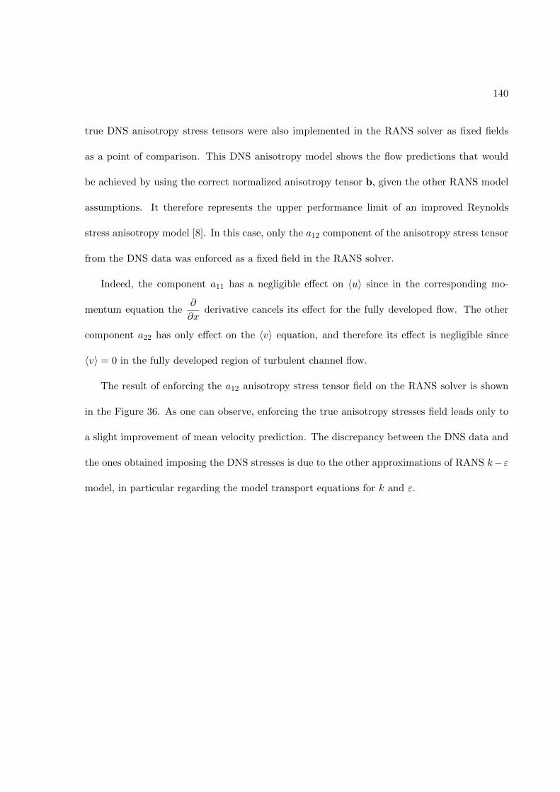
140

true DNS anisotropy stress tensors were also implemented in the RANS solver as fixed fields

as a point of comparison. This DNS anisotropy model shows the flow predictions that would

be achieved by using the correct normalized anisotropy tensor b, given the other RANS model

assumptions. It therefore represents the upper performance limit of an improved Reynolds

stress anisotropy model [8]. In this case, only the a12 component of the anisotropy stress tensor

from the DNS data was enforced as a fixed field in the RANS solver.

Indeed, the component a11 has a negligible effect on 〈u〉 since in the corresponding mo-

mentum equation the∂

∂xderivative cancels its effect for the fully developed flow. The other

component a22 has only effect on the 〈v〉 equation, and therefore its effect is negligible since

〈v〉 = 0 in the fully developed region of turbulent channel flow.

The result of enforcing the a12 anisotropy stress tensor field on the RANS solver is shown

in the Figure 36. As one can observe, enforcing the true anisotropy stresses field leads only to

a slight improvement of mean velocity prediction. The discrepancy between the DNS data and

the ones obtained imposing the DNS stresses is due to the other approximations of RANS k−ε

model, in particular regarding the model transport equations for k and ε.

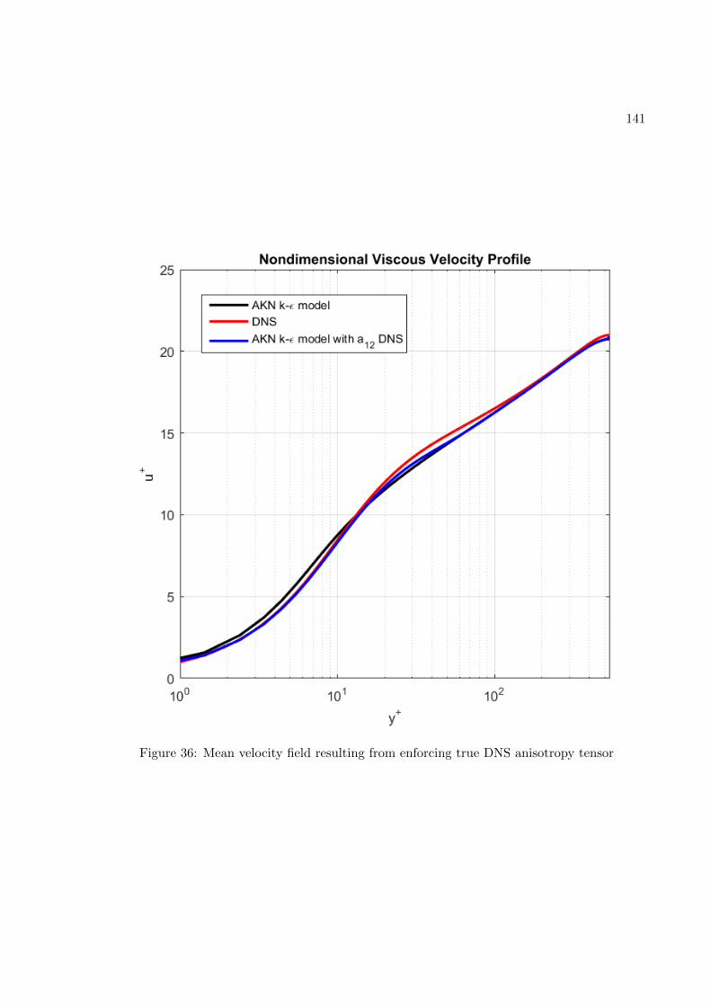
141

Figure 36: Mean velocity field resulting from enforcing true DNS anisotropy tensor

142

Now, by running the CFD RANS solver on the turbulent channel flow case using the TBNN

integration scheme described in Figure 29, it has been obtained:

Figure 37: Mean velocity field resulting from the TBNN approach

143

In Figure 37 above, the predicted mean velocity field 〈u〉 at various iterations n of the

CFD RANS solver running with the TBNN scheme is shown. Iteration n=0 correspond to the

converged RANS solution obtained with the standard LEVM. As one can observe, the mean

velocity profile tend to diverge from the correct DNS one as the iterations increase.

This result is surprisingly negative, if one considers the improvement in the anisotropy

stress tesnsor prediction showed by the TBNN in Figure 32 compared to the LEVM. In order

to interpret the results, a magnification of the 〈uv〉 component in Figure 32 predicteb by TBNN

at first iteration is shown below in a semilogarithmic plot - as the mean velocity one.

This 〈uv〉 component of the Reynolds stress tensor is particularly relevant since, in this

particular flow case, it is the only one affecting the mean velocity field. By observing the

comparison between the LEVM and TBNN profiles, one can obseve that in two regions - y+ < 8

and y+ ∈ [20, 90] - of the channel’s height the TBNN performs worse than the LEVM in the

prediction.

Interestingly enoughh, the TBNN outperforms the LEVM in all the flow regions for all

the other tensor’s components as it results from Fig.(Figure 32). Yet, the normal stresses do

not have any effect on the x momentum equation for 〈u〉. Comparing Fig.(Figure 38) and

Fig.(Figure 37) one can observe that the regions of the flow where the TBNN and the DNS

profiles diverges are the one where the 〈uv〉 prediction of the TBNN is less accurate than the

LEVM one.

As a consequence one can infer that:

144

Figure 38: Turbulent Channel Flow: TBNN 〈uv〉 predicted profile

• The TBNN significantly outperforms the LEVM at iteration 1 in the prediction of normal

stresses but the shear Reynolds stress prediction is worse in the near wall region and in

the first part of the log-law region.

• The only Reynolds stresses component that affects the 〈u〉 field is the shear one and

therefore the 〈u〉 profile predicted with the TBNN is worsened in the regions where the

predictions of 〈uv〉 are worse.

145

• The worsened 〈u〉 profiele brings to a worsened∂〈u〉∂y

profile, which is the main input

to the TBNN. Indeed, by observing the different profiles in Fig.(Figure 37), it emerges

clearly that in the viscous wall region the slope of 〈u〉 curve deviates significantly fromt

the true one.

• The worsened input to the TBNN leads to an even worse prediction of the shear Reynolds

stress and, iteratively, the solver diverges from the correct profile. One should also con-

sider, indeed, that the TBNN can be much more unstable than an analytical function and

therefore it is not granted that the model will have relevant convergence issues.

CHAPTER 4

CONCLUSION

A deep learning approach to RANS turbulence modelling was presented. In an attempt to

improve the standard LEVM for the closure of two-equations RANS models, a neural network

with an architecture analogue to Ling’s work [8] was trained on a large dataset of flows and then

tested on the turbulent channel flow case. The network’s architecture allows to embed Galilean

invariance into the output tensor using a higher-order multiplicative layer. This ensures that

predicted anisotropy tensor lay on a invariant tensor basis. The invariant Tensor Basis Neural

Network was shown by Ling to have significantly more accurate predictions than a generic MLP

that did not have any embedded invariance properties [8].

Yet, differently from the major approaches followed so far in the data driven turbulence

modelling field, the TBNN was not used as a post-processing corrector tool to predict the

Reynolds stresses field b(x) from the inputs of a converged standard RANS solution. Indeed,

the TBNN was trained on DNS data only, in the attempt to find a machine learning mapping

between the anisotropy stress tensor and the inputs of Pope’s General Eddy Viscosity model to

replace the LEVM model at each iteration of the CFD RANS solver. Interestingly, the LEVM

can be seen as the Pope’s GEVM where only one of the 10 coefficients have been tuned. Hence,

in this approach we tested the ability of the network to learn about the underlying flow regimes

present in different flow configurations [8] and to provide a general, more complete model for

146

147

che RANS closure problem.The accuracy of the TBNN was explored in both an a priori and an

a posteriori sense.

In the a priori results, corresponding to the training phase of the network, the TBNN showed

a significant improvement in accuracy compared to [8] in terms of Root Mean Squared Error.

From a visual analysis of the prediction performance for the Square Duct Flow case, it emerged

how the TBNN model is able to predict both the qualitative and quantitative trends of the

Reynolds stresses, significantly outperforming the LEVM.

As for the a posteriori evaluation, the TBNN was used as a replacement of the LEVM

in a self-coded RANS solver using the low-Re Abe-Kondoh-Nagano version of k − ε model.

The approach was tested on a turbulent channel flow case for which DNS data were available

for comparison [25]. We began our analysis by assessing the performance of the TBNN in

predicting various components of the anisotropic Reynolds stress tensor and found that,at first

iteration, the TBNN outperforms the classical LEVM except for the shear component in some

flow regions.

Now, it was of interest to determine wether the improved Reynolds stresses prediction would

translate into better predictions of the mean axial velocity field 〈u〉. Unfortunately, in this flow

case, the only Reynolds stress tensor component affecting the mean velocity field is the shear

one. Hence, in the flow regions where the TBNN Reynolds stresses prediction proved worse

than the LEVM ones, the 〈u〉 profiles deviates from the true DNS one, thus leading to a global

worse result in terms of mean velocity. The convergence properties of the network resulted as

148

well in a serious issue, with the 〈u〉 profile deviating from the DNS one more and more as the

iterations went on.

To sum up, the approach yielded very promising a priori results yet, when tested on the

specific flow case, the globally improved Reynolds stress predictions did not translate into

an improved prediction of the mean flow field. Several avenues for future exploration can

however be devised. First of all, it would be interesting to test the TBNN on a different flow

configuration, maybe a more complex one, in which all the Reynolds stress components affect

the mean velocity fields. Another further aspect to improve would be the convergence properties

arising from the substitution of an analytical function with a TBNN at each iteration of a code.

Lastly, another possible way to explore would be to include more inputs in the Pope’s GEVM

that the network tries to reply, to account for example for pressure gradient and non-locality of

the Reynolds stress tensor. As far as the last solution is concerned, it is important to mention

that, adding tensors and gradients as inputs of the GEVM significantly enlarge the tensor basis

[2], thus making both more complex and computationally expensive to tran the TBNN.

CITED LITERATURE

1. Wu, J.-L., Xiao, H., and Paterson, E., .: Physics-informed machine learning approachfor augmenting turbulence models: A comprehensive framework. Physical ReviewFluids, Jul 2018.

2. Wang, J.-X., Wu, J.-L., and Xiao, H.: A physics informed machine learning approach forreconstructing Reynolds stress modeling discrepancies based on DNS data. PhysicalReview Fluids, Feb 2017.

3. Duraisamy, K.: Status, emerging ideas and future directions of turbulence modeling re-search in aeronautics. Technical Report 219682, NASA scientific and technicalinformation (STI), 2017.

4. Duraisamy, K., Alonso, J., and Durbin, P.: A framework for turbulence modeling using BigData. Technical report, NASA Aeronautics Research Mission Directorate (ARMD),Jan 2015.

5. Ling, J., Templeton, J., and Reese, J.: Machine learning strategies for systems with invari-ance properties. Journal of Computational Physics, 2016.

6. Duraisamy, K., Iaccarino, G., and Xiao, J.: Turbulence modeling in the age of data. AnnualReview of Fluid Mechanics, 51:357–377, 2019.

7. Pope, S. B.: Turbulent Flows. Cambridge, United Kingdom, Cambridge University Press,2000. Reprinted 2017.

8. Ling, J., Kurzawski, A., and Templeton, J.: Reynolds averaged turbulence modellingusing deep neural networks with embedded invariance. Journal of Fluid Mechanics,807:155–166, 2016.

9. Ferziger, J. and Peric, M.: Computational methods for fluid dynamics. Springer, 2002.

10. ANSYS Support Davoudabadi, P.: The most accurate and advanced turbulence capabilities.https://support.ansys.com/staticassets/ANSYS/Conference/Confidence/

Chicago/Downloads/most-accurate-advanced-turbulence-capabilities.pdf.[Online; accessed 05/01/2019].

149

150

CITED LITERATURE (continued)

11. Pope, S.: A more general effective-viscosity hypothesis. Journal of Fluid Mechanics,72(2):331–340, 1975.

12. Fang, R., Sondak, D., Protopapas, P., and Succi, S.: Deep learning for turbulent chan-nel flow. https://arxiv.org/abs/1812.02241, Dec 2018. [Online; accessed04/15/2019].

13. Wikipedia contributors: Finite volume method — Wikipedia, the free encyclope-dia. https://en.wikipedia.org/w/index.php?title=Finite_volume_method&

oldid=929950836, 2019. [Online; accessed 06/05/2019].

14. Leap Australia: Tips & tricks: Estimating the first cell height for correct y+. https:

//www.computationalfluiddynamics.com.au/. [Online; accessed 05/15/2019].

15. ANSYS Theory Guide: Enhanced wall treatment. https://www.afs.enea.it/project/

neptunius/docs/fluent/html/th/node101.htm. [Online; accessed 05/15/2019].

16. Sondak, D., Pletcher, R., and Vandalsem, W.: Wall functions for the k − ε turbulencemodel in generalized nonorthogonal curvilinear coordinates. https://doi.org/

10.31274/rtd-180813-11746. [Online; accessed 04/06/2019].

17. Abe, K., Kondoh, K., and Nagano, Y.: A new turbulence model for predicting fluidflow and heat transfer in separating and reattaching flows-i. Flow field calculations.International Journal of Heat and Mass Transfer, 37(1):138–151, 1994.

18. Suga, K.: Recent developments in eddy viscosity modelling of turbulence. Technical report,R & D Review of Toyota CRDL, 1998.

19. Gorji, A., Seddighi, M., A., C., Vardy, A., O’Donoghue, T., Pokrajac, D., and He, S.: Acomparative study of turbulence models in a transient channel flow. Computer &Fluids, 89:111–123, 2014.

20. Jagadeesh, P. and Murali, K.: Application of low-Re turbulence models for flow simula-tions past underwater vehicle hull forms. Journal of Naval Architecture and MarineEngineering, Jan 2005.

21. Harlow, F. and Welch, J.: Numerical calculation of time-dependent viscous incompressibleflow of fluid with free surface. Physics of Fluids, 8(12):2182–2189, 1965.

151

CITED LITERATURE (continued)

22. Liu, F. and Zheng, X.: A strongly coupled time-marching method for solving theNavier–Stokes and k − ω turbulence model equations with multigrid. Journal ofComputational Physics, 128:289–300, 1996.

23. Patankars, S.: Numerical Heat Transfer and Fluid Flow. Taylor & Francis, 1980.

24. NPTEL:: Solution of Navier-Stokes equations for incompressible flows using SIMPLE andMAC algorithms. https://nptel.ac.in/courses/112104030/pdf/lecture27.

pdf. [Online; accessed 04/03/2019].

25. Lee, M. and Moser, R.: Direct numerical simulation of turbulent channel flow up to Reτ= 5200. Journal of Fluid Mechanics, 774:395–415, 2015.

26. Keras Documentation: Keras, the Python deep learning library. https://keras.io/.[Online; accessed 02/15/2019].

27. Huser, A.: Direct Numerical Simulation of a Flow in a Square Duct. PhD thesis, Universityof Colorado at Boulder, 1992.

28. Wu, Z., Laurence, D., and Afgan, I.: Direct simulation of hot jet in cold channel cross-flow with temperature mixing. https://doi.org/10.17632/7nx4prgjzz.4, 2018.[Online; accessed 03/13/2019].

29. Laval, J.-P.: Direct Numerical Simulations of converging-diverging channel flow. https:

//turbmodels.larc.nasa.gov/Other_DNS_Data/conv-div-channel12600.html,2011. [Online; accessed 03/14/2019].

30. Temmerman, L., Bentaleb, Y., and Leschziner, M.: Large Eddy Simulation of theflow over periodic hills. https://turbmodels.larc.nasa.gov/Other_LES_Data/

2dhill_periodic.html, 2005. [Online; accessed 03/14/2019].

31. Lardeau, S.: Large-eddy simulation of turbulent boundary layer separation from a roundedstep. https://turbmodels.larc.nasa.gov/Other_LES_Data/curvedstep.html,2012. [Online; accessed 03/14/2019].

32. Schlatter, P. and Orlu., R.: Assessment of direct numerical simulation data of turbulentboundary layers. Journal of Fluid Mechanics, 842:128–145, 2018.

33. Lee, M. and Moser, R.: Extreme-scale motions in turbulent plane Couette flows. Journalof Fluid Mechanics, 659:116–126, Sept 2010.

152

CITED LITERATURE (continued)

34. Jaitley, U.: Why data normalization is necessary for machine learning models. https:

//medium.com/@urvashilluniya/. [Online; accessed 02/15/2019].

35. Almaliki, Z.: Standardization vs normalization. https://medium.com/@zaidalissa/.[Online; accessed 02/15/2019].

36. Ruder, S.: An overview of gradient descent optimization algorithms. https://ruder.io/

optimizing-gradient-descent/. [Online; accessed 02/15/2019].

37. Bushaev, V.: Adam,latest trends in deep learning optimization. https://

towardsdatascience.com/. [Online; accessed 02/15/2019].

38. Brownlee, J.: Gentle introduction to the Adam optimization algorithm for deep learning.https://machinelearningmastery.com/. [Online; accessed 02/15/2019].

39. Tracey, B., Duraisamy, K., and Alonso, J.: A machine learning strategy to assist turbulencemodel development. Technical report, AIAA SciTech Forum, Jan 2015.

40. Kuzmin, D. and Mierka, O.: On the implementation of the k − ε turbulence model inincompressible flow solvers based on a finite element discretization. InternationalJournal of Computing Science and Mathematics, Jan 2019.

41. Rechia1, A., Naji, H., M. G., and Marjani, A.: Numerical simulation of turbulent flowthrough a straight square duct using a near wall linear k−εmodel. The InternationalJournal of Multiphysics, 1(3), 2007.

42. Versteeg.H.G. and Malalasekera, W.: An Introduction to Computational Fluid Dynamics.The Finite Volume Method. Pearson, 2nd edition, 2007.

43. Lamberti, L.: Data Driven Modelling of Turbulent Flows using Artificial Neural Networks.Master’s thesis, Polytechnic University of Turin, July 2019.

VITA

NAME Luca Lamberti

EDUCATION

Master of Science in “Mechanical Engineering, University of Illinois atChicago, Jan 2020, USA

Master Degree in “ Mechanical Engineering ”, Jul 2019, Polytechnic ofTurin, Italy

Bachelor’s Degree in Mechanical Engineering, Jul 2017, Polytechnic ofTurin, Italy

LANGUAGE SKILLS

Italian Native speaker

English Full working proficiency

2017 - IELTS examination (8/9)

2014 - Certificae in Advanced English ESOL (CAE)

SCHOLARSHIPS

Fall 2018 Italian scholarship for final project (thesis) at UIC

Fall 2018 Italian scholarship for TOP-UIC students

2017 Einaudi campus scholarship

2014 -2016 Camplus scholarship

2014-2017 ’Young Talents’ program member at Polytechnic University of Turin

TECHNICAL SKILLS

Average level C/C++ programming; CAD/FEM modelling with NX Siemens; 1DModelling with LMS Amesim; Python programming & use of Tensor-flow library

Advanced level CAD modeling with CATIA, Solidworks; Use of SU2 CFD Software;Matlab programming

153

154

VITA (continued)

WORK EXPERIENCE AND PROJECTS

Nov - Dic 2019 Graduate Engineer at Toyota Motor Europe

Jan - May 2019 Research Assistantship (RA) position (10 hours/week) with full tuitionwaiver plus monthly wage at University of Illinois at Chicago

2018 - 2019 Strategy Division member for Student Team H2Polito at PolythecnicUniversity of Turin

2017 - 2018 CAD designer and Strucutural Analyst for Student Team PACE atPolythecnic University of Turin

July 2017 European Innovation Academy participant