Cross-Country Diﬀerences in the Optimal Allocation of ...

Cross-Country Differences in the Optimal Allocation of Talent and Technology⇤

Tommaso Porzio

†

University of California, San Diego

February 20, 2017

Abstract

I model an economy inhabited by heterogeneous individuals that form teams and choose an

appropriate production technology. The model characterizes how the technological environment

shapes the equilibrium assignment of individuals into teams. I apply the theoretical insights to

study cross-country differences in the allocation of talent and technology. Their low endowment

of technology, coupled with the possibility of importing advanced technology from the frontier,

leads poor countries to a different economic structure – one with a stronger concentration of

talent and a larger cross-sectional productivity dispersion. As a result, the efficient equilibrium

in poor countries resembles economic features that are often cited as evidence of misallocation.

Micro data from countries of all income levels document cross-country differences in the allocation

of talent that support the theoretical predictions. A quantitative version of the model suggests

that a sizable fraction of the larger productivity dispersion documented in poor countries is due

to differences in the efficient allocation.

⇤This paper is based on my PhD dissertation at Yale University. This project deeply benefited from numerousconversations with colleagues and advisors. First of all, I am extremely grateful to my advisors, Mikhail Golosov,Giuseppe Moscarini, Nancy Qian, Aleh Tsyvinski, and Chris Udry, for their invaluable guidance and support andto Benjamin Moll, Michael Peters and Larry Samuelson for helpful suggestions and stimulating discussions. I alsothank for very helpful comments Joseph Altonji, Costas Arkolakis, David Atkin, Lorenzo Caliendo, Douglas Gollin,Pinelopi Goldberg, Samuel Kortum, David Lagakos, Ilse Lindenlaub, Costas Meghir, Marti Mestieri, Nicholas Ryan,Alessandra Voena, Nicolas Werquin, and Noriko Amano, Gabriele Foà, Sebastian Heise, Ana Reynoso, GabriellaSantangelo, Jeff Weaver, and Yu Jung Whang. Last, but not least, I received many insightful comments from seminarparticipants at BU, Bocconi, Columbia, CMU (Tepper), Georgetown, IIES, Wisconsin-Madison, McGill, Princeton,Stanford, Toronto, UCSD, Yale, and the NBER Fall Development Meeting.

†9500 Gilman Drive, La Jolla, CA 92093, email: [email protected].

1 Introduction

Low-income countries have low labor productivity and, thus, produce lower output for thesame amount of input. At the same time, cross-sectional productivity dispersion is larger inlow-income countries: while most individuals see their labor produce very little output, someothers enjoy fairly high productivity.1 Often, this excessive productivity dispersion is interpretedas evidence of market frictions that prevent reallocation of inputs to more-productive firms andsectors or adoption of the best available technologies.2

In this paper, I explore an alternative view. I argue that the larger productivity dispersionmay be a natural side effect of poor countries having access to advanced technologies importedfrom the distant technology frontier. The economic mechanism I propose entails two insights.

First, low-income countries have the unique opportunity to adopt technologies, discoveredelsewhere, that are much more advanced than their current level of development. As long asindividuals differ in their returns from adoption – due to heterogeneous ability, for example – onlysome would take advantage of this opportunity. Thus, heterogeneous adoption leads naturally tothe dispersion of used technology and, as a result, of productivity. Take India, for example. Ithas approximately the level of GDP per capita that the United States had at the beginning of the20

th century. Nonetheless, we would not be surprised to spot a person on the street in Kolkatausing a cell phone to shop online with Flipkart, the Indian alternative to Amazon. And yet, stillin Kolkata, another person could be cruising through the city on a pulled rickshaw, which was acommon mode of transportation already in the 19

th century. A wide range of technologies coexistin India today - arguably, many more than in the United States at the beginning of the 20

th

century, when cell phones and the internet were still decades away from being invented.Second, I show that the opportunity to adopt advanced technology determines the way in

which individuals of heterogeneous ability form production teams – that is, the allocation of tal-ent – in low-income countries and that, at the same time, the different allocation of talent affectsthe dispersion of used technology itself. In fact, high-skilled individuals have higher returns fromusing advanced technology, and so they cluster together in the few economic niches where moderntechnology is pervasive. But, in equilibrium, if all high-skilled individuals form teams with eachother, the rest of the economy is left with only low-skilled individuals who have low inherent pro-ductivity and few incentives to improve their technology. The concentration of similarly talentedindividuals within the same teams is, thus, both a consequence and a catalyst of productivity andtechnology dispersion.

The interaction of these two insights shapes the economic structure of poor countries. Someeconomic niches attract most of the high-skilled individuals and adopt the advanced technology.The rest of the economy is left without talent and, thus, finds it convenient to rely on backward,and cheaper, technology. Summing up, the possibility of adopting technology from the frontierendogenously generates cross-sectional dispersion and dual economies in poor countries.

1See Caselli (2005), and Hsieh and Klenow (2009) (Figure I of TFPQ, not the more famous Figure II of TFPR).2Notable exceptions are Lagakos (2016), Lagakos and Waugh (2013), Caunedo and Keller (2016), and Young

(2013).

1

The described economic forces are not mere theoretical possibilities. In this paper, I use microdata from several countries to show that talent is more concentrated in less-developed ones, astheory predicts. Moreover, I show, through the lens of a quantitative version of the model, thatthese differences are sizable and that the outlined mechanism can contribute to explaining thelarger productivity dispersion in poor countries.

Overview. The paper is organized in four sections.In Section 2, I develop a theoretical framework to analyze the joint determination of the

allocation of talent and technology. The economy is inhabited by a continuum of individuals ofheterogeneous ability. Production requires three inputs: a manager, a worker, and a technology.The production function satisfies two assumptions. First, output is more sensitive to manager’sability than to the worker’s. Second, there is complementarity between technology and the abilityof both the manager and the worker. Each individual chooses his occupation: whether to be aworker or a manager. Managers choose the ability of the worker to hire and the level of technologyto operate. More-advanced technologies are costlier but allow higher labor productivity. Thecompetitive equilibrium of this setting decentralizes the Pareto efficient allocation; I characterizeit. The endogenous sets of managers and workers are the main objects of interest. Given these twosets, complementarity dictates positive assortative matching – more-able managers are matchedwith more-able workers – and so the unique equilibrium is pinned down. As is standard, eachindividual chooses the occupation in which he has a comparative advantage. The main difficultyof this setting is that the comparative advantages are endogenous and depend on the technologychoice of each team. If all the teams pick the same technology, the higher skill sensitivity of outputdictates that the most skilled individuals would have a comparative advantage in being managers.Endogenous technology choice introduces a new trade-off: in equilibrium, each individual usesa higher technology if he decides to be a worker. Hence, to use a more advanced technology– that increases the marginal value of one’s skills, – one needs to choose an occupation thatis less skill-intensive. This trade-off is modulated by the technological environment. The maintheoretical result is that the more important is the choice of an appropriate technology – i.e.,the larger is the elasticity of the optimal technology choice to ability, relative to the production’sasymmetry in skill sensitivity – the smaller is the ability gap between two individuals workingtogether. This result shows that the allocations of talent and technology (and, thus, productivity)are tied together: when technology is dispersed, there is a lower ability gap between managersand workers.

In Section 3, I explicitly model cross-country differences in the cost of technology. WhenI use the term “technology,” I refer to the input of the production function, which is simplya productivity term that multiplies labor input.3 This notion of technology depends on twoelements: (i) the choice of which vintage of technology to use – e.g., to rely on animal or electricpower; and (ii) the amount of capital of the used vintage – e.g., how many bullocks are purchased.More modern vintages have a lower variable cost of technology, but a larger fixed one to be

3I use technology to distinguish it from productivity, which is output divided by the number of workers, and,thus, takes into account worker ability.

2

operated. Countries differ in their local technology vintage, and in each country, every productionteam can use the local vintage without paying any fixed cost. However, to import more modernvintages from other countries, teams must pay a fixed cost that increases in the distance betweenthe chosen vintage and the local one. The described environment yields a country-specific costof technology. Moreover, the elasticity of the optimal technology to the ability of team membersdepends on the distance of a country from the technology frontier, defined as the gap between thelocal vintage and the most advanced one available. This result is generated by the heterogeneityof returns to technology adoption: even in countries far from the frontier, the most able teams paythe fixed cost to import modern vintages, while the less able ones prefer to rely on local vintages.

Combining the insights from Sections 2 and 3, the theory provides sharp predictions on cross-country differences in economic structure. First, the model predicts that the efficient competitiveequilibrium generates larger technology and labor productivity dispersion in poor countries. Largeproductivity dispersion is often associated with misallocation. In this framework, instead, it isgenerated through differences in endowments: poor countries are endowed with less-advancedlocal technology vintages and this leads, in equilibrium, to larger productivity dispersion. Second,the theory predicts cross-country differences in the way in which people form production teams.Specifically, talent should be more concentrated in countries far from the frontier: an empiricalprediction, to the best of my knowledge, unique to this model.

In Section 4, I confront the model’s predictions on the allocation of talent with the data. Inthe main empirical exercise, I use large-sample labor force surveys for 63 countries to show thatin the countries farther from the technology frontier – i.e., with lower relative GDP per capita –the concentration of talent is higher. In the data, neither teams nor individual skills are directlyobserved. I show that under two assumptions – (i) education is correlated with ability; and(ii) individuals within the same industry use a more similar technology than those in differentindustries – we can construct, using the distribution of schooling within and across industries,an empirical measure of concentration of talent that aligns with the one defined in the model. Iconstruct this measure for each country-year pair and show how it varies as a function of distanceto the frontier, both in the cross-section and in the time-series. I first compare countries in thecross-section. The concentration of talent is negatively correlated with GDP per capita, andthe magnitude of cross-country differences is sizable. I then compare middle-income countriestoday (such as Mexico and Brazil) with the United States in 1940, which was at the same levelof development – but, critically, was closer to the technology frontier. Middle-income countriestoday have a higher concentration of talent than the U.S. did in the past. This result alleviates theconcern that cross-sectional differences are merely capturing differences in levels of development.Finally, I compare the growth paths of South Korea and the United States in the past sevendecades. In the United States, the concentration of talent has remained relatively unchanged,consistent with the fact that is has grown steadily as a world leader (i.e., on the frontier). Incontrast, South Korea has seen a rapid decline in the concentration of talent as it has approachedthe technology frontier.

I then provide further supporting evidence from occupation data: managers are, on average,

3

less skilled in poor countries, while workers are more skilled, as the theory predicts. However, thedefinitions of managers and workers in the data are not perfectly comparable across countries.For this reason, I also focus on two specific occupations: retail cashiers and motor vehicle drivers.Both of these occupations require simple tasks (they would correspond to workers in the model)but use advanced technologies – i.e., the cash register and the combustion engine. The modelpredicts that in poor countries, retail cashiers and motor vehicle drivers should be relatively moreskilled. This prediction is confirmed in the data.

I end Section 4 by using use the World Bank Enterprise Surveys to indirectly validate themain model assumptions – the tasks and skill-technology complementarities – and to confirm thatthe allocation of talent is different in poor countries even at the firm level.

Finally, In Section 5, I write a computational version of the model and show that the cross-country differences in the concentration of talent are consistent with sizable differences in within-country productivity dispersion. Specifically, I define a notion of agriculture in the model, andI estimate the model to target cross-country differences in the concentration of talent and theagricultural productivity gap in rich countries. I then predict agricultural productivity gaps inpoor countries and show that the model, once disciplined with the cross-country differences in theallocation of talent, accounts for approximately one third of the larger agricultural productivitygap in poor countries.

Related Literature. The theoretical contribution of the paper is to combine two strands ofthe literature and show that they interact non-trivially. I consider an environment in whichindividuals form production teams – following the seminal work of Lucas (1978), Kremer (1993)and, more recently, Garicano and Rossi-Hansberg (2006) – and, at the same time, choose anappropriate production technology – along the lines of the work of Atkinson and Stiglitz (1969),Basu and Weil (1998), and Acemoglu and Zilibotti (2001). I show that allowing teams to choosea production input, technology, that is complementary to the team members’ ability changes theequilibrium assignment. To the best of my knowledge, this is a new insight for the literatureon team formation. At the same time, taking endogenous team formation into consideration isrelevant to understanding the distribution of technology within a country. Specifically, equilibriumteam formation links the right and left tails of the technology distribution: the possibility ofadopting advanced technology generates a right tail of high-technology teams that gather all thetalent, thus crowding out high-skilled individuals from the rest of the economy; and creating a lefttail of low technology and, thus, low productivity, teams. In other words, modern technology insome economic niches within a country comes at the cost of backward technology elsewhere. Tothe best of my knowledge, this is a new insight for the literature on appropriate technology andtechnology adoption. In studying the distribution of technology and productivity as the resultof agents’ maximization behavior, my work is similar to Perla and Tonetti (2014). In allowingcountries to import more-advanced technologies from abroad, my work is similar to Buera andOberfield (2016). Neither of these papers considers the endogenous allocation of talent.

A growing literature studies the allocation of talent in Roy models of occupational choice, inwhich individuals draw a vector of occupation-specific abilities that determine their comparative

4

advantage; – one recent application is Hsieh et al. (2016). My work, instead, considers hetero-geneity along one single trait, a general skill. Most of the literature with occupational choice andunidimensional skills, starting from the seminal Lucas (1978), makes assumptions on the produc-tion function such that the highest skilled have a comparative advantage in being managers. Inmy setting, instead, the comparative advantages and, thus, the pattern of matching, is endoge-neous. Specifically, it depends on the equilibrium distribution of technology. In this respect, mywork mostly resembles Kremer and Maskin (1996). While Kremer and Maskin (1996) studies howchanges in skill distributions can impact the pattern of matching, I keep the skill distributionconstant and show, instead, that endogenous choice of technology shapes the pattern of matching.I also provide a new solution method and develop a quantitative version of the model.

Similarly to Kremer (1993), this paper uses a frictionless model to understand cross-countrydifferences in organization of production. However, Kremer (1993) focuses on average differencesacross countries – e.g., in poor countries, firms are, on average, smaller – while I focus on cross-country differences in the within-country distribution of economic activity – e.g., in poor countries,large and small firms coexist, while in rich ones, all firms are similar in size.

The idea that distance to the frontier may impact the organization of production is presentin Acemoglu et al. (2006), which studies selection into entrepreneurship with credit constraints.I see my work as complementary to theirs. Roys and Seshadri (2014) also studies differencesacross countries in the way in which production is organized. It uses a quantitative version ofGaricano and Rossi-Hansberg (2006) in which human capital is endogenously accumulated, asin Ben-Porath (1967). Cross-country differences are generated by changes in the distribution oftalent, and not by changes in the pattern of matching, which, in their work, is fixed ex-ante.

The application of the theory to developing countries fits into the debate on dual economies.Through the lens of the model, the fact that individuals in poor countries have the ability to adoptadvanced technology from the frontier leads to the endogenous formation of dual economies. Thisview is original but resembles most closely that of La Porta and Shleifer (2014), which emphasizeshow duality is tightly linked to economic development.

Finally, two other papers, Acemoglu (1999) and Caselli (1999), argue that the technologicalenvironment and the allocation of workers to jobs are connected. Acemoglu (1999) focuses onthe interaction between labor market frictions and the fact that firms have to commit ex-antewhether to create jobs for high- or low-skilled workers, and, it shows the conditions for a separatingequilibrium to exist. Caselli (1999) shows that when new technologies are adopted, the most skilledindividuals are the ones most likely to start using them, thus separating themselves from the restof the economy. Neither of these papers considers complementarity between individuals workingtogether. My work focuses exactly on this latter channel and characterizes how the properties ofthe technological environment change the overall production complementarity, thus changing theassignment of workers to jobs.

5

2 A Model of Technology Choice and Allocation of Talent

I develop an assignment model in which heterogeneous individuals form production teams andchoose an appropriate and costly technology.

2.1 EnvironmentThe economy is inhabited by a continuum of mass one of individuals, indexed by their ability

x ⇠ U [0, 1]. Individuals with higher x are more able. Each individual supplies inelastically oneunit of labor and has a non-satiated and increasing utility for the unique final good produced inthe economy.

Production. Production of labor input requires two individuals to form a team: a managerand a worker. A manager of ability x

0 paired with a worker of ability x produces f (x

0, x) units

of labor inputs, where f (x

0, x) is strictly increasing in both arguments and twice continuously

differentiable.4 Production of the final good requires the labor input to be combined with aproduction technology a 2 R, that multiplies labor input. There is a continuum of availabletechnologies in the economy, and technology a has a cost c (a), in units of output. This cost isincreasing, convex, and twice continuously differentiable. A production team (a, x

0, x) where a

is the technology, x

0 is the ability of the manager, and x is the ability of the worker producesg (a, x

0, x) units of the final output

g

�

a, x

0, x

�

= af

�

x

0, x

�

� c (a) .

Assumptions on Production of Labor Input. I assume that the production function oflabor input satisfies the following three5 properties:

1. f

1

(x, x) > f

2

(x, x), for all x 2 [0, 1];

2. f

12

(x

0, x) > 0, for all (x0, x) 2 [0, 1]⇥ [0, 1];

3. f

1

(x, y) > f

2

(z, x), for all (x, y, z) 2 [0, 1]⇥ [0, 1]⇥ [0, 1].

(1) captures the fact that, for a given technology and partner, the individual’s skills are more useful(has a greater effect on output) if he is employed in a managerial position. This assumption iscommon in the literature. See, for example, the seminal paper by Lucas (1978), which assumesthat only the manager’s ability matters for production, and Garicano and Rossi-Hansberg (2006),which builds from primitives a production function that features this property. (2) capturescomplementarity in production between tasks. This is a natural assumption, pervasive in theliterature. (3) is a Spence-Mirrlees condition that separates types into occupations by imposingthat, if all teams use the same technology, the complementarity between types is sufficiently weakrelative to the skill asymmetry, and, thus, high-skilled individuals have a comparative advantage in

4Note the slight abuse of notation: I refer to x as the ability of an individual in general; however, when I wantto distinguish explicitly between the ability of the manager and that of the worker, I refer to the former as x

0 andto the latter as x.

5Assumption (3) is stronger than (1), which is, formally, a redundant assumption. Nonetheless, it is conceptuallyconvenient to separate the two.

6

the managerial occupation. As I will show, (3) is not sufficient to separate types if the technologychoice is endogenous.

Complementarity Skill-Technology. Assumption (3) implies that

4. g

12

(a, x, y) > g

13

(a, z, x) � 0 for all (a, x, y, z) 2 R⇥ [0, 1]⇥ [0, 1]⇥ [0, 1] .

Technology and skills are complementary, consistent with most of the evidence for both devel-oped and developing countries (see Goldin and Katz (1998), Foster and Rosenzweig (1996) andSuri (2011)). Further, the manager’s ability is more relevant than the worker’s for generating highreturns from technology, as emphasized in recent studies that highlight the role of managers intechnology adoption (see Bloom and van Reenen (2007) and Gennaioli et al. (2013)).

The functional form assumption of g implicitly assumes a specific strength of the complemen-tarity between skills and technology. This restriction is useful for tractability but is not necessaryfor the main results. In Appendix C, I consider a more general specification for g.6

Assignment of Talent to Teams. Production requires one manager and one worker. Indi-viduals’ ability x is observable, and individuals are not restricted ex-ante to belong to eithergroup. As a result, an allocation in this setting comprehends an occupational choice function,! (x) : [0, 1] ! [0, 1], which defines the probability that an individual x is a worker, and a match-ing function, m (x) : [0, 1] ! [0, 1], which assigns to each individual x the type of the manager hewould be matched with if he decides to be a worker.7

2.2 Competitive EquilibriumThe competitive equilibrium of this economy is given by five functions: optimal technology

↵ (x

0, x) : [0, 1]⇥ [0, 1] ! R; profit ⇡ (x) : [0, 1] ! R; wage w (x) : [0, 1] ! R; occupational choice

! (x) : [0, 1] ! [0, 1]; and matching m (x) : [0, 1] ! [0, 1] such that

1. each team chooses the optimal technology

↵

�

x

0, x

�

= argmax

a2Raf

�

x

0, x

�

� c (a) ;

2. each manager chooses the type of worker to hire, taking into account the optimal technologythat the pair would choose and taking as given the equilibrium wage schedule

⇡ (x) = max

z2[0,1]↵ (x, z) f (x, z)� w (z)� c (↵ (x, z)) ;

3. the matching function is consistent with manager’s optimality

m (z

⇤(x)) = x

6The Appendix is available online at https://sites.google.com/a/yale.edu/tommaso-porzio/.7The definition of m (x) as a function rather than a correspondence might seem restrictive. However, it is not.

In fact, I prove in a previous version of this paper, (Porzio (2016)), that for the currently considered case in whichx ⇠ U [0, 1], m (x) is indeed a function and not a correspondence. This is a standard result in the literature, andfor this reason I omit the details here.

7

where z

⇤(x) is the solution to the manager’s problem;

4. each individual chooses the occupation that pays him the higher income or randomizesamong them if ⇡ (x) = w (x): ! (x) satisfies

! (x) 2 arg max

z2[0,1](1� z)⇡ (x) + zw (x) ;

5. the sum of wage and profit of a team equals its produced output, for all x

⇡ (m (x)) + w (x) = g (↵ (m (x) , x) ,m (x) , x) .

This restriction also guarantees that the goods market clears; and

6. labor market clears for each individual type x, and all individuals are employed. That is,for each type, the mass of less-skilled workers must equal the mass of managers matchedwith these workers according to m, and the mass of managers and workers must sum to

xˆ

0

! (z) dz =

xˆ

0

(1� ! (m (z))) dz

1ˆ

0

! (z) dz +

1ˆ

0

(1� ! (z)) dz = 1.

Proposition 1: Existence and Pareto Efficiency.A competitive equilibrium exists and is Pareto Efficient.Proof. See appendix. �

Equilibrium uniqueness is not guaranteed in this environment. Nonetheless, this is not aconcern since the properties of the equilibrium that I characterize in the next section hold for anyequilibrium.

2.3 Equilibrium CharacterizationI now characterize the equilibrium and show how the assignment of talent to teams and the

choice of technology are related.2.3.1 Choice of Technology

A team of a manager of ability x

0 and a worker of ability x picks the technology that maximizesnet output; that is,

↵

�

x

0, x

�

= c

0�1

�

f

�

x

0, x

��

.

The complementarity between technology and labor input and the assumptions on the functionalform of f give the following result.

8

Lemma 1: Appropriate TechnologyThe appropriate technology of a team increases in the skills of both the manager and the worker,but more so in the skills of the manager: ↵

1

> ↵

2

� 0.Proof. See appendix. �

The manager and the worker agree on the choice of technology since it does not affect howthey share output.2.3.2 Manager Problem

Consider a manager of ability x. He picks the optimal type of workers to maximize his profit⇡ (x); that is,

⇡ (x) = max

z2[0,1]↵ (x, z) f (x, z)� w (z)� c (↵ (x, z)) .

The solution of this maximization problem yields the matching function, which assigns to eachworker his manager and satisfies m (z

⇤(x)) = x. The skill complementarity between managers

and workers (f12

> 0) implies that the matching function is increasing.

Lemma 2: Matching Function

The matching function m is increasing: for all (x0, x) 2 [0, 1]

2, if x

0> x and

´x

0

x

! (z) dz > 0,then m (x

0) > m (x).

Proof. See appendix. �

The envelope and first-order conditions give the slopes of the profit and wage functions

⇡

0(x) = ↵

�

x,m

�1

(x)

�

f

1

�

x,m

�1

(x)

�

(1)

w

0(x) = ↵ (m (x) , x) f

2

(m (x) , x) ,

where m

�1

(x) is the inverse of the matching function and, thus, assigns each manager his type ofworker. By definition, m�1

(x) = z

⇤(x), and the function m is invertible due to the fact that it is

strictly increasing over the relevant domain. The slopes of the profit and wage functions determinethe marginal values of skills in each occupation, which, as I will show, drive the occupationalchoice. These values depend on the technology used, the occupation-specific skill sensitivity,and the production partner. In general, an individual has different partners and, thus, differentappropriate technologies whether he is a worker or a manager. The higher the technology used,the more skills are valued – due to skill-technology complementarity. At the same time, themanager’s tasks are different from the worker’s; thus, each occupation is going to have a specificskill sensitivity that affects its overall marginal value of skills.2.3.3 Occupational Choice

I first discuss the optimal assignment to occupations within a team. Two individuals thatwork together use, by assumption, identical technology. As a result, the relative marginal value ofskills in either occupation depends only on the asymmetry in skill sensitivity. Due to the Spence-Mirrlees assumption, the managerial task uses skills more efficiently, and, thus, the more skilledindividual of the team must be the manager.

9

Lemma 3: Occupational Choice within a TeamThe manager of the team is more skilled than the worker of the team: m (x) � x for all x 2 [0, 1].Proof. See below, after Lemma 4. �

The Technology-Occupation Tradeoff. Lemma 3 implies that an individual x is matchedwith a more-skilled partner and, thus, uses a more advanced technology if he decides to be aworker rather than a manager. There is a technology-occupation trade-off: an individual woulduse a higher technology, which gives his skills, ceteris paribus, a higher marginal value, if he selectsinto the less-skill-intensive occupation. As a result, an individual x sees his skills having a highermarginal value as a manager – i.e., ⇡0

(x) � w

0(x) – if and only if the gap in skill sensitivity across

occupations is larger than gap in technology used:

f

1

�

x,m

�1

(x)

�

f

2

(m (x) , x)

| {z }

Skill Sensitivity Gap

� ↵ (m (x) , x)

↵ (x,m

�1

(x))

| {z }

.

Technology Gap

Individuals, as usual, select into the occupation in which they have their comparative advantage.High-skilled individuals have a comparative advantage in the occupation that has the highestmarginal value of skills. Most of the literature8 focuses on functional form assumptions such thatmanagement is more skill-intensive – that is, ⇡0

(x) � w

0(x) 8x. For example, Lucas (1978) uses

a production function that gives w

0(x) = 0: the high-skilled have a comparative advantage in

being managers; thus, the shape of the occupational choice function is known ex-ante and is givenby a cutoff policy that separates types into two connected sets of managers and workers. In mysetting, instead, the comparative advantage of each individual x is endogenous since it depends onthe optimal technology choice of each team. For example, some high-skilled individuals may findtheir skills more rewarded by being workers with a high technology rather than managers with alower one. To solve this complex fixed point, I develop a method to use the necessary conditionsfor optimality, together with market clearing, to characterize the overall equilibrium assignmentand to show how it depends on the shape of f and ↵.

Necessary Conditions. The occupational choice function ! (x) maximizes individual income:

! (x) 2 arg max

z2[0,1](1� z)⇡ (x) + zw (x) . (2)

! (x) divides the type space into subsets in which individuals are managers, workers, or randomizebetween the two occupations. Since the type space is a compact set, (i) individuals that areat the boundaries between two subsets in which two different occupations are chosen, must beindifferent between being a manager or a worker; and (ii) individuals that randomize between thetwo occupations must also be indifferent. For these two groups of individuals, the maximizationproblem (2) provides useful necessary conditions that link the occupational choice to the marginal

8The one notable exception that I am aware of is Kremer and Maskin (1996).

10

values of skills in either occupation.

Lemma 4: Necessary Conditions of Occupational Choice FunctionThe occupational choice function satisfies:

1. for all x such that lim✏!0

! (x� ✏) 2 (0, 1) and lim

✏!0

! (x+ ✏) 2 (0, 1): ⇡

0(x) = w

0(x);


! (x� ✏) = 0 and lim

✏!0

! (x+ ✏) > 0: ⇡

0(x) w

0(x);


! (x� ✏) = 1 and lim

✏!0

! (x+ ✏) < 1: ⇡

0(x) � w

0(x).


Formally, these conditions are derived from the fact that the wage and profit functions mustcross in proximity of an ability type x that is indifferent between either occupation.

I use these necessary conditions to characterize the equilibrium. The proofs of the results areleft to the online appendix. Nonetheless, in order to illustrate the general method I use, I showhere how the necessary conditions can be used to prove Lemma 3.

Proof of Lemma 3. Let x > x

0, ! (x) > 0 and suppose that m (x) = x

0. Then, let x bethe lowest type larger than x

0 with ! (x) > 0. Since ! (x) > 0 and – by market clearing –! (x

0) < 1, then x 2 [x

0, x]. By the necessary conditions, w0

(x) � ⇡

0(x). Substituting in Equation

(1), w

0(x) � ⇡

0(x) becomes ↵(m(x),x)

↵(x,m

�1(x))

� f1(x,m�1

(x)

)

f2(m(x),x)

. Lemma 1 shows that m and m

�1 areincreasing. As a result, x x implies that m (x) m (x) = x

0 x, and, also, x � x

0 impliesthat m

�1

(x) � m

�1

(x

0) = x � x. Therefore, ↵(m(x),x)

↵(x,m

�1(x))

1 since ↵ is increasing in both of his

arguments. The Spence-Mirrlees assumption (3) guarantees that f1(x,m�1

(x)

)

f2(m(x),x)

> 1. This leads toa contradiction and, thus, to m (x) � x. �2.3.4 Technology Choice and Equilibrium Assignment of Talent to Teams

The main characterization result ties the properties of the optimal technology choice ↵ andthe production function f to the assignment of talent to teams.

Proposition 2: Assignment of Talent Across TeamsIn a competitive equilibrium, for any worker x 2 [0, 1] the ability gap between him and his manager,m (x)� x, is bounded above by ⌥ (x) and below by ⇤ (x), where ⌥ (x) and ⇤ (x) depend on f and↵ as follows:

1. Consider two functions f and ˜

f , if for all (x0, y, z) 2 [0, 1]

3 such that x0 � y � z

f1(y,z)

f2(x0,y)

�˜

f1(y,z)

˜

f2(x0,y)

, then ⌥ (x) � ˜

⌥ (x) and ⇤ (x) � ˜

⇤ (x); and

2. consider two functions ↵ and ↵, if for all (x0, y, z) 2 [0, 1]

3 such that x

0 � y � z

↵(x

0,y)

↵(y,z)

�↵(x

0,y)

↵(y,z)

, then ⌥ (x) ˜

⌥ (x) and ⇤ (x) ˜

⇤ (x) 8x 2 [0, 1].


In the appendix, I include the implicit functions that define each bound. The propositionshows that ⇤ (x) m (x) � x ⌥ (x) and that these upper and lower bounds depend on the

11

shape of f and ↵. f and ↵ modulate the technology-occupation trade-off and, thus, change theequilibrium assignment of talent to teams. When there is stronger asymmetry in skill sensitivity,so that high-skilled individuals have a stronger comparative advantage in being managers, thenthe gap between workers and managers widens, since more of the high-skilled find it optimal tobe managers. When, instead, the elasticity of optimal technology choice to the team members’ability increases – i.e., when teams formed by individuals of different ability choose very differentoptimal technologies – the choice of occupation becomes a less important, and the technologyused becomes a more important, determinant of the marginal value of an individual’s skills. Asa result, some high-skilled individuals find it optimal to be workers and, in equilibrium, the skillgaps between workers and their managers decrease.

It is simple to see that when m (x)� x is smaller, talent is more concentrated, as some teamsbring together the high-skilled, and, thus, in equilibrium, other teams are left with low-skilledmanagers and workers. Formally, I define the concentration of talent as follows.

Definition 1: Concentration of TalentConsider two matching functions m and m. Talent is more concentrated according to m if´[m (x)� x]! (x) dx <

´[m (x)� x]! (x) dx. I define 1�

´[m (x)� x]! (x) dx the concentration

of talent.

Proposition 2 shows that the concentration of talent is tightly linked to the strength of eitherside of the technology-occupation trade-off. I next consider two polar cases with respect to thistrade-off and show the conditions under which they emerge.

Definition 2: Segmentation by OccupationTalent is segmented by occupation if x0 > x and ! (x) < 1 imply that ! (x

0) = 0.

Definition 3: Segregation by TechnologyTalent is segregated by technology if x

0> x implies that ↵

�

x

0,m

�1

(x

0)

�

� ↵ (m (x) , x) withprobability one.

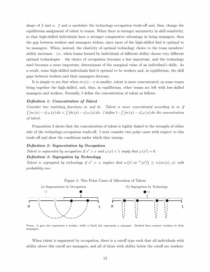
Figure 1: Two Polar Cases of Allocation of Talent(a) Segmentation by Occupation (b) Segregation by Technology

Notes: A grey dot represents a worker, while a black dot represents a manager. Dashed lines connect workers to theirmanagers.

When talent is segmented by occupation, there is a cutoff type such that all individuals withability above this cutoff are managers, and all of those with ability below the cutoff are workers.

12

This case is illustrated in Figure 1a below. When talent is segregated by technology, more-skilled individuals use a higher technology than lower-skilled individuals use. When the function↵ (x

0, x) strictly increases in both its arguments, this requires that m (x) ! x. This second case

is illustrated in Figure 1b.Corollary 1: Conditions for Segregation and Segmentation

If ↵ and f satisfy ↵(x

0,y)

↵(y,z)

<

f1(y,z)

f2(x0,y)

for all (x

0, y, z) 2 [0, 1]

3, with x

0> y > z , then talent is

segmented by occupation and m (x) =

1

2

+ x. If ↵ satisfies ↵(x

0,y)

↵(y,z)

! 1 for all (x0, y, z) 2 [0, 1]

3,with x

0> y > z, then talent is segregated by technology and m (x) ! x.


Figure 2: Lower and Upper Bounds of Ability Gap between Managers and Workers

0 0.5 1 1.5 2 2.5 3

η

0

0.05

0.1

0.15

0.2

0.25

0.3

0.35

0.4

0.45

0.5

Gap b

/w W

ork

ers

and M

anagers

Upper Bound, λ Low

Lower Bound, λ Low

Upper Bound, λ High

Lower Bound, λ High

Numerical Solution, λ Low

Numerical Solution, λ High

Notes: The figure shows the bounds according to Proposition 2 compared with actual values from the numerical solution.

Proposition 2 bounds the concentration of talent, while Corollary 1 shows two limit cases ofit. It is natural to wonder how wide the bounds provided are. The answer depends on the specificchoice of the functional form. To explore whether the bounds can be informative, I provide anexample with simple functional forms. Let f (x

0, x) = x

0(1 + �x), with � 1, and c (a) =

a

1+⌘

1+⌘

,

with ⌘ � 0, which implies that ↵ (x

0, x) = (x

0(1 + �x))

1⌘ . This system of functional forms has two

parameters: lower � generates stronger skill asymmetry, and lower ⌘ generates larger technologygaps. In Figure 2, I plot the upper and lower bounds for the median individual x =

1

2

as a functionof ⌘ and for two different values of �. These bounds are informative. In the same figure, I alsoplot the actual gaps m

�

1

2

�

� 1

2

, computed numerically using the Hungarian algorithm.This section has characterized how the optimal technology choice and the allocation of talent

are linked. The results are characterized in terms of one intuitive property of ↵, the technologygap, rather than in terms of the primitive c (a). In the next section, I model c (a).

13

3 Cross-Country Differences in the Allocation of Talent

I describe a technological environment that yields a country-specific functional form for the costof technology. I characterize the properties of the cost function and obtain sharp predictions forthe relationship between the distance of a country from the technology frontier and its allocationof talent.

3.1 Distance to the Technology Frontier and Cost of TechnologyRecall that the gross output of a team (x

0, x) that uses technology a is af (x

0, x). Technology

a is a multiplicative productivity term.9 More specifically, I think of a as a reduced-form termthat captures two separate elements that determine the team’s productivity: (i) the technologyvintage that a team uses; and (ii) the capital intensity at which the specific technology vintageis operated. Consider an example. In order to grind one hundred pounds of grain into flour inan hour, a team could use either many horse-powered mills or fewer but faster electric mills. Theteam can achieve the same level of “technology” a – one hundred pounds of grain per hour – witheither many units of an old vintage of technology (horse-powered mills) or fewer units of a newervintage of technology (electric mills). Thus, the cost of achieving technology a needs to take intoconsideration (i) the optimal choice of technology vintage and its fixed cost; and (ii) the amountof capital of that technology vintage that is necessary to achieve a and its variable cost.

I describe, consistent with this interpretation of technology a, the world technological envi-ronment.

The Technological Environment. The most advanced vintage of available technology is ¯

t,which represents the technology frontier at a given point in time. Each country is indexed by itslevel of development t ¯

t. All individuals in country t know how to use technology vintage t;hence, they do not need to pay any fixed cost to use it. I will refer to t as the local technologyvintage. The distance of a country from the technology frontier is given by ¯

t � t – that is, thedistance at a given point in time between that country’s level of development and world knowledge.Individuals in each country can decide to import and learn how to use better vintages of technology,up to the frontier one ¯

t, paying a fixed cost. The lower the country’s level of development, thehigher the fixed cost. A more modern technology vintage allows a team to achieve the same levelof productivity a at a lower variable cost, but it has a higher associated fixed cost. Thus, there isa trade-off that leads to the optimal choice of technology vintage.

I summarize this technological environment using a system of equations, from which I thenderive a country-specific cost of technology. The choice of functional forms is guided by parsimonyand tractability, rather than by generality.

Cost of Technology. The cost of achieving productivity level a in country t using the localtechnology vintage is

c

L

(a; t) = �

�⌘t

�⌘

1

(a� a

t

)

1+⌘

1 + ⌘

,

9I call it technology to distinguish it from labor productivity, that is simply defined as output divided by labor.

14

where � captures the productivity improvements across technology vintages; ⌘ captures the within-vintage cost elasticity of technology; and a

t

= ⌫�

t with ⌫ 2 [0, 1] is a non-homotheticity term thatbecomes useful in the limit case described below, but in general can be assumed to be 0. Sinceindividuals already know how to use the local vintage, there is no associated fixed cost. Hence,we should think of c

L

(a; t) as the variable cost component linked to the chosen capital intensity.

1

is a constant term that scales the cost of technology. I choose

1

⌘ ⌘"�1

⌘"

to guarantee thatthe marginal type that decides not to use the local technology does not depend on either t or ¯

t.While restrictive, this provides tractability.

Figure 3: Cost of Technology

Notes: dashed lines represent the cost of technology for one specific technology vintage. The lightest gray line is the costfor the local vintage, while the darkest gray line is the cost for the frontier vintage. The black solid line is the cost oftechnology that takes into account the choice of technology vintage. a

I,t

is the level of technology below which the localvintage minimizes the cost. a

t,t

is the level of technology above which the frontier vintage minimizes the cost.

The cost of achieving productivity level a in country t using an imported technology vintage˜

t is given by

c

I

�

a,

˜

t; t

�

= �

�⌘

˜

t

(a� a

t

)

1+⌘

1 + ⌘

+

�(⌘"�1)

2

�

t

�

"⌘

(

˜

t�t

)

" (1 + ⌘)

,

where

�(⌘"�1)

2

�

t

�

"⌘

(

t�t

)

"(1+⌘)

is the fixed cost associated with learning technology vintage ˜

t; " captures

the elasticity of the cost of technology across vintages;

2

⌘ �

0

� ⌘+1⌘

1⌘"�1 is defined so that the

marginal team that decides to import technology rather than using the local vintage is given by

15

�

0

. I assume that �

0

< f

�

1

2

, 0

�

, so that not all teams decide to import, even when talent issegmented. The fixed cost is increasing in the gap between the current level of development andthe vintage of technology ˜

t to capture that individuals in less-developed countries may have aharder time learning and using more-advanced technologies, and extracting proper returns fromit; coherently with the view that frontier technologies are targeted to the level of development ofrich countries, as in Acemoglu and Zilibotti (2001).

Finally, the cost of achieving productivity level a in country t, taking into consideration theoptimal vintage choice, is given by

c (a; t,

¯

t) = min

⇢

c

L

(a; t) ,min

˜

t¯

t

c

I

�

a,

˜

t; t

�

�

.

I assume that ⌘" < 1 in order for the technology vintage choice to have, possibly, an interiorsolution – i.e., some teams may choose nor the local, nor the frontier vintage.

Optimal Technology. This system of functional forms provides simple solutions for the optimaltechnology ↵.

The cost function c (a; t,

¯

t) is the lower envelope of the costs of technology for each vintage.More-modern vintages have a lower variable cost of productivity, but a higher fixed cost. As aresult, as Figure (3) shows, teams that choose a higher technology minimize costs by choosing amore advanced vintage. The next three Lemmas summarize the cost of technology, the resultingoptimal technology choice, and its properties.Lemma 5: Cost of TechnologyThe cost of a technology c (a; t,

¯

t) is given by

c (a; t,

¯

t) =

8

>

>

>

<

>

>

>

:

�

�⌘t

�⌘

1

(a�a

t

)

1+⌘

1+⌘

if a a

I,t

�

�⌘

"

t

�⌘

"

2

(a�a

t

)

1+⌘

"

1+⌘

"

if a 2�

a

I,t

, a

¯

t,t

�

�

�⌘

¯

t

(a�a

t

)

1+⌘

1+⌘

+

�(⌘"�1)

2

�

t

�

"⌘(t�t)

"(1+⌘)

if a � a

¯

t,t

,

where ⌘

"

⌘ ⌘"�1

"+1

< ⌘, aI,t

= a

t

+ �

t

1

�

1⌘

0

and a

¯

t,t

= a

t

+ �

t

�

⇣1+"

1+⌘

⌘⌘(

¯

t�t)

�

1⌘

0

.Proof. See appendix. �

Lemma 6: Optimal Technology ChoiceThe optimal technology choice of a team (x

0, x) is given by

↵

�

x

0, x; t,

¯

t

�

=

8

>

>

>

<

>

>

>

:

a

t

+ �

t

1

f (x

0, x)

1⌘ if f (x

0, x) �

0

a

t

+ �

t

2

f (x

0, x)

1⌘

" if f (x

0, x) 2 (�

0

,�

1

(t,

¯

t))

a

t

+ �

¯

t

f (x

0, x)

1⌘ if f (x

0, x) � �

1

(t,

¯

t) ,

where �

1

(t,

¯

t) = �

0

�

⌘(⌘"�1)⌘+1 (

¯

t�t). Also, teams with f (x

0, x) �

0

use the local vintage, and teamswith f (x

0, x) � �

1

(t,

¯

t) use the frontier vintage.

16


Lemma 7: Properties of Optimal TechnologyThe optimal technology choice of a team (x

0, x) satisfies:

1. each team would use a higher technology in a country closer to the frontier: for all (x0, x, )↵ (x

0, x; t

0,

¯

t) � ↵ (x

0, x; t,

¯

t) if and only if t0 � t;

2. for a given level of development, the more advanced is the frontier, the higher the technologyused: for all (x0, x) ↵ (x

0, x; t,

¯

t

0) � ↵ (x

0, x; t,

¯

t) if and only if ¯t0 � ¯

t;

3. the technology gap between teams in a country depends only on the distance from the frontier:↵(x,y;t,

¯

t)

↵(y,z;t,

¯

t)

=

↵(x,y;

¯

t�t)

↵(y,z;

¯

t�t)

, where ↵ (x

0, x;

¯

t� t) = ↵ (x

0, x; t,

¯

t) �

�t; and

4. the cutoff �

1

(t,

¯

t) increases in the distance from the frontier.

Proof. See appendix. �A few comments on Lemma 7 are in order. Properties 1 and 2 show that in more-developed

countries, individuals use more-advanced technologies, but at the same time, the presence of mod-ern technology vintages at the frontier also benefits less-developed countries. The third propertyshows that it is not the absolute level of development that matters for the technology gap, but,rather, the distance from the technology frontier. The fourth property says that, everything elseequal, the number of individuals using a modern vintage is increasing in the level of developmentof a country. Nonetheless, some teams in less-developed countries also use the most advancedvintage available. This property of the cost function is consistent with the fact that most moderntechnologies are used even in the poorest regions of the world, with the main difference acrosscountries being that, in rich ones, many more individuals use them; as documented in Comin andMestieri (2016). Cell phones and computers are two salient examples.

Last, and critical, Proposition 3 below shows that in countries far from the frontier, thetechnology gaps across teams are higher. The possibility of countries far from the frontier tochoose whether to import more-advanced technology vintages from abroad leads naturally tolarger gaps in the optimal technology across teams. This result emerges because not everyonefinds it optimal to choose the same technology vintage. At the frontier, however, all individualsuse the same vintage, the frontier one, since there is nothing better available. Putting this resulttogether with the characterization of Section 2, and especially Proposition 2, implies that theconcentration of talent is stronger in countries far from the frontier.

Proposition 3: Technology Gap and Distance to the FrontierThe technology gap increases in the distance from the technology frontier: for all (x0, y, z) 2 [0, 1]

3

such that x0 � y � z, ↵(x

0,y;t,

¯

t)

↵(y,z;t,

¯

t)

� ↵

0(x

0,y;t

0,

¯

t

0)

↵(y,z;t

0,

¯

t

0)

if and only if ¯t� t � ¯

t

0 � t

0.Proof. See appendix. �

17

Corollary 2: Assignment of Talent and Distance to the FrontierBoth the upper and lower bounds of the ability gap between a worker and his manager are decreasingin the distance to the technology frontier.Proof. See appendix. �

The distance of a country from the frontier is not directly observable in the data. Lemma 8shows that we can use the GDP per capita of a country to proxy for the distance to the frontier.

Lemma 8: GDP per capita and Distance to the FrontierThe GDP per capita of a country is given by

Y (t,

¯

t) =

1ˆ

0

g (↵ (m (x) , x; t,

¯

t) ,m (x) , x)! (x) dz

and satisfiesY (t,

¯

t) = �

¯

t

˜

Y (

¯

t� t) ,

where @

˜

Y (

¯

t�t)

@(

¯

t�t)

< 0.Proof. See appendix. �3.2 A Tractable Case

Using the general functional forms in Section 2, I characterized the equilibrium in terms ofbounds to the matching function. Next, I consider a functional form for net output g (a, x

0, x)

that, combined with a limit case for c (a; t,

¯

t), allows me to solve for the equilibrium analytically.I use

g

�

a, x

0, x

�

= ax

0(1 + �x)� c (a; t,

¯

t) (1 + �x) ,

where � 1, and c (a; t,

¯

t) is the cost function as derived in Lemma 5, with a

t

= �

t and in the limitcase when ⌘ ! 1 and "⌘ ! 1.10 Since the within-vintage cost elasticity of technology (⌘) goes toinfinite, conditional on a technology vintage, all teams would pick identical technology a. Since thevintage cost elasticity (") goes to 0, – as implied by ⌘ ! 1 and "⌘ ! 1 – conditional on decidingto use a foreign vintage, all teams would choose the frontier vintage. As a result, in this limitcase, only two technologies are chosen. Finally, I assume that �

0

� 0.75, implying that more thanhalf of the individuals use the local vintage. The functional form of g gives two other convenientproperties: (i) the optimal technology choice depends only on the ability of the manager; (ii) themarginal value of both the managers and workers depends only on their partners’ ability and noton their own – that is, for all (x0, x00) f

1

(x

0, x) = f

1

(x

00, x) and f

2

(x

0, x) = f

2

(x

00, x). Notice

that, in equilibrium, one’s own type x does affect the marginal value of one’s skills, but it does sothrough the matching function that assigns more-skilled managers to more-skilled workers due to

10Two features of g are worth notice. First, f (x0, x) = x

0 (1 + �x) satisfied the Spence-Mirrlees assumptiondescribed in Subsection (2.1) as long as � 1. Second, I am departing slightly from the production functiondefined in (2.1) to the extent that I am now allowing the cost of technology – given by c (a; t, t) (1 + �x) – todepend on the type of workers. As I discuss below, this change is convenient for tractability. The results of Section(2) hold for this functional form.

18

complementarity (Lemma 2).

Characterization. Lemmas 1-4 and Proposition 1 hold for this functional form. The maindifference of this tractable case is the discrete nature of the optimal choice of technology.

Lemma 9: Optimal Technology for the Tractable CaseThe optimal technology for a team (x

0, x) is given by

↵

�

x

0, x

�

=

8

<

:

�

t

x

0< �

0

�

t

+ �

¯

t

x

0 � �

0

.


Therefore, the technology gap takes only two values: ↵(m(x),x)

↵(x,m

�1(x))

2n

1; 1 + �

¯

t�t

o

. It is equal

to 1 + �

¯

t�t if x < �

0

and m (x) � �

0

– that is, if the ability x of an individual is such that hewould use the local technology if he chooses to become a manager, but if he chooses to become aworker, he would be matched with a manager sufficiently skilled to use the frontier technology.

I now define a notion of equilibrium shape, which captures the structure of equilibrium withrespect to the occupational choice sets of managers and workers.

Definition 4: Equilibrium ShapeLet X

!

be the set of values of x at which the individual occupational choice changes; that is,X!

= {x 2 (0, 1) : lim

"!0

! (x� ") 6= lim

"!0

! (x+ ")}. Let I!

be the cardinality of such a set,I!

= |X!

|. An equilibrium shape is a sequence {i0

, i

1

, .., iI!

} where i

0

= ! (0) and for eachcomponent x

j

2 X!

, ordered such that x1

< x

2

< .. < xI!

, ij

= 1 if lim"!0

! (x

j

+ ") = 1, ij

= 0

if lim"!0

! (x

j

+ ") = 0, and i

j

=

1

2

if lim"!0

! (x

j

+ ") 2 (0, 1).

With general functional forms, the equilibrium can take any one of infinite many shapes. Thefunctional forms assumed in this section – by restricting the choice of technology to be discreteand the marginal value of skills to not depend on the individual’s ability – limit considerably thenumber of attainable shapes.

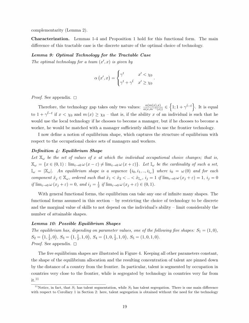
Lemma 10: Possible Equilibrium ShapesThe equilibrium has, depending on parameter values, one of the following five shapes: S

1

= (1, 0),S

2

=

�

1,

1

2

, 0

�

, S3

=

�

1,

1

2

, 1, 0

�

, S4

=

�

1, 0,

1

2

, 1, 0

�

, S5

= (1, 0, 1, 0).Proof. See appendix. �

The five equilibrium shapes are illustrated in Figure 4. Keeping all other parameters constant,the shape of the equilibrium allocation and the resulting concentration of talent are pinned downby the distance of a country from the frontier. In particular, talent is segmented by occupation incountries very close to the frontier, while is segregated by technology in countries very far fromit.11

11Notice, in fact, that S1 has talent segmentation, while S5 has talent segregation. There is one main differencewith respect to Corollary 1 in Section 2: here, talent segregation is obtained without the need for the technology

19

Proposition 4: Equilibrium Shapes and Distance to the FrontierLet S (d) be the equilibrium shape for a country at distance d =

¯

t� t from the frontier. There existfour constants d

1

< d

2

< d

3

< d

4

such that if ¯t� t d

1

, S (d) = S

1

; if ¯t� t 2�

d

1

, d

2

⇤

, S (d) = S

2

;if ¯t� t 2

�

d

2

, d

3

⇤

, S (d) = S

3

; if ¯t� t 2�

d

3

, d

4

⇤

, S (d) = S

4

; and if ¯t� t > d

4

, S (d) = S

5

.Proof. See appendix. �

Corollary 3: Concentration of Talent and Distance to the FrontierThe concentration of talent increases in the distance from the technology frontier.


Corollary 4: Conditions for Segregation and Segmentation in the Tractable Case(i) If ¯

t � t d

1

, talent is segmented by occupation; (ii) if ¯

t � t � d

4

, talent is segregated bytechnology.Proof. See appendix. �

A few features of Figures 4 and 5 are worth discussing.First, the equilibrium may dictate that some types x are indifferent between being managers or

workers – that is, w (x) = ⇡ (x) and w

0(x) = ⇡

0(x) (applying Lemma 4). How can ⇡

0(x) = w

0(x)

be satisfied? The slope of the matching function m (x) depends on the fraction of workers at x,! (x), and fraction of managers at m (x), 1�! (m (x)). The restriction w

0(x) = ⇡

0(x), therefore,

pins down the unique value of ! (x) in the indifference region. Second, just as in the general case,the skill-asymmetry parameter � plays an important role.12 The higher is �, the stronger thetask-complementarity is and, therefore, the lower the skill asymmetry. As a result, concentrationof talent increases in �. To visualize the role of � and d together, in Figure 5, I plot the contourplots of parameter values for which each equilibrium shape attains, as well as the correspondingvalues of the concentration of talent. Third, as the distance from the frontier (or, similarly,task complementarity) increases, the economic structure changes smoothly, in contrast to mostfrictionless matching models that feature a discrete jump between two polar cases.13 How does theequilibrium evolve as ¯

t� t increases? Consider the case with segmentation of talent in Figure 4a.When a country is sufficiently close to the technology frontier, the gap between the frontier and thelocal technology is small; thus, every team uses a similar technology and high-skilled individualsare assigned to be managers. As ¯

t � t increases, it becomes more rewarding for an individualto become a worker and get access to the frontier technology, rather than being a manager andusing the local vintage. The reward from being a manager rather than a worker depends also onthe production partner and, thus, on the matching function m. At first, only the lowest-skilledamong the managers finds it optimal to become workers. As ¯

t � t increases further, more andmore individuals who, if they were managers, would use local technology become workers in order

gap to go to infinite. This result is obtained because, in this limit case, the optimal technology function, ↵ (x0, x) is

not differentiable. Also notice that this result does not contradict Corollary 1 since Corollary 1 provides sufficientbut not necessary conditions for segregation and segmentation.

12With this functional forms, f1(x,m�1(x))f2(m(x),x) = 1+�m

�1(x)�m(x) that is decreasing in �.

13A CES production function provides a simple example of discrete jump in matching pattern: depending on thevalue of the elasticity of substitution it leads to either perfectly positive or perfectly negative assortative matching.

20

to get access to the frontier technology. When ¯

t � t is sufficiently large, access to the frontiertechnology drives the assignment. Therefore, the optimal allocation resembles a dual economy:within each technology, there is talent segmentation, but skills are segregated by technology.

Figure 4: Five Equilibrium Shapes(a) Segmentation, S1 = (1, 0) (b) S2 =

�

1, 12 , 0

�

(c) S3 =�

1, 12 , 1, 0

�

(d) S3 =�

1, 0, 12 , 1, 0

�

(e) Segregation, S5 = (1, 0, 1, 0)

Notes: the squared brackets put together individuals with the same occupation. Workers are highlighted with light greysquare brackets, and managers with black ones. Dotted brackets signal mixing: some are workers and some managers. Thered regions covers the set of individuals using the frontier technology vintage. The red striped regions represent mixing areas,in which the workers use the frontier technology, while the managers use the local technology. Dotted lines connect examplesof workers and managers that are together in a team.

Figure 5: Roles of Task Complementarity and Distance to the Frontier(a) Equilibrium Shape

2

2

2

2

3

3

3

3

4

4

5

5

10 20 30 40 50 60 70 80 90 100

Distance to the Frontier

10

20

30

40

50

60

70

80

90

100

Ta

sk-C

om

ple

me

nta

rity

(b) Concentration of Talent

0.5

0.5

0.5

0.5

0.5

25

0.525

0.525

0.525

0.5

5

0.55

0.55

0.55

0.5

75

0.575

0.575

0.575

0.6

0.6

0.6

0.6

0.6

25

0.625

0.625

0.625

0.6

5

0.65

0.65

0.65

0.675

0.675

0.675

0.7

0.7

0.7

0.725

0.725

0.725

0.75

0.75

0.75

10 20 30 40 50 60 70 80 90 100

Distance to the Frontier

10

20

30

40

50

60

70

80

90

100

Task-C

om

ple

menta

rity

Notes: the left figure shows the contour plots of the subsets of parameter values in the space of � (Task Complementarity)and d (Distance to the Frontier) for which each equilibrium shape attains. Specifically, the gray area highlights the set ofpairs (�, d) for which talent is segmented (S1). The line “2” then separates the region of S2 from the one of S1, and so onuntil the last shape, S5. The right figure shows the contour plots, in the same space, for the concentration of talent. Whentalent is segmented, the concentration of talent is equal to 0.5, its minimum value. When, instead, either d or � is sufficientlyhigh for talent not to be segmented, the concentration of talent increases smoothly in both parameters. Last, notice thatboth axes for � and d are normalized on a scale from 1 to 100, even though � only takes values in [0, 1] , and I use values ofd between 0 and 50.

21

3.3 Taking Stock: Some Insights for Economic DevelopmentIn this subsection, I summarize the theoretical insights that are of interest for economic de-

velopment. I also discuss how the empirical predictions of the model fit within the literature andthe role that cross-country differences in the distribution of skills may play.

Role of Team Production and Distance to the Frontier. Section 2 showed that theequilibrium allocation of talent and the cross-sectional distribution of technology are inherentlyintertwined. Section 3 further showed that the possibility to use the frontier technology vintages inless-developed countries leads them to larger technology dispersion and, consequently, to a differentallocation of talent. Specifically, in countries close to the technological frontier, most teams usea similar technology, and the allocation resembles the familiar structure from occupational choiceproblems: the low-skilled are workers and the high-skilled are managers. The main purpose ofteam production is to put together differently-skilled individuals to allow the most able ones tospecialize in the most skill-sensitive task. As a result, in countries close to the technologicalfrontier, all teams are fairly similar, and there is low productivity dispersion across them, whereasin countries far from the technological frontier, the allocation is asymmetric. Some teams attractskilled individuals (both managers and workers) and use frontier technologies, while others are leftwith low-skilled individuals and use traditional technologies. Teams now concentrate similarly-skilled individuals to reap the benefits of the complementarity between skills and technology. Asa result, there is larger dispersion of talent, technology, and productivity in the economy. Inthe limit case depicted in Figure 4e, the possibility of adopting frontier technology leads to anendogenous formation of a dual economy in poor countries. Teams that adopt advanced technologyattract the most-skilled individuals, leaving the rest of the economy with low talent, and, thuslower productivity.14 Theoretically, it is even possible that some individuals would use a highertechnology in autarchy than when countries gain access to the frontier, due to the polarizationof talent generated by the possibility of technology adoption. In fact, when talent concentrates,low-skilled workers are matched with lower-ability managers, and thus – ceteris paribus – woulduse a lower technology. For the same reason, technological leapfrogging is also possible in thisframework.

Empirical Predictions and Existing Literature. The model predictions on the economicstructure in developing countries are qualitatively consistent with a large body of empirical ev-idence. The larger productivity dispersion in poor countries has been noted by, among others,Caselli (2005), Hsieh and Klenow (2009), and Adamopoulos and Restuccia (2014). The modelalso predicts that in developing countries, some very low-skilled individuals are employed in man-agerial positions. Bloom and Van Reenen (2010) shows the existence of a thick left tail of poorlymanaged firms and that firms with more-educated manager have better management practices.More broadly, the asymmetric equilibrium resembles a dual economy, and duality is a featureoften associated with developing countries (see, for example, La Porta and Shleifer (2014)). Manyexisting theories that provide an explanation for these empirical facts attribute them to larger

14This feature resembles a mechanism outlined by Acemoglu (2015) (page 454) for the case of physical capital.

22

market frictions in developing countries. Instead, in the context of this paper, they emerge as aresult of differences in endowment that lead to differences in optimal allocations. This paper alsodeparts from the prior literature in linking these previously documented cross-country differencesto the different assignment of individuals to teams. Differences in the allocation of talent are anew feature of economic development that has been previously overlooked. In Section 4, I showthat it has empirical content.

Cross-Country Differences in Ability Distribution. The assumption that all countrieshave identical ability distribution – x ⇠ U [0, 1] – seems in contrast with the abundant empiricalevidence that average years of schooling are lower in poor countries. I intend x to capture therelative ability rank within a country, thus comparable only within countries and not across them.The reason for this choice is that there is an intrinsic isomorphism between the level of ability x

and the cost of technology. A higher ability is isomorphic to a lower cost of technology. Consideran example. Let h

t be a human capital term that captures the average ability of a country witha level of development t. Also, consider, for simplicity, the choice of technology for the tractablecase of Section 3.2. Keeping the cost of technology constant and letting ability change, is identicalto keeping ability fixed and letting the cost of technology change by a properly scaled factor:

max

a

axh

t � a

1+⌘

1 + ⌘

= max

a

ax� 1

h

(1+⌘)t

a

1+⌘

1 + ⌘

.

For this reason, the cross-country differences in the local technology vintage can be interpretedas cross-country differences in the level of human capital. I charge all cross-country differences tothe cost of technology for the sake of clarity.15

4 Empirical Evidence on the Allocation of Talent

I document cross-country differences in the allocation of talent.The main empirical challenge is to construct, for each country, a scalar statistic that summa-

rizes the information in the data on the allocation of talent. To directly compute the measure ofconcentration of talent defined in the model, we would need to observe the ability of all individ-uals in the economy and their production partners. Additionally, we would need such data to becomparable for several countries around the world. These ideal data do not exist.16

Therefore, in the main empirical exercise, I take an indirect approach that exploits one ofmodel’s assumptions: the complementarity between skills and technology. This assumption im-

15Allowing the distribution of ability to vary across countries would be more problematic. The reason is that thedistribution of ability may impact the matching patterns (See Kremer and Maskin (1996)). In a previous version ofthis paper (Porzio (2016)), I show that if individuals are allowed to invest in their ability – through schooling, forexample – then the distribution of schooling will depend on the matching pattern and the distribution of technology.The stronger concentration of talent and dispersion of technology in poor countries imply a larger cross-sectionaldispersion of education, as observed in the data.

16Matched employer-employee datasets are available for a few countries around the world. However, for less-developed countries, they are not representative of the whole economy.

23

plies that more-able teams use a more advanced technology. Observing the average ability ofindividuals that use each technology then becomes sufficient to make an inference on the match-ing function and, thus, the concentration of talent. In order to implement this strategy, we needan empirical measure of individual ability and the technology used. I use micro data from censusesand labor force surveys. In these data, I observe the education years and the working industry ofeach individual. I can then compute an empirical measure of concentration of talent under twoassumptions: (i) education is increasing in individual ability; and (ii) the industry in which anindividual works is a proxy for the technology that he uses. I will discuss potential concerns, butI first provide details on the data and on the exact construction of my empirical measure.

I also explore two alternative empirical strategies. In Section 4.5, using occupation data, Icompare the average ability of managers and workers across countries. In Section 4.6, using theavailable firm-level data, I compare the distributions of workers to firms across countries.

4.1 DataI use labor force surveys and censuses available from the Integrated Public Use Micro-data

Series, International (IPUMS). The data cover 63 countries of different income levels, from Rwandaand Tanzania to Switzerland and the United States. For most countries, the datasets have a verylarge sample. Merging all countries and years together, I have more than 600 million individuals.Some countries have larger datasets, but – in order to avoid comparability concerns – I extractfor each country-year pair a random sample of 500,000 individuals. For 13 countries, I have fewerthan 500,000 individuals, but for all countries I have at least 10,000 individuals that satisfy thesample selection criteria described. Part of my analysis focuses on the South Korean growthexperience, for which I use data from the Korean Longitudinal Study of Aging (KLoSA) and, toperform robustness checks, the Korean Labor and Income Panel Study (KLIPS). All GDP percapita data are taken from the Penn World Table version 8.0.

In the IPUMS data, there are three variables of interest: education, industry, and employmentstatus. Completed years of education is coded from the educational attainment variable, andindustries are standardized by IPUMS to be comparable across countries. Their industry definitionspans 12 industries. Employment status indicates whether an individual is a wage-worker, own-account self-employed or an employer. Following most of the literature, I restrict the sample toinclude males, head of households and those between 18 and 60 years old. For the baseline results, Ial exclude own-account self-employed since they do not work in teams. All data are representativeof the entire population from which they are drawn. Robustness checks and alternative sampleselections are in Section 4.4. Data details are in Appendix G.

KLoSA is a survey gathered with the purpose of understanding population aging in Korea.It has a sample size of approximately 10,000 individuals and represents individuals older than45. The survey, which started in 2006, is conducted biannually. Hence, it does not allow me todirectly trace the growth miracle in South Korea. However, a 2006 job supplement contains thecomplete employment history of each individual. In particular, this contains information on theindustry in which the respondent works, his employment status, and his education. Using thesedata, I retroactively construct cross-sections for each year from 1953 to 2006. There is one obvious

24

concern with this procedure: the average age of the individuals in my dataset changes over timeby construction, and, thus, I may confound life-cycle and time-series trends. Robustness checksin Appendix H address this concern.

Figure 6: Construction of the Measure of Concentration of Talent(a) Brazil, 2010

0.2

.4.6

.81

Ave

rag

e I

ndu

stry

Ed

uca

tion

0 .2 .4 .6 .8 1Industry Education in Perfect Sorting Case

Agriculture Manufacturing Services

(b) United States, 1940

0.2

.4.6

.81

Ave

rag

e I

ndu

stry

Ed

uca

tion

0 .2 .4 .6 .8 1Industry Education in Perfect Sorting Case

Agriculture Manufacturing Services

Notes: in each figure, I plot the average normalized measure of skills in an industry as a function of the average normalizedmeasure of skills in a counterfactual scenario in which there is perfect sorting of individuals across industries. Each dotcorrespond to an industry and the size of the dot is increasing in the number of individuals employed in that industry. Thedotted lines are the prediction from a linear regression weighted by the number of individuals in each industry. The slopesof the regression lines are the measures of the concentration of talent.

4.2 Measure of Concentration of TalentI build, separately for each country-year dataset, the empirical measure of concentration of

talent in five steps. First, I compute a normalized measure of skill: x

i

= F (s

i

), where s

i

denotesthe schooling years of individual i, and F is the country-year specific cumulative density function;to ease notation, I omit the country-year subscript, both here and in each of the following steps.17

Second, I compute the average skill in each industry j: ¯

x

j

= E [x

i

|Iij

= 1], where I

ij

is an indi-cator function equal to 1 if individual i works in industry j. Following the model assumption ofskill-technology complementarity, I interpret industries with higher average education as havinghigher technology.18 Third, I build a perfect sorting counterfactual in which talent is segregatedby technology. Specifically, keeping industry size constant, I assign all of the most-skilled indi-viduals to the industry with the highest average education, all the highest skilled ones amongthe remaining workforce to the second-highest and so on.19 Fourth, I compute the average skill

17The variable s takes a only finite number of values. Therefore, I renormalize x in such a way that the lowest-skilled individuals have ability x = 0 and the highest-skilled ones ability x = 1. Results are robust to alternatives.

18The ranking of industries is, by definition, country-year specific. However, most countries display a similarranking. For example, agriculture is consistently the less-skilled industry, while government is very high-skilled.

19Formally, let Xj

be the observed set of individuals in industry j, of mass v⇣

Xj

⌘

; then, ¯xj

= E

h

x|x 2 Xj

i

. The

counterfactual sets are given by Pj

⌘n

x : x 2h

P1 (j) , P2 (j)io

where P1 (j) ⌘P

k: ¯xk<¯xj

v

⇣

Xk

⌘

and P2 (j) ⌘

25

in each industry under the perfect sorting counterfactual: ¯

p

j

= E

h

x

i

|ICij

= 1

i

, where I

C

ij

is theconstructed indicator function. Fifth, and last, I regress ¯

x

j

= B

0

+ B

1

¯

p

j

+ " – weighting by thenumber of individuals in each industry. The measure of concentration of talent is ⇡ =

ˆ

B

1

. Bythe definition of the least squares estimator, ⇡ =

E

[

¯

x

j

�¯

x

j

0]

¯

p

j

�¯

p

j

0. ⇡ captures the expected ability gap

across industries relative to the benchmark case in which workers sort perfectly across industries.In Figure 6, I show two examples: Brazil in 2010 and United States in 1940. I plot the average

skill in an industry, ¯

x

j

, as a function of the skill in the perfect sorting counterfactual, ¯

p

j

. Eachdot in the figure corresponds to an industry, and its size increases in the number of individualsemployed in that industry. A linear regression ¯

x

j

= ↵+⇡

¯

p

j

+" fits the data well.20 Brazil in 2010had GDP per capita similar to that of the U.S. in 1940; however, it had a higher concentrationof talent (the regression line in the figure is steeper). This is consistent with the fact that Brazilin 2010 was farther from the technology frontier than the United States was in 1940. In Section4.3, I build this measure of concentration of talent for each country-year pair in my sample andsystematically document differences across countries depending on their distance from the frontier,but first, I further discuss its interpretation.

Link to the Model Definition of Concentration of Talent. The measure ⇡ captures howclose the observed allocation of talent is to the case in which individuals are perfectly sorted acrossindustries. Under the working assumption that industry can be used to proxy for technology used,we can interpret ⇡ as capturing how close the allocation of talent is to the case of segregation bytechnology. To fix ideas, consider that only two technologies are used: the local and the frontier.Assume, also, that we observe only two industries. As discussed, we measure ability with years ofeducation. Following the model, the industry with higher average education has a larger fractionof teams using the frontier technology. For simplicity, assume that all teams in this industry usethe frontier technology and that all teams in the other use the local technology.21 The argumentgeneralizes. Due to skill-technology complementarity, the most-skilled teams use the frontiertechnology and, hence, are in the same industry. But how are teams formed? Consider, first, thecase in which talent is segmented by occupation – that is, when talent concentration is low. Allmanagers are high-skilled, but some of them use the local technology and, thus, are in the low-technology industry. As a result, the ability gap across industries is small. Consider, next, the casein which talent is instead segregated by technology – that is, when talent concentration is high. Allof the most-skilled individuals now use the frontier technology, some of them being managers andother being workers. Only the lowest-skilled individuals are left in the low-technology industry.As a result, in this case, the ability gap across industries is, instead, large. Summing up, thisargument shows that the ability gap across industries captures how close the data are to eithersegregation by technology or segmentation by occupation.

P1 (j) + v

⇣

Xj

⌘

. Then, ¯p

j

= E

h

x|x 2 Pj

i

.20The average R

2 across countries from this regression is ⇠ 0.9 similarly in rich and poor countries.21This extreme assumption is not necessary, but we need that the set of teams in each industry to be connected;

that is, we cannot have both the very good and very bad teams select into the same industry. This is a still astrong assumption, but in 4.4 I discuss how the failure of it would likely bias my results downward.

26

Formally, I can show the equivalence between the empirical and theoretical measures of con-centration of talent under additional assumptions. Assume that there is a continuum of industries.Let a be the technology rank of an industry, by construction, a ⇠ U [0, 1]. Let x (a) be the averageability of individuals in a. Due to the definition of a, the counterfactual average ability is equal top (a) = a. The empirical measure of concentration of talent is given by the slope in the regressionof x (a) on a. Next, assume that the average ability of workers in a – call it x

w

(a) – can bewell approximated by a linear function with unknown slope: x

w

(a) = �a. Last, assume that theability gap between managers and workers is not correlated with technology. Under this set ofassumptions, the empirical measure of concentration of talent is equal to �. And we can see –using market clearing – that � is also identical to the model measure of concentration of talentdefined in 2.3:

1

2

1ˆ

0

x

w

(a) da+

1

2

1ˆ

0

x

m

(a) da =

1ˆ

0

xdx

1

4

� +

1

4

� +

1

2

1ˆ

0

[x

m

(a)� x

w

(a)] da =

1

2

� = 1�1ˆ

0

(m (x)� x)! (x) dx,

where I use the fact that´1

0

x

w

(a) da =

�

2

, and that – by market clearing and by the definition ofm (x) –

´1

0

x

w

(a) da =

´1

0

x! (x) dx and´1

0

x

m

(a) da =

´1

0

m (x)! (x) dx.

4.3 ResultsI now show that the concentration of talent varies systematically across countries as a function

of the distance to the technology frontier. Lemma 8 in Section 3, – which characterizes the rela-tionship between GDP per capita, the technology frontier and the country’s level of development– shows that there are three cross-country comparisons to identify differences in distance to thefrontier. First, compare two countries in the same year, but with different GDP per capita. Bothcountries face the same frontier; hence, the richer one is closer to the frontier. Second, comparetwo countries with the same GDP per capita, but in different years. Since the frontier grows overtime, the country observed in the past was closer to the frontier than the one observed today withthe same level of GDP per capita. Third, follow two countries over time. The one that growsfaster is approaching the frontier.

1

st Comparison: Poor and Rich Country Today. In Figure 7, I plot, for countries observedin the period 2000 to 2010, my measure of concentration of talent as a function of GDP percapita relative to that of the United States in 2010. Poor countries – i.e., those farther from thetechnology frontier – have larger concentration of talent. In order to interpret the magnitudeof cross-country differences, consider the following thought experiment. Let a country have twoindustries and two types of workers, high- and low-skilled. Both industries are of equal size, and

27

half of the population is high-skilled and half is low-skilled. If ⇡ in this economy is equal to 0,it means that half of the high-skilled individuals are in each industry. If ⇡ = 1, it means thatall the high-skilled individuals are in one industry, which I call the modern industry. If, instead,⇡ =

1

2

, 75% of the high-skilled are in the modern industry, and, hence, a high-skilled individual isthree times more likely to work in the modern industry. In this hypothetical world, the estimatesimply that high-skilled individuals in poor countries would be approximately five times as likelyto work in the modern industry as in the traditional one, while in rich countries, they would beonly twice as likely. In Section 5, I build a quantitative version of the model that allows me tofurther interpret the magnitude of these cross-country differences.

Figure 7: 1

st Comparison: Cross-county Differences in Concentration of Talent

LBR

MWI

RWA

UGA

SLE

TZA

MLI

SLV ZMB

KHM

CMR

IND

NGA

GHA

MNG

SDN

CHN

KGZ

VNM

BOL

IRQ IDN

PHL

MAR

JOR

EGY

JAM

ECU

FJI

PER

THA

LCA

ROU

COL

VEN

BRA

DOM

MYS

PAN

CRI

CHL

ARG

TUR

MEX

URY

IRN

HUN

PRT

GRC

ESP

SVN

ISRFRA

AUT

CAN

IRL

ITA

CHE

USA

.2.3

.4.5

.6.7

Conce

ntr

atio

n o

f T

ale

nt

.01 .025 .05 .1 .15 .3 .5 .75 1GDP pc Relative to the U.S. in 2010

Notes: light blue circles show how populated each country is. The dotted line is the fit from a regression of concentration oftalent on log of GDP per capita. The regression is not weighted by population since I treat each country as one observation.The regression line has a positive slope that is significant at the 1% level.

2

nd Comparison: Poor Countries Today and U.S. in the Past. We have usable censusdata for the United States every ten years from 1940 to 2010, since before the 1940 census, datadid not report education years. GDP per capita in the United States in 1940 is comparable tothat of many middle-income countries – such as Brazil, Mexico, Turkey, and Argentina – that Iobserve in my sample between 2000 and 2010. In fact, I observe 18 such countries and, amongthem, 16 have a higher concentration of talent than the U.S. used to have, as shown in Figure 8.22

This result alleviates the concern that the observed differences might be driven by differences inthe level of development rather than by the distance to the technology frontier.

3

rd Comparison: South Korea Convergence to the Frontier. Finally, I study the growthpath of South Korea, a particularly interesting country since it has converged to the frontier overthe past 50 years. South Korea’s GDP per capita relative to that of the United States increased

22I have computed a similar comparison for France, for which I have data to calculate the measure of concentrationof talent back to 1962. The results are very similar.

28

from only 7% to almost 60%. In Figure 9, I plot the growth path for concentration of talentacross sectors for both countries.23 U.S. concentration of talent remained fairly constant alongthe growth path, consistent with fact that the U.S. has been growing steadily over this period asa world leader – i.e., on the technology frontier. South Korea’s concentration of talent, instead,decreased steeply. This comparison alleviates the concern that cross-country differences might bedriven by time-invariant country characteristics that are correlated with GDP per capita.

Figure 8: 2

nd Comparison: Developing Countries today and U.S. in the past

United States, 1940

United States, 1950

JAM

VEN

THA

COL

ECU

PER

ROU

CRI

DOM

URY

BRA

CHL

ARG

MYSTUR IRN

PAN

MEX

.3.4

.5.6

.7C

once

ntr

atio

n o

f T

ale

nt

.1 .125 .15 .2 .27 .35GDP pc Relative to the U.S. in 2010

Notes: light blue circles show how populated each country is. The blue dotted line is at the level of concentration of talentof United States in 1940. A permutation test of the null hypothesis that the U.S. is not different from the other countriesrejects the null hypothesis more than 99% of the time.

Figure 9: 3

rd Comparison: South Korea as it Approaches the Frontier

1953195319531953

2006200620062006

1940

2010

.3.4

.5.6

.7C

once

ntr

atio

n o

f T

ale

nt

.025 .05 .1 .15 .25 .5 .75 1GDP pc Relative to the U.S. in 2010

United States South Korea

Notes: the figure shows the growth paths – over time – of the concentration of talent as a function of GDP.

23I use concentration of talent across sectors (hence aggregating industries to agriculture, manufacturing, orservices) because industry measure is not comparable for the United States and South Korea. Results with theconcentration of talent across industries are comparable.

29

4.4 RobustnessNext, I explore the robustness of the empirical results.The empirical strategy is sound if two assumptions hold: (i) individual ability and education

years are positively correlated; and (ii) individuals that work in higher-skilled industries use, onaverage, a more advanced technology. One concern is that the underlying patterns of matching areidentical across countries, and the observed differences are driven by mismeasurement resultingfrom the failure of one of the two working assumptions. I argue, however, that failures of theassumptions would most likely attenuate my results.

Assumption (i) allows me to measure skill using an individual’s years of education.24 Thereare few concerns. First, education might measure skill with white noise.25 This is not a problem,however. Since I compare average skill by sector, measurement error does not bias the results:because there are a large number of individuals within each sector, this type of measurementerror washes out. Second, the documented cross-country patterns can be observed if individualsare similarly matched on ability in all countries; and in poor countries, more-able individualshave more education, while in rich countries, the relationship between education and skills is non-monotonic. This hypothesis seems at odds with the often made claim that in developing countries,schooling choices are more constrained. (See, for example, Mestieri (2016)).

Assumption (ii) allows me to measure technology using the industry in which an individualworks. Specifically, according to my interpretation, if an industry has a more educated work-force, it should have a more advanced technology. This is consistent with the model’s predictionthat more-skilled teams sort into higher production technologies. It is also consistent with theprevious literature that argues that some sectors use technologies with a higher degree of skillcomplementarity (see, for example, Buera et al. (2015)) and that documents large productivitygaps across sectors in developing countries (see, for example, Caselli (2005), Gollin et al. (2014),and Acemoglu and Zilibotti (2001) ). Nonetheless, one concern remains: my results will be bi-ased if industry is a worse proxy for technology in countries closer to the frontier. My empiricalresults can be obtained in an hypothetical scenario in which individuals are identically matchedin all countries, but in rich countries, dispersion of technology within industries is larger than inpoor ones. This seems at odds with empirical evidence that documents, even in narrowly definedindustries, larger dispersion of productivity in poor countries (see, for example, Hsieh and Klenow(2009) and Asker et al. (2014)).

Next, I explore robustness to alternative sample selections or measures of concentration oftalent. All the results are reported in Table 1, which I refer to below, focusing on the cross-sectional comparison.

24A prominent alternative measure of skills is individual income. I choose to use education years for three reasons:(i) in most countries, only wage income is available, and only a fraction of the developing country workforce receivesa formal wage; (ii) even when non-wage income data are available, they are hard to compare with wage incomesince they might capture non-individual returns (e.g., family labor); (iii) income measures are available only for asubset of countries.

25I use education to make an ordinal comparison across individuals within a country. As a result, any cross-country comparability concern is alleviated. For example, the concern of Hanushek and Woessmann (2008) – i.e.,that cross-country education differences understate those in cognitive ability – does not apply.

30

Table 1: Robustness TablePoint Estimate R

2

(1) Baseline -0.0708 36.3%Level of Industry Aggregation

(2) Sectors (Agr, Mfg, Ser) -0.0861 44.0%(3) Unharmonized Industries -0.0472 17.3%

Sample Selection(4) Include Non Households Heads -0.0681 35.5%(5) Include Women -0.0719 37.9%(6) Only Women -0.0610 15.0%(7) Include Self-Employed (Own-Accounts) -0.0715 36.4%

Role of Agriculture(8) Drop Agriculture -0.1710 55.3%(9) Only Individuals non in Agriculture -0.0266 8.7%

Measure of Concentration of Talent(10) Correlation -0.0407 24.9%(11) Correlation Using Normalized Skills -0.0246 10.3%

Notes: The point estimates are from the cross-country regressions of the concentration of talent on log of GDP per capita. All

Coefficients are significant at less than 1%, with the exception of rows (9) and (11) that are significant at less than 5%.

First, I explore alternative definitions of industries. I aggregate industries at the sector level(agriculture, manufacturing, services), or I use, when available, a finer definition of industries.This second alternative comes at the cost of a lack of cross-country comparability since the levelof aggregation varies. The results are robust (rows 2 and 3).26

Second, I explore alternative sample selections. Results are robust to the inclusion of malenon-household heads (row 4), or females (row 5). I then restrict the sample to only females(row 6). The fit is weaker, but the point estimates are significant and similar. Last, I includeown-account self-employed: the result does not change (row 7).

Third, I investigate whether the results are driven mainly by the prevalence of agriculture indeveloping countries.27 I address this point through two exercises. I start by recomputing themeasure of concentration of talent, dropping agricultural industries in the previously describedcross-industry regression used to compute ⇡ – i.e., ¯

x

j

= B

0

+ B

1

¯

p

j

+ ". Row 8 shows that thelarger measure in poor countries does not come purely from the gap between agriculture andnon-agriculture, but, rather, holds also within other sectors. I then consider only individuals whoare not in agriculture and recompute both the normalized measure of skill and the concentrationof talent. This exercise calculates cross-country differences in concentration of talent if, suddenly,all individuals in agriculture were to drop out of the labor force. The results (row 9) are weakerand smaller in magnitude but still show more concentration in poor countries.

Fourth, and last, I compute an alternative measure of concentration of talent, along the lines26Examples of Brazil 2010 and the United States 1940 are in Figures A.7 and A.8 in the Appendix G. We can

appreciate that the nice fit of the measure of concentration of talent is present at any level of aggregation.27The comparison between currently poor countries and the U.S. in the past already hinted towards the fact that

the result cannot be driven solely by differences in agricultural share, since – Herrendorf et al. (2014) show – mostcountries follow a structural transformation pattern similar to that of the U.S. in the past.

31

of the one used in Kremer and Maskin (1996) – namely, the correlation between individuals’education and the average education in an industry:

⇡

2

= Corr (sij

,E (s

i

|Iij

= 1)) .

Also under this alternative measure, which is equivalent to a variance decomposition exercise,poor countries have a stronger concentration of talent. The results hold both if computed withraw education (row 10) or with normalized skills x (row 11).

4.5 Evidence from Occupation DataIPUMS data report information on individual occupations, coded following the International

Standard Classification of Occupations (ISCO). ISCO occupations do not correspond to the notionof managers and workers in my model. ISCO’s definition of occupations seems to depend onthe technology used: a manager that uses a backward technology would likely not be coded asa manager but, rather, as someone in an “elementary occupation.” In fact, the occupation ofmanager, according to ISCO, is an occupation with skill level 4. The ISCO report, available atilo.org, states: “Occupations at this skill level (4) generally require extended levels of literacy andnumeracy, sometimes at very high level . . . and typically involve the performance of tasks thatrequire complex problem-solving, decision-making and creativity based on an extensive body oftheoretical and factual knowledge . . .” A manager of a low-technology firm in a developingcountry – who should be coded as a manager according to my model – does not fit well into thisdefinition. As a result, I cannot directly use the ISCO definition of a managers to provide supportfor the model. Instead, I follow two alternative approaches.

First, from the data, I build two variables that most closely resemble the model’s definition ofmanagers and workers. I code as managers individuals who are either managers according to theISCO definition or who report being self-employed. Managers of high-technology firms are likelycoded as ISCO-managers, while those at low-technology firms – which are often small, privatelyowned, and informal – are most likely captured in the data as self-employed. I code as workers allother employed individuals: they are wage workers and not managers according to ISCO. I thencalculate, in each country, the average rank in the education distribution (my empirical measureof ability x) for managers and workers. Recall that the measure of concentration of talent ina country is given by 1 minus the average ability distance between a worker and his manager,1 �´(m (x)� x)! (x) dx, where ! (x) is the probability that individual x is a worker. Using

market clearing, I can write

1�ˆ

(m (x)� x)! (x) dx

| {z }

Concentration of Talent

= 1�ˆ

x (1� ! (x)) dx

| {z }

Average Manager Ability

+

ˆx! (x) dx

| {z }

Average Worker Ability

.

The model predicts that in poor countries, the concentration of talent is higher. Therefore, weshould observe that the average ability of workers is higher in poor countries and that the average

32

ability of managers is lower. This prediction is supported in the data, as shown in Figure 10.28

Figure 10: Broad Occupation Categories

(a) Workers

SLV

LBR

MWI

TZA

ZMBCMR

KHM

GHA

FJIPHLMAR

BOL

IND

IRQJAM

PRY

JOR

MNG

EGY

ARM

ECU

PER

THA

BRADOM

VEN

MYSIRNMEXPAN

ROU

CHL

TUR

HUN PRT

GRC

ESPITA

FRAGBRCANAUTNLD

IRL

USA

.4.5

.6.7

.8.9

Ave

rage E

duca

tion R

ank


(b) Managers

SLV

LBR

MOZ

SLE

MWI TZA

ZMBCMR

KHM

GHA

FJI

PHLMARBOL

IND

IRQ

JAMPRY

JOR

MNG

EGY

ARMECU

PERTHA

BRADOMVEN

MYSIRN

MEX

PANROU

CHL

TUR

HUN

PRT

SVN

GRC

ESPITA

FRA

GBR

CANAUT

NLDIRL

USA

.4.5

.6.7

.8.9

Ave

rage E

duca

tion R

ank


Notes: light blue circles show how populated each country is. Regression lines are not weighted by population size.

This first approach has one main limitation: the definitions of workers and managers maybe not comparable across countries. Therefore, I take a second route and focus on narrowlydefined occupations. In the data, an occupation is often a bundle task-technology. The model’soccupation-technology29 trade-off suggests that occupations that entail simple tasks (and, thus,would correspond to workers in the model) but use an advanced technology should be performedby relatively more skilled individuals in poor countries. Cashiers in retail stores seems to bean appropriate example. Within my model, retail cashiers are “workers” who use an advancedtechnology: they perform a relatively simple task within their team, working below a store orchain manager, but use an advanced technology, the cash register. Retail cashiers are comparableacross countries and easy to identify in the data.30 Moreover, they usually do not own thetechnology they use, which alleviates the concern that the results might be driven by bindingcredit constraints in poor countries. I compute average years of schooling and normalized skillsof retail cashiers in each country. Figures 11a and 11b show that – consistent with the model– retail cashiers are relatively more skilled in poor countries.31 Of course, there is a degree of

28The average ability of managers is only slightly lower in poor countries. This is driven by two counteractingforces. The ISCO-managers are more skilled in poor countries, while the self-employed are less skilled. On net,managers are slightly less skilled in poor countries. This additional piece of evidence shows that there is a largerdispersion of skills among managers in poor countries, consistent with the model’s predictions.

29The model’s definition of “occupation” corresponds more closely with a task, rather than with an occupation,in the data.

30In almost all countries, the codebooks for the unharmonized occupation variable encompass the categorycashier. The industry variable then allows me to identify retail cashiers. Specifically, I call an individual a retailcashier if he has the variable INDGEN = 60, and he is coded as cashier in the unharmonized occupation variable(OCC in IPUMS. Cashiers are identifiable from the codebooks available for each country). I managed to code retailcashiers for 54 countries. Beware that in some countries, there are few retail cashiers. In fact, the median countryhas 30 observations, and the minimum number of observations is five.

31I can also confirm that the results are not driven by selection into retail by looking at the education of retailmanagers, as previously defined. Figures A.11a and A.11b show that retail managers are only mildly more skilledin poor countries.

33

arbitrariness in the choice of occupation to focus on. Another possible alternative could be to usedrivers of motor vehicles. Driving is a simple task, and a motor vehicle is an advanced technology.Figures 11c and 11d show that – again, as predicted – drivers are relatively more skilled in poorcountries.

Figure 11: Narrow Occupation Categories: Retail Cashiers and Motor Vehicle Drivers

(a) Average Education of Retail Cashiers

SLVLBR

MOZ

SLE

MWI

UGA

TZA

RWA

ZMB

CMR

KHM

GHA

VNM

FJI

PHL

MAR

BOL

IND

IRQJAM

PRY

JOR

MNGEGY

ARM

ECU

PER

THA

BRADOM

VEN

MYS

IRN

MEXPANROU

CHL

TURHUN

PRT

SVNGRC

ESP

ITA

FRA

CAN

AUTIRL

USA

05

10

15

Years

of E

duca

tion


Overall Average Average of Cashiers in Retails

(b) Education Rank of Retail Cashiers

SLVLBR

MOZ

SLE

MWI

TZA ZMBCMR

KHM

GHA

FJI

PHL

MAR

BOL

IND

IRQ

JAM

PRY

JOR

MNGEGY

ARM

ECU

PER

THABRA

DOM

VEN

MYS

IRN

MEX

PAN

ROU

CHL

TUR

HUN PRT

SVN

GRC

ESP

ITA

FRAGBR

CAN

AUTNLD

IRL

USA

.4.5

.6.7

.8.9

Ave

rage E

duca

tion R

ank


(c) Average Education of Motor Vehicle Drivers

SLV

MOZ

GINMLI

UGA

RWA

SEN

ZMB

CMRKHM

SDN

VNM

FJI

PHL

MAR

BOL

IND

IRQ

JAM

PRY

JOR

MNG

ARM

ECU

PER

THA

BRADOM

VEN

MYS

IRNMEX

PANCHL

HUN

PRT

GRCITA

FRA

AUT

USA

05

10

15

Years

of E

duca

tion


Overall Average Average of Motor Vehicle Drivers

(d) Education Rank of Motor Vehicle Drivers

SLV

MOZ

ZMB

CMR

KHM

FJI

PHL

MARBOL

IND

IRQ

JAM

PRY

JOR

MNG

ARM

ECUPER

THA

BRADOMVEN

MYSIRN

MEXPAN

CHL

HUN PRTGRCITA

FRA

GBR

AUT

USA

.3.4

.5.6

.7.8

Ave

rage E

duca

tion R

ank


Notes: light blue circles show how populated each country is. Regression lines are not weighted by population size.

4.6 Evidence from Firm DataThe World Bank Enterprise Surveys provide firm-level information from several countries

around the world. Specifically, they report the average education of workers and managers inthe firm, and measures of technology and labor productivity. Unfortunately, these data sufferfrom major cross-country comparability concerns; as noted by Asker et al. (2014), for example.Most importantly, they cover only registered firms, which constitute a much larger fraction of thelabor share in rich countries. Despite these concerns, these data can be used to provide furthervalidation for the model. I do so in detail in Appendix E. I interpret a team in the model as a

34

firm in the data. The three main findings are as follows. First, I validate the main prediction ofthe assumptions of skill-technology and manager-worker complementarity. I show that, similarlyin rich and poor countries, more-educated workers are employed in firms with higher technology(measured by computer usage), higher labor productivity, and better-educated managers. Second,I show that, consistent with Proposition 3, dispersion of used technology across firms is largerin less-developed countries. Third, I show that talent, measured as years of education, is moreconcentrated within firms in less-developed countries, as suggested by Corollary 2.

5 A Quantitative Exploration

As discussed in Section 3.3, the equilibrium in countries far from the technology frontier, de-spite being efficient, predicts several empirical features that are usually attributed to the presenceof larger frictions in developing countries. In view of this result, cross-country exercises that com-pare micro-level allocations should be cautious in assigning all the observed differences to largerfrictions in developing countries.

In this section, I take a first step in understanding whether the mechanism that this paperproposes could be quantitatively relevant in explaining cross-country differences. I ask whetherthe model can explain a sizable fraction of the larger agricultural productivity gaps documentedin poor countries (see Caselli (2005)). Specifically, I write down a version of the model that isamenable to a quantitative exploration of the data. Next, I estimate it using data on the allocationof talent in rich and poor countries and the agricultural productivity gap in rich countries. I thenshow that, once fitted into the model, the observed cross-country differences in allocation of talentreconcile approximately one third of the larger agricultural productivity gaps in poor countries.

5.1 Quantitative ModelI add one feature to the model in Section 2. Each individual is characterized not only by his

ability x, but also by a vector of technology-specific shocks, which make him more willing to usesome technologies rather than others. The introduction of this additional source of noise allowsme to develop an efficient numerical algorithm and to make the model amenable for estimation.Apart from this feature, the quantitative model mirrors the one presented in Section 2.

Each individual x chooses the technology that gives him the highest value. He solves

max

a2A�

a

y (a, x) ,

where A = {a1

, .., a

N

} is a discrete approximation of the set of available technologies; �

a

isdistributed according to a Frechet with dispersion parameter ✓ (dispersion of shocks increases as✓ decreases)

�

a

⇠ e

��

�✓

a

;

and y (a, x) is the income of an individual of ability x that uses technology a and picks his

35

occupation optimally

y (a, x) = max

z2[0,1]z⇡ (a, x) + (1� z)w (a, x) .

Managers choose the optimal worker among the set ⌦a

that gathers the individuals that are usingtechnology a:

⇡ (a, x) = max

z2⌦a

g (a, x, z)� w (a, z) . (3)

The Spence-Mirrlees assumption (Assumption 3 in Section 2) guarantees that, as long as individu-als use the same technology, the most-skilled ones are managers. Market clearing dictates that themass of manager and workers for each technology should be identical. These two conditions allowme to solve – given � (a, x), which is the joint distribution of individuals over technology a andability x – for the cutoff types x (a) that characterize the occupational choice in each technology:

x(a)ˆ

0

� (a, x) dx =

1ˆ

x(a)

� (a, x) dx.

The income of an individual x that uses technology a is then given by

y (a, x) =

8

<

:

w (a, x) if x x (a)

⇡ (a, x) if x > x (a).

The matching function within each technology, m (a, x), is derived using the fact that, due tothe complementarity of f , there is positive assortative matching between managers and workers.m (a, x) solves for all (x, a)

m(a,x)ˆ

x(a)

� (a, z) dz =

xˆ

0

� (a, z) dz.

Wages and profits are calculated using the first-order and envelope conditions of the manager’sproblem (3), together with market clearing ⇡ (a,m (x))+w (a, x) = af (m (x) , x)� c (a). That is,

w (a, x) = +

xˆ

0

w

2

(a, z) dz

⇡ (a, x) = w (a, x (a)) +

xˆ

x(a)

⇡

2

(a, z) dz,

36

where satisfies

x(a)ˆ

0

w (a, x)� (a, x) dx+

1ˆ

x(a)

⇡ (a, x)� (a, x) dx =

x(a)ˆ

0

g (a,m (a, x) , x)� (a, x) dx.

The properties of the Frechet distribution (see, for example, Hsieh et al. (2016)) provide a simpleequation that characterizes, together with market clearing, the distribution of individuals overtechnologies, � (a, x). Specifically, the probability that an individual x selects into technology a

is

� (a, x)

P

a2A � (a, z)

=

y (a, x)

✓

P

a2A y (a, x)

✓

, (4)

where y (a, x) = max {0, y (a, x)}. Last, the GDP per capita is

Y =

X

a2A

x(a)ˆ

0

g (a,m (a, x) , x)� (a, x) dx. (5)

This model can be computed for any functional form for net output g – hence, for f and c –that satisfies the assumptions in Section 2. The computing algorithm iterates on the distribution� (a, x) until convergence. Details are in Appendix F. The numerical solution is fast, thus allowingme to estimate the model through a simulated method of moments, as I discuss next.

5.2 Model EstimationI next describe how I estimate the model. Six steps are involved. First, I pick parsimonious

functional forms that give five parameters to be structurally estimated. Second, I describe thetargeted moments in the data. Third, I show how to construct equivalent moments in the model.Fourth, I provide some details on the estimation method. Fifth, I show the fit of the model andthe external validation exercises. Sixth, I comment on the identification of the parameters.

Functional Forms and Parameters. I need to pick a functional form for net output g –hence, for f and c. I choose parsimonious functional forms to limit the number of parameters tobe estimated. I use f (x

0, x) = x

0(1 + �x), where � 2 [0, 1] modulates the strength of the gap in

skill sensitivity between managers and workers: @

@�

f1(x,y)

f2(y,z)< 0, for all (x, y, z). � 1 guarantees

that the Spence-Mirrlees condition is satisfied. For the cost of technology, I use c (a; t,

¯

t), asdefined in Lemma 5 in Section 3. c (a; t,

¯

t) is modulated by three main parameters: (i) ⌘, thecost elasticity within technology vintages; (ii) ", the cost elasticity across technology vintages;and (iii) �

0

, the level of the cost of importing foreign technology vintages. Additionally, I fixthe non-homotheticity term ⌫ equal to 1, just as in the tractable case of Section 3.2, and I fix� = 1.02, which corresponds to 2% yearly growth at the frontier. The value of � does not affectthe results since it is not separately identified from ¯

t and t. Intuitively, two years away from thefrontier at 2% growth per year is the same as one year away at 4.04% growth per year. As I

37

showed in Section 3, only the distance to the frontier, ¯t� t, matters for the technology gaps andthe allocation of talent: thus, I can fix ¯

t without loss of generality. I choose ¯

t such that a countryon the frontier – hence, with t =

¯

t – has the level of GDP per capita of the United States.Summing up, the production function g gives four parameters to be estimated, three for c

and one for f . Additionally, we have the new parameter ✓, which modulates the dispersion ofthe technology shocks. Therefore, I estimate five parameters within the model. Given the vectorof these parameters, I can compute the equilibrium for countries at different distances to thefrontier – i.e., for different values of t – and study how the allocation of talent and agriculturalproductivity gaps vary as a function of GDP per capita.

Data Moments. I target three sets of moments: (i) the empirical relationship between GDPper capita and concentration of talent; (ii) the agricultural productivity gap in countries closeto the frontier; (iii) the percentage of agricultural workers by skill level in countries close to thefrontier. For (i), I use the empirical results of Section 4, and, specifically, I target the values ofconcentration of talent as a function of log GDP predicted by the regression line in Figure 7. For(ii), I use the average agricultural productivity gap – i.e., the ratio between labor productivity innon-agriculture and agriculture – for the first quartile of GDP per capita, as reported in Gollin etal. (2014). For (iii), I compute the fraction of workers in agriculture, separately for different skillbrackets, using the same IPUMS data as described in Section 4. For each country, I compute thenormalized measure of skills x, just as described in 4, and calculate for each skill decile the fractionof people that work in agriculture. I then divide the countries in my dataset into four groups tomatch the average GDP of the four quartiles of Gollin et al. (2014) – the first one has GDP percapita that is 78% of the United States’; the second 21%; the third 8.7%; and the fourth 2.5% –and take the average within each group. The result of this procedure is shown in Figure 12b: richcountries have a smaller fraction of workers in agriculture, and in all countries, low-skilled peopleare more likely to work in agriculture. These result are consistent with evidence in the previousliterature; see, for example, Caselli (2005) and Caselli and Coleman (2001).

Model Moments. First, notice that the equilibrium objects described in Section 5.1 are func-tions of the vector of parameters, which I define ⇥ ⌘ {⌘, ",�

0

,�, ✓}, and the level of developmentt. I now make this dependence explicit in my notation. For example, I use Y (t,⇥) for GDP percapita, defined in equation (5), rather than simply Y .

I treat the model-generated data following the same procedure that I used for the micro data,and according to the same assumptions. I next describe in detail how I construct the moments.

For a given vector of parameters ⇥, I first find ˆ

t such that Y

(

ˆ

t,⇥

)

Y (

¯

t,⇥)

= 1%, where Y (

¯

t,⇥) isthe GDP per capita of the United States. I then compute the model for 100 countries withequally spaced values of t in

⇥

ˆ

t,

¯

t

⇤

. The result is a model-generated dataset of 100 countries withGDP per capita between 1% and 100% of that of the frontier – i.e., the United States. Foreach country t 2

�

ˆ

t, ...,

¯

t

, I compute the relative GDP per capita: Y (t,⇥)

Y (

¯

t,⇥)

. I then divide the setof 100 countries into four groups such that their average relative GDP per capita matches thefour quartiles from Gollin et al. (2014). That is, I create T

1

=

�

ˆ

t, ..., t

k1

, T2

= {tk1+1

, ..., t

k2},

38

T3

= {tk2+1

, ..., t

k3}, T4

= {tk3+1

, ...,

¯

t} such that 1

|T1|P

k1j=1

Y (t

j

,⇥)

Y (

¯

t,⇥)

= 2.5%, 1

|T2|P

k2j=k1+1

Y (t

j

,⇥)

Y (

¯

t,⇥)

=

8.7%, 1

|T3|P

k3j=k2+1

Y (t

j

,⇥)

Y (

¯

t,⇥)

= 21%, 1

|T4|P

100

j=k3+1

Y (t

j

,⇥)

Y (

¯

t,⇥)

= 78%. These quartiles are useful later.To calculate the concentration of talent, I use the procedure described in Section 4, but with

model-generated data. I keep the assumption that an industry is a technology, and I calculate theaverage ability of individuals that use each technology a

x (a; t,⇥) =

´1

0

x� (a, x; t,⇥) dx´1

0

� (a, x; t,⇥) dx

.

I then calculate the counterfactual average ability under perfect sorting

p (a; t,⇥) =

a�1X

a=a1

2

4

1ˆ

0

� (a, x; t,⇥) dx

3

5

+

´1

0

� (a, x; t,⇥) dx

2

,

where a�1

is the technology just worse than a. The measure of concentration of talent, which Icall ⇡m

(t,⇥), is given by the coefficient ˆ

�

1

from the regression x (a; t,⇥) = �

0

+ �

1

p (a; t,⇥) + ".I next need to define a notion of agriculture in the model. In all countries, agriculture is

the industry with the lowest average education. Therefore, following the assumptions of Section4, I construct agriculture in the model as the partition of teams that use the least-advancedtechnologies. I choose such a mass of teams to match the agricultural employment in the datafor the countries in the same quartile of GDP. Agriculture is, thus, the partition of teams thatproduce with technologies in the set Aagr

(t,⇥) = {a1

, .., a

n

}, where a

n

is such that32

X

a2Aagr

(t,⇥)

1ˆ

0

� (a, x; t,⇥) dx ' L

agr

(t) ,

and if country t is in quartile x – i.e., t 2 Tx

– then L

agr

(t) =

ˆ

L

agr

x

, where ˆ

L

agr

x

is the averageshare of employment in agriculture measured in the IPUMS data for countries in the x

th quartile.Output in agriculture and non-agriculture is, thus, given by

Y

agr

(t,⇥) =

X

a2Aagr

(t,⇥)

x(a;t,⇥)ˆ

0

g (a,m (a, x; t,⇥) , x; t,⇥)� (a, x; t,⇥) dx (6)

Y

nagr

(t,⇥) =

X

a2Anagr

(t,⇥)

x(a;t,⇥)ˆ

0

g (a,m (a, x; t,⇥) , x; t,⇥)� (a, x; t,⇥) dx, (7)

where Anagr

(t,⇥) = A\Aagr

(t,⇥) = {an+1

, ..., a

N

}. The agricultural productivity gap, Z (t,⇥),is simply, as in the data, the ratio between the labor productivity in non-agriculture and in

32Since A is a discrete set, in general, there is no a

n

such that this equation holds with exact equality. Forsufficiently large |A|, the approximation error is small. To avoid any concern, I find a

n

and then randomly assign toagriculture a fraction of teams of the closest technology in such a way that the model exactly matches the fractionof agricultural workers.

39

agriculture; that is,

Z (t,⇥) =

Y

nagr

(t,⇥)

L

nagr

(t)

Y

agr

(t,⇥)

L

agr

(t)

.

Finally, the fraction of people employed in agriculture by skill level is

⇢ (x; t,⇥) =

P

a2Aagr

(t,⇥)

� (a, x; t,⇥) dx

P

a2A(t,⇥)

� (a, x; t,⇥) dx

.

Estimation Method. For a given vector of parameter ⇥, I compute the following measure ofthe distance between the model and the data

L (⇥) =

1

100

100

X

j=1

✓

⇡

m

(t

j

,⇥)� ⇡

d

(t

j

)

⇡

d

(t

j

)

◆

2

+

1

10

10

X

s=1

✓

⇢

m,1

(x

s

;⇥)� ⇢

d,1

(x

s

)

⇢

d,1

(x

s

)

◆

2

+

✓

Z

m,1

(⇥)� Z

d,1

Z

d,1

◆

2

where a few objects have not been defined yet: ⇡

d

(t

j

) is the targeted empirical value of theconcentration of talent for a country t

j

; ⇢

m,1

(x

j

;⇥) is the average fraction of individuals witha skill level in decile s that are employed in agriculture for the model-generated countries inthe first quartile – i.e., ⇢

m,1

(x

s

;⇥) =

1

|T1|P

t2T1⇢ (x

s

; t,⇥); ⇢

d,1

(x

s

) is the same object in thedata; Zm,1

(⇥) is the average agricultural productivity gap for countries in T1

– i.e., Zm,1

(⇥) =

1

|T1|P

t2T1Z

m

(t,⇥); and Z

d,1 is the corresponding empirical value from Gollin et al. (2014). Theestimated vector of parameters is ⇥

⇤= argminL (⇥). To solve this minimization problem, I

use the simulated method of moments. Specifically, I simulate, using the Metropolis–Hastingsalgorithm, a Markov chain that converges to the vector of parameters that minimizes the distancebetween the model and the data.33

Model Fit and Validation. The model fits the data fairly well. Figure 12a shows the cross-country relationships between concentration of talent and GDP per capita in the model and inthe data. The dotted line represents the targeted values, ⇡d, while the red crosses are the model-generated data, ⇡

m

(·,⇥⇤). Figure 12b shows agricultural employment by skill, separately for

each GDP quartile. The targeted data, ⇢d,1, are the points of the darkest line. The model data,⇢

m,1

(·,⇥⇤), are the darkest crosses. The model matches the average agricultural employment by

construction, but the estimation targets the heterogeneity by skills. The model’s and the data’sagricultural productivity gaps, Zm,1

(⇥

⇤) and Z

d,1, respectively, are shown in rows (4) and (7) ofthe first column of Table 2.

I also provide two validation exercises. First, notice that in Figure 12b, the relationships be-tween skills and agricultural employment for GDP quartiles 2, 3, and 4 are not targeted. Nonethe-less, the model matches these empirical relationships. Second, and more remarkably, the modelpredicts well the share of individuals in each country that use the frontier technology vintage. Iconstruct, using the CHAT dataset (Comin and Hobijn (2009)), the number of internet users per

33For details on the simulated method of moments, see McFadden (1989). The simulation method that I use wasdeveloped first by Chernozhukov and Hong (2003) and was recently used in Lise et al. (2016).

40

capita for several countries in 2005, when the world wide web was arguably a frontier technology.The relative fraction of internet users across the world should correspond to the model’s relativefractions of individuals that use the frontier vintage.34 I plot the data along with the model’spredictions in Figure 12c.

Figure 12: Model Fit and Validation

(a) Concentration of Talent

LBR

MWI

RWA

SLE

TZA

MLI

UGA

SLV ZMB

KHMCMR

IND

NGA

GHA

MNG

SDN

CHN

KGZ

VNM

BOL

IRQ

PHL

IDN

MAR

JOR

EGY

JAM

ECU

FJI

PER

THA

LCA

ROU

COL

VEN

BRA

ARGDOM

MYS

PAN

CRI

CHL

TUR

URY

MEX

IRN

HUN

PRT

GRC

ESP

SVN

ISRFRA

AUT

CAN

IRL

ITA

CHE

USA

.2.3

.4.5

.6.7

Co

nce

ntr

atio

n o

f T

ale

nt


(b) Ability Distribution in Agriculture

02

55

07

51

00

Pe

rce

nta

ge

Em

plo

yed

in A

gricu

lture

0 .25 .5 .75 1Ability Rank

Rich Middle Income Poor Very Poor

(c) Penetration Rate of Internet Users

UGA

TZA

KEN

BGD

SDN

PAK

VNM

IND

PHL

MAR

IRQ

IDN

EGY

UKR

CHNCOL

ZAF

THA

BRA

IRN

MEXARGTURRUS

POL

KOR

ESP

ITA

JPN

FRA

GBRDEUCANUSA1.2

5.1

.01

.00

3In

tern

et

Use

rs R

ela

tive

to

th

e U

.S.

in 2

00

5


Notes: the top left panel plots the empirical measure of concentration of talent, calculated as described in Section 4, and the

same statistic computed in the model (red crosses) as a function of relative GDP per capita. The top right panel shows the

average fractions of people employed in agriculture as a function of their skills, separately for the four quartiles of GDP per

capita. The solid lines are the data. The crosses are the values computed in the model. The bottom panel plots the fraction – in

2005 – of internet users relative to the U.S., calculated from the CHAT dataset together with the relative fraction of individuals

– computed in the model – that use the frontier technology vintage (red crosses) as a function of relative GDP per capita. In

this same figure, the black dotted line is the fit line (of relative internet users on relative GDP per capita) for 2005, while the

gray dotted line is the fit line of the same regression but with data from 2010.

34Internet users captures only the extensive margin and not the intensive margin of technology usage. I’vecomputed similar results for other technologies in the CHAT dataset, such as number of computers, and number ofcell phones. The results look similar but are harder to interpret because they confound the number of users withthe amount of technology per person.

41

Model and data align fairly well. The model, however, slightly overestimates the fraction ofinternet users relative to the data. In the same figure, I also plot the empirical relationship for2010. The model underestimates the relative fraction of internet users when compared to 2010.This is consistent with the world wide web becoming less of a frontier technology over the period2005 to 2010.

Comments on Identification. The five parameters are jointly determined by the targetedmoments. Nonetheless, I discuss intuitively the main links between moments and parameters.� decreases the skill asymmetry, hence increases the concentration of talent. ⌘ decreases thetechnology gap for teams that use the same technology vintage, hence decreases the concentrationof talent. Additionally, ⌘ affects the agricultural productivity gap since a higher ⌘ implies a loweragricultural gap for a given team composition. In countries close to the frontier, ⌘ and � arethe main determinants of the concentration of talent since most teams use the same vintage.Therefore, � and ⌘ together are relevant mainly in matching the concentration of talent andagricultural productivity gap close to the frontier. " affects how much the concentration of talentincreases as a function of the distance from the frontier. In fact, the higher is ", the costlier it is forcountries with a low local technology vintage to upgrade to the next available vintage. As a result,the higher is ", the more similar are the technologies used and the lower is the concentration oftalent. �

0

affects the cost of importing technology vintages and, thus, the mass of people in eachcountry that decide to not use the local technology. The higher is �

0

, the higher the decrease inGDP as we decrease the level of development t. Therefore, " and �

0

together match mainly therelationship between the change in concentration of talent and the change in GDP per capita.Last, the dispersion of technology shocks ✓ mainly pins down how many high-skilled individualswork in agriculture relative to non-agriculture. Consider that high-skilled individuals have, ceterisparibus, a comparative advantage in advanced technology. Therefore, if we observe many of themin agriculture, it must be that the dispersion of the technology shock is large, thus pushing manyhigh-skilled into agriculture.

5.3 Results on Agriculture Productivity GapsI next use the estimated model to study the extent to which the larger agricultural productivity

gaps in poor countries are driven by the interaction of the endogenous allocation of talent and thepossibility of importing advanced technology from the frontier. I compute the model-generatedagricultural productivity gap for each quartile of the income distribution – that is, Zm,x

(⇥

⇤) =

1

|Tx

|P

t2Tx

Z

m

(t,⇥

⇤) for x 2 {1, 2, 3, 4} – and compare them with the empirical ones reported in

Gollin et al. (2014). Results are in rows (4) and (7) of Table 2. The model, once disciplined bycross-country differences in the concentration of talent, reconciles a sizable amount, approximatelyone third, of the higher agricultural productivity gap in developing countries.35 Therefore, a naivecross-country comparison that takes as null the hypothesis that the agricultural productivity gapshould be identical, would overstate the extent to which market frictions are larger in developingcountries. At the same time, even after accounting for endogenous technology choice and team

35The value 13 is calculated as follows: the total increase in the data from the first to the fourth quartile is

3.6 = 5.6� 2; the same value in the model is, instead, 1.3 = 3� 1.7; and 1.33.6 ' 1

3 .

42

formation, more than half of the cross-country differences remain unexplained, thus still leavinga prominent role to larger market failures in developing countries or to any other competitiveexplanations that are not present in this model.

Role of Endogenous Allocation of Talent. The role of endogenous allocation of talent istwofold. First, it permits me to discipline the model: the predicted larger agricultural productivitygaps in poor countries are modulated by their larger empirically measured concentration of talent.In fact, if I estimate the model targeting identical concentration of talent in all countries, then thepredicted agricultural productivity gaps are similar across countries – the remaining differencesare driven by the country-specific mass of people employed in agriculture – and actually slightlysmaller in countries far from the frontier. Second, the larger concentration of talent in countriesfar from the frontier amplifies their larger productivity dispersion. I explore the quantitativerelevance of this amplification mechanism by computing counterfactual agricultural productivitygaps in a scenario in which all countries have the output function g of the average country inthe first quartile, but retain their country-specific concentration of talent. That is, I replaceg (a,m (a, x; t,⇥

⇤) , x; t,⇥

⇤) with g

�

a,m (a, x; t,⇥

⇤) , x;

¯

t

1

,⇥

⇤�, where ¯

t

1

=

1

|T1|P

t2T1t, when I

calculate agricultural and non-agricultural outputs using equations (6) and (7), and then I usethese value to calculate the agricultural productivity gaps. The results are shown in row (8)of Table 2. The allocation of talent alone explains almost 40% of the difference in agriculturalproductivity between the first and the fourth quartiles.36

Table 2: Allocation of Talent and Agriculture to Non-Agriculture Productivity Gaps

Quartiles of World Income DistributionQ1 Q2 Q3 Q4

(1) GDP pc Relative to U.S. 78% 21% 8.7% 2.5%

Data(2) Concentration of Talent 38% 47% 53% 62%(3) Internet Users Relative to U.S. 79% 28% 9% 2%(4) Agricultural Productivity Gap 2 3.2 3.4 5.6

Model

(5) Concentration of Talent 40% 57% 61% 63%(6) Internet Users Relative to U.S. 92% 41% 16% 2%(7) Agricultural Productivity Gap 1.7 2 2.4 3(8) Productivity Gap with Fixed g 1.7 1.7 1.8 2.2

36Notice that while the concentration of talent increases between quartiles 1 and 2, the agricultural productivitygap does not increase significantly. Why does this happen? Recall that the agricultural productivity gap depends,in this counterfactual, only on the skills of people in agriculture and in non-agriculture. In quartiles 1 and 2, a smallfraction of the overall population works in agriculture. As a result, although the concentration of talent increasesdue to changes within non-agriculture, these changes are not sufficiently large to sizably affect the agriculture tonon-agriculture gap.

43

Robustness. In order to explore whether the results are robust to perturbations around thevalue of ⇥⇤, I compute the agricultural productivity gaps averaged across other “good fit” parame-ter sets from the chain simulated for the estimation. Specifically, letting H =

n

⇥ :

L(⇥)�L(⇥⇤)

L(⇥⇤)

< 1%

o

,

I compute ¯

Z

m,x

=

1

|H|P

⇥2H

h

1

|Tx

|P

t2Tx

Z

m

(t,⇥)

i

, for x 2 {1, 2, 3, 4}. This exercise gives:¯

Z

m,1

= 1.8, ¯

Z

m,2

= 2.1, ¯

Z

m,3

= 2.7, ¯

Z

m,4

= 3.6. The results are, therefore, similar and, ifanything, stronger than those for the point estimate ⇥

⇤.

6 Extensions of the Analytical Model

The main theoretical insight of this paper is that the allocations of talent and technologyare intertwined due to a technology-occupation trade-off. This insight – once extended to richerframeworks – may have a variety of additional predictions. In this section, I informally discussedtwo directions that I explored: introducing self-employment, and dynamics.

We might also be concerned about the robustness of the occupation-technology trade-off toa richer framework in which managers are allowed to choose firm size. I here show that – understronger assumptions on the skill-technology complementarity – the trade-off is robust.

Self-Employment. I extend the tractable framework of Section 3.2 allowing individuals tochoose whether to produce alone or in teams. Details and empirical results are in Appendix B. Imodel self-employment along the lines of Garicano and Rossi-Hansberg (2004): it is an occupationmore skill-intensive than a worker, but less than a manager. As a result, when everyone uses asimilar technology, as in countries close to the technology frontier, the self-employed are just asskilled as the average individual. However, selection into self-employment is different in countriesfar from the technology frontier. I show that the farther a country is from the technology frontier,the more negatively selected the self-employed are. Intuitively, in countries far from the frontier,low-skilled individuals become self-employed because the types that would be their managers in acountry close to the frontier choose to be workers themselves to get access to advanced technology.In this sense, the model provides an equilibrium explanation for the prevalence of subsistence self-employment in poor countries, a phenomenon widely documented in the literature (e.g., Schoar(2010), Ardagna and Lusardi (2010) and Banerjee and Duflo (2012)). I also use the same datasetdescribed in Section 4 to document that, consistent with model’s predictions, own-account self-employed workers are relatively less skilled in countries far from the frontier.

Growth, Time of Take-off, and Dual Economy Traps. The benchmark model is static.Individuals live one period, and everyone faces identical costs of technology. I next discuss analternative setting, in which individuals still live one period, but the technology they use survivesthem and can be used by individuals in next period. In this setting, we need to define an allocationmechanism to assign existing technologies to teams. One possibility is to use a competitivemethod and let teams bid for existing technologies. This mechanism leads to positive assortativematching – due to skill-technology complementarity – between the technologies and the skills ofteam’s managers. Each team can also decide whether to further improve their assigned technology.

44

Countries differ with respect to the exogenous time in which they take off and start importingtechnologies from the frontier. Before that, everyone in the country uses the local technologyvintage, which does not improve over time. The frontier technology grows exogenously. Consider,first, a country that takes off early. The frontier technology vintage is still similar to the localvintage. As a result – just as in the static model – there is little technology dispersion, and talentis segmented by occupation. In the periods after the take-off, the better-skilled teams match withthe best existing technology, but technology dispersion is contained, and, thus, talent remainssegmented by occupation, and the whole economy grows at similar rate. Consider, instead, acountry that takes off late. The frontier technology vintage had evolved, while the local onedid not. As a result, the country is far from the frontier, and this leads – just as in the staticmodel – to talent segregation by technology: high-skilled individuals pair together and adoptthe most advanced technologies. Technology dispersion builds up in the economy, thus favoringfurther talent segregation. Segregation can be beneficial in the short run, concentrating talent andpushing some parts of the economy to quickly converge to the frontier. At the same time, though,it may lead to dual economy traps since other parts of the economy are crowded out of talentand, thus, have weak incentives to adopt the advanced technology. In this case, reallocating high-skilled workers towards more depressed parts of the economy – towards rural areas, for example– may be beneficial to long run growth.

Firm Size. In the benchmark model, a manager has only one way to leverage his talent: to hire amore-skilled worker. Managers are, in fact, not allowed to hire more than one worker. In AppendixD, I show that this restriction can be relaxed while still preserving the core theoretical insights. Istudy the marginal values of skills for managers and workers when managers can choose the firmsize. Endogenous firm size does play a relevant role, but as long as we assume a stronger degreeof complementarity between skills and technology – specifically, log-super-modularity rather thansuper-modularity, along the lines of results in Grossman et al. (2017) – the technology-occupationtradeoff is still present and so is the role of the cost of technology in shaping the assignment oftalent.

7 Conclusion

This paper develops a theoretical framework for studying the link between the allocationof talent into production teams and the cross-sectional distribution of technology. The theoryhighlights that the main purpose of team production and, thus, the equilibrium assignment oftalent depends on the distance of a country from the technology frontier. In countries close tothe frontier, all teams use a similar technology, and the main purpose of team production is togather together high- and low-skilled individuals to allow for task specialization. In contrast,in countries far from the frontier, the main purpose of team production is to match individualswith their appropriate production technology. As a result, high-skilled individuals gather togetherin teams that adopt the most advanced technology, while the low-skilled are left to match with

45

one another and use backward technology. The theoretical predictions are supported by cross-country micro data on the allocation of talent. Moreover, a quantitative analysis demonstratesthat the observed cross-country differences in the allocation of talent can account for a sizablefraction of larger productivity dispersion in poor countries. Thus, the model suggests that weshould be cautious about assigning all the observed cross-country differences to larger frictions indeveloping countries, as is often done in the extensive literature that studies the (mis)allocation ofresources in developing countries. Through the lens of the theory here proposed, those exercises aremisspecified because they do not take into account the endogenous team formation and technologychoice.

More broadly, this paper brings attention to a new feature of economic development thathas been previously overlooked: individuals in poor countries form production teams differentlythan those in rich countries. This paper focuses on the implications of this phenomenon forcross-sectional productivity dispersion. However, the cross-country differences in “who matcheswith whom” may matter for several other core questions of economic development. For example,the different patterns of matching may influence the formation of social networks, or the degreethrough which information and knowledge spread out within an economy, thus ultimately affectingthe growth rate of a country.37

37Specifically, a recent literature (e.g., Lucas and Moll (2014), Perla and Tonetti (2014), and Buera and Oberfield(2016)) develops theoretical models in which growth is generated through the diffusion of ideas. If embedded withinthese models, the different patterns of assignment in developing countries would affect the overall speed of learningand possibly generate a trade-off between the allocation of talent that maximizes output and the one that maximizestechnology diffusion. Evidence of slow accumulation of human capital over the life-cycle, which might be driven byslow learning due to lack of interaction of individuals of different skills, is documented in Lagakos et al. (2017).

46

ReferencesAcemoglu, Daron, “Changes in Unemployment and Wage Inequality: An Alternative Theory

and Some Evidence,” American Economic Review, 1999, pp. 1259–1278.

, “Localised and Biased Technologies: Atkinson and Stiglitz’s New View, Induced Innovations,and Directed Technological Change,” The Economic Journal, 2015, 125 (583), 443–463.

and Fabrizio Zilibotti, “Productivity Differences,” Quarterly Journal of Economics, May2001, 116 (2), 563–606.

, Philippe Aghion, and Fabrizio Zilibotti, “Distance to Frontier, Selection, and EconomicGrowth,” Journal of the European Economic association, 2006, 4 (1), 37–74.

Adamopoulos, Tasso and Diego Restuccia, “The Size Distribution of Farms and InternationalProductivity Differences,” The American Economic Review, 2014, 104 (6), 1667–1697.

Ardagna, Silvia and Annamaria Lusardi, “Explaining International Differences in En-trepreneurship: The Role of Individual Characteristics and Regulatory Constraints,” in “In-ternational Differences in Entrepreneurship,” University of Chicago Press, 2010, pp. 17–62.

Asker, John, Allan Collard-Wexler, and Jan De Loecker, “Dynamic Inputs and Resource(Mis)Allocation,” Journal of Political Economy, 2014, 122 (5), 1013–1063.

Atkinson, Anthony B and Joseph E Stiglitz, “A New View of Technological Change,” TheEconomic Journal, 1969, pp. 573–578.

Banerjee, Abhijit and Esther Duflo, Poor economics: A Radical Rethinking of the Way toFight Global Poverty, PublicAffairs, 2012.

Basu, Susanto and David N Weil, “Appropriate Technology and Growth,” Quarterly Journalof Economics, 1998, pp. 1025–1054.

Ben-Porath, Yoram, “The Production of Human Capital and the Life Cycle of Earnings,”Journal of Political Economy, 1967, 75, 352.

Bloom, Nicholas and John Van Reenen, “Why Do Management Practices Differ Across Firmsand Countries?,” The Journal of Economic Perspectives, 2010, pp. 203–224.

Bloom, Nick and John van Reenen, “Measuring and Explaining Management Practices AcrossCountries and Firms,” Quarterly Journal of Economics forthcoming, 2007.

Buera, Francisco J and Ezra Oberfield, “The Global Diffusion of Ideas,” Technical Report,National Bureau of Economic Research 2016.

, Joseph P Kaboski, and Richard Rogerson, “Skill Biased Structural Change,” TechnicalReport, National Bureau of Economic Research 2015.

Caselli, Francesco, “Technological Revolutions,” American economic review, 1999, pp. 78–102.

, “Accounting for Cross-Country Income Differences,” in Philippe Aghion and Steven Durlauf,eds., Handbook of Economic Growth, Vol. 1, Elsevier, 2005, chapter 9, pp. 679–741.

and Wilbur John Coleman, “The U.S. Structural Transformation and Regional Conver-gence: A Reinterpretation,” Journal of Political Economy, 2001, 109 (3), 584–616.

47

Caunedo, Julieta and Elisa Keller, “Capital Obsolescence and Agricultural Productivity,”Cornell University Working Paper, 2016.

Chernozhukov, Victor and Han Hong, “An MCMC Approach to Classical Estimation,” Jour-nal of Econometrics, 2003, 115 (2), 293–346.

Chiappori, Pierre-André, Alfred Galichon, and Bernard Salanié, “The Roommate Prob-lem is More Stable than you Think,” 2014.

, Robert J McCann, and Lars P Nesheim, “Hedonic Price Equilibria, Stable Matching,and Optimal Transport: Equivalence, Topology, and Uniqueness,” Economic Theory, 2010, 42(2), 317–354.

Comin, Diego A and Bart Hobijn, “The CHAT Dataset,” Technical Report, National Bureauof Economic Research 2009.

and Martí Mestieri, “If Technology Has Arrived Everywhere, why Has Income Diverged?,”Technical Report, Darmouth College Working Paper 2016.

Eeckhout, Jan and Philipp Kircher, “Assortative Matching with Large Firms: Span of Controlover More versus Better Workers,” Universitat Pompeu Fabra Working Paper, 2012.

Feenstra, Robert C, Robert Inklaar, and Marcel P Timmer, “Penn World Table Version8.0,” The Next Generation of the Penn World Table, available for download at www. ggdc.net/pwt, 2013.

Foster, Andrew D and Mark R Rosenzweig, “Technical Change and Human-Capital Returnsand Investments: Evidence from the Green Revolution,” The American economic review, 1996,pp. 931–953.

Garicano, Luis and Esteban Rossi-Hansberg, “Inequality and the Organization of Knowl-edge,” American Economic Review, 2004, pp. 197–202.

and , “Organization and Inequality in a Knowledge Economy,” The Quarterly Journal ofEconomics, 2006, 121 (4), 1383–1435.

Gennaioli, Nicola, Rafael La Porta, Florencio Lopez de Silanes, and Andrei Shleifer,“Human Capital and Regional Development*,” The Quarterly journal of economics, 2013, 128(1), 105–164.

Goldin, Claudia and Lawrence F Katz, “The Origins of Technology-Skill Complementarity*,”The Quarterly journal of economics, 1998, 113 (3), 693–732.

Gollin, Douglas, David Lagakos, and Michael E. Waugh, “The Agricultural ProductivityGap,” Quarterly Journal of Economics, 2014, 129 (2), 939–993.

Grossman, Gene M, Elhanan Helpman, and Philipp Kircher, “Matching and Sorting ina Global Economy,” Journal of Political Economy, 2017, 125 (1).

Hanushek, Eric A and Ludger Woessmann, “The Role of Cognitive Skills in EconomicDevelopment,” Journal of economic literature, 2008, pp. 607–668.

Herrendorf, Berthold, Richard Rogerson, and Ákos Valentinyi, “Growth and StructuralTransformation,” Handbook of Economic Growth, 2014, 2, 855–941.

48

Hsieh, Chang-Tai and Peter J. Klenow, “Misallocation and Manufacturing TFP in Chinaand India,” Quarterly Journal of Economics, 2009, 124 (4), 1403–1448.

, Erik Hurst, Charles I. Jones, and Peter J. Klenow, “The Allocation of Talent and U.S.Economic Growth,” Stanford Working Paper 2016.

Kremer, Michael, “The O-ring Theory of Economic Development,” The Quarterly Journal ofEconomics, 1993, pp. 551–575.

and Eric Maskin, “Wage Inequality and Segregation by Skill,” Technical Report, NationalBureau of Economic Research 1996.

Lagakos, David, “Explaining Cross-Country Productivity Differences in Retail Trade,” Journalof Political Economy, 2016, 124 (2), 579–620.

and Michael E Waugh, “Selection, Agriculture, and Cross-Country Productivity Differ-ences,” American Economic Review, 2013, 103 (2), 948–80.

, Benjamin Moll, Tommaso Porzio, Nancy Qian, and Todd Schoellman, “Life-CycleWage Growth Across Countries,” Journal of Political Economy, 2017, (Forthcoming).

Lise, Jeremy, Costas Meghir, and Jean-Marc Robin, “Matching, Sorting and Wages,”Review of Economic Dynamics, 2016, 19, 63–87.

Lucas, Robert E. and Benjamin Moll, “Knowledge Growth and the Allocation of Time,”Journal of Political Economy, 2014, 122 (1), 1 – 51.

Lucas, Robert E Jr., “On the Size Distribution of Business Firms,” Bell Journal, 1978, 9,508–523.

McFadden, Daniel, “A Method of Simulated Moments for Estimation of Discrete ResponseModels without Numerical Integration,” Econometrica, 1989, pp. 995–1026.

Mestieri, Martí, “Wealth Distribution and Human Capital: How Do Borrowing ConstraintsShape Educational Systems,” Technical Report, Northwestern Working Paper 2016.

Minnesota Population Center, Integrated Public Use Microdata Series, International: Version6.1 [Machine-readable database], University of Minnesota, 2011.

Perla, Jesse and Christopher Tonetti, “Equilibrium Imitation and Growth,” Journal of Po-litical Economy, 2014, 122 (1), 52 – 76.

Porta, Rafael La and Andrei Shleifer, “Informality and Development,” The Journal of Eco-nomic Perspectives, 2014, pp. 109–126.

Porzio, Tommaso, “Distance to the Technology Frontier and the Allocation of Talent,” YaleUniversity Working Paper, 2016.

Roys, Nicolas and Ananth Seshadri, “Economic Development and the Organization of Pro-duction,” Technical Report, University of Wisconsin Madison Working Paper 2014.

Schoar, Antoinette, “The Divide between Subsistence and Transformational Entrepreneurship,”in “Innovation Policy and the Economy, Volume 10,” University of Chicago Press, 2010, pp. 57–81.

49

Suri, Tavneet, “Selection and Comparative Advantage in Technology Adoption,” Econometrica,2011, pp. 159–209.

Young, Alwyn, “Inequality, the Urban-Rural Gap and Migration*,” The Quarterly Journal ofEconomics, 2013, p. qjt025.

50

Cross-Country Diﬀerences in the Optimal Allocation of ...

Documents

Transcript of Cross-Country Diﬀerences in the Optimal Allocation of ...