Clemson UniversityTigerPrints

All Dissertations Dissertations

8-2008

MODELING SYSTEMS FOR OPTIMALRESOURCE ALLOCATION, SCHEDULING,AND DECISION MAKINGEsengul TayfurClemson University, etayfur@clemson.edu

Follow this and additional works at: https://tigerprints.clemson.edu/all_dissertations

Part of the Industrial Engineering Commons

This Dissertation is brought to you for free and open access by the Dissertations at TigerPrints. It has been accepted for inclusion in All Dissertations byan authorized administrator of TigerPrints. For more information, please contact kokeefe@clemson.edu.

Recommended CitationTayfur, Esengul, "MODELING SYSTEMS FOR OPTIMAL RESOURCE ALLOCATION, SCHEDULING, AND DECISIONMAKING" (2008). All Dissertations. 259.https://tigerprints.clemson.edu/all_dissertations/259

MODELING SYSTEMS FOR OPTIMAL RESOURCE ALLOCATION,

SCHEDULING, AND DECISION MAKING

A Dissertation

Presented to

the Graduate School of

Clemson University

In Partial Fulfillment

of the Requirements for the Degree

Doctor of Philosophy

Industrial Engineering

by

Esengul Tayfur

August 2008

Accepted by:

Dr. Kevin M. Taaffe, Committee Chair

Dr. Ronnie A. Chowdhury

Dr. William G. Ferrell

Dr. Mary Elizabeth Kurz

ii

ABSTRACT

This dissertation focuses on the resource requirements and scheduling problem for

logistic systems. We investigate solutions to this problem in two different logistic

systems: logistic system of the health care facilities during emergency evacuations and

delivery and distribution system of production industries.

All hospitals must have an evacuation plan to ensure the safety of patients and

prevent the loss of life. However, hospital operators have not been able to quantify how

resource availability, the cost of acquiring those resources, and evacuation completion

time are related. This research addresses this problem and contributes two methodologies

to solve this problem.

In the first methodology, we propose a mixed integer programming for identifying

resource requirements, as well as the scheduling of these requirements, within a pre-

specified period while minimizing cost. Also, we suggest a tailored solution approach

that relaxes certain complicating integer constraints in an effort to find feasible, quality

solutions. This model assumes that there exists no probabilistic event in the evacuation

process of the hospitals. The second proposed methodology accounts for uncertainties in

the evacuation process. We present a stochastic model via simulation and employ a

simulation-optimization approach to solve the same problem.

The resource requirements and scheduling problem is also a critical issue for the

companies in the production industry as most of them have limited resources and need to

make their tactical and operational plans with the consideration of this issue. As the

iii

focus of this dissertation is logistic operations, we consider this problem only for the

logistic system of these companies and contribute methodologies to solve this problem.

With the use of same structure of the formulation, used in mixed integer programming

proposed for the evacuation problem, we propose models to solve this problem for two

different production environments: when there is no limitation on resources and when

there are limited resources. The models proposed for the restricted production

environment also enables the companies to select the most profitable set of customers.

We also suggest tailored solution approaches for each model with the use of the same

techniques used for evacuation planning problem.

iv

DEDICATION

I dedicate this dissertation to my mother, Ayse Tayfur.

v

ACKNOWLEDGMENTS

I would like to thank my advisor, Dr. Kevin M. Taaffe for his guidance

throughout this research. I also would like thank to my committee members, Dr. Ronnie

A. Chowdhury, Dr. William G. Ferrell, and Dr. Mary Elizabeth Kurz for their valuable

advice.

Finally, I would like to express my deepest gratitude to my family, who has

always believed in me and supported me throughout my life. I would not be able to

accomplish this achievement without them.

vi

TABLE OF CONTENTS

Page

TITLE PAGE .................................................................................................................... i

ABSTRACT ..................................................................................................................... ii

DEDICATION ................................................................................................................ iv

ACKNOWLEDGMENTS ............................................................................................... v

LIST OF TABLES ........................................................................................................ viii

LIST OF FIGURES ......................................................................................................... x

CHAPTER

I. INTRODUCTION ......................................................................................... 1

II. LITERATURE REVIEW .............................................................................. 8

Introduction .............................................................................................. 8

Hospital Evacuation Planning in case of Hurricane Event ...................... 8

Delivery and Distribution Systems ........................................................ 12

III. AN OPTIMIZATION MODEL FOR ALLOCATING AND

SCHEDULING RESOURCES

DURING HOSPITAL EVACUATIONS .............................................. 20

Introduction ............................................................................................ 20

Methodology .......................................................................................... 21

Experimentation .................................................................................... 31

Weighted Time Objective ...................................................................... 47

Concluding Remarks .............................................................................. 50

IV. SIMULATING HOSPITAL EVACUATION – THE INFLUENCE OF

TRAFFIC AND EVACUATION TIME WINDOWS .......................... 52

Introduction ............................................................................................ 52

Background ............................................................................................ 53

Methodology .......................................................................................... 55

Experimentation ..................................................................................... 62

vii

Table of Contents (Continued)

Page

Concluding Remarks .............................................................................. 82

V. RESOURCE ALLOCATION AND CUSTOMER SELECTION

FOR PERIODIC DELIVERY AND DISTRIBUTION PROBLEM ..... 84

Introduction ............................................................................................ 84

Methodology ......................................................................................... 85

Experimentation .................................................................................... 98

Concluding Remarks ............................................................................ 117

VI. CONCLUSIONS AND RECOMMENDATIONS .................................... 118

Conclusions .......................................................................................... 118

Recommendations ............................................................................... 121

APPENDICES ............................................................................................................. 123

1: Optimization Result Tables........................................................................ 124

2 : Optimization Result Tables for Cases with Fixed Costs ........................... 160

3: Optimization Result Tables for Weighted Time Objective ....................... 164

4: Evacuation Decision Flowchart ................................................................. 174

5: Analysis for Effects of Number of Simulations ......................................... 175

6: Simulation Optimization Result Tables for

Different Target Evacuation Times ..................................................... 178

7: Simulation Optimization Result Tables of Cases with Fixed Costs .......... 184

8: Simulation Optimization Result Tables for

Different Evacuation Start Times Before Landfall .............................. 185

9: Simulation Optimization Result Tables of Cases with Fixed Costs

for Different Evacuation Start Times Before Landfall ........................ 191

10: Heuristic Result Tables of [DDM] ............................................................. 192

11: Optimal Result Tables of [RSCSDDM] .................................................... 194

12: Heuristic Result Tables of [RSCSDDM] ................................................... 196

13: Integrality and Optimality Gaps of Cases

with Restricted Storage Space ............................................................. 200

14: Optimal Result Tables of [RBCSDDM] .................................................... 201

15: Heuristic Result Tables of [RBCSDDM] .................................................. 203

16: Integrality and Optimality Gaps of Cases with Restricted Budget ............ 207

REFERENCES ............................................................................................................ 208

viii

LIST OF TABLES

Table Page

3.1 Cost of nurses for different target evacuation times .................................... 33

3.2 Values of [10P ,

20P ,30P ] for all test cases ..................................................... 34

3.3 Cases resulting in optimal solutions with the [HEM] .................................. 36

3.4 Performance of heuristic approach for various target evacuation times ...... 37

3.5 Effects of nurse restrictions (24-hour target evacuation time)..................... 40

3.6 Solution capability using a weighted time objective ................................... 48

3.7 Comparison of cost and weighted time objective ........................................ 49

4.1 Time distributions of each process (by patient type) ................................... 63

4.2 Cost of nurses for different target evacuation times .................................... 67

4.3 Cost of a transporting nurse for evacuation start time ................................. 68

4.4 Half widths of time in system performance measure................................... 69

4.5 Number of replications found from both approaches .................................. 70

4.6 Analysis for number of replications ............................................................. 71

4.7 Analysis for number of simulations ............................................................. 72

4.8 Results for 3 shelters when varying the target evacuation time................... 74

4.9 Results for 15 shelters when varying the target evacuation time ................. 75

4.10 Results for 3 shelters when varying the evacuation start time ..................... 78

4.11 Results for 15 shelters when varying the evacuation start time ................... 79

4.12 Influence of evacuation start time on evacuation completion time ............. 81

5.1 Mapping of decision variables and data parameters .................................... 90

ix

List of Tables (Continued)

Table Page

5.2 Cases resulting in optimal solutions with the [DDM] ............................... 101

5.3 Integrality Gaps .......................................................................................... 103

5.4 Optimality Gaps ......................................................................................... 103

5.5 Sample Results Obtained from Heuristic [DDM] ...................................... 105

5.6 A few cases resulting in optimal solutions

with [DDM] and [RSCSDDM] ............................................................ 109

5.7 Sample Results Obtained from Heuristic [RSCSDDM] ............................ 111

5.8 A few cases resulting in optimal solutions

with [DDM] and [RBCSDDM] ........................................................... 114

5.9 Feasibility analysis for budget ................................................................... 116

x

LIST OF FIGURES

Figure Page

3.1 Cumulative nurse requirements for a case

with three sheltering facilities ................................................................ 38

3.2 Cumulative vehicle requirements for a case

with three sheltering facilities ................................................................ 41

3.3 Staging nurse requirements for different target evacuation times ............... 42

3.4 Transporting nurse requirements for different target evacuation times ....... 43

3.5 Vehicle requirements for different target evacuation times ......................... 43

3.6 Cost (structure 1) vs. target evacuation completion time (in hours) ............ 44

3.7 Cost (structure 2) vs. target evacuation completion time (in hours) ............ 46

4.1 A simulation optimization model (Carson and Maria (1997)) ..................... 55

4.2 Behavioral response curves, S-curve (see FEMA (1986-2006)) ................. 59

4.3 Traffic factors over evacuation time horizon ............................................... 66

4.4 Cost values of base case versus target evacuation time ............................... 76

4.5 Cost values of alternate case versus target evacuation time ........................ 77

4.6 Cost values of base case versus evacuation start times ................................ 79

4.7 Cost values of alternate case versus evacuation start times ......................... 80

5.1 Profit analyses with same demand distributions ........................................ 106

5.2 Budget analyses with same demand distributions ..................................... 106

5.3 Profit and budget analyses for two-product delivery type

with different demand distributions ..................................................... 107

5.4 Profit analyses with same demand distributions

when space is restricted ....................................................................... 112

xi

List of Figures (Continued)

Figure Page

5.5 Profit analyses with two-product delivery type with different

demand distributions when space is restricted ..................................... 112

1

CHAPTER ONE

INTRODUCTION

There are a lot of examples in which logistics systems modeling plays a critical

role in identifying infrastructure requirements and determining improved methods for

moving goods or people across a constrained system. In many situations, we need to

consider positioning of resources, whether they come in the form of materials and

inventory, or in terms of people and staff.

In this research, we focus on finding the allocations and schedules of the

resources for logistics operations aimed to be achieved within a pre-specified period of

time while considering monetary objectives. We carry out the research with two different

types of logistics systems: logistics system of the health care facilities during emergency

evacuation (Chapter 3 and 4) and delivery and distribution system of production

industries (Chapter 5).

Although these systems seem distinctively different, they have many similarities.

Both of the systems have restrictions on the number and capacity of the resources.

Different types of objects are transferred to different locations via different types of

vehicles and resources are used to stage the objects on the vehicles in both of the systems.

In both systems, there exist contracts with logistic companies that enable them the

flexibility on the number of vehicles to lease.

On the other hand, the major difference between these two systems is that patients

are staged onto the vehicles with the help of nurses and are transferred to the sheltering

2

facilities during the evacuation of the health care facilities, whereas products are loaded

onto the vehicles by material handlers and delivered to the customers in the production

industries. Also, evacuation of the patients occurs very rarely, while delivery of the

products is a very frequent activity for the production companies. For the logistic system

of the health care facility during emergency evacuation, the objective is to minimize the

total cost of the logistics operations of the evacuation, while the objective in the

distribution system of the production industry is to maximize profit. Another difference is

that nurses accompany the patients during their transfer to the sheltering facilities and

stay with them in the sheltering facilities until the effects of landfall is over, whereas no

resource accompanies with the products and stay with them in the customers’ depots.

Although there seem many differences between these two systems, they are mainly

similar as the differences mentioned are insignificant details because the structures of the

operations in both systems are almost same.

We use the techniques of operations research, which are mixed integer

programming and heuristics, in Chapter 3 and 5. Linear programming (LP) is a

mathematical procedure for determining optimal allocation of scarce resources and deals

with a class of programming problems where both the objective function is linear and all

relations among the variables corresponding to resources as linear. Any LP problem

consists of an objective function, maximization or minimization, and a set of constraints.

For more detailed information about LP, see Arsham (2008). Linear programming in

which some of the variables are defined as integer is named as mixed integer

programming. Mixed integer programming is a good fit to our research as a mathematical

3

technique due to the fact that we aim to find the allocation and schedules of the resources

with the objective of minimizing cost in Chapter 3 and maximizing profit in Chapter 5.

Also, the objective functions, which consist of the costs (costs and revenues in Chapter

5), are linear in Chapter 3 and 5. Besides, some of the variables need to be defined as

integer in order to avoid fractional assignments. However, the proposed MIPs are hard to

solve for most test cases with commercial solver due to the memory limitations of the

computers. Thus, we propose heuristics to solve these models. Note that a heuristic is an

algorithm that finds feasible solution, not optimal, while reducing the need for

calculations dependent on the equipment size, performance, or operating conditions.

In Chapter 4, we use another solution technique, simulation-optimization

approach, to find the allocation of the resources for the logistic operations of an

emergency evacuation. As mentioned previously, we propose a MIP for the same

problem with the assumption of nonexistence of probabilistic events and tasks during the

evacuation of a hospital. However, many of the events surrounding hospital evacuation

are inherently probabilistic. First, we develop a stochastic model via simulation that

includes the stochastic elements of the problem. Then, simulation-optimization approach

is used by embedding the simulation model into the optimization model. In simulation-

optimization approach, a set of control values is generated first with the optimization

model. These control values are evaluated with both simulation and optimization models,

and then optimization model determines a new set of values for the controls based on the

obtained results in order to be evaluated with both of the models, and this process

4

continues until termination condition is satisfied. In Chapter 4, the optimization model is

developed according to the proposed MIP in Chapter 3.

Next, the motivations and contributions of each section of research, and steps

followed in each section are explained in detail.

In Chapter 3, we study the hospital evacuation planning problem. Hospitals are

often considered as an integral of the emergency response plan, which means that

hospital operators would often prefer not to shut down. It is recognized that all hospitals

must have an evacuation plan to ensure the safety of patients and prevent the loss of life.

However, risk managers can not ensure the efficiency and effectiveness of the existing

plans as there is no available tool for quantifying how resource availability, the cost of

acquiring those resources, and evacuation completion time are related. When literature is

reviewed, it is seen that researchers mainly focused on general public evacuations, and

have paid little attention to special populations such as hospital patients and staff. Also,

the problem of developing robust evacuation plans for the hospitals with the use of

quantitative techniques is still largely unexplored. Specifically, there is not any research

that focuses on the resource requirements for evacuation of the patients and hospitals’

staff to safe regions. This section of the research addresses this problem and contributes a

methodology to solve the resource requirements and scheduling problem for hospital

evacuation, where total cost and evacuation completion time are both considered.

Another contribution of this research is to provide insights to hospital operators about the

relationship between the resource requirements and the evacuation completion time. We

propose a mixed integer programming for identifying the staffing and vehicle transport

5

requirements, as well as the scheduling of these requirements, within a pre-specified

evacuation time period while minimizing cost. Moreover, we provide these managers

with a modeling framework that can indicate if their current resource set is inadequate to

evacuate the patient population within the specified time period. After testing a set of

cases, we obtain optimal solution for only a few cases. Thus, we suggest a tailored

solution approach that relaxes certain complicating integer constraints in an effort to find

feasible, quality solutions. Using this optimization-based heuristic, we then evaluate the

hospital evacuation problem, providing insights into the period-by-period requirements of

nurses and vehicles, as well as how resource restrictions would affect the evacuation.

Also, we provide a comparison of minimizing cost against minimizing evacuation

completion time, where we have a budget restriction in the latter case.

As explained earlier, the proposed methodology in Chapter 3 assumes that there

exists no probabilistic event in the evacuation process of the hospitals. However, there

exist many different procedures with probabilistic nature that results in many different

scenarios and there is uncertainty in task durations, which necessitate a deeper

investigation. Another contribution of this research is another methodology to solve the

same problem while accounting for uncertainties in the evacuation process. This research

also addresses the variability in transfer times by accounting for roadway congestion via

a traffic factor. In Chapter 4, we present a stochastic model via simulation and employ a

simulation-optimization approach to identify the staffing and vehicle transport

requirements within a pre-specified evacuation time period while minimizing cost, and

present the risk managers of the hospital with a tool that can evaluate whether their

6

current resource set is sufficient enough to evacuate all of the patients within specified

time window. We compare the benefits of tool settings in providing statistical accuracy in

the results. In addition, we consider the effect of varying the evacuation start time on

overall cost, as well as evacuation completion.

Lastly, we studied the logistic operations of the delivery and distribution systems

of the production industries. When literature is reviewed, it is seen that there exist many

researchers that focused mainly on vehicle routing and inventory routing problems. They

proposed many different methodologies to find routing schedules and inventory policies

for systems with different characteristics with the use of different operation research

techniques. However, these researchers assume some level of resources and did not

emphasize on the resource requirements aspect in their researches. This research

contributes a methodology to solve the resource requirements and scheduling problem for

the delivery and distribution systems of the production industries, which considers profit

and delivery completion time. As mentioned earlier, the two systems considered are

mainly similar as the structures of the operations in both systems are almost same.

Therefore, we use the same structure of formulation and map the variables and

constraints for the similar resources and restrictions. First of all, we propose a new

product delivery and distribution model that presents the allocations and schedules of the

resources required to deliver all orders of all customers within a specified period of time

while maximizing profit. However, satisfying all orders of all customers may not be the

case for all the firms as they have restrictions on resources such as budget, storage space,

etc. They need to select the most profitable set of customers. Another contribution of this

7

research is a methodology that allows the ability to select the most profitable set of

customers when faced with resource restrictions and present the resource requirements to

meet the orders of these customers. With minor additions and modifications to the

proposed product delivery and distribution model, we proposed two new models to solve

the integrated problem of customer selection and delivery and distribution problem for

the systems with limited space and with limited budget, respectively. Same as it is in

Chapter 3, most of the test cases cannot be solved to optimality. We followed the same

approach in Chapter 3 and proposed a tailored approach for each model.

8

CHAPTER TWO

LITERATURE REVIEW

Introduction

Literature review is done related to the two distinct problems investigated in this

research, emergency evacuations in health care facilities, and delivery and distribution

systems of production companies , and presented in two sub-sections: Hospital

evacuation planning in case of a hurricane event and delivery and distribution systems.

Hospital Evacuation Planning in case of a Hurricane Event

There exists a lot of literature about behavioral and social science. One of the first

papers to directly address developing a framework for human decision making can be

considered as Quarantelli (1980). Many researchers such as Sorensen and Mileti (1987),

Perry and Lindell (1991), Sorensen (1991), Gladwin et al. (2001), de Silva et al. (2003)

worked on decision making procedures within general evacuations. Pollak et al. (2004)

addresses another aspect of the evacuation problem, emergency preparedness training.

Moreover, Vogt (1990, 1991) and McGlown (1999, 2001) analyzed the decision-making

process for special needs populations’ evacuations. Recently, the U.S. Government

Accountability Office released a report that summarized preliminary observations of the

issues surrounding health care facility evacuation due to hurricanes (see GAO (2006)).

In the extent of modeling and operations literature, it is seen that researchers have

mostly focused on general population as their concern was the use of roadway

9

infrastructure to move people away from a hazard. Sheffi et al. (1982), Hobeika and

Jamei (1985), Tufekci (1995), Pidd et al. (1996), and Hobeika and Kim (1998) have used

statistic analysis tools including macro/meso-simulation and network-based methods

extensively so as to conduct evacuation research. The application of micro simulation and

dynamic optimization in research has increased as technology has improved and

computer power increased (see, e.g., Chen (2003), Cova and Johnson (2003), Radwan et

al. (2005), and Sbayti and Mahmassani (2006)). Many of these researchers propose

operational policies for mass evacuations, whereas Tufekci (1995) suggests a

methodology for the allocation of evacuees to the shelters with the use of least congested

roadways. Ozdamar et al. (2004) focused on another issue of evacuation planning,

logistics planning for relief operations that take place after the natual disasters, and

developed a mathematical model that presents the optimal pickup and delivery schedules

for vehicles, optimal quantities and types of loads picked up and delivered on these routes

within the considered planning time horizon. Tovia (2007) developed a model to assess

the logistics resources required to evacuate shelter and protect the population in a timely

fashion in the event of a hurricane.

It is seen that agent-based modeling (ABM), one of the areas of quantitative

research in modeling human behavior, has grown popular in recent years. ABM is a form

of simulation modeling that allows individuals to respond based on the current

environment, influencing the time required or method used to accomplish each activity.

ABM also allows for the emergence of group/collective behavior as a result of the actions

and interactions of these individual decision makers (For more information, see

10

Bonabeau (2002)). Church and Sexton (2002), Santos and Aguirre (2004), and Chen

(2003) are some of the researchers that used agent-based modeling in their researches

within the area of evacuation planning.

There exist several traffic models developed to support especially the planning

and analysis of emergency evacuation. Chang (2003) reviewed and analyzed various

traffic models, made suggestions on how to improve the operational planning of

emergency evacuation, and recommended the necessary Intelligent Transportation

System (ITS) technological enhancements for proactive emergency evacuation planning

and analysis. Liu et al. (2006) proposed a model reference adaptive control framework

for real time traffic management under emergency evacuation. In this framework, a

prescriptive dynamic traffic assignment model is applied to predict the desired traffic

states based on certain system optimal objectives. Then, the adaptive control system

integrates these desired states and the current prevailing traffic conditions collected via

the sensing system to produce real time traffic control schemes that will be used for

guiding evacuation traffic flows. Bronzini and Kicinger (2006) worked on developing a

fundamental understanding of the evolutionary and emergent behavior of transportation

systems that are operating under emergency evacuation conditions so as to generate more

effective operational strategies and more robust hazard response systems.

Tanaka et al. (2006) investigated the traffic congestion and dispersion of vehicles

during a hurricane evacuation. FEMA/Corps Hurricane Study Program (1986-2006)

focused on the determination of the clearance times needed to conduct a safe and timely

evacuation for a range of hurricane threats. Sisiopiku (2007) focused on emergency

11

preparedness planning and utilized micro-simulation modeling for assessment and testing

of traffic management options under emergencies. Chiu et al. (2007) proposed a network

transformation and demand modeling technique for no-notice mass evacuations that

allows the optimal evacuation destination, traffic assignment, and evacuation departure

decisions to be formulated into a unified optimal traffic flow optimization model by

solving these decisions simultaneously. This proposed modeling procedure can be

integrated with either simulated-based or analytical dynamic traffic assignment

frameworks.

Urbina and Wolshon (2003) reviewed the evacuation plans and practices of the

U.S. states threatened by hurricanes, and compared and contrasted the general similarities

and differences in the practices of the states. Subsequently, Wolshon et al.(2005a)

investigated specifically the transportation engineering aspects of the hurricane

evacuations, addressing policies and practices for transportation system planning,

preparedness, and response, and reviewed the evacuation modeling methods. Wolson et

al. (2005b) focused on the current plans and practices used by U.S. states for the

operation, management, and control of transportation systems for evacuations, including

the implementation and management of new evacuation techniques and systems.

It is seen that there exist many quantitative studies done in the area of evacuation

planning. However, they result in suggestions for general public evacuation. Also, there

exist a few researches that focused on the evacuation of special populations such as

hospital patients and staff. Many aspects of the evacuations for special populations are

not investigated yet.

12

Specifically, hospital evacuation planning is significantly important as hospital

evacuation is a very hard to fulfill because the patients need assistance in a series of

processes for evacuating hospitals. The number of resources play crucial role in the

evacuation process of the hospitals and hospitals may fail to evacuate all the patients due

to the lack of resources and/or late start time of the evacuation. The efficiency of the

evacuation plans of the health care facilities in terms of the resources and the start time of

the evacuation should be ensured. As mentioned, the problem of developing robust health

care facility’s evacuation plans with the use of quantitative techniques is largely

unexplored. It is found out that there is no research that presents a solution approach to

the resource requirements and scheduling problem for the evacuation of the patients and

hospitals’ staff. Taaffe et al. (2005) introduced the issues and complexities inherent in

such a quantitative analysis and suggested the solution approaches that can be used to

solve this problem. We address this specific area of evacuation planning and contribute

methodologies to solve the resource requirements and scheduling problem for the

evacuation of health care facilities with the consideration of total cost and evacuation

completion time.

Delivery and Distribution Systems

The related topics to this section of the research are vehicle routing and inventory

routing. These areas are widely studied by many researchers.

13

There exist many vehicle routing problems: vehicle routing problem with time

windows, capacitated vehicle routing problem, open vehicle routing problem, multi-depot

vehicle routing problem, etc.

One type of vehicle routing problem is the VRP with time windows (VRPTW).

According to this problem, each vehicle must make the deliveries to each customer

within the period specified by the customers.

Tan et al. (2001) investigated simulated annealing, tabu search and genetic

algorithm for the VRPTW. Cordone and Calvo (2001) proposed a two-phase

approximation algorithm, AKRed (Alternate K-exchange Reduction) to solve the

VRPTW. They presented that better results are often obtained in shorter period of time

with AKRed when compared with metaheuristcs such as tabu search, simulated

annealing, and genetic algorithms, etc.

Le Bouthillier and Crainic (2005) proposed parallel cooperative multi-search

method, which is based on the solution warehouse-based cooperative multi-search

method, for the VRPTW. The proposed framework is simple to implement and identifies

solutions of comparable quality to those obtained by the best methods in the literature.

Russell and Chiang (2006) used a scatter search framework to solve the VRPTW and

investigated the effects of the reference set design parameters pertaining to size, quality,

and diversity.

Bräysy and Gendreau (2005a and 2005b) presented a survey of research by

examining the traditional route construction methods and recent local search algorithms,

and metahuristics, respectively, for the VRPTW and proposed using the concept of Pareto

14

optimality in the comparison of these solution approaches. They concluded that the

quality of the solutions obtained with different metaheuristic techniques is often much

better compared to traditional construction heuristics and local search algorithms while

requiring more CPU time.

Hashimoto et al. (2006) generalized the standard vehicle routing problem by

allowing soft time window and soft traveling time constraints, where both constraints are

treated as cost functions. They used local search to determine the routes of vehicles, and

then a pseudo-polynomial time algorithm of dynamic programming to find the optimal

start times of services at visited customers.

Another type of the vehicle routing problem is the capacitated vehicle routing

problem, in which there exist restrictions for the vehicles on the carrying capacity of the

goods. Campos and Mota (2000) proposed two new heuristics for CVRP, the first one of

which solves the problem from scratch, whereas the second one uses the information

provided by a strong linear relaxation of the original problem and is used in a branch and

cut approach to solve the test instances to optimality. In both heuristics, tabu search

techniques are used to improve the initial solution.

Sariklis and Powell (2000) studied another type of vehicle routing problem, open

vehicle routing problem (OVRP), in which the vehicles are not required to return to the

distribution depot after delivering the goods to the customers, or they have to return by

revisiting the customers assigned to them in the reverse order. They proposed a heuristic

method to solve this problem, based on a minimum spanning tree with penalties

procedure. Brandão (2004) presented a tabu search algorithm, which finds very good

15

solutions for the OVRP in a very short computing time, and showed that it outperforms

Sariklis and Powell’s (2000) algorithm.

Tarantilis et al. (2005) employed a single-parameter metaheuristic method for the

OVRP that exploits a list of threshold values to guide intelligently an advanced local

search and showed with a set of benchmark problems that the proposed method

consistently outperforms previous approaches for the OVRP. Fu et al. (2005) proposed

another tabu search heuristic for the OVRP with both vehicle capacity and route length

constraints. Li et al. (2007) reviewed OVRP algorithms and found that procedures based

on adaptive large neighborhood search, record-to-record travel, and tabu search

performed well. Also, they developed a record-to-record travel algorithm for OVRP and

tested this algorithm on the test problems taken from the literature and a set of eight

large-scale OVRPs they developed.

Repoussis et al. (2007) formulated a mathematical model for the OVRP with time

windows (OVRPTW) and solved this model using a greedy look-ahead route

construction heuristic algorithm, which utilizes time windows related information via

composite customer selection and route-insertion criteria.

Moreover, Thangiah and Salhi (2001) proposed a generalized clustering method

based on a genetic algorithm for the multi-depot VRP (MDVRP), which is an extension

of the classical VRP with vehicles starting from different depots. Later, Ho et al. (2008)

developed two hybrid genetic algorithms to solve this problem efficiently. Crevier et al.

(2007) addressed an extension of MDVRP, in which vehicles may be replenished at

intermediate depots along their route, and presented a heuristic combining the adaptive

16

memory principle, a tabu search method for the solution of sub-problems, and integer

programming. Additionally, Dondo and Cerdá (2007) focused on the MDVRP with time

windows and heterogeneous vehicles and presented a novel three-phase

heuristic/algorithmic approach to solve this problem.

Pisinger and Ropke (2007) presented a unified heuristic which is able to solve

five different variants of the vehicle routing problem: the vehicle routing problem with

time windows, the capacitated vehicle routing problem, the multi-depot vehicle routing

problem, the site-dependent vehicle routing problem and the open vehicle routing

problem.

On the other hand, many researchers integrate the inventory management with

vehicle routing problem, which is referred as inventory routing problem in literature.

In the context of inventory routing problem, Campbell and Savelsbergh (2004)

focused on creating a solution methodology to the inventory-routing problem (IRP)

appropriate for large-scale real-life instances. They developed a two-phase approach

based on decomposing the set of decisions involved in IRP, the timing and sizing of

deliveries and the routing. First, a delivery schedule is created with the use of integer

programming, and later routing and scheduling heuristics are used in order to find the set

of delivery routes. Zhao et al. (2007) also studied IRP and proposed a fixed partition

policy. In this policy, a lower bound of the long-run average cost of any feasible strategy

is selected for the considered distribution system and a tabu search is used to find the

optimal retailer partition region. Berman and Larson (2001) worked on one component of

an inventory routing problem, the vehicle product-delivery problem in which customer

17

demand is probabilistic, and proposed four different versions of the dynamic

programming to solve this problem. Savelsbergh and Song (2007) introduced the

inventory routing problem with continuous moves to study two real-life complexities:

limited product availabilities at facilities and customers that can not be served using out

and back tours. They developed a randomized greedy algorithm, which includes linear

programming based post-processing technology, in the aim of finding the delivery tours

spanning several days, covering wide geographic areas and involving product pickups at

different facilities. Savelsbergh and Song (2008) focused on the development of

optimization algorithms for the same problem and presented a time-indexed integer

programming formulation and proposed a customized solution approach for its solution.

They demonstrated that high quality solutions can be obtained for realistic size instances

when this optimization technology is integrated with the randomized greedy algorithm

developed in Savelsbergh and Song (2007). Song and Savelsbergh (2007) also developed

technology to measure the effectiveness of distribution strategies for inventory routing.

Aghezzaf et al. (2006) suggested a new model for the long-term inventory routing

problem (IRP), in which demand rates are stable and economic order quantity-like

policies are used to manage the inventories of the sales-points, with the concept of a

vehicle multi-tour. To solve this model, they used a column generation based

approximation method in which sub-problems are solved using a savings-based

approximation method. Later, Raa and Aghezzaf (2008) used the concept of distribution

patterns, consisting of vehicles performing multiple tours with possibly different

frequencies. They proposed a heuristic in order to solve a cyclical distribution problem

18

involving real-life features, such as customer capacity restrictions, loading and unloading

extra times and pre-specified minimum times between consecutive deliveries.

Shen and Qi (2007) studied the problem of finding the required number and the

location of the distribution centers and the assignment of the customers to the distribution

centers to minimize the total system costs. They formulated a non-linear integer

programming model for this problem and proposed a Lagrangian relaxation based

solution algorithm to solve it. Liu and Lee (2003) focused on the multi-depot location-

routing problem, the objective of which is to determine the locations of depots and find

the optimal set of vehicle schedules and routes, with the consideration of inventory

control decisions and proposed a mathematical model for the case of single product. They

developed a two-phase heuristic method, a local-optimality search, to find solutions for

this problem and presented that this heuristic method is better than those existing

methods without taking inventory control decisions into consideration in terms of system

cost and CPU time. Later, Liu and Lin (2005) presented a global search heuristic for the

same problem. They suggested the decomposition of the problem into two sub-problems,

depot location-allocation problem and inventory routing problem, and proposed hybrid

heuristic combining tabu search with simulated annealing sharing the same tabu list.

In addition, Cohen and Lee (1988) presented a comprehensive model framework

for linking decisions and performance throughout the material production-distribution

supply chain and supporting analysis of alternative manufacturing material/service

strategies. The proposed model has a unified, hierarchical, stochastic, network model

structure, which consists of the following sub-models: material control, production

19

control, finished goods stockpile, and distribution network control. Anily and Federgruen

(1990) focused on determining long-term replenishment strategies, which integrates

inventory rules and routing patterns, for the distribution systems with a depot and a fleet

of capacitated vehicles, while enabling geographically dispersed retailers to meet their

demand and minimizing long-run average system-wide transportation and inventory

costs. Qu et al. (1999) studied a multi-item joint replenishment problem, in a stochastic

setting, with simultaneous decisions made on inventory policy and vehicle routing

schedule and proposed a heuristic decomposition method to solve this problem while

minimizing the long-run total average costs.

As seen, there exist many researchers that focused mainly on vehicle routing and

inventory routing problems for the delivery and distribution systems with different

properties. They utilized various different operation research techniques to find optimal,

if possible, or near-optimal routing schedules and inventory policies for different delivery

and distribution systems. While doing that, they assume a fixed number of resources and

did not focus on solving the resource requirements problem for these systems. This

research addresses this problem and contributes a methodology to solve the resource

requirements and scheduling problem for the delivery and distribution systems of the

production industries. We also contribute a methodology that guides the companies with

restricted resources to select the most profitable set of customers and presents the

resource requirements and schedules for meeting their orders on time.

20

CHAPTER THREE

AN OPTIMIZATION MODEL FOR ALLOCATING AND SCHEDULING

RESOURCES DURING HOSPITAL EVACUATIONS

Introduction

A hospital is often considered as an integral of the emergency response plan,

which means that hospital operators would often prefer not to shut down. The

Department of Health and Environmental Control issued an order recently requiring that

all hospitals have an evacuation plan with the following components: sheltering plan,

transportation plan, and staffing plan (SCDHEC (2004)). Also, these hospitals carry out

tests to become familiar with the sequence of events that need to occur for an effective

evacuation. However, risk managers only have a limited number of scenarios that they

can actually consider for testing, due to time constraints or complexity in performing the

tests. They can not ensure that the plans they adopt will utilize their available resources

most effectively. This is often due to the fact that each hospital’s plan is usually not at a

level of detail that would allow such an evaluation. As has been seen in past hurricane

seasons, inefficient and ineffective evacuation plans may result in tragic loss of life (see,

e.g., Chan and Harris 2005, Rohde at al. 2005).

As explained in Chapter 2, we observed that researchers have performed

quantitative studies mainly focusing on general public evacuations, and only a few

researchers studied the evacuations of the special populations such as hospital patients

and staff. Many aspects of the evacuation planning for the hospitals are not studied. One

21

of these aspects is the resource requirements and scheduling. We studied this aspect and

contribute a methodology to solve the resource requirements and scheduling problem for

the logistic systems of the hospitals during emergency evacuations due to the natural

disasters that allows pre-planned evacuation with the objective of minimizing cost within

a pre-specified evacuation completion time.

In this chapter, we offer a modeling approach that encourages individual hospital

operators to document their plans with specific resource availabilities in order for realistic

estimates of plan execution to be made. First of all, we propose a mixed integer

programming that present the vehicle and staff requirements to evacuate the patients

within a pre-specified evacuation while minimizing cost. After testing the proposed

model with a set of cases, it is seen that only a few of them can be solved to optimality

due to the memory limitations of the computers. Next, we find an alternative lower bound

model and propose a heuristic based on this alternative model that can solve all test

instances in less than a second with sizable gaps. Later, we analyze the effects of the

decision variables and data parameters. Last but not least, we investigate the resource

requirements of this system for another objective, minimizing evacuation time, while

having a restriction on the budget and examine the effects of having different objectives.

Methodology

System Overview

Consider a hospital for which evacuation plan options are being evaluated. This

hospital can send its patients, medical staff, and basic supporting equipment to a finite

22

number of sheltering facilities (hospitals) in a safe neighboring region. Most hospitals

have agreements in place with other similar facilities as part of their sheltering

agreement. The sheltering facilities are assumed to have adequate advanced medical

equipment and supplies to take care of the patients being transferred. There are

restrictions on resources in terms of the number and size of transporting vehicles, the

nursing staff, and bed capacities at the sheltering facilities.

Patients are categorized according to their treatment levels. Different types of

vehicles are utilized to transfer patients from the evacuating hospital to the sheltering

facilities. The allocation of each vehicle type and the proportion of a patient occupies in

each vehicle type vary according to the type of the patient.

All nurses begin as ―staging‖ nurses, where they assist in preparing patients for

transport. Once assigned to an actual transport, a nurse becomes a ―transporting‖ nurse

and remains with the patients throughout the evacuation. Transporting nurse requirements

will vary by patient type and vehicle. Staging and loading of patients onto vehicles is

assumed to require one time period. In addition, a constant transport time of one period in

either direction is assumed.

Data Collection

Information related to the processes and procedures, which take place in case of

an event that allows pre-planned evacuation for hospitals, was gathered from risk

managers and officials from several hospitals, which included Cape Canaveral, Tampa,

Beaufort, Medical University of South Carolina, Oconee Memorial Hospital,

Georgetown, and Greenville, as well as the South Carolina Department of Health and

23

Environmental Control. Based on this information, we propose an optimization model

that schedules nurse and vehicle requirements in individual periods in order to evacuate

all patients, while minimizing cost within a target evacuation completion time.

In this model, we allow risk managers/officials of the hospitals to enter data

specific to their hospitals for the number of patients types, the number of patients they

need to evacuate, the number of sheltering facilities with the number of beds available in

them, the allocations and costs of the resources required for the evacuation process, and

the target evacuation time. The parameters they enter into this model are considerably

important and should be carefully determined as they affect the resulted schedules and

allocations of the resources directly.

Proposed Hospital Evacuation Model

In the proposed model, all time-dependent events are assumed to be deterministic

in order to maintain a manageable level of system details. We consider a hospital that

classifies its patients into I patient types. There are at most J sheltering facilities for

sending or transferring patients during an evacuation. The evacuating hospital also has K

vehicle types from which to choose for transporting. The evacuation is evaluated over T

hours. The notations and definitions of the parameters defined in this optimization model

are given below:

v

ikr : Fraction of the capacity used when a Type i patient is transported in a Type k

vehicle

v

kc : Cost of one round-trip of a Type k vehicle

v

kf : Lease cost of a Type k vehicle for the evacuation horizon

24

1

nc : Cost of a nurse that assist in transporting patients and care for them at the

sheltering facility for the duration between the time evacuation process ended and

the time nurse stop taking care of them

2

nc : Cost of a nurse that assist in staging and other evacuation-related activities at the

hospital during the evacuation horizon

sc : Cost of not evacuating (or stranding) a patient

ik

er : Fraction of a period that a nurse used for transporting a Type i patient in a Type k

vehicle

i

sr : Fraction of a period that a nurse used for staging a Type i patient

Descriptions of all decision variables are now presented:

Yijkt : Number of Type i patients evacuated to facility j in a Type k vehicle in period

t

Pit : Number of Type i patients remaining in period t

Vkt : Number of Type k vehicles ready for transporting patients during period t

vjkt : Number of Type k vehicles transporting patients to facility j during period t

njkt : Number of nurses required to transport evacuated patients in a Type k vehicle

to facility j during period t and provide continuing care

s

tN : Number of nurses required to stage and ready patients during period t

e

tN : Total number of nurses required to transport an evacuated patient through

period t

max,tN N : Total nursing requirement in period t, and total overall nursing requirement

25

Bijt : Number of Type i beds available at facility j during period t

The hospital evacuation model (HEM) can now be presented as:

[HEM] Minimize

1

0 2 max 1 1

1 1 1 1 1

J K T K Iv v n n s

k jkt k k T iT

j k t k i

c v f V c N c N c P (1)

Subject to

Vehicle Locations: ( 1)

1

J

kt k t jkt

j

V V v k = 1,…,K; t = 1,2,3,4; (2)

( 1) ( 4)

1 1

J J

kt k t jkt jk t

j j

V V v v k = 1,…,K; t = 5,…,T+1; (3)

Patients Remaining: ( 1)

1 1

J K

it i t ijkt

j k

P P Y i = 1,…,I; t = 1,…,T; (4)

Beds Remaining: ( 1)

1

K

ijt ij t ijkt

k

B B Y i = 1,…,I; j = 1,…,J; t = 1,…,T; (5)

Vehicle Assignments: ( 1)

1

Kv

ik ijkt jk t

k

r Y v i = 1,…,I; j = 1,…,J; t = 1,…,T; (6)

Nursing Assignments: ( 1)

1

Ke

ik ijkt jk t

k

r Y n i = 1,…,I; j = 1,…,J; t = 1,…,T; (7)

1 1 1

I J Ks s

i ijkt t

i j k

r Y N t = 1,…,T; (8)

1

1 1

J Ke e

t t jkt

j k

N N n t = 1,…,T+1; (9)

s e

t t tN N N t = 1,…,T+1; (10)

max tN N t = 1,…,T+1; (11)

26

Integrality: , , , 0s

jkt ijkt jkt tv Y n N and integer i = 1,…,I; j = 1,…,J;

k = 1,…K; t = 1,…,T+1; (12)

Nonnegativity: max, , , , , 0e

it ijt kt t tP B V N N N i = 1,…,I; j = 1,…,J; t = 1,…,T+1. (13)

0kV is the number of Type k vehicles ready for transporting patients, whereas

0ijB is the number of Type i beds available at facility j at the beginning of the evacuation

process. In addition, 0iP is the number of Type i patients that is aimed to be evacuated. In

this model, we allow risk managers/operators of the hospitals to enter values for 0ijB and

0iP .

The cost objective of [HEM] is calculated as the total of round-trip costs of the

vehicles, initial cost (or leasing rate) of the vehicles, cost of staging nurses and

transporting nurses, and a penalty cost of not evacuating patients. Constraint sets (2) and

(3) update the number of available vehicles at the evacuating hospital in period t. These

constraints could be condensed into a single set, with the additional assumption that vijt =

0 for t = -3, -2, -1, and 0. Constraint sets (4) and (5) are the equivalent of balance

constraints for patients remaining and sheltering beds remaining. Constraint sets (6) and

(7) are used to restrict the number of Type i patients evacuated to facility j in period t,

respectively, to the capacity of Type i vehicles that can be sent and the number of nurses

required to transport evacuated patients in a Type i vehicle to facility j in the next period.

Similarly, constraint set (8) defines the number of nurses required to stage and ready

patients during period t. In addition to these, constraint sets (9) and (10) define the

number of transporting nurses the total nursing requirement in period t, respectively,

27

followed by the maximum overall nursing requirement in constraint set (11). Finally,

there are integrality and non-negativity constraints in constraint sets (12) and (13),

respectively.

Solution Approach

Exact Solution

We test this proposed optimization model [HEM] with a number of cases via a

commercial software tool, ILOG OPL Development Studio 5.2 which uses ILOG CPLEX

as the engine. The computers that are used during these test analysis have Pentium 4

CPUs @ 3.2 GHz with 1 GB of RAM. However, it is seen that only a few of these test

cases can reach to optimality with [HEM] due to the program memory limitations. In

addition to only finding a few optimal solutions, we notice variability in the solving

times. This leads to the investigation of alternate methods for consistently obtaining

solutions to the hospital evacuation problem.

Identifying a Lower Bound Model

In considering alternate methods, we first consider how to obtain a quality lower

bound quickly and consistently. Specifically, certain integrality restrictions are relaxed,

and the following key measures are taken into consideration: 1) the guarantee that a lower

bound can be found, 2) the solving time, and 3) lower bound quality. Not only will the

lower bound provide us with an observable gap from optimality, but this solution can be

adjusted to become feasible to [HEM]. This will be further investigated when developing

the upper bound value.

28

While deciding on the alternative lower bound models, the strategy employed is

to relax one or more sets of integrality restrictions. Four alternative lower bound models

given below are considered:

1. Linear Programming (LP) Relaxation (all integer restrictions relaxed)

2. Integrality restrictions are relaxed on all variables except Yijkt variables ∀ i, j, k,

t.

3. Integrality restrictions are relaxed on all variables except vjkt variables ∀ j, k, t.

4. Integrality restrictions are relaxed on all variables except njkt variables ∀ j, k, t.

A fifth model, where integrality restrictions are relaxed on all variables except s

tN

variables ∀ t, was not pursued since s

tN is a decision variable array with only one index

and provided no significant improvement over the LP Relaxation.

Same cases used in the previous section are tested with these alternative lower

bound models. These models are compared according to their ability to guarantee

solution, provide quick solving times, and achieve a high bound quality, where bound

quality (or gap) is calculated using those test cases for which optimal solutions could be

found. It is found that LP Relaxation is the only lower bound model that can solve all test

cases. It also solves each case in less than a second with a considerably small relaxation

gap, 0.55%. As the other alternative lower bound models cannot solve all the cases, no

further investigation is done because any additional combinations of integrality

constraints for alternative lower bound models will be more restrictive than these

alternative models.

29

Heuristic Studies

Due to the fractional solution resulting from the LP relaxation to [HEM], a

heuristic is needed to create a feasible solution from the LP relaxation. We employ a

rounding heuristic to accomplish this, the steps of which are explained below.

Heuristic 1 (H1): Variable Rounding

1. Find the LP relaxation of [HEM].

2. Round the fractional patient assignment to shelters (Yijkt) to the nearest integer.

3. For any Bijt, check if bed type i is now used beyond its capacity.

3.1. If yes, reduce Yijkt by 1 for shelter j, with the first appropriate vehicle type

and period.

3.2. Repeat Step 3 until the shelter facility utilizations are within the stated

capacities.

4. Check if the total number of evacuated patients is equal to the actual number of

patients.

4.1. If the total number of evacuated patients is lower than the actual number

of patients for any patient type i, increment ijktY by 1. (Ensure that

increasing ijktY will not result in overusing the actual capacity of the beds

for that type and sheltering facility.)

4.2. If the total of the rounded numbers of patients is greater than the actual

number of patients for a type i, decrement the first appropriate number of

patients ijktY by 1. (Ensure that decrementing this number will not result in

30

assigning more beds than the actual capacity of the beds for that type and

sheltering facility.)

5. Run the model, where only , , and s

jkt jkt tn v N decision variables are defined as

integer, and all ijktY decision variables are set to the modified ijktY values in

Steps 3 and 4.

To further improve the solution obtained by Heuristic 1, we introduce a local

search that identifies feasible swaps of any two ijktY modified values that result in an

improvement to the objective function value. We define a feasible swap to mean where

one rounded-up ijktY value can be flipped with one rounded-down ijktY value. The steps of

Heuristic 2 are presented below:

Heuristic 2 (H2): Rounding with Local Search

1. Run Heuristic 1.

2. Create a list of modified ijktY values, and denote the list size as N. Set i = 1.

3. Systematically check whether any swapping between one of the rounded up

ijktY values and one of the rounded down ijktY values will lower the cost.

3.1. For position i, consider all ijktY values in positions i+1 to N.

3.2. Check the bed feasibility and patients remaining feasibility for the swaps

considered at position i. Any swap resulting in an infeasible condition will

be discarded.

3.3. Set i = i+1. If i > N, go to 4. Otherwise, return to 3.1.

31

4. Run the model, where only , , and s

ijt ijt tn v N decision variables are defined as

integer, and all ijktY decision variables are set to the modified ijktY values

resulting from the best swap.

Experimentation

Parameters and Test Settings

We determine a set of test cases to provide insight to the proposed model. All

parameters are defined based on feedback from the participating hospital organizations

mentioned previously.

In these test cases, we consider three types of patients. Thus, I is given as 3 in the

proposed model. A Type 1 patient represents a critical care patient, such as those either

waiting for or in recovery from a serious operation, or that have an extreme ailment. A

Type 3 patient represents any patient who is a candidate for early release and can expect

to be released 24 hours earlier than normal. However, not all of these patients will

actually be released based on any number of reasons where care cannot be provided away

from the hospital. All other patients that fall into a larger, middle group of patients

occupying medical/surgical (or med/surge) beds are denoted as Type 2.

In these experimentations, we consider three types of vehicles which are used for

transferring patients: ambulance, bus, and van. In other words, K is entered as 3 and k is

entered as 1/2/3 for denoting an ambulance/van/bus, respectively, in the proposed model.

Type 1 patients can be transferred only with ambulances, whereas other types of patients

can be transferred with all types of vehicles. An ambulance can transport at most 1/2/2

32

([1/ 11

vr ]/[1/ 21

vr ]/[1/ 31

vr ]) patients of Type 1/2/3, where as a van can transport 6/8

([1/ 22

vr ]/[1/ 32

vr ]) patients of Type 2/3 and a bus can transport 12/16 ([1/ 32

vr ]/[1/ 33

vr ])

patients of Type 2/3. Within the context of nurse resource requirements, a nurse can stage

2/3/6 ([1/ 1

sr ]/[1/ 2

sr ]/[1/ 3

sr ]) patients of Type 1/2/3 in a period, whereas a nurse can

transport 6/8 (([1/ 22

er ]&[1/ 23

er ])/([1/ 32

er ]&[1/ 33

er ]) patients of Type 2/3 in a van/bus and

1/2/2 ([1/ 11

er ]/[1/ 21

er ]/[1/ 31

er ]) patients of Type 1/2/3 in an ambulance.

While estimating the nursing cost, we only consider the additional cost due to the

evacuation process. In these test cases, the regular hourly nursing rate is assumed to be

$18 per hour, while the overtime (or emergency) hourly rate is $27 per hour. The length

of a daily shift of a nurse is eight hours. To estimate staging nurse cost, we consider the

difference between target evacuation time and the number of regular work hours. Nurses

who assist in patient transfers will remain in the sheltering facilities for two days beyond

the landfall. The additional cost of the transporting nurses is the total of the product of

overtime hourly payment ($27) and the time spent with the patients, and an additional $9

per hour for the regular shift hours they are spending on the way to or in the sheltering

facilities. Note that the additional cost of the transporting nurses is accounted for the

duration between the time evacuation process ended and the time nurse stop taking care

of them although the transporting nurse may be transferred to the sheltering facility with

the patients earlier than the end of the entire evacuation process. Also, note that the

evacuation is assumed to start 48 hours before landfall. This results in nursing costs of 1

nc

and 2

nc for different target evacuation completion times as seen in Table 3.1. Note that

33

2

nc is the same for target evacuation completion time of 24 and 30 as the six-hour

difference takes place during a regular shift, which is not included into the cost required

for evacuation.

Table 3.1 Cost of nurses for different target evacuation times

Target Evacuation Time (hrs) 1

nc ($) 2

nc ($)

12 1836 108

18 1674 270

24 1512 432

30 1458 432

36 1332 540

42 1170 702

There are two types of costs for the vehicles: lease cost for the evacuation horizon

and round-trip cost. The daily lease cost of ambulance/van/bus ( 1

vf / 2

vf / 3

vf ) is assumed

to be $3000/$500/$750. The lease costs of the vehicles for different target evacuation

times are proportional to the duration they are leased. The round-trip cost includes the

cost of the driver, fuel, and emergency medical services (EMS) worker (in the case of an

ambulance). Driver and EMS costs are assumed to be $200 per trip, while fuel is $200

($400) per trip for an ambulance/van (bus). This means that 1

vc / 2

vc / 3

vc is $600/$400/$600,

respectively.

When calculating nursing and vehicle costs, we produce a cost estimate based on

the entire target evacuation window being used, i.e., the last patient is evacuated exactly

when the target period ends. We assume a penalty cost ( sc ) of $1,000,000 for not

evacuating a patient before the window closes. As there are no resource limitations in the

34

base model, the penalty cost enables the model to find a solution that evacuates all

patients within the target time.

According to the feedback from hospital officials, a typical distribution of Type

1/2/3 patients treated in a hospital is 20%/40%/40%. In case of an event that permits a

planned response, approximately half of the Type 3 patients are early-released. Therefore,

the proportions of Type 1/2/3 patients that need to be evacuated are 20%/40%/20%. We

consider hospital capacity to range from 100 to 600 patients. With the early-release of

Type 3 patients, the number of patients to evacuate ranges from 80 to 480. Six cases with

patient totals of 80, 160, 240, 320, 400, and 480 are considered, with the patient

distributions according to 20%/40%/20% for Type 1/2/3. Also, two additional patient

type distributions are considered, where the proportions of the Type 1/2/3 patients are

40%/20%/20% and 30%/30%/20% with the consideration of the early release of Type 3

patients.

Table 3.2 Values of [10P ,

20P ,30P ] for all test cases

Total

Number of Patients

[10P ,

20P ,30P ]

Proportion of Type 1/2/3 Patients

20%/40%/20% 40%/20%/20% 30%/30%/20%

80 [20,40,20] [40,20,20] [30,30,20]

160 [40,80,40] [80,40,40] [60,60,40]

240 [60,120,60] [120,60,60] [90,90,60]

320 [80,160,80] [160,80,80] [120,120,80]

400 [100,200,100] [200,100,100] [150,150,100]

480 [120,240,120] [240,120,120] [180,180,120]

35

All patient populations are also tested for two different numbers of available

sheltering facilities (J), 3 and 15, resulting in a total of 36 cases. It is assumed that each

sheltering facility is considered the same in terms of the capacity of the beds. The shelter

capacities are set such that the largest patient evacuation case can still be accommodated

at each facility.

Exact Solution Results

With the use of commercial solver, these cases are tested with the proposed model

[HEM]. In these tests, the target evacuation completion time (or T) is stated as 24 hours.

As mentioned earlier, we found that it is very difficult to obtain optimal solutions to

[HEM] due to program memory limitations. Table 3.3 presents the three (out of 36) cases

in which an optimal solution was obtained. These three cases are presented in terms of

cost, evacuation time, allocation of nurses and vehicles, and solving time.

As seen, the resource requirements and cost increases as the number of patients

increases. In addition to only finding three optimal solutions, notice the variability in the

solving time.

Heuristic Results

We test all cases with each heuristic against using only the commercial solver for

the MILP and LP Relaxation. Table 3.4 summarizes the results for target evacuation

completion times ranging from 12 to 42 hours (for detailed result analysis, see Appendix

1), where the optimality gap is defined as:

= 100Heuristic LP

LP

Objective ObjectiveOptimality Gap

Objective

36

Table 3.3 Cases resulting in optimal solutions with the [HEM]

, where HeuristicObjective = Objective value obtained with heuristic

LPObjective = Objective value obtained with the LP relaxation of [HEM]

As seen in this table, the number of MILP solutions decreases, except one case, as

the target evacuation time (or the number of sheltering facilities) increases, both of which

expand the size of the optimization problem. Moreover, Heuristic 2 provided very little

improvement over Heuristic 1. With the increase in shelter facilities, the optimality gaps

grow. Despite these gaps, we now have the ability to identify feasible evacuation

requirements plans for all test cases.

Case 1 Case 2 Case 3

Transfer patients / type [30, 30, 20] [60, 60, 40] [120, 120, 80]

Beds / facility [60, 60, 40] [60, 60, 40] [60, 60, 40]

Number of sheltering facilities 3 3 3

Cost 110022 217850 434850

Evacuation Time 24 24 24

Transporting Nurses 38 75 150

Ambulance 5 10 20

Van 0 1 0

Bus 1 1 3

Solving Time (sec) 11.02 1585.43 60.64

37

Sensitivity Analysis

In this section, sensitivity analysis is done in order to investigate the effects of

decision variables and data parameters with the test cases. First of all, the assignments of

nurses and vehicles are analyzed, and then the effects of different target evacuation times

are studied.

Table 3.4 Performance of heuristic approach for various target evacuation times

Number of Shelters 3 15

Target Evacuation

Time (hrs) 12 18 24 30 36 42 12 18 24 30 36 42

Number of MILP

Solutions Found 6 8 3 3 1 0 2 3 0 1 0 0

Average Optimality

Gap (LP Relaxation

and H1)

2.5 2.4 4.3 4.8 5.7 6.2 5.1 4.8 10.8 8.7 11.2 10.7

Average Optimality

Gap (LP Relaxation

and H2)

2.3 2.4 4.0 4.7 5.6 6.1 4.9 4.8 10.2 7.9 10.7 10.4

Average

Solving

Time

(sec)

MILP* 418 2341 552 9.0 297 - 6733 4131 - 7.8 - -

LP

Relaxation 0.01 0.02 0.02 0.03 0.03 0.05 0.05 0.1 0.3 0.7 0.9 0.5

Heuristic 1 0.03 0.1 0.1 0.1 0.1 0.2 0.2 0.4 0.6 1.1 1.4 1.1

Heuristic 2 0.2 0.2 1.2 1.7 3.1 5.1 0.8 0.5 6.9 7.4 21.3 21.6

*Note: The average solving time of MILP is the average solving time of the test cases

that can be solve with [HEM].

Nurse and Vehicle Assignments

In the analysis that follows, we present specific test cases to provide insight into

the construction of the solution. Multiple cases are also compared when testing the effect

38

of restricting the nurse allocations for an evacuation. These sensitivities present results

from three shelter cases. Since the 15-shelter cases behaved similarly, we omitted the

tables and graphs associated with these cases for brevity.

In Figure 3.1, the requirements for transporting and staging nurse requirements

for a three shelter case are displayed. As expected, the transporting nurse requirements

increase as time proceeds due to the nurses staying with the patients for the rest of the

evacuation event, whereas the staging nurse requirement indicates the requirement only

for the movement of the patients onto transport vehicles in that particular period. Notice

that staging does not take place in every period, as all vehicles are in transit at certain

times of the evacuation. We see this particularly at the very beginning and end of the

evacuation window. It may seem counterintuitive to not stage patients as soon as

possible, yet patients will not be displaced from their rooms several hours before

evacuating, and we are limited by both medical staff and vehicles.

Figure 3.1 Cumulative nurse requirements for a case with three sheltering facilities

39

In most of our analysis, we allow the model to select the optimal number of

nurses and vehicles in order to meet the evacuation completion time limit. In practice,

each hospital may not have the luxury of the resource requirements that the model would

suggest. To address this, we analyzed the effects of having a constrained number of

nurses on the evacuation process. We selected two cases, for which optimal solutions are

obtained, and added the following constraint to [HEM]:

max max- (1 )100

optimalN N , (1)

,where max optimalN is the optimal value for the total nurse requirement, and is the

percentage of the restriction on the nurse requirement.

Table 3.5 displays the selected summary statistics and requirements (with three

shelter facilities available) when the maximum nurse staff is reduced by 5, 10, and 20%.

The restriction on nursing staff results in failure to evacuate some Type 1 patients. Not

being able to evacuate all of the patients may have moral or ethical ramifications within

the community. However, the hospital simply may not have the available resources, and

this analysis can provide estimates of the number of unevacuated patients that would

need to be sheltered-in-place appropriately. Associated with a reduction in evacuated

Type 1 patients is the need for ambulances, as there are fewer trips now required.

Next, the vehicle assignments are investigated using the three shelter cases

analyzed in Figure 3.1. Figure 3.2 displays the number of vehicles at the hospital, in

transit, and at shelters for each period. (For this case, the total vehicle requirement is 27.)

40

Table 3.5 Effects of nurse restriction (24-hour target evacuation time)

Transfer patients per type

[40, 80, 40] [80, 160, 80]

Restriction on Nurse Capacity (%) Restriction on Nurse Capacity (%)

0 5 10 20 0 5 10 20

Cost*

217850 207700 194700 174000 434850 411500 391000 345000

Unevacuated

Type 1 Patients 0 4 8 15 0 8 15 30

Unevacuated

Type 2 patients 0 0 0 0 0 0 0 0

Unevacuated

Type 3 patients 0 0 0 0 0 0 0 0

Total nurse

requirement 75 71 67 60 150 142 135 120

# Ambulances 10 10 9 8 20 19 18 15

# Vans 1 1 1 1 0 0 0 0

# Buses 1 1 1 1 3 3 3 3

*Note: Cost does not include the penalty cost for not evacuating patients, as sheltering-in-place is

assumed.

Similar to what was shown in Figure 3.1, nearly all of the vehicle capacity is used

during the first two main transfer periods. Recall that patients are first staged and then

transferred, which is why we see no vehicle movement in period 1. We see a similar

pattern four periods later; however this pattern is not as uniform later in the evacuation.

In the last period, however, nearly all of the vehicle capacity is again used to transfer

patients. Since there is no penalty for evacuating at the end of the period, the model will

attempt to spread the demand for vehicles and nurses across the entire evacuation time

window.

41

Figure 3.2 Cumulative vehicle requirements for a case with three sheltering facilities

Resource Assignments vs. Target Evacuation Completion Time

Recall that we tested 36 unique settings for different target evacuation times. In

order to see the effects of different target evacuation completion times on the allocation

of resources, the same three-shelter case from the previous section is investigated. Figure

3.3 displays the staging nurse requirements for the case with three sheltering facilities

when evacuation is aimed to be completed within 12, 24, and 36 hours.

As expected, the staging nurse requirement is higher when the target evacuation is

reduced. Although the average staging nurse requirement can be lower as target

evacuation completion time increases, these nurses are required during the entire

42

Figure 3.3 Staging nurse requirements for different target evacuation times

evacuation window. Thus, we see similar requirements throughout the evacuation for

both the 24-hour and 36-hour cases. For the 12-hour evacuation window, there must be

an additional nurse requirement to handle the number of patients to evacuate during the

first two waves of transfers.

Figure 3.4 displays the transporting nurse requirements for the same cases. In

each case, we require 180 nurses since we are moving the same number of patients.

However the time periods in which we require the nurses change. Notice the marked

difference in nursing requirements for the 12-hour case.

Finally, we consider total vehicle requirements for the same cases, and these

results are plotted in Figure 3.5. As expected, the total vehicle requirement is higher

when evacuation is desired to be achieved in less period of time. Although total vehicle

43

requirement can be lower as target evacuation completion time increases, vehicles are

required for a longer period of time.

Figure 3.4 Transporting nurse requirements for different target evacuation times

Figure 3.5 Vehicle requirements for different target evacuation times

44

Evacuation Cost vs. Target Evacuation Completion Time

Cost Structure 1

We also investigate the effects of different target evacuation completion times on

the resulting evacuation cost. Figure 3.6 displays evacuation cost against target

evacuation completion time horizons for four cases obtained with Heuristic 2 and LP

relaxation of [HEM].

Figure 3.6 Cost (structure 1) vs. target evacuation completion time (in hours)

45

It is seen that the costs obtained with LP relaxation of [HEM} follows a

decreasing zigzag pattern. Also, the relative costs of each case obtained with LP

relaxation of [HEM] for target evacuation completion time of 12 hours and 24 hours are

equal although the allocations of the resources are different. The reason for obtaining the

decreasing zigzag pattern and equal cost values for target evacuation completion time of

12 and 24 hours is that the cost parameters 1

nc , 2

nc , and v

kf (∀ k) vary with different target

evacuation completion time horizons as described previously.

On the other hand, it is observed that the costs obtained with Heuristic 2 do not

follow a decreasing zigzag pattern due to the deviation from optimality. In Figure 3.6, the

approximate deviation from optimality, optimality gaps, can be seen by comparing the

costs obtained with Heuristic 2 and LP relaxation of [HEM]. Cost Structure 2

We also consider a system in which the costs of the evacuation process do not

change over time. This assumes that there is an agreement about fixed costs between the

hospital, its staff, and the vehicle leasing companies. Moreover, medical staff would

likely begin another rotation at their regular pay, so having a fixed evacuation cost per

nurse could be feasible.

Under this structure, a staging nurse costs $500 (2

nc ). If this nurse becomes a

transporting nurse later, s/he is paid an additional $1500 ( 1

nc ). The lease costs of the

ambulance/van/bus ( 1

vf / 2

vf / 3

vf ) are $3000/$500/$750, respectively. Vehicle round-trip

costs and penalty costs remain unchanged. Using this new parameter set in [HEM], we

evaluate the same four cases as shown in Figure 3.6 (for detailed result analysis, see

46

Appendix 2). Figure 3.7 displays the results from this analysis. The costs obtained with

LP relaxation of [HEM] decreases as the hospital has more time to evacuate all of its

patients and staff, mainly due to the fact that the resources can be spread across more

time periods and re-used. However, the costs obtained with Heuristic 2 do not follow a

pattern, again due to the gaps from optimality in certain solutions.

Figure 3.7 Cost (structure 2) vs. target evacuation completion time (in hours)

47

Weighted Time Objective

Methodology

When considering healthcare facility evacuation, we must be aware that all

facilities have operating budgets, and the cost to evacuate will be a key factor in the

ability to evacuate quickly or within a prescribed amount of time. However, it is also

important to recognize that minimizing costs may not always be the first and foremost

objective in the decision maker’s mind. For this reason, we also investigate the resource

requirements associated with a model that minimizes evacuation time, still

acknowledging the existence of operating budgets.

In this section, allocation of resources is found for another objective, minimizing

weighted time, with a pre-specified budget limit. The objective, minimizing weighted

time, is defined as follows:

1

( 1)

1 1

I T

i t

i t

tP (14)

The limitation on the budget is defined as an additional constraint to the model:

1

0 2 max 1 1 LP

1 1 1 1 1

*(1 )J K T K I

v v n n s

i jkt k k T iT

j k t k i

c v f V c N c N c P Cost , (15)

, where LPCost is the cost value obtained from the LP relaxation and is the percentage

that the budget is allowed to exceed LPCost . In (15), the left-side of the constraint is the

cost objective from the original [HEM]. It still evaluates the evacuation cost of the

current resource allocation solution, and we set a limit on this value via LPCost and .

The LP relaxation produces a lower bound on evacuation cost, and if this value were

48

given as the budget limitation, we would obtain a feasible solution only if the LP

relaxation was also optimal to [HEM]. Instead, we investigate the impact of allowing

budget increases beyond LPCost on how quickly an evacuation can be completed. We

also define the decision variables ktV and

maxN as integers in order to avoid fractional

assignments.

Experimentation

All of the 36 cases are tested for the case in which all patients are to be evacuated

within 24 hours (i.e., we still enforce an evacuation completion window via the penalty

parameter PiT). They are tested for cost increases beyond LPCost of =2, 4, 6, 8, and

10% (See Appendix 3 for detailed results). For each level of , Table 3.6 presents the

number of infeasible cases and the number of cases in which computing limitations (e.g.,

memory) prevented a solution.

Table 3.6 Solution capability using a weighted time objective

Percent Increase in Budget

Beyond LPCost Number of Infeasible Cases

Number of Unsolved Cases Due

to Computer Limitations

2 2 10

4 2 8

6 0 6

8 0 5

10 0 4

As seen, there are two infeasible cases when is 2 and 4. By increasing the

budget beyond the LP relaxation cost by 6% or more, more optimal solutions can be

49

obtained. For the highest value of tested (10%), we found optimal solutions to 32 of 36

cases.

Table 3.7 then presents a comparison of the solution details produced by the two

objectives studied in this paper. We select a case that obtains an optimal solution with the

cost objective and compare the result with the weighted objective at various budget

levels.

Table 3.7 Comparison of cost and weighted time objective

Bed/facility = [60, 60,40] & Transfer patients/ type= [30, 30, 20]

Cost Objective

Weighted Time Objective

Percentage Increase in Budget Beyond LPCost

MILP LP 2% 4% 6% 8% 10%

Cost 110022 108619 110772 112272 115122 117272 118722

Evacuation

Time 24 24 22 22 18 18 18

Weighted

Time 8920 7655 3024 2730 2006 1714 1420

Transport

Nurses 38 37.5 38 38 38 38 38

Ambulance 5 5 5 5 6 7 7

Van 0 0 0 0 0 1 2

Bus 1 0.63 2 4 3 2 3

Solving

Time 11.02 0.02 0.16 0.56 3.69 1.52 0.39

We observe decreases in evacuation completion time (and weighted time) as the

budget level is increased within the weighted time objective model. Also, evacuation time

50

reduces from 24 hours to 18 hours at a cost of around $5,000 (from MILP to the 6% case

of the weighted time model). This gives decision makers a choice in how to conduct the

evacuation.

Concluding Remarks

In this research, a deterministic mixed integer linear programming is proposed to

present the vehicle transport and nurse requirements for evacuating all patients within a

pre-specified time period while minimizing cost. A large number of cases are tested with

the use of a commercial optimization solver. However, obtaining optimal solutions to all

problem instances is not possible. Therefore, we test alternative lower bound models by

using an LP rounding heuristic that produces an allocation-feasible solution of

assignments of patients, nurses, and vehicles to specific transfer periods. The LP

rounding heuristic also has an embedded local search routine to further improve the staff

and vehicle assignment. Sensitivity analyses are performed to investigate the behavior of

nurse and vehicle assignments across each time period within the evacuation window, as

well as the effects of target evacuation completion time on the cost of evacuation. Finally,

vehicle transport and nurse requirements for evacuating all of the patients are found for

another objective, minimizing evacuation completion time, with a limited budget.

Hospitals are expected to greatly benefit from the ability to test many more outcomes in

an effort to develop an evacuation plan that will perform well under a much larger set of

scenarios.

51

One of the limitations of this methodology is that a constant transport time of one

period is assumed for all sheltering facilities. Loading of the patients onto vehicles and

unloading them in the sheltering facilities is assumed to require one period each. This

model does not consider the admissions of the patients during the evacuations. Another

major limitation is that all time-dependent events are assumed to be deterministic. In

addition, this methodology results in feasible solutions, not optimal, with some sizable

gaps.

52

CHAPTER FOUR

SIMULATING HOSPITAL EVACUATION – THE INFLUENCE OF TRAFFIC AND

EVACUATION TIME WINDOWS

Introduction

The proposed model in Chapter 3 ([HEM]) is developed based on the assumption

of nonexistence of probabilistic events and tasks during the evacuation of a hospital.

Some of the assumptions are made in order to construct a model that can provide a first

attempt at solving the hospital evacuation problem. Researchers and practitioners often

approach problems deterministically so that solutions can be obtained for planning

purposes.

However, many of the events surrounding hospital evacuation are inherently

probabilistic, and there is enough uncertainty in task durations that it warrants a deeper

investigation. Specifically, processes such as individual patient staging times, patient

loading times onto vehicles, patient unloading times, vehicle travel times, and roadway

congestion all play roles in the ability of a particular allocation of resources to allow all

patients to get evacuated within a pre-specified amount of time. In addition, the speed of

the vehicles can be subject to change due to traffic over time.

The contributions of this section of the research are to account for the

uncertainties in the evacuation process via a stochastic model and to address the

variability in transfer times by accounting for roadway congestion via a traffic factor.

First, we build a stochastic model via simulation to represent the system. This model can

53

be used to evaluate the existing plan of the hospital. Then, with the use of a simulation-

optimization framework, we present the nurse and vehicle transport requirements for the

evacuation of all patients within a pre-specified evacuation completion time while

minimizing associated costs of the evacuation. Also, this research enables the risk

managers/officials of the health care facilities to investigate the effect of the start time of

the evacuation on the ability of completing the evacuation.

Background

Stochastic programming is mathematical programming where some of the data

incorporated into the objective or constraints is uncertain. Uncertainty is usually

characterized by a probability distribution on the parameters. Although the uncertainty is

rigorously defined, it can range in detail from a few scenarios to specific and precise joint

probability distributions. See Henrion (2004) and Holmes for references on stochastic

programming.

Stochastic programming can be categorized into two main groups: recourse

models and probabilistically constrained models.

In recourse models, the problem is posed to minimize the expected costs (or

utilities) of the consequences of a decision made. They can be extended in a number of

ways. One of the most common is to include more stages. With a multi-stage problem,

the realization of the uncertainty for a decision made is awaited, and then another

decision is made based on what has happened. The objective of these kinds of problems

54

is to minimize the expected costs of all decisions taken. It is much more difficult to solve

a recourse version of the problem than solving a deterministic version of the problem.

On the other hand, probabilistically constrained models are used in engineering

and finance, where uncertainties like product demand, meteorological or demographic

conditions, currency exchange rates, etc. enter the inequalities describing the proper

working of a system under consideration. The main difficulty of such models is due to

(optimal) decisions that have to be taken prior to the observation of random parameters.

In this situation, one can hardly find any decision which would definitely exclude later

constraint violation caused by unexpected random effects. Sometimes, such constraint

violation can be balanced afterwards by some compensating decisions taken in a second

stage. As long as the costs of compensating decisions are known, these may be

considered as a penalization for constraint violation. This idea leads to the important class

of two-stage or multistage stochastic programs.

With the information obtained from hospital operators, there exist a considerably

large number of scenarios due to the sequence of steps followed during the evacuation

process and high level of randomness. As explained in Chapter 3, the deterministic

optimization model is very hard to solve, which means that it is almost impossible to

solve a multi-stage stochastic programming version of the problem. Instead, we propose a

simulation-optimization approach in order to solve the problem in a reasonable amount of

time, while still including the stochastic elements of the problem.

Simulation optimization provides a structured approach to determine optimal

input parameter values, where optimal is measured by a function of output variables

55

(steady state or transient) associated with a simulation model (Swisher and Hyden

(2000)). In simulation optimization approach; first, a simulation model that represents the

system is built. Then, the simulation optimization is formed by embedding the simulation

model into the optimization model.

A general simulation model comprises n input variables (1 2, ,..., nx x x ) and m

output variables (1 2( ), ( ),..., ( )mf x f x f x ) or (

1 2, ,..., my y y ). Simulation optimization entails

finding optimal settings of the input variables, i.e. values of 1 2, ,..., nx x x , which optimize

the output variable(s). A simulation optimization model is displayed in Figure 4.1. The

output of a simulation model is used by an optimization strategy to provide feedback on

progress of the search for the optimal solution. This in turn guides further input to the

simulation model (For references on simulation optimization, see Carson and Maria

(1997).

Figure 4.1 A simulation optimization model (Carson and Maria (1997))

Methodology

System Overview

Most of the system characteristics are same as explained in Chapter 3. A single

hospital is considered for the evaluation of its evacuation plan options. The properties

related to the sheltering facilities, the restrictions on the resources, the number of patient

Simulation

Model

Optimization

Strategy

Feedback on progress

Output Input

56

types, the definitions of each patient type, and the types of the vehicles are the same as

they were defined in Chapter 3.

All nurses are grouped into two main categories: staging nurses and transporting

nurses. As stated earlier, all nurses are considered as staging nurses at the beginning of

the evacuation and considered as transporting nurses if they assist in transporting the

patients and provide continuing care in the sheltering facilities. If there is less than six (6)

hours left before the occurrence of landfall, the evacuation process stops as the vehicles

are not allowed to travel from the sheltering facilities to the evacuating hospital due to

high risk of early landfall. Nurses that stay with the patients not evacuated are also

considered as transporting nurses because they are providing continuing care to these

patients as well.

Based on discussions with several risk managers in hospitals, we consider

additional detail in how nurses are handled. Nurses are categorized into three types:

Critical care nurse (CCN), medical-surgical nurse (MSN), and medical staff (MS).

Critical care nurses are the ones who have the highest knowledge and work in progressive

care units, intensive care units and operating rooms, whereas the medical-surgical nurses

care for patients in many settings, such as inpatient care units, clinics, ambulatory care

units, long-term care units, urgent care centers, surgical centers, etc. The remaining

professional nurses, who work in physical therapy, respiratory unit, or work without a

license, are considered as medical staff. The allocation of a specific nurse depends on the

nature of the process, the type of the patient s/he takes care of, and the priority sequence

considered in that process. This is explained with more details in the next section.

57

Data Collection

Most hospitals have a command and control system that is put in place during an

evacuation. Appendix 4 displays a sample flowchart of the types of decisions hospital

operators usually face during a hurricane evacuation. For additional information

regarding incident, control and command systems for hospitals, see Hospital Incident

Command System Guidebook (2006).

Although all hospitals have a command and control system based on common

guidelines, they follow some unique steps for the allocation of resources and transferring

patients during evacuation. Also, risk managers of each hospital have different opinions

about when to start evacuation. Same as in Chapter 3, information about these unique

steps associated with evacuation is gathered from risk managers and officials from

several hospitals, which include Cape Canaveral, Tampa, Beaufort, Medical University of

South Carolina, Oconee Memorial, Georgetown, and Greenville, and South Carolina

Department of Health and Environmental Control.

Simulation Model

We build a simulation model based on evacuation related rules, which are

determined as general as possible, via a commercial simulation software package,

Rockwell Software’s Arena. Procedures that take place during preparation for evacuation,

start of evacuation, and evacuation process are modeled in detail. According to this

model, patients wait in their rooms until an evacuation order is given at the health care

facility. After the order is given, patients follow these steps:

1) release their beds;

58

2) proceed to the staging area;

3) stage onto a vehicle;

4) transfer to the sheltering facility;

5) unload from the vehicle and admit to the sheltering facility.

When the group of the patients on a vehicle is unloaded, the vehicle returns to the

health care facility and get a new group of patients to transfer to the sheltering facility.

Based on the input from the officials and risk managers, it is seen that there are many

rules regarding allocation of vehicles and nurses during these steps of the evacuation. As

mentioned earlier, we determine these rules as general as possible and explain these in

detail in Experimentation section. Also, the model is built as flexible as possible so that

the risk managers/officials of the hospitals, that evaluate the evacuation plan of their

hospital, can utilize this model very easily by changing a few input parameters specific to

their hospitals. If a hospital has significant differences in the rules followed for the

allocation of vehicles and nurses when compared with those defined in the proposed

simulation model, the model can be modified easily by eliminating parts, which are not

valid for the system, and adding new parts that represents those differences.

Analyzing the impacts of the decisions made by the hospital operators is one of

the key components of this research. The evacuation completion time is dependent on the

start time of the evacuation as traffic will change over time due to roadway congestion

caused by the general population evacuation. Thus, the allocation of the resources is

indirectly dependent on traffic because of the intentions of the hospital operators to

evacuate all patients within a pre-specified time period.

59

In FEMA/Corps Hurricane Study Program (1986-2006), they used behavioral

curves, which display the response of individuals to an evacuation order, during their

analysis. Figure 4.2 presents these sigmoid curves or s-curves that represent the

behavioral response.

Figure 4.2 Behavioral response curves, S-curve (see FEMA (1986-2006))

This figure indicates that a small percentage of people start evacuating

approximately two hours before the evacuation order. After the evacuation order, there is

a considerable increase in the number of evacuees leaving their houses. Approximately

75% of evacuees will have left their homes roughly 2, 4, and 6 hours after the evacuation

order for rapid, medium, and long responses, respectively.

However, this figure and other articles previously mentioned did not provide

enough information in terms of expected increase in travel times during these periods.

60

Hence, all of the information obtained from previous research is comprehended and

interpreted in order to specify traffic factor estimates based on an evacuation order.

These assumed traffic factor estimates are included into the model by multiplying the

factor by an unabated travel speed used in the simulation to more appropriately estimate

travel times.

Simulation Optimization Approach

In this research, we use OptQuest, a simulation optimization tool in Arena, for

determining the vehicle and medical staff requirements by embedding the simulation

model into an optimization model. This software combines tabu search, scatter search,

integer programming, and neural networks into a single, composite search algorithm in

identifying new scenarios and suggesting feasible solutions for the optimization problem.

For detailed information, see OptQuest for Arena User’s Guide.

The objective function considered in the optimization model is minimizing total

cost of evacuation. Total cost consists of vehicle leasing, round trip vehicle cost, and the

nurse and staffing costs. We also set allowable ranges for the input/control variables

(decision variables) for each simulation model as it is required by OptQuest. If, in any

simulation, we find that the best solution found is at the initial upper limit, our initial

range may not have been adequate to capture the optimal settings for that parameter, so

we increase the limit and re-run the problem. Note that a simulation is a scenario, the

system settings (input/control variables) of which are generated by the optimization

model. Each simulation has different system settings, thus the input variables are set

differently.

61

Moreover, it is required to enter the number of replications and the number of

simulations in OptQuest. They are significant factors that affect the results obtained from

simulation-optimization. In each replication, the model generates the distributions of a

simulation with different random numbers.

Solutions that are closer to the optimal solutions can be obtained when more

number of simulations is used as the simulation optimization can evaluate more

scenarios. However, there is a trade-off between the quality of solution and solving time.

The number of replications can be selected with the consideration of the half-

width of a performance measure of interest. The quantity that we add to and subtract from

the mean of a statistic to construct the confidence interval is called as the half-width of

the statistic. It is a measure of how precisely we know the mean of a statistic. In order to

find the number of replication that enables a specific value or range for the half-width of

a performance measure of interest, two approximation formulas given in (1) and (2) can

be used. For more information, see Law and Kelton (2000).

20

0 2

hn n

h (1)

2

00

1,1 22

21

2

n

nh

tz

hn (2)

n = required number of replications,

0n = current number of replications,

h = desired half-width of the performance measure of interest,

62

0h = the half-width of the performance measure of interest for the current number

of replications,

= significance level,

1

2

z = critical value from Z-table,

1,1 2nt = critical value from t-table.

Experimentation

Assumptions and Guidelines

Based on the feedback from hospital operators and officials, we determine

guidelines regarding the allocation of resources. As mentioned earlier, this guidelines are

specified as general as possible so that it can be utilized by many hospitals for evaluating

their evacuation plans. However, the model can be modified easily if there is a major

difference in any of these guidelines for a hospital. Next, the guidelines regarding the

allocation of resources and other system related assumptions used in the proposed

simulation model are explained in detail.

Type 1 patients can only be transferred via ambulances, whereas Type 2/3

patients can be transferred via all types of vehicles. Each type of patient occupies

different proportions of the vehicles, which are same as those given in Chapter 3. The

priority is given to the buses as a bus can transfer twice as many patients as a van can

transfer while staging patients Types 2/3. Also, if all Type 1 patients are evacuated and

all buses and vans are busy, then an ambulance can transfer patient Types 2/3.

63

It is assumed that the announcement of a possible evacuation is made 96 hours

prior to the hurricane’s potential landfall. Hospitals are assumed to start the preparation

process 24 hours after this announcement. During the preparation process, the documents

of each patient are examined, and patients are evaluated for their current conditions. As

there are limited beds for each type of patient at each sheltering facility, the nurses in the

evacuating hospital contact the sheltering facilities to secure an available bed and make

arrangements. This process time is distributed according to TRIA (10, 20, 30) minutes

per patient. During this process, a CCN takes care of a Type 1 patient, while either a

MSN or MS takes care of Type 2/3 patients, respectively.

Based on input from participating organizations, process time distribution data is

provided in Table 4.1. Note that the unloading time from a vehicle is the same as the

staging time onto a vehicle.

Table 4.1 Time distributions of each process (by patient type)

Type

Time Distribution (per patient in terms of minutes)

Release Bed Go to Staging Area Stage onto

(unload from) vehicles

1 TRIA(6,10,14) TRIA(8,10,12) TRIA(8,10,12)

2 TRIA(4,5,6) TRIA(6,8,10) TRIA(5,6,7)

3 TRIA(1,2,3) TRIA(4,6,8) TRIA(4,6,8)

The distance between the evacuating hospital and sheltering facilities is assumed

to be 45 miles. The speed of vehicles is assumed to be 45 miles/hour as well. Thus, it

64

takes approximately one hour to travel to a sheltering facility (and one hour to return)

without any traffic congestion. Each vehicle will travel to a specific sheltering facility.

Therefore, patients are grouped onto a vehicle according to their destination. Type 2/3

patients can wait in the staging area for an available vehicle.

A Type 1 patient stays in the bed until an ambulance, a CCN, and one additional

nurse (with priority sequence MS/MSN/CCN) are available simultaneously. Since there

is already one critical care nurse in charge of that patient, the second nurse is only needed

in helping prepare, move and stage the patient. Thus, we would actually prefer a MS or

MSN for this duty. The second nurse is then released to be used by other processes after

staging the patient onto the vehicle. If there is less than 6 hours left before anticipated

landfall, each Type 1 patient will stay in her/his bed with an accompanying CCN.

A Type 2 or 3 patient will not wait for an available bus or van before being

moved to the staging area. Assuming there is enough capacity in the staging area

(currently assumed to be 50 Type 2/3 patients); a staging nurse will assist the patient with

priority sequence MSN/MS. These nurses are allocated to the staging area at a ratio of 6/8

Type 2/3 patients per nurse. The nurse is released with the same priority sequence

whenever the number of nurses allocated to take care of the patients in the staging area

becomes more than the required amount. If the particular nurse type is not available, it

takes TRIA (2,3,4) minutes for a nurse to arrive to the staging area after their current task

is finished. One MSN nurse is required in order to stage the first patient onto a vehicle.

Then, one MS nurse is required if more patients are loaded onto the same vehicle.

65

If the capacity of any vehicle is not used completely and there are patients with

the same shelter assignment that have not been staged, the vehicle remains in the staging

area. Otherwise, vehicles greater than 50% full will begin their trip. If the vehicle is less

than 50% full, then only one MSN is seized and the MS is released. If an ambulance is

used to transfer Type 2/3 patients, one MS is seized before staging a patient onto the

vehicle. If the ambulance is full or no additional patients are left to stage, then the MS is

released (i.e., a nurse is no longer required) and the ambulance begins its trip.

The evacuation process is stopped when there is less than 6 hours left before

expected landfall of the hurricane. If any Type 1 patient remains, one CCN per patient is

seized in order to provide continuing care during the hurricane. These Type 1 patients

continue to stay in their beds, whereas Type 2/3 patients would be sheltered in a safe

common area of the hospital. Similar nurse allocation rules as before are used.

Traffic Factor Estimates

Figure 4.3 presents the assumed changes in traffic factor over time when traveling

from an evacuating region to safe neighboring regions and when returning to the

evacuation zone. As mentioned previously, we begin our countdown of time at 96 hours

prior to estimated landfall. Also, the state-level evacuation order is assumed to be given

24 hours prior to estimated landfall.

As seen in this figure, we increase the traffic factor only slightly between 36

hours and 24 hours before landfall. After the evacuation order, we significantly increase

the factor to account for increased traffic (e.g., the factor increases from 1.5 to 3.0 during

66

Figure 4.3 Traffic factors over evacuation time horizon

the six hours after the state-level order). Traffic is assumed to return to normal conditions

at 6 hours before landfall.

Other flow policies (such as contra-flow) would play a role here. For this study,

we assume that hospital vehicles have an available route to return to the hospital. We

assume that the delay level on a returning route would not be as high as an evacuation

route. We set the maximum returning traffic factor to 2.0.

Cost Details

While estimating the nursing cost, we only consider the additional cost due to the

evacuation process. The regular hourly nursing rate is assumed to be $18 per hour, while

the overtime (or emergency) hourly rate is $27 per hour. The length of a daily shift of a

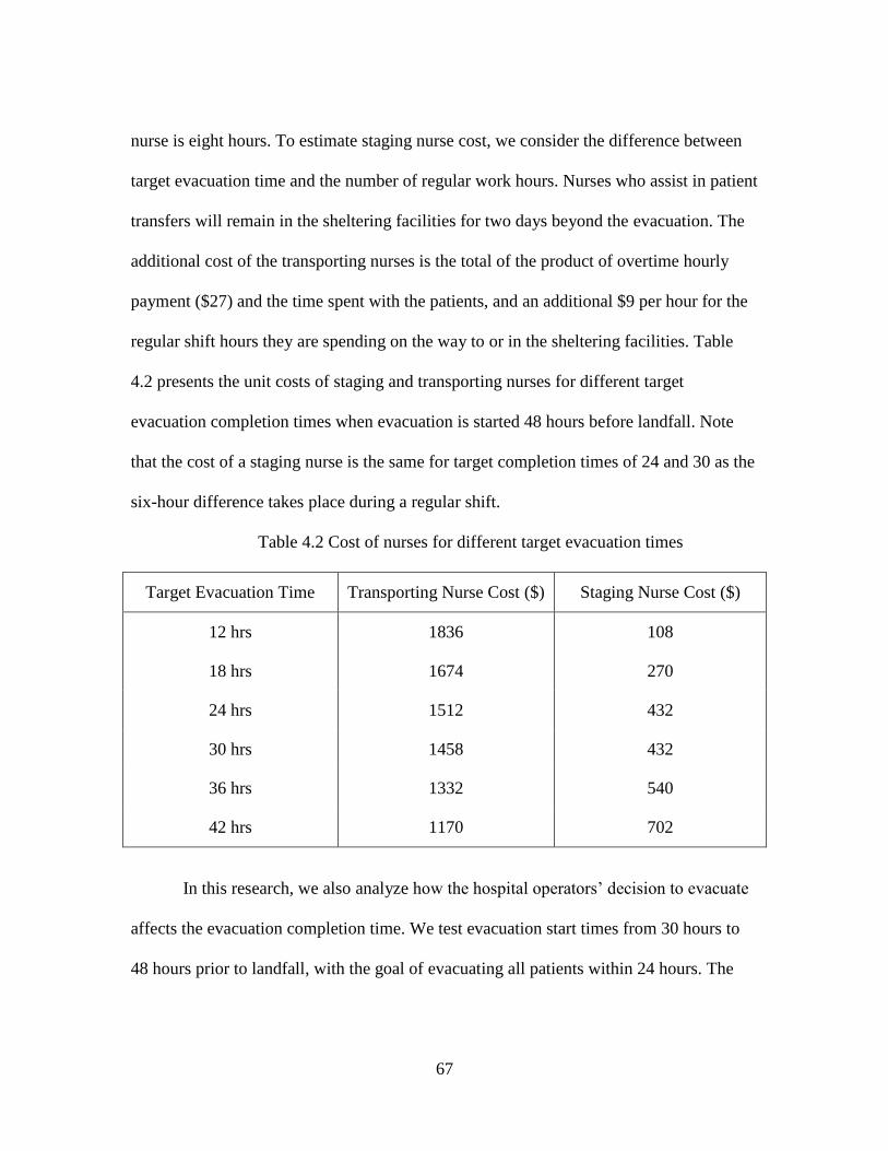
67

nurse is eight hours. To estimate staging nurse cost, we consider the difference between

target evacuation time and the number of regular work hours. Nurses who assist in patient

transfers will remain in the sheltering facilities for two days beyond the evacuation. The

additional cost of the transporting nurses is the total of the product of overtime hourly

payment ($27) and the time spent with the patients, and an additional $9 per hour for the

regular shift hours they are spending on the way to or in the sheltering facilities. Table

4.2 presents the unit costs of staging and transporting nurses for different target

evacuation completion times when evacuation is started 48 hours before landfall. Note

that the cost of a staging nurse is the same for target completion times of 24 and 30 as the

six-hour difference takes place during a regular shift.

Table 4.2 Cost of nurses for different target evacuation times

Target Evacuation Time Transporting Nurse Cost ($) Staging Nurse Cost ($)

12 hrs 1836 108

18 hrs 1674 270

24 hrs 1512 432

30 hrs 1458 432

36 hrs 1332 540

42 hrs 1170 702

In this research, we also analyze how the hospital operators’ decision to evacuate

affects the evacuation completion time. We test evacuation start times from 30 hours to

48 hours prior to landfall, with the goal of evacuating all patients within 24 hours. The

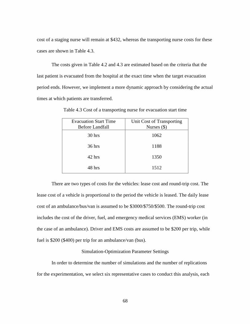
68

cost of a staging nurse will remain at $432, whereas the transporting nurse costs for these

cases are shown in Table 4.3.

The costs given in Table 4.2 and 4.3 are estimated based on the criteria that the

last patient is evacuated from the hospital at the exact time when the target evacuation

period ends. However, we implement a more dynamic approach by considering the actual

times at which patients are transferred.

Table 4.3 Cost of a transporting nurse for evacuation start time

Evacuation Start Time

Before Landfall

Unit Cost of Transporting

Nurses ($)

30 hrs 1062

36 hrs 1188

42 hrs 1350

48 hrs 1512

There are two types of costs for the vehicles: lease cost and round-trip cost. The

lease cost of a vehicle is proportional to the period the vehicle is leased. The daily lease

cost of an ambulance/bus/van is assumed to be $3000/$750/$500. The round-trip cost

includes the cost of the driver, fuel, and emergency medical services (EMS) worker (in

the case of an ambulance). Driver and EMS costs are assumed to be $200 per trip, while

fuel is $200 ($400) per trip for an ambulance/van (bus).

Simulation-Optimization Parameter Settings

In order to determine the number of simulations and the number of replications

for the experimentation, we select six representative cases to conduct this analysis, each

69

case having three sheltering facilities with 40/80/40 bed capacities for Type 1/2/3

patients. We also assume the evacuation begins 48 hours before landfall and all patients

are aimed to be evacuated within 24 hours.

Allocations of resources are obtained for these cases with OptQuest, using cost

minimization as the objective. Automatic stop (Auto Stop) is selected as the terminating

condition for the optimization. Auto Stop implies that OptQuest stops automatically when

there has been no significant improvement in the best solution value after 100

simulations. In our tests, this usually turned out to be between 250 and 300 simulations.

Using the average total evacuation time as the performance measure, we run all

cases for 5 replications in order to find the half-width of the performance measure (see

Table 4.4). As seen, the range for the half-widths on patient time in system varies

between 0.25 hours (15 min) and 0.38 hours (22.8 min).

Table 4.4 Half widths of time in system performance measure

Transfer patients per type

[20,40,20] [40,80,40] [60,120,60] [80,160,80] [100,200,100] [120,240,120]

Half-width

(in hours) 0.36 0.34 0.33 0.38 0.25 0.32

We choose to find the number of replications that reduces the half-width to less

than 0.17 hours (or 10 minutes) for all cases. The number of replications found by both

approximation formulas, explained previously, to obtain the desired half-width value for

all cases is displayed in Table 4.5. Clearly, approximation 1 results in a higher replication

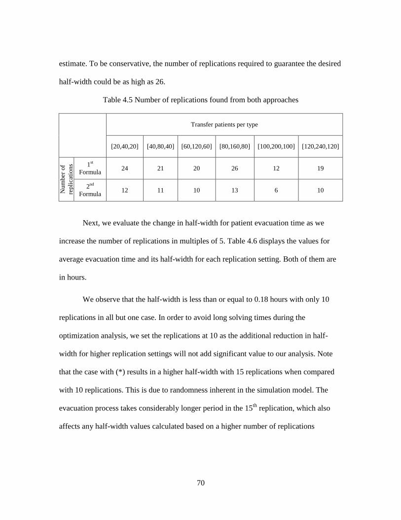
70

estimate. To be conservative, the number of replications required to guarantee the desired

half-width could be as high as 26.

Table 4.5 Number of replications found from both approaches

Transfer patients per type

[20,40,20] [40,80,40] [60,120,60] [80,160,80] [100,200,100] [120,240,120]

Nu

mb

er o

f

rep

lica

tio

ns 1

st

Formula 24 21 20 26 12 19

2nd

Formula 12 11 10 13 6 10

Next, we evaluate the change in half-width for patient evacuation time as we

increase the number of replications in multiples of 5. Table 4.6 displays the values for

average evacuation time and its half-width for each replication setting. Both of them are

in hours.

We observe that the half-width is less than or equal to 0.18 hours with only 10

replications in all but one case. In order to avoid long solving times during the

optimization analysis, we set the replications at 10 as the additional reduction in half-

width for higher replication settings will not add significant value to our analysis. Note

that the case with (*) results in a higher half-width with 15 replications when compared

with 10 replications. This is due to randomness inherent in the simulation model. The

evacuation process takes considerably longer period in the 15th

replication, which also

affects any half-width values calculated based on a higher number of replications

71

Table 4.6 Analysis for number of replications

Number

of

replications

Transfer patients per type

[20,40,20] [40,80,40] [60,120,60] [80,160,80]* [100,200,100] [120,240,120]

Total

Time

Half-

width

Total

Time

Half-

width

Total

Time

Half-

width

Total

Time

Half-

width

Total

Time

Half-

width

Total

Time

Half-

width

5 18.88 0.36 18.87 0.34 21.78 0.33 22.75 0.38 22.24 0.25 22.68 0.32

10 18.85 0.17 18.92 0.15 21.90 0.17 22.83 0.22 22.20 0.11 22.77 0.18

15 18.84 0.13 18.91 0.11 21.86 0.13 23.14 0.42 22.21 0.12 22.71 0.13

20 18.87 0.11 18.90 0.09 21.87 0.10 22.99 0.33 22.20 0.11 22.70 0.12

25 18.85 0.09 18.89 0.08 21.89 0.08 23.07 0.32 22.20 0.09 22.73 0.10

30 18.83 0.09 18.88 0.08 21.89 0.08 23.06 0.27 22.20 0.08 22.74 0.09

In parallel, we investigate the effect of the number of simulations to run during

the simulation-optimization analysis. Both replications and simulations have similar

effects in sharpening the answer that OptQuest will produce, however increasing either of

these measures adds computation time. Therefore, while testing for the number of

simulations to run, we reset the replication setting to 5. The same six cases are run with

different termination rules: Auto Stop, 500, 750, and 1000 simulations (See Appendix 5

for detailed information). Table 4.7 displays the evacuation cost, as well as total and

relative improvement from the Auto Stop option when we increase the number of

simulations. It is seen that the improvement from Auto Stop ranges from 0.01% to 4.03%.

However, most of the improvement is gained by setting the number of simulations at 500.

72

Table 4.7 Analysis for number of simulations

Transfer

patients per

type

Number of

Simulations

Evacuation

Cost

Best

Simulation No

Improvement

from Auto

Stop (%)

Relative

Improvement

(%)

[20, 40, 20]

Auto Stop 90849 241 N/A N/A

500 90843.6 469 0.01 0.01

750 90843.6 469 0.01 0.00

1000 90843.6 469 0.01 0.00

[40, 80, 40]

Auto Stop 178708.20 263 N/A N/A

500 174859.40 486 2.20 2.20

750 174639.00 520 2.33 0.13

1000 174639.00 520 2.33 0.00

[60, 120, 60]

Auto Stop 269382.2 256 N/A N/A

500 260399 451 3.45 3.45

750 260399 451 3.45 0.00

1000 258934.6 955 4.03 0.57

[80, 160, 80]

Auto Stop 346976.2 184 N/A N/A

500 342115.4 332 1.42 1.42

750 339759.4 740 2.12 0.69

1000 338298.6 935 2.57 0.43

[100, 200, 100]

Auto Stop 432930.4 270 N/A N/A

500 432224 486 0.16 0.16

750 431468 524 0.34 0.18

1000 431468 524 0.34 0.00

[120, 240, 120]

Auto Stop 523547.4 257 N/A N/A

500 512017.8 452 2.25 2.25

750 512017.8 452 2.25 0.00

1000 509726 978 2.71 0.45

At this setting, the relative improvements were much larger than the improvements

observed with either 750 or 1000 simulations. Obtaining results with 500 simulations and

10 replications takes about approximately two hours, which implies there is a trade-off

73

between time and the result values. Considering that each scenario tested by OptQuest

will require this time, we chose to find a parameter setting that would require no more

than one hour of solving time per case. To reduce solving time approximately in half, we

should either choose 5 replications with 500 simulations or 10 replications with Auto

Stop (250-300 simulations). The half-width of the performance measure ranges from 0.32

hr (19 min) to 0.38 hr (23 min) when the number of replication is used as 5. Since most

of the evacuation test cases require several hours for the evacuation to be completed, a

slight change in half-width beyond 10 minutes will not have a detrimental effect on the

system. However, having 500 simulations instead of what typically resulted from Auto

Stop (250-300 simulations) improves the solutions considerably. Thus, we choose to use

5 replications with 500 simulations during the optimization analysis.

Sensitivity Analysis

Effects of Different Target Evacuation Times

Cost Structure 1

One of the key outcomes from this research is the fact that we can provide

hospital operators with resource requirements that have been tested over many scenarios.

In addition, we now have the ability to perform many sensitivity analyses. We begin by

considering the effects of different target evacuation times on the allocation of resources.

We analyzed all previously defined cases; selecting one case (for both 3 and 15 shelter

options) for presentation, we record results for target evacuation window increases from

12 hours to 42 hours (see Appendix 6). Table 4.8 presents the critical statistics regarding

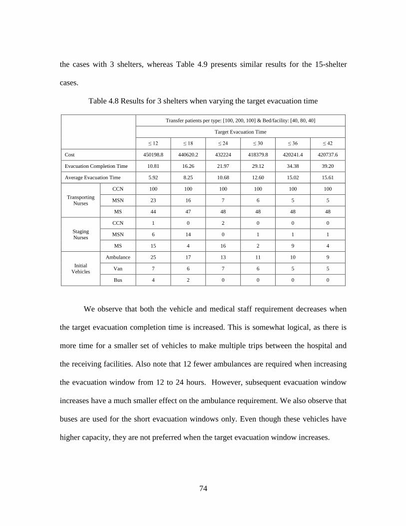
74

the cases with 3 shelters, whereas Table 4.9 presents similar results for the 15-shelter

cases.

Table 4.8 Results for 3 shelters when varying the target evacuation time

Transfer patients per type: [100, 200, 100] & Bed/facility: [40, 80, 40]

Target Evacuation Time

≤ 12 ≤ 18 ≤ 24 ≤ 30 ≤ 36 ≤ 42

Cost 450198.8 440620.2 432224 418379.8 420241.4 420737.6

Evacuation Completion Time 10.81 16.26 21.97 29.12 34.38 39.20

Average Evacuation Time 5.92 8.25 10.68 12.60 15.02 15.61

Transporting

Nurses

CCN 100 100 100 100 100 100

MSN 23 16 7 6 5 5

MS 44 47 48 48 48 48

Staging

Nurses

CCN 1 0 2 0 0 0

MSN 6 14 0 1 1 1

MS 15 4 16 2 9 4

Initial Vehicles

Ambulance 25 17 13 11 10 9

Van 7 6 7 6 5 5

Bus 4 2 0 0 0 0

We observe that both the vehicle and medical staff requirement decreases when

the target evacuation completion time is increased. This is somewhat logical, as there is

more time for a smaller set of vehicles to make multiple trips between the hospital and

the receiving facilities. Also note that 12 fewer ambulances are required when increasing

the evacuation window from 12 to 24 hours. However, subsequent evacuation window

increases have a much smaller effect on the ambulance requirement. We also observe that

buses are used for the short evacuation windows only. Even though these vehicles have

higher capacity, they are not preferred when the target evacuation window increases.

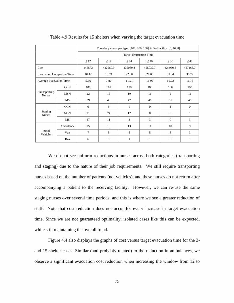
75

Table 4.9 Results for 15 shelters when varying the target evacuation time

Transfer patients per type: [100, 200, 100] & Bed/facility: [8, 16, 8]

Target Evacuation Time

≤ 12 ≤ 18 ≤ 24 ≤ 30 ≤ 36 ≤ 42

Cost 445572 442569.9 435080.8 425032.7 424960.8 427163.7

Evacuation Completion Time 10.42 15.74 22.80 29.06 33.54 38.79

Average Evacuation Time 5.56 7.80 11.21 11.96 15.03 16.78

Transporting Nurses

CCN 100 100 100 100 100 100

MSN 22 18 10 11 5 11

MS 39 40 47 46 51 46

Staging Nurses

CCN 0 5 0 0 1 0

MSN 21 24 12 0 6 1

MS 17 11 3 3 0 3

Initial

Vehicles

Ambulance 25 18 13 11 10 9

Van 7 5 5 5 5 3

Bus 6 3 1 1 0 1

We do not see uniform reductions in nurses across both categories (transporting

and staging) due to the nature of their job requirements. We still require transporting

nurses based on the number of patients (not vehicles), and these nurses do not return after

accompanying a patient to the receiving facility. However, we can re-use the same

staging nurses over several time periods, and this is where we see a greater reduction of

staff. Note that cost reduction does not occur for every increase in target evacuation

time. Since we are not guaranteed optimality, isolated cases like this can be expected,

while still maintaining the overall trend.

Figure 4.4 also displays the graphs of cost versus target evacuation time for the 3-

and 15-shelter cases. Similar (and probably related) to the reduction in ambulances, we

observe a significant evacuation cost reduction when increasing the window from 12 to

76

30 hours. We actually see a slight increase in cost for subsequent periods, which may

simply mean that eventually the cost of having staff on evacuation pay rates for a long

time will begin to outweigh other factors. With the exception of the 12-hour window, it

is slightly more expensive to operate with 15 sheltering facilities as opposed to 3.

Figure 4.4 Cost values of base case versus target evacuation time

Cost Structure 2

As there are expected to be many alternate cost structures in place across all

hospitals, we consider a second set of costs—one in which the relative costs of the

evacuation process do not change over time. This assumes that there is an agreement

about fixed costs between the hospital and its staff as well as the vehicle leasing

companies. Moreover, medical staff would likely begin another rotation at their regular

pay, so we could have a fixed evacuation cost per nurse. We define the alternate cost

structure as follows. The cost of a staging nurse is $500, and if a staging nurse becomes a

transporting nurse later, s/he is paid an extra $1500. The lease costs of the

77

ambulance/bus/van are $3000/$750/$500, respectively. Vehicle round-trip costs are the

same as before. The model is run for the same cases by inserting these new cost

parameters into the simulation-optimization model (see Appendix 7). Figure 4.5 displays

the resulting evacuation costs against target evacuation completion time.

Figure 4.5 Cost values of alternate case versus target evacuation time

We again observe cost reductions as the target evacuation completion time

increases, where extending the evacuation window beyond 36 hours does not have a

significant impact.

Effects of Different Evacuation Start Times

There is always discussion among hospital operators of beginning their

evacuation prior to the community-wide evacuation. By avoiding traffic congestion at

peak evacuation times, patients could be transferred more quickly (and safely) to shelter

facilities. We investigate how the initial start time of the hospital evacuation affects the

overall completion time.

78

Cost Structure 1

Table 4.10 and 4.11 present the critical statistics for the same representative cases

with 3 and 15 shelters as in the previous section, where we now run simulations for

evacuation start times between 30 to 48 hours prior to landfall (see Appendix 8). All

patients are to be evacuated within 24hours.

Table 4.10 Results for 3 shelters when varying the evacuation start time

Transfer patients per type: [100, 200, 100] & Bed/facility: [40, 80, 40]

Evacuation Start Before Landfall

30 36 42 48

Cost 378628 399985 414135 426759.2

Evacuation Completion Time 23.96 23.35 20.54 22.6

Average Evacuation Time 11.99 10.52 9.00 10.9

Transporting Nurses

CCN 100 100 100 100

MSN 13 13 9 7

MS 48 46 46 49

Staging Nurses

CCN 1 1 0 0

MSN 0 8 6 4

MS 1 3 8 0

Initial Vehicles

Ambulance 17 17 15 13

Van 8 7 9 7

Bus 1 1 0 0

By beginning the evacuation earlier, there are fewer ambulances necessary due to

reduced roadway congestion. We also notice substantial increases in evacuation cost as

the hospital evacuation is initiated earlier. While the evacuation completion time is not

increasing, the transporting nurses are required for up to 18 more hours across the start

time options in the tables. Each nurse will continue to be paid at the evacuation rate

during this time.

79

Table 4.11 Results for 15 shelters when varying the evacuation start time

Transfer patients per type: [100, 200, 100]

Evacuation Start Before Landfall

30 36 42 48

Cost 380552 400882.4 414682.6 435297.6

Evacuation Completion Time 23.54 22.17 21.80 22.18

Average Evacuation Time 12.31 9.62 10.40 9.84

Transporting

Nurses

CCN 100 100 100 100

MSN 19 20 12 8

MS 43 40 46 50

Staging Nurses

CCN 1 0 0 0

MSN 1 7 0 0

MS 7 9 6 9

Initial Vehicles

Ambulance 17 17 15 13

Van 4 5 6 8

Bus 3 3 1 0

We illustrate this comparison of cost against evacuation start time in Figure 4.6.

Comparing the two cases, it is seen that it costs slightly more to evacuate patients to 15

shelters than to 3 shelters.

Figure 4.6 Cost values of base case versus evacuation start times

80

Cost Structure 2

Using the alternate set of system costs, we run a similar analysis by varying

evacuation start time. Figure 4.7 displays the resulting cost values versus evacuation

completion times for these cases (see Appendix 9 for detailed results). The cost values, in

general, decrease as the start time of evacuation before landfall is extended. We also see

that it costs more if patients are evacuated to 15 shelters instead of 3 shelters.

Figure 4.7 Cost values of alternate case versus evacuation start times

While cost can be a major consideration in evacuation planning (especially in

situations where federal reimbursement funding is in question), we ultimately are

concerned with how quickly we can get patients out of harm’s way. To address this, we

evaluate the influence of the evacuation start time on the evacuation completion time.

The same six cases as described in the section of simulation-optimization parameter

settings are used in this analysis. In order to provide a consistent comparison for all

evacuation start times, we fix the set of resources for each of the six cases. To find the

81

base set of resources, we used simulation-optimization with a target evacuation

completion time of 24 hours and an evacuation start time of 36 hours before landfall. We

then assumed that the hospital operator could choose to evacuate between 24 and 60

hours before landfall (see Table 4.12).

Table 4.12 Influence of evacuation start time on evacuation completion time

Time

between

evacuation

start and

landfall

Evacuation Completion Time

Transfer patients per type

[20,40,20] [40,80,40] [60,120,60] [80,160,80] [100,200,100] [120,240,120]

24 (*) -- -- -- -- -- --

30 20.42 23.29 23.65 23.71 23.63 23.98

36 16.14 22.00 22.08 23.29 23.17 23.64

42 13.81 17.10 17.26 17.91 17.79 18.72

48 13.01 15.95 15.99 16.50 13.12 17.16

54 13.01 15.67 15.74 16.16 12.94 16.83

60 13.01 15.67 15.74 16.16 12.94 16.83

(*) Note that evacuation completion time is not given when evacuation start time is 24

hours before landfall as some patients cannot be evacuated.

It is seen that some of patients cannot be evacuated when evacuation start time is

24 hours before landfall, whereas all of the patients can be evacuated for the other

evacuation start times. The evacuation completion time increases as the evacuation start

time before landfall decreases. When evacuation start time is 30 hours before landfall, the

82

evacuation completion time is very close to 24 hours, which is very risky in terms of

evacuating patients as evacuation process stops six hours before landfall. Note that the

cases with evacuation start times of 54 and 60 hours before landfall have same evacuation

completion time because there is unabated traffic flow at that time.

Although having an early evacuation start time seems to be the best, the hospital

operators should take into account the costs regarding evacuation and select the best

evacuation start time for their facility.

Concluding Remarks

There exist many probabilistic events inherent in the evacuation process of

hospitals in case of a hurricane event. We propose a simulation model that takes into

account these stochastic events. The simulation model is built as general and flexible as

possible in order to allow all risk managers to test evacuation plans by only entering

some input data parameters. By embedding this simulation model into an optimization

model, the vehicle and nurse requirements can be presented with the objectives of

minimizing cost within a pre-specified evacuation completion time. This research

investigates the effects of target evacuation completion time and the effects of the

decisions made by the hospital operators regarding the evacuation start time on the

allocation of resources.

One major limitation of the proposed methodology is that the deviation from

optimality cannot be evaluated due to not having a lower bound model. Note that the

lower bound model in Chapter 3, LP relaxation of [HEM] cannot be used to obtain

83

optimality gaps as the methodology in Chapter 4 includes many stochastic events, which

differentiate both methodologies significantly and prevents the use of the lower bound

model used in Chapter 3. Another limitation is that it does not include the real-time

traffic, which affects the allocation of the resources, as the traffic factor included into the

simulation model is assumed. Main drawback of simulation modeling is building it based

on the specified rules. As the rules change, the simulation modeling needs to be modified.

In this research, we consider one traffic policy and one set of rules for the allocation of

the resources. For evaluating different traffic policies and sets of rules regarding the

allocation of the resources, additional effort is required to modify the simulation model.

84

CHAPTER FIVE

RESOURCE ALLOCATION AND CUSTOMER SELECTION FOR PERIODIC

DELIVERY AND DISTRIBUTION PROBLEM

Introduction

While in Chapter 3 and 4, our objective is to identify optimal (or near optimal)

resource assignments to support an evacuation operation in a limited timeframe (e.g., 1-2

days), we now consider how to manage production and customer selection decisions

when the operation requires periodic deliveries. Recall that the focus of this dissertation

is to find resource requirements and schedules for various logistics operations, and we

will illustrate how the constructs within our Chapter 3 model formulation apply directly

to the product delivery and distribution problem.

There are many cases where the companies and their subcontractor companies

tend to build their production facilities close to each other or the companies select the

subcontractors from nearby region so that subcontractors can make frequent deliveries in

order to reduce the inventory costs. These subcontractor companies may receive more

order than they are able to satisfy due to the restrictions on their budget and space.

Therefore, they need to select a subset of customers among their customer base while

making tactical decisions. Within the context of operational decisions, they also need to

find out the resource requirements for the production and distribution processes to meet

the orders of the selected customers.

85

In this research, we only focus on finding the requirements and schedules of the

resources for the logistics operations as it was our interest throughout this dissertation.

When literature is reviewed in the area of delivery and distribution systems, it is seen that

researchers focused on finding routing schedules and inventory policies, but did not aim

to solve the resource requirements problem. This research addresses the resource

requirements problem for the delivery and distribution systems and contributes

methodologies to solve this problem while meeting all orders of the customers or

selecting the most profitable set of customers. We propose a new product delivery and

distribution model that presents the allocation and schedules of the resources required to

deliver the orders of all customers within a pre-specified period of time with the objective

of maximizing profit. With minor additions and modifications to this product delivery

and distribution model, we propose two new models that select customers according to

all-or-nothing principle with the storage and budget restrictions, respectively. These two

models not only present the customers to support, but also present the allocation and

schedules of the resources for the logistics operations. Similar to Chapter 3, all test

instances cannot reach to optimality with the proposed models. Therefore, heuristics,

which are similar in structure to those in Chapter 3, are proposed for all models.

Methodology

System Overview

Consider a subcontractor firm for which tactical and operational decisions are

evaluated. This firm produces a variety of products to meet a set of customer orders at the

86

firm’s facility. Each customer has unique demand for each type of product and generate

unique amount of revenue for each type of product. Same as the case with every supply-

chain system, the firm has restrictions on the budget, thereby on the number of resources,

and storage space.

The firm has a long-term contract with a logistics company to deliver the products

from the production facility to the facilities of the customers. The logistics company only

provides the vehicles, trucks in this case, and the drivers. The firm has flexibility in types

of the vehicles, as well as the time periods in which deliveries are made to its customer

base. It is assumed that there is no restriction on the number of vehicles that are rented

and the number of drivers. The drivers are only responsible for driving the vehicles, and

not responsible for loading the products onto the vehicles and unloading them in the

customers’ facilities. At the end of the day, the drivers park the vehicles in the

subcontractor firms’ parking spot if they will be used by the firm the next day. The firm

and the customers need to hire hourly employees to handle the loading/unloading of the

products.

The number of product i loaded onto the vehicle depends on the volume of the

product and the size of the truck, while the number of product i a material handler can

load depends only on the volume of the product. Multiple products can be transported on

the same vehicle.

During each delivery, a vehicle goes to only one customer and returns back for

the next deliveries. It is assumed that customers are all approximately one period t away

87

from the firm, which means that all trips require one period t and the process of

loading/unloading the products is assumed to be done within one period t.

As mentioned earlier, this research focus on the plans regarding delivery and

distribution processes and presents a novel approach to find the required number of the

vehicles and material handlers and the schedules of the vehicle trips in the aim of

maximizing profit. It also presents which customers to select when they cannot meet all

of the customer orders due to storage and budget restrictions.

Delivery and Distribution Model

In this section, the proposed model, which presents the allocations and schedules

of the resources for the delivery processes to meet all of the customer orders while

maximizing profit, is given in detail. All time-dependent events are assumed to be

deterministic.

This model evaluates the operating plans of the firm that produces I product types

and has a potential pool of J customers. The logistics company gives the firm an option

of selecting vehicles out of K vehicle types. The delivery processes need to be completed

within T hours.

The notations and definitions of the parameters defined in this optimization model

are given below:

ijd : Customer j demand for product i

v

ikr : Percentage of capacity used when one unit of product i is transported in a type k

vehicle

88

D

i: Percentage of a material handler used while loading one unit of product i onto a

vehicle

p

ic : Cost of procuring/producing one unit of product i

v

kc : Cost of one round-trip of a type k vehicle

d

sc : Cost of material handlers per shift

v

kf : Lease cost of a type k vehicle for time period T

ijr : Per-unit revenue of product i

The notations and definitions of the decision variables defined in this model are

given below:

Yijkt : Amount of product i loaded for shipment to customer j in a type k vehicle in

period t

Vkt : Number of type k vehicles ready to deliver product during period t

vjkt : Number of type k vehicles delivering product to customer j during period t

max

sN : Total material handler requirement

The delivery and distribution model (DDM) can now be presented as:

[DDM] Maximize

1 1 1 1

I J K Tp

ij i

i j k t

r cmax

0

1 1 1 1 1

J K T K Sv v d

ijkt k jkt k k s s

j k t k s

Y c v f V c N

(1)

Subject to

Vehicle Locations: ( 1)

1

J

kt k t jkt

j

V V v k = 1,…,K, t = 1,2,3,4, (2)

89

( 1) ( 4)

1 1

J J

kt k t jkt jk t

j j

V V v v k = 1,…,K, t = 5,…,T, (3)

0kT kV V k = 1,…,K, (4)

Demand Allocated: 1 1

K T

ijkt ij

k t

Y d i = 1,…,I, j = 1,…,J, (5)

Vehicle Assignments: ( 1)

1

Iv

ik ijkt jk t

i

r Y v j = 1,…,J,k = 1,…,K, t = 1,…,T, (6)

M..Handler Requirements: max

1 1 1

I J KD

i ijkt s

i j k

Y N i = 1,…,I, j = 1,…,J,s=1,t = 1,…,8, (7)

max

1 1 1

I J KD

i ijkt s

i j k

Y N i = 1,…,I, j = 1,…,J,s=2,t = 9,…,T, (8)

Integrality: max, , 0jkt ijkt sv Y N and integer i = 1,…,I , j = 1,…,J,k = 1,…K,

s=1,..,S,t = 1,…,T+1, (9)

Nonnegativity: 0ktV i = 1,…,I, j = 1,…,J,t = 1,…,T. (10)

As mentioned earlier, the loading/unloading of products and traveling between the

production facility and customers are assumed to each take one period t. Therefore, it

takes three periods between the departure and return of the vehicles. In order to deliver

the products in the specified period T, we do not allow the start of delivery from the

production facility after period T-3 by adding the set of constraints below:

0ijktY i = 1,…,I , j = 1,…,J, k = 1,…K, t = T-2,..,T. (11)

In essence, we have a model somewhat similar in structure to the one in Chapter

3. The mapping of the similar decision variables and data parameters of the models

[HEM] and [DDM] is presented with their notations in Table 5.1.

90

Table 5.1 Mapping of decision variables and data parameters

[HEM] [DDM]

Decision

variables

ijktY ijktY

ktV ktV

jktv jktv

s

tN max

sN

Data

parameters

v

ikr v

ikr

s

ir D

i

v

kc v

kc

2

nc d

sc

v

kf v

kf

As seen in Table 5.1, notations of the mapping decision variables and data

parameters are mostly same in [HEM] and [DDM]. Also, the constraint sets (2), (3), (6),

(8) of [HEM] map to the constraint sets (2), (3), (6), and (7 & 8) of [DDM]. Due to the

differences in the logistic operations of the systems, there are unique constraints, which

require additional data parameters, in both of the models. [HEM] also have more decision

variables due to the systems’ resource requirement for accompanying with the patients

and staying with them in sheltering facilities.

This model considers a profit objective while finding the allocations and

schedules of the resources to satisfy customer orders. The profit is calculated as the

difference between sales revenue of the products and total cost of the production and

distribution. The total cost of the production and distribution is the sum of the total

procurement/production cost, the total round-trip cost of vehicle, the total lease cost of

the vehicles, and the total cost of the material handlers.

91

The constraint sets (2) and (3) update the number of available vehicles at the

production facility in period t. As it takes four periods to deliver a set of goods to a

customer, there are only vehicles that leave the production facility for t=1,2,3,4, and

vehicles start to return during period t=5. The constraint set (4) implies that all vehicles

must return back and be at the facility at the end of the period T, while the constraint set

(5) enforces to meet all customer orders. The constraint set (6) restricts the amount of

product i loaded for shipment to customer j in a type k vehicle during period t to the

capacity of Type k vehicles that goes to customer j in the next period.

In experimentation, we evaluate operating plans of this firm for 16 hours, T, and

assume that there exist two shifts, each of which is 8 hours. Similar to the constraint set

(6) the constraint set (7) restricts the amount of product i loaded for shipment to

customer j in a type k vehicle during period t to the number of material handlers required

in the first shift, while the constraint set (8) restricts that to the required material handlers

in the second shift. In a case which has more than two shifts, additional constraint sets

similar to the constraint sets (7) and (8) needs to be added, whereas constraint set (8) can

be eliminated if there is only one shift. If a shift is not 8 hours, then the range of t in these

constraints should be modified according to the time ranges each shift take place.

Solution Approach to [DDM]

Exact Solution

We test the proposed optimization model [DDM] with a large number of test

instances via a commercial solver, ILOG OPL Development Studio 5.2 which uses ILOG

CPLEX as the engine. The computers that are used during these test analysis have Core 2

92

Duo CPUs @ 2.33 GHz with 2 GB of RAM. It is seen that some of these test instances

can reach to optimality with [DDM] due to the program memory limitations. In addition

to solving some of the test instances to optimality, we notice variability in the solving

times. This leads to the investigation of alternate methods for consistently obtaining

solutions to this problem.

Identifying an Upper Bound Model

[DDM] cannot reach the optimal solution for most of the test instances due to

memory limitation issues. We follow the same approach as in Chapter 3 and firstly

investigate how to obtain a quality upper bound quickly and consistently. Certain

integrality restrictions are relaxed, and the following key measures are taken into

consideration while selecting the best upper bound: 1) guarantee of upper bound, 2) upper

bound quality, and 3) solving time.

The linear programming (LP) relaxation is selected as one of the alternative upper

bound models as it relaxes all integer restrictions and gives the highest bound to the

objective. While deciding on the alternative upper bound models, the strategy of relaxing

an integrality restriction at a time is employed. Thus, three alternative upper bound

models given below are considered first:

1. LP Relaxation

2. Integrality restrictions except the one for jktv variables are relaxed.

3. Integrality restrictions except the one for ijktY variables are relaxed.

The alternative upper bound model with the integrality restrictions except the one

for max

sN is not into consideration as max

sN is a decision variable array with only one index

93

and does not have significant effect on the long solving times and memory usage of the

computer.

Same test instances used in the previous section are tested with these alternative

lower bound models. These models are compared according to their ability to guarantee

solution, provide quick solving times, and achieve a high bound quality, where bound

quality (or gap) is calculated using those test cases for which optimal solutions could be

found. Alternative 1 and 3 can solve all the test instances in less than a second with the

same bound quality, 2.07%, whereas Alternative 2 cannot solve most of the test

instances. As Alternative 3 can solve all the test instances in less than a second, we

considered one more alternative upper bound model, Alternative 4, in which only jktv

variables are relaxed. The aim for considering this alternative is to reduce the relaxation

gap by having an alternative upper bound model as close to MILP as possible. At the end

of this investigation, Alternative 4 is selected as the best alternative upper bound model

because of its capability in solving all the cases in less than a second with the lowest

relaxation gap, 1.83%.

Heuristic Studies

Fractional assignments of vehicles are obtained with Alternative 4. Therefore, a

heuristic is needed to identify a feasible solution to [DDM], which should be as close to

the unknown optimal solution as possible. We proposed a two-step heuristic, Heuristic

[DDM], the steps of which are presented below:

1. Run Alternative 4 of [DDM].

2. Run MILP of [DDM], in which all ijktY decision variables are set to the ijktY

94

values obtained in Step 1.

This heuristic can be considered as a good solution approach to [DDM] in spite of

the deviation from optimality as it obtains solution for all test instances in a considerably

short period of time with a sizable gap

Customer Selection Model with Limited Resource Availability

In the previous section, we propose a solution approach to find the allocations and

schedules of the resources for the delivery processes when the firm does not have any

restrictions on budget, storage space, etc. However, every company has some level of

restrictions on its resources and most of them have a large customer base, all orders of

which they cannot satisfy due to these restrictions. Therefore, they need to select the set

of customers that will maximize their profit.

In this research, we propose a new model for the capacitated systems that selects a

set of customers according to the all-or-nothing principle. According to this principle, if

the firm selects a customer, it has to meet all orders of that customer. This model is

obtained by making minor additions and modifications to [DDM]. The constraint set (4)

in [DDM] is modified as follows:

1 1

K T

ijkt ij

k t

Y d i = 1,…,I, j = 1,…,J,

The constraint set (4) is equality in [DDM] for enforcing the model to meet all

customer orders. As the firm will not meet some of the customers’ orders, 1 1

K T

ijkt

k t

Y is

allowed to be zero and restricted to be at most ijd for that particular i and j by making this

constraint set inequality.

95

For this model, a binary variable array with one index, zj, defined as follows:

0 if customer is not selected

1 if customer is selectedj

jz

j

Besides, a new constraint is added to ensure that all orders of the customer are

satisfied if selected.

1 1 1 1

I K T I

ijkt ij j

i k t i

Y d z j = 1,…,J,

We refer to this model as customer selection/delivery and distribution model,

abbreviated as [CSDDM]. In the next sections, we introduce two possible resource

restrictions, storage space and budget, respectively. According to the restriction type, a

restriction constraint needs to be added to [CSDDM], which will be presented in those

sections.

As mentioned earlier, [CSDDM] not only presents the set of the customers with

maximum profit, but also finds out the allocations and schedules of the resources utilized

during the delivery processes.

[CSDDM] with Storage Capacity Restriction

Most of the companies have limited storage space used for keeping the raw

materials, work-in-process inventory and finished goods before delivery. In this section,

we investigate the effects of the limitations of the storage space, used only for finished

goods before delivery, on the selection of customers.

In order to do this, we add a restriction constraint for storage space to [CSDDM]

as shown:

96

1 1 1 1

*(1 )I J K T

i ijkt Heuristic

i j k t

m Y Unit volume

, where mi = per-unit volume of product i

Unit-volume Heuristic = total unit-volume requirement to meet all of the customer

orders found with the use of heuristic method

= percentage of restriction on the total unit-volume requirement.

This constraint restricts the amount of product i loaded for shipment to customer j

in a type k vehicle during period t to the unit-volume available in the firms’ facility. We

refer to this model as restricted storage customer selection/delivery and distribution

model and abbreviate as [RSCSDDM].

We tested [RSCSDDM] with the same test instances used in previous section for

two different levels of storage restrictions via the commercial solver. Similar to [HEM]

and [DDM], some of the test instances can result in optimal solution with [RSCSDDM]

due to the program memory limitations and it also takes long time to solve some of the

solvable test instances. Therefore, the same approach used in the previous section, two-

step heuristic, is utilized again. However, the heuristic is modified slightly as the models

are different. Below are the steps of the heuristic, Heuristic [RSCSDDM]:

1. Run Alternative 4 of [RSCSDDM]

2. Run MILP of [RSCSDDM], in which all ijktY decision variables are set to the

ijktY

values obtained in Step 1.

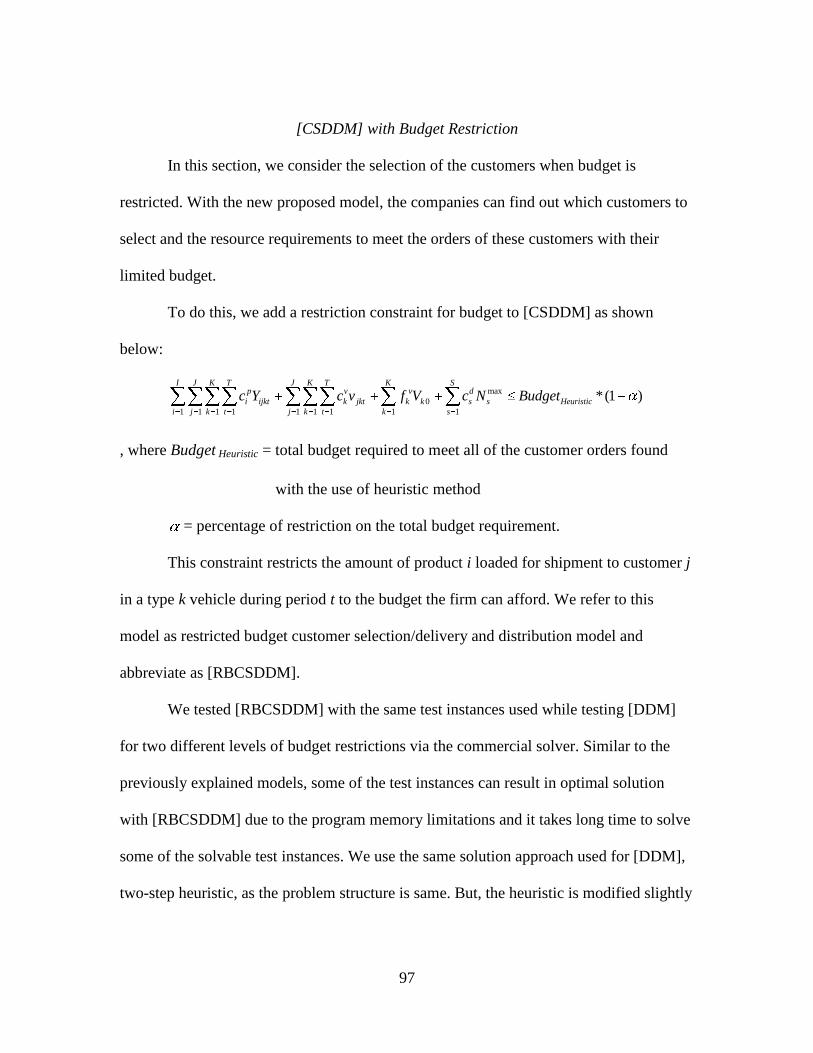
97

[CSDDM] with Budget Restriction

In this section, we consider the selection of the customers when budget is

restricted. With the new proposed model, the companies can find out which customers to

select and the resource requirements to meet the orders of these customers with their

limited budget.

To do this, we add a restriction constraint for budget to [CSDDM] as shown

below:

max

0

1 1 1 1 1 1 1 1 1

*(1 )I J K T J K T K S

p v v d

i ijkt k jkt k k s s Heuristic

i j k t j k t k s

c Y c v f V c N Budget

, where Budget Heuristic = total budget required to meet all of the customer orders found

with the use of heuristic method

= percentage of restriction on the total budget requirement.

This constraint restricts the amount of product i loaded for shipment to customer j

in a type k vehicle during period t to the budget the firm can afford. We refer to this

model as restricted budget customer selection/delivery and distribution model and

abbreviate as [RBCSDDM].

We tested [RBCSDDM] with the same test instances used while testing [DDM]

for two different levels of budget restrictions via the commercial solver. Similar to the

previously explained models, some of the test instances can result in optimal solution

with [RBCSDDM] due to the program memory limitations and it takes long time to solve

some of the solvable test instances. We use the same solution approach used for [DDM],

two-step heuristic, as the problem structure is same. But, the heuristic is modified slightly

98

as the model has additional constraints and variables. Below are the steps of the heuristic,

Heuristic [RBCSDDM]:

1. Run Alternative 4 of [RBCSDDM]

2. Run MILP of [DDM], in which all ijktY decision variables are set to the ijktY

values obtained in Step 1.

In the second step of this heuristic; we use MILP of [DDM] as we intend to relax

the budget restriction. Otherwise, infeasible solutions can be obtained for some test

instances as the solution found by Alternative 4 of [RBCSDDM] can be tight in the

budget restriction constraint and when we eliminate the fractional assignment of vehicles,

the budget may increase and pass the budget limitation. Therefore, the firm should

calculate the budget for the resulted allocation of resources or it should consider

allowance with the consideration of the associated costs of the vehicles while finding the

allocation of resources with the use of this heuristic.

Experimentation

Parameter and Test Settings

We determine a set of parameter and test settings to evaluate the proposed model.

In this section, parameter settings and test settings used for the experimentation will be

explained in detail, respectively.

The firm can produce two different product types (I=2): Product 1 and Product 2.

The proportion of the volume of Product 1 to Product 2 1 2[ / ]m m is 2. The logistics

company gives two options for the vehicle types (K=2), which we refer as Type 1/2 truck

99

throughout this chapter, with a volume proportion of 2/3, respectively. 100/200

(11 21[1/ ] / [1/ ]r r ) Product 1/2 can be located on a Type 1 truck at a time, while 150/300

(12 22[1/ ] / [1/ ]r r ) Product 1/2 can be located on a Type 2 truck at a time. A material

handler can load 75/150 (1/ s

i ) Product 1/2 onto any type of vehicle in a period t.

A period is assumed to be an hour in length. As mentioned in the previous

section, we are evaluating the daily distribution plans of the firm and it is assumed that

there exist two shifts (S) in a day, each of which takes 8 hours. Thus, T is assigned as 16.

The unit production cost of a Product 1/2 is $200/140 ( 1 2/p pc c ), while unit

revenue for each order set of Product 1/2 is drawn from uniform distribution, which will

be referred as U hereafter, and the distributions are U [$220, $260] / U [$160, $200]

( 1 2/j jr r ) for each customer, respectively. The daily lease cost of a Type 1/2 truck is

$400/$600 ( 1 2/v vf f ), respectively, while the round-trip cost of a Type 1/2 truck is

$290/$390 ( 1 2/v vc c ), respectively, which is the total of the cost of the gas price and the

driver. The hourly cost of a material handler is $30, which makes the cost of a material

handler per shift as $240 ( 1

dc ). However, a material handler working in the second shift

should be considered as working for 5 hours because products are not allowed to be

loaded onto the vehicle in the last 3 hours so as to deliver the products to the customers in

16 hours, which makes the cost of a material handler that works in the second shift as

$150 ( 2

dc ).

During experimentation, we consider two different delivery types: single-product

delivery and two-product delivery. For the single-product delivery, we test the model for

100

both of the products, Product 1 and Product 2. Also, we test two different demand

distributions ( 1 jd ), DD1 and DD2, to observe the effect of demand on the allocation of

resources:

DD1: abbreviation used instead of U [200, 400]

DD2: abbreviation used instead of U [400, 600]

For the two-product delivery, we consider two approaches for the demand. In the

first approach, both of the products are demanded according to the same distribution,

DD1 or DD2, whereas each one is demanded from different distributions, DD1 or DD2,

in the second approach. Within the context of second approach, we consider two different

sub-cases, MDD1 and MDD2:

MDD1: the case when the demand distribution of Product 1/2 ( 1 2/j jd d ) is U

[200, 400] / U [400, 600], respectively.

MDD2: the case when the demand distribution of Product 1/2 ( 1 2/j jd d ) is U

[400, 600] / U [200, 400], respectively.

In addition, we consider five different levels for the number of customers (J): 3, 5,

10, 15, and 20. Also, we generate 20 test instances for each case. To sum up, a total of

800 test instances are used for experimentation.

Solutions of [DDM]

Exact Solution Results

These cases are tested to optimality with the proposed model [DDM] via

commercial solver. However, only 98 out of 800 test instances resulted in optimal

solutions due to program memory limitations.

101

Table 5.2 presents all of the cases in which an optimal solution was obtained with

[DDM]. This table displays the profit, budget, required unit-volume, and allocation of

vehicles and material handlers obtained as a result of the optimization runs of these cases.

Note that some of the test instances of these cases can not result in optimal solution.

Therefore, the result values in Table 5.2 are the average of the optimally solvable test

instances.

Table 5.2 Cases resulting in optimal solutions with the [DDM]

Delivery Type

Single Product Two-

Product

(SDD*) Product Type 1 Product Type 2

Number of

customers 3 3 5 3

Demand

distribution DD1 DD2 DD1 DD2 DD1 DD1

Profit 30745 52317.5 32653.5 55153 53187.82 66014.67

Budget 184908 301353.33 128999.5 214217.5 206995.45 313429.33

Unit-volume 1800 2942.83 900 1500 1447.73 2690.93

Veh

icle

Type 1 1.7 0.83 1.5 0.45 1.64 1.27

Type 2 1.3 3.17 0.5 1.95 1.18 2.6

Mat

eria

l

Han

dle

r 1st Shift 2 2 1.85 2 2 2

2nd

Shift 1.7 2 0.8 1.15 1 2

Solving Time 1944.54 1377.96 28.41 192.13 4347.54 3257.35

(*) SDD is the abbreviation for same demand distribution.

When the cases are compared according to their demand distributions and

delivery types, it is seen that the allocation of Type 1 truck decreases, while the allocation

of Type 2 truck increases as demand increases because the model opts for allocating more

102

trucks with more volume capacity due to the increase in demand. Also, as demand

increases, the requirement for material handlers slightly increases, whereas profit, budget

and unit-volume requirement increases considerably. Besides, it is seen that the

requirement of material handlers for the 2nd

shift is mostly less than or equal to the

requirement of material handlers for the 1st. When the cases with different number of

customers, 3 and 5, are compared, it is seen that there exist slightly difference in the

allocation of vehicles and material handlers, while having approximately proportional

increase in the profit, budget, and required unit-volume.

As mentioned before, most of the cases cannot be solved to optimality. Also, it is

seen that it may take considerably long time to solve a test instance to optimality. This

motivates the investigation of alternate methods for obtaining solutions to the delivery

and distribution problem.

Heuristic Results

All of the test instances, 800, are solved with Heuristic [DDM] in less than a

second. In order to evaluate the performance of Heuristic [DDM], we computed the

integrality and optimality gaps for each case. The gap between the solutions of MILP and

heuristic, referred to as integrality gap, is calculated as follows:

100MILP Heuristic

Heuristic

Objective ObjectiveIntegrality Gap

Objective

The average integrality gaps of the cases for which optimal solutions can be

obtained are presented in Table 5.3.

103

Table 5.3 Integrality Gaps

Delivery

Type

Single Product Two

Product

(SDD) Product 1 Product 2

Number of

customers 3 3 5 3

Demand

distribution DD1 DD2 DD1 DD2 DD1 DD1

Integrality

gap 12.85 4.51 15.25 9.48 12.31 5.73

The gap between the solutions of LP relaxation and heuristic, referred to as

optimality gap, is computed as follows:

100LP Heuristic

Heuristic

Objective ObjectiveOptimality Gap

Objective

The average optimality gaps of all cases are presented in Table 5.4. When Table

5.3 and 5.4 are analyzed, it is seen that the gaps decrease when more products are

delivered.

Table 5.4 Optimality Gaps

1 Product Type 2 Product Types

Product 1 Product 2 Same Demand

Distributions

Different Demand

Distributions

Demand

distribution DD1 DD2 DD1 DD2 DD1 DD2 MDD1 MDD2

Nu

mb

er o

f C

ust

om

ers

3 16.26 5.74 18.94 11.31 6.66 5.89 5.93 6.52

5 8.65 5.36 13.89 4.39 7.11 3.84 4.80 4.35

10 6.99 4.20 6.52 3.90 5.19 2.63 3.48 4.02

15 6.29 3.25 6.15 2.89 4.40 2.35 3.15 3.14

20 5.05 2.66 5.06 2.69 3.77 1.93 2.60 2.77

104

This can be observed by comparing the cases with different number of customers,

different demand distributions and different production types. This is due to the fact that

the effect of the cost of the vehicles on the profit decreases when the revenues and

production costs increase due to the increase in demand. Also, when integrality gaps and

optimality gaps are compared, it is observed that the gaps are very close to each other.

Thus, the solution of MILP is closer to the solution of LP relaxation than it is to the

solution of heuristic.

Table 5.5 presents the averages of profit, budget, required unit-volume, and

allocations of vehicles and material handlers resulted from the proposed heuristic for

Product 1 and Product 2 when the firm serves to three customers in a single-product

delivery system. Recall that these averages are obtained from 20 test instances. Also,

summary result values obtained from the heuristic for all the cases are tabulated in

Appendix 10.

When Table 5.5 and tables in Appendix 10 are analyzed, it is seen that profit,

budget, required unit-volume, allocation of vehicles and material handlers increase as

demand increases. When the results obtained from MILP and heuristic are compared, it is

observed that the firm mostly needs to allocate only Type 2 trucks according to the

heuristic results whereas the firm needs to allocate both of the truck types according to

MILP results. This is due to the fact that 1ij tY values are mostly obtained as zero with the

alternative upper bound model, Alternative 4, which is used in the first step of the

heuristic, due to relaxation of the integrality restriction on jktv . As we examine the tables

105

in Appendix 10, it is also seen that the allocations of material handlers in 1st and 2

nd shifts

are almost same.

Table 5.5 Sample Results Obtained from Heuristic [DDM]

Product Type Product 1 Product 2

Demand distribution DD1 DD2 DD1 DD2

Profit 27566.5 49989.5 28609 50646.5

Budget 188086.5 309403.5 133044 218746.5

Unit-volume 1800 3000 900 1500

Vehicle

Type 1 0 0 0 0

Type 2 4.9 5.65 4.2 5.55

Material

Handler

1st Shift 1.5 2.05 1 1

2nd

Shift 1.75 2.1 1 1.1

Sensitivity Analysis

Two graphs in Figure 5.1 and Figure 5.2 are presented to observe the effect of the

number of customers on profit and budget, respectively, in more detail. In both figures,

the graphs on the left-side are obtained from the cases with DD1 as demand distribution,

whereas the graphs on the right-side are obtained with DD2 as demand distribution.

As explained earlier and seen in Figure 5.1, the profit increases proportionally

when demand increases due to increase in number of customers and/or number of product

106

Figure 5.1 Profit analyses with same demand distribution

Figure 5.2 Budget analyses with same demand distributions

types delivered. Similarly, budget increases proportionally when demand increases (see

Figure 5.2). When the profits of delivering Product 1 and 2 in a single-product delivery

system are compared, it is seen that the profit of Product 2 is slightly higher than that of

Product 1. On the other hand, it is observed that the budget of Product 1 is considerably

107

higher than that of Product 2. Recall that Product 1 occupies double space of Product 2.

Thus, it can be concluded that Product 2 should be preferred in a single-product delivery

system if demand rates are enough for the firm to work with full capacity as it results in

higher profit with smaller budget and less storage space requirement.

Figure 5.3 displays the same analysis for the two-product delivery type with

different demand distributions. In Figure 5.3, the graph on the left-hand side presents the

profit versus number of customers, whereas the graph on the right-side displays the

budget versus number of customers. It is seen that the cases with MDD1 results in

slightly higher profit, except the case with 5 customers, while requiring less budget when

compared to the cases with MDD2. Thus, it can be concluded that the firm can gain more

profit with less investment when there is more demand to Product 2.

Figure 5.3 Profit and budget analyses for two-product delivery type with different

demand distributions

108

Solutions of [RSCSDDM]

For testing [RSCSDDM], we consider two levels of storage restriction: 25% and

50%. These two levels of restrictions are applied to 800 test instances used in the

previous section. Thus, a total of 1600 test instances are tested in the experimentations

associated with [RSCSDDM].

Exact Solution Results

All test instances are tested with the proposed model [RSCSDDM] via the

commercial solver. Only 563 out of 1600 test instances resulted in optimal solutions due

to program memory limitations. When we compared the optimality analysis of [DDM]

and [RSCSDDM], it is seen that we obtain optimal solutions to more test instances with

[RSCSDDM]. Although the model is expected to be harder to solve, more test instances

can be solved to optimality in shorter period of time as the solution can be found more

easily due to the reduction in solution space.

All of the test instances with 3 customers, some of the test instances with 5

customers, and a few of the test instances with 10 customers can be solved to optimality,

whereas none of the test instances with 15 and 20 customers can be solved to optimality.

Appendix 11 presents the tables of the average result values obtained from all of the

optimally solvable test instances. In addition to the result values presented in similar

tables, these tables present the average number of selected customers.

Table 5.6 presents the optimal result values for the case, which has a customer

base of 3 to deliver Product 1 in a single-product delivery system, obtained with [DDM]

and [RSCSDDM].

109

Table 5.6 A few cases resulting in optimal solutions with [DDM] and [RSCSDDM]

Demand

Distribution DD1 DD2

Storage restriction 0% 25% 50% 0% 25% 50%

Unit-volume 1800 1181.9 665.3 2942.83 1999.9 1052.8

Number of

selected customers 3 1.95 1.05 3 2 1

Profit 30745 22354.35 13805.05 52317.5 38536.7 22295.4

Budget 184908 121662 68818 301353.33 205118 108425

Vehicle

Type 1 1.7 1.2 0.45 0.83 1.75 0.85

Type 2 1.3 0.8 0.75 3.17 1.25 1.05

Material

Handler

1st Shift 2 2 1.9 2 2 2

2nd

Shift 1.7 1.7 0.75 2 2 0.55

When the restriction on the storage space increases, profit, budget, unit-volume

requirement, and the allocation of vehicles reduce at a higher rate than the proportional

rate. Besides, it is seen that there is no trend in the allocation of each truck type when the

storage space restriction increases. Additionally, the allocation of material handlers does

not change when storage space is restricted by 25%, while the allocation of material

handlers, especially in the 2nd

shift, decreases when restriction increases from 25% to

50%.

Heuristic Results

Heuristic [RSCSDDM] is used to solve all test instances (see Appendix 12). It is

worth mentioning that the heuristic could not solve 12 test instances of the cases with 3

customers and 1 test instance of the case with 5 customers while we obtain optimal

110

solutions for the same test instances in less than a minute. As optimal solution can be

obtained for those test instances in less than a minute, no further investigation is done to

improve Heuristic [RSCSCCM].

As mentioned previously, all of the test instances with 3 customers can be solved

with the optimization model [RSCSDDM]. It takes less than a second to solve most of the

test instances; however the maximum solving time of all the test instances with 3

customers is 2271.91 sec. Therefore, it is suggested to solve the test instances with 3

customers by using [RSCSDDM] if time is allowed. Otherwise, heuristic can be used to

solve the test instances.

Table 5.7 presents the result values of the cases same as in Table 5.6 obtained

with the use of heuristic. Similarly, profit, budget, and required unit-volume reduce at a

higher rate than the proportional rate when the level of storage space restriction increases.

The allocation of material handlers among different storage space is specific to a case it

stays same or it reduces as less storage space is allowed. The allocation of Type 2 truck

reduces when less storage space is allowed, while the firm does not need to allocate any

Type 1 truck. Same as the situation with [DDM], 1ij tY values are mostly obtained as zero

with the alternative upper bound model, Alternative 4, which is used in the first step of

the heuristic, due to relaxation of the integrality restriction on jktv . Although this results in

some sizable relaxation gaps for the cases with small number of customers, the gaps

reduce significantly as problem size increases when the number of customer increases

and/or when more than one product is delivered. The integrality and optimality gaps for

all the cases are given in Appendix 13.

111

Table 5.7 – Sample Results Obtained from Heuristic [RSCSDDM]

Sensitivity Analysis

To analyze the effects of storage space restriction on profit, two graphs of the case

with 10 customers in single-product delivery and two-product delivery with same

demand distributions are presented in Figure 5.4. The graph on the left-hand side

presents the profit versus storage space restriction level for the cases with DD1, whereas

the graph on the right-hand side presents that for the cases with DD2. It is seen that the

decreasing rate is steeper for the cases with higher demand. This can be seen when the

graphs on left-hand side and right-hand side are compared, and when the cases with two-

product delivery are compared. Also, the case with only Product 2 delivery is slightly

Demand Distribution DD1 DD2

Storage restriction 25% 50% 25% 50%

Unit-volume 1199.33 663.6 2000.89 1052.8

Number of

selected customers 1.94 1.07 2 1

Profit 19743.39 11275.8 38316.06 19591.9

Budget 126513.33 70882 207205.56 111070

Vehicle

Type 1 0 0 0 0

Type 2 3.89 2.47 3.89 3.15

Material

Handler

1st Shift 1 1 2 1

2nd

Shift 1 1 2 1

112

more profitable than the case with only Product 1 delivery even when the storage space is

restricted.

Figure 5.4 Profit analyses with same demand distributions when space is restricted

Figure 5.5 displays a similar analysis for the two-product delivery with different

demand distributions with the same case used in Figure 5.4.

Figure 5.5 Profit analyses for two-product delivery type with different demand

distributions when space is restricted

113

When Figure 5.5 is analyzed, it is seen that there is slightly difference between

two cases in terms of profit. Also, it is observed that the difference between the profits of

the two cases decreases as the storage space is more restricted.

Solutions of [RBCSDDM]

Similar to storage restriction analysis, we consider two levels of budget

restriction, 25% and 50%, for the experimentation. These two levels of restrictions are

applied to 800 test instances used for [DDM]. Thus, a total of 1600 test instances are

tested in the experimentations associated with [RBCSDDM].

Exact Solution Results

All test instances are tested to optimality with the proposed model [RBCSDDM]

via the commercial solver. Only 524 out of 1600 test instances resulted in optimal

solutions due to program memory limitations. Same as the case with the storage

restriction, it is seen that we obtain optimal solutions to more test instances with

[RBCSDDM] than [DDM]. Although the opposite case is expected, the test instances can

be solved with [RBCSDDM] more easily than [DDM] as the solution space is narrowed

down.

Similar to [RSCSDDM], all of the test instances with 3 customers, some of the

test instances with 5 customers, and a few of the test instances with 10 customers can be

solved to optimality, whereas none of the test instances with 15 and 20 customers can be

solved to optimality. Appendix 14 presents the tables of the average result values

obtained from all of the optimally solvable test instances.

114

Table 5.8 presents the optimal result values for the case, which has a customer

base of 3 to deliver Product 1 in a single-product delivery system, obtained with [DDM]

and [RBCSDDM]. When the restriction on the budget increases, profit, budget, unit-

volume requirement, and the allocation of vehicles reduce at a higher rate than the

proportional rate. Besides, it is seen that there is no trend in the allocation of each truck

type, the total material handler requirement, and the material handler requirement in each

shift when the level of budget restriction increases.

Table 5.8 A few cases resulting in optimal solutions with [DDM] and [RBCSDDM]

Demand

Distribution DD1 DD2

Budget restriction 0% 25% 50% 0% 25% 50%

Budget 188086.5 121662 68818 309403.5 207548 108366.5

Number of

selected customers 3 1.95 1.05 3 2 1

Profit 27566.5 22354.35 13805.5 49989.5 39206.35 22295.4

Unit-volume 1800 1181.9 665.3 3000 2023.7 1052.8

Vehicle

Type 1 0 1.20 0.45 0 1.65 0.85

Type 2 4.9 0.80 0.75 5.65 1.35 1.05

Material

Handler

1st

Shift 1.5 2.00 1.9 2.05 2 2.00

2nd

Shift 1.75 1.70 0.75 2.1 2 0.55

Heuristic Results

Heuristic [RBCSDDM] is used to solve all test instances (see Appendix 15).

Similar to the situation with [RSCSDDM], we encounter the same condition of not being

able to solve a few test instances with heuristic, while solving them to optimality in

115

considerably short period of time. No further study is done in order to improve Heuristic

[RBCSDDM] as those test instances can be solved to optimality in considerably short

period of time.

Same as the case with [RSCSDDM], it is seen that all of the test instances with 3

customers can be solved with [RBCSDDM]. It takes less than a second to solve most of

the test instances; however the maximum solving time of all the test instances with 3

customers is 2208.88 sec. Therefore, it is suggested to solve the test instances with 3

customers by using [RSCSDDM] if time is allowed. Otherwise, heuristic can be used to

solve these test instances.

When heuristic results are analyzed, same observations are made: profit, budget,

and required unit-volume reduce at a higher rate than the proportional rate when the level

of budget restrictions is made; and the allocation of Type 1 trucks are almost zero due to

same reason explained earlier. The integrality and optimality gaps for all the cases are

given in Appendix 16. Note that integrality gaps are found with MILPs, which have

budget restriction constraint, whereas the optimality gaps are found with LPs, which also

have budget restriction constraint, while the second step of the heuristic does take into

account the budget restriction in order to prevent infeasibility. Therefore, it is not a fair

evaluation for the gaps, but they are given in order to present an approximation of how

close our heuristic to the optimal solution.

Last but not least, we investigate the level of exceeding the allowed budget as the

second step of Heuristic [RBCSDDM] enables to pass beyond the allowed budget. Table

5.9 presents the averages of the percentage of difference in budget obtained in 1st and 2

nd

116

steps of the heuristic, number of solutions exceeding the allowed budget, the percentage

of exceeding the allowed budget, and maximum percentage of exceeding the allowed

budget.

Table 5.9 Feasibility analysis for budget

Number of Customers

3 5 10 15 20

Percentage of difference

in budget 2.06 1.8 1.33 1.08 0.98

Number of solutions

exceeding the budget 0.02 0.09 0.39 0.44 0.71

Percentage of exceeding

the allowed budget 0.03 0.14 0.37 0.34 0.53

Maximum of percentages

of exceeding the allowed

budge

4.63 4.31 3.69 1.83 1.88

It is seen that the level of exceeding budget increases slightly as the problem size

increases due to the number of customers. The maximum of percentages of exceeding the

allowed budget among all customer levels is 4.63%. Thus, he firm should consider 5% of

allowance for its target budget while making decisions about their budgets. As mentioned

earlier, this allowance depends on the system parameters and the firm should calculate

the budget for the resulted allocation of resources or it should consider some allowance

by taking account the associated costs of the resources before making this kind of

analysis.

117

Concluding Remarks

In this section, we apply the same techniques used in Chapter 3 for a periodic

delivery and distribution problem. First of all, a deterministic optimization model is

proposed that present the allocation of resources required for delivery processes to meet

all orders of the customers while maximizing profit. A total of 800 test instances are

tested to optimality. However, the model is unable to solve most of the test instances due

to memory limitations. Therefore, a two-step heuristic is proposed, which solves all test

instances less than a second with acceptable relaxation gaps.

Next, we consider two possible restrictions on the resources of companies for

meeting all orders of the customers: storage space and budget. We propose two new

models that select customers and find the resource requirements for delivery processes

for the firms with limited storage space and budget. Similarly, only some of the test

instances can be solved to optimality, which requires us to use the same heuristic

approaches. Finally, we solve all 800 test instances for two different levels of restrictions,

25% and 50%, with the use of heuristic method and investigate the results in detail.

Similar to Chapter 3, one of the limitations of the proposed methodologies is that

a constant transport time of one period is assumed for all customers. Loading and

unloading of the products is assumed to require one period each. Another major

limitation is that all time-dependent events are assumed to be deterministic. In addition,

the methodologies results in feasible solutions, not optimal, with some sizable gaps.

118

CHAPTER SIX

CONCLUSIONS AND RECOMMENDATIONS

Conclusions

In this research, we focused on the allocation and scheduling of resources for the

logistics operations. We investigate two different two different types of logistics systems:

logistics system of the health care facilities during emergency evacuation and delivery

and distribution system of production industries. Although these systems seem very

different, they are mainly similar in terms of the structure of the operations and

differences of them are insignificant details.

Firstly, we investigate the logistic operations that take place during hospital

evacuation. When literature is reviewed, it is seen that there exists no research that

proposes a quantitative technique to solve the resource requirements and scheduling

problem for the emergency evacuations of the hospitals. This research fills this gap and

contributes a methodology to solve this problem. We propose a deterministic mixed

integer linear programming that enables the risk managers of the hospitals evaluate their

evacuation plans in case of an advanced notice event such as hurricane. This model also

presents the allocations and schedules of the vehicles and nurses required for evacuating

all of the patients within a pre-specified period of time while minimizing cost. With the

use of CPLEX and OPL 5.2, 36 cases are tested for the target evacuation completion time

ranging from 12 to 42. However, only 8 out of 36 cases can reach to optimality due to

memory limitations when the target evacuation time is 12 hours and it is seen that the

119

number of optimally solvable test instances decreases as the target evacuation time

increases and none of the cases can reach to optimality when the evacuation is aimed to

be completed within 42 hours due to the fact that it gets harder to solve the model

because of the increase in the complexity of the model as the number of constraints and

variables increases. To solve this problem, we firstly search for an alternate lower bound

by relaxing the integrality restrictions and select LP relaxation among four others as it is

the only one that can solve all of the cases in less than a second. Due to the fractional

solution resulting from LP, we propose a variable rounding heuristics based on LP

Relaxation to obtain feasible solutions for all of the cases. Also, we develop this heuristic

and suggest a rounding heuristic with local search, which provided very little

improvement over the initial heuristic. By means of this heuristic, we solve all the test

cases in considerably short period of time. Additionally, we investigate the assignments

of nurses and vehicles and the effects of different target evacuation times. Lastly, the

resource requirements and their schedules are found for another objective, minimizing

evacuation completion time, with a limited budget.

However, many of the events surrounding hospital evacuation are inherently

probabilistic and task durations are often uncertain. Therefore, we contribute another

methodology to solve the same problem while accounting for uncertainties in the

evacuation process. We also address the variability in transfer times by accounting

roadway congestion via a traffic factor. We propose a stochastic model via simulation to

evaluate the evacuation plans of the hospitals: stochastic model via simulation. It is seen

that hospitals have their unique steps to follow while evacuating the patients to the

120

sheltering facilities. We get information from many hospitals and developed a simulation

model based on most commonly used steps. The simulation is built as flexible as possible

so that any risk manager can test many scenarios for his/her hospital with minimum and

very simple inputs. We firstly investigate the parameter settings for the number of

simulations and number of replications to use in simulation-optimization analysis. Next,

we analyze the effects of different target evacuation times and different evacuation start

times before landfall on the allocation of resources. We also examine the effects of the

decisions regarding evacuation start time on evacuation completion time and the ability to

evacuate all of the patients.

Lastly, we apply the same techniques used in Chapter 3 for a periodic delivery and

distribution problem. Next, we propose a deterministic mixed integer linear

programming, which has the same structure as the model introduced in Chapter 3, to

present the allocation of resources required for delivery processes of a firm to meet all

orders of the customers while maximizing profit. We develop 40 cases with different

product types, different delivery types, and different demand levels and generate 20 test

instances for each case, which results in a total of 800 test instance. Similarly, we test all

of these test instances for optimality with the use of CPLEX and OPL 5.2. However, the

model is unable to solve all the test instances due to memory limitations. To solve all test

instances in considerably short period of time, we propose a two-step heuristic based on

alternate lower bound model. It solves all test instances less than a second with

acceptable relaxation gaps. It is seen that the relaxation gap decreases as the size of the

problem increases due to the increase in number of customers and/or number of products

121

delivered, which means that the effect of the cost of the vehicle on the objective

decreases when the system gets bigger. Then, we take into account the possible

limitations on the resources, storage space and budget, that prevents the firm to satisfy the

orders of all of the customers. With minor changes in the model proposed in this section,

we propose two new models that select the most profitable set of customers while

presenting the required resources for the delivery operations in a system with restricted

storage space/budget, respectively. We test two levels of restriction for each resource

type, which makes a total of 1600 test instances for each of the resource restrictions.

Then, we attempt to solve all of them to optimality and obtain optimal solution for some

of them. It is seen that more cases can result in optimal solution when the system is

restricted in terms of storage space or budget than when it is not restricted. Although the

opposite is expected, this may be a result of narrowing down the solution space with

these restrictions. As the models are slightly different, we propose tailored solution

approaches for these two models, which are slightly different than the proposed heuristic

for the model with no restriction.

Recommendations

The proposed methodologies for both of the systems have some limitations

mentioned in each section. To overcome these limitations, research can be done with the

purposes as listed below. In the context of logistic systems of health care facilities during

emergency evacuation:

To find better heuristics for solving [HEM]

122

To improve the methodology in Chapter 3 by allowing the time flexibility in terms

of the transport time to each sheltering facility, loading patients onto the vehicles,

and unloading patients in the sheltering facilities.

To build dynamic representation of the system where either the admissions or

releases of the patients are known in advance or stochastic changes are required to

be included to the facility census.

To find a lower bound model in order to compare the deviation from optimality

with the proposed simulation-optimization approach

To make suggestions for improving the polices related to the allocation of the

resources by creating alternative simulation models

To explore search algorithms that can be integrated with the proposed simulation

model

To integrate dynamic traffic assignment with the proposed simulation model and to

evaluate different traffic policies

In the context of delivery and distribution systems of the production industries:

To find better heuristics for solving [DDM], [RSCSDDM] and [RBCSDDM]

To improve the proposed methodologies by allowing the time flexibility in terms

of the transport time to the customers, and loading and unloading of the products

To find a methodology that allows the vehicles do multi-trips

To integrate the proposed methodologies with a proposed inventory routing

methodology in literature

To find methodology that consider stochastic nature of the environment

123

APPENDICES

124

Appendix 1

Optimization Result Tables

Results of Cases with 3 Shelters for the Target Evacuation Completion Time of 12 Hours

Transfer patients per type: [20, 40, 20] Transfer patients per type: [40, 80,40]

MILP LP H1 H2 MILP LP H1 H2

Cost 84570 82022.92 90633 88689

Out of

Memory

164045.83 169740 169740

Evacuation Time 12 12 12 12 12 12 12

Transport Nurses 30 29.17 32 31 58.33 60 60

Ambulance 7 6.67 7 7 13.33 14 14

Van 0 0 0 0 0 0 0

Bus 2 1.53 3 3 3.06 4 4

Solving Time 14.95 0.01 0.03 0.25 3333.04 0.01 0.03 0.28

Optimality Gap N/A N/A 10.50 8.13 N/A N/A 3.47 3.47

Transfer patients per type: [60, 120, 60] Transfer patients per type: [80, 160, 80]

MILP LP H1 H2 MILP LP H1 H2

Cost

Out of

Memory

246068.75 253410 253410*

Out of

Memory

328091.67 337980 335061

Evacuation Time 12 12 12 12 12 12

Transport Nurses 87.5 90 90 116.67 120 119

Ambulance 20 20 20 26.67 27 27

Van 0 0 0 0 0 0

Bus 4.58 6 6 6.11 8 7

Solving Time 21859.64 0.01 0.05 0.05 3298.33 0.01 0.03 0.24

Optimality Gap N/A N/A 2.98 2.98 N/A N/A 3.01 2.12

Transfer patients per type: [100, 200, 100] Transfer patients per type: [120, 240, 120]

MILP LP H1 H2 MILP LP H1 H2

Cost

Out of Memory

410114.58 419262 419262

Out of Memory

492137.5 498813 498813*

Evacuation Time 12 12 12 12 12 12

Transport Nurses 145.83 148 148 175 177 177

Ambulance 33.33 34 34 40 40 40

Van 0 0 0 0 0 0

Bus 7.64 10 10 9.17 11 11

Solving Time 2197.28 0.01 0.03 0.30 1286.54 0.01 0.03 0.03

Optimality Gap N/A N/A 2.23 2.23 N/A N/A 1.36 1.36

(*) No Available Swap

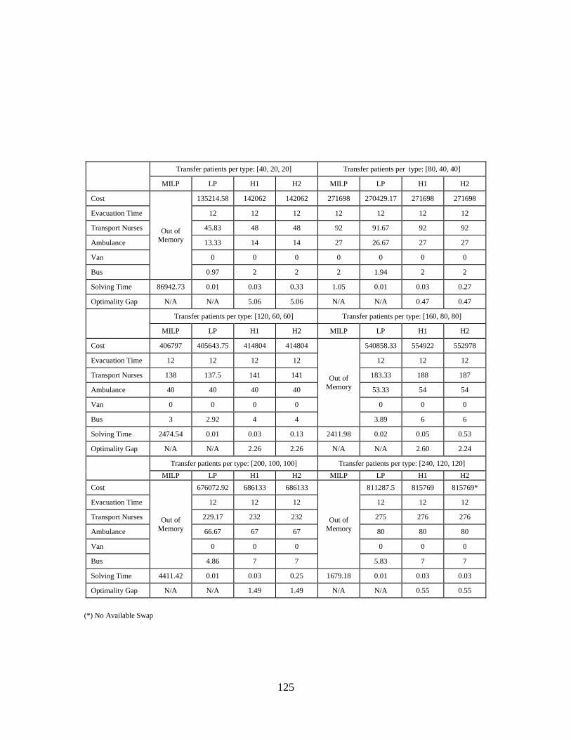
125

Transfer patients per type: [40, 20, 20] Transfer patients per type: [80, 40, 40]

MILP LP H1 H2 MILP LP H1 H2

Cost

Out of Memory

135214.58 142062 142062 271698 270429.17 271698 271698

Evacuation Time 12 12 12 12 12 12 12

Transport Nurses 45.83 48 48 92 91.67 92 92

Ambulance 13.33 14 14 27 26.67 27 27

Van 0 0 0 0 0 0 0

Bus 0.97 2 2 2 1.94 2 2

Solving Time 86942.73 0.01 0.03 0.33 1.05 0.01 0.03 0.27

Optimality Gap N/A N/A 5.06 5.06 N/A N/A 0.47 0.47

Transfer patients per type: [120, 60, 60] Transfer patients per type: [160, 80, 80]

MILP LP H1 H2 MILP LP H1 H2

Cost 406797 405643.75 414804 414804

Out of

Memory

540858.33 554922 552978

Evacuation Time 12 12 12 12 12 12 12

Transport Nurses 138 137.5 141 141 183.33 188 187

Ambulance 40 40 40 40 53.33 54 54

Van 0 0 0 0 0 0 0

Bus 3 2.92 4 4 3.89 6 6

Solving Time 2474.54 0.01 0.03 0.13 2411.98 0.02 0.05 0.53

Optimality Gap N/A N/A 2.26 2.26 N/A N/A 2.60 2.24

Transfer patients per type: [200, 100, 100] Transfer patients per type: [240, 120, 120]

MILP LP H1 H2 MILP LP H1 H2

Cost

Out of

Memory

676072.92 686133 686133

Out of

Memory

811287.5 815769 815769*

Evacuation Time 12 12 12 12 12 12

Transport Nurses 229.17 232 232 275 276 276

Ambulance 66.67 67 67 80 80 80

Van 0 0 0 0 0 0

Bus 4.86 7 7 5.83 7 7

Solving Time 4411.42 0.01 0.03 0.25 1679.18 0.01 0.03 0.03

Optimality Gap N/A N/A 1.49 1.49 N/A N/A 0.55 0.55

(*) No Available Swap

126

Transfer patients per type: [30, 30, 20] Transfer patients per type: [60, 60, 40]

MILP LP H1 H2 MILP LP H1 H2

Cost 110022 108618.75 113166 113166* 217600 217237.5 218325 218325*

Evacuation Time 12 12 12 12 12 12 12 12

Transport Nurses 38 37.5 39 39 75 75 75 75

Ambulance 10 10 10 10 20 20 20 20

Van 0 0 0 0 1 0 0 0

Bus 2 1.25 2 2 2 2.5 3 3

Solving Time 4.14 0.01 0.03 0.03 13.44 0.01 0.03 0.03

Optimality Gap N/A N/A 4.19 4.19 N/A N/A 0.5 0.5

Transfer patients per type: [90, 90, 60] Transfer patients per type: [120, 120, 80]

MILP LP H1 H2 MILP LP H1 H2

Cost

Out of

Memory

325856.25 330291 330291* 434475 434475 436650 436650*

Evacuation Time 12 12 12 12 12 12 12

Transport Nurses 112.5 114 114 150 150 150 150

Ambulance 30 30 30 40 40 40 40

Van 0 0 0 0 0 0 0

Bus 3.75 5 5 5 5 6 6

Solving Time 5580.94 0.01 0.03 0.03 0.09 0.01 0.03 0.03

Optimality Gap N/A N/A 1.36 1.36 N/A N/A 0.5 0.5

Transfer patients per type: [150, 150, 100] Transfer patients per type: [180, 180, 120]

MILP LP H1 H2 MILP LP H1 H2

Cost

Out of

Memory

543093.75 548616 548616*

Out of

Memory

651712.5 654975 654975*

Evacuation Time 12 12 12 12 12 12

Transport Nurses 187.5 189 189 225 225 225

Ambulance 50 50 50 60 60 60

Van 0 0 0 0 0 0

Bus 6.25 8 8 7.5 9 9

Solving Time 5558.20 0.02 0.05 0.05 3149.47 0.01 0.05 0.05

Optimality Gap N/A N/A 1.02 1.02 N/A N/A 0.5 0.5

(*) No Available Swap

127

Results of Cases with 15 Shelters for the Target Evacuation Completion Time of 12 hours

Transfer patients per type: [20, 40, 20] Transfer patients per type: [40, 80,40]

MILP LP H1 H2 MILP LP H1 H2

Cost

Out of

Memory

82022.92 92208 89289

Out of

Memory

164045.83 175434 175434

Evacuation Time 12 12 12 12 12 12

Transport Nurses 29.17 32 31 58.33 61 61

Ambulance 6.67 7 7 13.33 14 14

Van 0 0 0 0 0 0

Bus 1.53 4 3 3.06 6 6

Solving Time 20423.56 0.05 0.20 1.30 3215.13 0.05 0.20 1.23

Optimality Gap N/A N/A 12.42 8.86 N/A N/A 6.94 6.94

Transfer patients per type: [60, 120, 60] Transfer patients per type: [80, 160, 80]

MILP LP H1 H2 MILP LP H1 H2

Cost

Out of

Memory

246068.75 267480 267480*

Out of

Memory

328091.67 346449 346449

Evacuation Time 12 12 12 12 12 12

Transport Nurses 87.5 95 95 116.67 121 121

Ambulance 20 20 20 26.67 27 27

Van 0 0 0 0 0 0

Bus 4.58 8 8 6.11 11 11

Solving Time 5738.15 0.05 0.20 0.20 2966.53 0.03 0.19 1.22

Optimality Gap N/A N/A 8.7 8.7 N/A N/A 5.60 5.60

Transfer patients per type: [100, 200, 100] Transfer patients per type: [120, 240, 120]

MILP LP H1 H2 MILP LP H1 H2

Cost

Out of

Memory

410114.58 434538 434538

Out of

Memory

492137.5 516864 516864*

Evacuation Time 12 12 12 12 12 12

Transport Nurses 145.83 152 152 175 181 181

Ambulance 33.33 34 34 40 40 40

Van 0 0 0 0 0 0

Bus 7.64 14 14 9.17 16 16

Solving Time 1605.38 0.05 0.20 1.63 1364.11 0.06 0.22 0.22

Optimality Gap N/A N/A 5.96 5.96 N/A N/A 5.04 5.04

(*) No Available Swap

128

Transfer patients per type: [40, 20, 20] Transfer patients per type: [80, 40, 40]

MILP LP H1 H2 MILP LP H1 H2

Cost

Out of

Memory

135214.58 146556 146556

Out of

Memory

270429.17 284799 284799

Evacuation Time 12 12 12 12 12 12

Transport

Nurses 45.83 49 49 91.67 96 96

Ambulance 13.33 14 14 26.67 27 27

Van 0 0 0 0 0 0

Bus 0.97 4 4 1.94 5 5

Solving Time 2950.19 0.03 0.19 1.59 3022.57 0.05 0.20 1.31

Optimality Gap N/A N/A 8.39 8.39 N/A N/A 5.31 5.31

Transfer patients per type: [120, 60, 60] Transfer patients per type: [160, 80, 80]

MILP LP H1 H2 MILP LP H1 H2

Cost

Out of Memory

405643.75 423042 423042*

Out of Memory

540858.33 563529 563529

Evacuation Time 12 12 12 12 12 12

Transport

Nurses 137.5 143 143 183.33 191 191

Ambulance 40 40 40 53.33 54 54

Van 0 0 0 0 0 0

Bus 2.92 6 6 3.89 7 7

Solving Time 5463.71 0.05 0.20 0.20 3048.22 0.05 0.20 1.20

Optimality Gap N/A N/A 4.29 4.29 N/A N/A 4.19 4.19

Transfer patients per type: [200, 100, 100] Transfer patients per type: [240, 120, 120]

MILP LP H1 H2 MILP LP H1 H2

Cost

Out of

Memory

676072.92 704097 704097

Out of

Memory

811287.5 842709 842709

Evacuation Time 12 12 12 12 12 12

Transport

Nurses 229.17 238 238 275 286 286

Ambulance 66.67 67 67 80 80 80

Van 0 0 0 0 0 0

Bus 4.86 11 11 5.83 11 11

Solving Time 4158.89 0.05 0.20 1.86 1456.50 0.06 0.22 0.55

Optimality Gap N/A N/A 4.15 4.15 N/A N/A 3.87 3.87

(*) No Available Swap

129

Transfer patients per type: [30, 30, 20] Transfer patients per type: [60, 60, 40]

MILP LP H1 H2 MILP LP H1 H2

Cost 110022 108618.75 117060 117060*

Out of

Memory

217237.5 219300 219300*

Evacuation Time 12 12 12 12 12 12 12

Transport Nurses 38 37.5 40 40 75 75 75

Ambulance 10 10 40 40 20 20 20

Van 0 0 0 0 0 0 0

Bus 2 1.25 4 4 2.5 4 4

Solving Time 13465.12 0.03 0.20 0.20 4748.86 0.03 0.19 0.19

Optimality Gap N/A N/A 7.77 7.77 N/A N/A 0.95 0.95

Transfer patients per type: [90, 90, 60] Transfer patients per type: [120, 120, 80]

MILP LP H1 H2 MILP LP H1 H2

Cost

Out of

Memory

325856.25 335385 335385* 434475 434475 439800 439800*

Evacuation Time 12 12 12 12 12 12 12

Transport Nurses 112.5 115 115 150 150 150 150

Ambulance 30 30 30 40 40 40 40

Van 0 0 0 0 0 0 0

Bus 3.75 7 7 5 5 8 8

Solving Time 3663.40 0.05 0.20 0.20 1.38 0.05 0.23 0.23

Optimality Gap N/A N/A 2.92 2.92 N/A N/A 1.23 1.23

Transfer patients per type: [150, 150, 100] Transfer patients per type: [180, 180, 120]

MILP LP H1 H2 MILP LP H1 H2

Cost

Out of

Memory

543093.75 555660 555660*

Out of

Memory

651712.5 657525 657525*

Evacuation Time 12 12 12 12 12 12

Transport Nurses 187.5 190 190 225 225 225

Ambulance 50 50 50 60 60 60

Van 0 0 0 0 0 0

Bus 6.25 12 12 7.5 11 11

Solving Time 1674.78 0.03 0.20 0.20 865.26 0.05 0.20 0.20

Optimality Gap N/A N/A 2.31 2.31 N/A N/A 0.89 0.89

(*) No Available Swap

130

Results of Cases with 3 Shelters for the Target Evacuation Completion Time of 18 Hours

Transfer patients per type: [20, 40, 20] Transfer patients per type: [40, 80,40]

MILP LP H1 H2 MILP LP H1 H2

Cost 82882.5 80965.63 82882.5 82882.5 163821 161931.25 165765 165765

Evacuation Time 18 18 18 18 18 18 18 18

Transport Nurses 30 29.17 30 30 59 58.33 60 60

Ambulance 4 4 4 4 8 8 8 8

Van 0 0 0 0 0 0 0 0

Bus 1 0.92 1 1 2 1.83 2 2

Solving Time 3.69 0.02 0.11 0.27 579.49 0.02 0.06 0.17

Optimality Gap N/A N/A 2.37 2.37 N/A N/A 2.37 2.37

Transfer patients per type: [60, 120, 60] Transfer patients per type: [80, 160, 80]

MILP LP H1 H2 MILP LP H1 H2

Cost

Out of

Memory

242896.88 248647.5 248647.5

Out of

Memory

323862.5 332692.5 332692.5

Evacuation Time 18 18 18 18 18 18

Transport Nurses 87.5 90 90 116.67 120 120

Ambulance 12 12 12 16 16 16

Van 0 0 0 0 0 0

Bus 2.75 3 3 3.67 5 5

Solving Time 172061.86 0.02 0.06 0.30 2279.80 0.02 0.06 0.19

Optimality Gap N/A N/A 2.37 2.37 N/A N/A 2.73 2.73

Transfer patients per type: [100, 200, 100] Transfer patients per type: [120, 240, 120]

MILP LP H1 H2 MILP LP H1 H2

Cost

Out of

Memory

404828.13 416175 416175

Out of

Memory

485793.75 494388 494388*

Evacuation Time 18 18 18 18 18 18

Transport Nurses 145.83 150 150 175 177 177

Ambulance 20 20 20 24 24 24

Van 0 0 0 0 0 0

Bus 4.58 6 6 5.5 8 8

Solving Time 1972.23 0.02 0.06 0.17 1321.28 0.02 0.08 0.08

Optimality Gap N/A N/A 2.8 2.8 N/A N/A 1.77 1.77

(*) No Available Swap

131

Transfer patients per type: [40, 20, 20] Transfer patients per type: [80, 40, 40]

MILP LP H1 H2 MILP LP H1 H2

Cost 133786.5 133178.13 142762.5 142762.5 267573 266356.25 275805 275805

Evacuation Time 18 18 18 18 18 18 18 18

Transport Nurses 46 45.83 50 50 92 91.67 95 95

Ambulance 8 8 8 8 16 16 16 16

Van 0 0 0 0 0 0 0 0

Bus 1 0.58 1 1 2 1.17 2 2

Solving Time 1.41 0.02 0.11 0.42 60.39 0.02 0.06 0.25

Optimality Gap N/A N/A 7.20 7.20 N/A N/A 3.55 3.55

Transfer patients per type: [120, 60, 60] Transfer patients per type: [160, 80, 80]

MILP LP H1 H2 MILP LP H1 H2

Cost 400797 399534.38 409591.5 409591.5*

Out of

Memory

532712.5 541434 541434

Evacuation Time 18 18 18 18 18 18 18

Transport Nurses 138 137.5 141 141 183.33 186 186

Ambulance 24 24 24 24 32 32 32

Van 0 0 0 0 0 0 0

Bus 2 1.75 3 3 2.33 4 4

Solving Time 17983.31 0.01 0.06 0.06 4230.32 0.02 0.06 0.25

Optimality Gap N/A N/A 2.52 2.52 N/A N/A 1.64 1.64

Transfer patients per type: [200, 100, 100] Transfer patients per type: [240, 120, 120]

MILP LP H1 H2 MILP LP H1 H2

Cost

Out of

Memory

665890.63 674658 674658

Out of

Memory

799068.75 806500.5 806500.5*

Evacuation Time 18 18 18 18 18 18

Transport Nurses 229.17 232 232 275 277 277

Ambulance 40 40 40 48 48 48

Van 0 0 0 0 0 0

Bus 2.92 4 4 3.5 5 5

Solving Time 10194.04 0.02 0.08 0.33 1339.28 0.02 0.06 0.06

Optimality Gap N/A N/A 1.32 1.32 N/A N/A 0.93 0.93

(*) No Available Swap

132

(*) No Available Swap

Transfer patients per type: [30, 30, 20] Transfer patients per type: [60, 60, 40]

MILP LP H1 H2 MILP LP H1 H2

Cost 108334.5 107071.8

8 112822.5

112822.5*

214725 214143.7

5 215925 215925*

Evacuation Time 18 18 18 18 18 18 18 18

Transport Nurses 38 37.5 40 40 75 75 75 75

Ambulance 6 6 6 6 12 12 12 12

Van 0 0 0 0 0 0 0 0

Bus 1 0.75 1 1 2 1.5 2 2

Solving Time 1.39 0.02 0.06 0.06 103.39 0.02 0.06 0.06

Optimality Gap N/A N/A 5.37 5.37 N/A N/A 0.83 0.83

Transfer patients per type: [90, 90, 60] Transfer patients per type: [120, 120, 80]

MILP LP H1 H2 MILP LP H1 H2

Cost

Out of Memory

321215.6

3 328747.5

328747.5

* 428287.5 428287.5 429450 429450*

Evacuation Time 18 18 18 18 18 18 18

Transport Nurses 112.5 115 115 150 150 150 150

Ambulance 18 18 18 24 24 24 24

Van 0 0 0 0 0 0 0

Bus 2.25 3 3 3 3 4 4

Solving Time 4622.81 0.02 0.06 0.06 0.08 0.02 0.08 0.08

Optimality Gap N/A N/A 2.34 2.34 N/A N/A 0.27 0.27

Transfer patients per type: [150, 150, 100] Transfer patients per type: [180, 180, 120]

MILP LP H1 H2 MILP LP H1 H2

Cost

Out of

Memory

535359.3

8 544072.5

544072.5

*

Out of

Memory

642431.2

5 644212.5

644212.5

*

Evacuation Time 18 18 18 18 18 18

Transport Nurses 187.5 190 190 225 225 225

Ambulance 30 30 30 36 36 36

Van 0 0 0 0 0 0

Bus 3.75 5 5 4.5 5 5

Solving Time 3337.02 0.02 0.08 0.08 2628.37 0.01 0.06 0.06

Optimality Gap N/A N/A 1.63 1.63 N/A N/A 0.28 0.28

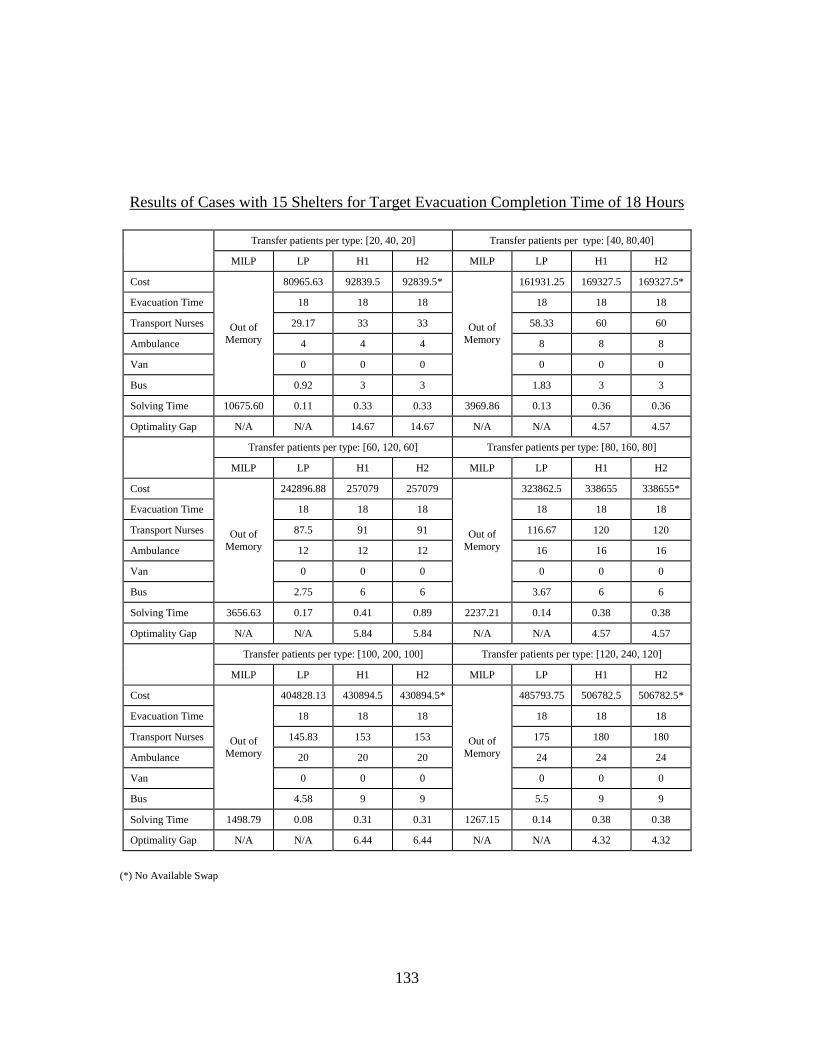
133

Results of Cases with 15 Shelters for Target Evacuation Completion Time of 18 Hours

Transfer patients per type: [20, 40, 20] Transfer patients per type: [40, 80,40]

MILP LP H1 H2 MILP LP H1 H2

Cost

Out of

Memory

80965.63 92839.5 92839.5*

Out of

Memory

161931.25 169327.5 169327.5*

Evacuation Time 18 18 18 18 18 18

Transport Nurses 29.17 33 33 58.33 60 60

Ambulance 4 4 4 8 8 8

Van 0 0 0 0 0 0

Bus 0.92 3 3 1.83 3 3

Solving Time 10675.60 0.11 0.33 0.33 3969.86 0.13 0.36 0.36

Optimality Gap N/A N/A 14.67 14.67 N/A N/A 4.57 4.57

Transfer patients per type: [60, 120, 60] Transfer patients per type: [80, 160, 80]

MILP LP H1 H2 MILP LP H1 H2

Cost

Out of

Memory

242896.88 257079 257079

Out of

Memory

323862.5 338655 338655*

Evacuation Time 18 18 18 18 18 18

Transport Nurses 87.5 91 91 116.67 120 120

Ambulance 12 12 12 16 16 16

Van 0 0 0 0 0 0

Bus 2.75 6 6 3.67 6 6

Solving Time 3656.63 0.17 0.41 0.89 2237.21 0.14 0.38 0.38

Optimality Gap N/A N/A 5.84 5.84 N/A N/A 4.57 4.57

Transfer patients per type: [100, 200, 100] Transfer patients per type: [120, 240, 120]

MILP LP H1 H2 MILP LP H1 H2

Cost

Out of

Memory

404828.13 430894.5 430894.5*

Out of

Memory

485793.75 506782.5 506782.5*

Evacuation Time 18 18 18 18 18 18

Transport Nurses 145.83 153 153 175 180 180

Ambulance 20 20 20 24 24 24

Van 0 0 0 0 0 0

Bus 4.58 9 9 5.5 9 9

Solving Time 1498.79 0.08 0.31 0.31 1267.15 0.14 0.38 0.38

Optimality Gap N/A N/A 6.44 6.44 N/A N/A 4.32 4.32

(*) No Available Swap

134

Transfer patients per type: [40, 20, 20] Transfer patients per type: [80, 40, 40]

MILP LP H1 H2 MILP LP H1 H2

Cost 133786.5 133178.13 145725 145725

Out of Memory

266356.25 276967.5 276967.5*

Evacuation Time 18 18 18 18 18 18 18

Transport Nurses 46 45.83 50 50 91.67 95 95

Ambulance 8 8 8 8 16 16 16

Van 0 0 0 0 0 0 0

Bus 1 0.58 2 2 1.17 3 3

Solving Time 9416.47 0.09 0.33 0.78 8231.39 0.09 0.33 0.33

Optimality Gap N/A N/A 9.42 9.42 N/A N/A 3.98 3.98

Transfer patients per type: [120, 60, 60] Transfer patients per type: [160, 80, 80]

MILP LP H1 H2 MILP LP H1 H2

Cost

Out of Memory

399534.38 417042 417042*

Out of Memory

532712.5 555316.5 555316.5

Evacuation Time 18 18 18 18 18 18

Transport Nurses 137.5 143 143 183.33 191 191

Ambulance 24 24 24 32 32 32

Van 0 0 0 0 0 0

Bus 1.75 4 4 2.33 5 5

Solving Time 5193.55 0.08 0.31 0.31 6163.45 0.14 0.38 1.39

Optimality Gap N/A N/A 4.38 4.38 N/A N/A 4.24 4.24

Transfer patients per type: [200, 100, 100] Transfer patients per type: [240, 120, 120]

MILP LP H1 H2 MILP LP H1 H2

Cost

Out of

Memory

665890.63 692847 692847

Out of

Memory

799068.75 829177.5 829177.5*

Evacuation Time 18 18 18 18 18 18

Transport Nurses 229.17 238 238 275 285 285

Ambulance 40 40 40 48 48 48

Van 0 0 0 0 0 0

Bus 2.92 6 6 3.5 7 7

Solving Time 4146.86 0.11 0.33 0.81 1751.36 0.17 0.42 0.42

Optimality Gap N/A N/A 4.05 4.05 N/A N/A 3.77 3.77

(*) No Available Swap

135

Transfer patients per type: [30, 30, 20] Transfer patients per type: [60, 60, 40]

MILP LP H1 H2 MILP LP H1 H2

Cost 108334.5 107071.88 115185 115185*

Out of Memory

214143.75 218287.5 218287.5*

Evacuation Time 18 18 18 18 18 18 18

Transport Nurses 38 37.5 40 40 75 75 75

Ambulance 6 6 6 6 12 12 12

Van 0 0 0 0 0 0 0

Bus 1 0.75 2 2 1.5 3 3

Solving Time 2978.28 0.08 0.30 0.30 15258.76 0.09 0.33 0.33

Optimality Gap N/A N/A 7.58 7.58 N/A N/A 1.94 1.94

Transfer patients per type: [90, 90, 60] Transfer patients per type: [120, 120, 80]

MILP LP H1 H2 MILP LP H1 H2

Cost

Out of Memory

321215.63 330510 330510* 428287.5 428287.5 433012.5 433012.5*

Evacuation Time 18 18 18 18 18 18 18

Transport Nurses 112.5 115 115 150 150 150 150

Ambulance 18 18 18 24 24 24 24

Van 0 0 0 0 0 0 0

Bus 2.25 4 4 3 3 5 5

Solving Time 6553.15 0.14 0.39 0.39 0.92 0.16 0.39 0.39

Optimality Gap N/A N/A 2.89 2.89 N/A N/A 1.10 1.10

Transfer patients per type: [150, 150, 100] Transfer patients per type: [180, 180, 120]

MILP LP H1 H2 MILP LP H1 H2

Cost

Out of

Memory

535359.38 547035 547035*

Out of

Memory

642431.25 648937.5 648937.5*

Evacuation Time 18 18 18 18 18 18

Transport Nurses 187.5 190 190 225 225 225

Ambulance 30 30 30 36 36 36

Van 0 0 0 0 0 0

Bus 3.75 6 6 4.5 7 7

Solving Time 5134.20 0.17 0.39 0.39 1964.94 0.11 0.34 0.34

Optimality Gap N/A N/A 2.18 2.18 N/A N/A 1.01 1.01

(*) No Available Swap

136

Results of Cases with 3 Shelters for the Target Evacuation Completion Time of 24 Hours

Transfer patients per type: [20, 40, 20] Transfer patients per type: [40, 80,40]

MILP LP H1 H2 MILP LP H1 H2

Cost

Out of Memory

82022.92 91908 91908

Out of Memory

164045.83 172284 170340

Evacuation Time 24 24 24 24 24 24

Transport Nurses 29.17 32 32 58.33 61 60

Ambulance 3.33 4 4 6.67 7 7

Van 0 0 0 0 0 0

Bus 0.76 2 2 1.53 2 2

Solving Time 2332.72 0.02 0.10 1.39 2695.16 0.02 0.08 2.27

Optimality Gap N/A N/A 12.05 12.05 N/A N/A 5.02 3.84

Transfer patients per type: [60, 120, 60] Transfer patients per type: [80, 160, 80]

MILP LP H1 H2 MILP LP H1 H2

Cost

Out of

Memory

246068.75 267480 264936

Out of

Memory

328091.67 342624 340080

Evacuation Time 24 24 24 23 23 23

Transport Nurses 87.5 95 94 116.67 121 120

Ambulance 10 10 10 13.33 14 14

Van 0 0 0 0 0 0

Bus 2.29 4 4 3.06 4 4

Solving Time 3507.57 0.02 0.09 3.43 1541.50 0.02 0.09 1.03

Optimality Gap N/A N/A 8.70 7.67 N/A N/A 4.43 3.65

Transfer patients per type: [100, 200, 100] Transfer patients per type: [120, 240, 120]

MILP LP H1 H2 MILP LP H1 H2

Cost

Out of

Memory

410114.58 430932 430932

Out of

Memory

492137.5 509514 509514

Evacuation Time 24 24 24 24 24 24

Transport Nurses 145.83 153 153 175 181 181

Ambulance 16.67 17 17 20 20 20

Van 0 0 0 0 0 0

Bus 3.82 6 6 4.58 7 7

Solving Time 1212 0.02 0.08 3.16 1346.50 0.02 0.08 0.23

Optimality Gap N/A N/A 5.08 5.08 N/A N/A 3.53 3.53

137

Transfer patients per type: [40, 20, 20] Transfer patients per type: [80, 40, 40]

MILP LP H1 H2 MILP LP H1 H2

Cost

Out of

Memory

135214.58 138774 138774

Out of

Memory

270429.17 273198 273198

Evacuation Time 24 24 24 24 24 24

Transport Nurses 45.83 46 46 91.67 92 92

Ambulance 6.67 7 7 13.33 14 14

Van 0 0 0 0 0 0

Bus 0.49 1 1 0.97 1 1

Solving Time 34892.16 0.02 0.09 1.33 2318.41 0.02 0.09 1.22

Optimality Gap N/A N/A 2.63 2.63 N/A N/A 1.02 1.02

Transfer patients per type: [120, 60, 60] Transfer patients per type: [160, 80, 80]

MILP LP H1 H2 MILP LP H1 H2

Cost

Out of

Memory

405643.75 423192 423192

Out of

Memory

540858.33 546546 546546

Evacuation Time 24 24 24 24 24 24

Transport Nurses 137.5 143 143 183.33 184 184

Ambulance 20 20 20 26.67 27 27

Van 0 0 0 0 0 0

Bus 1.46 4 4 1.94 3 3

Solving Time 3752.88 0.02 0.11 1.08 1723.57 0.02 0.09 1.67

Optimality Gap N/A N/A 4.33 4.33 N/A N/A 1.05 1.05

Transfer patients per type: [200, 100, 100] Transfer patients per type: [240, 120, 120]

MILP LP H1 H2 MILP LP H1 H2

Cost

Out of

Memory

676072.92 691890 689946

Out of

Memory

811287.5 820638 820638

Evacuation Time 24 24 24 24 24 24

Transport Nurses 229.17 235 234 275 277 277

Ambulance 33.33 34 34 40 40 40

Van 0 0 0 0 0 0

Bus 2.43 3 3 2.92 5 5

Solving Time 1800.43 0.02 0.09 1.91 1718.55 0.02 0.09 0.45

Optimality Gap N/A N/A 2.34 2.05 N/A N/A 1.15 1.15

138

Transfer patients per type: [30, 30, 20] Transfer patients per type: [60, 60, 40]

MILP LP H1 H2 MILP LP H1 H2

Cost 110022 108618.75 118998 118998 217850 217237.5 226332 226332*

Evacuation Time 24 24 24 24 24 24 24 24

Transport Nurses 38 37.5 42 42 75 75 78 78

Ambulance 5 5 5 5 10 10 10 10

Van 0 0 0 0 1 0 0 0

Bus 1 0.63 1 1 1 1.25 2 2

Solving Time 11.02 0.02 0.09 0.52 1585.43 0.02 0.08 0.08

Optimality Gap N/A N/A 9.56 9.56 N/A N/A 4.19 4.19

Transfer patients per type: [90, 90, 60] Transfer patients per type: [120, 120, 80]

MILP LP H1 H2 MILP LP H1 H2

Cost

Out of

Memory

325856.25 340242 338298 434850 434475 447576 447576*

Evacuation Time 24 24 24 24 24 24 24

Transport Nurses 112.5 118 117 150 150 154 154

Ambulance 15 15 15 20 20 20 20

Van 0 0 0 0 0 0 0

Bus 1.88 3 3 3 2.5 4 4

Solving Time 4357.14 0.02 0.09 0.88 60.64 0.02 0.08 0.08

Optimality Gap N/A N/A 4.42 3.82 N/A N/A 3.02 3.02

Transfer patients per type: [150, 150, 100] Transfer patients per type: [180, 180, 120]

MILP LP H1 H2 MILP LP H1 H2

Cost

Out of

Memory

543093.75 561648 558648

Out of

Memory

651712.5 661782 661782*

Evacuation Time 24 24 24 24 24 24

Transport Nurses 187.5 192 192 225 228 228

Ambulance 25 27 26 30 30 30

Van 0 0 0 0 0 0

Bus 3.13 4 4 3.75 5 5

Solving Time 2386.90 0.02 0.09 1.45 2655.85 0.02 0.09 0.09

Optimality Gap N/A N/A 3.42 2.86 N/A N/A 1.55 1.55

(*) No Available Swap

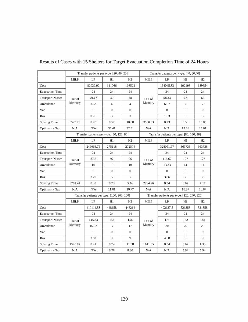
139

Results of Cases with 15 Shelters for Target Evacuation Completion Time of 24 Hours

Transfer patients per type: [20, 40, 20] Transfer patients per type: [40, 80,40]

MILP LP H1 H2 MILP LP H1 H2

Cost

Out of

Memory

82022.92 111066 108522

Out of

Memory

164045.83 192198 189654

Evacuation Time 24 24 24 24 24 24

Transport Nurses 29.17 39 38 58.33 67 66

Ambulance 3.33 4 4 6.67 7 7

Van 0 0 0 0 0 0

Bus 0.76 3 3 1.53 5 5

Solving Time 3523.75 0.20 0.52 10.80 3560.83 0.23 0.56 10.83

Optimality Gap N/A N/A 35.41 32.31 N/A N/A 17.16 15.61

Transfer patients per type: [60, 120, 60] Transfer patients per type: [80, 160, 80]

MILP LP H1 H2 MILP LP H1 H2

Cost

Out of

Memory

246068.75 275118 272574

Out of

Memory

328091.67 363738 363738

Evacuation Time 24 24 24 24 24 24

Transport Nurses 87.5 97 96 116.67 127 127

Ambulance 10 10 10 13.33 14 14

Van 0 0 0 0 0 0

Bus 2.29 5 5 3.06 7 7

Solving Time 3701.44 0.33 0.73 5.16 2234.26 0.34 0.67 7.17

Optimality Gap N/A N/A 11.81 10.77 N/A N/A 10.87 10.87

Transfer patients per type: [100, 200, 100] Transfer patients per type: [120, 240, 120]

MILP LP H1 H2 MILP LP H1 H2

Cost

Out of

Memory

410114.58 448158 446214

Out of

Memory

492137.5 521358 521358

Evacuation Time 24 24 24 24 24 24

Transport Nurses 145.83 157 156 175 182 182

Ambulance 16.67 17 17 20 20 20

Van 0 0 0 0 0 0

Bus 3.82 9 9 4.58 9 9

Solving Time 1545.87 0.41 0.74 11.58 1611.85 0.34 0.67 1.33

Optimality Gap N/A N/A 9.28 8.80 N/A N/A 5.94 5.94

140

Transfer patients per type: [40, 20, 20] Transfer patients per type: [80, 40, 40]

MILP LP H1 H2 MILP LP H1 H2

Cost

Out of

Memory

135214.58 163920 160626

Out of

Memory

270429.17 298200 295656

Evacuation Time 24 24 24 24 24 24

Transport Nurses 45.83 55 54 91.67 100 99

Ambulance 6.67 7 7 13.33 14 14

Van 0 0 0 0 0 0

Bus 0.49 4 3 0.97 4 4

Solving Time 2949.87 0.23 0.55 12.69 4010.68 0.17 0.49 5.18

Optimality Gap N/A N/A 21.23 18.79 N/A N/A 10.27 9.33

Transfer patients per type: [120, 60, 60] Transfer patients per type: [160, 80, 80]

MILP LP H1 H2 MILP LP H1 H2

Cost

Out of Memory

405643.75 445650 445650

Out of Memory

540858.33 585162 581868

Evacuation Time 24 24 24 24 24 24

Transport Nurses 137.5 150 150 183.33 198 197

Ambulance 20 20 20 26.67 27 27

Van 0 0 0 0 0 0

Bus 1.46 7 7 1.94 7 6

Solving Time 6979.16 0.30 0.61 6.70 5505.85 0.38 0.70 14.35

Optimality Gap N/A N/A 9.86 9.86 N/A N/A 8.19 7.58

Transfer patients per type: [200, 100, 100] Transfer patients per type: [240, 120, 120]

MILP LP H1 H2 MILP LP H1 H2

Cost

Out of Memory

676072.92 718098 718098

Out of Memory

811287.5 853266 853266

Evacuation Time 24 24 24 24 24 24

Transport Nurses 229.17 242 242 275 289 289

Ambulance 33.33 34 34 40 40 40

Van 0 0 0 0 0 0

Bus 2.43 7 7 2.92 7 7

Solving Time 2821.30 0.17 0.49 11.03 2328.39 0.33 0.64 1.97

Optimality Gap N/A N/A 6.22 6.22 N/A N/A 5.17 5.17

141

Transfer patients per type: [30, 30, 20] Transfer patients per type: [60, 60, 40]

MILP LP H1 H2 MILP LP H1 H2

Cost

Out of Memory

108618.75 125748 125748

Out of Memory

217237.5 232170 232170*

Evacuation Time 24 24 24 24 24 24

Transport Nurses 37.5 42 42 75 80 80

Ambulance 5 6 6 10 10 10

Van 0 0 0 0 0 0

Bus 0.63 2 2 1.3 3 3

Solving Time 29312.49 0.20 0.53 7.87 14309.96 0.20 0.52 0.52

Optimality Gap N/A N/A 15.77 15.77 N/A N/A 6.87 6.87

Transfer patients per type: [90, 90, 60] Transfer patients per type: [120, 120, 80]

MILP LP H1 H2 MILP LP H1 H2

Cost

Out of

Memory

325856.25 358212 354918

Out of

Memory

434475 441150 441150

Evacuation Time 24 24 24 24 24 24

Transport Nurses 112.5 123 122 150 150 150

Ambulance 15 15 15 20 20 20

Van 0 0 0 0 0 0

Bus 1.88 6 5 2.5 5 5

Solving Time 5970.91 0.38 0.69 5.82 9090.53 0.38 0.69 6.89

Optimality Gap N/A N/A 9.93 8.92 N/A N/A 1.54 1.54

Transfer patients per type: [150, 150, 100] Transfer patients per type: [180, 180, 120]

MILP LP H1 H2 MILP LP H1 H2

Cost

Out of Memory

543093.75 567786 567786

Out of Memory

651712.5 684396 684396

Evacuation Time 24 24 24 24 24 24

Transport Nurses 187.5 194 194 225 234 234

Ambulance 25 25 25 30 30 30

Van 0 0 0 0 0 0

Bus 3.13 7 7 3.75 10 10

Solving Time 5517.21 0.31 0.63 1.94 3654.33 0.36 0.67 2.68

Optimality Gap N/A N/A 4.55 4.55 N/A N/A 5.02 5.02

(*) No Available Swap

142

Results of Cases with 3 Shelters for the Target Evacuation Completion Time of 30 Hours

Transfer patients per type: [20, 40, 20] Transfer patients per type: [40, 80,40]

MILP LP H1 H2 MILP LP H1 H2

Cost

Out of Memory

79787.11 95137.5 95137.5

Out of Memory

159574.22 175185 175185

Evacuation Time 30 30 30 30 30 30

Transport Nurses 29.17 35 35 58.33 64 64

Ambulance 2.5 3 3 5 5 5

Van 0 0 0 0 0 0

Bus 0.57 1 1 1.15 2 2

Solving Time 1688.57 0.03 0.16 4.14 1811.71 0.06 0.17 1.38

Optimality Gap N/A N/A 19.24 19.24 N/A N/A 9.78 9.78

Transfer patients per type: [60, 120, 60] Transfer patients per type: [80, 160, 80]

MILP LP H1 H2 MILP LP H1 H2

Cost

Out of

Memory

239361.33 255382.5 255382.5

Out of

Memory

319148.44 335430 335430

Evacuation Time 30 30 30 30 30 30

Transport Nurses 87.5 93 93 116.67 122 122

Ambulance 7.5 8 8 10 10 10

Van 0 0 0 0 0 0

Bus 1.72 3 3 2.29 4 4

Solving Time 1077.67 0.03 0.13 3.11 2097.44 0.03 0.11 0.81

Optimality Gap N/A N/A 6.69 6.69 N/A N/A 5.10 5.10

Transfer patients per type: [100, 200, 100] Transfer patients per type: [120, 240, 120]

MILP LP H1 H2 MILP LP H1 H2

Cost

Out of Memory

398935.55 407820 407820

Out of Memory

478722.66 493537.5 491047.5

Evacuation Time 30 30 30 30 30 30

Transport Nurses 145.83 148 148 175 180 179

Ambulance 12.5 13 13 15 15 15

Van 0 0 0 0 0 0

Bus 2.86 4 4 3.44 5 5

Solving Time 1032.34 0.02 0.11 1.98 781.04 0.03 0.13 0.78

Optimality Gap N/A N/A 2.23 2.23 N/A N/A 3.09 2.57

143

Transfer patients per type: [40, 20, 20] Transfer patients per type: [80, 40, 40]

MILP LP H1 H2 MILP LP H1 H2

Cost 132427.5 131466.8 139207.5 139207.5 263917.5 262933.59 272677.5 272677.5

Evacuation Time 30 30 30 30 30 30 30 30

Transport Nurses 46 45.83 48 48 92 91.67 96 96

Ambulance 5 5 5 5 10 10 10 10

Van 0 0 0 0 0 0 0 0

Bus 1 0.36 1 1 1 0.73 1 1

Solving Time 9.14 0.02 0.09 1.06 17.62 0.03 0.13 0.73

Optimality Gap N/A N/A 5.89 5.89 N/A N/A 3.71 3.71

Transfer patients per type: [120, 60, 60] Transfer patients per type: [160, 80, 80]

MILP LP H1 H2 MILP LP H1 H2

Cost

Out of

Memory

394400.39 411885 409395

Out of

Memory

525867.19 535552.5 532125

Evacuation Time 30 30 30 30 30 30

Transport Nurses 137.5 144 143 183.33 186 185

Ambulance 15 15 15 20 20 20

Van 0 0 0 0 0 0

Bus 1.09 2 2 1.46 3 2

Solving Time 2207.97 0.03 0.11 1.39 1685.56 0.03 0.25 0.73

Optimality Gap N/A N/A 4.43 3.8 N/A N/A 1.84 1.19

Transfer patients per type: [200, 100, 100] Transfer patients per type: [240, 120, 120]

MILP LP H1 H2 MILP LP H1 H2

Cost

Out of

Memory

657333.98 672712.5 672712.5

Out of

Memory

788800.78 810720 808230

Evacuation Time 30 30 30 30 30 30

Transport Nurses 229.17 235 235 275 283 282

Ambulance 25 25 25 30 30 30

Van 0 0 0 0 0 0

Bus 1.82 3 3 2.19 4 4

Solving Time 1555.77 0.03 0.11 1.41 886.35 0.03 0.13 0.59

Optimality Gap N/A N/A 2.34 2.34 N/A N/A 2.78 2.46

144

Transfer patients per type: [30, 30, 20] Transfer patients per type: [60, 60, 40]

MILP LP H1 H2 MILP LP H1 H2

Cost

Out of Memory

105626.95 110557.5 110557.5

Out of Memory

211253.91 215377.5 215377.5

Evacuation Time 30 30 30 30 30 30

Transport Nurses 37.5 38 38 75 76 76

Ambulance 3.75 4 4 7.5 8 8

Van 0 0 0 0 0 0

Bus 0.47 1 1 0.94 1 1

Solving Time 1342.28 0.02 0.09 2.45 1113.88 0.02 0.11 2.58

Optimality Gap N/A N/A 4.67 4.67 N/A N/A 1.95 1.95

Transfer patients per type: [90, 90, 60] Transfer patients per type: [120, 120, 80]

MILP LP H1 H2 MILP LP H1 H2

Cost

Out of

Memory

316880.86 331252.5 331252.5 422625 422507.81 435412.5 435412.5

Evacuation Time 30 30 30 30 30 30 30

Transport Nurses 112.5 116 116 150 150 155 155

Ambulance 11.25 12 12 15 15 15 15

Van 0 0 0 0 0 0 0

Bus 1.41 3 3 2 1.88 3 3

Solving Time 906.07 0.03 0.13 2.97 0.25 0.03 0.13 0.73

Optimality Gap N/A N/A 4.54 4.54 N/A N/A 3.05 3.05

Transfer patients per type: [150, 150, 100] Transfer patients per type: [180, 180, 120]

MILP LP H1 H2 MILP LP H1 H2

Cost

Out of

Memory

528134.77 543480 543480

Out of

Memory

633761.72 649500 649500

Evacuation Time 30 30 30 30 30 30

Transport Nurses 187.5 192 192 225 230 230

Ambulance 18.75 19 19 22.5 23 23

Van 0 0 0 0 0 0

Bus 2.43 4 4 2.81 4 4

Solving Time 1124.39 0.03 0.11 2.27 931.98 0.02 0.11 1.20

Optimality Gap N/A N/A 2.91 2.91 N/A N/A 2.48 2.48

145

Results of Cases with 15 Shelters for Target Evacuation Completion Time of 30 Hours

Transfer patients per type: [20, 40, 20] Transfer patients per type: [40, 80,40]

MILP LP H1 H2 MILP LP H1 H2

Cost

Out of

Memory

79787.11 97875 97875

Out of

Memory

159574.22 183592.5 181102.5

Evacuation Time 30 30 30 30 30 30

Transport Nurses 29.17 35 35 58.33 67 66

Ambulance 2.5 3 3 5 5 5

Van 0 0 0 0 0 0

Bus 0.57 2 2 1.15 3 3

Solving Time 1975.41 0.59 1.00 10.20 1805.18 0.70 1.09 5.72

Optimality Gap N/A N/A 22.67 22.67 N/A N/A 15.05 13.49

Transfer patients per type: [60, 120, 60] Transfer patients per type: [80, 160, 80]

MILP LP H1 H2 MILP LP H1 H2

Cost

Out of Memory

239361.33 268927.5 266437.5

Out of Memory

319148.44 341857.5 339367.5

Evacuation Time 30 30 30 30 30 30

Transport Nurses 87.5 96 95 116.67 123 122

Ambulance 7.5 8 8 10 10 10

Van 0 0 0 0 0 0

Bus 1.72 5 5 2.29 5 5

Solving Time 1233.97 0.66 1.05 12.97 1227.23 0.69 1.09 5.11

Optimality Gap N/A N/A 12.35 11.31 N/A N/A 7.11 6.34

Transfer patients per type: [100, 200, 100] Transfer patients per type: [120, 240, 120]

MILP LP H1 H2 MILP LP H1 H2

Cost

Out of Memory

398935.55 434152.5 430725

Out of Memory

478722.66 515752.5 513262.5

Evacuation Time 30 30 30 30 30 30

Transport Nurses 145.83 156 155 175 186 185

Ambulance 12.5 13 13 15 15 15

Van 0 0 0 0 0 0

Bus 2.86 7 6 3.44 7 7

Solving Time 924.03 0.72 1.13 10.44 1009.58 0.75 1.42 4.33

Optimality Gap N/A N/A 8.83 7.97 N/A N/A 7.34 7.22

146

Transfer patients per type: [40, 20, 20] Transfer patients per type: [80, 40, 40]

MILP LP H1 H2 MILP LP H1 H2

Cost

Out of

Memory

131466.80 145125 142635

Out of

Memory

262933.59 287512.5 285022.5

Evacuation Time 30 30 30 30 30 30

Transport Nurses 45.83 50 49 91.67 100 99

Ambulance 5 5 5 10 10 10

Van 0 0 0 0 0 0

Bus 0.37 2 2 0.73 3 3

Solving Time 19273.91 0.58 1.19 6.33 4379.13 0.66 1.05 4.78

Optimality Gap N/A N/A 10.39 8.50 N/A N/A 9.35 8.4

Transfer patients per type: [120, 60, 60] Transfer patients per type: [160, 80, 80]

MILP LP H1 H2 MILP LP H1 H2

Cost

Out of

Memory

394400.39 423030 419602.5

Out of

Memory

525867.19 557347.5 554857.5

Evacuation Time 30 30 30 30 30 30

Transport Nurses 137.5 147 146 183.33 194 193

Ambulance 15 15 15 20 20 20

Van 0 0 0 0 0 0

Bus 1.09 4 3 1.46 5 5

Solving Time 1894.70 0.59 0.97 7.74 2803.00 0.34 0.77 2.52

Optimality Gap N/A N/A 7.26 6.39 N/A N/A 5.99 5.51

Transfer patients per type: [200, 100, 100] Transfer patients per type: [240, 120, 120]

MILP LP H1 H2 MILP LP H1 H2

Cost

Out of Memory

657333.98 690300 690300

Out of Memory

788800.78 820837.5 820837.5

Evacuation Time 30 30 30 30 30 30

Transport Nurses 229.17 240 240 275 285 285

Ambulance 25 25 25 30 30 30

Van 0 0 0 0 0 0

Bus 1.82 4 4 2.19 5 5

Solving Time 3586.39 0.86 1.25 6.86 1603.67 0.75 1.14 4.48

Optimality Gap N/A N/A 5.02 5.02 N/A N/A 4.06 4.06

147

Transfer patients per type: [30, 30, 20] Transfer patients per type: [60, 60, 40]

MILP LP H1 H2 MILP LP H1 H2

Cost

Out of

Memory

105626.95 117412.5 113985

Out of

Memory

211253.91 229950 226522.5

Evacuation Time 30 30 30 30 30 30

Transport Nurses 37.5 40 40 75 80 79

Ambulance 3.75 4 4 7.5 8 8

Van 0 0 0 0 0 0

Bus 0.47 3 2 0.94 4 3

Solving Time 2598.41 0.36 0.75 10.60 1536.33 0.75 1.14 10.61

Optimality Gap N/A N/A 11.16 7.91 N/A N/A 8.85 7.23

Transfer patients per type: [90, 90, 60] Transfer patients per type: [120, 120, 80]

MILP LP H1 H2 MILP LP H1 H2

Cost

Out of

Memory

316880.86 339922.5 339922.5 422625 422507.81 439950 439950

Evacuation Time 30 30 30 30 30 30 30

Transport Nurses 112.5 119 119 150 150 155 155

Ambulance 11.25 12 12 15 15 15 15

Van 0 0 0 0 0 0 0

Bus 1.41 3 3 2 1.88 4 4

Solving Time 1174.94 0.72 1.11 10.91 7.77 0.55 0.92 2.67

Optimality Gap N/A N/A 7.27 7.27 N/A N/A 4.13 4.13

Transfer patients per type: [150, 150, 100] Transfer patients per type: [180, 180, 120]

MILP LP H1 H2 MILP LP H1 H2

Cost

Out of Memory

528134.77 551797.5 551797.5

Out of Memory

633761.72 661492.5 659002.5

Evacuation Time 30 30 30 30 30 30

Transport Nurses 187.5 194 194 225 232 231

Ambulance 18.75 19 19 22.5 23 23

Van 0 0 0 0 0 0

Bus 2.34 5 5 2.81 7 7

Solving Time 1971.69 0.67 1.06 10.03 1285.99 0.72 1.11 6.66

Optimality Gap N/A N/A 4.48 4.48 N/A N/A 4.38 3.98

148

Results of Cases with 3 Shelters for the Target Evacuation Completion Time of 36 Hours

Transfer patients per type: [20, 40, 20] Transfer patients per type: [40, 80,40]

MILP LP H1 H2 MILP LP H1 H2

Cost

Out of

Memory

79922.92 88185 88185

Out of

Memory

159845.83 167670 167670

Evacuation Time 36 36 36 36 36 36

Transport Nurses 29.17 30 30 58.33 60 60

Ambulance 2.2 3 3 4.44 5 5

Van 0 0 0 0 0 0

Bus 0.51 1 1 1.02 2 2

Solving Time 3445.15 0.02 0.14 2.95 2754.88 0.03 0.13 3.97

Optimality Gap N/A N/A 10.34 10.34 N/A N/A 4.89 4.89

Transfer patients per type: [60, 120, 60] Transfer patients per type: [80, 160, 80]

MILP LP H1 H2 MILP LP H1 H2

Cost

Out of

Memory

239768.75 263187 261315

Out of

Memory

319691.67 342075 339603

Evacuation Time 36 36 36 36 36 36

Transport Nurses 87.5 96 95 116.67 125 124

Ambulance 6.67 7 7 8.89 9 9

Van 0 0 0 0 0 0

Bus 1.53 3 3 2.04 3 3

Solving Time 2151.61 0.03 0.13 5.27 6283.53 0.03 0.13 3.97

Optimality Gap N/A N/A 9.77 8.99 N/A N/A 7.00 6.23

Transfer patients per type: [100, 200, 100] Transfer patients per type: [120, 240, 120]

MILP LP H1 H2 MILP LP H1 H2

Cost

Out of

Memory

399614.58 420444 418572

Out of

Memory

479537.5 497460 497460

Evacuation Time 36 36 36 36 36 36

Transport Nurses 145.83 152 151 175 180 180

Ambulance 11.11 12 12 13.33 14 14

Van 0 0 0 0 0 0

Bus 2.55 4 4 3.06 4 4

Solving Time 1640.78 0.03 0.13 4.33 1507.65 0.03 0.14 1.69

Optimality Gap N/A N/A 5.21 4.74 N/A N/A 3.74 3.74

149

Transfer patients per type: [40, 20, 20] Transfer patients per type: [80, 40, 40]

MILP LP H1 H2 MILP LP H1 H2

Cost

Out of Memory

131914.58 144753 144753 265449 263829.17 278481 278481

Evacuation Time 36 36 36 36 36 36 36

Transport Nurses 45.83 49 49 92 91.67 98 98

Ambulance 4.44 5 5 9 8.89 9 9

Van 0 0 0 0 0 0 0

Bus 0.32 1 1 1 0.65 1 1

Solving Time 2991.50 0.02 0.13 3.69 297.01 0.02 0.13 2.52

Optimality Gap N/A N/A 9.73 9.73 N/A N/A 5.55 5.55

Transfer patients per type: [120, 60, 60] Transfer patients per type: [160, 80, 80]

MILP LP H1 H2 MILP LP H1 H2

Cost

Out of

Memory

395743.75 419415 416943

Out of

Memory

527658.33 560415 558543

Evacuation Time 36 36 36 36 36 36

Transport Nurses 137.5 145 144 183.33 195 194

Ambulance 13.33 14 14 17.78 18 18

Van 0 0 0 0 0 0

Bus 0.97 3 3 1.30 3 3

Solving Time 1895.49 0.03 0.13 4.92 2327.17 0.03 0.13 4.75

Optimality Gap N/A N/A 5.98 5.36 N/A N/A 6.21 5.85

Transfer patients per type: [200, 100, 100] Transfer patients per type: [240, 120, 120]

MILP LP H1 H2 MILP LP H1 H2

Cost

Out of

Memory

659572.92 685539 685539

Out of

Memory

791487.5 823464 821592

Evacuation Time 36 36 36 36 36 36

Transport Nurses 229.17 237 237 275 287 286

Ambulance 22.22 23 23 26.67 27 27

Van 0 0 0 0 0 0

Bus 1.62 3 3 1.94 4 4

Solving Time 2114.81 0.02 0.13 4.24 1649.74 0.02 0.13 3.31

Optimality Gap N/A N/A 3.94 3.94 N/A N/A 4.04 3.80

150

Transfer patients per type: [30, 30, 20] Transfer patients per type: [60, 60, 40]

MILP LP H1 H2 MILP LP H1 H2

Cost

Out of Memory

105918.75 115533 115533

Out of Memory

211837.5 220041 220041

Evacuation Time 36 36 36 36 36 36

Transport Nurses 37.5 39 39 75 78 78

Ambulance 3.33 4 4 6.67 7 7

Van 0 0 0 0 0 0

Bus 0.42 1 1 0.83 1 1

Solving Time 2928.89 0.02 0.12 2.53 3507.79 0.02 0.13 2.66

Optimality Gap N/A N/A 9.08 9.08 N/A N/A 3.87 3.87

Transfer patients per type: [90, 90, 60] Transfer patients per type: [120, 120, 80]

MILP LP H1 H2 MILP LP H1 H2

Cost

Out of

Memory

317756.25 331074 331074*

Out of

Memory

423675 444207 444207

Evacuation Time 36 36 36 36 36 36

Transport Nurses 112.5 117 117 150 156 156

Ambulance 10 10 10 13.33 14 14

Van 0 0 0 0 0 0

Bus 1.25 2 2 1.67 3 3

Solving Time 5897.57 0.02 0.14 0.14 1865.43 0.03 0.13 1.86

Optimality Gap N/A N/A 4.19 4.19 N/A N/A 4.85 4.85

Transfer patients per type: [150, 150, 100] Transfer patients per type: [180, 180, 120]

MILP LP H1 H2 MILP LP H1 H2

Cost

Out of

Memory

529593.75 552840 552840

Out of

Memory

635512.5 638775 638775*

Evacuation Time 36 36 36 36 36 36

Transport Nurses 187.5 195 195 225 225 225

Ambulance 16.67 17 17 20 20 20

Van 0 0 0 0 0 0

Bus 2.08 4 4 2.5 3 3

Solving Time 3393.29 0.03 0.12 2.42 1852.52 0.03 0.14 0.14

Optimality Gap N/A N/A 4.39 4.39 N/A N/A 0.51 0.51

(*) No Available Swap

151

Results of Cases with 15 shelters for Target Evacuation Completion Time of 36 Hours

Transfer patients per type: [20, 40, 20] Transfer patients per type: [40, 80,40]

MILP LP H1 H2 MILP LP H1 H2

Cost

Out of

Memory

79922.92 94254 92382

Out of

Memory

159845.83 175539 175539

Evacuation Time 36 36 36 36 36 36

Transport Nurses 29.17 32 31 58.33 62 62

Ambulance 2.22 3 3 4.44 5 5

Van 0 0 0 0 0 0

Bus 0.51 2 2 1.02 3 3

Solving Time 2609.98 0.97 1.42 18.64 2534.15 0.84 1.31 25.47

Optimality Gap N/A N/A 17.93 15.59 N/A N/A 9.82 9.82

Transfer patients per type: [60, 120, 60] Transfer patients per type: [80, 160, 80]

MILP LP H1 H2 MILP LP H1 H2

Cost

Out of

Memory

239768.75 279525 277653

Out of

Memory

319691.67 358266 358266

Evacuation Time 36 36 36 36 36 36

Transport Nurses 87.5 100 99 116.67 128 128

Ambulance 6.67 7 7 8.88 9 9

Van 0 0 0 0 0 0

Bus 1.53 5 5 2.04 6 6

Solving Time 3338.49 1.05 1.50 31.57 5422.72 1.02 1.47 28.88

Optimality Gap N/A N/A 16.58 15.80 N/A N/A 12.07 12.07

Transfer patients per type: [100, 200, 100] Transfer patients per type: [120, 240, 120]

MILP LP H1 H2 MILP LP H1 H2

Cost

Out of Memory

399614.58 447123 447123

Out of Memory

479537.5 515070 515070

Evacuation Time 36 36 36 36 36 36

Transport Nurses 145.83 159 159 175 185 185

Ambulance 11.11 12 12 13.33 14 14

Van 0 0 0 0 0 0

Bus 2.55 7 7 3.06 6 6

Solving Time 2128.13 1.13 1.58 22.46 2747.48 1.13 1.58 14.71

Optimality Gap N/A N/A 11.89 11.89 N/A N/A 7.41 7.41

152

Transfer patients per type: [40, 20, 20] Transfer patients per type: [80, 40, 40]

MILP LP H1 H2 MILP LP H1 H2

Cost

Out of

Memory

131914.58 150822 150822

Out of

Memory

263829.17 287403 283806

Evacuation Time 36 36 36 36 36 36

Transport Nurses 45.83 51 51 91.67 99 98

Ambulance 4.44 5 5 8.89 9 9

Van 0 0 0 0 0 0

Bus 0.32 2 2 0.65 3 2

Solving Time 5308.81 0.75 1.22 22.27 59125.98 1.02 1.47 16.58

Optimality Gap N/A N/A 14.33 14.33 N/A N/A 8.94 7.57

Transfer patients per type: [120, 60, 60] Transfer patients per type: [160, 80, 80]

MILP LP H1 H2 MILP LP H1 H2

Cost

Out of

Memory

395743.75 423468 419871

Out of

Memory

527658.33 569556 567084

Evacuation Time 36 36 36 36 36 36

Transport Nurses 137.5 144 143 183.33 198 197

Ambulance 13.33 14 14 17.78 18 18

Van 0 0 0 0 0 0

Bus 0.97 4 3 1.30 4 4

Solving Time 3012.85 0.95 1.41 29.57 3110.46 0.88 1.33 34.93

Optimality Gap N/A N/A 7.01 6.10 N/A N/A 7.94 7.47

Transfer patients per type: [200, 100, 100] Transfer patients per type: [240, 120, 120]

MILP LP H1 H2 MILP LP H1 H2

Cost

Out of

Memory

659572.92 716487 712890

Out of

Memory

791487.5 839130 839130

Evacuation Time 36 36 36 36 36 36

Transport Nurses 229.17 246 245 275 290 290

Ambulance 22.22 23 23 26.67 27 27

Van 0 0 0 0 0 0

Bus 1.62 7 6 1.94 6 6

Solving Time 3517.06 0.55 1.00 21.36 2989.85 0.75 1.20 9.00

Optimality Gap N/A N/A 8.63 8.08 N/A N/A 6.02 6.02

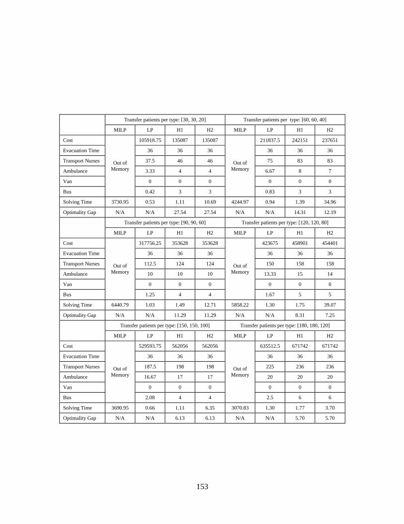
153

Transfer patients per type: [30, 30, 20] Transfer patients per type: [60, 60, 40]

MILP LP H1 H2 MILP LP H1 H2

Cost

Out of

Memory

105918.75 135087 135087

Out of

Memory

211837.5 242151 237651

Evacuation Time 36 36 36 36 36 36

Transport Nurses 37.5 46 46 75 83 83

Ambulance 3.33 4 4 6.67 8 7

Van 0 0 0 0 0 0

Bus 0.42 3 3 0.83 3 3

Solving Time 3730.95 0.53 1.11 10.69 4244.97 0.94 1.39 34.96

Optimality Gap N/A N/A 27.54 27.54 N/A N/A 14.31 12.19

Transfer patients per type: [90, 90, 60] Transfer patients per type: [120, 120, 80]

MILP LP H1 H2 MILP LP H1 H2

Cost

Out of

Memory

317756.25 353628 353628

Out of

Memory

423675 458901 454401

Evacuation Time 36 36 36 36 36 36

Transport Nurses 112.5 124 124 150 158 158

Ambulance 10 10 10 13.33 15 14

Van 0 0 0 0 0 0

Bus 1.25 4 4 1.67 5 5

Solving Time 6440.79 1.03 1.49 12.71 5858.22 1.30 1.75 39.07

Optimality Gap N/A N/A 11.29 11.29 N/A N/A 8.31 7.25

Transfer patients per type: [150, 150, 100] Transfer patients per type: [180, 180, 120]

MILP LP H1 H2 MILP LP H1 H2

Cost

Out of

Memory

529593.75 562056 562056

Out of

Memory

635512.5 671742 671742

Evacuation Time 36 36 36 36 36 36

Transport Nurses 187.5 198 198 225 236 236

Ambulance 16.67 17 17 20 20 20

Van 0 0 0 0 0 0

Bus 2.08 4 4 2.5 6 6

Solving Time 3690.95 0.66 1.11 6.35 3070.83 1.30 1.77 3.70

Optimality Gap N/A N/A 6.13 6.13 N/A N/A 5.70 5.70

154

Results of Cases with 3 Shelters for the Target Evacuation Completion Time of 42 Hours

Transfer patients per type: [20, 40, 20] Transfer patients per type: [40, 80,40]

MILP LP H1 H2 MILP LP H1 H2

Cost

Out of

Memory

79442.33 88444.5 88444.5

Out of

Memory

158884.66 168976.5 168976.5

Evacuation Time 42 42 42 42 42 42

Transport Nurses 29.17 31 31 58.33 62 62

Ambulance 1.82 2 2 3.64 4 4

Van 0 0 0 0 0 0

Bus 0.42 1 1 0.83 1 1

Solving Time 1363.07 0.05 0.20 3.16 1173.49 0.05 0.16 4.52

Optimality Gap N/A N/A 11.33 11.33 N/A N/A 6.35 6.35

Transfer patients per type: [60, 120, 60] Transfer patients per type: [80, 160, 80]

MILP LP H1 H2 MILP LP H1 H2

Cost

Out of

Memory

238326.99 257421 257421

Out of

Memory

317769.32 337953 337953

Evacuation Time 42 42 42 42 42 42

Transport Nurses 87.5 93 93 116.67 124 124

Ambulance 5.45 6 6 7.27 8 8

Van 0 0 0 0 0 0

Bus 1.25 2 2 1.67 2 2

Solving Time 964.88 0.03 0.14 4.42 825 0.06 0.17 5.11

Optimality Gap N/A N/A 8.01 8.01 N/A N/A 6.35 6.35

Transfer patients per type: [100, 200, 100] Transfer patients per type: [120, 240, 120]

MILP LP H1 H2 MILP LP H1 H2

Cost

Out of Memory

397211.65 426397.5 426397.5

Out of Memory

476653.98 484831.5 484831.5

Evacuation Time 42 42 42 42 42 42

Transport Nurses 145.83 155 155 175 177 177

Ambulance 9.09 10 10 10.91 11 11

Van 0 0 0 0 0 0

Bus 2.08 3 3 2.5 3 3

Solving Time 755.73 0.05 0.16 2.86 860.66 0.09 0.22 2.31

Optimality Gap N/A N/A 7.35 7.35 N/A N/A 1.72 1.72

155

Transfer patients per type: [40, 20, 20] Transfer patients per type: [80, 40, 40]

MILP LP H1 H2 MILP LP H1 H2

Cost

Out of

Memory

130988.92 148384.5 148384.5

Out of

Memory

261977.84 275752.5 275752.5

Evacuation Time 42 42 42 42 42 42

Transport Nurses 45.83 51 51 91.67 95 95

Ambulance 3.64 4 4 7.27 8 8

Van 0 0 0 0 0 0

Bus 0.27 1 1 0.53 1 1

Solving Time 1478.25 0.03 0.16 6.22 1065.60 0.05 0.16 6.11

Optimality Gap N/A N/A 13.28 13.28 N/A N/A 5.26 5.26

Transfer patients per type: [120, 60, 60] Transfer patients per type: [160, 80, 80]

MILP LP H1 H2 MILP LP H1 H2

Cost

Out of Memory

392966.76 407271 405399

Out of Memory

523955.68 549399 546927

Evacuation Time 42 42 42 42 42 42

Transport Nurses 137.5 143 142 183.33 192 191

Ambulance 10.91 11 11 14.55 15 15

Van 0 0 0 0 0 0

Bus 0.80 2 2 1.06 2 2

Solving Time 15043.49 0.05 0.17 5.70 1268.01 0.05 0.17 7.28

Optimality Gap N/A N/A 3.64 3.16 N/A N/A 4.86 4.38

Transfer patients per type: [200, 100, 100] Transfer patients per type: [240, 120, 120]

MILP LP H1 H2 MILP LP H1 H2

Cost

Out of

Memory

654944.6 675535.5 675535.5

Out of

Memory

785933.52 813870 810085.5

Evacuation Time 42 42 42 42 42 42

Transport Nurses 229.17 234 234 275 285 284

Ambulance 18.18 19 19 21.82 22 22

Van 0 0 0 0 0 0

Bus 1.33 3 3 1.59 4 3

Solving Time 1160.47 0.05 0.16 5.33 1098.88 0.06 0.17 3.50

Optimality Gap N/A N/A 3.14 3.14 N/A N/A 3.55 3.07

156

Transfer patients per type: [30, 30, 20] Transfer patients per type: [60, 60, 40]

MILP LP H1 H2 MILP LP H1 H2

Cost

Out of

Memory

105215.63 118414.5 118414.5

Out of

Memory

210431.25 228916.5 228916.5

Evacuation Time 42 42 42 42 42 42

Transport Nurses 37.5 41 41 75 82 82

Ambulance 2.73 3 3 5.45 6 6

Van 0 0 0 0 0 0

Bus 0.34 1 1 0.68 1 1

Solving Time 1747.37 0.03 0.19 5.16 962.87 0.03 0.14 6.64

Optimality Gap N/A N/A 12.54 12.54 N/A N/A 8.78 8.78

Transfer patients per type: [90, 90, 60] Transfer patients per type: [120, 120, 80]

MILP LP H1 H2 MILP LP H1 H2

Cost

Out of Memory

315646.88 330027 327555

Out of Memory

420862.5 435775.5 435775.5

Evacuation Time 42 42 42 42 42 42

Transport Nurses 112.5 116 115 150 154 154

Ambulance 8.18 9 9 10.91 11 11

Van 0 0 0 0 0 0

Bus 1.02 2 2 1.36 3 3

Solving Time 856.27 0.03 0.16 5.78 12044.97 0.05 0.17 6.20

Optimality Gap N/A N/A 4.56 3.77 N/A N/A 3.54 3.54

Transfer patients per type: [150, 150, 100] Transfer patients per type: [180, 180, 120]

MILP LP H1 H2 MILP LP H1 H2

Cost

Out of Memory

526078.13 546877.5 546877.5

Out of Memory

631293.75 655963.5 653491.5

Evacuation Time 42 42 42 42 42 42

Transport Nurses 187.5 195 195 225 233 232

Ambulance 13.64 14 14 16.36 17 17

Van 0 0 0 0 0 0

Bus 1.71 3 3 2.05 3 3

Solving Time 1228.64 0.05 0.17 7.06 1060.85 0.05 0.16 3.92

Optimality Gap N/A N/A 3.95 3.95 N/A N/A 3.91 3.52

157

Results of Cases with 15 Shelters for Target Evacuation Completion Time of 42 Hours

Transfer patients per type: [20, 40, 20] Transfer patients per type: [40, 80,40]

MILP LP H1 H2 MILP LP H1 H2

Cost

Out of

Memory

79442.33 97173 97173

Out of

Memory

158884.66 178833 178833

Evacuation Time 42 42 42 42 42 42

Transport Nurses 29.17 34 34 58.33 64 64

Ambulance 1.82 2 2 3.64 4 4

Van 0 0 0 0 0 0

Bus 0.42 2 2 0.83 2 2

Solving Time 3478.16 0.64 1.17 14.14 1698.28 0.61 1.14 21.03

Optimality Gap N/A N/A 22.32 22.32 N/A N/A 12.56 12.56

Transfer patients per type: [60, 120, 60] Transfer patients per type: [80, 160, 80]

MILP LP H1 H2 MILP LP H1 H2

Cost

Out of

Memory

238326.99 271693.5 271693.5

Out of

Memory

317769.32 346578 346578

Evacuation Time 42 42 42 42 42 42

Transport Nurses 87.5 98 98 116.67 124 124

Ambulance 5.45 6 6 7.27 8 8

Van 0 0 0 0 0 0

Bus 1.25 3 3 1.67 4 4

Solving Time 1740.75 0.56 1.09 15.27 1334.65 0.64 1.17 21.94

Optimality Gap N/A N/A 14.00 14.00 N/A N/A 9.07 9.07

Transfer patients per type: [100, 200, 100] Transfer patients per type: [120, 240, 120]

MILP LP H1 H2 MILP LP H1 H2

Cost

Out of Memory

397211.65 433894.5 433894.5

Out of Memory

476653.98 517089 517089

Evacuation Time 42 42 42 42 42 42

Transport Nurses 145.83 156 156 175 187 187

Ambulance 9.09 10 10 10.91 11 11

Van 0 0 0 0 0 0

Bus 2.08 5 5 2.5 6 6

Solving Time 1079.27 0.63 1.17 22.02 1437.63 0.64 1.17 8.81

Optimality Gap N/A N/A 9.24 9.24 N/A N/A 8.48 8.48

158

Transfer patients per type: [40, 20, 20] Transfer patients per type: [80, 40, 40]

MILP LP H1 H2 MILP LP H1 H2

Cost

Out of Memory

130988.92 157113 154641

Out of Memory

261977.84 285121.5 284521.5

Evacuation Time 42 42 42 42 42 42

Transport Nurses 45.83 54 53 91.67 97 97

Ambulance 3.64 4 4 7.27 8 8

Van 0 0 0 0 0 0

Bus 0.27 2 2 0.53 3 3

Solving Time 2083.64 0.49 1.03 26.77 1837.65 0.44 1.09 27.05

Optimality Gap N/A N/A 19.94 18.06 N/A N/A 8.83 8.61

Transfer patients per type: [120, 60, 60] Transfer patients per type: [160, 80, 80]

MILP LP H1 H2 MILP LP H1 H2

Cost

Out of

Memory

392966.76 425815.5 423343.5

Out of

Memory

523955.68 562999.5 560527.5

Evacuation Time 42 42 42 42 42 42

Transport Nurses 137.5 149 148 183.33 196 195

Ambulance 10.91 11 11 14.55 15 15

Van 0 0 0 0 0 0

Bus 0.80 3 3 1.06 3 3

Solving Time 3358.76 0.47 1.03 24.80 1988.30 0.36 0.89 29.39

Optimality Gap N/A N/A 8.36 7.73 N/A N/A 7.45 6.98

Transfer patients per type: [200, 100, 100] Transfer patients per type: [240, 120, 120]

MILP LP H1 H2 MILP LP H1 H2

Cost

Out of

Memory

654944.60 697224 694752

Out of

Memory

785933.52 832302 829830

Evacuation Time 42 42 42 42 42 42

Transport Nurses 229.17 242 241 275 291 290

Ambulance 18.18 19 19 21.82 22 22

Van 0 0 0 0 0 0

Bus 1.33 4 4 1.59 4 4

Solving Time 2426.15 0.39 1.09 26.51 1691.84 0.38 0.91 13.17

Optimality Gap N/A N/A 6.46 6.08 N/A N/A 5.90 5.59

159

Transfer patients per type: [30, 30, 20] Transfer patients per type: [60, 60, 40]

MILP LP H1 H2 MILP LP H1 H2

Cost

Out of Memory

105215.63 127143 127143

Out of Memory

210431.25 239373 236901

Evacuation Time 42 42 42 42 42 42

Transport Nurses 37.5 44 44 75 84 83

Ambulance 2.73 3 3 5.45 6 6

Van 0 0 0 0 0 0

Bus 0.34 2 2 0.68 2 2

Solving Time 2560.22 0.64 1.17 24.52 2698.96 0.42 0.95 27.10

Optimality Gap N/A N/A 20.84 20.84 N/A N/A 13.75 12.58

Transfer patients per type: [90, 90, 60] Transfer patients per type: [120, 120, 80]

MILP LP H1 H2 MILP LP H1 H2

Cost

Out of Memory

315646.88 341755.5 339283.5

Out of Memory

420862.5 446263.5 446263.5

Evacuation Time 42 42 42 42 42 42

Transport Nurses 112.5 119 118 150 158 158

Ambulance 8.18 9 9 10.91 11 11

Van 0 0 0 0 0 0

Bus 1.02 3 3 1.36 3 3

Solving Time 1390.37 0.45 1.16 27.70 8854.60 0.52 1.05 24.08

Optimality Gap N/A N/A 8.27 7.49 N/A N/A 6.04 6.04

Transfer patients per type: [150, 150, 100] Transfer patients per type: [180, 180, 120]

MILP LP H1 H2 MILP LP H1 H2

Cost

Out of Memory

526078.13 554190 554190

Out of Memory

631293.75 667732.5 665260.5

Evacuation Time 42 42 42 42 42 42

Transport Nurses 187.5 195 195 225 235 234

Ambulance 13.64 14 14 16.36 17 17

Van 0 0 0 0 0 0

Bus 1.71 4 4 2.05 5 5

Solving Time 2190.06 0.47 1.00 21.53 2164.82 0.58 1.14 13.41

Optimality Gap N/A N/A 5.34 5.34 N/A N/A 5.77 5.38

160

Appendix 2

Optimization Result Tables for Cases with Fixed Costs

Case 1 - Transfer patients per type: [40, 80, 40] & Bed/facility: [40, 80, 40] & 3 Shelters

Target Evacuation Time

≤ 12 ≤ 18 ≤ 24

LP H2 LP H2 LP H2

Cost 188458.33 195600 171541.67 175500 167312.5 173700

Evacuation Time 12 12 18 18 24 24

Transport Nurses 58.33 60 58.33 60 58.33 60

Ambulance 13.33 14 8 8 6.67 7

Van 0 0 0 0 0 0

Bus 3.06 4 1.33 2 1.53 2

Solving Time 0.01 0.27 0.02 0.17 0.02 2.05

Optimality Gap N/A 3.79 N/A 2.31 N/A 3.82

Target Evacuation Time

≤ 30 ≤ 36 ≤ 42

LP H2 LP H2 LP H2

Cost 162026.04 178100 160263.89 167100 157700.76 167350

Evacuation Time 30 30 36 36 42 42

Transport Nurses 58.33 64 58.33 60 58.33 62

Ambulance 5 5 4.44 5 3.64 4

Van 0 0 0 0 0 0

Bus 1.15 2 1.02 2 0.83 1

Solving Time 0.02 1.19 0.03 4.31 0.03 4.28

Optimality Gap N/A 9.92 N/A 4.27 N/A 6.12

161

Case 2 - Transfer patients per type: [160, 80, 80] & Bed/facility: [80, 40, 40] & 3 Shelters

Target Evacuation Time

≤ 12 ≤ 18 ≤ 24

LP H2 LP H2 LP H2

Cost 632583.33 642750 567416.67 576600 551125 555650

Evacuation Time 12 12 18 18 24 24

Transport Nurses 183.33 186 183.33 186 183.33 184

Ambulance 53.33 54 32 32 26.67 27

Van 0 0 0 0 0 0

Bus 3.89 5 2.33 4 1.94 3

Solving Time 0.01 0.34 0.02 1.22 0.03 1.22

Optimality Gap N/A 1.61 N/A 1.62 N/A 0.82

Target Evacuation Time

≤ 30 ≤ 36 ≤ 42

LP H2 LP H2 LP H2

Cost 530760.42 537100 523972.22 555250 514098.48 536500

Evacuation Time 30 30 36 36 42 42

Transport Nurses 183.33 185 183.33 194 183.33 191

Ambulance 20 20 17.78 18 14.55 15

Van 0 0 0 0 0 0

Bus 1.46 3 1.30 3 1.06 2

Solving Time 0.02 0.58 0.03 5.33 0.03 7.63

Optimality Gap N/A 1.19 N/A 5.97 N/A 4.36

162

Case 3 - Transfer patients per type: [20, 40, 20] & Bed/facility: [8, 16, 8] & 15 Shelters

Target Evacuation Time

≤ 12 ≤ 18 ≤ 24

LP H2 LP H2 LP H2

Cost 94229.17 108000 85770.83 92300 83656.25 110650

Evacuation Time 12 12 18 18 24 24

Transport Nurses 29.17 33 29.17 31 29.17 38

Ambulance 6.67 7 4 4 3.33 4

Van 0 0 0 0 0 0

Bus 1.53 4 0.92 2 0.76 3

Solving Time 0.05 0.98 0.11 0.34 0.22 10.3

Optimality Gap N/A 14.61 N/A 7.61 N/A 32.27

Target Evacuation Time

≤ 30 ≤ 36 ≤ 42

LP H2 LP H2 LP H2

Cost 81013.02 99100 80131.94 88500 78850.38 95900

Evacuation Time 30 30 36 36 42 42

Transport Nurses 29.17 35 29.17 30 29.17 34

Ambulance 2.5 3 2.22 3 1.82 2

Van 0 0 0 0 0 0

Bus 0.57 2 0.51 2 0.42 2

Solving Time 0.56 9.3 0.75 15.04 0.61 13.76

Optimality Gap N/A 22.33 N/A 10.44 N/A 21.62

163

Case 4 - Transfer patients per type: [40, 20, 20] & Bed/facility: [16, 8, 8] & 15 Shelters

Target Evacuation Time

≤ 12 ≤ 18 ≤ 24

LP H2 LP H2 LP H2

Cost 158145.83 165850 141854.17 154900 137781.25 163650

Evacuation Time 12 12 18 18 24 24

Transport Nurses 45.83 47 45.83 50 45.83 54

Ambulance 13.33 14 8 8 6.67 7

Van 0 0 0 0 0 0

Bus 0.97 3 0.58 2 0.49 3

Solving Time 0.05 1.13 0.09 1 0.25 11.73

Optimality Gap N/A 4.87 N/A 9.2 N/A 18.78

Target Evacuation Time

≤ 30 ≤ 36 ≤ 42

LP H2 LP H2 LP H2

Cost 132690.1 143900 130993.05 149100 128524.62 153900

Evacuation Time 30 30 36 36 42 42

Transport Nurses 45.83 49 45.83 51 45.83 54

Ambulance 5 5 4.44 5 3.64 4

Van 0 0 0 0 0 0

Bus 0.37 2 0.32 2 0.27 2

Solving Time 0.58 5.7 0.75 22.02 0.45 29.82

Optimality Gap N/A 8.45 N/A 13.82 N/A 19.74

164

Appendix 3

Optimization Result Tables for Weighted Time Objective

Result Tables for Percentage Level of 2

Bed/facility= [40, 80, 40]

Transfer patients per type

[20,40,20] [40,80,40] [60,120,60] [80,160,80] [100,200,100] [120,240,120]

Cost

Infeasible Case

167196 250722 334598 418124

Out of Memory

Evacuation Time 22 22 22 22

Weighted Time 9044 6674 9840 10784

Transport Nurses 59 88 117 146

Ambulance 7 10 14 17

Van 0 0 1 1

Bus 2 7 7 12

Solving Time 0.30 19.67 1.44 3.86 3.11 13576.74

Bed/facility= [80, 40, 40]

Transfer patients per type

[40,20,20] [80,40,40] [120,60,60] [160,80,80] [200,100,100] [240,120,120]

Cost 137724 275448 413172 551646 689370

Out of

Memory

Evacuation Time 22 22 22 22 22

Weighted Time 3484 6968 10452 13768 17252

Transport Nurses 46 92 138 184 230

Ambulance 7 14 21 28 35

Van 0 0 0 0 0

Bus 2 4 6 9 11

Solving Time 1.47 1.98 2.09 1.52 1.24 3931.93

Bed/facility= [60, 60, 40]

Transfer patients per type

[30,30,20] [60,60,40] [90,90,60] [120,120,80] [150,150,100] [180,180,120]

Cost 110772 221400 332172 443100 553872 664450

Evacuation Time 22 22 22 22 22 22

Weighted Time 3024 5628 8652 10910 13934 16444

Transport Nurses 38 75 113 150 188 225

Ambulance 5 10 15 21 26 32

Van 0 1 1 0 0 2

Bus 2 6 8 10 12 11

Solving Time 0.16 1.63 1.64 0.53 1.66 12.81

165

Bed/facility= [8, 16, 8]

Transfer patients per type

[20,40,20] [40,80,40] [60,120,60] [80,160,80] [100,200,100] [120,240,120]

Cost

Infeasible

Case

167196 250722

Out of

Memory

Out of

Memory

Out of

Memory

Evacuation Time 22 22

Weighted Time 9160 6688

Transport Nurses 59 88

Ambulance 7 10

Van 0 0

Bus 2 7

Solving Time 0.86 210.16 32.13 40705.89 56387.93 22244.07

Bed/facility= [16, 8,8]

Transfer patients per type

[40,20,20] [80,40,40] [120,60,60] [160,80,80] [200,100,100] [240,120,120]

Cost 137724 275448 413172

Out of Memory

Out of Memory

Out of Memory

Evacuation Time 23 22 22

Weighted Time 3498 6996 10494

Transport Nurses 46 92 138

Ambulance 7 14 21

Van 0 0 0

Bus 2 4 6

Solving Time 18.67 31.63 56.64 3513.27 5451.92 21465.37

Bed/facility= [12, 12, 8]

Transfer patients per type

[30,30,20] [60,60,40] [90,90,60] [120,120,80] [150,150,100] [180,180,120]

Cost 110772 221400 332172 443100

Out of Memory

Out of Memory

Evacuation Time 22 22 22 22

Weighted Time 3038 5628 8652 10910

Transport Nurses 38 75 113 150

Ambulance 5 10 15 21

Van 0 1 1 0

Bus 2 6 8 10

Solving Time 6.88 16.39 15.80 3.63 13049.84 13083.79

166

Result Tables for Percentage Level of 4

Bed/facility= [40, 80, 40]

Transfer patients per type

[20,40,20] [40,80,40] [60,120,60] [80,160,80] [100,200,100] [120,240,120]

Cost

Infeasible Case

170496 255222 341148 426474

Out of Memory

Evacuation Time 22 22 22 22

Weighted Time 3858 5488 6950 8580

Transport Nurses 59 88 117 146

Ambulance 7 11 15 19

Van 1 0 1 0

Bus 6 9 12 15

Solving Time 0.45 5.03 2.11 2.94 2.20 6954.51

Bed/facility= [80, 40, 40]

Transfer patients per type

[40,20,20] [80,40,40] [120,60,60] [160,80,80] [200,100,100] [240,120,120]

Cost 139974 280698 421422 562146 702870

Out of

Memory

Evacuation Time 18 18 18 18 18

Weighted Time 3146 5436 8070 10704 13338

Transport Nurses 46 92 138 184 230

Ambulance 8 16 24 32 40

Van 0 0 0 0 0

Bus 1 3 5 7 9

Solving Time 4.31 1.48 2.59 1.72 1.91 5593.12

Bed/facility= [60, 60, 40]

Transfer patients per type

[30,30,20] [60,60,40] [90,90,60] [120,120,80] [150,150,100] [180,180,120]

Cost 112272 225900 338622 451350 564372 677650

Evacuation Time 22 18 22 18 18 22

Weighted Time 2730 4264 6868 8528 10870 12792

Transport Nurses 38 75 113 150 188 225

Ambulance 5 12 17 24 30 36

Van 0 1 0 0 0 1

Bus 4 4 9 9 10 13

Solving Time 0.56 0.47 1.17 0.83 2.42 5.95

167

Bed/facility= [8, 16, 8]

Transfer patients per type

[20,40,20] [40,80,40] [60,120,60] [80,160,80] [100,200,100] [120,240,120]

Cost

Infeasible

Case

170496 255722

Out of

Memory

Out of

Memory

Out of

Memory

Evacuation Time 23 22

Weighted Time 3858 5488

Transport Nurses 59 88

Ambulance 7 11

Van 1 1

Bus 6 9

Solving Time 3.86 16.13 71.74 36702.03 19194.02 17139.46

Bed/facility= [16, 8,8]

Transfer patients per type

[40,20,20] [80,40,40] [120,60,60] [160,80,80] [200,100,100] [240,120,120]

Cost 139974 281198 421422 562146 702870

Out of Memory

Evacuation Time 18 18 18 18 18

Weighted Time 3204 5492 8140 10788 13436

Transport Nurses 46 92 138 184 230

Ambulance 8 16 24 32 40

Van 0 1 0 0 0

Bus 1 3 5 7 9

Solving Time 880.59 120.24 21.08 17.09 15.97 21023.45

Bed/facility= [12, 12, 8]

Transfer patients per type

[30,30,20] [60,60,40] [90,90,60] [120,120,80] [150,150,100] [180,180,120]

Cost 112872 225900 338622 451800

Out of

Memory

Out of

Memory

Evacuation Time 22 18 22 18

Weighted Time 2730 4264 6868 8528

Transport Nurses 38 75 113 150

Ambulance 5 12 17 24

Van 0 1 0 2

Bus 4 4 9 8

Solving Time 7.81 9.47 50.80 11.47 17075.09 8773.72

168

Result Tables for Percentage Level of 6

Bed/facility= [40, 80, 40]

Transfer patients per type

[20,40,20] [40,80,40] [60,120,60] [80,160,80] [100,200,100] [120,240,120]

Cost 86820 173496 260472 347598 434574

Out of Memory

Evacuation Time 18 18 18 18 18

Weighted Time 1924 3008 4134 5344 6554

Transport Nurses 30 59 88 117 146

Ambulance 4 8 12 16 20

Van 0 1 0 0 2

Bus 2 6 12 17 21

Solving Time 4.25 4.97 0.64 0.88 6.08 3364.20

Bed/facility= [80, 40, 40]

Transfer patients per type

[40,20,20] [80,40,40] [120,60,60] [160,80,80] [200,100,100] [240,120,120]

Cost 141474 286548 429672 573096 716370

Out of

Memory

Evacuation Time 18 18 18 18 18

Weighted Time 2480 4500 6646 8988 11020

Transport Nurses 46 92 138 184 230

Ambulance 8 17 26 35 43

Van 0 0 0 2 0

Bus 3 6 8 8 15

Solving Time 1.53 0.66 4.16 1.80 1.36 4505.52

Bed/facility= [60, 60, 40]

Transfer patients per type

[30,30,20] [60,60,40] [90,90,60] [120,120,80] [150,150,100] [180,180,120]

Cost 115122 230100 345372 460350 575622 690450

Evacuation Time 18 18 18 18 18 18

Weighted Time 2006 3552 5390 6936 8774 10360

Transport Nurses 38 75 113 150 188 225

Ambulance 6 13 19 26 32 38

Van 0 0 0 0 0 3

Bus 3 6 10 13 17 21

Solving Time 3.69 0.77 1.08 0.64 1.36 0.69

169

Bed/facility= [8, 16, 8]

Transfer patients per type

[20,40,20] [40,80,40] [60,120,60] [80,160,80] [100,200,100] [120,240,120]

Cost 86820 173496 260472

Out of Memory

Out of Memory

Out of Memory

Evacuation Time 18 18 21

Weighted Time 1938 3008 4134

Transport Nurses 30 59 88

Ambulance 4 8 12

Van 0 1 0

Bus 2 6 12

Solving Time 57.75 17.17 6.58 14967.87 40128.44 19540.76

Bed/facility= [16, 8,8]

Transfer patients per type

[40,20,20] [80,40,40] [120,60,60] [160,80,80] [200,100,100] [240,120,120]

Cost 141474 286398 429672 573296 716370

Out of

Memory

Evacuation Time 18 18 18 18 18

Weighted Time 2480 4500 6660 9000 11020

Transport Nurses 46 92 138 184 230

Ambulance 8 17 26 34 43

Van 0 2 0 2 0

Bus 3 5 8 12 15

Solving Time 18.94 29.66 113.49 1374.74 38.38 21594.92

Bed/facility= [12, 12, 8]

Transfer patients per type

[30,30,20] [60,60,40] [90,90,60] [120,120,80] [150,150,100] [180,180,120]

Cost 115022 230100 345372 460350 575422 690650

Evacuation Time 18 18 18 18 18 18

Weighted Time 2006 3552 5390 6936 8982 10780

Transport Nurses 38 75 113 150 188 225

Ambulance 6 13 19 26 31 38

Van 1 0 0 0 7 10

Bus 3 6 10 13 15 15

Solving Time 60.88 7.72 9.67 5.98 464.03 9562.43

170

Result Tables for Percentage Level of 8

Bed/facility= [40, 80, 40]

Transfer patients per type

[20,40,20] [40,80,40] [60,120,60] [80,160,80] [100,200,100] [120,240,120]

Cost 88320 176946 265722 354298 442874

Out of Memory

Evacuation Time 18 18 18 18 18

Weighted Time 1378 2464 3380 4340 5342

Transport Nurses 30 59 88 117 146

Ambulance 4 9 13 18 23

Van 0 0 0 1 1

Bus 4 7 15 17 21

Solving Time 2.47 1.63 1.05 2.94 1.14 2892.71

Bed/facility= [80, 40, 40]

Transfer patients per type

[40,20,20] [80,40,40] [120,60,60] [160,80,80] [200,100,100] [240,120,120]

Cost 144474 291948 437922 583896 729870

Out of

Memory

Evacuation Time 18 18 18 18 18

Weighted Time 2020 3580 5434 7160 8986

Transport Nurses 46 92 138 184 230

Ambulance 9 19 29 38 48

Van 0 0 0 0 0

Bus 3 6 7 12 13

Solving Time 0.70 0.14 0.81 0.16 1.63 6500.18

Bed/facility= [60, 60, 40]

Transfer patients per type

[30,30,20] [60,60,40] [90,90,60] [120,120,80] [150,150,100] [180,180,120]

Cost 117272 234600 351672 467850 586122 703800

Evacuation Time 18 24 18 18 18 18

Weighted Time 1714 2840 4386 5680 7100 8480

Transport Nurses 38 75 113 150 188 225

Ambulance 7 14 21 28 35 43

Van 1 0 1 0 0 0

Bus 2 8 10 15 19 20

Solving Time 1.52 0.17 1.92 0.70 2.33 3.47

171

Bed/facility= [8, 16, 8]

Transfer patients per type

[20,40,20] [40,80,40] [60,120,60] [80,160,80] [100,200,100] [120,240,120]

Cost 88320 176946 265572 354298

Out of

Memory

Out of

Memory

Evacuation Time 18 18 18 18

Weighted Time 1378 2464 3380 4424

Transport Nurses 30 59 88 117

Ambulance 4 9 13 18

Van 0 0 0 4

Bus 4 7 14 15

Solving Time 27.64 11.89 10.14 901.33 21347.69 29418.67

Bed/facility= [16, 8,8]

Transfer patients per type

[40,20,20] [80,40,40] [120,60,60] [160,80,80] [200,100,100] [240,120,120]

Cost 145474 291948 437922 583896 729870

Out of Memory

Evacuation Time 18 24 18 18 18

Weighted Time 2020 3580 5462 7160 9014

Transport Nurses 46 92 138 184 230

Ambulance 9 19 29 38 48

Van 2 0 0 0 0

Bus 3 6 7 12 13

Solving Time 6.24 0.95 89.36 8.61 19.78 17944.57

Bed/facility= [12, 12, 8]

Transfer patients per type

[30,30,20] [60,60,40] [90,90,60] [120,120,80] [150,150,100] [180,180,120]

Cost 117272 234600 351672 468450 586422 703650

Evacuation Time 18 18 18 18 18 18

Weighted Time 1728 2840 4386 5680 7310 8772

Transport Nurses 38 75 113 150 188 225

Ambulance 7 14 21 28 35 42

Van 1 0 1 0 5 12

Bus 2 8 10 15 15 15

Solving Time 64.72 2.42 26.63 6.13 646.65 2459.44

172

Result Tables for Percentage Level of 10

Bed/facility= [40, 80, 40]

Transfer patients per type

[20,40,20] [40,80,40] [60,120,60] [80,160,80] [100,200,100] [120,240,120]

Cost 89820 180246 270222 360648 449874

Out of Memory

Evacuation Time 18 14 17 17 17

Weighted Time 1280 1920 2586 3280 4100

Transport Nurses 30 59 88 117 146

Ambulance 4 10 15 20 25

Van 0 1 0 1 0

Bus 6 7 13 18 23

Solving Time 2.61 0.86 0.86 0.08 0.64 1662.22

Bed/facility= [80, 40, 40]

Transfer patients per type

[40,20,20] [80,40,40] [120,60,60] [160,80,80] [200,100,100] [240,120,120]

Cost 147474 297198 445422 594828 743370 891744

Evacuation Time 1560 3048 4468 17 14 14

Weighted Time 14 14 22 6028 7376 8936

Transport Nurses 46 92 138 185 230 276

Ambulance 10 21 31 41 52 62

Van 0 0 0 1 0 4

Bus 3 5 9 12 15 16

Solving Time 0.95 0.77 0.09 3.97 1.03 1136.55

Bed/facility= [60, 60, 40]

Transfer patients per type

[30,30,20] [60,60,40] [90,90,60] [120,120,80] [150,150,100] [180,180,120]

Cost 118722 237150 358422 476850 597372 716850

Evacuation Time 18 17 17 14 14 17

Weighted Time 1420 2380 3464 4548 5758 6884

Transport Nurses 38 75 113 150 188 225

Ambulance 7 15 23 31 39 47

Van 2 1 1 0 0 1

Bus 3 7 11 15 18 21

Solving Time 0.39 0.34 0.33 0.11 0.34 1.33

173

Bed/facility= [8, 16, 8]

Transfer patients per type

[20,40,20] [40,80,40] [60,120,60] [80,160,80] [100,200,100] [120,240,120]

Cost 89520 180246 270222 360798

Out of Memory

Out of Memory

Evacuation Time 22 17 17 23

Weighted Time 1280 1920 2586 3420

Transport Nurses 30 59 88 117

Ambulance 4 10 15 20

Van 2 1 0 5

Bus 4 7 13 15

Solving Time 9.69 14.20 93.99 1664.02 4653.22 4587.43

Bed/facility= [16, 8,8]

Transfer patients per type

[40,20,20] [80,40,40] [120,60,60] [160,80,80] [200,100,100] [240,120,120]

Cost 148374 297198 445422 594896 743370

Out of

Memory

Evacuation Time 17 14 17 17 17

Weighted Time 1560 3062 4468 6028 7376

Transport Nurses 46 92 138 184 230

Ambulance 10 21 31 41 52

Van 1 0 0 2 0

Bus 3 5 9 12 15

Solving Time 2.98 17.23 1.33 8.23 126.02 4475.80

Bed/facility= [12, 12, 8]

Transfer patients per type

[30,30,20] [60,60,40] [90,90,60] [120,120,80] [150,150,100] [180,180,120]

Cost 118272 237150 358422 476850 597322 716850

Evacuation Time 18 17 14 17 17 17

Weighted Time 1420 2380 3464 4548 5844 7012

Transport Nurses 38 75 113 150 188 225

Ambulance 7 15 23 31 38 46

Van 0 1 1 0 8 14

Bus 4 7 11 15 15 15

Solving Time 4.38 5.24 4.60 2.11 6.16 15.24

174

Appendix 4

Evacuation Decision Flowchart

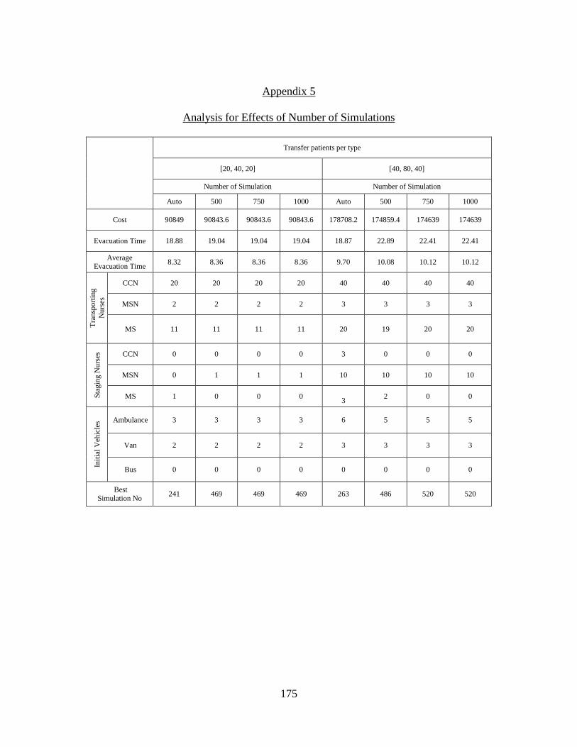
175

Appendix 5

Analysis for Effects of Number of Simulations

Transfer patients per type

[20, 40, 20] [40, 80, 40]

Number of Simulation Number of Simulation

Auto 500 750 1000 Auto 500 750 1000

Cost 90849 90843.6 90843.6 90843.6 178708.2 174859.4 174639 174639

Evacuation Time 18.88 19.04 19.04 19.04 18.87 22.89 22.41 22.41

Average Evacuation Time

8.32 8.36 8.36 8.36 9.70 10.08 10.12 10.12

Tra

nsp

ort

ing

Nu

rses

CCN 20 20 20 20 40 40 40 40

MSN 2 2 2 2 3 3 3 3

MS 11 11 11 11 20 19 20 20

Sta

gin

g N

urs

es

CCN 0 0 0 0 3 0 0 0

MSN 0 1 1 1 10 10 10 10

MS 1 0 0 0

3 2 0 0

Init

ial

Veh

icle

s Ambulance 3 3 3 3 6 5 5 5

Van 2 2 2 2 3 3 3 3

Bus 0 0 0 0 0 0 0 0

Best

Simulation No 241 469 469 469 263 486 520 520

176

Transfer patients per type

[60, 120, 60] [80, 160, 80]

Number of Simulation Number of Simulation

Auto 500 750 1000 Auto 500 750 1000

Cost 269382.2 260399 260399 258934.6 346976.2 342115.4 339759.4 338298.6

Evacuation Time 21.78 22.34 22.34 22.74 22.75 23.27 23.62 23.25

Average

Evacuation Time 7.5 10.91 10.91 11.08 11.38 11.66 12.02 11.95

Tra

nsp

ort

ing

Nu

rses

CCN 60 60 60 60 80 80 80 80

MSN 7 4 4 4 5 5 5 5

MS 30 28 28 29 39 38 38 37

Sta

gin

g N

urs

es

CCN 1 0 0 0 0 0 0 1

MSN 12 14 14 10 21 7 2 0

MS 6 3 3 1 4 5 4 5

Init

ial

Veh

icle

s

Ambulan

ce 8 8 8 8 10 10 10 10

Van 7 4 4 4 5 5 5 5

Bus 0 0 0 0 0 0 0 0

Best

Simulation No 256 451 451 955 184 332 740 935

177

Transfer patients per type

[100, 200, 100] [120, 240, 120]

Number of Simulation Number of Simulation

Auto 500 750 1000 Auto 500 750 1000

Cost 432930.4 432224 431468 431468 523547.4 512017.8 512017.8 509726

Evacuation Time 22.24 21.97 21.97 21.97 22.68 22.52 22.52 22.83

Average

Evacuation Time 10.72 10.68 10.68 10.68 10.97 10.99 10.99 11.18

Tra

nsp

ort

ing

Nu

rses

CCN 100 100 100 100 120 120 120 120

MSN 7 7 7 7 8 8 8 8

MS 49 48 48 48 56 56 56 58

Sta

gin

g N

urs

es

CCN 3 2 0 0 9 0 0 1

MSN 1 0 0 0 26 16 16 8

MS 13 16 16 16 6 5 5 3

Init

ial

Veh

icle

s Ambulance 13 13 13 13 15 15 15 15

Van 7 7 7 7 8 8 8 8

Bus 0 0 0 0 0 0 0 0

Best Simulation No

270 486 524 524 257 452 452 978

178

Appendix 6

Simulation Optimization Result Tables for Different Target Evacuation Times

Transfer patients per type: [20, 40, 20] & Bed/facility: [40, 80, 40]

Target Evacuation Time

≤ 12 ≤ 18 ≤ 24 ≤ 30 ≤ 36 ≤ 42

Cost 93300 91560.2 90843.6 94969 85654 87279

Evacuation Time 10.26 18.87 19.04 19.04 32.05 32.05

Average Evacuation Time 4.98 7.01 8.36 8.37 14.93 14.93

Transporting

Nurses

CCN 20 20 20 20 20 20

MSN 6 2 2 2 1 1

MS 9 10 11 11 11 11

Staging

Nurses

CCN 1 2 0 1 0 0

MSN 8 7 1 0 0 0

MS 6 4 0 0 0 0

Initial Vehicles

Ambulance 5 4 3 3 2 2

Van 0 2 2 2 1 1

Bus 2 0 0 0 0 0

Simulation No 418 454 469 244 194 317

Transfer patients per type: [40, 80, 40] & Bed/facility: [40, 80, 40]

Target Evacuation Time

≤ 12 ≤ 18 ≤ 24 ≤ 30 ≤ 36 ≤ 42

Cost 180560 175769.8 174859.4 180114 172082.4 173418.4

Evacuation Time 10.51 15.53 22.89 22.41 32.29 32.09

Average Evacuation Time 5.42 7.71 10.08 10.12 14.95 14.74

Transporting Nurses

CCN 40 40 40 40 40 40

MSN 8 4 3 3 2 2

MS 19 20 19 20 21 19

Staging

Nurses

CCN 2 0 0 0 0 0

MSN 17 5 10 10 6 4

MS 8 5 2 0 1 5

Initial

Vehicles

Ambulance 10 7 5 5 4 4

Van 4 4 3 3 2 2

Bus 1 0 0 0 0 0

Simulation No 491 429 486 259 438 463

179

Transfer patients per type: [60, 120, 60] & Bed/facility: [40, 80, 40]

Target Evacuation Time

≤ 12 ≤ 18 ≤ 24 ≤ 30 ≤ 36 ≤ 42

Cost 272662 262712.9 260399 257638.4 253790 251875.8

Evacuation Time 10.33 16.02 22.34 25.57 32.35 40.03

Average Evacuation Time 4.91 8.27 10.91 11.51 14.72 15.92

Transporting Nurses

CCN 60 60 60 60 60 60

MSN 16 9 4 4 3 3

MS 24 26 28 29 30 29

Staging Nurses

CCN 0 0 0 0 0 0

MSN 32 0 14 1 3 0

MS 8 10 3 3 3 2

Initial

Vehicles

Ambulance 15 10 8 7 6 5

Van 4 4 4 4 3 3

Bus 4 1 0 0 0 0

Simulation No 342 176 451 464 495 247

Transfer patients per type: [80, 160, 80] & Bed/facility: [40, 80, 40]

Target Evacuation Time

≤ 12 ≤ 18 ≤ 24 ≤ 30 ≤ 36 ≤ 42

Cost 350602.8 343190.4 342115.4 347603.5 342521.8 357781.4

Evacuation Time 10.64 16.67 23.27 27.21 32.83 39.61

Average Evacuation Time 5.42 8.61 11.66 12.85 14.80 12.75

Transporting Nurses

CCN 80 80 80 80 80 80

MSN 12 7 5 11 4 15

MS 35 38 38 37 37 37

Staging

Nurses

CCN 0 0 0 0 0 2

MSN 33 1 7 2 20 1

MS 8 9 5 2 6 5

Initial Vehicles

Ambulance 20 14 10 9 8 7

Van 12 7 5 3 4 2

Bus 0 0 0 1 0 2

Simulation No 431 361 332 320 401 485

180

Transfer patients per type: [100, 200, 100] & Bed/facility: [40, 80, 40]

Target Evacuation Time

≤ 12 ≤ 18 ≤ 24 ≤ 30 ≤ 36 ≤ 42

Cost 450198.8 440620.2 432224 418379.8 420241.4 420737.6

Evacuation Time 10.81 16.26 21.97 29.12 34.38 39.20

Average Evacuation Time 5.92 8.25 10.68 12.60 15.02 15.61

Transporting Nurses

CCN 100 100 100 100 100 100

MSN 23 16 7 6 5 5

MS 44 47 48 48 48 48

Staging

Nurses

CCN 1 0 2 0 0 0

MSN 6 14 0 1 1 1

MS 15 4 16 2 9 4

Initial

Vehicles

Ambulance 25 17 13 11 10 9

Van 7 6 7 6 5 5

Bus 4 2 0 0 0 0

Simulation No 404 271 486 443 468 317

Transfer patients per type: [120, 240, 120] & Bed/facility: [40, 80, 40]

Target Evacuation Time

≤ 12 ≤ 18 ≤ 24 ≤ 30 ≤ 36 ≤ 42

Cost 536053 518055.3 512017.8 498914.6 483915.6 527016.9

Evacuation Time 11.77 16.24 22.52 26.96 33.41 40.60

Average Evacuation Time 6.20 8.54 10.99 12.65 14.89 15.89

Transporting

Nurses

CCN 120 120 120 120 120 120

MSN 24 14 8 7 6 25

MS 57 55 56 56 55 55

Staging

Nurses

CCN 0 0 0 0 0 0

MSN 21 15 16 4 10 0

MS 12 5 5 3 5 2

Initial Vehicles

Ambulance 30 20 15 15 12 10

Van 8 9 8 7 6 2

Bus 4 1 0 0 0 3

Simulation No 405 481 452 492 456 316

181

Transfer patients per type: [20, 40, 20] & Bed/facility: [8, 16, 8]

Target Evacuation Time

≤ 12 ≤ 18 ≤ 24 ≤ 30 ≤ 36 ≤ 42

Cost 88590 91787 90843.6 95931.2 85654 87279

Evacuation Time 10.09 13.01 18.73 18.27 33.79 33.79

Average Evacuation Time 5.12 7.21 8.28 8.12 15.60 15.6

Transporting

Nurses

CCN 20 20 20 20 20 20

MSN 6 2 2 2 1 1

MS 5 11 11 11 11 11

Staging

Nurses

CCN 0 0 0 0 0 0

MSN 12 9 1 3 0 0

MS 7 2 0 0 0 0

Initial

Vehicles

Ambulance 5 4 3 3 2 2

Van 0 2 2 2 1 1

Bus 2 0 0 0 0 0

Simulation No 178 478 271 458 437 473

Transfer patients per type: [40, 80, 40] & Bed/facility: [8, 16, 8]

Target Evacuation Time

≤ 12 ≤ 18 ≤ 24 ≤ 30 ≤ 36 ≤ 42

Cost 178989 175435.6 173735.6 187035 173952.8 173310.4

Evacuation Time 10.98 15.70 22.36 19.16 32.38 32.62

Average Evacuation Time 5.9 8.04 10.27 9.81 12.47 15.07

Transporting Nurses

CCN 40 40 40 40 40 40

MSN 8 4 3 3 7 2

MS 18 21 21 21 17 21

Staging

Nurses

CCN 1 1 0 0 0 0

MSN 17 0 1 7 0 1

MS 7 2 1 0 4 0

Initial Vehicles

Ambulance 10 7 5 6 4 4

Van 2 4 3 3 1 2

Bus 2 0 0 0 1 1

Simulation No 479 471 398 347 390 474

182

Transfer patients per type: [60, 120, 60] & Bed/facility: [8, 16, 8]

Target Evacuation Time

≤ 12 ≤ 18 ≤ 24 ≤ 30 ≤ 36 ≤ 42

Cost 265300.2 261248.9 261520.6 270275.2 267775.2 268513.5

Evacuation Time 9.89 16.06 22.60 25.62 25.22 40.08

Average Evacuation Time 5.79 8.31 10.97 11.37 10.54 11.84

Transporting

Nurses

CCN 60 60 60 60 60 60

MSN 20 9 4 12 13 18

MS 21 25 30 23 24 24

Staging

Nurses

CCN 0 0 3 9 0 0

MSN 9 3 1 5 6 1

MS 15 10 5 6 14 3

Initial

Vehicles

Ambulance 16 10 8 7 7 5

Van 0 4 4 1 1 0

Bus 5 1 0 2 2 3

Simulation No 393 455 457 463 500 291

Transfer patients per type: [80, 160, 80] & Bed/facility: [8, 16, 8]

Target Evacuation Time

≤ 12 ≤ 18 ≤ 24 ≤ 30 ≤ 36 ≤ 42

Cost 355048.8 350446.9 350571.2 346840.8 347785.2 352862.4

Evacuation Time 10.19 15.85 23.77 26.64 32.27 39.29

Average Evacuation Time 5.49 8.14 11.64 12.14 12.46 12.73

Transporting

Nurses

CCN 80 80 80 80 80 80

MSN 21 11 14 5 14 15

MS 24 38 34 41 34 33

Staging Nurses

CCN 0 0 0 1 2 3

MSN 12 6 7 4 2 1

MS 10 6 5 4 5 8

Initial

Vehicles

Ambulance 20 14 10 9 8 7

Van 3 6 2 5 2 2

Bus 8 1 2 0 2 2

Simulation No 223 493 275 498 497 474

183

Transfer patients per type: [100, 200, 100] & Bed/facility: [8, 16, 8]

Target Evacuation Time

≤ 12 ≤ 18 ≤ 24 ≤ 30 ≤ 36 ≤ 42

Cost 445572 442569.9 435080.8 425032.7 424960.8 427163.7

Evacuation Time 10.42 15.74 22.80 29.06 33.54 38.79

Average Evacuation Time 5.56 7.80 11.21 11.96 15.03 16.78

Transporting

Nurses

CCN 100 100 100 100 100 100

MSN 22 18 10 11 5 11

MS 39 40 47 46 51 46

Staging Nurses

CCN 0 5 0 0 1 0

MSN 21 24 12 0 6 1

MS 17 11 3 3 0 3

Initial

Vehicles

Ambulance 25 18 13 11 10 9

Van 7 5 5 5 5 3

Bus 6 3 1 1 0 1

Simulation No 252 428 444 496 500 480

Transfer patients per type: [120, 240, 120] & Bed/facility: [8, 16, 8]

Target Evacuation Time

≤ 12 ≤ 18 ≤ 24 ≤ 30 ≤ 36 ≤ 42

Cost 528943.4 524477.8 521858 509800.2 494465.4 505437

Evacuation Time 11.51 17.06 22.47 27.80 32.48 40.97

Average Evacuation Time 6.16 8.88 9.82 12.83 13.22 18.87

Transporting

Nurses

CCN 120 120 120 120 120 120

MSN 27 10 20 23 7 5

MS 47 61 50 49 60 61

Staging

Nurses

CCN 0 0 0 0 0 0

MSN 19 29 6 2 9 6

MS 19 0 9 11 7 0

Initial Vehicles

Ambulance 30 20 15 14 12 10

Van 7 10 5 2 7 5

Bus 5 0 3 3 0 0

Simulation No 457 489 413 468 386 321

184

Appendix 7

Simulation Optimization Result Tables of Cases with Fixed Costs

for Different Target Evacuation Times

Transfer patients per type: [100, 200, 100] & Bed/facility: [40, 80, 40]

Target Evacuation Time

≤ 12 ≤ 18 ≤ 24 ≤ 30 ≤ 36 ≤ 42

Cost 515030 467040 436600 429560 425300 419220

Evacuation Time 11.35 17 22.59 28.99 33.04 39.32

Average Evacuation Time 6.1 8.84 10.89 12.53 14.85 15.52

Transporting

Nurses

CCN 100 100 100 100 100 100

MSN 24 8 7 6 5 5

MS 46 49 48 49 48 46

Staging

Nurses

CCN 1 0 0 0 0 1

MSN 22 28 1 0 14 3

MS 5 6 3 6 1 7

Initial

Vehicles

Ambulance 25 17 13 11 10 9

Van 4 8 7 6 5 5

Bus 5 0 0 0 0 0

Simulation No 495 445 467 500 450 447

Transfer patients per type: [100, 200, 100] & Bed/facility: [8,16, 8]

Target Evacuation Time

≤ 12 ≤ 18 ≤ 24 ≤ 30 ≤ 36 ≤ 42

Cost 497740 470330 449070 438540 426440 425280

Evacuation Time 11.48 15.89 23.88 29.36 34.21 34.35

Average Evacuation Time 6.41 8.28 11.46 12.42 15.34 15.33

Transporting

Nurses

CCN 100 100 100 100 100 100

MSN 22 18 20 16 5 5

MS 42 41 41 42 51 51

Staging

Nurses

CCN 0 9 1 0 0 1

MSN 0 12 2 1 0 0

MS 8 7 7 7 2 0

Initial

Vehicles

Ambulance 25 17 13 11 10 10

Van 7 5 2 3 5 5

Bus 4 3 3 2 0 0

Simulation No 410 271 366 470 432 489

185

Appendix 8

Simulation Optimization Result Tables for Different Evacuation Start Times

Before Landfall

Transfer patients per type: [20, 40, 20] & Bed/facility: [40, 80, 40]

Evacuation Start Before Landfall

30 36 42 48

Cost 78702 83124.6 85557 90843.6

Evacuation Time 20.83 16.77 20.99 19.04

Average Evacuation Time 10.98 8.65 8.62 8.36

Transporting

Nurses

CCN 20 20 20 20

MSN 2 2 2 2

MS 11 11 11 11

Staging

Nurses

CCN 0 0 0 0

MSN 0 0 1 1

MS 0 1 0 0

Initial

Vehicles

Ambulance 4 4 3 3

Van 2 2 2 2

Bus 0 0 0 0

Simulation No 306 329 405 180

Transfer patients per type: [40, 80, 40] & Bed/facility: [40, 80, 40]

Evacuation Start Before Landfall

30 36 42 48

Cost 161386.2 164022.4 165172.8 1714506

Evacuation Time 22.75 21.97 21.22 22.52

Average Evacuation Time 12.41 9.75 10.23 10.39

Transporting

Nurses

CCN 40 40 40 40

MSN 11 7 3 3

MS 20 18 21 19

Staging

Nurses

CCN 0 1 0 0

MSN 3 3 0 4

MS 3 4 1 1

Initial

Vehicles

Ambulance 7 7 6 5

Van 0 2 3 3

Bus 2 1 0 0

Simulation No 442 497 433 277

186

Transfer patients per type: [60, 120, 60] & Bed/facility: [40, 80, 40]

Evacuation Start Before Landfall

30 36 42 48

Cost 227006 246345.6 258103.2 259934.6

Evacuation Time 23.29 22.02 20.45 22.74

Average Evacuation Time 11.64 9.49 8.33 11.08

Transporting Nurses

CCN 60 60 60 60

MSN 6 9 11 4

MS 29 29 28 29

Staging

Nurses

CCN 2 3 0 0

MSN 0 10 3 10

MS 2 5 2 1

Initial Vehicles

Ambulance 10 10 9 8

Van 6 4 3 4

Bus 0 1 2 0

Simulation No 487 495 478 326

Transfer patients per type: [80, 160, 80] & Bed/facility: [40, 80, 40]

Evacuation Start Before Landfall

30 36 42 48

Cost 302836.2 315099.8 325881.8 342115.4

Evacuation Time 23.75 23.11 22.38 23.27

Average Evacuation Time 12.36 10.34 10.65 11.66

Transporting Nurses

CCN 80 80 80 80

MSN 7 7 6 5

MS 37 39 39 38

Staging Nurses

CCN 0 0 0 0

MSN 2 0 0 7

MS 10 4 1 5

Initial Vehicles

Ambulance 14 14 12 10

Van 7 7 6 5

Bus 0 0 0 0

Simulation No 499 401 389 400

187

Transfer patients per type: [100, 200, 100] & Bed/facility: [40, 80, 40]

Evacuation Start Before Landfall

30 36 42 48

Cost 378628 399985 414135 426759.2

Evacuation Time 23.96 23.35 20.54 22.6

Average Evacuation Time 11.99 10.52 9.00 10.9

Transporting Nurses

CCN 100 100 100 100

MSN 13 13 9 7

MS 48 46 46 49

Staging Nurses

CCN 1 1 0 0

MSN 0 8 6 4

MS 1 3 8 0

Initial

Vehicles

Ambulance 17 17 15 13

Van 8 7 9 7

Bus 1 1 0 0

Simulation No 370 416 490 467

Transfer patients per type: [120, 240, 120] & Bed/facility: [40, 80, 40]

Evacuation Start Before Landfall

30 36 42 48

Cost 447028.4 469221.2 499113.8 507696

Evacuation Time 23.56 23.29 21.47 22.96

Average Evacuation Time 12.31 11.00 10.15 11.31

Transporting

Nurses

CCN 120 120 120 120

MSN 11 10 9 8

MS 58 56 57 55

Staging

Nurses

CCN 0 0 0 0

MSN 5 0 27 3

MS 3 9 7 6

Initial

Vehicles

Ambulance 20 20 18 15

Van 11 10 9 8

Bus 0 0 0 0

Simulation No 288 461 491 462

188

Transfer patients per type: [20, 40, 20] & Bed/facility: [8, 16, 8]

Evacuation Start Before Landfall

30 36 42 48

Cost 78462 85084.8 85551.6 90843.6

Evacuation Time 20.97 16.23 21.42 18.73

Average Evacuation Time 11.01 7.17 8.72 8.28

Transporting Nurses

CCN 20 20 20 20

MSN 2 4 2 2

MS 11 9 11 11

Staging Nurses

CCN 0 0 0 0

MSN 0 8 0 1

MS 0 2 1 0

Initial Vehicles

Ambulance 4 4 3 3

Van 2 1 2 2

Bus 0 1 0 0

Simulation No 416 408 393 216

Transfer patients per type: [40, 80, 40] & Bed/facility: [8, 16, 8]

Evacuation Start Before Landfall

30 36 42 48

Cost 157110.6 164884.2 166249.8 174113.6

Evacuation Time 23.18 22.05 21.02 22.36

Average Evacuation Time 12.38 7.96 10.52 10.27

Transporting

Nurses

CCN 40 40 40 40

MSN 12 12 3 3

MS 16 15 21 21

Staging

Nurses

CCN 0 0 0 1

MSN 2 1 0 1

MS 4 3 1 1

Initial

Vehicles

Ambulance 7 7 6 5

Van 0 0 3 3

Bus 2 3 0 0

Simulation No 386 420 393 426

189

Transfer patients per type: [60, 120, 60] & Bed/facility: [8, 16, 8]

Evacuation Start Before Landfall

30 36 42 48

Cost 227219.4 240588.2 251893.8 261520.6

Evacuation Time 23.34 23.70 21.55 22.60

Average Evacuation Time 11.77 10.50 9.82 10.97

Transporting

Nurses

CCN 60 60 60 60

MSN 9 12 11 4

MS 28 26 25 30

Staging Nurses

CCN 0 0 0 3

MSN 5 1 2 1

MS 2 5 4 5

Initial Vehicles

Ambulance 10 10 9 8

Van 4 2 2 4

Bus 1 2 2 0

Simulation No 425 496 435 457

Transfer patients per type: [80, 160, 80] & Bed/facility: [8, 16, 8]

Evacuation Start Before Landfall

30 36 42 48

Cost 305676.4 322376 333156.8 348792.2

Evacuation Time 23.52 22.72 21.61 23.58

Average Evacuation Time 11.75 10.18 10.16 11.66

Transporting

Nurses

CCN 80 80 80 80

MSN 13 14 15 14

MS 34 36 31 35

Staging Nurses

CCN 0 2 0 0

MSN 3 0 1 2

MS 6 4 9 4

Initial Vehicles

Ambulance 14 14 12 10

Van 5 4 3 2

Bus 2 2 2 2

Simulation No 409 454 407 349

190

Transfer patients per type: [100, 200, 100] & Bed/facility: [8, 16, 8]

Evacuation Start Before Landfall

30 36 42 48

Cost 380552 400882.4 414682.6 435297.6

Evacuation Time 23.54 22.17 21.80 22.18

Average Evacuation Time 12.31 9.62 10.40 9.84

Transporting

Nurses

CCN 100 100 100 100

MSN 19 20 12 8

MS 43 40 46 50

Staging Nurses

CCN 1 0 0 0

MSN 1 7 0 0

MS 7 9 6 9

Initial Vehicles

Ambulance 17 17 15 13

Van 4 5 6 8

Bus 3 3 1 0

Simulation No 450 284 444 478

Transfer patients per type: [120, 240, 120] & Bed/facility: [8, 16, 8]

Evacuation Start Before Landfall

30 36 42 48

Cost 463680.4 489672.8 498410.8 531397.2

Evacuation Time 23.38 22.38 22.52 22.89

Average Evacuation Time 11.64 10.15 10.47 10.50

Transporting

Nurses

CCN 120 120 120 120

MSN 30 32 17 30

MS 47 44 55 45

Staging Nurses

CCN 3 0 2 0

MSN 3 6 0 7

MS 13 21 5 12

Initial Vehicles

Ambulance 20 20 18 15

Van 2 1 6 1

Bus 6 6 2 5

Simulation No 385 380 447 482

191

Appendix 9

Simulation Optimization Result Tables of Cases with Fixed Costs

for Different Evacuation Start Times Before Landfall

Transfer patients per type: [100, 200, 100] & Bed/facility: [40, 80, 40]

Evacuation Start Before Landfall

30 36 42 48

Cost 451720 451520 445880 439860

Evacuation Time 23.64 23.46 21.80 22.37

Average Evacuation Time 12.49 10.68 10.28 10.91

Transporting

Nurses

CCN 100 100 100 100

MSN 9 9 8 7

MS 44 46 48 49

Staging Nurses

CCN 1 0 6 5

MSN 4 2 0 1

MS 5 3 1 5

Initial Vehicles

Ambulance 17 17 15 13

Van 9 9 8 7

Bus 0 0 0 0

Simulation No 236 479 496 474

Transfer patients per type: [100, 200, 100] & Bed/facility: [8, 16, 8]

Evacuation Start Before Landfall

30 36 42 48

Cost 461530 454400 454290 451090

Evacuation Time 23.39 23.32 22.48 23.01

Average Evacuation Time 11.60 10.44 10.47 11.33

Transporting

Nurses

CCN 100 100 100 100

MSN 20 9 11 22

MS 40 48 47 40

Staging Nurses

CCN 0 0 1 0

MSN 1 2 13 8

MS 9 2 2 7

Initial Vehicles

Ambulance 17 17 15 13

Van 5 9 6 2

Bus 3 0 1 3

Simulation No 268 466 345 315

192

Appendix 10

Heuristic Result Tables of [DDM]

Heuristic Result Tables of [DDM] for Single-Product Delivery

Product 1

Number of

customers 3 5 10 15 20

Demand distribution

DD1 DD2 DD1 DD2 DD1 DD2 DD1 DD2 DD1 DD2

Profit 27566.5 49989.5 47681.4 82033.9 99952.25 171953.75 146986.95 251098.45 201585.15 343050.65

Budget 188086.5 309403.5 311935.5 516653 613682 1022980.5 941363 1553781.5 1241353 2058367.5

Unit-volume 1800 3000 3011.4 5011.4 5934.2 9934.2 9116 15116 12040.9 20040.9

Veh

icle

Type 1 0 0 0 0.15 0.1 0 0 0.05 0 0

Type 2 4.9 5.65 6.65 8.75 11.75 16.15 16.65 22.6 20.05 28.55

Mat

eria

l

Han

dle

r 1st Shift 1.5 2.05 2.1 3.7 4 6.95 6.25 10.95 8.7 14.55

2nd Shift 1.75 2.1 2.1 3.7 4 6.95 6.25 10.95 8.7 14.55

Product 2

Number of

customers 3 5 10 15 20

Demand

distribution DD1 DD2 DD1 DD2 DD1 DD2 DD1 DD2 DD1 DD2

Profit 28609 50646.5 48561.9 88144.9 106622.75 183233.75 156901.95 268531.45 214482.15 364971.65

Budget 133044 218746.5 220713 360200 428985.5 713674.5 657968 1082868.5 867229 1435219.5

Unit-volume 900 1500 1505.7 2505.7 2967.1 4967.1 4558 7558 6020.45 10020.45

Veh

icle

Type 1 0 0 0.1 0.15 0 0.1 0.05 0.05 0 0

Type 2 4.2 5.55 6.4 5.65 8.45 10.3 11.8 14.15 14.35 17.95

Mat

eria

l

Han

dle

r 1st Shift 1 1 1.1 2 2 3.65 3 5 4.05 7

2nd Shift 1 1.1 1.1 2 2 3.65 3 5 4.05 7

193

Heuristic Result Tables of [DDM] for Two-Product Delivery

Same Demand Distributions

Number of

customers 3 5 10 15 20

Demand distribution

DD1 DD2 DD1 DD2 DD1 DD2 DD1 DD2 DD1 DD2

Profit 62024.2 103552.7 102959.75 177971.75 207687.15 354116.15 316742.75 538354.75 422785.85 718410.35

Budget 315511 525482.5 521541.5 867829.5 1055707 1747758 1576707 2615775 2088385 3473371

Unit-volume 2682.45 4482.45 4448.65 7448.65 9048.50 15048.5 13535.55 22535.55 17942.75 29942.75

Veh

icle

Type 1 0 0.05 0 0 0.15 0.15 0 0.2 0.3 0.05

Type 2 6.15 9.35 10.2 13.4 17.8 23 24.2 33.65 29.95 42.5

Mat

eria

l

Han

dle

r 1st Shift 2 3 3.05 5.05 6.2 10.95 9.85 16.35 13.1 21.95

2nd Shift 2 3 3.05 5.05 6.2 10.95 9.85 16.35 13.1 21.95

Different Demand Distributions

Number of

customers 3 5 10 15 20

Demand

distribution MDD1 MDD2 MDD1 MDD2 MDD1 MDD2 MDD1 MDD2 MDD1 MDD2

Profit 82833.2 82515.7 140255.75 141944.75 284988.65 275910.15 428584.25 426222.25 574971.85 565438.85

Budget 401772 439499.5 663185.5 724916.5 1339335.5 1465034 2003035.5 2189737.5 2656389.5 2906152.5

Unit-volume 3282.45 3882.45 5448.65 6448.65 11048.5 13048.5 16535.55 19535.55 21942.75 25942.75

Veh

icle

Type 1 0.1 0.05 0.2 0.05 0.2 0.1 0.2 0.2 0.05 0.25

Type 2 7.25 7.8 10.5 11.9 18.85 22.45 27.4 30.9 34.25 39.25

Mat

eria

l

Han

dle

r 1st Shift 2.5 3 3.95 4.4 7.95 9.2 11.95 14.1 16 19

2nd Shift 2.5 3 3.95 4.4 7.95 9.2 11.95 14.1 16 19

194

Appendix 11

Optimal Result Tables of [RSCSDDM]

Optimal Result Tables of [RSCSDDM] for Single-Product Delivery

Demand Distribution = DD1

Product type Product 1 Product 2

Number of customers 3 5 3 5 10

Storage (volume) restriction

25% 50% 25% 50% 25% 50% 25% 50% 50%

Unit-volume 1181.9 665.3 2058.71 1338 590.95 332.65 1037.9 669.05 1466.14

Number of

selected customers 1.95 1.05 3.29 2.2 1.95 1.05 3.4 2.2 4.86

Profit 22354.35 13805.05 38135.94 27608.05 23546.35 14675.55 41552.25 28952.25 69163.86

Budget 121662 68818 211204.71 137563 85013 47988.5 148601.5 96088 209617.14

Veh

icle

Type 1 1.2 0.45 1.59 0.9 0.4 1 1.45 0.9 2

Type 2 0.8 0.75 1.47 1.15 0.75 0 0.55 0.55 1

Mat

eria

l

Han

dle

r 1st Shift 2 1.9 2 2 2 1.7 1.95 2 2

2nd Shift 1.7 0.75 1.94 1.7 0.7 0.1 1.25 0.7 1

Demand Distribution = DD2

Product type Product 1 Product 2

Number of customers 3 5 3 5 10

Storage (volume)

restriction 25% 50% 25% 50% 25% 50% 25% 50% 50%

Unit-volume 1999.9 1052.8 3071.67 2102.2 999.95 526.4 1653.35 1054.55 2297

Number of

selected customers 2 1 3 2.1 2 1 3.3 2.1 4

Profit 38536.7 22295.4 64602.5 45217.3 40538.2 23549.4 67589.35 47336.2 125516

Budget 205118 108425 314458.33 215528.5 143119.5 75528.5 235919 150860.5 327170

Veh

icle

Type 1 1.75 0.85 1 1.1 1.55 0.25 0.7 1.05 1

Type 2 1.25 1.05 3.17 1.85 0.45 0.75 1.7 0.95 2

Mat

eria

l

Han

dle

r 1st Shift 2 2 2.17 2 1.95 1.75 2 1.9 2

2nd Shift 2 0.55 2 1.95 0.75 0.4 1.75 0.65 2

195

Optimal Result Tables of [RSCSDDM] for Two-Product Delivery

Same Demand Distributions

Demand Distribution DD1 DD2

Number of customers 3 5 3 5

Storage (volume)

restriction 25% 50% 25% 50% 25% 50% 50%

Unit-volume 1841.1 940.9 2784.4 1948.35 3051.3 1511.95 3056.95

Number of

selected customers 2 1 3 2.15 2 1 2

Profit 47384.55 26459.45 74064.1 52711 80185.6 43657 86116.5

Budget 214459.5 110263.5 321323 226286.5 354096 176271.5 353395

Veh

icle

Type 1 1.6 1.2 1.4 1.5 0.9 0.6 1.1

Type 2 1.25 0.6 2.6 1.5 3.3 1.55 3.2

Mat

eria

l

Han

dle

r 1st Shift 2 2 2 2 2.1 2 2.15

2nd Shift 2 0.65 2 1.9 2.15 1.65 2

Different Demand Distributions

Product type MDD1 MDD2

Number of customers 3 5 3 5

Storage (volume)

restriction 25% 50% 25% 50% 25% 50% 50%

Unit-volume 2238.35 1135.05 3311 2282.05 2657.5 1338.25 2670.3

Number of

selected customers 2 1 3 2 2 1 2

Profit 63958.15 35178.85 91271 70351.9 64855.65 34993.45 69538.55

Budget 271386 138261.5 399500 274889 297878 150790 298238.5

Veh

icle

Type 1 1.75 0.9 2 1.15 1.3 0.55 1.2

Type 2 1.55 1.1 3 2 2.45 1.55 2.55

Mat

eria

l

Han

dle

r 1st Shift 2 2 2.5 2 2 2 2

2nd Shift 2 0.85 2 2 2 1.05 2

196

Appendix 12

Heuristic Result Tables of [RSCSDDM]

Heuristic Result Tables of [RSCSDDM] for Only Product 1 Delivery

Demand Distribution = DD1

Number of

customers 3 5 10 15 20

Storage (volume) restriction

25% 50% 25% 50% 25% 50% 25% 50% 25% 50%

Unit-volume 1199.33 663.6 2075.9 1346.22 4311.8 2887.7 6761.3 4486 8977.7 5960.8

Number of selected customers

1.94 1.07 3.4 2.22 7.15 5 11.1 7.45 14.85 9.8

Profit 19743.39 11275.8 37132.45 23693.78 80278.3 60467.45 122727.5 91328.5 171251.4 126725.6

Budget 126513.33 70882 215307.5 142718.89 448455.5 299636 699195.5 465245.5 926895.5 616858

Veh

icle

Type 1 0 0 0.15 0.06 0 0 0 0 0 0

Type 2 3.89 2.47 4.35 4.94 10.3 6.8 12.8 9.9 16.4 12.4

Mat

eria

l

Han

dle

r 1st Shift 1 1 2 1 3 2 5 3 6 4

2nd Shift 1 1 1.95 1 3 2 5 3 6 4

Demand Distribution = DD2

Number of

customers 3 5 10 15 20

Storage (volume)

restriction 25% 50% 25% 50% 25% 50% 25% 50% 25% 50%

Unit-volume 2000.89 1052.8 3300.4 2102.84 7073.1 4860.4 11206.9 7312.4 14858.2 9867.7

Number of

selected customers 2 1 3.3 2.11 7.1 4.95 11.05 7.25 14.8 9.85

Profit 38316.06 19591.9 60927 44227.37 139444.3 103311.05 210173.8 153566.45 290201.85 213812.35

Budget 207205.56 111070 341213.5 217583.68 729850.5 503147.5 1153004.5 754446.5 1527551.5 1016785

Veh

icle

Type 1 0 0 0 0.05 0.05 0 0 0 0 0

Type 2 3.89 3.15 6.5 4.05 12.55 10.15 17.1 13.1 22.2 16.55

Mat

eria

l

Han

dle

r 1st Shift 2 1 2.45 1.95 5 3.15 8 5 10.8 7

2nd Shift 2 1 2.45 2 5 3.15 8 5 10.8 7

197

Heuristic Result Tables of [RSCSDDM] for Only Product 2 Delivery

Demand Distribution = DD1

Number of

customers 3 5 10 15 20

Storage (volume) restriction

25% 50% 25% 50% 25% 50% 25% 50% 25% 50%

Unit-volume 590.95 336.42 1037.95 669.05 2155.9 1443.85 3382.4 2249.55 4497.3 2980.4

Number of selected customers

1.95 1.05 3.4 2.2 7.15 5 11.1 7.5 14.9 9.8

Profit 20580.85 13373.53 36957.95 26148.75 87752.8 61065.95 131760.15 98411.35 180816.6 132755.6

Budget 87978.5 50198.42 153205 98891.5 311627 212406.5 487573 324520.5 649257 432004

Veh

icle

Type 1 0 0.05 0.1 0 0 0 0.05 0 0.05 0

Type 2 3.1 2.11 4.8 3.15 6 6.55 7.9 5.8 11.9 9.5

Mat

eria

l

Han

dle

r 1st Shift 1 1 1 1 2 1 3 2 3 2

2nd Shift 0.95 0 1 1 2 1 3 2 3 2

Demand Distribution = DD2

Number of

customers 3 5 10 15 20

Storage (volume)

restriction 25% 50% 25% 50% 25% 50% 25% 50% 25% 50%

Unit-volume 999.95 526.4 1650.2 1051.1 3563.4 2430.85 5603.45 3656.2 7429.1 4940.05

Number of

selected customers 2 1 3.3 2.1 7.15 4.95 11.05 7.25 14.8 9.85

Profit 36487.2 21017.9 63471 43798.3 148224.4 111556.15 222293.8 162768.95 307537.35 226220.85

Budget 147170.5 78060 239657.5 153881.5 512712 349184 804677.5 525872 1064470 709350.5

Veh

icle

Type 1 0.25 0.15 0 0 0 0 0 0 0 0.05

Type 2 4.2 2.3 5.25 3.9 7.85 5.35 11.2 8 13.75 9.95

Mat

eria

l

Han

dle

r 1st Shift 1 1 1.35 1 3 2 4 3 5 3.65

2nd Shift 1 0.9 1.35 1 3 2 4 3 5 3.65

198

Heuristic Result Tables of [RSCSDDM] for Two-Product Delivery with SDD

Demand Distribution = DD1

Number of

customers 3 5 10 15 20

Storage (volume) restriction

25% 50% 25% 50% 25% 50% 25% 50% 25% 50%

Unit-volume 1841.1 940.9 2896.95 1948.35 6561.3 4422.9 10025.65 6703.5 13378.95 8925.2

Number of selected customers

2 1 3.2 2.15 7.2 4.95 11.15 7.5 14.95 10

Profit 44226.05 23696.95 72491.85 49841 161335.45 113653.9 251250.25 180931.7 342984.25 239741.85

Budget 217618 113026 339422.5 229254 770503.5 522642 1175881.5 787051.5 1563068 1051835.5

Veh

icle

Type 1 0 0.2 0.15 0 0 0 0.05 0 0.05 0

Type 2 4.65 2.85 7.05 4.5 14.65 11.5 22.8 14.25 24.1 21.65

Mat

eria

l

Han

dle

r 1st Shift 1.75 1 2.05 1.85 4.6 3 7 4.95 9.9 6

2nd Shift 1.8 1 2.05 1.9 4.6 3 7 4.95 9.9 6

Demand Distribution = DD2

Number of

customers 3 5 10 15 20

Storage (volume)

restriction 25% 50% 25% 50% 25% 50% 25% 50% 25% 50%

Unit-volume 3051.3 1511.95 4717.35 3056.95 10718.65 7379.55 16557.55 10951.55 22310.7 14865.8

Number of

selected customers 2 1 3.15 2 7.1 4.95 10.95 7.25 14.95 9.95

Profit 77813.6 40717.5 120634.55 83767.5 272965.9 195519.65 431988.2 300354.95 574544.6 411444.3

Budget 356468 179211 550972.5 355758.5 1248232 863294 1926241.5 1276843.5 2600480.5 1735378.5

Veh

icle

Type 1 0 0.1 0.15 0 0.05 0.05 0.05 0.05 0.05 0

Type 2 5.9 3.9 9.5 5.7 18.1 14.95 27.35 19.35 39 26.5

Mat

eria

l

Han

dle

r 1st Shift 2 1 3.2 2.1 7.8 4.95 12 7.95 16 10.95

2nd Shift 2 1.3 3.2 2.15 7.8 4.95 12 7.95 16 10.95

199

Heuristic Result Tables of [RSCSDDM] for Two-Product Delivery with DDD

Demand Distribution = MDD1

Number of

customers 3 5 10 15 20

Storage (volume) restriction

25% 50% 25% 50% 25% 50% 25% 50% 25% 50%

Unit-volume 2238.35 1135.05 3467.8 2282.05 8004.25 5388.5 12212.65 8100.8 16318.35 10920.4

Number of selected customers

2 1 3.15 2.05 7.2 4.95 11.1 7.45 14.9 10

Profit 62381.65 32680.35 96360.9 68354.4 220902.8 157617.5 344142.85 242787.9 462484.65 332149.6

Budget 272962.5 140760 422159 276886.5 974731.5 658699.5 1484593 989375.5 1984595.5 1331516

Veh

icle

Type 1 0 0.05 0 0.05 0.1 0 0.1 0.1 0.2 0.05

Type 2 4 3 7.45 4.4 16.65 11.4 23 16.95 29.65 21.3

Mat

eria

l

Han

dle

r 1st Shift 2 1 2.65 2 5.65 4 9 5.9 11.95 8

2nd Shift 2 1 2.7 2 5.65 4 9 5.9 11.95 8

Demand Distribution = MDD2

Number of

customers 3 5 10 15 20

Storage (volume)

restriction 25% 50% 25% 50% 25% 50% 25% 50% 25% 50%

Unit-volume 2657.5 1346.35 4089.95 2670.3 9344.9 6392.45 14411.6 9498.65 19342.65 12887.8

Number of

selected customers 2 1 3.15 2 7.15 4.95 11 7.25 14.95 9.95

Profit 62671.15 32245.25 95636.6 67108.55 213908.8 155107.4 340966.45 239258.95 451235.1 325077.4

Budget 300062.5 154348.5 462901.5 300668.5 1053097 722598 1623005 1071791 2180155.5 1453893.5

Veh

icle

Type 1 0 0.05 0.2 0.1 0 0.05 0.1 0.1 0.15 0.1

Type 2 5.1 3.5 9.2 5.3 17.85 14.05 27.1 19.25 36.65 25.4

Mat

eria

l

Han

dle

r 1st Shift 2 1 3 2 6.75 4 10 6.9 14 9

2nd Shift 2 1 3 2 6.75 4 10 6.9 14 9

200

Appendix 13

Integrality and Optimality Gaps of Cases with Restricted Storage Space

Integrality Gap

1 Product Type 2 product Type

Product 1 Product 2 SDD DDD

DD1 DD2 DD1 DD2 DD1 DD2 MDD1 MDD2

Nu

mb

er o

f cu

sto

mer

s

3

25% 17.40 5.45 15.75 12.13 7.74 3.19 2.72 3.55

50% 22.33 15.22 13.19 13.70 12.27 7.46 8.07 8.62

5 25% 6.39 5.01 13.01 6.90 6.40 N/A 4.46 N/A

50% 19.05 4.60 10.81 8.36 5.77 2.88 3.00 3.61

10

25% N/A N/A N/A N/A N/A N/A N/A N/A

50% N/A N/A 9.56 2.34 N/A N/A N/A N/A

Optimality Gap

1 Product Type 2 product Type

Product 1 Product 2 SDD DDD

DD1 DD2 DD1 DD2 DD1 DD2 MDD1 MDD2

Nu

mb

er o

f cu

sto

mer

s

3 25% 21.99 7.13 20.73 14.69 9.37 3.77 3.63 4.34

50% 29.91 19.16 18.59 17.09 15.38 9.06 10.25 10.62

5 25% 8.32 6.31 15.70 8.17 6.76 4.96 5.43 7.17

50% 22.27 5.89 14.38 10.28 7.17 3.48 3.81 4.35

10

25% 9.53 4.78 5.72 3.93 6.66 3.40 5.03 5.03

50% 7.25 6.06 11.57 3.02 8.30 4.65 5.03 5.77

15 25% 6.45 3.38 4.91 3.43 6.82 3.08 4.10 4.63

50% 7.22 4.40 4.63 3.56 5.64 3.46 4.78 5.23

20 25% 5.20 2.84 5.26 2.49 4.17 3.64 3.83 5.10

50% 5.84 3.66 6.09 2.92 6.98 3.59 4.06 4.90

201

Appendix 14

Optimal Result Tables of [RBCSDDM]

Optimal Result Tables of [RBCSDDM] for Single-Product Delivery

Demand Distribution = DD1

Product 1 Product 2

Number of

customers 3 5 10 3 5 10

Budget restriction 25% 50% 25% 50% 50% 50% 25% 50% 25% 50%

Budget 121662 68818 212404.71 138705 303070 87218 47988.5 151117.37 96875. 212920

Number of

selected customers 1.95 1.05 3.35 2.25 5 2 1.05 3.47 2.25 4.67

Profit 22354.35 13805.05 39765.47 27981.95 73786.00 23943.95 14675.55 42660.63 29350.65 71813.67

Unit-volume 1181.90 665.3 2070.47 1349.00 2960.00 606.35 332.65 1055.53 674.55 1490.00

Veh

icle

Type 1 1.20 0.45 1.53 0.95 1.00 0.45 1.00 1.42 0.90 2.33

Type 2 0.80 0.75 1.53 1.20 3.00 0.75 0.00 0.58 0.55 0.67

Mat

eria

l

Han

dle

r 1st Shift 2.00 1.9 2 2.00 2.00 2 1.70 1.95 1.95 2.00

2nd Shift 1.70 0.75 1.94 1.55 2.00 0.7 0.10 1.37 0.80 1.00

Demand Distribution = DD2

Product 1 Product 2

Number of

customers 3 5 10 3 5 10

Budget restriction 25% 50% 25% 50% 50% 50% 25% 50% 25% 50%

Budget 207548 108366.5 319618.57 215528.5

No

Solution

144792.5 75528.5 236447 150830.5 327170

Number of

selected customers 2 1 3 2.1 2 1 3.30 2.05 4

Profit 39206.35 22295.40 65900.86 45217.30 41250.85 23549.4 67680.35 47336.20 125516.00

Unit-volume 2023.7 1052.80 3121.43 2102.20 1011.85 526.4 1656.65 1054.55 2297.00

Veh

icle

Type 1 1.65 0.85 1.14 1.10 1.35 0.25 0.75 1.05 1.00

Type 2 1.35 1.05 3.14 1.85 0.65 0.75 1.65 0.95 2

Mat

eria

l

Han

dle

r 1st Shift 2 2.00 2.29 2.00 1.95 1.75 2.00 1.90 2

2nd Shift 2 0.55 2.00 1.95 0.65 0.4 1.80 0.65 2

202

Optimal Result Tables of [RBCSDDM] for Two-Product Delivery

Same Demand Distributions

Demand Distribution DD1 DD2

Number of customers 3 5 3 5

Budget restriction 25% 50% 25% 50% 25% 50% 50%

Budget 213487.5 110263.5 321078.75 222848.5 354096 176271.5 353409.5

Number of

selected customers 2 1 3 2.05 2 1 2

Profit 47239.85 26459.45 72377.25 52516.95 80185.6 43657 86116.5

Unit-volume 1834.7 940.9 2785 1920.35 3051.3 1509.25 3056.95

Veh

icle

Type 1 1.55 1.2 1.38 1.45 0.9 0.6 1.1

Type 2 1.3 0.6 2.63 1.5 3.3 1.55 3.2

Mat

eria

l

Han

dle

r 1st Shift 2 2 2 2 2.1 2 2.15

2nd Shift 2 0.65 2 1.9 2.15 1.65 2

Different Demand Distributions

Product type MDD1 MDD2

Number of customers 3 5 3 5

Budget restriction 25% 50% 25% 50% 25% 50% 50%

Budget 271314 138261.5 416990 274889 297878 150790 298238.5

Number of

selected customers 2 1 3 2.05 2 1 2

Profit 64156.2 35178.85 80649 70351.9 64855.65 34993.45 69538.55

Unit-volume 2239.35 1135.05 3441 2282.05 2657.5 1338.25 2670.3

Veh

icle

Type 1 1.75 0.9 2 1.15 1.3 0.55 1.2

Type 2 1.55 1.1 3 2 2.45 1.55 2.55

Mat

eria

l

Han

dle

r 1st Shift 2 2 3 2 2 2 2

2nd Shift 2 0.85 2 2 2 1.05 2

203

Appendix 15

Heuristic Result Tables of [RBCSDDM]

Heuristic Result Tables of [RBCSDDM] for Only Product 1 Delivery

Demand Distribution = DD1

Number of

customers 3 5 10 15 20

Budget restriction 25% 50% 25% 50% 25% 50% 25% 50% 25% 50%

Budget 126546.67 71450 217915 144219.44 451181.5 301640 705102.5 469472 934728.5 621537

Number of

selected customers 1.94 1.06 3.45 2.28 7.25 5 11.15 7.6 15 9.9

Profit 19710.06 11852.31 37583.35 23877.56 81413.7 61561.45 123931.9 91649.95 171870.9 127478.15

Unit-volume 1199.33 671.38 2100.40 1358.44 4343.2 2911.7 6818.9 4526 9051.5 6008.4

Veh

icle

Type 1 0 0 0.05 0 0 0 0 0 0 0

Type 2 3.94 2.31 4.5 5.11 10 6.4 12.85 10.05 16.7 12.2

Mat

eria

l

Han

dle

r 1st Shift 1 1 2 1 3 2 5 3 6 4

2nd Shift 1 1 1.95 1 3 2 5 3 6 4

Demand Distribution = DD2

Number of

customers 3 5 10 15 20

Budget restriction 25% 50% 25% 50% 25% 50% 25% 50% 25% 50%

Budget 210161.67 111172.5 342080.5 222061.05 738426.5 504919.5 1154311 758189.5 1533295.5 1024473.5

Number of

selected customers 2 1 3.3 2.16 7.2 4.95 11.05 7.35 14.85 9.95

Profit 38804 19489.4 60813 44465.7 139501.25 104770.25 210856.2 153992 291129.3 215223.2

Unit-volume 2027.33 1052.8 3307 2144.95 7152.5 4887.6 11223.4 7345.9 14912.1 9944.3

Veh

icle

Type 1 0.11 0.05 0 0 0 0 0 0 0 0

Type 2 4.06 3.15 6.65 4.26 13.05 9.35 16.95 13.3 22.4 16.5

Mat

eria

l

Han

dle

r 1st Shift 2 1 2.45 2 5 3.35 8 5 10.9 7

2nd Shift 2 1 2.45 2 5 3.35 8 5 10.9 7

204

Heuristic Result Tables of [RBCSDDM] for Only Product 2 Delivery

Demand Distribution = DD1

Number of

customers 3 5 10 15 20

Budget restriction 25% 50% 25% 50% 25% 50% 25% 50% 25% 50%

Budget 90743.5 51377.5 157659.5 100721.5 313686.5 216559 494647 328959 655581 437293.5

Number of

selected customers 2 1.1 3.55 2.3 7.3 5 11.25 7.55 15 10

Profit 20418.45 13197.15 37991.3 26565.95 89154.1 62414.3 133714.6 99225.75 181838.15 135148.7

Unit-volume 606.35 344.3 1070.05 681.95 2174.65 1472.3 3432.65 2280.9 4540.05 3023.85

Veh

icle

Type 1 0.1 0.1 0.1 0.05 0 0 0.05 0 0 0

Type 2 3.5 2.1 4.75 3.1 5.35 6.8 7.9 5.85 12.1 8.6

Mat

eria

l

Han

dle

r 1st Shift 1 1 1 1 2 1 3 2 3 2

2nd Shift 1 0.05 1 1 2 1 3 2 3 2

Demand Distribution = DD2

Number of

customers 3 5 10 15 20

Budget restriction 25% 50% 25% 50% 25% 50% 25% 50% 25% 50%

Budget 148466 78184 240083.5 156819.5 518311.5 352347 805744 529735 1072747 718213.5

Number of

selected customers 2 1 3.3 2.15 7.25 4.95 11.05 7.4 14.9 10

Profit 37577.35 20893.9 63600 44140.3 149108.55 113163.1 222721.2 163738.3 308839.1 228121.35

Unit-volume 1011.85 526.4 1653.5 1071.1 3602.4 2454.15 5611.7 3683.6 7484.9 5001.6

Veh

icle

Type 1 0.1 0 0.05 0 0.1 0 0 0 0 0.05

Type 2 3.95 2.5 5.25 4 7.7 5.25 11.15 7.85 14.2 10.1

Mat

eria

l

Han

dle

r 1st Shift 1 1 1.35 1 3 2 4 3 5 3.8

2nd Shift 1 0.9 1.4 1 3 2 3 3 5 3.8

205

Heuristic Result Tables of [RBCSDDM] for Two-Product Delivery with SDD

Demand Distribution = DD1

Number of

customers 3 5 10 15 20

Budget restriction 25% 50% 25% 50% 25% 50% 25% 50% 25% 50%

Budget 216503 112747 347116 225824 781006 526456.5 1182099.5 789747.5 1577407 1052030.5

Number of

selected customers 2 1 3.3 2.1 7.3 5 11.15 7.5 15.1 10

Profit 44224.35 23975.95 72750.55 49541.45 162776.45 114366.8 253024.55 180135.05 341332.8 241757.95

Unit-volume 1834.7 940.9 2926.67 1920.35 6678.56 4467.7 10087.67 6726.45 13477.28 13477.28

Veh

icle

Type 1 0 0.05 0.1 0 0.15 0 0 0 0 0.15

Type 2 4.6 2.8 7.55 4.7 14.25 11.5 22.6 15.2 26.95 20.65

Mat

eria

l

Han

dle

r 1st Shift 1.75 1 2.1 1.8 4.75 3 7 4.95 9.95 6

2nd Shift 1.8 1 2.15 1.85 4.75 3 7 4.95 9.95 6

Demand Distribution = DD2

Number of

customers 3 5 10 15 20

Budget restriction 25% 50% 25% 50% 25% 50% 25% 50% 25% 50%

Budget 356525 179225 551577 355809.5 1251452 864978.5 1930442.5 1274228.95 2604387.5 1736054.5

Number of

selected customers 2 1 3.15 2 7.1 4.95 10.95 7.21 14.95 9.95

Profit 77756.6 40703.5 120030.05 83716.5 273252.4 196180.4 429406.5 302131.84 579400.45 413778.6

Unit-volume 3051.3 1511.95 4717.35 3056.95 10741.45 7399.15 16570.75 10940.42 22370.65 14891.35

Veh

icle

Type 1 0 0.05 0.15 0 0.1 0.1 0.4 0 0.25 0.1

Type 2 5.8 3.9 9.85 5.85 18.4 14.7 29.4 18.63 37.7 25.45

Mat

eria

l

Han

dle

r 1st Shift 2 1 3.2 2.1 7.8 5 12 7.95 16 10.95

2nd Shift 2 1.3 3.2 2.15 7.8 5 12 7.95 16 10.95

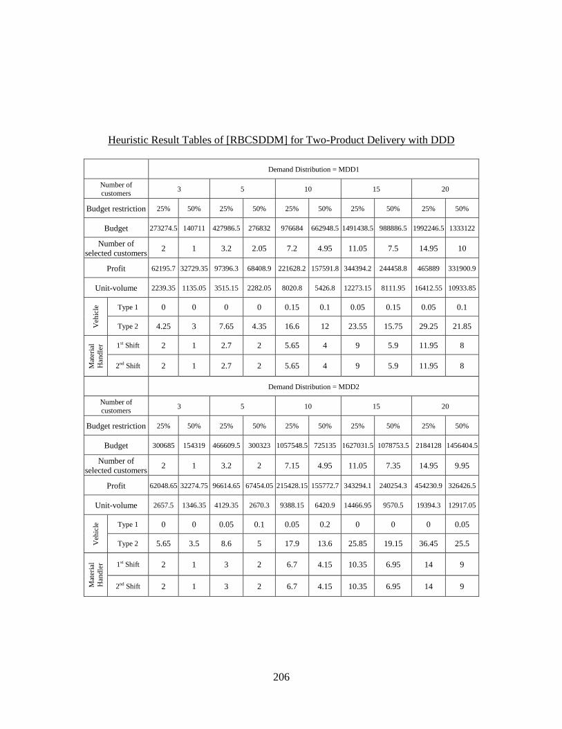
206

Heuristic Result Tables of [RBCSDDM] for Two-Product Delivery with DDD

Demand Distribution = MDD1

Number of

customers 3 5 10 15 20

Budget restriction 25% 50% 25% 50% 25% 50% 25% 50% 25% 50%

Budget 273274.5 140711 427986.5 276832 976684 662948.5 1491438.5 988886.5 1992246.5 1333122

Number of

selected customers 2 1 3.2 2.05 7.2 4.95 11.05 7.5 14.95 10

Profit 62195.7 32729.35 97396.3 68408.9 221628.2 157591.8 344394.2 244458.8 465889 331900.9

Unit-volume 2239.35 1135.05 3515.15 2282.05 8020.8 5426.8 12273.15 8111.95 16412.55 10933.85

Veh

icle

Type 1 0 0 0 0 0.15 0.1 0.05 0.15 0.05 0.1

Type 2 4.25 3 7.65 4.35 16.6 12 23.55 15.75 29.25 21.85

Mat

eria

l

Han

dle

r 1st Shift 2 1 2.7 2 5.65 4 9 5.9 11.95 8

2nd Shift 2 1 2.7 2 5.65 4 9 5.9 11.95 8

Demand Distribution = MDD2

Number of

customers 3 5 10 15 20

Budget restriction 25% 50% 25% 50% 25% 50% 25% 50% 25% 50%

Budget 300685 154319 466609.5 300323 1057548.5 725135 1627031.5 1078753.5 2184128 1456404.5

Number of

selected customers 2 1 3.2 2 7.15 4.95 11.05 7.35 14.95 9.95

Profit 62048.65 32274.75 96614.65 67454.05 215428.15 155772.7 343294.1 240254.3 454230.9 326426.5

Unit-volume 2657.5 1346.35 4129.35 2670.3 9388.15 6420.9 14466.95 9570.5 19394.3 12917.05

Veh

icle

Type 1 0 0 0.05 0.1 0.05 0.2 0 0 0 0.05

Type 2 5.65 3.5 8.6 5 17.9 13.6 25.85 19.15 36.45 25.5

Mat

eria

l

Han

dle

r 1st Shift 2 1 3 2 6.7 4.15 10.35 6.95 14 9

2nd Shift 2 1 3 2 6.7 4.15 10.35 6.95 14 9

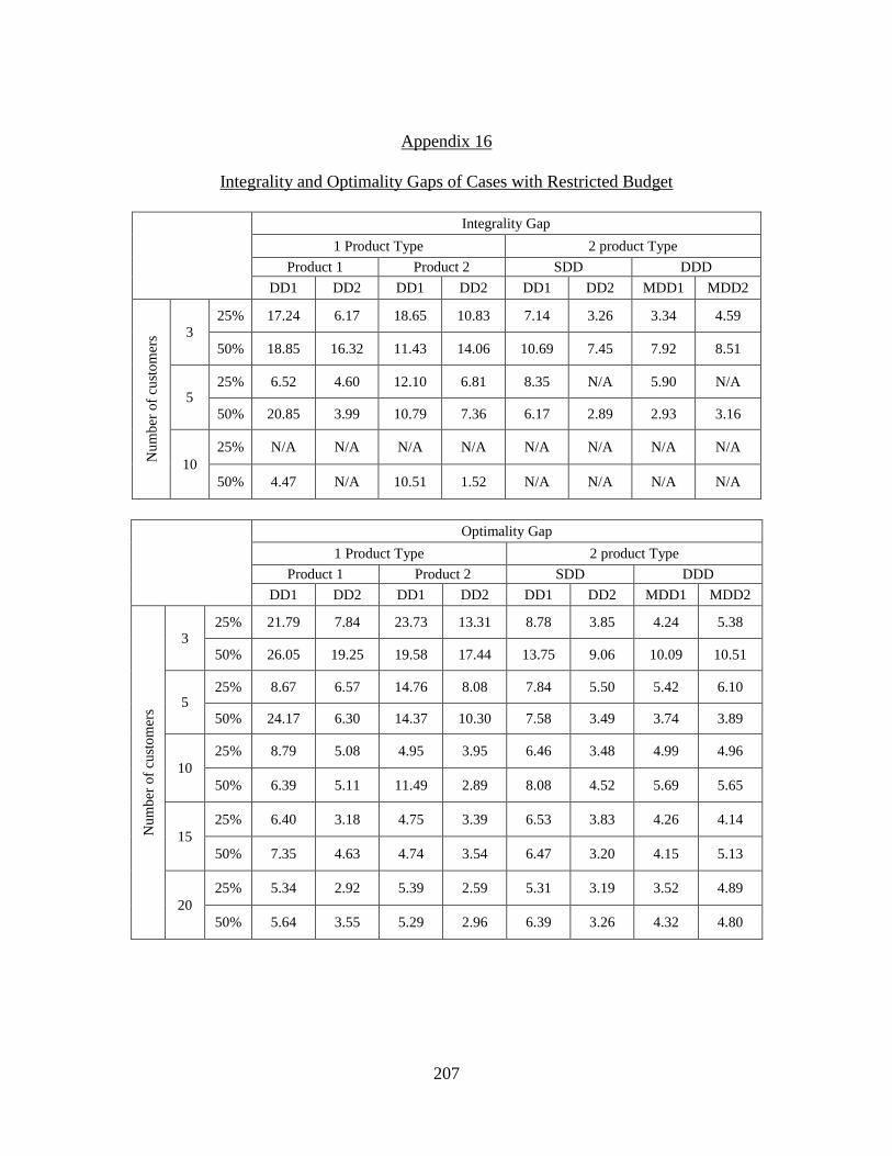
207

Appendix 16

Integrality and Optimality Gaps of Cases with Restricted Budget

Integrality Gap

1 Product Type 2 product Type

Product 1 Product 2 SDD DDD

DD1 DD2 DD1 DD2 DD1 DD2 MDD1 MDD2

Nu

mb

er o

f cu

sto

mer

s 3 25% 17.24 6.17 18.65 10.83 7.14 3.26 3.34 4.59

50% 18.85 16.32 11.43 14.06 10.69 7.45 7.92 8.51

5 25% 6.52 4.60 12.10 6.81 8.35 N/A 5.90 N/A

50% 20.85 3.99 10.79 7.36 6.17 2.89 2.93 3.16

10

25% N/A N/A N/A N/A N/A N/A N/A N/A

50% 4.47 N/A 10.51 1.52 N/A N/A N/A N/A

Optimality Gap

1 Product Type 2 product Type

Product 1 Product 2 SDD DDD

DD1 DD2 DD1 DD2 DD1 DD2 MDD1 MDD2

Nu

mb

er o

f cu

sto

mer

s

3 25% 21.79 7.84 23.73 13.31 8.78 3.85 4.24 5.38

50% 26.05 19.25 19.58 17.44 13.75 9.06 10.09 10.51

5 25% 8.67 6.57 14.76 8.08 7.84 5.50 5.42 6.10

50% 24.17 6.30 14.37 10.30 7.58 3.49 3.74 3.89

10

25% 8.79 5.08 4.95 3.95 6.46 3.48 4.99 4.96

50% 6.39 5.11 11.49 2.89 8.08 4.52 5.69 5.65

15

25% 6.40 3.18 4.75 3.39 6.53 3.83 4.26 4.14

50% 7.35 4.63 4.74 3.54 6.47 3.20 4.15 5.13

20

25% 5.34 2.92 5.39 2.59 5.31 3.19 3.52 4.89

50% 5.64 3.55 5.29 2.96 6.39 3.26 4.32 4.80

208

REFERENCES

Aghezzaf, E., B.Raa, and H.V. Landeghem. 2006. ―Modeling inventory routing problems

in supply chains of high consumption products,‖ European Journal of Operational

Research 169 (2006): 1048-1063.

Anily, S. and A.Federgruen. 1990. ―One warehouse multiple retailer systems with vehicle

routing costs,‖ Management Science 36 (1): 92-114.

Arsham, H. 2008. ―Deterministic modeling: linear optimization with applications,‖

< http://home.ubalt.edu/ntsbarsh/opre640a/partVIII.htm#rplp> accessed [July 16,

2008]

Berman, O. and R.C.Larson. 2001. ―Deliveries in an inventory/routing problem using

stochastic dynamic programming,‖ Transportation Science 35 (2): 192-213.

Bonabeau, E. 2002. ―Agent-based Modeling: Methods and Techniques for Simulating

Human Systems,‖ Proceedings of the National Academy of Sciences of the United

States of America 99: 7280–7287.

Brandão, J. 2004. ―A tabu search algorithm for the open vehicle routing problem,‖

European Journal of Operational Research. 157 (2004): 552-564.

Bräysy, O. and M. Gendreau. 2005a. ―Vehicle routing problem with time windows, part

I: route construction and local search algorithms,‖ Transportation Science 39 (1):

104-118.

Bräysy, O. and M. Gendreau. 2005b. ―Vehicle routing problem with time windows, part

II: metaheuristics,‖ Transportation Science 39 (1): 119-139.

Bronzini, M. and R.Kicinger. 2006. ―Conceptual model of a self-organizing traffic

management hazard response system,‖ Transportation Research Board 2006

Annual Meeting CD-ROM.

Campbell, A.M. and M.W.P. Savelsbergh. 2004. ―A decomposition approach for the

inventory-routing problem,‖ Transportation Science 38 (4): 488-502.

Campos, V. and E.Mota. 2000. ―Heuristic procedures for the capacitated vehicle routing

problem,‖ Computational Optimization and Applications 16: 265-277.

209

Carson, Y. and A.Maria. 1997. ―Simulation optimization: methods and applications,‖ In

Proceedings of the 1997 Winter Simulation Conference, eds. S. Andradóttir, K.J.

Healy, D.H.Withers, and B.L.Nelson: 118-126.

Chan, S. and G. Harris. 2005. ―Hurricane and Floods Overwhelmed Hospitals,‖ The New

York Times, September 14, 2005.

Chang, E.C.P. 2003. ―Traffic simulation for effective emergency evacuation,‖ Oak Ridge

National Laboratory, Oak Ridge, TN.

Chen, X. 2003. ―Agent-based Simulation of Evacuation Strategies under Different Road

Network structures,‖

<http://www.ucgis.org/summer03/studentpapers/xuweichen.pdf> [accessed July 16,

2008].

Chiu, Y.C., H.Zheng, J.Villalobos, and B.Gautam. 2007. ―Modeling no-notice mass

evacuation using a dynamic traffic flow optimization model,‖ IIE Transactions 39:

83-94.

Church, R.L. and R. Sexton. 2002. ―Modeling Small Area Evacuation: Can Existing

Transportation Infrastructure Impede Public Safety? California Department of

Transportation. Testbed Center for Interoperability,‖.

<http://www.ncgia.ucsb.edu/vital/research/pubs/200204-Evacuation.pdf> [accessed

July 16, 2008].

Cohen, M.A. and H.L.Lee. 1988. ―Strategic analysis of integrated production-distribution

systems: models and methods,‖ Operations Research 36 (2): 216-228.

Cordone, R. and R.W.Calvo. 2001. ―A heuristic for the vehicle routing problem with time

windows,‖ Journal of Heuristics 7 :107-129.

Cova, T.J. and J.P. Johnson. 2003. ―A network flow model for lane-based evacuation

routing,‖ Transportation Research Part A 37(7): 579–604.

Crevier, B., J.Cordeau, G.Laporte. 2007. ―The multi-depot vehicle routing problem with

inter-depot routes,‖ European Journal of Operational Research 176(2007): 756-773.

de Silva, F.N., R.W. Eglese, and M. Pidd. 2003. ―Evacuation planning and spatial

decision making: designing effective spatial decision support systems through

integration of technologies,‖ In Decision making support systems: achievements,

trends and challenges for. Idea Group Publishing, p 358–373.

210

Dondo, R. and J.Cerdá. 2007. ―A cluster-based optimization approach for the multi-depot

heterogeneous fleet vehicle routing problem with time windows,‖ European Journal

of Operational Research 176: 1478-1507.

FEMA/Corps Hurricane Study Program, 1986-2006. ―Summary Report Completed in

Summer 2000-South Carolina Hurricane Evacuation Study,‖

<http://chps.sam.usace.army.mil/USHESdata/SC/SCmainreportpage.htm >,

[accessed July 16, 2008].

Fu, Z., R. Eglese, and Li, L.Y.O. 2005. ―A new tabu search heuristic for the open vehicle

routing problem,‖ Journal of the Operational Research Society 56 (2005): 267-274.

Gladwin, C.H., H. Gladwin, and W.G. Peacock. 2001. ―Modeling hurricane evacuation

decisions with ethnographic methods,‖ International Journal of Mass Emergencies

and Disasters 19(2): 117–143.

Hashimoto, H., T.Ibaraki, S.Imahori, and M.Yagiura. 2006. ―The vehicle routing problem

with flexible time window and traveling times,‖ Discrete Applied Mathematics 154

(2006): 2271-2290.

Henrion, R. 2004. ―Introduction to Chance-Constrained Programming‖.

< http://stoprog.org/index.html?SPIntro/intro2ccp.html>, [accessed July 16, 2008].

Ho, W., G.T.S.Ho, P.Ji, and H.C.W.Lau. 2008. ―A hybrid genetic algorithm for the multi-

depot vehicle routing problem,‖ Engineering Applications of Artificial Intelligence

21(2008): 548-557.

Hobeika, A.G. and B. Jamei. 1985. ―MASSVAC: A model for calculating evacuation

times under natural disaster,‖ Emergency Planning, Simulation Series 15: 23–28.

Hobeika, A.G. and C. Kim. 1998. ―Comparison of traffic assignments in evacuation

modeling,‖ IEEE Transactions on Engineering Management 45(2): 192–198.

Holmes, Derek. ―What is Stochastic Programming?‖.

<http://users.iems.northwestern.edu/~jrbirge/html/dholmes/StoProIntro.html>

[accessed July 16, 2008]

Hospital Incident Command System Guidebook. 2006.

< http://www.emsa.ca.gov/HICS/files/Guidebook_Glossary.pdf >, [accessed July

16, 2008]

Law, A.M. and W.D.Kelton. 2000. Simulation Modeling and Analysis. 3rd

Ed. New York:

McGraw-Hill: 253-259.

211

Le Bouthillier, A. and T.G.Crainic. 2005. ―A cooperative parallel meta-heuristic for the

vehicle routing problem with time windows,‖ Computers & Operations Research 32

(2005): 1685-1708.

Li, F., B.Golden, E.Wasil. 2007. ―The open vehicle routing problem: Algorithms, large-

scale test problems, and computational results,‖ Computers & Operations Research

34 (2007) : 2918-2930.

Liu, H.X., J.X.Ban, W.Ma, P.B.Mirchandani. 2006. ―Model reference adaptive control

framework for real time traffic management under emergency evacuation,‖

Transportation Research Board 2006 Annual Meeting CD-ROM.

Liu, S.C. and S.B.Lee. 2003. ―A two-phase heuristic method for the multi-depot location

routing problem taking inventory control decisions into consideration,‖

International Journal of Advanced Manufacturing Technology (2003) 22: 941-950.

Liu, S.C. and C.C.Lin. 2005. ―A heuristic method for the combined location and

inventory problem,‖ International Journal of Advanced Manufacturing Technology

(2005) 26: 372-381.

McGlown, K.J. 1999. ―Determinants of the Evacuation of Health Care Facilities. Ph.D.

Dissertation,‖ University of Alabama at Birminham.

McGlown, K.J. 2001. ―Evacuation of Health Care Facilities: A New Twist to a Classic

Model,‖ Natural HazardsReview 2(2): 90–99.

Ozdamar, L., E.Ekinci, and B.Kucukyazici. 2004. ―Emergency Logistics Planning in

Natural Disasters,‖ Annals of Operations Research 129: 217-245.

Perry, R.W. and M.K. Lindell. 1991. ―The Effects of Ethnicity on Evacuation Decision-

Making,‖ International Journal of Mass Emergencies and Disasters 9(1): 47–68.

Pidd, M., F.N. de Silva, and R.W. Eglese. 1996. ―A simulation model for emergency

evacuation,‖ European Journal of Operational Research 90(1996): 413–419.

Pisinger, D. and S.Ropke. 2007. ―A general heuristic for vehicle routing problems,‖

Computers & Operations Research 34 (2007): 2403-2435.

Pollak, E., M. Falash, L. Ingraham, and V. Gottesman. 2004. ―Operational analysis

framework for emergency operations center preparedness training,‖ In Proceedings

of the 2004 Winter Simulation Conference, eds. R. G. Ingalls, M.D. Rosetti,

J.S.Smith, and B.A.Peters: 839–848.

212

Raa, B. and E.Aghezzaf. 2008. ―Designing distribution patterns for long-term inventory

routing with constant demand rates,‖ International Journal of Production Economics

112 (2008):2 55-263.

Radwan, E., M. Mollaghasemi, S. Mitchell, and G. Yildirim. 2005. ―Framework for

modeling emergency evacuation,‖ Final project report submitted to Florida

Department of Transportation, April 2005. < http://www.dot.state.fl.us/Research-

Center/Completed_Proj/Summary_TE/FDOT_BD548_05_rpt.pdf> [accessed July

16, 2008].

Repoussis, P.P., C.D. Tarantilis, and G.Ioannou. 2007. ―The open vehicle routing

problem with time windows,‖ Journal of the Operational Research Society

58(2007): 355-367.

Rockwell Automation. 2006. OptQuest for Arena User’s Guide.

Rohde, D., D.G. Mcneil Jr., R. Abelson and S. Dewan, 2005 ―154 Patients Died, Many in

Intense Heat, as Rescues Lagged.‖ Global Action on Aging.

<http://www.globalaging.org/armedconflict/countryreports/americas/154died.htm>

[accessed July 16, 2008].

Russell, R.A. and W.Chiang. 2006. ―Scatter Search for the vehicle routing problem with

time windows,‖ European Journal of Operational Research 169 (2006): 606-622.

Qu, W.W., J.H.Bookbinder, and P.Iyogun. 1999. ―An integrated inventory-transportation

system with modified periodic policy for multiple products,‖ European Journal of

Operational Research 115 (1999): 254-269.

Quarantelli, E.L. 1980. ―Evacuation Behavior and Problems: Findings and Implications

from the Research Literature,‖ Disaster Research Center. Ohio State University,

Columbus, Ohio.

Santos, G. and B.E. Aguirre. 2004. ―A Critical Review of Emergency Evacuation

Simulation Models,‖ NIST Workshop on Building Occupant Movement during Fire

Emergencies, 27–52. <http://www.fire.nist.gov/bfrlpubs/fire05/PDF/f05012.pdf>

[accessed December 10, 2006].

Sariklis, D. and S.Powell. 2000. ―A heuristic method for the open vehicle routing

problem,‖ Journal of the Operational Research Society 51(2000): 564-573.

Savalsbergh, M. and J.Song. 2007. ―Inventory routing with continuous moves,‖

Computers & Operations Research 34 (2007): 1744-1763.

213

Savalsbergh, M. and J.Song 2008. ―An optimization algorithm for the inventory routing

problem with continuous moves,‖ Computers & Operations Research 35 (2008):

2266-2282.

Sbayti, H. and H.S.Mahmassani. 2006. ―Optimal scheduling of evacuation operations,‖

Transportation Research Board 2006 Annual Meeting CD-ROM.

Sheffi, Y., H. Mahmassani, and W.B. Powell. 1982. ―A Transportation Network

Evacuation Model,‖ Transportation Research Part A 16(3): 209–218.

Shen, Z.M. and L.Qi. 2007. ―Incorporating inventory and routing costs in strategic

location models,‖ European Journal of Operational Research 179 (2007): 372-389.

Sisiopiku, V.P. 2007. ―Application of traffic simulation modeling for improved

emergency preparedness planning,‖ Journal of Urban Planning and Development

133 (1): 51-60.

Sorensen, J.H. and D. Mileti. 1987. ―Decision-making uncertainties in emergency

warning system organization,‖ International Journal of Mass Emergencies and

Disasters 5 (1):33–62.

Sorensen, J.H. 1991. ―When Shall We Leave? Factors Affecting the Timing of

Evacuation Departures,‖ International Journal of Mass Emergencies and Disasters

9(2): 153–165.

Song, J. and M. Savelsbergh. 2007. ―Performance measurement for inventory routing,‖

Transportation Science 41 (1): 44-54.

South Carolina Department of Health and Environmental Control (SCDHEC). 2004.

―State of South Carolina Department of Health and Environmental Control

Emergency Order ,‖ < http://www.scdhec.net/health/licen/hleo.pdf >[accessed July

16, 2008].

Swisher, J.R. and P.D.Hyden. 2000. ―A survey of simulation optimization techniques and

procedures,‖ In Proceedings of the 2000 Winter Simulation Conference, eds. J.A.

Joines, R. R. Barton, K. Kang, and P. A. Fishwick: 119-128.

Taaffe, K., R. Kohl, and D.L. Kimbler. 2005. ―Hospital Evacuation: Issues and

Complexities,‖ Proceedings of the 2005 Winter Simulation Conference, ed. M.E.

Kuhl, N.M. Steiger, F.B. Armstrong, and J.A. Joines, 943–950.

Tan, K.C., L.H.Lee, Q.L.Zhu, and K.Ou. 2001. ―Heuristic methods for vehicle routing

problem with time windows,‖ Artificial Intelligence in Engineering 15 (2001): 281-

295.

214

Tanaka, K., T.Nagatani, and H. Hanaura. 2006. ―Traffic congestion and dispersion in

hurricane evacuation,‖ Physica A (2006).

Tarantilis, C.D., G.Ioannou, C.T.Kiranoudis, and G.P.Prastacos. 2005. ―Solving the open

vehicle routing problem via a single parameter metaheuristic algorithm,‖ Journal of

the Operational Research Society 56(2005): 588-596.

Thangiah, S.R. and S.Salhi. 2001. ―Genetic clustering: an adaptive heuristic for the multi-

depot vehicle routing problem,‖ Applied Artificial Intelligence 15(4): 361-383.

Tovia, F. 2007. ―An emergency logistics response system for natural disasters,‖

International Journal of Logistics: Research and Applications 10 (3): 173-186.

Tufekci, S. 1995. ―An integrated emergency management decision support system for

hurricane emergencies,‖ Safety Science 20 (1995): 39-48.

Urbina, E. and B.Wolshon. 2003. ―National review of hurricane evacuation plans and

policies: a comparison and contrast of state practices,‖ Transportation Research Part

A 37 (2003): 257-275.

U.S. Government Accountability Office (GAO). 2006. ―GAO-06-443R: Preliminary

Observations on the Evacuation of Hospitals and Nursing Homes due to Hurricanes.

February 16, 2006,‖ <http://www.gao.gov/new.items/d06443r.pdf> [accessed July

16, 2008].

Vogt, B.M. 1990. ―Evacuation of Institutionalized and Specialized Populations,‖ Oak

Ridge National Laboratory, Oak Ridge, TN.

Vogt, B.M. 1991. ―Issues in Nursing Home Evacuations,‖ International Journal of Mass

Emergencies and Disasters 9(2): 247–265.

Wolshon, B., E.Urbina, C.Wilmot, and M.Levitan. 2005a. ―Review of policies and

practices for hurricane evacuation I: Transportation planning, preparedness, and

response,‖ Natural Hazards Review 6 (3): 129-142.

Wolshon, B., E.Urbina, M.Levitan, and C.Wilmot. 2005b. ―Review of policies and

practices of hurricane evacuation II: Traffic operations, management, and control,‖

Natural Hazards Review 6 (3): 143-161.

Zhao, Q., S.Wang, and K.K.Lai. 2007. ―A partition approach to the inventory/routing

problem,‖ European Journal of Operational Research 177 (2007): 786 - 802.