Optimal Scheduling and Allocation for IC Design … · Optimal Scheduling and Allocation for IC...

60

Optimal Scheduling and Allocation for IC Design Managementand Cost Reduction

PRABHAV AGRAWAL, UC San DiegoMIKE BROXTERMAN, Qualcomm, Inc.BISWADEEP CHATTERJEE, Qualcomm India Private LimitedPATRICK CUEVAS and KATHY H. HAYASHI, Qualcomm, Inc.ANDREW B. KAHNG, PRANAY K. MYANA, and SIDDHARTHA NATH, UC San Diego

A large semiconductor product company spends hundreds of millions of dollars each year on design infras-tructure to meet tapeout schedules for multiple concurrent projects. Resources (servers, electronic designautomation tool licenses, engineers, and so on) are limited and must be shared – and the cost per day ofschedule slip can be enormous. Co-constraints between resource types (e.g., one license per every two cores(threads)) and dedicated versus shareable resource pools make scheduling and allocation hard. In this ar-ticle, we formulate two mixed integer-linear programs for optimal multi-project, multi-resource allocationwith task precedence and resource co-constraints. Application to a real-world three-project scheduling prob-lem extracted from a leading-edge design center of anonymized Company X shows substantial compute andlicense costs savings. Compared to the product company, our solution shows that the makespan of scheduleof all projects can be reduced by seven days, which not only saves ∼2.7% of annual labor and infrastructurecosts but also enhances market competitiveness. We also demonstrate the capability of scheduling over twodozen chip development projects at the design center level, subject to resource and datacenter capacity lim-its as well as per-project penalty functions for schedule slips. The design center ended up purchasing 600additional servers, whereas our solution demonstrates that the schedule can be met without having to pur-chase any additional servers. Application to a four-project scheduling problem extracted from a leading-edgedesign center in a non-US location shows availability of up to ∼37% headcount reduction during a half-yearschedule for just one type of chip design activity.

Categories and Subject Descriptors: B.7.2 [Design Aids]: Design Schedule and Cost Optimization

General Terms: Design, Optimization

Additional Key Words and Phrases: Design cost optimization, resource scheduling, project scheduling

ACM Reference Format:Prabhav Agrawal, Mike Broxterman, Biswadeep Chatterjee, Patrick Cuevas, Kathy H. Hayashi, AndrewB. Kahng, Pranay K. Myana, and Siddhartha Nath. 2017. Optimal scheduling and allocation for IC designmanagement and cost reduction. ACM Trans. Des. Autom. Electron. Syst. 22, 4, Article 60 (June 2017), 30pages.DOI: http://dx.doi.org/10.1145/3035483

Authors’ addresses: P. Agrawal, A. B. Kahng, P. K. Myana, and S. Nath, Department of Computer Scienceand Engineering, University of California at San Diego, La Jolla, CA 92093; M. Broxterman, P. Cuevas,and K. H. Hayashi, Qualcomm Inc., 5775 Morehouse Drive, San Diego, CA 92121; B. Chatterjee, QualcommTechnology India Pvt. Ltd., Plot 153-154, EPIP, Phase II, Whitefield, Bangalore KA 560066.Permission to make digital or hard copies of part or all of this work for personal or classroom use is grantedwithout fee provided that copies are not made or distributed for profit or commercial advantage and thatcopies show this notice on the first page or initial screen of a display along with the full citation. Copyrights forcomponents of this work owned by others than ACM must be honored. Abstracting with credit is permitted.To copy otherwise, to republish, to post on servers, to redistribute to lists, or to use any component of thiswork in other works requires prior specific permission and/or a fee. Permissions may be requested fromPublications Dept., ACM, Inc., 2 Penn Plaza, Suite 701, New York, NY 10121-0701 USA, fax +1 (212)869-0481, or [email protected]© 2017 ACM 1084-4309/2017/06-ART60 $15.00DOI: http://dx.doi.org/10.1145/3035483

ACM Transactions on Design Automation of Electronic Systems, Vol. 22, No. 4, Article 60, Pub. date: June 2017.

http://dx.doi.org/10.1145/3035483

http://dx.doi.org/10.1145/3035483

60:2 P. Agrawal et al.

1. INTRODUCTION

Since 2001, the International Technology Roadmap for Semiconductors [ITRS] chap-ter on Design Technology has presented a Design Cost model calibrated to mobilesystem-on-chip (SOC) products (e.g., Qualcomm Snapdragon [Snapdragon] andSamsung Exynos [Exynos]) that are the main processing cores of tablets and smart-phones and their associated development costs [Chan et al. 2014; Kahng and Smith2002; Smith 2014]. For well over a decade, the Design Cost model has documented de-sign costs of tens of millions of dollars for a single SOC product. Major contributors todesign cost include engineering headcount, compute infrastructure (servers, filers, dat-acenters), and electronic design automation (EDA) tool licenses. The large investmentrequirement for new product development stifles semiconductor startup activity andinnovation, and has arguably contributed to consolidation and a slowdown of growthfor the industry.

Today, a large semiconductor product company will spend hundreds of millions ofdollars annually on design infrastructure (e.g., datacenters, EDA tools, design teams)to meet tapeout schedules for multiple concurrent projects. Resources (e.g., servers,licenses, engineers) are limited and must be shared across projects. Not only are sched-ule slips extremely costly but, as highlighted in recent years (e.g., the “How Green isMy Silicon Valley” plenary panel at the 2009 Design Automation Conference (DAC)[DAC09]), there is now tremendous concern to reduce the energy footprint of semicon-ductor integrated circuit (IC) design. In contrast to traditional scheduling optimizationsseen in the operations research and industrial engineering literature, IC design flowsoften exhibit co-constraints between resource types (e.g., one license needed per everytwo cores used in a multi-threaded tool run1). Common design center practices, suchas the setting up of dedicated vs. shareable resource pools as permitted by LSF-typegridware [LSF], also make scheduling and allocation hard. Further, design managers,while increasingly able to track and diagnose design activity [Fenstermaker et al. 2000;RTDA], have no decision support tools to help determine the resource investments (e.g.,is it better to add 500 more servers or 50 more timing analysis tool licenses?) that en-able schedule requirements to be met with minimum cost. Thus, a company may leavemillions of dollars and gigawatt-hours per year – as well as weeks of schedule time – onthe table. In a competitive and cost-driven industry, there is an urgent need to recoversuch wasted resources.

In the field of operations research, Kolisch and Hartmann [1999], Kolisch et al.[1992], and Kolisch and Sprecher [1996] give an integer-linear programming (ILP) for-mulation to solve the resource-constrained project scheduling problem (RCPSP). Theformulation optimally allocates renewable, non-renewable, and doubly-constrained re-sources across multiple activities (with precedence constraints) in a project. The objec-tive of the formulation is to minimize the makespan of a project with multiple activities.We extend this formulation in the context of IC design cost optimization in various ways.Specifically, we describe two mixed integer-linear programming (MILP) formulationsthat efficiently and optimally perform multi-project, multi-resource allocation withcomplex task precedence and resource co-constraints. The first is the Schedule CostMinimization (SCM) formulation, and the second is the Resource Cost Minimization(RCM) formulation. We solve these two general resource-constrained project schedulingproblems that arise in a multi-tenanted, heterogeneous, high-throughput computing(HTC) environment. A problem instance consists of projects that can be scheduled

1Maintaining design schedules with constant engineering headcount, even as SOC complexities continue toscale, increasingly relies on multithreading (e.g., detailed routing, static timing analysis, physical verifica-tion) and/or massively distributed tool runs (e.g., to perform functional verification).


Optimal Scheduling and Allocation for IC Design Management and Cost Reduction 60:3

in parallel, each involving multiple activities, in which each activity must consumeprescribed amounts of resources to reach completion. The goal is to schedule the projectseither with minimum total loss according to given penalty functions or with minimumnumber of resources consumed per time unit.2 In Section 4.1, we describe an instancewith three projects, 11 activities with various precedence constraints per project, andfive types of resources that must be completed within 90 days. Our MILP formulationcaptures such types of problems in a straightforward manner, as we demonstrate inSection 4.1.

The challenge in practice for a large semiconductor design organization is to providejust-in-time resources for each project, such that (i) project execution is not delayed byresource starvation and (ii) utilization of each resource type satisfies resource limitsor usage policies. Current industry dynamics lead to strict boundary conditions (e.g.,time-to-market, tapeout deadline), and constrained capital spending pushes businessunits to seek increased productivity through maximum utilization of existing resources.Today, resource planning and allocation, especially involving allocation of multiple dis-parate resource types, has largely been dictated by heuristics and historical experience.Decision support is urgently needed for “course corrections” and understanding of theimpact of resource allocation decisions. With this as background, our main contribu-tions are as follows.

(1) We model two resource-constrained optimal project scheduling formulations, SCMand RCM, as MILPs. Our formulations handle multiple projects, multiple activitieswith precedence constraints, and multiple types of resources.3

(2) We handle co-constraints between resource types and allocation of resources frommultiple (fully-shared, conditionally-shared, segregated) resource pools. Each poolmay have a different penalty function, capturing real-world scenarios in a largeSOC design company. To our knowledge, we are the first to consider co-constraintsbetween resource types.

(3) We optionally enforce stability constraints that upper-bound the change in aproject’s allocated resources between successive timesteps.

(4) Application of SCM to a three-project scheduling problem extracted from a leading-edge design center of Company X4 shows substantial compute and license costsavings compared to the actual allocation/scheduling solution used by the productcompany. Our solution reduces the schedule makespan of all projects by 1.4 work-weeks,5 i.e., ∼2.7% of annual design infrastructure cost. (Per “Moore’s Law,” thesemiconductor industry advances at ∼1% in a calendar week [Moore’s Law]. There-fore, during this time, the semiconductor industry advances by more than 1%.) Wealso demonstrate the scheduling of two dozen chip development projects at the de-sign center level, subject to resource and datacenter capacity limits as well as per-project penalty functions for schedule slips. The design center was unable to solvethis problem and ended up purchasing 600 additional servers to avoid schedule

2A typical real-world HTC environment has multiple concurrent projects – each working on a specificschedule that is largely non-negotiable and each having different workload characteristics in terms of in-frastructure requirements.3Note that we do not solve arbitrary-sized MILP formulations in this work. The context of our formulationand ranges of our inputs pertain to IC design projects; very few, if any, semiconductor companies in the realworld would face problem instances with complexities larger than what we study in the article. Further, webelieve that on the time scales of SOC implementation, even a couple of days of runtime is tolerable if thereturn is weeks of schedule gain or millions of dollars of design cost reductions.4Owing to confidentiality reasons, we cannot reveal the name of the company; we refer to it as Company X.5In the semiconductor industry, we typically refer to one “work-week” as five working days in a week.



Table I. Representative Previous Works

Reference Formulation Objective Modes PreemptiveResource

Co-constraintsConditionally-Shared

ResourcesAyala and Artigues [2010] ILP throughput ✗ ✗ ✗ ✗

Baptiste and Demassey[2004]

LP makespan ✗ ✗ ✗ ✗

Bienstock andZuckerberg [2009]

LP cost � � ✗ ✗

Bonfietti et al. [2014] CP throughput ✗ � ✗ ✗

Christofides et al. [1987] ILP, LP cost ✗ � ✗ ✗

Keller and Bayraksan[2009]

Stochastic ILP cost ✗ ✗ ✗ ✗

Kolisch et al. [1992],Kolisch and Sprecher

[1996]

ILP makespan � ✗ ✗ ✗

Kramer and Hwang[1991]

MILP, LP cost � � ✗ ✗

Li et al. [2009] MILP makespan ✗ � ✗ ✗

Mohanty and Nayak[2011]

PSO cost ✗ � ✗ ✗

Qiong et al. [2010] ACO makespan ✗ ✗ ✗ ✗

Salewski et al. [1997] ILP cost � ✗ ✗ ✗

Our work MILP cost/makespan ✗ � � �

slips. Our solution shows that the schedule requirements could have been metwithout purchasing any additional servers.

(5) Application of RCM to a four-project scheduling problem extracted from a leading-edge design center of Company X shows substantial human resource costs left onthe table by the actual allocation/scheduling solution used by the company. For aparticular activity related to chip design, our solution reduces headcount by 37%,which translates to ∼$3.7 million in savings at that particular (non-US) designcenter. Our solver can also provide decision support via “what-if” analyses of costand schedule trade-offs.

(6) Of separate interest is the description of our test-case generator that we use toperform scalability and sensitivity studies. We propose to make our generator andsolvers open-source, as prototyped at MILP-Solver.

The remainder of this article is organized as follows. Section 2 reviews relevant priorwork. Section 3 describes our MILP formulations. In Section 4, we describe experi-mental validation of benefits from our MILP formulations, using three instances froma worldwide top-5 semiconductor company. We present our conclusions and outlinefuture work in Section 5.

2. RELATED WORK

Resource-constrained project scheduling has been solved in many different settingswith varying constraints and/or objective functions. Table I places our present workin the context of representative previous works on resource scheduling with multipleactivities. A common objective is to minimize the makespan [Baptiste and Demassey2004]. Objective functions studied typically minimize project cost given time-dependentand/or resource-dependent penalties [Kramer and Hwang 1991; Talbot 1982].

Several previous works solve the scheduling problem for a single project with mul-tiple activities [Bienstock and Zuckerberg 2009; Christofides et al. 1987; Keller andBayraksan 2009; Kolisch and Sprecher 1996; Mohring et al. 2001; Salewski et al. 1997].The activities can be either preemptive or nonpreemptive [Baptiste and Demassey2004; Kolisch and Sprecher 1996; Salewski et al. 1997; Talbot 1982]. Kolisch andSprecher [1996] and Kolisch et al. [1992] formulate the RCPSP and propose methodsto generate RCPSP instances. They present the PSPLIB and MPSPLIB benchmark



suites, along with optimal as well as heuristic solutions.6 Further variations involvethe scheduling of activities that can execute in multiple modes [Bienstock and Zucker-berg 2009; Kolisch and Sprecher 1996; Kramer and Hwang 1991; Salewski et al. 1997;Talbot 1982]. These works consider that the resource usage and the time taken by anactivity can vary across available modes; they provide optimal scheduling solutionsacross combinations of modes of activities. Mohring et al. [2001] and Christofideset al. [1987] provide branch-and-bound algorithms to solve the resource-constrainedmulti-activity single project scheduling problem. Mohring et al. [2001] further tryto identify special cases that are solvable in polynomial time. Generally, solutionframeworks involve linear or integer linear programming, although stochastic [Kellerand Bayraksan 2009] and nonlinear [Bonfietti et al. 2014] formulations have alsobeen studied. Cyclic scheduling has been addressed in Ayala and Artigues [2010] andBonfietti et al. [2014], in which sets of activities are executed indefinitely over time ina periodic fashion. The work of Keller and Bayraksan [2009] is noteworthy in that itsformulation permits temporary resource expansion, albeit for a penalty that featuresin the objective function. This has some similarity to our formulation presented later,which has different penalties for resources used from different resource pools. (Theformulation provided in Keller and Bayraksan [2009] does not include precedenceconstraints within activities or a number of other aspects of our formulation.)

To optimize human resources at an enterprise scale, Li et al. [2009] minimize themakespan of a single project with multiple activities, subject to upper bounds of hu-man resources. Mohanty and Nayak [2011] propose a particle swarm optimization(PSO) algorithm to optimize the trade-off between cost and profit when a given num-ber of employees are assigned to an activity. Their formulation considers employeeswith different skill competencies for different activities. Qiong et al. [2010] propose anant colony optimization (ACO) algorithm to minimize the makespan of a project withmultiple activities and precedence constraints between the activities. The activitiesare assumed to be non-preemptive, and the algorithm is applicable to general parallelmachine-scheduling problems.

Several commercial tools and services exist today [Dassult Systems; IC Manage;inMotion; Nefelus; Salesforce] that serve design project management needs. Some ofthese tools are specific to IC design [Dassult Systems; IC Manage; Nefelus], whereasthe other tools can serve project management needs for any industry. Our work is notcomparable to these tools because our work is combinatorial optimization-based andsolves formulations that, to our knowledge, are not addressed by any commercial prod-uct. We have experimented with multiple tools for forecasting and performing what-ifanalyses. However, none of these commercial tools are flexible to enable analyses indifferent scenarios that large design companies work on, which has led to the develop-ment of custom tools and methods for project planning. Today, large design companiesuse a mix of in-house customer methods, statistical packages, business reporting toolsand large-scale production databases for project planning.

Comparisons to works on datacenter job allocations. Our work uses an objectivefunction similar to that seen in works from the datacenter literature that propose al-gorithms to handle job scheduling within a datacenter, e.g., to minimize the makespanas well as other penalty functions. With energy consumption a major concern in mod-ern datacenters, recent formulations by Friese et al. [2012] propose multi-objectiveoptimization of makespan and energy consumption. However, formulations for data-centers are focused on providing job scheduling solutions either in real-time or “online”

6We have compared optimal solutions from our formulation with the optimal solutions of benchmarks fromPSPLIB in Section 4.



[Li et al. 2014], often by using live data from various thermal, network, and rack uti-lization sensors. By contrast, our optimization is performed “offline,” that is, we donot monitor status of project executions in real-time during the optimization of ourobjective function.

Other distinctions from previous works. While a number of previous works ad-dress optimizations related to resource-constrained project scheduling, they cannotaddress important use cases that arise for large SOC product companies. Our for-mulations address real-world use cases that incorporate the following: (i) resource co-constraints, (ii) tethering forecast resource allocations, and (iii) simultaneous allocationof three different categories of resources (Fully-shared, Segregated, and Conditionally-shared). Our formulations also handle stability constraints so that allocation of re-sources (in particular, engineers) are shuffled as infrequently as possible acrossprojects. This induces a trade-off between schedule cost and frequency of task switch-ing. Overall, we enable management to identify the minimum cost (in terms of anypenalty functions deemed appropriate for the situation) of project completion withina set period of time, capturing many constraint types that arise in the industry. Oursolver can also help analyze how varying resource allocation affects cost and scheduleof product tapeout. We demonstrate a use case of handling late-breaking bugs in oneproject without major disruptions in allocations of other projects.

3. PROBLEM FORMULATIONS

We now present (i) notations used in our discussion, (ii) resource categories that arisein multi-tapeout project scheduling, and (iii) our MILP formulations. We have spentconsiderable time working with technical management at one of a worldwide top-5semiconductor company’s design centers to arrive at the optimization formulationsdescribed later. Table II gives notations used in our work. “I” represents an input tothe MILP and “O” an optimization variable. We also indicate which notations are usedin each of the SCM and RCM formulations.

3.1. Resource Pool Types

Chip design companies typically have three pools for each resource type. Resourcetypes include compute nodes, memory, storage, and people [Qualcomm personal com-munication].

Fully-shared resources are shared across all projects. We use ri, j,k,t to denote thenumber of fully shared resources of type k used by activity a(i, j) of project Pi at timet. For example, if there are two projects P1 and P2 with one activity each and 20 fully-shared resources of type k are available, then P1 and P2 can share these 20 resourcesamong themselves such that r1,1,k,t + r2,1,k,t ≤ 20.

Segregated/dedicated resources are allocated exclusively to a specific project. Theseresources are not available for use by any other projects at any time. We use qi, j,k,t todenote the number of segregated resources of type k used by activity a(i, j) of projectPi, at time t. For example, if there are two projects P1 and P2 with one activity eachand they are respectively allocated 10 and 20 segregated resources of type k, thenq1,1,k,t ≤ 10, and q2,1,k,t ≤ 20.

Conditionally-shared resources are allocated to each project, but any resource un-used by a project may be used by other projects. We use yi, j,k,t to denote the number ofconditionally-shared resources of type k used by activity a(i, j) of project Pi at time t. Forexample, if there are two projects P1 and P2 with one activity each and they are respec-tively allocated 10 and 20 conditionally-shared resources of type k, then y1,1,k,t ≤ 10 andy2,1,k,t ≤ 20. We use the notation zi, j,k,t to denote the number of resources of type k used



Table II. Notations Used in Our Work

Parameter Description I/O FormulationN Total number of projects I SCM, RCMT Maximum duration over all projects; t = 1, 2, . . . , T I SCM, RCMPi Projects indexed by i = 1, 2, . . . , N – SCM, RCMJ(i) Total number of activities for Pi I SCM, RCMai, j Pi ’s activities, where j = 1, 2, . . . , J(i) – SCM, RCMHa(i, j) Set of predecessor activities of ai, j that must complete before ai, j

can startI SCM, RCM

K Available resource types I SCM, RCMRk,t Upper bound (UB) on # resources of type k at time t I SCMHr(i, j, k) Set of predecessor resources for resource type k for ai, j I SCMg(i, j, h, k, t) Function that sets a UB on # resource type k at any time t, for

each predecessor h ∈ Hr(i, j, k)I SCM

Li, j,k # resources of type k required to complete ai, j I SCM, RCMUk,t UB on # fully-shared resources of type k at time t I SCMUk UB on # fully-shared resources of type k at any time t O RCMVi,k,t UB on # segregated resources of type k for Pi at time t I SCMMi,k,t UB on # conditionally-shared resources of type k for Pi at time t I SCMGi,k,t UB on total # resources of type k used by Pi at time t I SCM, RCMBi,k,t UB on change in resources consumed by Pi from t − 1 to t I SCM, RCMdnom

i, j (enomi ) Nominal duration of ai, j (Pi) I SCM, RCM

Cai, j (t) (C p

i (t)) Penalty function for ai, j (Pi) at time t I SCM, RCMCk Weight for resource type k I RCMC Cost of switching activities/projects I SCM+wi, j,k,t # resources of type k consumed by ai, j at time t, given by forecast

resource allocationI SCM

δ % of variation allowed in wi, j,k,t I SCMsnomi, j ( f nom

i, j ) Nominal start (finish) time of ai, j for tethering constraints I SCM, RCMri, j,k,t # fully-shared resources of type k consumed by ai, j at time t O SCM, RCMqi, j,k,t # segregated resources of type k consumed by ai, j at time t O SCMyi, j,k,t # conditionally-shared resources of type k consumed by ai, j at

time tO SCM

zi, j,k,t # unused conditionally-shared resources of type k consumed byai, j at time t

O SCM

si, j ( fi, j ) Start (finish) time of ai, j O SCM, RCMSi, j,t (Fi, j,t) 0-1 variable, set to 1 if t ≥ si, j (t ≥ fi, j ); 0 otherwise O SCM, RCM

by activity a(i, j) of project Pi at time t from the pool of unused conditionally-sharedresources of other projects. In the preceding example, we have z1,1,k,t ≤ 20 − y2,1,k,t andz2,1,k,t ≤ 10 − y1,1,k,t.

Figure 1 illustrates two scenarios with three projects: A, B, and C. Each project hasone activity and consumes resource type k at time t. Each project may use resourcesfrom any of the three pools with the following constraints: (i) segregated resources qi, j,k,tconsumed by a project cannot exceed the upper bound Vi,k,t, as shown in Figure 1, and(ii) conditionally-shared resources yi, j,k,t consumed by a project cannot exceed Mi,k,t.Figure 1(a) shows a feasible allocation of resources from each pool. Projects A and Bhave a total of eight units of unused resources in their conditionally-shared pools afterallocation of resources from each pool.7 Project C uses five out of these eight units, i.e.,zC, j,k,t = 5. The total number of fully-shared resources consumed by all three projects,

7Projects A, B, and C use 4, 4, and 5 resources from their respective segregated pools, which are within theupper bounds VA,k,t = VB,k,t = VC,k,t = 5.



Fig. 1. Examples showing (a) feasible and (b) infeasible allocations of resources among three projects, A, B,and C.

i.e., 3+2+6 = 11, cannot exceed Uk,t = 20. Figure 1(b) shows an allocation of resourcesthat is infeasible because yC, j,k,t = 6 > MC,k,t = 5. Furthermore, project C uses moreresources from the unused conditionally-shared resource pool label, i.e., zC, j,k,t > 8.

3.2. MILP Description of the Schedule Cost Minimization Formulation

Given the inputs listed in Table II for the SCM formulation, we seek to minimize thetotal cost (i.e., sum of schedule penalties) of all projects:

minimizeN∑

i=1

T∑t=1

C pi (t) +

N∑i=1

J(i)∑j=1

T∑t=1

Cai, j(t) (1)

This optimization is subject to the following constraints.8

Constraints on start and finish times. Constraint (2) indicates that all Si, j,t andFi, j,t are binary variables. Constraints (3) and (4) establish the relation between si, jand Si, j,t and between fi, j and Fi, j,t, respectively. Note that Fi, j,t is set to one after theactivity completes; thus, we do not add one in Constraint (7). Constraint (5) sets allSi, j,t and Fi, j,t to zero before the start time of the first activity of the project (if snom

i,1 is notgiven, we assume that the project can start at t = 1, i.e., snom

i,1 = 1) [Bonfietti et al. 2014;Kolisch and Sprecher 1996; Kramer and Hwang 1991]. Constraint (6) (resp. Constraint(7)) prevents each start Si, j,t (resp. finish Fi, j,t) indicator variable from having a valueof zero once an activity has started (resp. finished) execution [Bonfietti et al. 2014;Kolisch and Sprecher 1996; Kramer and Hwang 1991]. Constraint (8) ensures that anactivity’s start time precedes its finish time [Ayala and Artigues 2010; Bonfietti et al.2014; Christofides et al. 1987; Talbot 1982].

∀i,∀ j,∀t, Si, j,t, Fi, j,t ∈ {0, 1} (2)

∀i,∀ j, si, j = T −(

T∑t=1

Si, j,t

)+ 1 (3)

∀i,∀ j, fi, j = T −(

T∑t=1

Fi, j,t

)(4)

∀i,∀ j,∀t < snomi,1 , Si, j,t = 0, Fi, j,t = 0 (5)

8In our description, we point to example references that adopt similar formulations.



∀i,∀ j,∀t, Si, j,t ≥ Si, j,t−1 (6)

∀i,∀ j,∀t, Fi, j,t ≥ Fi, j,t−1 (7)

∀i,∀ j,T∑

t=1

Si, j,t ≥T∑

t=1

Fi, j,t (8)

Constraint on activity precedence. Constraint (9) ensures precedence require-ments: all predecessors of an activity ai, j must complete before its start time si, j [Ayalaand Artigues 2010; Baptiste and Demassey 2004; Keller and Bayraksan 2009; Kolischand Sprecher 1996].

∀i, si, j > fi,h,∀h ∈ Ha(i, j) (9)

Constraint: Upper bounds on resource consumptions. Constraints (10) and (11)upper-bound the total number of resources of each type that are used at time t, summedover all activities of all projects (each project). Recall that we use yi, j,k,t to denote thenumber of conditionally-shared resources of type k that are used by activity ai, j ofproject Pi at time t. We use zi, j,k,t to denote the number of conditionally-shared resourcesof type k that are used by activity ai, j of project Pi at time t from the pool of unusedconditionally-shared resources of other projects. That is, zi, j,k,t denotes the number ofresources borrowed from other projects. Constraints (12) to (19) ensure that an activitydoes not use any resources before it starts or after it ends [Bienstock and Zuckerberg2009; Christofides et al. 1987; Talbot 1982]. For example, Constraint (12) ensuresthat no resources are used before the activity starts (Si, j,t = 0, ∀t < si, j , which forcesri, j,k,t = 0, ∀t < si, j) and Constraint (13) ensures that no resources are used after theactivity finishes (Fi, j,t = 1, ∀t > fi, j , which forces ri, j,k,t = 0, ∀t > fi, j). Constraint (14)also sets an upper bound on the number of segregated resources of type k used by a(i, j).Constraint (20) sets an upper bound on the total number of fully-shared resources oftype k used by all activities of all projects. Constraint (21) sets an upper bound onthe total number of conditionally-shared resources of type k used by all activities ofPi. Constraint (22) ensures that the total number of resources used by all the projectsfrom the unused conditionally-shared resource pool is not greater than the number ofresources available in the pool. Constraints (23) and (22) together ensure that a projectdoes not receive resources from its own contribution to the unused conditionally-sharedresource pool. The range of p is 1, . . ., N, and p �= i. We do not include Mp,k,t in order touse conditionally-shared resources only from other projects.

∀k,∀t,N∑

i=1

J(i)∑j=1

(ri, j,k,t + qi, j,k,t + yi, j,k,t + zi, j,k,t) ≤ Rk,t (10)

∀i,∀k,∀t,J(i)∑j=1

(ri, j,k,t + qi, j,k,t + yi, j,k,t + zi, j,k,t) ≤ Gi,k,t (11)

∀i,∀k,∀ j,∀t, ri, j,k,t ≤ Uk,t × Si, j,t (12)

∀i,∀k,∀ j,∀t, ri, j,k,t ≤ Uk,t × (1 − Fi, j,t) (13)

∀i,∀k,∀ j,∀t, qi, j,k,t ≤ Vi,k,t × Si, j,t (14)

∀i,∀k,∀ j,∀t, qi, j,k,t ≤ Vi,k,t × (1 − Fi, j,t) (15)

∀i,∀k,∀ j,∀t, yi, j,k,t ≤ Mi,k,t × (Si, j,t) (16)



∀i,∀k,∀ j,∀t, yi, j,k,t ≤ Mi,k,t × (1 − Fi, j,t) (17)

∀i, ,∀ j,∀k,∀t, zi, j,k,t ≤N∑

p=1

Mp,k,t × Si, j,t (18)

∀i, ,∀ j,∀k,∀t, zi, j,k,t ≤N∑

p=1

Mp,k,t × (1 − Fi, j,t) (19)

∀k,∀t,N∑

i=1

J(i)∑j=1

ri, j,k,t ≤ Uk,t (20)

∀i,∀k,∀t,J(i)∑j=1

yi, j,k,t ≤ Mi,k,t (21)

∀k,∀t,N∑

i=1

J(i)∑j=1

zi, j,k,t ≤N∑

i=1

⎛⎝Mi,k,t −

J(i)∑j=1

yi, j,k,t

⎞⎠ (22)

∀i,∀k,∀t,J(i)∑j=1

zi, j,k,t ≤∑p�=i

⎛⎝Mp,k,t −

J(p)∑j=1

yp, j,k,t

⎞⎠ (23)

Constraint: Resource requirements of activities. Constraint (24) ensures the com-pletion of an activity [Salewski et al. 1997]. One way to model heterogeneity in resourcerequirements is to add finer-grained activities, such as “big-block early-design-phaseSTA run,” “medium-block late-design-phase STA run,” and so on. In this example, {big,medium, small} block size × {early, middle, late} stage of design indicates growth of ex-ceptions and corners as one transitions from early to late. We can model heterogeneousactivities with different resource requirements for these activities by appropriatelyvarying Li, j,k.

∀i,∀k,∀ j,T∑

t=1

(ri, j,k,t + qi, j,k,t + yi, j,k,t + zi, j,k,t) = Li, j,k (24)

Constraint: Resource co-constraints. Constraint (25) ensures that the number ofresources of type k used by activity ai, j satisfies the upper-bound constraints impliedby the co-constraints between its predecessor resources (see Table II). For instance, letthe number of used resources of type k = 1 (e.g., compute nodes) be upper-boundedby 2× the number of used resources of type k = 2 (e.g., static timing analysis (STA)licenses) at all times for a1,1, i.e., at most two compute nodes can be used for every STAlicense. Therefore, Hr(1, 1, 1) = {2} and g(1, 1, 2, 1, t) = 2 at all times. The constraintwill set (r1,1,1,t +q1,1,1,t + y1,1,1,t + z1,1,1,t) ≤ 2 × (r1,1,2,t +q1,1,2,t + y1,1,2,t + z1,1,2,t),∀t. Notethat this constraint is specific to each activity of a project and not for the entire project.To the best of our knowledge, previous works do not handle such co-constraints.

∀i,∀ j,∀k,∀t,∀h ∈ Hr(i, j, k),(ri, j,k,t + qi, j,k,t + yi, j,k,t + zi, j,k,t) ≤ g(i, j, h, k, t) × (ri, j,h,t + qi, j,h,t + yi, j,h,t + zi, j,h,t) (25)

Constraint: Stability in resource allocation. Constraints (26) and (27) ensure sta-bility in the consumption of resources for each project. That is, we upper-bound thechange in the quantity of each resource used by any given project between successivetimesteps t and t−1. In the real world, resources such as engineers may work on activ-ities related to multiple projects in a day. However, major changes to allocations do not,



as a practical matter, occur within short time windows. For example, if 100 engineerswork on an activity of Project A for a week, reassigning 80 of them to work only onProject B in the following week would be undesirable in management’s perspective.

∀i,∀k,∀t,J(i)∑j=1

(ri, j,k,t+qi, j,k,t+yi, j,k,t+zi, j,k,t)−J(i)∑j=1

(ri, j,k,t−1+qi, j,k,t−1+yi, j,k,t−1+zi, j,k,t−1) ≤ Bi,k,t (26)

J(i)∑j=1

(ri, j,k,t−1+qi, j,k,t−1+yi, j,k,t−1+zi, j,k,t−1)−J(i)∑j=1

(ri, j,k,t+qi, j,k,t+yi, j,k,t+zi, j,k,t) ≤ Bi,k,t (27)

Constraint: Tethering forecast resource allocations. (See Section 4.2.) Con-straints (28) and (29) ensure that a project’s forecast resource allocation is not modifiedby more than a certain degree (indicated by δ). Specifically, no forecast value in theactive period (snom

i, j ≤ t ≤ f nomi, j ) of the activity9 can be perturbed by more than δ% in the

MILP solution. Constraint (30) ensures that activity ai, j consumes exactly the amountof resources needed, according to the forecast resource allocation, for its completion.

∀i,∀ j,∀k,∀ snomi, j ≤ t ≤ f nom

i, j , (ri, j,k,t + qi, j,k,t + yi, j,k,t + zi, j,k,t) ≥ wi, j,k,t(1 − δ/100) (28)

∀i,∀ j,∀k,∀ snomi, j ≤ t ≤ f nom

i, j , (ri, j,k,t + qi, j,k,t + yi, j,k,t + zi, j,k,t) ≤ wi, j,k,t(1 + δ/100) (29)

∀i,∀ j,∀k,

T∑t=1

(ri, j,k,t + qi, j,k,t + yi, j,k,t + zi, j,k,t) =T∑

t=1

wi, j,k,t (30)

Intuition behind the variables included in the model. We choose input parame-ters and optimization variables based on typical usages in IC design companies. We useHa(i, j) to enforce precedence relations among the activities of a project (e.g., parasiticextraction cannot start until the design has completed routing; STA cannot start untilthe design has been synthesized; or STA with signal integrity cannot start until thedesign has been placed). We use Rk,t because companies typically budget for a certainnumber of resources during the planning phase. However, they may increase the num-ber of resources of a particular type during the project’s execution when they realizethat its deadline cannot be met without these additional resources. The time-dependentvariable allows us to handle such changes in our formulation. We introduce Hr(i, j, k)and g(i, j, h, k, t) to handle co-constraints between resource types. For instance, at mosttwo compute nodes can be used for each STA license used. Similar to Rk,t, we use Uk,tas the upper bound on the number of fully-shared resources, which can change overtime. For example, when a project’s deadline becomes risky to meet, units of resourcesmay be removed from the shared pool and allocated to the dedicated pool of the projectfour work-weeks before tapeout (TO). We use Bi,k,t to achieve a stable allocation, sinceresources should not be drastically shuffled (“whipsawed”) across projects in consecu-tive units of time. For instance, we may not want to allocate 100 engineers to a projecton Day 1, but only five engineers on Day 2.

Penalty functions in the objective. The objective function can be any function that islinear in the optimization variables presented in Table II. We use an objective functionthat minimizes the sum of two schedule-related penalties over all projects [Mohring

9If a schedule cannot be pulled in, then the lower bound on t should be 1 (instead of snomi, j ) in Constraints (28)

and (29).



et al. 2001]. The first penalty is for the overall duration of each project relative to thenominal duration of the project. The second penalty is for the duration of each activityin each project relative to the nominal duration of the activity. Commonly used penaltyfunctions are: Ramp — penalty due to each successive day of schedule slip increaseslinearly as we move further past the deadline (thus, the total penalty is quadraticin number of days in the slip); Step — penalty due to each successive day of slip isconstant (and the total penalty is linear in the magnitude of schedule slip); Delta —total penalty for slip is constant (does not depend on the extent of the slip). We usenominal duration of the activities (and projects) to penalize the schedule. The nominalfinish time of a project is calculated using the nominal start time of the first activity ofthe project snom

i,1 and the nominal duration of the project enomi . The nominal finish time

of ai, j can be calculated using the nominal start time of the activity and the nominalduration of the activity, i.e., f nom

i, j = snomi, j + dnom

i, j , where snomi, j = max{1 + f nom

i,h }, over allh ∈ Ha(i, j), or snom

i, j = si,1 if Ha(i, j) = ∅.

Complexity of the MILP. Even in a large SOC product company, number of projectsN ≤ 30, number of activities per project J(i) ≤ 20, number of resource types K ≤ 10,and T ≤ 300 when the unit of time is days. There are (2×N× J(i)+2×N× J(i)×T +4×N×K× J(i)×T ) variables (= 2×30×20+2×30×20×365+4×30×10×20×365 ≈ 9M,for 365 days). We note that actual values of N, K, T , and so on will likely be smallerthan these bounds. If necessary, to reduce the number of variables, we can change theunit of time from days to weeks or months. In our experiments, we use IBM ILOGCPLEX v12.6 [CPLEX] as our solver and the runtime of our MILP is around 45s for atotal of ∼10K variables, and 9min for a total of ∼100K variables, and 52min for a totalof ∼500K variables (see also Figure 8).

Notice that there are two types of input scenarios that can lead to infeasible solutions.

—If the value of T (maximum duration over all projects) is not large enough for allprojects to finish within that duration, CPLEX will report that the MILP is infeasible.

—Infeasibility can also arise due to inconsistent resource constraints. For example, if20 units of resource A and 10 units of resource B are required for the completion ofan activity of a project but the co-constraint is such that to use one unit of A, oneunit of B must be used, infeasibility arises because we will never be able to use morethan 10 units of A.

Example of SCM. We now describe the SCM problem formulation, with the help of asmall example. Table III shows the values of input variables and their meaning.

Optimal solution. We seek to minimize the schedule makespan of both projects forthis example. Table IV shows one of the possible optimal solutions for the exampleproblem. Both of the projects can be completed by t = 4. (Resource utilization for eachactivity is shown only for the first resource. The utilization for the second resourceis identical.) We note that a1,2 utilizes five units of the first resource at t = 4 fromthe unused conditionally-shared pool of P2. The formulation is able to capture thenotion that if a project is not using any of its conditionally-shared resources, then thoseresources can be used by other active projects.

3.3. MILP Description of the Resource Cost Minimization Formulation

Given the inputs listed in Table II for the RCM formulation, we seek to minimize thetotal number of resources required and the total cost (i.e., sum of schedule penalties)of all projects:

minimizeK∑

i=1

CkUk +N∑

i=1

T∑t=1

C pi (t) +

N∑i=1

J(i)∑j=1

T∑t=1

Cai, j(t) (31)



Table III. Input Variables and Their Meanings for the SCM Example

Variable and value MeaningN = 2 There are two projects, P1 and P2.T = 10 The maximum duration over both projects is 10.J(1) = 2 There are two activities, a1,1 and a1,2, in project P1.J(2) = 1 There is one activity, a2,1, in project P2.Ha(1, 2) = 1, In P1, activity a1 must complete before activity a2.K = 2 There are two types of resources.R1,t = 40, R2,t = 40 At most 40 units of either resource can be used at any point in time.Hr(1, 1, 2) = 1, The first resource is a predecessor resource for the second resource forHr(1, 2, 2) = 1, all activities and projects.Hr(2, 1, 2) = 1g(1, 1, 1, 2, t) = 1 ∀t, One unit of the first resource must be used before using one unit of theg(1, 2, 1, 2, t) = 1 ∀t, second resource by any activity at any point in time.g(2, 1, 1, 2, t) = 1 ∀tL1,1,1 = 60, L1,2,1 = 65, 60 units of each resource are required to complete activity a1,1,L1,1,2 = 60, L1,2,2 = 65, 65 units of each resource are required to complete activity a1,2, andL2,1,1 = 30, L2,1,2 = 30 30 units of each resource are required to complete activity a2,1.U1,t = 20 ∀t, At most 20 units of each resource are fully-sharedU2,t = 20 ∀t between both projects at any point in time.V1,1,t = 5, V1,2,t = 5 ∀t, Each project has five units of each resource that are segregated, i.e., they

can be used only by activities of that project at anyV2,1,t = 5, V1,2,t = 5 ∀t point in time. These resources are not shared with other projects.M1,1,t = 5, M1,2,t = 5 ∀t, Each project has five units of each resource that are conditionally-shared

at any point in time, i.e., they can be used by activities of otherM2,1,t = 5, M1,2,t = 5 ∀t projects if they are unused by the project.G1,1,t = 35, G1,2,t = 35 ∀t, At most 35 units of either resource can be used by either project at anyG2,1,t = 35, G1,2,t = 35 ∀t point in time.

Table IV. Consumption of the First Resource for Both Projects in an Optimal Solution

Activitiesa1,1 a1,2 a2,1

Time t r1,1,1,t q1,1,1,t y1,1,1,t z1,1,1,t r1,2,1,t q1,2,1,t y1,2,1,t z1,2,1,t r2,1,1,t q2,1,1,t y2,1,1,t z2,1,1,t

1 20 5 5 0 0 0 0 0 0 5 5 02 20 5 5 0 0 0 0 0 0 5 5 03 0 0 0 0 20 5 5 0 0 5 5 04 0 0 0 0 20 5 5 5 0 0 0 0

Total (for60 65 30

each activity)

This optimization is subject to the following constraints.

Constraints on start and finish times. We use Constraints (2) to (8), as in the SCMformulation (Section 3.2).

Constraint on activity precedence. We use Constraint (9), as in the SCM formula-tion (Section 3.2).

Constraint: Upper bounds on resource consumptions. Constraints (32) and (33)upper-bound the number of resources of each type used at time t across all activities ofall projects. Constraints (34) and (35) ensure that an activity does not use any resources



before it starts or after it ends.

∀i,∀k,∀t,J(i)∑j=1

ri, j,k,t ≤ Gi,k,t (32)

∀k,∀t,N∑

i=1

J(i)∑j=1

ri, j,k,t ≤ Uk (33)

∀i,∀k,∀ j,∀t, ri, j,k,t ≤ Gi,k,t × Si, j,t (34)

∀i,∀k,∀ j,∀t, ri, j,k,t ≤ Gi,k,t × (1 − Fi, j,t) (35)

Constraint: Resource requirements of activities. Constraint (36) ensures the com-pletion of an activity.

∀i,∀k,∀ j,T∑

t=1

ri, j,k,t = Li, j,k (36)

Constraint: Stability in resource allocation. We modify Constraints (26) and (27)from the SCM formulation as follows to ensure stability in the consumption of resourcesfor each project.

∀i,∀k,∀t,J(i)∑j=1

(ri, j,k,t) −J(i)∑j=1

(ri, j,k,t−1) ≤ Bi,k,t (37)

∀i,∀k,∀t,J(i)∑j=1

(ri, j,k,t−1) −J(i)∑j=1

(ri, j,k,t) ≤ Bi,k,t (38)

4. VALIDATION AND RESULTS

In this section, we describe computational studies using three multi-project schedul-ing problem instances taken from a large design center (tens of market-leading SOCproduct tapeouts per year) of a worldwide top-5 semiconductor company, referred tofrom here as Company X. The results show a potential for significant resource savings(datacenter provisioning, EDA tool licenses, people, and schedule) from our MILP for-mulations when compared to the scheduling solutions actually used by Company X’sdesign center. We also show the scaling of solver runtime with instance parameters.

4.1. Schedule Modification Use Case

The first industry problem instance has N = 3 projects, each in the final pass ofimplementation, within an overall timeline of T = 90 days. The three projects P1, P2,and P3 contain 15, 10, and 10 “hard macro” blocks, respectively. As listed in Table V,there are 11 activities associated with each project (ai,1 = A1, . . . , ai,11 = A11).10 Thetable shows that each activity, per block, uses some amount of each of five resourcetypes: compute cores, units of memory (e.g., a unit might be 16GB RAM), and toollicenses of types L1, L2, and L3.11 Further, activities A5, A8, and A11 per block are

10See Table IX in the Appendix for a mapping of activities and resources to actual chip design flowterminologies.11According to Gary Smith personal communication [], leading exemplars of these resources include EDAtools such as Cadence’s Innovus [Innovus], Assura QRC [Assura QRC] and Tempus Timing Signoff [Tempus],and Synopsys’s IC Compiler [IC Compiler], Star-RCXT [StarRCXT] and PrimeTime-SI [PrimeTime]. The



Table V. Activity Requirements (Per Block) for Each Project

Activity #core #mem L1 L2 L3 Hours1. A1 1 1 1 122. A2 4 2 2 243. A3 4 2 2 724. A4 4 2 1 85. A5 (per corner) 8 8 1 46. A6 4 4 1 127. A7 4 2 1 88. A8 (per corner) 8 8 1 49. A9 8 8 1 1 2410. A10 4 2 1 811. A11 (per corner) 8 8 1 4

Fig. 2. Precedence order of activities in projects (a) P1, (b) P2, and (c) P3.

performed at 75 corners and two modes (functional and test).12 The projects have accessto the following total amounts of these resources: (i) compute cores = 4800, (ii) unitsof memory = 4800, (iii) L1 licenses = 50, (iv) L2 licenses = 30, and (v) L3 licenses =400.13

Additional constraints governing the projects and the scheduling solution are asfollows: (i) for each project, the activities must follow a given precedence order, asshown in Figure 2 – for example, in Project P2, activities a2,1, a2,2, a2,3, and a2,4 must allbe completed before activity a2,5 can commence, but there are no ordering constraintsamong a2,1 – a2,4; (ii) at any point in time, the number of compute cores consumedcannot exceed 10 times the number of tool licenses consumed and cannot exceed twicethe number of units of memory consumed; (iii) each project is given a 30% allocation ofthe 4800 total compute cores (i.e., as segregated resources), with the remaining 10% ofthe compute cores being fully-shared resources; and (iv) no project can use more than

EDA tools used in the production design flows studied in this article cannot be specifically revealed here butare from this set.12Thus, for example, performing A5, A8, or A11 activity for a 10-block chip will require 10 (blocks) × 75(corners) × 2 (modes) × 8 (cores) × 4 (hours) = 48000 core-hours of compute resource.13In this instance, there are ∼65K variables and ∼980K constraints. The runtime of the solver is around9min.



Fig. 3. MILP solutions for projects (a) P1, (b) P2, and (c) P3 at 48h, 24h, 12h, and 6h granularities fromtop to bottom, respectively. For readability, we have scaled down the values of cores and storage memory asCores/8 and Mem/8.

350 L3 licenses, 40 L1 licenses, or 60% of the total supply of any other type of resource(compute cores, memory units, L2 licenses) at any time.

MILP solution using SCM. Our SCM MILP formulation straightforwardly allowscapture of the multi-tapeout project scheduling problem described earlier. All projectscan be completed within the 90-day limit. In one optimal solution, projects P1, P2,and P3 are completed in 59, 39, and 34 days, respectively. Figures 3(a) to 3(c) showthe resource consumption profiles of the three projects, where no stability constraints,i.e., Constraints (26) and (27), are imposed. From top to bottom, the schedules foreach project are shown at 48h, 24h, 12h, and 6h granularities, respectively. When



timestep granularity is coarsest (48h), MILP runtime is around 3.4min and resourceconsumptions switch rapidly across activities, whereas when timestep granularity isfinest (6h), MILP runtime is around 2.2h and the makespan tightens as compared tothe makespan of 48h granularity solutions.

Schedule modification. The salient problem that we address in this section is one oflate-breaking schedule changes that can introduce iterations of activities in a project(e.g., synthesis, verification, placement, routing and sign-off). After projects are initiallyscheduled, there can arise a need to modify some of the instance parameters duringschedule execution (e.g., due to a design bug and resulting Engineering Change Order(ECO)), then re-solve for the project schedules from that point on. Here, a late-breakingbug (i.e., a bug that is found and fixed very late in the schedule) in the behavioraldescription of the design for project P2 caused large-scale changes. In the actual project,this led to a push-out of activity a2,8 (A8), which, in turn, pushed out all downstreamactivities for the project. As a result, there is a need to determine optimal schedulingof the remaining activities, i.e., where P1 resumes from a1,5 on, P2 resumes from a2,8on, and P3 has only its last activity a3,11 remaining to be scheduled. An optimal MILPsolution for the “from the moment of the ECO onward” scheduling problem is shown inFigures 4(a), (c), and (e) with projects P1, P2, and P3. The solution actually used in thecompany design center is shown in Figures 4(b), 4(d), and 4(f). In the MILP solution,all three projects are completed by 34 extra days from the point of the late-breakingbug, while the industry solution takes 41 extra days for completion. Our MILP solutioncould thus have saved 1.4 work-weeks in the schedule makespan of the three projects.14

4.2. Scheduling Tethered to Forecasts

The SCM MILP formulation can be extended, with a few additional constraints (and cor-responding inputs), to address a forecast-tethered resource allocation problem. The usecase is that we are given (typically, bottoms-up from project owners) a forecast resourceallocation for activity ai, j,k and its consumption wi, j,k,t of resource type k. The optimal so-lution must satisfy the Constraints (28) to (30). Figure 5(a) illustrates the allocation forone project; Figure 5(b) illustrates a consumption forecast over time for three identicalsuch projects. At times, forecast consumption is greater than the upper bounds of re-sources (e.g., servers/datacenter capacity); thus, the allocation is infeasible. Figure 5(c)shows a feasible scheduling that is obtained by modifying the forecast resource alloca-tion within upper bounds, constraining the consumption peaks to be within bounds.

We find an optimal schedule by tethering an instance of an industrial forecast re-source allocation from the design center of Company X. The instance consists of 24projects along with the forecast resource consumption of each project from November2014 to September 2015. The total forecast resource consumption over all the projectsis greater than the current servers (and datacenter capacity) during certain months.Therefore, we optimize the allocation in order to bound the consumption within Rk,t(i.e., the current servers or datacenter capacity). We consider two variants: (i) pull-in ofthe project schedule and (ii) reduction of the amounts of shared allocations from the up-per bound Rk,t. Table VI summarizes the experiments that we conduct for this instance.CS = 1560 denotes the number of current servers and DC = 2100 denotes the datacen-ter capacity. fs-in denotes whether the fully-shared resources (210 units of CS or DC)

14According to the actual industry solution, each of the projects P2 and P3 should be given 50% of theresources until P3 is completed. This entails that P1 will be given 50% of the resources while P2 and P3(for cleanup) get 20% of the resources each, and the number of fully-shared resources is restored to 10%.Since we do not consider cleanup activity (of P3) to get the optimized solution, we re-allocate P3’s resourcesto P1 (10%, as no project can consume more than 60% of the resources) and P2 (the remaining 10%) for faircomparison of the solutions.



Fig. 4. Solutions of (a) MILP for P1, (b) industry for P1, (c) MILP for P2, (d) industry for P2, (e) MILP for P3,and (f) industry for P3 with a late-breaking RTL bug in project P2. Cores and Mem are exactly overlappingin the industry solution in all three figures. For readability, we have scaled down the values of cores andstorage memory as Cores/8 and Mem/8.

are included in Rk,t; pi-en denotes whether pull-in is enabled; pi denotes the numberof months by which the schedule is pulled in; and po denotes the number of months bywhich the schedule is pushed out. Our penalty functions for schedule changes (pull-in orpush-out) per-month are as follows: no penalty when the change is <5% of the forecastduration of the project; penalty function pen1 for changes between 5% and 30% of the du-ration; and penalty function pen2 for changes beyond 30% of the duration. Usually, pen2is significantly higher than pen1. Furthermore, there are two types of projects – com-mitted and proposed. Committed projects are penalized more than proposed projects



Fig. 5. Forecast allocation for (a) one project, (b) three such projects – infeasible, and (c) a feasible MILP-derived allocation.

Table VI. Resource Allocations Tethered to Forecasts

Rk,t δ (%) fs-in pi-en pen1 pen2 #po #piCS 30 � ✗ ramp step 6 (3) -CS 30 ✗ ✗ infeasibleCS 40 ✗ ✗ ramp step 14 (8) -CS 40 � ✗ ramp step 3 (0) -CS 30 � ✗ step delta 15 (8) -DC 30 � ✗ ramp step 0 (0) -DC 30 ✗ ✗ ramp step 0 (0) -CS 30 � � ramp step 5 (2) 5 (0)

when not adhering to the forecast schedule.15 Values in parentheses show the totalnumber of months that the committed projects are either pushed out or pulled in.16

15We do not leverage our MILP currently for industrial projects. However, in our next version of our (com-pany’s) forecast reporting/methodology, we are considering integration of features described in this article toafford more “knobs to turn” when setting schedules, as there is a continuous and pressing need to achieveincreased efficiencies within the compute environment.16In this instance, there are ∼1K variables and ∼4.5K constraints. The runtime of the solver is around 3.2s.



Table VII. Billable Man-Weeks for Each Activity for Each Project

ProjectActivity Resource type used Project P1 Project P2 Project P3 Project P4

1. A12 HR1 140 145 45 1602. A13 HR1 420 425 45 5003. A14 HR2 115 100 45 2004. A15 HR2 345 300 145 5805. A16 HR3 870 990 140 6406. A17 HR3 80 260 30 507. A18 HR2 220 300 90 3908. A19 HR4 480 550 180 540

Fig. 6. Activity precedence for all projects.

Note that for the allocation to be bounded by Rk,t, δ must be sufficiently large suchthat tethering can bring the total consumption for each of the months to be withinRk,t. For example, if the total forecast consumption for a month is 100 units and Rk,t is70 units, then δ ≥ 30% to obtain a feasible solution. The maximum CPU time neededto solve any of the instances in Table VI is less than a second, since the unit of T ismonths and T = 11. The design center management of Company X could not solve thisproblem. Their solution was to purchase the additional 600 servers required to meetcommitted project forecast demands during the months of peak execution. However,we demonstrate that our solver can provide an allocation that does not require thepurchase of additional servers while still meeting the schedule.

4.3. (Human) Resource Allocation Use Case

Our third industry instance has N = 4 projects, each with a makespan of 16 work-weeks (or 80 days). Each of the four projects P1, P2, P3, and P4 has eight activitieswith assigned “billable man-weeks,” i.e., total amount of human resources needed tocomplete each activity. Four types of human resources (HR1, . . . , HR4) are available foreach project. Table VII shows the resource requirement for each project across multipleactivities.17 Project P4 begins first; the start dates of projects P3, P2, and P1 are offsetby 5, 9, and 5 work-weeks, respectively (there are 5d in a work-week) relative to thestart date of project P4. The precedence graph for activities for each project is shownin Figure 6. In addition, all resources are fully-shared across the four projects.18

17Table IX in the Appendix provides a mapping of activities and resources to chip design flow terminologies.18In this instance, there are ∼6K variables and ∼31K constraints. The runtime of the solver is around 18s.



Fig. 7. Comparison of allocations: (a) Industry vs. MILP with the makespan of all projects set to 16 work-weeks, and (b) MILP solutions when the makespan of all projects is 16 vs. 20 work-weeks. Ui=1,2,3,4 is themaximum over total amount of HR{1,2,3,4} units consumed in any work-week.

From a scheduling standpoint, design management would typically like to assesstime-to-market versus resource costs. Our solver allows “what-if” analyses to under-stand these trade-offs. To understand resource costs when time-to-market is critical,we set the makespan of each project to 16 work-weeks. Figure 7(a) compares our RCMMILP solution with the industry solution. The RCM MILP solution reduces the maxi-mum amount of resources required in any work-week, U1 (for HR1) by 13.5% (185 unitsto 160 units), U2 (for HR2) by 37.5% (240 units to 150 units), U3 (for HR3) by 25.5% (200units to 149 units), and U2 (for HR4) by 30% (130 units to 91 units). Such reduction inthe number of human resources required can result in highly significant cost savingsfor a company. For example, according to Glassdoor [], one unit of an HR resource costs$40 (US dollars) per hour in a (South Asian) non-US location. We assume this cost andthat a given resource works 8 hours per day for 5 days per week. The overall makespanof all four projects is 26 work-weeks. Therefore, reducing U2 by 90 units for HR2 saves40 × 8 × 5 × 26 × 90 ∼ $3.7 million for the company. To understand resource costswhen time-to-market can be relaxed, we have evaluated a solution in which we set themakespan of each project to 20 work-weeks. Figure 7(b) compares MILP solutions for20 work-weeks with those for 16 work-weeks. The relaxed project makespans enablefurther reductions in the maximum amount of resources required in any work-week: U3(for HR3) by 10.7% (149 units to 133 units), U4 (for HR4) by 14.3% (91 units to 78 units),and U2 (for HR2) by 16.7% (150 units to 125 units) relative to our solutions for the 16work-week project makespan. The additional reduction of U2 by 25 units for HR2 alonecan result in further savings of (40 × 8 × 5 × 26 × 150) − (40 × 8 × 5 × 29 × 125) ∼ $0.44million for the company.

4.4. Artificial Test Case Generator

We have separately developed a generator of random multi-tapeout project schedulinginstances, in which parameters such as N, T , J(i), Rk,t, Uk,t, Vi,k,t, Mi,k,t, Gi,k,t, anddnom (see Table II) are all Gaussian random variables, and various pairs of resourcesmay be co-constrained. Further, the randomly generated instances can have differenttopologies of precedence constraints (see Figure 2). Our generator is implemented inPython; it takes in values of N, T , J(i), Rk,t, Uk,t, Vi,k,t, Mi,k,t, Gi,k,t, and dnom as command-line arguments, and generates a problem instance input as illustrated in the examplein Section 3.2. Large IC design companies typically deal with up to ∼30 projects withknown priorities (set by marketing teams and management). It is not required to study



Fig. 8. Runtime variation with parameters: (a) N, (b) J(i), (c) T , and (d) K.

all N! permutations of projects because project priorities induce a chain ordering.As a result, unlike Kolisch and Sprecher [1996], we do not exhaustively enumerateinstances. As demonstrated earlier, our MILP can handle ≤ 30 simultaneous projectswhose priorities have already been decided.19

4.5. Scalability Studies

Furthermore, we have also studied the scalability of our optimal solution approach withrespect to CPLEX v12.6 solver runtimes. We use artificial test cases from our generatordescribed in Section 4.4 for our scalability studies. Figure 8 shows the sensitivity ofCPLEX runtime to changes in various instance parameters relative to a base instanceconfiguration of N = 6, J = 8, T = 200, K = 6 (the red point shown in each of theplots in the figure). Each plot sweeps one of the instance parameters as: (i) N = {2, 4,6, 8}, (ii) J = {2, 4, 6, 8, 10} (J(i) = J∀i = {1, . . . , N}), (iii) T = {150, 200, 300} days, and

19We have run our solver on 480 test cases for the j30 benchmark from PSPLIB [PSPLIB], for which optimalsolutions for each test case are available. Other benchmarks such as j60, j90, and j120 do not have optimalsolutions posted in PSPLIB [PSPLIB]. This benchmark has one project with 30 activities, and each testcase varies the following: (i) precedence constraints between activities and (ii) upper bounds of resources foreach activity over various timesteps. For each test case, renewable resources map to Rk,t, and non-renewableand doubly-constrained resources map to Gi,k,t in our MILP. For non-renewable resources, we set the sameupper bound for all t. We have confirmed that MILP solutions are the same as optimal solutions posted inPSPLIB [ ] for j30. The runtimes of both PSPLIB and MILP solutions differ by ±3% when the respectivesolver implementations (in CPLEX v12.6) are run on an Intel Xeon E5-1410 server at 2.80GHz.



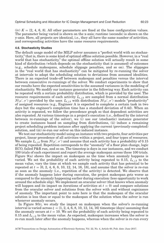
(iv) K = {2, 4, 6, 8}. All other parameters are fixed at the base configuration values.The parameter being varied is shown on the x-axis; runtime (seconds) is shown on they-axis. Here, all projects are identical, i.e., they all have the same number of activities,and corresponding activities have the same resource requirements.

4.6. Stochasticity Studies

The default usage model of the MILP solver assumes a “perfect world with no stochas-ticity,” that is, there is some kind of optimal offline solution possible. However, in a “realworld that has stochasticity,” the optimal offline solution will actually result in somekind of distribution (which depends on the stochasticity that is assumed) of outcomes(e.g., schedule makespans, schedule slippage penalties, and so on). The slippagesin the “real world that has stochasticity” can be mitigated by re-running the solverat intervals to adapt the scheduling solution to deviations from assumed idealities.There is an expected trade-off between makespan and penalties versus the intervalbetween consecutive re-runnings of the solver. We conduct experiments to show thatour results have the expected sensitivities to the assumed variances in the modeling ofstochasticity. We modify our instance generator in the following way. Each activity canbe repeated with a certain probability distribution, which is provided by the user. Theresource requirements of each activity Li, j,k are sampled from a normal distributionN(μ′, σ ′) provided by the user. Li, j,k with distribution N(μ′, σ ′) models “productivity”of assigned resources (e.g., Engineer A is expected to complete a certain task in twodays but the engineer’s completion time has a standard deviation of 0.4d). When anactivity is repeated, we follow the precedence graph so that dependent activities arealso repeated. At various timesteps in a project’s execution (i.e., defined by the intervalbetween re-runnings of the solver), we (i) use our (stochastic) instance generatorto create instances based on sampling from distributions, (ii) induce a remainingproject scheduling problem instance after applying the current (previously-completed)solution, and (iii) re-run our solver on this induced instance.

We test our stochasticity model using an instance with two projects, four activities perproject, linear precedence of all activities within a project, and four types of resources.We sample Li, j,k from N(μ′, σ ′) and assume that each activity has a probability of 0.15of being repeated. Repetition corresponds to the “anomaly” of a floor plan change, logicECO, failed P&R run, and so on. The timestep is days in our instances, and we conduct100 trials of each experiment and report the average makespan across these 100 trials.Figure 9(a) shows the impact on makespan as the time when anomaly happens isvaried. We set the probability of each activity being repeated to 0.15, Li, j,k to themean value, vary the time at which we sample each activity that has potential to berepeated at t = {0, 2, 4, 6, 8, 10, 12, 14, 16, 18}, and assume that the solver is re-runas soon as the anomaly (i.e., repetition of the activity) is detected. We observe thatif the anomaly happens later during execution, the project makespan gets worse ascompared to the anomaly happening earlier during execution (less opportunity to workaround the schedule slip). We implement an oracular solver (that knows when anomalywill happen and its impact on iterations of activities at t = 0) and compare solutionsfrom the oracular solver and solutions from the solver with and without cognizanceof anomaly. The important point to note here is that the makespan of the oracularsolution is less than or equal to the makespan of the solution when the solver is runwhenever anomaly occurs.

In Figure 9(b), we study the impact on makespan when the solver’s re-runninginterval is varied across ξ = {1, 2, 4, 6, 8, 10, 12, 14, 16} timesteps (days) assuming thatthe anomaly occurs at t = 10. We set the probability of each activity being repeated to0.15 and Li, j,k to the mean value. As expected, makespan increases when the solver isre-run much later after the anomaly happens, whereas when the solver is re-run every



Fig. 9. Studies of stochasticity on makespan: (a) time when anomaly happens is varied, (b) interval atwhich the solver is re-run is varied, (c) probability of each activity being repeated is varied, (d) resourcerequirements are varied, and (e) when there is uncertainty in schedule.

day or every 2d or every 10d, the anomaly is detected immediately and there is noimpact on makespan as compared to solutions from the oracular solver. For example,when the solver is run every 8d, anomaly is detected at t = 16 and the makespandiverges from the oracular solution by 3.5d. However, when the solver is run every10d, the anomaly is detected at t = 10 and the makespan is the same as that from theoracular solver. In Figure 9(c), we study sensitivity of the makespan to stochasticityin repeating activities. We vary the probability of each activity being repeated from{0.15, . . . , 0.9} in steps of 0.05. We assume that the anomaly happens at t = 12 (withprobability {0.15, . . . , 0.9}), the solver is re-run every six (or any divisor of 12) days, andset Li, j,k to the mean value. As expected, the makespan increases as the probability ofrepetition increases, and solutions from the oracular solver have a smaller makespancompared to the solutions from the solver that is re-run every 6d. In Figure 9(d), westudy sensitivity of the makespan to stochasticity in resource requirements when theanomaly happens (i.e., we sample resource requirements for remaining activities) att = 10 and the solver is re-run immediately. We sample Li, j,k for activities that arerunning or have not yet started. We vary the standard deviation across +{0, 15, 20,25, 30, 35, 40}% of the mean. We observe that as standard deviation increases (i.e.,resources become less predictable) the average makespan increases. In Figure 9(e), westudy distribution of the makespan when there is uncertainty in the schedule. For agiven problem instance, considering that there are no anomalies, we sample Li, j,k from



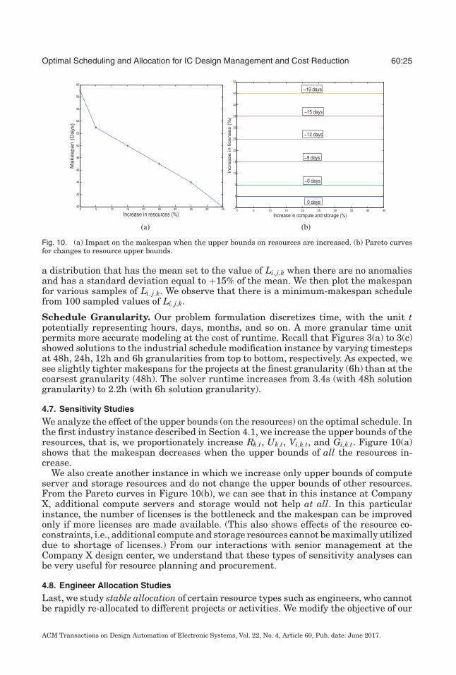
Fig. 10. (a) Impact on the makespan when the upper bounds on resources are increased. (b) Pareto curvesfor changes to resource upper bounds.

a distribution that has the mean set to the value of Li, j,k when there are no anomaliesand has a standard deviation equal to +15% of the mean. We then plot the makespanfor various samples of Li, j,k. We observe that there is a minimum-makespan schedulefrom 100 sampled values of Li, j,k.

Schedule Granularity. Our problem formulation discretizes time, with the unit tpotentially representing hours, days, months, and so on. A more granular time unitpermits more accurate modeling at the cost of runtime. Recall that Figures 3(a) to 3(c)showed solutions to the industrial schedule modification instance by varying timestepsat 48h, 24h, 12h and 6h granularities from top to bottom, respectively. As expected, wesee slightly tighter makespans for the projects at the finest granularity (6h) than at thecoarsest granularity (48h). The solver runtime increases from 3.4s (with 48h solutiongranularity) to 2.2h (with 6h solution granularity).

4.7. Sensitivity Studies

We analyze the effect of the upper bounds (on the resources) on the optimal schedule. Inthe first industry instance described in Section 4.1, we increase the upper bounds of theresources, that is, we proportionately increase Rk,t, Uk,t, Vi,k,t, and Gi,k,t. Figure 10(a)shows that the makespan decreases when the upper bounds of all the resources in-crease.

We also create another instance in which we increase only upper bounds of computeserver and storage resources and do not change the upper bounds of other resources.From the Pareto curves in Figure 10(b), we can see that in this instance at CompanyX, additional compute servers and storage would not help at all. In this particularinstance, the number of licenses is the bottleneck and the makespan can be improvedonly if more licenses are made available. (This also shows effects of the resource co-constraints, i.e., additional compute and storage resources cannot be maximally utilizeddue to shortage of licenses.) From our interactions with senior management at theCompany X design center, we understand that these types of sensitivity analyses canbe very useful for resource planning and procurement.

4.8. Engineer Allocation Studies

Last, we study stable allocation of certain resource types such as engineers, who cannotbe rapidly re-allocated to different projects or activities. We modify the objective of our



Table VIII. Total Cost, Number of Switches, μ and σ of Switches Overall Engineers,and Overall Schedule Makespan Impact

Switching Cost Total μ σ � OverallTest case N # Engineers C # Switches (# Switches) (# Switches) Total Cost Makespan

E1 5 100

0 4108 39.8 7.33 0 0 weeks0.1 3804 38.8 7.20 410.4 +1 weeks1 2180 21.5 6.36 1920 +1 weeks10 1280 12.4 4.28 12840 +1 weeks

100 0 0 0 15050 +4 weeks

E2 10 150

0 5690 37.5 5.25 0 0 weeks0.1 5520 36.6 5.20 572 +1 weeks1 2777 18.5 5.06 3207 +2 weeks10 1550 10.6 3.4 16360 +2 weeks

100 0 0 0 22680 +4 weeks

E3 30 150


100 0 0 0 28500 +4 weeks

E4 30 250


100 0 0 0 251280 +7 weeks

SCM problem as follows.

minimize CK∑

k=1

N∑i=1

J(i)∑j=1

T∑t=2

|ri, j,k,t − ri, j,k,t−1| +N∑

i=1

T∑t=1

C pi (t) +

N∑i=1

J(i)∑j=1

T∑t=1

Cai, j(t) (39)

This optimization is subject to start and finish times, resource upper-bounds andactivity precedence constraints, as described in Section 3.3. We consider each engineeras a resource type; thus, Rk,t = 1,∀t. In consecutive timesteps t − 1 and t, the engineeris either working on an activity ai, j of Project Pi, or working on another activity of thesame project or a different project. When the engineer is working on the same activity,there is no switching between consecutive timesteps and the absolute difference of|ri, j,k,t − ri, j,k,t−1| is zero. However, when the engineer works on a different activity orproject, then the absolute difference is one and is multiplied by the fixed cost C ofswitching activities or projects. The total number of switches made by the engineeris multiplied by C in the objective function to obtain the total cost of switching. Ourobjective is to minimize the cost of switching across all engineers.

To verify this formulation, we use our generator described in Section 4.4 and createfour input instances E1,2,3,4 with 5, 10, 30, and 30 projects, respectively. Each instancehas one activity per project (i.e., J(i) = 1,∀i = 1, . . . , N), and the number of engineersvarying between 100 and 250 (i.e., K = 100, K = 150, or K = 250), T = 90 weeks,Rk,t = Uk,t = 1,∀t, and s(i, 1) = 1. In instance E1, we assess solutions with C set to0, 0.1, 1, 10, and 100. C = 0 corresponds to zero cost of switching between projects,C = 1 corresponds to a small cost of switching, and C = 100 corresponds to a large costof switching. Table VIII summarizes the number of switches made by each engineerover all projects. In instance E1, when the cost of switching is zero, there are a totalof 4108 switches without any impact to the overall schedule makespan. When thecost of switching is large (C = 100), there are zero switches but the overall schedulemakespan increases by 4wk. When the cost of switching is small (C = 1), the totalnumber of switches reduces from 4108 to 2180, but the makespan increases by 1wkand the total cost increases from 0 to 15050. Thus, we observe sensible behavior of the



trade-off between total number of switches (stable assignment) and overall schedulemakespan. Instances E2 and E3 further show the trade-off in total number of switchesand overall schedule makespan using different values of C for the same number ofprojects and engineers. Instance E4 demonstrates scalability as the number of projectsis increased to 30 and the number of engineers is increased to 250. In all instances, wereduce the total number of switches made by engineers by increasing C; however, thetotal cost increases as schedules of projects are pushed out by 1wk to 7wk.20

We also solve a variant of the engineer allocation problem by adding constraintsthat upper-bound the number of switches of each engineer during the overall schedulemakespan. We use the same objective function as the SCM problem with additionalconstraints. We validate our solver for this variant using instance E4 described earlier,and by varying the upper bound on the number of switches allowed per engineer as{+∞, 30, 20, 10, 5, 1}. When the upper bound is +∞, the total cost is zero and matchesthe total cost when C = 0 for instance E4 in Table VIII. When the upper bound is 30,the total cost is 3830; when the upper bound is 20, the total cost is 33150; when theupper bound is 10, the total cost is 97150; when the upper bound is 5, the total cost is116650; and when the upper bound is 1, the total cost is 226250.

5. CONCLUSIONS AND FUTURE WORK

The lack of tools for management of semiconductor design resources (servers, tool li-censes, engineering headcount) can impact a company’s bottom line by many millionsof dollars per year. In this work, we capture multi-project, multi-resource constrainedproject scheduling as SCM and RCM MILP formulations that are readily solvable us-ing commercial engines such as CPLEX. The MILP solutions provide optimal schedul-ing and allocation solutions for complex multi-tapeout management scenarios in alarge design center. Aspects of our formulation that are unique to semiconductor de-sign, and that take our work beyond the earlier RCPSP formulation of Kolisch andHartmann [1999], Kolisch et al. [1992], and Kolisch and Sprecher [1996], include mul-tiple resource pools and co-constraints between resources of different types. We demon-strate the flexibility and value of our optimization in three scenarios taken from therecent history of Company X’s design center. (1) We find an optimal schedule for threeconcurrent tapeouts when a late-breaking RTL change hits one of the projects, andsave 1.4 work-weeks of schedule compared to the solution deployed by the company.This level of saving corresponds to 2.7% of annual labor and infrastructure costs andenhances market competitiveness. (2) We find an optimal schedule for 20+ projects,subject to datacenter capacity limits and a tethering constraint with respect to originalforecast resource allocations. Our solution shows that a slight relaxation of the tether-ing constraint would allow committed projects to proceed within resource limits. Oursolution meets the schedule with no additional servers. By contrast, in the absence ofdecision support tools, the company’s solution entailed the purchase of hundreds of ad-ditional servers. (3) We find an optimal allocation of human resources for four projectsand save up to 37% of a particular resource type relative to the solution adopted bythe company. In a non-US location, this single-resource type reduction would imply a∼$3.7M savings for the company within a half-year project scheduling makespan. Wealso provide “what-if” analyses capabilities with our solver and demonstrate sensitiv-ity analyses (schedule benefits of incremental resources) and scalability of our solutionapproach. Since we introduce new concepts such as conditionally-shared, segregated,

20Instance E1 has ∼46K variables, ∼350K constraints, and a runtime of around 3min. Instance E2 has∼150K variables, ∼1.1M constraints, and a runtime of around 28min. Instance E3 has ∼450K variables,∼3.2M constraints, and a runtime of around 50min. Instance E4 has ∼680K variables, ∼5.4M constraints,and a runtime of around 2.3h.



and fully-shared resource types along with resource co-constraints, we are unable tocompare against any previously existing MILP formulations of such problems. Using a(stochastic) instance generator, we demonstrate impact on makespan with stochasticityin resource requirements and iterations in activities.

Our work is applicable across multiple stages of project and capacity planning pro-cesses. For example, it can be used (i) as part of a fiscal planning process to comprehendthe overall resource requirements of a site or a computing cluster, (ii) by program man-agement as a what-if tool so that infrastructure can join engineering headcount as afactor in scheduling decisions, and (iii) by “Engineering Compute” operations teamsto understand the impact of product roadmap or schedule changes on datacenter andEDA licensing infrastructure so that corrective actions may be taken in a proactiveand principled manner. By providing a foundation for improved engineering resourceallocation to maintain high overall resource utilizations and low schedule latencies, weenable design organizations to improve design throughput and efficiency with givenresources. Ultimately, this helps to continue the scaling of design cost efficiencies thatare so vital to the IC industry. Our solving of instances with co-constraints, stabilityconstraints and tethering forecast resource allocations may be of interest in other ap-plication domains, such as industrial assembly (e.g., automobile assembly), air trafficmanagement, and workflow scheduling in grid computing [Laborie and Godard 2007].

Our formulations can be improved in a number of directions that are the subject ofongoing investigation. For instance, it will be helpful to be able to automatically deter-mine threshold values of inputs (e.g., the schedule length T or the tethering constraintδ) at which feasible solutions exist. Scheduling decisions should also comprehend dis-tributions of job sizes or job complexities (which can vary per block and according to thestate of a project), and automatic change of timestamps when schedule changes occur.Solutions can be further stabilized by adopting iterative optimization approaches. Afurther open direction is to optimize robustness of scheduling solutions in the face ofstochasticity in resources and personnel.

APPENDIX

Table IX maps activities and resources from problem instances in Section 4.1 andSection 4.3 to chip design flow terminologies.

Table IX. Glossary for the Schedule Modification Use Case (Section 4.1) and (Human)Resource Allocation Use Case (Section 4.3)

Schedule modification use case (Section 4.1) Human resource allocation use case (Section 4.3)Activity / Resource Chip Design Flow Mapping Activity / Resource Chip Design Flow Mapping

A1 Placement A12 Block-Level Design (BLD)A2 Routing A13 Full-Chip Design (FCD)A3 Search and Repair A14 Block-Level Verification (BLV)A4 Extraction A15 Full-Chip Verification (FCV)A5 Static Timing Analysis (STA) A16 Block-Level Physical Design (BLPD)A6 Functional ECO A17 Full-Chip Physical Design (FCPD)A7 Extraction A18 Gate-Level Simulation (GLS)A8 STA (per corner) A19 Emulation (EMU)A9 Timing ECO HR1 Design ResourcesA10 Extraction HR2 Design Verification ResourcesA11 STA (per corner) HR3 PD ResourcesL1 P&R License HR4 EMU ResourcesL2 RCX License – –L3 STA License – –



REFERENCES

P. Agrawal, B. Chatterjee, A. B. Kahng, P. K. Myana, and S. Nath. 2015. Optimal multi-tapeout projectscheduling for enterprise-scale design management and cost reduction. Work-in-Progress, DAC.

M. Ayala and C. Artigues. 2010. On Integer Linear Programming Formulations for the Resource-ConstrainedModulo Scheduling Problem, Rapport LAAS. Technical Report 10393.

P. Baptiste and S. Demassey. 2004. Tight LP bounds for resource constrained project scheduling. OperationsResearch Spectrum 26, 251–262.

D. Bienstock and M. Zuckerberg. 2009. A new LP algorithm for precedence constrained production scheduling.Optimization Online 1–33.

A. Bonfietti, M. Lombardi, L. Benini, and M. Milano. 2014. Cross cyclic resource-constrained schedulingsolver. Artificial Intelligence 206, 25–52.

W.-T. J. Chan, A. B. Kahng, S. Nath, and I. Yamamoto. 2014. The ITRS MPU and SOC system drivers:Calibration and implications for design-based equivalent scaling in the roadmap. In Proceedings of theIEEE International Conference on Computer Design. 153–160.

N. Christofides, R. Alvarez-Valdes, and J. M. Tamarit. 1987. Project scheduling with resource constraints: Abranch and bound approach. European Journal of Operational Research 29, 262–273.

S. Fenstermaker, D. George, A. B. Kahng, S. Mantik, and B. Thielges. 2000. METRICS: A system architecturefor design process optimization. In Proceedings of the ACM/IEEE Design Automation Conference. 705–710.

R. Friese, T. Brinks, C. Oliver, H. J. Siegel, and A. A. Maciejewski. 2012. Analyzing the trade-offs betweenminimizing makespan and minimizing energy consumption in a heterogeneous resource allocation prob-lem. In Proceedings of International Conference on Advanced Communications and Computation. 81–89.

A. B. Kahng and G. Smith. 2002. A new design cost model for the 2001 ITRS. In Proceedings of InternationalSymposium on Quality Electronic Design. 190–193.

B. Keller and G. Bayraksan. 2009. Scheduling jobs sharing multiple resources under uncertainty: A stochasticprogramming approach. IIE Transactions 42, 16–30.

R. Kolisch and S. Hartmann. 1999. Heuristic algorithms for the resource-constrained project schedulingproblem: Classification and computational analysis. International Series in Operations Research & Man-agement Science 14, 147–178.

R. Kolisch and A. Sprecher. 1996. PSPLIB – A project scheduling problem library. European Journal ofOperational Research 96, 205–216.

R. Kolisch, A. Sprecher, and A. Drexl. 1992. Characterization and generation of a general class of resource-constrained project scheduling problems. Management Science 41, 10, 1693–1703.

B. A. Kramer and C. L. Hwang. 1991. Resource constrained project scheduling: modeling with multiplealternatives. Mathematical and Computational Modeling 15, 8, 49–63.

P. Laborie and D. Godard. 2007. Self-adapting large neighborhood search: Application to single-mode schedul-ing problems. Multidisciplinary International Scheduling Conference, 276–284.

M. Li, Y. Zhang, W. Jiang, and J. Xie. 2009. A particle swarm optimization algorithm with crossover forresource constrained project scheduling problem. In Proceedings of International Conference on ServicesScience, Management and Engineering. 69–72.

Y. Li, J. Han, and W. Zhou. 2014. Cress: Dynamic scheduling for resource constrained jobs. In Proceedings ofInternational Conference on Computational Science and Engineering. 1945–1952.

S. Mohanty and M. K. Nayak. 2011. Optimization model in human resource management for job allocationin ICT project. International Journal of the Computer, the Internet and Management 19, 3, 21–27.

R. H. Mohring, A. S. Schulz, F. Stork, and M. Uetz. 2001. On project scheduling with irregular starting timecosts. Operations Research Letters 28, 149–154.

Qualcomm Inc. (IT project manager). 2014. Personal Communication.Z. Qiong, G. Yichao, Z. Ging, Z. Jie, and C. Xuefang. 2010. An ant colony optimization model for parallel

machine scheduling with human resource constraints. In Proceedings of International Conference onDigital Enterprise Technology Advances in Intelligent and Soft Computing, Vol. 66. 917–926.

F. Salewski, A. Schirmer, and A. Drexl. 1997. Project scheduling under resource and mode identity con-straints: Model, complexity, methods, and application. European Journal of Operational Research 102,1, 88–110.

G. Smith. 2014. Personal Communication.G. Smith. 2014. Updates of the ITRS design cost and power models. In Proceedings of the IEEE International

Conference on Computer Design. 161–165.



F. B. Talbot. 1982. Resource-constrained project scheduling with time-resource tradeoffs: The nonpreemptivecase. Management Science 28, 10, 1197–1210.

Cadence Assura QRC. Retrieved July 04, 2016 from https://www.cadence.com/content/cadence-www/global/enUS/home/tools/digital-design-and-signoff.html.

Cadence Innovus Implementation System. Retrieved July 4, 2016 from https://www.cadence.com/content/cadence-www/global/en US/home/tools/digital-design-and-signoff.html.

Cadence Tempus Timing Signoff. Retrieved July 4, 2016 from https://www.cadence.com/content/cadence-www/global/en US/home/tools/digital-design-and-signoff.html.

Dassault Systems Enovia Synchronicity. Retrieved July 8, 2016 from http://www.3ds.com/products-services/enovia/products/v6/synchronicity-designsync/.

Glassdoor. Retrieved January 1, 2017 from https://www.glassdoor.com/Salaries/index.htm.How Green is my Silicon Valley? Retrieved July 4, 2016 from http://dac.com/sites/default/files/DACArchive/

pubs/46DACFinal Prgm.pdf.IBM ILOG CPLEX. Retrieved July 4, 2016 from http://www-03.ibm.com/software/products/en/

ibmilogcpleoptistud/.IC Manage. Retrieved July 8, 2016 from https://www.icmanage.com/ic-design-management-best-practices/.inMotion Creative Project Management. Retrieved July 4, 2016 from http://explore.inmotionnow.

com/capterra-project-management.ITRS. Retrieved July 4, 2016 from http://www.itrs2.net/.Nefelus Design Tools. Retrieved July 8, 2016 from http://www.nefelus.com/design-tools/.UCSD Design Cost Optimization Solver for Multi-Tapeout Project Scheduling. Retrieved July 4, 2016 from

http://vlsicad.ucsd.edu/MILP/.When The Chips are Down. Retrieved July 4, 2016 from http://qz.com/387490/as-moores-law-turns-50-

computer-chips-continue-to-get-cheaper-and-more-powerful/.Platform Load Sharing Facility. Retrieved July 4, 2016 from http://www-03.ibm.com/systems/services/

platformcomputing/lsf.html.PSLIB Data Sets. Retrieved July 4, 2016 from http://www.om-db.wi.tum.de/psplib/download.html.Runtime Design Automation. Retrieved July 4, 2016 from http://www.rtda.com/.Qualcomm Snapdragon. Retrieved July 4, 2016 from https://www.qualcomm.com/products/snapdragon.Salesforce Project Management. Retrieved July 8, 2016 from https://www.salesforce.com/.Samsung Exynos. Retrieved July 4, 2016 from http://www.samsung.com/semiconductor/products/exynos-

solution/application-processor/.Synopsys IC Compiler. Retrieved July 4, 2016 from http://www.synopsys.com/Tools/Implementation/

PhysicalImplementation/Pages/default.aspx.Synopsys PrimeTime. Retrieved July 4, 2016 from http://www.synopsys.com/Tools/Implementation/SignOff/

Pages/PrimeTime.aspx.Synopsys Star-RCXT. Retrieved July 4, 2016 from http://www.synopsys.com/Tools/Implementation/SignOff/

Pages/StarRC-ds.aspx.

Received July 2016; revised November 2016; accepted December 2016


https://www.cadence.com/content/cadence-www/global/en ignorespaces US/home/tools/digital-design-and-signoff.html

https://www.cadence.com/content/cadence-www/global/en ignorespaces US/home/tools/digital-design-and-signoff.html

https://www.cadence.com/content/cadence-www/global/en US/home/tools/digital-design-and-signoff.html




http://www.3ds.com/products-services/enovia/products/v6/synchronicity-designsync/

http://www.3ds.com/products-services/enovia/products/v6/synchronicity-designsync/

https://www.glassdoor.com/Salaries/index.htm

http://dac.com/sites/default/files/DACArchive/pubs/46DACFinal Prgm.pdf

http://dac.com/sites/default/files/DACArchive/pubs/46DACFinal Prgm.pdf

http://www-03.ibm.com/software/products/en/ibmilogcpleoptistud/

http://www-03.ibm.com/software/products/en/ibmilogcpleoptistud/

https://www.icmanage.com/ic-design-management-best-practices/

http://explore.inmotionnow.com/capterra-project-management

http://explore.inmotionnow.com/capterra-project-management

http://www.itrs2.net/

http://www.nefelus.com/design-tools/

http://vlsicad.ucsd.edu/MILP/

http://qz.com/387490/as-moores-law-turns-50-computer-chips-continue-to-get-cheaper-and-more-powerful/

http://qz.com/387490/as-moores-law-turns-50-computer-chips-continue-to-get-cheaper-and-more-powerful/

http://www-03.ibm.com/systems/services/platformcomputing/lsf.html

http://www-03.ibm.com/systems/services/platformcomputing/lsf.html

http://www.om-db.wi.tum.de/psplib/download.html

http://www.rtda.com/

https://www.qualcomm.com/products/snapdragon

https://www.salesforce.com/

http://www.samsung.com/semiconductor/products/exynos-solution/application-processor/

http://www.samsung.com/semiconductor/products/exynos-solution/application-processor/

http://www.synopsys.com/Tools/Implementation/PhysicalImplementation/Pages/default.aspx

http://www.synopsys.com/Tools/Implementation/PhysicalImplementation/Pages/default.aspx

http://www.synopsys.com/Tools/Implementation/SignOff/Pages/PrimeTime.aspx

http://www.synopsys.com/Tools/Implementation/SignOff/Pages/PrimeTime.aspx

http://www.synopsys.com/Tools/Implementation/SignOff/Pages/StarRC-ds.aspx

http://www.synopsys.com/Tools/Implementation/SignOff/Pages/StarRC-ds.aspx

Optimal Scheduling and Allocation for IC Design … · Optimal Scheduling and Allocation for IC...

Documents

Transcript of Optimal Scheduling and Allocation for IC Design … · Optimal Scheduling and Allocation for IC...