DIVISION OF BUILDING MATERIALSLUND INSTITUTE OF TECHNOLOGY

/v

CRACK GROWTH AND DEVELOPMENT OF FRACTURE ZONES INPLAIN CONCRETE AND SIMILARMATERIALSPER-ERIK PETERSSON

REPORT TVBM-1006LUND SWEDEN 1981

CRACK GROWTH AND DEVELOPMENT OF FRACTURE ZONESIN PLAIN CONCRETE AND SIMILAR MATERIALS

av Per-Erik Petersson

civ. ing. Hid.

AKADEMISK AVHANDLING

som för avläggande av teknologie doktorsexamenvid tekniska fakulteten vid universitetet iLund kommer att offentligen försvaras vid sek-tionen för Väg och Vatten, John Ericssons väg 1,sal V:A, fredagen den 4 december 1981, kl 13.15.

OrganiriiionLl'ND UNIVERSITY

Division of Building MaterialsLund Institute of TechnologyP 0 Box 725S-220 07 LUND Sweden

Document nimeDOCTORAL DISSERTATION

Date of issue

December 1981COPEN IUTVDG/(1VBM-1OO6)/1-174/(1981)

Author)*)

Per-Erik PeterssonSponsoring organizationNational Swedish Board for Technicalvelopment

De-

Title and subtitle

Crack growth and development of fracture zones in plain concrete and similar materials

Abstract

A calculation model (the Fictitious Crack Model), based on fracture mechanics and thefinite element method, 1s presented. In the model the fracture zone in front of acrack is represented by a fictitious crack that 1s able to transfer stress. The stresstransferring capability of the fictitious crack normally decreases when the crackwidth increases.The applicability of linear elastic fracture mechanics to concrete and similar mate-rials is analysed by use of the Fictitious Crack Model. It" Is found that linear elas-tic fracture mechanics 1s too dependent on, among other things, specimen dimensions tobe useful as a fracture approach, unless the dimensions, for concrete structures, arein order of meters. The usefulness of the J-integral, the COD-approach and the R-curveanalysis is also found to be very limited where cementitious materials are concerned.

The complete tensile stress-strain curve is introduced as a fracture mechanical para-meter. The curve can be approximatively determined if the tensile strength, theYoung's modi1us and the fracture energy are known. Su1table~lest methods Tor determi-ning" TRise~~/'Voerties are presented and test results are reported for a number of con-crete qua! » a.

A new tyr * very stiff tensile testing machine Is presented by which it is possibleto carry r . itable tensile tests on concrete. The complete tensile stress-straincurves h •«• feen determined for a number of concrete qualities.The thesi' overs a complete system for analysing crack propagation in concrete as itInclude* -ealistic material model, a functional calculation model and methods fordetermiv" «/ the material properties necessary for the calculations. Therefore thiswork oi r t to be of use as a base for further studies of the fracture process of con-crete < i similar materials.

Keywords

fracture mechanics, cracking, concrete,finite element method, fracture zone, tensilestress-.» rain curve, tensile strength, fracture energy, test methods

Classificat- <i system and/or index terms (if any)

Supplementary bibliographical information

English

ISSN and kev tide

ISSN 0349-4985 Crack growth and development of fracture zones....ISBN

Recipient's notes Number ol pages185pp.

Price65 kr

Securitv clauifioiion

and address)D1y o f B u l l d | n g Materials, Lund Inst i tute of Technology

P 0 Box 725, S-220 07 Lund, Sweden

I. the undersigned, being (he copyright owner of the abstract of the above-mentioned dissertation, hrrebv grant to allreference sources permission to publish and disseminate the abstract of (he above-mentioned disser(alii;n.

Signature. ,1981-11-05

CODEN: LUTVDG/lTVBM--1006//1 - 174/(1981)

CRACK GROWTH AND DEVELOPMENT OF FRACTURE ZONES INPLAIN CONCRETE AND SIMILARMATERIALSPER-ERIK PETERSSON

ISSN 0349-4985

PREFACE

This work has been carried out at the Division of Bui 1dinq Materials at the

Lund Institute of Technology in Sweden. The project was financiallv s,.ppor-

ted by grants from the Swedish Board for Technical Development.

All the members of the staff at the Division of Building Materials have,

more or less, contributed to the performance of this project and the author

wants to express his thanks to them all and especially to

Professor Arne Hillerborg for his encouragement and his experien-

ced and clever guidance in planning and carrying cx.t the project.

Leif Erlandsson for his invaluable help during the development

of new testing equipment.

Bo Johansson for his skill and efficiency when carrying out the

tests.

Britt Andersson (drawing) and Anni-Britt Nilsson (typing) for

their interest and ability in producing a good result.

Lund, October 1981

Per-Erik Petersson

CONTENTS

PREFACE I

CONTENTS III

LIST OF SYMBOLS V

SUMMARY VII

1 INTRODUCTION 1

2 FRACTURE MECHANICS 3

2.1 Introduction 3

2.2 Linear elastic fracture mechanics 42.2.1 Energy criterion 42.2.2 Stress intensity criterion 52.2.3 Cohesive zones 7

2.3 Elastic-plastic fracture mechanics 72.3.1 Introduction 72.3.2 The Dugdale model 92.3.3 The J-integral 102.3.4 The crack opening displacement (COD) 102.3.5 R-curve analysis 10

2.4 Fracture mechanical models considering the influence ofthe fracture zone 13

3 THE FICTITIOUS CRACK MODEL 15

3.1 The tensile fracture of concrete 15

3.2 The Fictitious Crack Model and its applicability 19

4 THE FINITE ELEMENT METHOD APPLIED TO THE FICTITIOUS CRACK MODEL 23

4.1 Introduction 23

4.2 Calculation method I: substructure 23

4.3 Calculation method II: the super position principle 32

4.4 Element wide fracture zones 34

4.5 Material parameters affecting the choice of the finiteelement mesh /

5 THE FRACTURE ZONE 43

5.1 The width of the fracture zone 43

5.2 The development of the fracture zone 47

- I V -

6 THE FICTITIOUS CRACK MODEL vs OTHER APPROACHES 55

6.1 Introduction 55

6.2 Linear elastic fracture mechanics 596.2.1 Notch sensitivity 596.2.2 K - and G -approaches 67

6.3 The J-integral approach 77

6.4 The crack opening displacement approach 88

6.5 R-curve analysis 90

6.6 Conclusions 98

7 APPROXIMATIVE DETERMINATION OF THE •-• AND j-w CURVES 101

7.1 Introduction 101

7.2 Determination of the tensile strength (f.) on prismaticspecimens 1017.2.1 Introduction 1J17.2.2 Direct tensile tests on prismatic specimens 104

7.3 Determination of the Young's modulus (E) 107

7.4 Determination of the fracture energy (Gp) 1097.4.1 Introduction 1097.4.2 Stability conditions for three-point bend tests on

notched beams 1107.4.3 Evaluation of the Gp-test 1157.4.4 Gp as a material property 1237.4.5 Suitable specimen dimensions for the Gp-test 132

7.5 Experimental investigation of the fracture mechanical pro-perties of concrete 1347.5.1 Testing procedure 1347.5.2 Materials and mix proportions 1387.5.3 Preparation of specimens 1407.5.4 Results 1407.5.5 Discussion 140

DETERMINATION OF THE a-w CURVE FROM STABLE STRESS-DEFORMATIONCURVES 151

8.1 Introduction 151

8.2 Stability conditions for the direct tensile test 153

8.3 A stiff testing machine for stable tensile tests on concre-te and similar materials 157

8.4 Experimental determination of the T-W curve for concrete 1618.4.1 Testing procedure 1618.4.2 Materials and mix proportions 1638.4.3 Preparation of specimens 1638.4.4 Results and discussion 163

9 REFERENCES 171

- v -

LIST

Aa

b

COD

d

dF

E

EdF

Fcffc

ff

fJetGGcGFJ

JcK

KcKRk

i

OF SYMBOLS

area

crack depth and notch depth

width

crack opening displacement

depth

depth of the fracture zone

ligament depth

Young's modulus

dynamic Young's modulus

load

fracture load

resonance frequency

compression strength

flexural tensile strength

tensile strength

net flexural tensile strength

strain energy release rate

critical strain energy release rate

fracture energy

value of the J-integral

critical value of the J-integral

stress intensity factor

critical stress intensity factor

resistance to crack growth

stiffness

length

£ch characteristic length Uch=GpE/f^)

i gauge length

M moment

M mass

m mass per unit length

P force

Q energy

U energy

W /C water-cement ratio

w width of the fictitious crack

w critical value of the width of the fictitious crack

- V I -

Y

6

e

emV

a

acayJ

°s

surface energydeformation or displacementstrainmean strain

Poisson's ratio

stress

critical stressyield stress

shrinkage stress

- V I I -

SUMMARY

When a notched specimen of a linear elastic material becomes subjected to

load, the region in front of the notch tip will be highly stressed. A real

material cannot stand these high stresses and a damage zone will develop

in front of the notch tip. For concrete and other non-yielding materials,

the damage zone is caused by the development of micro-cracks. The material

in this micro-cracked material volume, or /;•.;.'••<;•-. :;•>:• , is partly destroyed

but is still able to transfer stress. The stress transferring capablity

normally decreases when the local deformation of the zone increases, i.e.

when the number of micro-cracks increases. This thesis deals with the

'jeloprcnt of fracture ::on,;c and how the fracture zones affect the •.••.••••• .•• -

apatien and the ''raoiuv, * > c , . v for :'.:'>. ••:'.••. -. and similar materials.

In the calculation model presented here, the fracture zone is modelled by

a crack that is able to transfer stress and the stress transferring capa-

bility depends on the width of the crack in the stressed direction (sec-

Fig 3.6). As the stress transferring crack is not a real crack but a ficti-

tious crack, the model is called the •'',•• '•'-..• ';•.•••• " '. In the calcu-

lations the fictitious crack (i.e. the fracture zone) is assumed to start

developing at one point when the first principal stress reaches the tensile

strength and the fictitious crack develops perpendicular to the first prin-

cipal stress. The deformation properties are given by two relations; one re-

lation between the stress and the relative strain, i.e. a •-• ••••• , for the

material outside the fictitious crack and one relation between the stress

and the opening of the fictitious crack, i.e. a •-.• •-.-• (see Fiq 3.4;.

These curves are considered as material properties and they are, together

with Poisson's ratio, the only parameters necessary to know when carryinq

out calculations by using the Fictitious Crack Model.

The Fictitious Crack Model cannot normally be treated analytically but nu-

merical methods have to be used. In this thesis calculation methods are pre-

sented which are based on the /"• '• . ' ••• •• • • •' .

A number of calculations have been carried out by using the Fictitious Crack

Model and the results seem to be in good agreement with experimental results

(cf Tables 6:1 and 6:3, Fig:s 6.33, 6.35, 7.1 and 8.16).

Calculation results are presented which indicate that up to 150 mm long

fracture zones develop in front of notches in concrete structures (see

- VIII -

Fig 5.6). These results are in good agreement with test results presented

in literature.

The applicability of linear elastic fracture mechanics to concrete and simi-

lar materials is analysed by use of the Fictitious Crack Model. It is found

that linear elastic fracture mechanics is too dependent on, among other

things, specimen dimensions to be useful as a fracture approach, unless the

dimensions, for concrete structures, are in order of meters. The usefulness

of the J-integral, the Crack Opening Displacement-approach and the R-curve

analysis is also found to be very limited where cementitious materials are

concerned.

The c-e and c-w curves can be approximately determined if the t^r.a:'.--

sti'.:r.:jth ( f t ) , the Young's roduluc (E) and the ??•::? tuvc -:*:ci>ji. (G,-) are

known (see Fig 4.10). Gp is defined as the amount of energy necessary to

create one unit of area of a crack and consequently Gp equals the area un-

der the j-w curve. Gp can be determined by use of a st^blr three-point bend

test on a notched beam and this test method is dealt with in detail. Among

other things, the stability conditions for the three-point bend test are gi-

ven and test results are presented which imply that Gp is suitable for use

as a material property for concrete. The direct tensile test is also dealt

with and a new type of clamping grips is presented, which can be used for

determination of the tensile strength on prismatic concrete specimens (cee

Fig 7.3)

Test results of f., E and Gp are presented for a number of concrete quali-

ties (see Fig:s 7.31-7.35). Gp normally appears to be 70-140 N/m and is

especially dependent on the quality of aggregate, water-cement-ratio and age.

The a-w curve can be directly determined from the .•' rr", tensile stress-

strain curve and in the last Chapter a new type of very stiff terting ma-

chine is presented by which it is possible to carry out stable tensile tests

on concrete (see Fig 8.5). The complete stress-deformation curves, and thus

the o-w curves, have been determined for a number of concrete qualities (see

Fig:s 8.10-8.13). It was found that the shapes of the a-w curves are similar

for the different concrete qualities. A result of this is that no "compli-

cated" stable tensile tests have to be carried out in order to determine

a-w curves for concrete but good approximations of the curves can be deter-

mined by use of the "simple" f.- and Gp-tests. Furthermore, due to the small

variations of the shapes of the a-w curves for concrete, the fracture pro-

- I X -

p e r t i e s c a n b e e x p r e s s e d b y a s i n g l e p a r a m e t e r c a l l e d t h e •• ••••

'•.•:.r•'•• (••c\?1 V h 1S de<"ined a s G p ^ ; / f t " a n d t h e s n a l l o r t h e v a l u e c.f ,.n

t h e m o r e " b r i t t l e " t h e m a t e r i a l i s . F o r m o s t c o n c r e t e q u a l i t i e s ,., ^ee"

t o b e 2 0 0 - 4 0 0 m m .

T h e d e s c r i p t i o n a b o v e c o v e r s a c o m p l e t e s y s t e m f o r a n a l y : i'": i.ru> :;'••;>:

t i o n in c o n c r e t e as it i n c l u d e s a r e a l i s t i c m a t e r i a l m o d e l , a f jr.*. t:<>ra"

c u l a t i o n m o d e l a n d m e t h o d s f o r d e t e r m i n i n g the m a t e r i a l paramo*»"'-" n•_•<>_••

f o r t h e c a l c u l a t i o n s . T h e r e f o r e t h i s w o r k o u g h t to be o f uc-e v. A b i , - •

f u r t h e r s t u d i e s o f the f r a c t u r e p r o c e s s o f c o n c r e t e a n d s i m i l a r m a t e r i a '

-1-

1 INTRODUCTION

In the field of fracture mechanics stresses and strains around crack tips in

loaded structu:es are analysed. The fracture of non-yielding materials is a l -

ways caused by crack propagation and therefore it was logical when Kaplan

(1961) started to study the fracture process of concrete by means of fractu-

re mechanics. Since then numereous reports have been published about crack

stability, crack propagation, fracture mechanical test methods and so on for

concrete and similar materials. Almost all of tnese publications have one

t h i n g in c o m m o n ; c o n c r e t e is t r e a t e d as a l i n e a r e l a s t i c m a t e r i a l a n d the w e l l -

known K- and G-approaches, more or less modified, are used. A few researches

have used other methods such as the J-integral approach and R-curve a lysis.

The results of all these efforts are discouraging; in fact, to date there exist

no working fracture mechanical calculation models for c o n c r e t e , no well defi-

ned fracture mechanical material parameters, no well established test methods

and so on. This has given rise to some doubt regarding the usefulness of frac-

ture mechanics when applied to concrete. However, the fracture of concrete is

caused by cracks and consequently it is necessary to use fracture mechanics

when describing the fracture process of concrete but one has to be aware of

the fact that fracture mechanics is not the same as linear elastic 'Yacture

mechanics. As linear elastic fracture mechanics seems unsuitable for concrete

it is consequently necessary to develop approaches that take material »roper-

ties other than the linear elastic ones into c o n s i d e r a t i o n , especially the

properties of the highly strained region in front of the crack tip. Sjch an

approach is presented in this thesis.

The work presented in this report is a part of a research progra- jimed at

developing a fracture mechanical model suitable for analysing the micro- and

macr o - f r a c t u r e of plain and reinforced concrete and similar material'.. In con-

nection with this research program a number of papers have been published,

for example Hillerborg, Modéer and Petersson ( 1 9 7 6 ) , Modéer ( 1 9 7 9 ) , Petersson

(1980a, 1980b, 1 9 8 0 c ) , Petersson and Gustafsson ( 1 9 3 0 ) , Hillerborq (19;:::),

Hillerborg and Petersson ( 1 9 8 1 ) .

This report deals with the macro-fracture of plain concrete and similar m a t e -

rials. The physical properties of the fracture zone in front of a cr<tck t i:, in

a stressed material are discussed and a calculation model is presented by

which the crack growth and the development wf local fracture /ones c cm be ana-

lysed. The calculation model can however be used cor fiuanti tat i ve <•-,* i ma' io' s

only if a number of essential material parameters 4re known, for this •••w,y<;

-2-

the work, to a large extent, is concentrated on the development of suitable

methods for determining the fracture mechanical properties of cementitious

materials and such properties are also presented for a number of qualities

of plain concrete.

This project has, as all other projects, a number of limitations of which

someare 1 isted and discussed below.

a) Concrete is a composite material where the components are cement

paste, aggregate particles and pores but in the calculations con-

crete and other cementitious materials are assumed to be homogeneous

and isotropic. This ought to be a fair assumption when the dimensions

of the structure exceed the dimensions of the largest irregularities

ir. the material by a few times.

b) In the calculations only the development of a single crack (opening

mode) is analysed but in principle the model can also be used when

two or rrore cracks develop simultaneously.

c) For a yielding material plastic deformations take place close to the

crack tip and so called shear lips develop. Due to these plastic de-

formations the fracture mechanical properties of yielding materials

are strongly affected by the state of stress; plane stress or plane

strain. For non-yielding materials the irreversible deformations are

due to the formation of micro-cracks and therefore no plastic de-

formations take place and the difference between plane stress and

plane strain is small. In the calculations presented in this report

plane stress is used and Poisson's ratio (v) is assumed to be 0.2.

d) Most of the calculations and tests are relevant for wet specimens,

i.e. the effect of shrinkage stresses is not dealt with, although

this can be done with the model, see 4.2.

-3-

2 FRACTURE MECHANICS

2.1 Introduction

The reference list in this Chapter is incomplete. However, most of the defini-

tions and expressions are well known in the field of fracture mechanics and

can be found, for example, in Knott (1973) and Carlsson (1976).

Fig 2.1 illustrates an infinitely large plate of linear elastic material and

the plate is subjected to a uniform tensile stress c0 . The stress distribution

will be disturbed if there is a circular hole in the plate. At the most criti-

cal point of the boundary of the hole, the stress will, independently of the

size of the hole, reach three times the applied stress. This means that holes

or other irregularities will considerably reduce the strength of a material.

0 o i i i k i i t k i i i k

,*Ö m. oowhen b »O

Fig 2.1 The stress distributions close to a circular hole, an ellipticalhole and a crack in an infinitely large plate subjected to theuniform stress o .

If the circular hole is replaced by an elliptical hole, the stress at the tip

of the elliptical hole becomes 1 + 2a/b times the applied stress, where a

and b are the major and minor axes of the ellipse respectively. If the minor

axis is much smaller than the major axis, i.e. b << a, then the elliptical

hole is a crack and the stress at the crack tip grows unlimitedly as the ratio

a/b approaches infinity. This means that ordinary stress criterions cannot be

used in this case as the material would then fail as soon as it became subjec-

ted to load,

A material always contains irregularities. However, a real material is never

perfectly linear elastic, at least not at high stresses, and crack tips are

never infinitely sharp and these are the reasons why materials can exist at all.

2.2 Linear el as tic fracture mechanics

2.2.1 Energy criterion

Even if materials never behave perfectly linear elastic it is sometimes possib-

le to approximate the material behaviour with a linear elastic model. As stress

criterions cannot be used, one has to use so called fracture mechanics approa-

ches. The first approach of this type was proposed by Griffith (1921).

Fig 2.2 shows an infinitely large plate subjected to a uniform tensile stress

c . The plate contains a 2a long crack, which is oriented perpendicular to

the applied stress. By equating the elastic strain energy that is released

when the crack advances a small distance ..a at each crack tip and the energy

necessary to create the new crack surfaces, Griffith found an expression for

the critical stress (a ) at which the crack propagates:

where E is the Young's modulus and f is the surface energy per unit area, a is

1 for plane stress and y1/(1-v^) for plane strain, where v is Poisson's ratio.

For concrete v is normally less than 0.2, which means that 1 < .* < 1.02. The

discrepancy between plane stress and plane strain is so small for concrete

that it can be neglected and below all the relations are relevant for plane

stress, i.e. «=1.

By introducing the critical strain energy release rate (G ), (2:1) can be ex-

tended to be relevant also for materials where small, irreversible deforma-

tions take place cl_qse to the crack tip. G includes not only 2> but also the

-5-

Fig 2.2 An infinitely large plate with a 2a long crack oriented :>orcular to the applied stress -Q.

energy consumption due to plastic deformations close to the o w J * i;

(2:1) becomes:

Normally (2:2) is seen as:

G = G.

and G, the strain energy release rate is defined ac

: -+ ;

w h e r e g is a c o r r e c t i o n f a c t o r d e p e n d e n t on t h e s p e c i m e n geome'.ry a n d M,,.

d i n g c a s e , g e q u a l s u n i t y f o r t h e i n f i n i t e l y l a r g e p l a t e in F i g /..-'.

2 . 2 . 2 S t r e s s i n t e n s i t y c r i t e r i o n

T h e s t r e s s d i s t r i b u t i o n in f r o n t o f a c r a c k t i p , u e r p e n d i c u l a r to t h e c r a c

a n d o n a l i n e p a r a l l e l w i t h t h e c r a c k , s e e F i g 2 . 3 , c a n h e e x p r e s s e d a s :

-K +

w h e r e x is t h e d i s t a n c e f r o m t h e c r a c k t i p a n d K is t h e s t r e s s in t e n s i t / f

t o r . T h e p o i n t s r e p r e s e n t t e r m s t h a t a r c s m a l l c o m p a r e d w i t h t h e m a i n t'-r"i

- 6 -

Fig 2.3 The stress distribution in front of a crack tip in a linear elasticmaterial.

small values of x and therefore the main tern itself describes the stress dist-

ribution close to the crack tip.

As seen in (2:5), the stress distribution is unaffected by the geometry of

the specimen and the intensity of the stress is only dependent on K. For this

reason a stress intensity criterion for initiation of crack growth can be used:

K = K. (2:6)

where K is the critical stress intensity factor. For the infinitely large

plate according to Fig 2.2, K-a and thus:

:2:7)

By comparing (2:7) with (2:2) it becomes obvious that a connection between

K and G (or K and G) for the infinitely large plate exists:

Kc = (2:8)

(2:8) can also be shown to be relevant for other geometries and load cases,

Normally K is expressed as:

Kc = x f (2:9)

-7-

where f is a correction factor dependent on geometry and type of loading,

f = \fP for the infinitely large plate in Fig 2.2.

2.2.3 Cohesive zones

In linear elastic fracture mechanics one neglects the fact that the stress at

the crack tip theoretically approaches infinity, while the stress in reality

can never exceed the cohesive strength of the material. Barenblatt (196^1

found that a small cohesive zone must exist in a region close to the crack

tip, i.e. a zone where closing stresses act between the crack surfaces.

Barenblatt assumed the zone to be verv small (the length of the zone •'•: lennth

of the crack) and therefore the linear elastic approaches previously discus-

sed can be used for calculation purposes but the existence of cohesive zonts

explain why 1inear elastic fracture mechanics can be used at all

2.3 Elastic plastic fracture mechanics

2.3.1 Introduction

A perfectly linear elastic material follows a straight-lined stress-strain

curve (u-£ curve) all the way to fracture. A more realistic -• curve fr:r a

real material is shown in Fig 2.4.

The material in front of a propagating crack will be highly strained and all

the points of the •-• curve will be represented. Three different zones can !>:•

separated around the crack tip, see Fig 2.5.

1. The 1inearelastic zone: Far from the crack tip the stress is se

low that the material still behaves in a linear elastic way.

2. The plastic zone: In this zone the stress-strain relation is non-

linear and the stress increases or at least remains constant a:, the

strain increases

3. The fracture zone {or process z o n e ) : In th ns zone the stress decrease1

as the strain increases.

If the plastic zone and the fracture zone are small compared with the speci-

men dimensions and the crack depth, then linear elastic fracture mechanics

can be used but otherwise other methods have to be used. For yielding mate-

rials, for example most metals, a large plast \r zone develops and one has to

use elastic-plastic fracture mechanics approaches. In these approaches the

extent of the fracture zone is normally reduced to a point, which is j > r-o het b -

-8-

Fig 2.4 A schematic illustration of a a-c curve. Three parts of the curvecan be separated; (1)=linear elastic deformations, (2)=plasticdeformations and increasing stress, (3)=plastic deformations anddecreasing stress.

Fig 2.5 In front of a crack in a stressed material there is a plastic zone(2) and a fracture zone (3). Far from the crack tip the materialbehaves in a linear elastic way (1).

- 9 -

ly a fair approximation for most yielding materials. For non-yieldinq mate-

rials, however, the influence of the fracture zone is much more important,

while the plastic deformations are small. This thesis in fact deals with

how the fracture zone affects the fracture process of concrete end similar

materials.

2.3.2 The Dugdale model

For an elastic-ideal plastic material the stress can never exceed the yie"U

stress (.T ) . In the model according to Duqdale (1960) it is assumed that a

narrow yield zone develops in front of the crack tip along th? line o f *he

crack, see Fig 2.6. The stresses in the yield zone never exceed the yiel !

stress and consequently loadcase a) in Fig 2.6 equals the sum o f t^e load-

cases b) and c ) .

The stress at the tip of the yield zone will approach infinity unlccr. the w

of the stress intensity factors for the loadcases b) and c) is zero aiV this

condition gives tne extension of the fracture zone as a function of t ne '.;;;-

lied stress. The Dugdale model is, for example, suitable for describing th"

development of fracture zones in thin sheets of yielding materials.

Loadcase a) Loadcase b) Loadcase c)

MM' i M i n ta.

M M M i ?

t?»111 G y

M » l i t

:ig 2.6 The loadcase a) according to Dugdale is identical with the sum ofthe loadcases b) and c ) .

-10-

2.3.3 The J-integral

A fracture approach similar to the G -approach can of course also be used for

non-linear elastic materials. For this reason a parameter called the J-in-

tegral has been proposed (Rice, 1968). This method is based on the change in

potential energy when a crack extends:

, 1 3UJ = ~ "5^1 (2:10)

where b is the the specimen width, U is the potential energy and a is the

crack length. When using the J-integral the criterion for crack propagation is:

J = Jc (2:11)

where J is a material property for elastic materials.

The J-integral is only strictly relevant for elastic materials where the loa-

ding and unloading take place along the same curve. Normally this is unrealis-

tic for real materials and this considerably restricts the applicability of

the J-integral. However, as long as no unloading takes place in any point of

the specimen, the material itself "does not know" whether it is elastic or

not and then the J-integral can also be used for materials where irreversib-

le deformations take place. In all real materials a fracture zone develops in

front of the crack tip before the crack starts to propagate. In the fracture

zone, and in the material volume close to this zone, unloading cakes place and

consequently the fracture zone must be small compared with the specimen dimen-

sions and the crack length if the J-integral is to be useful as a fracture

mechanical approach.

2.3.4 The Crack Opening Displacement (COD)

COD represents the widening of the crack tip when a cracked specimen is sub-

jected to load, see Fig 2.7. It has been suggested that there exists a criti-

cal value, COD , of the crack opening displacement that, at least for some

materials, can be used as a criterion for the initiation of crack growth.

2.3 .5 R-curve a n a l y s i s

Sometimes it is possible to observe stable crack growth even if K increases.

The only explanation for this is that Kc increases as the crack propagates.

This is observed especially for metals in the intermediate range, i.e. in

the range, where neither plane stress nor plane strain is dominating and the

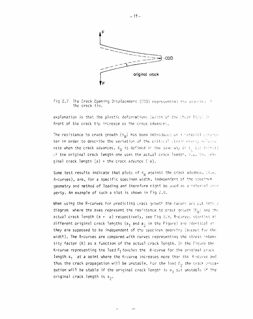
- 1 1 -

original crack

Fig 2.7 The Crack Opening Displacement (COD; representing t'-e w k i c i n : 'the crack tip.

explanation is that the plastic deformations (width of t fie :,h •.•?.»• 1ios" i',

front of the crack tip increase as the crack advances.

The resistance to crack growth (KR) has been introduced cis a ••••aterial : :-.rj-e-

ter in order to describe the variation of the critic il <:. trair. (•'•;>;•:,' '••]•_.•.'•_•

rate when the crack advances. K R is defined in the same way ao \_ t..t \':---\-.\:

o f the original crack length one uses the actual crack length, i.e. the ori-

ginal crack length (a) + the crack advance ( a ) .

Some test results indicate that plots of KR against the crack advance, (i.e.

R-curves), are, for a specific specimen width, independent of the s p e c H e n

geometry and method of loading and therefore might be used as a material pro-

perty. An example of such a plot is shown in Fig 2.8.

When using the R-curves for predicting crack growth the curves are out into a

diagram where the axes represent the resistance to crack grewtn (Kr,) and the

actual crack length (a + :.a) respectively, see Fig 2.9. R-curves starting at

different original crack lengths (a, and a ? in the Figure) are identical as

they are supposed to be independent of the specimen geometry (except for the

width). The R-curves are compared with curves representing the stress inten-

sity factor (K) as a function of the actual crack length. In the Figure the

K-curve representing the load F touches the R-curve for the original crack

length a- at a point where the K-curve increases more than the R -curve and

thus the crack propagation will be unstable. For the load F., the crack propa-

gation will be stable if the original crack length is a. but unstable if the

original crack length is a-.

-12-

K,

Fig 2.8 An example of a crack growth resistance curve (R-curve).

KRorK

(a»Aa)

Fig 2.9 The principles of predicting crack propagation by use of R-curves,

-13-

Kn-curves can be used only if linear elastic fracture mechanics is a"-jlic

for each value of the crack advance but the R-curve analysis of course c i

also be relevant for JR-curves, CODR-curves and so on.

2.4 Fracture mechanical models considering the influence t r i e f r a c

zone

The crack model presented in Fig 2.10a was used by Andersson and 3en,:v

(1970). A layer of thickness d was inserted between two se-i-infinito,

nearly elastic media and by interrupting the layer a crack couli be ":o

The layer was given a stress-deformation relation according to Fi<-: 1.'

The slope of the ascending part of the stress-deformation corje was i_n.

so that it was in agreement with the stress-strain curve for the se-i-

te media. For different assumptions of the slope of the descend inc. :\v

the curve in Fig 2.10b, the stress-distribution in front of the crack

could be calculated by use of numerical methods. However, the '"esults

primarily of theoretical interest due to poor knowledge about tnt- -;at-j

perties necessary to determine the stress-deformation curve in r;- _'

i i -

3 ro

Deformation

b)

F i g 2 . 1 0 a ) T h e c r a c k m o d e l a c c o r d i n g t o A n d e r s s o n a n d B e r g k v i s t ( V J 7 ' ) ) .

b ) S t r e s s - d e f o r m a t i o n r e l a t i o n f o r t h e t h i n l a y co r i n i 'i ' . i '•<•).

- 1 4 —

In damdge mechanics (Kachanov, 1958) the strength

tenm'ned by the deterioration of the material caused by the loading. The value

of the deterioration is characterized by a parameter .j, which is a measure of

the decrease in the load carrying internal area of the material. The net

stress in the undamaged material (s) then equals ••;/{ 1-. ) where •: is the con-

ventional stress applied to the material.

Janson and Hult (1977) combined damage mechanics and the Dugdale model. In the

Dugdale model the stress is constant along the plastic zone in front of the

crack tip. Janson and Hult replaced the constant stress by a constant net

stress (s) and let . be dependent on the distance from the crack tip, which

resulted in a varying stress along the yield zone. The same principles as used

for the Dugdale solution could then be used for calculating the length of the

yield zone as a function of the applied stress for different assumptions of

the distribution of ... All the calculations were carried out on an infinite

plate containing a slit. In another paper (Janson, 1978) calculations were

presented, where ,; increases 1 inearly with the widening, in the stressed direc-

tion, of the fracture zone. The calculation results are in good agreement with

the solution according to Dugdale for small values of the crack length and in

good agreement with the solution according to linear elastic fracture mecha-

nics for large values of the crack length. However, in an intermediate range

the varying stress along the yield zone, or fracture zone, affects the calcu-

lation results considerably.

Naus and Lott (1968) used a crack model similar to that in Fig 2.12 in order

to estimate the length of the fracture zone in front of a crack tip in cement

paste. However, they did not relate the stress in the thin layer to the defor-

mation of the layer but assumed a certain stress distribution along the frac-

ture zone.

By use of damage mechanics and the finite element method Mazars (1981) studied

the development of fracture zones in plain and reinforced concrete specimens.

The method is not a pure fracture mechanical method and so far only initially

unnotched specimens have been analysed.

-15-

3 THE FICTITIOUS CRACK MODEL

3.1 The tensile fracture of concrete

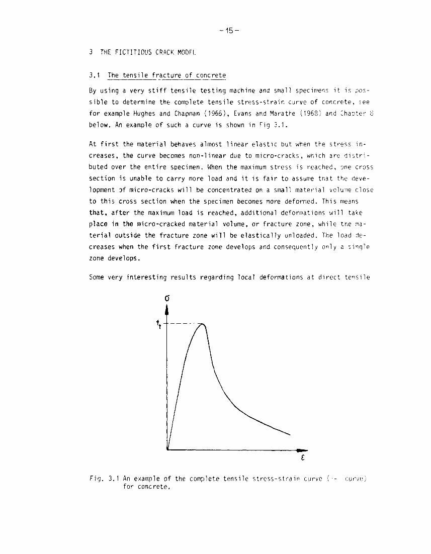
By using a very stiff tensile testing machine and small specimens it is pos-

sible to determine the complete tensile stress-strain curve of concrete, see

for example Hughes and Chapman (1965), Evans and Marathe (1968) and Chapter 8

below. An example of such a curve is shown in Fig 3.1.

At first the material behaves almost linear elastic but when the stress in-

creases, the curve becomes non-linear due to micro-cracks, which are distri-

buted over the entire specimen. When the maximum stress is reached, one cross

section is unable to carry more load and it is fair to assume that the deve-

lopment of micro-cracks will be concentrated on a small material volume close

to this cross section when the specimen becomes more deformed. This means

that, after the maximum load is reached, additional deformations will take

place in the micro-cracked material volume, or fracture zone, while the ma-

terial outside the fracture zone will be elastically unloaded. The load de-

creases when the first fracture zone develops and consequently only a sinqle

zone develops.

Some very interesting results regarding local deformations at direct tensile

Fig. 3.1 An example of the complete tensile stress-strain curve (for concrete.

curve;

-16-

tests were presented by Heilmann, Hilsdorf and Finsterwalder (1969). Results

from one of their tests are presented in Fig 3.2. Strain gauges were glued

at different positions on a 600 mm long concrete specimen with a cross sec-2

tional area of 80 x 150 mm , see Fig 3.2a. The load was excentrically app-

lied, which made it possible to achieve a stable fracture. In the Figure the

position of the final crack is shown.

In Fig 3.2b the local strains are shown as a function of the mean strain of

the specimen. The local strains are separated into two groups; one group re-

presenting the cross section where the final crack develops (gauges 2-3) and

one group representing the material outside the position of the final crack

(gauges 1, 4-9). As can be seen in the Figure, the strain represented by the

gauges crossing the final crack increases rapidly from the moment when the

maximum stress is reached. At the same time the strain outside the fracture

zone decreases. This clearly shows that a local fracture zone starts deve-

loping when the tensile stress is reached. In this case the fracture zone in

fact starts developing already before the maximum stress is reached, but this

is explained by the excentricity of the load, which means that the fracture

zone propagates from one side cf the specimen, through the material, to the

other side. However, the development of the fracture zone mainly takes place

after the maximum stress is reached.

In Fig 3.2c the local strains for the individual gauges are shown for diffe-

rent stress levels. The strains increase very rapidly for the two gauges over

the fracture zone while the strains over the other gauges remain fairly low.

This implies that the fracture zone is located to a narrow band across the

specimen.

As the width of the fracture zone in the stressed direction seems to be small

it ought to be possible to describe the tensile test by a simple model accor-

ding to Fig 3.3.

In the model the fracture zone is replaced by a slit that is able to transfer

stress and the stress transferring capability depends on the width (w) of the

slit. The width of the slit is zero when it starts opening and consequently

the length of the specimen outside the slit (or fracture zone) equals the o-

riginal specimen length (?.)+strain deformations. The total deformation (/u)

of the specimen then becomes:

AP, = cQi + w (3:1)

where G is the strain in the material outside the fracture zone.

- 1 7 -

b)

c)015

010

005.

- O 3, .C3MPO

t 2 3 4 5 6 7 8 9 Gauge

Fig. 3.2 a) The position of the 9 strain gauges.

b) Strains for the gauges crossing the fracture zone (2-3) and forthose outside the zone (1, 4-9). -^strain tor gauge fio i, ,„--=mean strain for the specimen.

c) Strains for the individual gauges for different stresses.(Heilmann, Hilsdorf and Finsterwalder, 1969)

- 1 8 -

i l T TT

clUTIT,

Stress transferring/sl i t

}w

Fig. 3.3 A simple model of the direct tensile test. The fracture zone isreplaced by a slit that is able to transfer stress. The stresstransferring capability depends on the width (w) of the slit.

From (3:1) it is obvious that the mean strain (e ) of the specimen in Fig 3.3

is:

cm = t.Q + w/J. (3:2)

w is zero before the tensile strength is reached and consequently the mean

strain is independent of the specimen length for the increasing part of the

stress-strain curve. However, after the maximum stress is reached, the defor-

mation of the fracture zone affects the mean strain and consequently the

stress-strain curve of concrete, and of other non-yielding materials, is

dependent on the specimen length. This means that it is unsuitable to use the

stress-strain curve as a material property. A better way of describing the

deformation properties of a material therefore is to use two relations; one

relation between the stress and the relative strain for the material outside

the fracture zone (Fig 3.4a) and one relation between the stress and the ab-

solute deformation of the fracture zone (Fig 3.4b)

The fracture zone of a non-yielding material can be compared with the necking

of a yielding material. However, there is one fundamental difference. The

necking is caused by shear deformations and therefore the properties of the

- 1 9 -

a) b)

Fig. 3.4 a) The deformation properties of the material outside the frac-ture zone are given by a relation between the stress and therelative strain, i.e. a o-t curve.

b) The deformation properties of the fracture zone are given bya relation between the stress and the absolute widening of thezone in the stressed direction, i.e. a _-w curve.

necking zone are strongly affected by the state of stress, plane stress or

plane strain, which means that the properties of the necking zone depend on

the specimen thickness. The fracture zone of a non-yielding material is cau-

sed by the development of micro-cracks and no shear deformations take place.

This means that the difference between plane stress and plane strain is small

for concrete and therefore the :.--. and c-w curves ought to be independent of

the specimen thickness and, consequently, the curves in Fig 3.4 can be consi-

dered as material properties.

3.2 The Fictitious Crack Model and its applicability

When a notched specimen of a linear elastic material is subjected to load,

the stress in front of the notch will, at least theoretically, approach in-

finity. This of course is impossible for a real material. In the case of con-

crete, or other non-yielding materials, a zone of micro-cracks will develop

in front of the notch and this fracture zone considerably reduces the stress

-20-

concentration and this results in a much more realistic description of thestress distribution than the linear elastic solution, see Fig 3.5.

The fracture zone in front of a notch normally develops in a tensile stressfield and consequently the properties of this zone are similar to those ofthe fracture zone in a direct tensile test. This means that it ought to bepossible to approximate the fracture zone in front of a notch with a slit, orcrack, that is able to transfer stress, see Fig 3.6. The stress transferringcapability depends on the width of the slit in the stressed direction. In theFigure the load is represented by a point load but of course this descriptionis relevant for all types of loads, including volume stresses due to shrin-kage- or temperature gradients.

The stress transferring crack is not a real crack but can be considered as afictitious crack and therefore the model described above is called the Fic-titious Crack Model. When using the Fictitious Crack Model the following as-sumptions are made:

* The fracture zone starts developing at one point when the firstprincipal stress reaches the tensile strength. Of course othermore complicated fracture criteria can be used but often the simpletensile strength criteria is sufficient.

* The fracture zone develops perpendicular to the first principalstress.

* The material in the fracture zone is partly destroyed but is stillable to transfer stress. The stress transferring capability dependson the local deformation of the fracture zone in the direction ofthe first principal stress. In the calculations the fracture zoneis normally replaced by a stress transferring crack and the stresstransferring capability depends on the width of the crack in thestressed direction according to a a-w curve, see Fig 3.4b.

* The width of the fracture zone in the stressed direction is assumedto equal the widening of the zone, i.e. the width of the zone iszero when it starts developing. For non-yielding materials thisshould be a fair assumption.

* The properties of the material outside the fracture zone are given

in a o-e curve, see Fig 3.4a.

- 2 1 -

• t t t

i

f

bv ~-

ta

Fracture

. /

//

\

i

zone

t

t '

.

t 1i a

Fig 3.5 Probable stress d i s t r i b u t i o n in f r on t of a notch f o r a l i neare las t i c material (a) and fo r a non-y ie ld ing material wi th amicro-cracked zone in f ron t of the notch t i p (b ) .

a) b)Fig 3.6 When using the Fictitious Crack Model, the fracture zone in front

of a crack tip (a) is replaced by a crack that is able to trans-fer stress (b). The stress transferring capability depends on thewidth of the crack according to a <-w curve.

-22-

The fracture zone starts developing in one point when the first principalstress reaches the tensile strength even if the high stress is due to otherreasons than a stress concentration in front of a notch tip. This means thatthe Fictitious Crack Model is not a pure fracture mechanics model but ini-tially unnotched structures can also be analysed. This is one thing thatmakes the Fictitious Crack Model differ from most other approaches. Anotheradvantage is that, by using the Fictitious Crack Model, it is possible tostudy the development of the fracture zone, the initiation of crack growthand the propagation of the crack through the material. When other models areused, normally only the initiation of crack growth is analysed.

The description of the Fictitious Crack Model above is relevant for a homo-geneous material, i.e. a material that has the same properties in all points.In reality no materials are perfectly homogeneous, at least not in the atomicscale. However, if the analysed structure is a few times greater than thelargest irregularities in the material, then the material in the structurecan be assumed to be approximatively homogeneous and the o-w curve is then afunction of the fractions and the properties of the components of the mate-rial .

In this thesis the materials are always assumed to be homogeneous but theFictitious Crack Model can be used for analysing heterogeneous materials aswell. For example, the Barenblatt model is identical to the Fictitious CrackModel when applied on the atomic scale, where, as mentioned above, materialscan never be considered as homogeneous. When studying materials that are he-terogeneous on the macroscale, for example reinforced concrete, it is neces-sary to know the material properties, including the a-w curves, for the dif-ferent components of the material as well as the properties of the contactzones between the components. Some results from such calculations are presen-ted by Modéer (1979) and Petersson and Gustafsson (1980).

- 2 3 -

4 THE FINITE ELEMENT METHOD APPLIED TO THE FICTITIOUS CRACK MODEL

4.1 Introduction

The Dugdale model is a special example of the Fictitious Crack Model whichcan be treated analytically. However, the Fictitious Crack Model normally hasto be treated by using numerical methods and the Finite Element Method (FEM)then seems to be the most suitable method. When using FEM the closing stres-ses actingacross the fracture zone (Fig 4.1a) are replaced by nodal forces(Fig 4.1b). The intensity of these forces of course depends on the width ofthe "fictitious" crack according to the a-w curve of the material. When thetensile strength, or another fracture criterion, is reached in the top node,see Fig 4.1b, this node is "opened" and forces start acting across the crackat this point. In this way it is possible to follow the crack growth throughthe material.

a)

K - - .

! r-

- -I- f-

_ r \t

— t t

• f

3 '

' Topnode

4:i I I :b)

Fig 4.1 When using FEM, the stresses acting across the "fictitious"crack (a) are replaced by nodal forces (b).

4.2 Calculation method I: substucture

In Fig 4.2 a schematic illustration of a deeply cracked structure that issubjected to load is shown. This type of structure is used as a base in thiscalculation method and at the calculations the fracture zone can develop onlyalong the crack, see below. The dots on the boundaries of the crack representfinite element nodes. The position of the two nodes in each node pair (a node

node n

Fig 4.2 A schematic illustration of the finite element nodes along thecrack boundaries in a deeply cracked specimen.

pair is the two nodes en the opposite crack surfaces at the same distancefrom the crack tip) will coincide when the structure is unloaded. The nodepairs are numbered from 1 at the base of the crack to n+1 at the crack tip.The distance between two pairs of nodes i and i+1 is denoted a-.

As the development of the fracture zone is restricted to take place along thecrack it is favourable if the crack is as deep as possible. However, to de-scribe the stresses and strains in a realistic way, a sufficiently number ofnodes must be left between the crack tip and the loading point and for a gi-ven finite element mesh this is the only restriction for the largest possiblevalue of the crack depth.

By introducing closing forces over the crack it is possible to make the struc-ture in Fig 4.2 relevant for an arbitrary notch depth, see Fig 4.3 where anexample of a notch with the tip at node k is illustrated. If the material is1inear elastic and if thp deformations are small, the widening of the crackat each node point from node 1 to node n can be expressed by the n equations:

n ....C(i)F (4:1)

- 2 5 -

undamagedmaterial

node k realcrack

Fig 4.3 A schematic i l l u s t r a t i o n of the f i r s t load step in calculat ionmethod I .

undamagedmaterial

Fig 4.4 A schematic i l lustrat ion of the second load step in ca lcu la t ionmethod I .

-26-

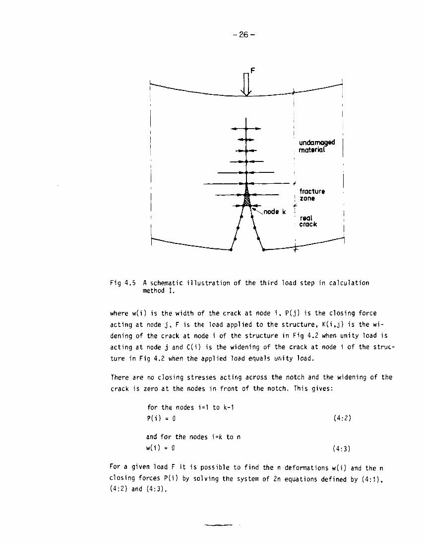
Fig 4.5 A schematic illustration of the third load step in calculationmethod I.

where w(i) is the width of the crack at node i, P(j) is the closing forceacting at node j, F is the load applied to the structure, K(i,j) is the wi-dening of the crack at node i of the structure in Fig 4.2 when unity load isacting at node j and C(i) is the widening of the crack at node i of the struc-ture in Fig 4.2 when the applied load equals unity load.

There are no closing stresses acting across the notch and the widening of the

crack is zero at the nodes in front of the notch. This gives:

for the nodes i=1 to k-1P(i) = 0

and for the nodes i=k to nw(i) = 0

(4:2)

(4:3)

For a given load F it is possible to find the n deformations w(i) and the nclosing forces P(i) by solving the system of 2n equations defined by (4:1),(4:2) and (4:3).

-27-

The displacement (•) of the loadinn point is:

5 = ? D(i)P(i) + D FF .;:-i;i-1

where D(i) is the displacement of the loading point of the strictjre in

Fig 4.2 when unity load acts at node i and D r is the displacement of the

loading point of the structure in Fig 4.2 when the applied load equals

unity load.

All the constants above, K(i,j), C ( i ) , D(i) and Dp, are determined by n e ^ s

of finite element calculations. When determining the constants a nu-i-o-- o f

different load cases are solved but the same global stiffness -latri.. c ^ De-

used for all the load cases and consequently it is only necessary to c^-'-y

out a single invertation of the stiffness matrix.

The solving of the system of equations above, which is the r'nii sten of

this calculation method, results in the initial slope of the load-displace-

ment curve (F-5 curve).

The structure in Fig 4.3 is linear elastic and consequently the stress M

the notch tip will exceed the tensile strength as soon as the structure be-

comes subjected to load (unless the structure is initially unnotched). "here-

fore the second step in this calculation method is to "open" the node cair K

at the notch tip and to introduce a closing force at this point, see riq 4.4.

The intensity of this closing force depends en the widening of the crack

accordingto the J-W curve:

Pfk) = a kb-(w(k})/2 (4:ra.

where a. is the distance between the nodes k and k + 1, b is the width :••:" t ho

structure and ~(w) is the stress transferring capability as ?. function of

the widening of the crack according to the --w curve. As th»? closing stro%-

ses are zero on the "notch" side of the node k, it is only the st-'e • vr-, ac-

ting on the area a.b/2 that affect the force P f k ) .

In order to facilitate the calculations it is suitable to apnroyriate the

j-w curve with straight lines. The simplest approximation is a single, de-

scending, straight line, see Fig 4.6a. In the Figure f. is the tensile

strength and w is the maximum widening of the fracture zone when it is still

able to transfer stress. The area under the curve represents the amount of

energy necessary to create one unit of $rea of a crack and consequently the

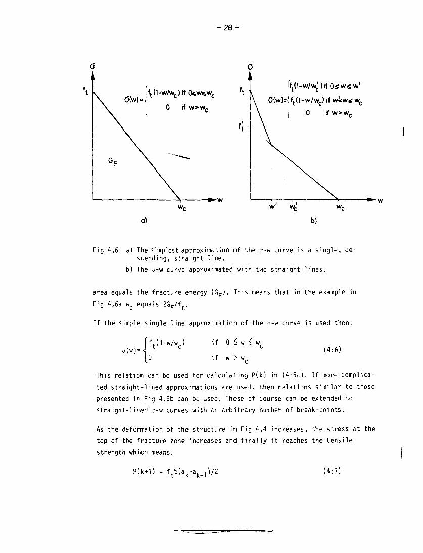
- 2 8 -

w1

a) b)

Fig 4.6 a) The simplest approximation of the a-w curve is a single, de-scending, straight line.

b) The J-W curve approximated with two straight lines.

area equals the fracture energy (Gp). This means that in the example in

Fig 4.6a w equals 2Gp/ft.

If the simple single line approximation of the a-w curve is used then:

if 0 < w 1 w.o(w) =

ft(1-w/wc)

0 if w > w.(4:6)

This relation can be used for calculating P(k) in (4:5a). If more complica-ted straight-lined approximations are used, then relations similar to thosepresented in Fig 4.6b can be used. These of course can be extended tostraight-lined a-w curves with an arbitrary number of break-points.

As the deformation of the structure in Fig 4.4 increases, the stress at the

top of the fracture zone increases and finally it reaches the tensile

strength which means:

(4:7)

-29-

During the first step of the calculation the deformation at node k wtib zeru.

If this condition is replaced by (4:5a), then ( 4 : 1 ) , ( 4 : 2 ) , (4:3) and (4:7)

result in a system of 2n + 1 equations and by solving this system it is pos-

sible to determine the n nodal deformations, the n nodal forces and the load

for the moment when the tip of the fracture zone will advance. After t'"ns one

has to check the widening of the fracture zone at node k. If this exceeds a

critical point of the J-W curve, see Fig 4.6, it is necessary to change

(4:5a) so it fulfils the ;-w relation, and then this new system of equations

has to be solved. This is repeated until the :-w relation is fulfilled.

The displacement at the point of the applied load is calculated by usinq

( 4 : 4 ) , which together with F produces the first point of the load-displace-

ment curve. All the calculations in this second step can be carried out with-

out any finite element calculations as all the constants are the same as fo>"

the first step.

During the third step the node pair k+1 is "opened" and a closing force

starts acting at this point, see Fig 4.5. For this interior node pair, clo-

sing stresses act on both sides of the node and therefore the closing force

becomes:

P(k + 1) = ( a k + a k + 1 ) t H w ( k + 1 ) ) / 2 .4:5b)

The criterion for propagation of the fracture zone is that P(k+2) exceeds

f t b ( a k + 1 + a k + 2 ) / 2 (compare (4:7)). This criterion plus ( 4 : 1 ) , (4:2) and

(4:3) (where the conditions w(k)=0 and w(k+1)=0 are replaced by (4:6a) and

(4:5b) respectively) give the necessary 2n+1 equations. After solvinn this

system of equations the widening of the fracture zone is controlled and even-

tually some adjustments of the system of equations have to be carried .'.*:.

The calculated value of F together with (4:4) give the second liomt of the

"load-displacement curve. Note that no new finite element t.al c i1 at i •jn ••, (Un-

necessary for this third step either.

The development of the fracture zone and the growth of *he real •.-•;>.(.k <.<•.<•

then be followed step by step in the san;e way until the fraeVjrt: /one rt-fv h: ,

node n and the load-displacement curve of the structure is derived.

The node number (k) for the position of the notch tip tan be tho^en between

1 and n and consequently it is possible to change the initial notch depth

without changing the constants in the system of equations. If k 1 then the

structure is initially unnotched.

-30-

The stresses along the crack can, for each step, be calculated as:

• . for i=k (at the notch tip)

(4:8)2P(i) for i >t k

where c(i) is the stress at node i. The stresses and strains in trie elements

outside the crack propagation path can be derived from equations similar to

(4:4).

All the constants K(i,j), C(i), D(i) and Dp are determined on structures si-

milar to the one presented in Fig 4.2. When the material in the structure is

linear elastic, the constants can be converted, by using simple linear elas-

tic relations, to be relevant also for other dimensions and other deforma-

tion properties (Young's modulus). In Table 4:1 the proportionality factors

are given for the different constants. In the Table the proportionality fac-

tor for the distance (a-) between two nodes is also shown.

Table 4:1 Proportionality factors for the constants in (4:2)-(4:8).d=some characteristic dimension of the structure in the plane.b=the width of the structure perpendicular to the plane,E=Young's modulus.

Constant

K(i,j)

C(i)

D(i)

DF

ai

Proportionalityfacto.

1/bE

1/bE

1/bE

1/bE

d

The proportionality factors in Table 4:1 are relevant only if the dimensions

in the plane are uniformly changed. For example, where a beam is concerned

it is necessary for the ratio beam depth/beam length to remain constant. How-

ever, in some cases it is possible to approximately convert the constants to

be relevant for other dimensions even if the dimensions in the plane are non-

uniformly changed. For a notched beam in three-point bending the values of

K(i,j) ought to be independent of the beam length, at least when the ratio

beam length/beam depth is not too small. The opening of the crack depends

only on the moment at the notched cross section. This moment increases li-

-31-

nearly with the beam length and therefore C(i) ought to he proportional * ;

the length. Then according to the Maxwel1-Bettis theorem L U iv is also :<CJ-

portional to the beam length. Dp is the deflection of the lending point v.ncr

the applied load F equals unity load. The value of D r for a linear oKi^ti'.

material can be calculated for an arbitrary bea:" lennth •;•".;. M ss/.r-. i.vY :

wher e b-beam w i d t h , d=beai!) d e p t h , .-beam length, a-notch c'ei'fn ,;". - vo..n:' ••;

d u l u s . The function g.(a/d) is shown in Fig 4.7. In U : ' - the in'-'ljence ~)c

Poisson's ratio is neglected w h i c h , at least where concrete and s i : ; n a r -"J1-

terials are co n c e r n e d , affects the value of D F very l i t t l e .

Cement i tious materials are cften subjected to volume s t r e s s e s due t.> dry in-,

s h r i n k a g e and temperature gradients for e x a m p l e . Most available F[M-progra:;s

can be used for treating this type of loading for linear elastic m a t e r i a l s .

When the structure in Fig 4.2 is subjected to shrinkage stresses "or ex a m p -

l e , the separation of the nodes in each node pair along the crack can be de

g.la/d)

10

0.10.5 1.0

a/d

Fig 4.7 The function g^a/d) used in (4:12)

-32-

termined. By introducing these values in (4:1), the influence of volume

stresses can be analysed by means of the Fictitious Crack Model:

" + C(i)F + w.(i) (4:13)

where Ww(i) represents the separation of the nodes in the node pair i when

the structure is subjected to a certain distribution and intensity of volume

stresses. The values of w,,(i) are derived from linear elastic FEM calcula-

tions and consequently they can easily be converted to being relevant also

for other intensities, specimen dimensions and for other values of the

Young's modulus.

One limitation of the calculation method described above is that it is ne-

cessary to know the crack propagation path in advance. However, this is of-

ten the case due to symmetry of geometry and loads, existence of weak zones,

test results or experience for example. If the crack propagation path is

known in advance, then there are many advantages for using this method. When

the values of the constants K(i,j), C(i), D(i) and Dr are determined once,

the calculations can easily be carried out by solving the system of 2n+1

equations for different notch depths, different specimen dimensions, diffe-

rent values of the Young's modulus and different shapes of the a-w curve.

The influence of volume stresses can also be analysed. The solving of the

2n+1 equations (normally n<40 is sufficient) requires much less computer ca-

pacity than analysing the global stiffness matrix of the structure and con-

sequently the calculation costs are reduced considerably.

4.3 Calculation method II: the su_per_pqs_itu)n principle

Sometimes it is impossible to predict the crack propagation path in advance,

in which case the calculation method I is useless. When using the method of

superposition the first step is to apply the load F1 to the linear elastic

structure in Fig 4.8a, which gi»es the stress .-(1,i) in each node i. The

load F. is chosen so that the tensile strength is reached at the crack tip,

i.e. .7(1,1)=ft.

The second step is to "open" node 1 and to introduce opening forces across

the crack at this node, see Fig 4.8b. The intensity of the forces must de-

pend on the width of the "fictitious" crack according to the <-w curve and

on the area which is represented by the forces. For the simple straight-li-

ned •.;-w curve in Fig 4.6a, the intensity of the forces increases linearly

from 0 to a.bf. 12 when w increase from 0 to w and the forces a^e 0 when

- 3 3 -

Fig 4.8 Schematic illustration of the three first load steps incalculation method II (superposition).

w > w.. b is the width of the structure perpendicular to the plane and a.

is defined in Fig 4.8a. The load F2 is chosen so that -(1,2)+cr(2,2) = ft which

means that, when loadcase 1 and 2 are combined, the tensile strength is

reached at node 2. The total load is then F.+F? and the stresses at the dif-

ferent nodes are given as a(1 ,i )+?(2,i). The stress at node 1 due to load F~

is negative (the forces at this node want to widen the crack) and conse-

quently the total stress at node 1 decreases according to the r-w curve.

The third step, see Fig 4.8c, is to "open" node 2 and to introduce opening

forces across the crack at this point. The intensity of these forces increa-

ses linearly from 0 to (a.+ap)bftII when w increases from 0 to w (if the

>7-w curve is approximated with a single, straight line). The load F-, is cho-

sen so that J(1,3)+c(2,3)+c(3,3)=f. and the calculations are carried out

exactly as for the second step. In this way it is possible to follow the

crack growth through the material.

The simple example above illustrates a crack propagating along a straight

line. However, by using this method it is possible to chose the propagation

direction of the fracture zone after each calculation step. Then the first

principal stress is calculated at the tip of the fracture zone and the pro-

pagation takes place along a path perpendicular to the first principal

stress or, as the possible directions of propagation are limited to the di-

rections of the element sides, along the element side which deviates less

from the theoretical propagation direction.

This calculation method is much more expensive than calculation method I as

it is necessary to invert the global stiffness matrix of the structure for

each calculation step. Also, there are no simple methods of converting the

calculation results for one specific dimension so that they are relevant

for other dimensions. Therefore method I is much more efficient when it can

be used.

4.4 Element wide fracture zones

For the calculation methods described in 4.2 and 4.3 inter element fracture

zones and cracks are used. This means that the crack propagation path is

bound .to follow the sides of the elements. This gives rise to some problems

if the direction of the propagation path is unknown. In Fig 4.9a an example

of a theoretical direction of crack propagation is shown in a finite ele-

ment mesh with square elements. The elements are numbered from (a,1) to

(j,10). Normally the theoretical propagation path does not follow the ele-

-35-

a)

j

i

h

g

t

e

d

c

b

a

!

i

I I 1

\ .

\

.. l . . _- . i- .

- - r • - • r -T -

X Theoretical prop path• i • . . .

1

1 2 3 4 5 6 7 8 9 10

b)

j

h

9

f

e

d

c

b

a

i 1

, ^. 4 . . - . .

ä_ . ?^i)

^ ^

•• • . • • . • • ' v " x N

1 2 3 A 5

1 i

• • t * r *

Theoretical prop, path

5# ' ' ' "

i11 ,N

61

7 8 9 10

Fig 4.9 a) When inter element crack propagation paths are used, the crackis bound to follow the sides of the elements.

b) When element wide fracture zones are used, the stiffness of theelements is changed when the crack passes through.

-36-

ment sides but an approximate crack propagation path according to the Figuremust be used in the calculations. The element mesh in the Figure is coarseand a finer mesh normally gives a better approximation. It is also possibleto use other element shapes, for example, triangular elements sometimes givebetter possibilities to follow the theoretical propagation path more exact-ly. Another, but more complicated, method is to change the element mesh af-ter each load step so that the element sides coincide with the direction ofthe propagation path.

For each load step nodes have to be "opened". This means that the number of

nodes increases as the fracture zone propagates. This affects the stiffness

matrix and complicates the calculations.

The problems discussed above are not unique for the Fictitious Crack Modelbut apply also to linear elastic finite element calculations. Some of theproblems are solved for the linear elastic case if the Blunt Crack Band Mo-del (Bazant and Cedolin, 1979) is used. In this model an element wide crackis used. When a crack passes through an element, the stiffness of the ele-ment is reduced to zero perpendicular to the direction of crack propagationbut the stiffness parallel to the crack is not changed.

If the Blunt Crack Band Model is applied to the Fictitious Crack Model someproblems are bound to arise. First, the a-w curve is related to the abso-lute deformation of the fracture zone which means that the curve will bedependent on the element size if element wide fracture zones are used. Thisis a small problem as long the fracture zone propagates along a straightline parallel to the sides of rectangular elements, see Fig 4.9b. However,when the direction of the propagation path deviates from the direction ofthe element sides, for example when the fracture zone propagates from ele-ment (c,6) to (d,5), then the width of the element perpendicular to the pro-pagation path varies along the path. This gives rise to difficulties whenchoosing the a-w curve. Furthermore, when the fracture zone advances fromelement (c,6) to (d,5), the fracture zone will be tied at the node betweenthe elements and consequently it is necessary to change the Droperties ofat least one more element, in this case element (c,5). The same problem ari-ses for elements (e,5), (e,3) and (g,4).

According to the discussion abcve it seems doubtful if there are any advan-tages in using element wide fracture zones for Fictitious Crack Model calcu-lations. Inter element propagation paths are preferable, it least when thedirection of the crack propagation path is known in advance.

-37-

4.5 Material parameters affecting the choice of the finite e1ement mesn

When representing high stress gradients by means of FEM it is necessary to

use a fine element mesh. For a linear elastic material the stress in front

of the crack tip increases very rapidly as the distance from thr notch tip

decreases and consequently, in order to describe the stress distribution in

a proper way, one has to use a great number of small elements and sometimes

even a special crack tip element. The stress singularity disappears when

there is a fracture zone in front of the crack tip and the stress distribu-

tion around the tip becomes smooth. This means that the stress field around

the crack tip can be properly described by FEM even if a rather coarse ele-

ment mesh is used. When discussing the choice of element size for Fictitious

Crack Model calculations it is therefore necessary to consider the proper-

ties and behaviour of the fracture zone in the discussion.

The properties of the fracture zone are determined by the _--w curve (Fig

3.4b). The behaviour of the fracture zone is also affected by the properties

of the material outside the zone. These properties are determined by the

o-e curve (Fig 3.4a).

In all the calculations presented in this thesis the c-c curve is approxima-

ted with a straight line according to Fig 4.10a, which ought to be reasonable

for most cementitious materials except when they are highly fibre-reinforced.

The straight-lined a-e curve is defined by the Young's modulus (E) and the

tensile strength (f t).

In the calculations stepwise linear o-w curves are used, see Fig 4.10b. The

area under the curve corresponds to the amount of energy that is necessary

to create one unit of area of a crack and consequently the area equals the

fracture energy (Gp). This means that when the shape of the curve is known,

the position of the a-w curve is defined by the fracture energy and the ten-

sile strength. The shape of the curve is defined by a function h(w/wc) and

the a-w curve can be expressed as:

o(w) = fth(w/wc) (4:14)

The notations in the equation are given in Fig 4.10. h(w/wc)=l when w=0 and

h(w/wc)=0 when w=wc.

The brittleness of a material is characterized by the c-t and the a-w curves.

However, sometimes it is possible to replace these curves with a single, cha-

-38-

a)

Fig 4.10 a) The a-e curve approximated with a single, straight line.b) Normally stepwise linear o-w curves are used in the cal-

culations.

racteristic parameter. When a crack propagates, energy is consumed by thefracture zone. At the same time elastic energy is released from the materialoutside the fracture zone. When the maximum load in a direct tensile test isreached, the elastic energy available for crack propagation is F 5/2=F*:/2k,where F is the maximum load, 6 is the corresponding deformation and k isthe stiffness of the specimen. For a specimen with constant cross section k==AE/ii where A is the cross sectional area and s. is the specimen length. Thismeans that the energy available for crack propagation is F z/2AE. The amountof energy that can be consumed by crack propagation is GpA. By equating the-se two expressions for energy, we find that z* - 2GrA E/Fc = 2GpE/f£, where£*is the length of the specimen when the energy available for crack propaga-tion, at maximum load, equals the capability of energy consumption of thefracture zone. For a given shape of the a-w curve the material then becomesmore sensitive to crack propagation, and therefore more brittle, when thevalue of z*decreases. For practical reasons it is more suitable to use halfthis length to characterize a material and then the characteristic length(i . ) is defined as:

• ¥ '(4:15)

-39-

It must be observed that i. . should only be used for comparing materials

with similar shapes of their o-w curves. However, for materials with similar

shapes of their o-w curves, i . is probably the best way of characterizing

the brittleness; the shorter *. . is, the more brittle the material is.

In this work the well-known three-point bend test on notched and unnotched

beams is analysed and the calculation method I (substructure) is normally

used. For most of the calculations the necessary constants (K(i,j), C(i),

D(i), Dp) were determined by use of the finite element mesh shown in Fig

4.11. As the three-point bend test is symmetrical it was only necessary to

use half the beam in the calculations. The line of symmetry in the Figure de-

fines the middle of the beam. The length/depth ratio of the beam is 4.

The finite elements are four node isoparametric membrane elements and trian-

gular constant strain membrane elements respectively. For the FEM-calcula-

tions the program EUFEMI was used, which was developed at the Division of

Solid Mechanics at the Lund Institute of Technology (Kernelind and Pärle-

tun, 1974).

In order to study how well the behaviour of the material is described when

the element mesh in Fig 4.11 is used and to see how the calculation results

are affected when varying distances between the closing forces in the fractu-

re zone are used, the load-deflection curves for three different beams were

determined. The depths (d) of the beams were 0.2, 0.8 and 1.6 m respectively.

For all the beams the ratio notch depth/beam depth (a/d) was 0.4 and the beam

width (b) was 1 m. The o-w curve was approximated by a single, straight line

and the values of Gp, E and ffc were 100 N/m, 40,000 MPa and 4 MPa respective-

ly, which gives a c .-value of 250 mm. These material properties represent a

normal concrete quality (see Chapter 7 ) .

The calculation results are presented in Fig 4.12. The unbroken curves repre-

sent calculations where closing forces act at each node in the fracture zone

which means that the distances between the forces are d/40. The dashed curves

represent calculations where closing forces act at each second node in the

fracture zone and the distances between the closing forces art then 6/20. In

che Figure the initial slope according to the linear elastic solution i'-. al-

so shown. This slope was calculated by use of (4:12).

The agreement between the initial slope of the curves and the slope -K.cor-

ding to the linear elastic solution seems excellent. This implies that t'in-

finite element mesh used is sufficiently fine for describing \.\v> behaviour

Y

1/1

O).c

C

T )

13O)

OJ

4 -

20

Closing forcas at:tach nodeeach second node

a/cUCUb=1mGp=lOO N/mE =40.000 MPQ

200 300 400 6 (wm)

F i g 4 . 1 2 C a l c u l a t e d l o a d - d e f l e c t i o n c u r v e s f o r d i f f e r e n t b e a m d e p t h s a n j d i f f e r e n t d i s t a n c e s b e t w e e n t h e c l o s i n g f u rc e s in t h e f r a c t u r e z o n e . T h e s t r a i g h t l i n e r e p r e s e n t s t h e l i n e a r e l a s t i c s o l u t i o n d e c o r d i n e j t o ( 4 : l i ? ) .

-42-

of the material outside the fracture zone.

There are differences between the curves representing different distances be-

tween the closing forces. The differences increase as the beam depth increa-

ses but the agreement also seems suprisingly good for the largest beam. This

implies that the properties of the fracture zone can be described in a reaso-

nable way even when the distances between the closing forces are wide. For

the largest beam the distances between the closing forces are 40 and 80 mv\

respectively which correspond to about 15 to 30 . of the characteristic

length. However, these figures are naturally also dependent on the absolute

dimensions of the structure. For example, for small structures (d/ . <1) it

is necessary to decrease the distances between the closing forces.

Other calculation results presented by Petersson and Gustafsson (1980) sup-

port the results above which prove that the Fictitious Crack Model describes

the crack propagation in a proper way, even if the finite element mesh is re-

latively coarse and the distances between the closing forces are wide. How-

ever, it seems unsuitable to use larger distances between the closing forces

than 0.2 >. , , which for concrete corresponds to 40-80 mm.

- 4 3 -

5 THE FRACTURE ZONE

5.1 The width of the fracture zone

The strain measurements presented in Fig 3.2 indicate that the fracture zone

in concrete propagates along a narrow band and that the width of the zone is

small in the stressed direction. Direct observations of stable crack prooa-

gation in fine-grained mortar (maximum aggregate particle size = 0.3 mm) was

reported by Mindess and Diamond (1980). They used a scanning electrone micro-

scope (SEM) in order to study the region in front of a notch in compact ten-

sion specimens. Their results show that branch cracks exist and sometimes

also two or more parallel cracks develop simultaneously but the width of the

cracked zone is very limited, in this case less than a few tenths of a mil-

limeter, i.e. similar to the size of the maximum aggregate particles.

Modéer (1979) used an indirect method in order to study the development of

the fracture zone in front of a notch in a bent mortar beam. The surface of

the beam was covered with a water film. When the widening of the fracture

zone reached a certain value the micro-cracks absorbed water from the sur-

face. This reduced the reflexions from the surface which could be reqistra-

ted by use of a camera. According to these tests it seems that the width of

the fracture zone is limited to a band less than a few millimeter wide.

In order to study the development of the fracture zone, stable tensile tests

were carried out. The tests were performed in the very stiff tensile testing

machine presented in Chapter 8. The material used was concrete with a maximum

aggregate particle size of 8 mm and the water-cement-ratio was 0.6. The spe-

cimens were cast in steel moulds and stored in lime saturated water ( + .''0°C)

until one day before testing. During the last day before testing the speci-

mens were insulated with plastic foil. The tests were performed 7 days afte>-

casting. The specimens were kept in the air for a few minutes while they

were fixed into the testing machine which means that the surfaces nc-came

slightly dry. During the tests water was sprayed on all the surfaces but o-e.

When the fracture zone developed, water was absorbed by the ;ofe due to ca-

pillary forces and the zone could b? observed as a dark area on the "dry"

surface.

The results from two tests are presented here. The mean stress-deformation

curve for the two tests is shown in Fiq 5.1. The "dry" surface was pho'onra-

phed in the 9 positions defined on the curve in the Firjure.

-44-

Ö(MPa)

3

123456789

w((urn)

05

1530506580

110170

50

Fig 5.1 The mean stress-deformation curve for the two tests presented inFig:s 5.2-5.3. The figures on the curve correspond to the posi-tions for the photos in Fig:s 5.2-5.3. w = widening of the frac-ture zone.

The results from one of the tests are presented in Fig 5.2. The surface is

cast against a steel mould which means that the surface is covered with a

thin layer of cement paste and therefore no aggregate particles can be seen.

The first sign of a fracture zone can be observed in photo No 3 where small,

dark lines have developed on both sides of the specimen. This photo is taken

when the widening of the fracture zone is about 15 um and the stress has de-

creased to about 60 »' of the tensile strength. The fracture zone ought to

start developing already when the tensile strength is reached but the micro-

cracks are too narrow to be able to transport water until the position of

the load-deformation curve corresponding to photo No 3 is reached. In photo

No 4 the wet band has spread through the specimen. In photo No 5 there is a

small jump in the wet band and at this position a narrow crack can be distin-

guished and in photo No 6 the crack can be seen very clearly. This means

-45-

• • . • * ".••••-..•>•.'•

. • •' ' m » ' • ' •-

, • . * • • " • : - . • • ' • •

. • ' • • »

10 mm

7 '. 8

Fig 5.2 The development of the fracture zone during a direct tensile test.The surface is cast against a steel mould. The photos correspondto the positions on the load-deformation curve in Fiq 5.1.

46-

y

*5

fO.mm

Fig 5.3 The development of the fracture zone during a direct tensile test.The surface is sawn. The photos correspond to the positions on theload-deformation curve in Fig 5.1.

- 4 7 -

that the crack becomes visible when the widening of the fracture zone is

about 25-50 urn. It can be observed that the material is still able to trans-

fer 25 % of the maximum stress when a visible crack has developed across the

specimen. In photo No 9 the widening of the fracture zone is 170 urn but the

material is still able to transfer some percentage of the maximum stress. In

this photo a branch crack has developed on the left side of the specimen.

This branch crack is probably caused by the extraction of an aggregate par-

ticle from the cement paste inside the specimen.

The results in Fig 5.2, and also the other test results discussed above, in-

dicate that the width of the fracture zone is smäll in the stressed direc-

tion. However, these observations are made on surfaces which are cast against

steel moulds and therefore the results are not representative for the mate-

rial inside the specimen. For this reason a specimen was divided by using a

saw and then tested in the stiff testing machine. The results for the sawn

surface are presented in Fig 5.3. Unfortunately the surface was already part-

ly wetted at the start of the test and the dark areas in photo No 1 have no-

thing to do with the fracture zone.

The fracture zone is first seen in photo No 3 when the widening of the zone

is about 15 urn. In photo No 4 it can be seen how the fracture zone starts de-

veloping around an aggregate particle and in photo No 5 the zone has deve-

loped almost completely around the aggregate particle. This means that the

fracture zone is considerably wider in this case compared with the case in

Fig 5.2. The width of the fracture zone seems to be of the same magnitude as

the size of the maximum aggregate particles, i.e. about 8 mm in this case.

This is quite natural as the aggregate particles have to be extracted from

the cement paste before the final collapse of the specimen. However, normal-

ly a width of the fracture zone corresponding to the maximum aggregate par-

ticle size can be considered as small and therefore the Fictitious Crack Mo-

del should be usable for describing the development of the zone.

5 • IJ!e_.4?yiL'opment of the_fracture_ zone

The development of the fracture zone can be analysed by use of the Ficti-

tious Crack Model. In Fig 5.4 the fracture zone and the stress distribution

in front of a notch tip in a beam subjected to three-point bending are shown

for different positions on the load-deflection curve. The beam depth is

0.2 m, the notch depth 50 mm and the beam length 0.8 m. In the calculations

the ,T-W curve is approximated with a single, descending, straight line and

• 4 8 -

F/b(MN/m)

.06

.04

.02

.00

0.8

ft=3MPa

E =30,000 MPal c h = 0.25 m

50 100 150 Deflection 1/um)

Fig 5.4 The fracture zone and the stress distribution in front of thenotch tip for different positions of the load-deflection curve.The Figure is relevant for a 0.2 m deep notched beam (a/d=0.25)in three-point bending and the material properties correspondto a normal concrete quality.

- 4 9 -

f t, E and Gp are 3 MPa, 30,000 MPa and 75 N/m respectively, i.e. .ch = 0.25 m,

which corresponds to a normal concrete quality. The •-•• curve is approximated

with a straight line.

In this Chapter all the diagrams are relevant for .cn = 0.25 m. They can how-

ever easily be converted to be relevant also for other values of .c^ by use

of the proportionality factor d/;cn.

The fracture zone starts developing as soon as the specimen in Fig 5.4 be-

comes subjected to load. In the first position of the load-deflection curve

in the Figure, a small fracture zone has developed. No stresses exceed the

tensile strength. This gives a much more realistic description of the stress

distribution than the linear elastic solution which always, at least theore-

tically, includes a stress singularity. When the maximum load is reached, the

depth of the fracture zone is about 50 mm and the stress distribution is qui-

te different compared with the linear elastic one. These calculations are re-

levant for a 200 mm deep beam. For smaller beam depths, 50 mm is not unusual

in tests, the influence of the fracture zone will be even more pronounced

and it seems quite obvious that it is necessary to consider the effect the

fracture zone has on the fracture process. It can be observed that the mate-

rial at the notch tip is able to transfer stress even when the maximum load

is reached and a real crack, i.e. a crack with stress-free surfaces, will not

propagate until position 3 of the load-deflection curve is reached. This is

very interesting as it clearly indicates that it is necessary to separate the

criterion for the fracture load, which is normally the most interesting, from

the criterion for crack propagation. Finally, at position 4 a real crack has

advanced a distance of about 30 mm.

In Fig 5.5 the load is shown as a function of the position of the tip öf the

fracture zone (defined as the distance from the notch tip) for different re-

lative notch depths. The curves are relevant for 0.2 m deep, normal quality

concrete beams in three-point bending. For the curve representing the unnot-

ched beam (a/d=0) the fracture zone will not propagate until the tensile

strength is reached at the bottom of the beam but for the notched beams the

fracture zone, due to the stress concentrations, starts developing as soon as

the specimen becomes loaded. The circles on the curves correspond to the po-

sitions where a real crack starts propagating and consequently, before thp>e

points are reached, the curves show the depth of the fracture zone. The jepth

of the fracture zone decreases as the notch depth increases which is explai-

- 5 0 -

Load/unit width (MN/m .1O"2)

td = 0.2m

ft =3MPa

E =30,000 MPal c h = 0 .25m

100 150

Position of the tip of the f r. zone

Fig 5.5 The load as a function of the position of the tip of the fracturezone (defined as the distance from the notch tip) for different re-lative notch depths. The curves are relevant for 0.2 m deep beamsin three-point bending. The dimensions and the material propertiesare the same as those used in Fig 5.4. The dots represent the posi-tions where real cracks start propagating.

ned by the simple fact that the available space for the fracture zone decrea-

ses as the notch depth increases.

In Fig 5.6 the depth of the fracture zone at the maximum load is shown as

functions of the beam depth for a normal concrete quality. Also here the

available space plays an important role and the depth of the fracture zone in-

creases with increasing beam depth. However, the increase in the depth of the

fracture zone is less than proportional to the increase in the beam depth and

consequently the ratio depth of the fracture zone/beam depth decreases with

-51-

Depthof fr. zone! mm)

t150

100

50

25

0.0125 0.025 0.05 0.125 0.25 0.5 1.25 25d(m)

Fig 5.6 The depth of the fracture zone at the maximum load as function ofbeam depth for different relative notch depths. The curves are re-levant for three-point bending and the material properties are thesame as those used in Fig 5.4.

increasing beam depth. This means that the fracture behaviour of concrete and

similar materials is size dependent which is illustrated by a number of examp-

les in Chapter 6. For deep beams the depth of the fracture zone seems to reach

a limiting value of about 125-150 mm. The limiting value ought to be dependent

on the test technique, for example where the direct tensile test is concerned

such a limiting value does not exist. Test results presented by Entov and Ya-

gust (1975) indicate that high, local strains exist 50-100 mm in front of the

notch tip in large, centrally notched tensile specimens and results presented

by Sok, Baron and Francois (1979) show high strains several hundreds of milli-

meter in front of the notch tip in large double cantilever beams (the results

according to Sok et al are probably a bit overestimated which is discussed in

6.5). These results confirm the calculation results showing that deep frac-

ture zones develop in front of notches in concrete structures.

-52-

01-)-3 •3 aw

d=0.2m

k ,.

1 1 1 - ^ .

Fig 5.7 The fracture zone and the stress distribution in front of the notchtip at the maximum load for different beam depths. The Figure isrelevant for three-point bending (a/d=0.25) and the material proper-ties are the same as those used in Fig 5.4 (f.=3MPa, GF=75N/m,E=30,000MPa, nch=0.25 m ) . it

53-

It is not only the depth of the fracture zone that is affected by the beam

depth but also the stress distribution within the zone. In Fig 5.7 the stress

distribution at the maximum load in front of the notch tip is shown for diffe-

rent beam depths. The relative notch depth is 0.25 and the results are rele-

vant for a normal concrete quality. The stress transferring capability at

the notch tip decreases as the beam depth increases and consequently a real

crack starts propagating closer to the maximum load for deeper beams. The

fracture zone is more efficient in reducing the stress concentrations at the

crack tip for low values of the beam depth and the stress distribution becomes

more similar to the distribution according to the linear elastic solution as

the beam depth increases. This of course contributes to the size dependency

of the fracture behaviour where concrete and similar materials are concerned.

- 5 5 -

6 THE FICTITIOUS CRACK MODEL vs OTHER APPROACHES

6.1 Introduction

Linear elastic fracture mechanics is the most frequently used approach fo>~ '..e-

mentitious materials but the J-integral, the COD-approach and R-c;.rvos vv/e al-

so been applied to plain and fibre-reinforced concrete. All these sivro^.'-'-s

have, more or less successfully, been applied to metals and mo v t >:-f -^e v;o r--

carried out in the field of fracture mechanics and concrete has t vrx-f"•>"'_• ::e-r

concentrated on experimental tests, where the relevance for concrete -f : h e

existing approaches has been studied. This has resulted in nj-erecir. and • f"e-

contradictory test data concerning K , G , J , COD and R-curves fcr exa-: It-.

In this Chapter these test data are compared with results derived by :<se c +

the Fictitious Crack Model and the usefulness of the approaches when ä - v 1 - ^

to cementitious materials is also discussed.

Four different "model" materials have been analysed. The - curve is 3p;:r:>i-

mated with a straight line for all the materials but the --w curves dre ; .it-

different and are presented in Fig:s 6.1-6.4.

If the shape of the o-w curve is unknown then the straight line approximation

;'SL) according to Fig 6.1 is probably the most rational. For plain concrete

this simple approximation often gives satisfying results, which is discussed

later. Normal values of Gp and f. for concrete are 100 N/m ana 4 ['Pa respecti-

vely, see Chapter 7, and this means that w , i.e. the maximum widening of the

fracture zone when it is still able to transfer stress, in this case is 0.0b m\.

The approximation according to Dugdale (D) in Fig 6.2 is probably most suitable

for yielding materials such as mild steels and many qualities of plastics.

The curve is used here as it is often referred to in the literature. In some

special cases the curve can be used as a rough approximation for some qualities

of fibre-reinforced concretes.

In Chapter 8 results showing the real shape of the --w curve for a number of

concrete qualities are presented. According to these results, the curve in

Fig 6.3 (C) seems to be the best two line approximation for most normal con-

crete qualities. This curve therefore describes the properties of the fracture

zone in concrete in a more realistic and consequently a better way than the

simple approximation in Fig 6.1.

The shape of the c-w curve for fibre-reinforced materials is greatly dependent

- 5 6 -

fi -STRAIGHT LINE (SL)

w

Fig 6.1 The o-w curve approximated to a single, straight line (SL),

DUGDALE (D)

w

Fig 6.2 A o-w curve according to Dugdale (D),

- 5 ? -

u

4-ft

9Wc

CONCRETE (C)

w

Fig 6.3 A two- l ine approximation of the o-w curve that seems to be sui tablefor most normal concrete qua l i t i es (C).

|FRC

0.015 vxfc w

Fig 6.4 An example of a a-w curve representing a fibre-reinforced material(FRC).

-58-

on the type of fibre and fibre content for example. The curve in Fig 6.4shows an example of such a curve. If f. is 4 MPa and Gp- about 1400 N/m, thenthe initial slope of the curve is similar to that of concrete and w is about1 mm. Then this curve ought to represent a fibre-reinforced concrete (FRC)with a fairU low percentage of short fibres.

The calculations in this Chapter mainly deal with the three-point bend test.In the calculations the finite element mesh in Fig 4.11 was used. In Fig 6.5typical load-deflection curves for the four model materials are shown. The cur-ves represent beams that are C.2 m deep, 0.2 m wide, 0.8 m long and the rela-tive notch depth is 0.4. For all the materials the Young's modulus and thetensile strength are 40,000 MPa and 4 MPa respectively. For the c-w curveaccording to Fig 6.4 Gn is 1430 N/m, which, as mentioned above, correspondsto a fibre-reinforced concrete with a fairly low percentage of short fibres.

FIMN-10"2)

(FRC)

d

.2

b

.2

1

.8

a

L

E

AO

t F

100

^30

too 200

Fig 6.5 Calculated load-deflection curves fo- the four model materials pre-sented in Figrs 6.1-6.4. The curves are relevant for three-pointbend tests on notched beams. The dimensions are m for d, b and e,MPa for E and f and N/m for r.

-59-

For the other o-w curves Gr- is 100 N/m, which corresponds to a normal value

for concrete. As can be seen, the shape of the o-w curve considerably affects

the calculation result. This means that the shape of the o-w curve is an im-

portant parameter that has to be considered when analysing the fracture pro-

cess of a material.

6.2 Linear elastic fracture mechanics

6.2.1 Notch sensitivity

In the literature results from a large number of linear elastic fracture mecha-nics tests on cementitious materials are reported, which are discussed in6.2.2. The results from different tests are often conflicting and this hasgiven rise to doubts about the usefulness of fracture mechanics, where concreteand mortar are concerned. Therefore, in order to study the applicability of frac-ture mechanics to cementitious materials, notch sensitivity tests have been

netcarried out. The notch sensitivity is defined as ff /ff (net. flexural ten-

sile strength/flexural tensile strength) where ff for a three-point bendtest on a notched beam is:

ff 75 ? Fc (6:1)f db (dar

where z = beam length, b = beam width, d = beam depth, a = notch depth andnetF = fracture load. ff equals fr when a = 0.

The notch sensitivity for linear elastic materials has been dealt with byZiegeldorf et al (1980). They showed that the notch sensitivity can be ex-pressed as:

fj e t K Tf = x 4 (6:2a)

V Tf ^ ( l ^

where f(a/d) for a three-point bend test is (Brown and Srawley, 1967):

f(a/d) = l.93-3.07(a/d)+14.53(a/d)2-25.ll(a/d)3+25.8(a/d)4 (6:3)

(6:2a) can be expressed as:

y •"" X —rprf Kc

- 6 0 -

By using (6:2b), the notch sensitivity as a function of the relative notch

depth can be described by a single curve according to Fig 6.6.

:.t "•

3.0

2.0

1.0

0.5

Fig 6.6 Notch sensitivity as a function of relative notch depth (a/d) andfr^cT/Kc for materials that can be treated by means of linear elas-tic fracture mechanics.

The curve in Fig 6.6 shows that the beam is most notch sensitive when the rela-

tive notch depth is 0.2-0.3. The notch sensitivity increases with increasing

beam depth and decreasing values of the parameter K /f.. However, the cur^/e

is relevant only when linear elastic fracture mechanics is applicable, which

considerably limits its usefulness. For example, when f f \/d/K is less than 2,

then the notch sensitivity exceeds 1 for all notch depths, which seems unrea-

listic. Furthermore, the notch sensitivity ought to reach 1 when the notch

depth is zero but this is not the case which is explained by the fact that

linear elastic fracture mechanics i? normally not applicable when the relativt.

- 6 1 -

More realistic notch sensitivity curves can be determined by using the Fic-titious Crack Model, see the unbroken lines in Fig 6.7. In the calculationsthe o-w curve was approximated with a single straight line.

lg-W:SLl

0.5 1.0o/d

Fig 6.7 Notch sensitivity as function of relative notch deoth and d/.cncalculated by means of the Fictitious Crack Model (unbroken lines)and linear elastic fracture mechanics (dashed lines) respectively.In the calculations a c-w curve according to Fig 6.1 (SL) was used.

As can be seen in Fig 6.7, notch sensitivity is not a pure material propertyas it is dependent on the specimen dimensions. A normal value of • , for con-crete is 250 mm and consequently a 100 mm deep beam is relatively notch insen-sitive while a 1 m deep beam is considerably affected by a notch. A probablevalue of i , for cement paste is 5-10 mm (Modéer, 1979) which means thatthis material is notch sensitive already at beam depths of 10-20 mm. The re-sults in Fig 6.7 also imply that for notched beams with d/. .-values less

netthan about 1 the approximative fracture criterion f, =fr is usable. However,

-62-

when using this simple criterion it must be remembered that ff depends onspecimen dimensions and fracture mechanical properties of the material, see7.2.

The finite element mesh used in the calculations is too coarse to be used ford/i.-values exceeding about 8 when the distances between the forces in thefracture zone are 0.2£ . . However, when d/s, . increases, the material becomesmore "brittle" and the usefulness of linear elastic fracture mechanics increa-ses. In 6.2.2 and 7.2 the critical strain energy release rate (G ) and the ten-sile strength (f. ) are discussed and it is shown that when linear elasticfracture mechanics is applicable, G = Gr and ft =f r. According to (2:8) and

•net

2 r

1 -

\

\

^ F i c t .

\ ^ Lin. elastic

Cr. Model N ^

• \ .

i i

|a/d = 0.2

i i i

3216

Fig 6.8 The notch sensitivity for the relative notch depth 0.2 as functionsof d/ncn. The curves represent solutions according to the linearelastic fracture mechanics and the Fictitious Crack Model respec-tively.

-63-

(4:15) it is then obvious that Kc/ff = This rTieans tnat the

linear elastic notch sensitivity curve in Fig 6.6 can be related to ... In

Fig 6.8 the notch sensitivity for the relative notch depth 0.2 is shown as

functions of d/s. .. The two curves represent solutions according to linear

elastic fracture mechanics and the Fictitious Crack Model respectively. The

curves are quite different where small values of d/~. , are concerned but the

difference decreases as d/i . increases. For practical applications therefore

the linear elastic solution ought to be usable as an approximation for d/• ,-

values exceeding about 10-20 when the difference between the curves is less

than about 15 •;-.

(J-w.(C)

0.5 1.0a/d

Fig 6.9 Notch sensitivity as function of relative notch depth and d / c ^ cal-culated by means of the Fictitious Crack Model. In the calculationsa two line approximation of the c-w curve (C) according to Fig 6.3was used.

In Fig 6.7 linear elastic notch sensitivity curves for d/• ,-values exceed-

ing 25 are presented (dashed lines). These plus the curves determined by

means of the Fictitious Crack Model give a complete set of notch sensitivity

curves ranging from d/f h=0.1 to d/. u=100-

The notch sensitivity curves in Fig 6.9 represent materials wich a two line

approximation of the J-W curve according to Fig 6.3. The differences between

these curves and those presented in Fig 6.7 are small but the two line appro*'

mation of the J-W curves seems to give a somewhat higher notch sensitivity.

However, for practical applications the curves in Fig 6.7 ought to be suffi-

cient for concrete. For fibre-reinforced materials the _--w curves are often

quite different and then notch sensitivity curves have to be calculated for

each individual material.

.net

o Cement paste? Mortar• Concrete

Beam depth: 50 mm

0.5

Fig 6.10 Experimental determined notch sensitivity curves for cement paste,mortar and concrete (Shah and McGarry, 1971)

-65-

In Fig 6.10 test results for concrete, mortar and cement paste are shown

(Shah and McGarry, 1971). The results are derived from three-point bend tests

on 50 mm deep beams. A normal value of t . for concrete is 250 mm and for mor-

tar 150 mm (see Chapter 7) which corresponds to d/e .-values of 0.2 and 0.33

respectively. The test results show that concrete and mortar are, more or

less, notch insensitive where the actual specimen size is concerned which

agrees well with the theoretical curves in Fig 6.7. The results for mortar

also show a minimum on the curve for a/d=0.2-0.3, exactly the same as for the

theoretical curves.

The only available value of v. , for cement paste is 7 mm for a 7 days old

paste (Modéer, 1979). In Chapter 7 it is shown that the • .-value for con-

crete decreases rapidly with increasing age due to the fact that the tensile

strength increases relatively faster than the fracture energy and the Young's

modulus. The same ought to be relevant for cement paste and a d/. .-value of

10-20 seems realistic in this case.

The test resu'ts indicate that cement paste is highly notch sensitive where

the actual specimen size is concerned and the notch sensitivity is most pro-

nounced when the relative notch depth is 0.25-0.30. This agrees well with the

theoretical curves. However, the tests indicate a somewhat higher notch sen-

sitivity than the calculations which is probably due to the lack of knowledge

regarding the a-w curve and the ».-value of the actual cement paste and per-

haps also to the testing conditions where for example shrinkage stresses can

affect the results.

In Fig 6.11 other test results are presented (Gj0rv, Sfbrensen and Arnesen,

1977), which are also carried out on three-point bent, 50 mm deep beams. In

this case the agreement between the experimental and the theoretical curves

for cement paste is good but the experimental curves indicate that both con-

crete and mortar are notch sensitive. This can be explained by the fact that

the materials used were unconventional; the content of cement paste was about

52 % by volume in the concrete and 68 . by volume in the mortar! This defini-

Ltly means that the J,-values were much lower than those for ordinary con-

crete qualities.

The i .-values for the materials used in the test ought to increase as the

percentage of aggregate increases. Consequently the test results illustrate,

in an excellent way, how the notch sensitivity increases with increasing

d/? L-values, exactly as for the theoretical curves. The entire amount of

-66--

,net

o Cement paste* "Mortar"• "Concrete"• "Lightweight concrete'

Beam depth: 50 mm

0.5 1.0a/d

Fig 6.11 Experimental determined notch sensitivity curves for cementpaste, "mortar", "concrete" and "light-weight concrete"(Gjtfrv, S0rensen and Arnesen,1977)

aggregate in the light-weight concrete was expanded clay. The capability of

this type of aggregate in preventing crack propagation is poor (see Chapter 7)

and therefore the light-weight concrete ought to be almost as brittle as the

cement paste which explains the position of the notch sensitivity curve for

this material.

Experimental results in agreement with those in Fig 6.10 and Fig 6.11 are also

reported by Higgins and Bailey (1976), Hillemeier and Hilsdorf (1977) and Zie-

geldorf, Muller and Hilsdorf (1980).

-67-

6.2.2 K - and G -approaches

The critical strain energy release rate (G ) represents the energy consumption

per unit crack area at the crack tip when the crack propagates, i.e. the amount

of energy necessary to create one unit of area of a crack. However, G is

strictly defined only for linear elastic materials and where other materials

are concerned, G is always an approximate value of the amount of energy ne-

cessary to create one unit of area of a crack.

The fracture energy (Gp) is another measure of the amount of energy necessary

to create one unit of area of a crack. Gp equals the area under the c-w curve

and consequently Gp is not only defined for linear elastic materials but in

principle for all materials in which cracks can propagate.

According to the definitions above it is obvious that G equals GF where li-

near elastic materials are concerned. For this reason the ratio G /Gp ought to

be useful as a measure of how well linear elastic fracture mechanics describes

the fracture of a structure; the closer G /Gp is unity, the better the linear

elastic fracture mechanics approximation is.

In Fig 6.12 the ratio G /Gp is shown as function of d/. , and relative notch

depth for a three-point bend test. The calculations are carried out by means

of the Fictitious Crack Model. In the calculations K was first calculated

according to (2:9) and (6:3) and then these results were converted to G by

using (2:8). The o-w curve was approximated to a single straight line (SL).

As can be seen in the Figure, the ratio G /Gp increases with increasing values

of 6/i . and finally it ought to approach unity. This means:

lim G = Gr- (6:3)d / , c h ^

and consequently, according to (2:8):

lim K = X/GT? (6:4)A / f *•* • r

dAch->,,(6:3), (6:4) and (2:8) show that K /\/O= \/G /Gp and consequently the two ra

tios can be represented by the same curve in log-diagrams where the modulus

of the logscale for K /^GrE* is twice the modulus of the log-scale for Gr/GF

In Fig 6.12 the ratio K /^GpE is represented by the vertical log-scale to

the right.

- 6 8 -

0.1 -

0D50.05

- 0.3

Fig 6.12 Theoretical values of Gc/Gp and Kc/\/GpE' as functions of d/£cn fordifferent relative notch depths. The curves are relevant for three-point bend tests and the c-w curve is approximated with a single,straight line (SL) according to Fig 6.1.

Normally the fracture load is the most interesting thing to study when analy-sing a structure by means of fracture mechanics. The fracture load is directlyrelated to K , see (2:9), which means that when K deviates from the correctvalue by a certain amount then the fracture load, predicted by means of linear

-69-

elastic fracture mechanics, will also deviate from the true value by the same

amount. For practical applications it seems reasonable to accept a deviation

of about 10 % of the fracture load (or K ) and consequently, according to Fig

6.12, if this criterion is to be fulfilled when linear elastic fracture mecha-

nics is used, the value of d/c . should exceed about 10. For concrete, which

normally has a i .-value of 200-300 mm, linear elastic fracture mechanics then

is applicable only for beam depths greater than 2-3 m. In tests it has been

customary to use beam depths of 25-300 mm, which correspond to d/.. ,-values

of 0.1-1 and then the Kc-value is only 30-60 of \ [ G ^ and the Gc-value only

10-40 % of Gp. Furthermore, in this region K and G are strongly size depen-

dent. This implies that the applicability of linear elastic fracture mecha-

nics is extremely limited where concrete is concerned.

Cement paste has z .-values less than 10 mm and consequently linear elastic

fracture mechanics is useful only when the beam depth exceeds about 100 mm.

However, in real structures cement paste is used only as a part of the con-

crete and mortar and in this case the thickness of the layer of paste never

exceeds a few mm. This means that also where cement paste is concerned, which

is normally considered to be a very brittle material, the usefulness of linear

elastic fracture mechanics for practical purposes is very limited.

In Fig 6.12 curves representing different relative notch depths are shown but

the dependency of the notch depth is more clearly illustrated in Fig 6.13,

where £c/&c and K / GpE' are presented as functions of relative notch depth

for different values of d/f. . . The curves in the Figure are relevant for a

o-w curve approximated with a single, straight line (SL). As can be seen in

the Figure, G , and thus K , reach a maximum when a/d is about 0.25-0.30.

In tests it is customary to use relative notch depths between 0.2 and 0.5.

Within this region the influence of a/d on G and K is small and it is the-

refore difficult to detect this influence from experimental results.

In Fig 6.14 and Fig 6.15 the dependency of geometry and material parameters

on K and G is shown regarding another approximation of the ~-w curve. In

the calculations a two-line a-w curve (C) according to Fig 6.3 was used. The

shapes of the curves are similar to those in Fig 6.12 and Fig 6.13 but the

values of K and G are lower for the same value of d/< . . This means that

the restrictions for the applicability of linear elastic fracture mechanics

become even harder than when the o-w curve is approximated with a single,

straight line. This is contrary to the conditions according to the notch sen-

-70-

0.1

0.05

0.3

1.0

Fig 6.13 Theoretical values of Gc/Gp and K / ^ G ^ T a s functions of relativenotch depth for different values of d/c . . The curves are relevantfor three-point bend tests and the D-W curve is approximated witha single, straight line (SL) according to Fig 6.1.

sitivity, which give a somewhat higher notch sensitivity for the two-line

approximation of the a-w curve than for the o-w curve approximated with a

single straight line. This can be explained by the fact that the notch sen-

sitivity is not only affected by the maximum load of the notched specimen

but also by the flexural tensile strength, which itself is affected by the

shape of the a-w curve. The ratio 6 r (or K / therefore ought to be

- 7 1 -

0.2 -

0.1

0.050.05 0.1 0.2

0.3

Fig 6.14 Theoretical values of G C/G F and as functions of d/ c1 £

ir.eoreticai values or b c/bp ana i w ybrc as tunctions or a/ c^iordifferent relative notch depths. The curves are relevant for three-point bend tests and the --w curve is approximated with two lires(C) according to Fig 6.3.

better as a measure of the applicability of linear elastic fracture mecha-

nics than the notch sensitivity.

In Fig 6.16 theoretical values of Gc/Cr and K c/ V/GTT are shown as functions

of d/- u for different approximations of the ;-w curve. The approximation

according to Dugdale shows an upper limit of the curves but even when this

-72-

0.1 -

0.051.0

Fig 6.15 Tneoretical values of Gc/Gp and Kc/ \/GpE'as functions of relativenotch depth for different values of d/;.. The curves are relevantfor three-point bend tests and the o-w fflrve is approximated withtwo straight lines (C) according to Fig 6.3.

o-w curve is used, the ratio d/f . has to exceed about 3 if the differencebetween the calculated and the true fracture load is to be less than 10 %.For three-point bend tests on metals it is often prescribed that, in order toobtain relevant values of Kc, both the notch depth (a) and the ligament depth(d-a) must exceed 2.5{Kc/a ) 2 (ef Knott, 1973), where is the yield stress.As discussed previously, K s\/GrE' when linear elastic fracture mechanics is

- 7 3 -

GC/6F

1.0

0.5 -

0.2 -

0.1 -

0.050.05

0.3

rig 6.16 Theoretical values of Gc/Gr and K / \jG^t' as functidifferent approximations of the --w curve. The sha;.curves are defined in Fig:s 6.1-6.4.

of d/ , for;jes of trie --w

applicable. With = ft this means that (K,/- C nand for 3/d

0.5 the value of d/• . has to exceed about 5 in order to obtain a relevant va-

lue Of K for metals. This restriction of d/. , for m e t a l s , which often have

o-w curves of the Dugdale t y p e , seems to be in good agreement with the calcu-

lation results in Fig 6.16.

The more the ,--w curve deviates from the approximation according to Dugdale.

i.e. the more concave the curve becomes, the lower the value of K / \TGIE"1

(or GC/GF; becomes for the same value of d/1 . For fibre-reinforced

concrete (FRC) the Gp-value is normally very large (Gustafsson, 1977) and

the ;.rh"va^ue is often several meters. This means that the FRC-curve is of

interest only for very small values of d/.'. . and this implies that linear

elastic fracture mechanics is completely useless for this type of material.

It was mentioned above that the approximation of the J-W curve according to

Dugdale can sometimes be used for fibre-reinforced materials. This may seem

slightly confusing as the two curves according to Dugdale and FRC are very

different. However, the FRC-curve in the Figure is relevant for a material

with a low content of short fibres. As the fibre content increases the c-w

curve becomes more similar to the o-w curve according to Dugdale, but at

the same time i . increases and the ratio d/e . decreases which means that

the applicability of linear elastic fracture mechanics is very limited even

if a a-w curve according to Dugdale is relevant for the material.

Linear elastic fracture mechanics was first applied to concrete by Kaplan

(1961). Some of his results are presented in Table 6:1. The values are re-

Table 6:1 Gc values determined by Kaplan (1961) and Gf values determined

by three different methods for three concrete qualities and

two different beam depths. W/C=water-cement-ratio.

Material

Quartziteconcrete

W/C=0.6

>cn =350mm— .

Limestoneconcrete

W/C=0.5

?.ch = 100mm

Mortar

W/C=0.5

t:ch s 150mm

d

(mm)

75f - - -

150

75

150

75

150

d/fch

0.2

0.4

0.75

1.5-

0.5

1.0

Gc (N/m)

ace toKaplan

12

18

18

27- — — • • •

16

25

GF (N/m)

ace toGc andFig 6.12

79

73—

55L

59

62

66

GF (N/m)

ace toGc andFig 6.14

97

97- • -

72

79

76

87

GF (N/m)

ace totests

85-105

55-70

55-90

-75-

levant for three-point bend tests on notched beams with the relative notch

depth 0.5. G was calculated from the fracture load by means of ordinary li-

near elastic relations. In the Table three different values of Gr are also

presented; two of them are determined from G and Fig 6.12 and Fig 6.1-* respec-

tively and the third is determined from tests on similar materials, see Chap-

ter 7. The • .-values are estimated from experimental results, which are als;;

presented in Chapter 7.

The G -values determined by Kaplan are markedly size dependent; when tne beam

depth "increases from 75 tc 150 mm the G -values increase by abcut 5G . This

size dependency almost disappears when G is converted to Gp by usin^ the cur-

ves in Fig 6.12 or Fig 6.14, Also, the agreement between tlvr converted Gp-va-

lues and those determined in tests seems to be good.

The two-line approximation of the J-W curve used in Fig 6.14 ought to be rele-

vant for normal concrete qualities, which is in good agreement with the results

for the quartzite concrete. The existence of the "tail" of the two-line approxi-

mation of the --w curve probably is due to frictional forces when coarse

aggregate particles are extracted from the cement paste, see Chapter 8. As

is shewn in Chapter 7, the crack passes through the aggregate oarticles

where limestone concrete is concerned and no coarse particles are extracted

from the cement paste. Therefore perhaps the single line approximation of ".he

J-W curve used in Fig 6.12 is better for this material.

Kaplan also carried out G -determinations for three different relative notch

depths; 0.17, 0.33 and 0.5. The highest value of G was obtained when the rela-

tive notch depth was 0.33, which is in good agreement with the result! in Fig

6.13 and Fig 6.15.

Since Kaplan carried out his tests a great number of similar determinations on

concrete have been reported, for example Welsh and Haisman (1979), Moavenzadeh

and Kuguel (1969), Naus and Lett (1969), Walsh (1972), Mindness and Nadeau

(1976), Strange and Brvant (1979) and Carpmteri (1981). All these tests were

performed on bent beams with depths between 25 and 375 mm. The determined

K -values vary between 0.4 and 1.1. For a normal value of the Young's noduks

(35,000 MPa) this corresponds to G -values between 5 and 35 N/m. Due to the

small and varying specimen dimensions the results have often been conflicting

and the results differ very much from normal values of \ [ G U T and G r, wnich for3/2concrete are 2 MN/m and 100 N/m respectively.

-76-

Entov and Vagust (197b) reported fracture mechanical tests on large, centrally

notched specimens where the loading forces were acting at the notch centre.

For the largest specimen, 100 x 2,000 x 2.500 mm , they reported K - and G -3/? c c

values of 1.9 MN/m and 100 N/m respectively which is close to the probabletruevalues of \/GrE'and Gr. For smaller specimen dimensions, 64 x 900 x 1,050

, 3'2mm"', the corresponding values were 1.4 MN/m ' and 70 N/m respectively and

this confirms the results above that it is necessary to use very large speci-

mens in order to obtain consistent values of K and G .

Also in the case of cement paste a large number of test results of K and G

are reported, for example Brown and Pomeroy (1973) and Nadeau, Mindess and

Hay (1974). Very interesting results are reported by Higgins and Bailey (1976).

They determined K of cement paste for different beam depths in three-point

bending and found that K increases with increasing beam depth and "as the

specimen size tends to infinity, so K appears to tend towards a limiting

value". However, not even when the beam depth was 110 mm (which corresponds to

a d/?. ,-value of at least 10) had K reached its final value. These results

are in good agreement with the theoretical results in Fig 6.12 and Fig 6.14.

Mai (1979) presented results of K , G F, f. and E for an asbestos-cement mortar

composite. This is thp only reference found where all the necessary parameters

for the use of the curves in Fig 6.16 are determined. For this material Mai

found that the fibres were extracted from the cement paste matrix at crack pro-

pagation. When a notched specimen of this type of material is subjected to

load, one may assume a stress distribution according to Dugdale in front of

the notch.

The material properties of the three different qualities of asbestos-cement mor-

tar are presented in Table 6:2. In the Table test results of K according to

Mai are also shown as well as K -values calculated from V/GZI1 and the curve in

Fig 6.16 (the tests were performed on three-point bent beams with the relative

notch depth 0.4). As can be seen in the Table, the agreement between the test

results and the calculated values is excellent, in spite of the simplified as-

sumptions.This confirms the calculation results above and also implies that the

Fictitious Crack Model is also suitable for fibre-reinforced materials.

According to the calculations, the tests and the discussion above the useful-

ness of linear elastic fracture mechanics seems to be very limited where cemen-

titious materials are concerned. For plain and fibre-reinforced concrete linear

elastic fracture mechanics is only applicable on large structures where the di-

-77-

Table 6:2 Kc-va1ues according to tests and calculations for asbestos-cementmortar composites with the material properties given in the Table.

d

\E

GF

*chd / fch

Kc '•

(MN/m)3/2

Kc :

(MN/m) 3 / 2

ace.

and

test

ace.

(mm)

(MPa)

(MPa)

(N/m)

(mm)

to^GJTFig 6.16

results

to Mai

mass

5

26

7.1

17,200

760

260

0.10

1.4

1.5

fraction of

10

26

10.8

17,200

2,300

340

0.08

2.3

2.2

fibres

! i

i

i

5-20

26

15.8

7,200

3,300

230

0.11

3.1

3.2

mensions are in meters. This also implies that it is very difficult to deve-

lop standard test methods that are suitable for laboratory determinations of

K and G . Such test methods can perhaps be developed for ce-nent oaste but as

this material in practice is always only a component of a matrix, where the

properties of the cement paste are quite different from those determined for

pure paste, such test methods would be of limited value.

6.3 The J-integral approach

In Chapter 2 the formal definition of the J-integral is presented (2:10). An

alternative and equivalent definition of J is given by Rice, Paris and Merkle

(1972):

6 F

j = M (. -j£) d6 = - ( ( ~)FdF (6:5)

o o

where F is the load, b is the width of the specimen, a is the crack depth,

is the deformation and consequently ('•F/oa), is the change of the load when

the crack advances a distance :*a and the deformation is •.

(6:5) is illustrated in Fig 6.17 for three-point bending. The two curves in

the Figure represent load-deflection curves for two notched beams with slight-

ly different notch depths; a and a+;a respectively. From these curves the va-

lue of J at deformation •'. can be obtained as (compare 2:10):

-78-

Fig 6.17 Illustration of (6:5) for a three-point bend test. J= -r-(£U/Aa) at

(6:6)

where All is the amount of energy represented by the area between the two cur-

ves from \=0 to s-f^.

The two curves in Fig 6.17 are identical when the deflection exceeds -... At

'.. a real crack, i.e. a crack with no stress-transferring capability, has ad-

vanced to a distance \a in front of the notch with the original depth a and

in front of the notch with the original depth a+'.a a real crack will just

start propagating. ,- (",U/:.a); thus represents the amount of energy necessary

to create one unit of area of a crock and consequently J equals Gp when de-

termined at the deflection corresponding to the start, of real crack propaga-

tion. ,-. is probably the only ,oint where J. is a material property.

Unfortunately it is unsuitable, for several reasons, to define J at In

fact '•« is strictly defined only for elastic materials, i.e. for materials

where the unloading outside the fracture zone takes plf.ce along the same

curve as the initial loading. For other materials the two curves in Fig 6.17

will never coincide exactly. Also, the J-integral approach is not relevant if

-79-

unloading takes place, which is obviously the case if Jc is defined at •,.

This "unloading problem" in fact is a problem wherever J is defined as un-

loading always takes place in the fracture zone and consequently also in the

material close to the fracture zone.

The most important aim when using fracture mechanics is to predict the frac-

ture load. Unfortunately •« normally exceeds the deflection at the fracture

load and it is consequently unsuitable to use J when determined at •„. ForC M

example, for fibre-reinforced materials •. represents the deflection where

all the fibres bridging the crack at the notch tip are completely pulled out

and of course this cannot De used as a fracture criterion for design purposes

As the most interesting, and only well defined, point of the load-deflection

curve is the maximum load, this point has normally been used for J -determi-

nations on cementitious materials. In Fig 6.18 theoretical values of J /Gr

determined at the maximum load are shown as functions of d/. , for the four

model materials defined in F i g:s 6.1-6.4. The curves are relevant for three-

point bending on notched beams with the relative notch depth 0.25 (in

the calculations the area between the two load-deflection curves represen-

ting a/d=0.2 and 0.3 is analysed).

For a material with a -.--w curve according to Dugdale the deflection at the

fracture load equals s. and consequently J then equals Gr- for this type of

material. Many yielding materials behave more or less as ideally elastic-

plastic materials and this is probably the reason for the usefulness of the

J-integral approach for many metals.

For more realistic :-w curves of cementitious materials the applicability

of the J-integral approach is more limited, at least for small values of

d/;.. When the usefulness of the J-integral is compared with that of the

linear elastic approach, the ratios J /Gr and G /Gp should be compared. For

example, if the linear elastic fracture mechanics approach is accepted for

Gc/Gp-values exceeding 0.8 (corresponds to K / G^F? = 0.9), then d/. h has

to exceed 8-10 if the --w curve is approximated with a single, straight line

(see Fig 6.12). The corresponding value of d/• , for J c/G r is about 1.0-1/)

which implies that J is much more useful as a fracture criterion than f;..

However, when the more realistic --w curve for concrete (C) is used, the

applicability of the J-integral approach decreases and d/• , has to reach 5,

corresponding to beam depths of about 1.0-1.5 m for concrete, if the ratio

J /G c is to exceed 0.8. Also where the fibre-reinforced material is concer-C r

ned the applicability of the J-integral seems poor but this type of material

- 8 0 -

JC/GF

1.0

0.5

0.2

0.1

0.050.05 0.1 0.2

Fig 6.18 Theoretical values of Jc/Gp as functions of d/p-ch for tne ^our mocJel

materials defined in Fig:; 6.1-6.4. Jc is determined according toFig 6.17 and the curves are relevant for three-point bending onnotched beams with the relative notch depth 0.25.

has very individual a-w curves and therefore the FRC-curve in the Figure

should be regarded only as an example.

The irregularity of the (C)-curve in Fig 6.18 is due to the break-point ofthe a-w curve when w equals 20 um. When d/x. • is about 0.5, then the lowerpart of the a-w curve, i.e. when w > 20 pin,affects the fracture load and thusthe Jc/Gp-curve.

For experimental determination of J for cementitious materials it is custo-

-81 -

mary to use a different method than the one described above.

By using moment (M) instead of force (F) and angle change (•.;) instead of dis

placement ( ;), then (6:5).according to Rice, Paris and Merkle (1975),can

be written as:

where d is the depth of the uncracked ligament (d-a) and-.

total " "no crack+" crack -O/

For a deeply notched specimen it is assumed that

and from (6:8) and (6:9) it can be found that

/ 3etotaK / jecrackv 2M ' ,M . 2M, "'crack,(- If, ]M = ("^7~ ]M = 'dT

f (d7

) = (

Substituting (6:10)into (6:7) and integrating gives:Jcrack

If the ligament is subjected mainly to bending but the load is applied by

forces, then (6:11) can be written as:

o rcrackJ = A \ Fd6 , (6:12)

d^F 3 crack

(6:12) represents the work done in loading, with the deformations with no

crack present eliminated from the calculations. The evaluation of J at the

fracture load when using this method is demonstrated in Fig 6.19.

Theoretical values of Jr/Gr as functions of d/,• , for the four model materi-

als in Fig:s 6.1-6.4 are shown in Fig 6.20. J is calculated according to

Fig 6.19 and is relevant for three-point bending on a beam with the relative

notch depth 0.3. As can be seen in the Figure the ratio J /Gr is strongly af-

fected by the beam depth and also by the shape of the --w curve. In order to

explain the completely different behaviour of the material according to Dugdale

-82-

total no crack crack

d-o. = depth of uncrackedligament

F * toad/unit

Fig 6.19 Experimental determination of Jr at three-point bending accordingto (6:12).

and the three others it is necessary to study the influence of the fracturezone. For a material according to Dugdale beth the load and the deflection dueto the presence of the crack increase as the fracture zone grows. The valueof J at the start of real crack propagation therefore increases with theincreasing value of the ratio depth of the fracture zone/depth of ligament.This ratio grows with decreasing values of d/c. . and consequently, as thecrack starts to propagate when the fracture load is reached for this material,the ratio Jc/Gp decreases with increasing values of d/; . . For the other threematerials the crack starts to propagate after the maximum load is reached andthis of course means that J determined according to Fig 6.19 becomes lessthan Gp. The start of crack propagation takes place closer to the fractureload for higher values of all , and therefore the three J /Gp-curves increasewith increasing values of d/v, . . However, for higher values of d/5. , the ef-fect of the relative depth of the fracture zone ought to increase and then allthe curves ought to decrease with increasing values of d/j. , . This can be seenin Fig 6.21 where Jc/Gp is shown as function of d/f. . for different relativenotch depths when the o-w curve is approximated with a single, straight line.For small values of a/d the curves increase in the beginning but when d/i .exceeds about 1-2 they decrease. High values of the relative notch depth

- 8 3 -

JC/GF

1.0

0.5 -

0.2 -

0.1 -

0.050.05

Fig 6.20 Jc/6p as function of d/f. for the four model materials definedin Fig:s 6.1-6.4. J is calculated according to Fig 6.19 and isrelevant for three-point bending.

seem to give \.he best results for high values of d/; , , but for small valuesof d A c h the situation seems to be reversed due to the increased influence

of the difference between the fracture load and the start of crack propagation.

In literature most J -determinations are carried out on fibre-reinforcedconcrete but at least one determination for concrete and cement paste is re-ported (Mindess, Lawrence and Kesler, 1973). By using the method in Fig 6.19they determined J on 75 mm deep beams with the relative notch depth varyingbetween 0.5 and 0.7. Their results of J, and G are presented in Table 6:3,

C C

where the ratio Jc/G is also compared with theoretical values obtained fromFig:s 6.12 and 6.21. As can be seen in the Table the agreement between the

JC/GF

1.0 r-

0.5

a/d = 0.60.5

0.1

0.2 -

0.1

O-w. (SD1

0.050.05 0.1 0.2 0.5 10

Fig 6.21 Theoretical values of Jc/G|r as function of d/£<.n for differentrelative notch depths. Jc is calculated according to Fig 6.19 andthe a-w curve is approximated with a single, straight line (SL).

test results and the calculated values is good, in spite of the simplified

assumptions.

Mindess et al also carried out J -determinations on steel-fibre reinforced

concrete. They found that J is much more sensitive to the fibre content than

G and consequently the ratio J./G increases with increasing fibre content,

see Fig 6.22. Unfortunately it is very difficult to o"ess the shape of the

o-w curve for fibre-reinforced materials, which is probably dependent on the

fibre content, and therefore it is impossible to quantitatively analyse the

curve in Fig 6.22 by means of the Fictitious Crack Model. However, the d e -

value ought to increase with increasing fibre content and in Fig 6.23 theo-

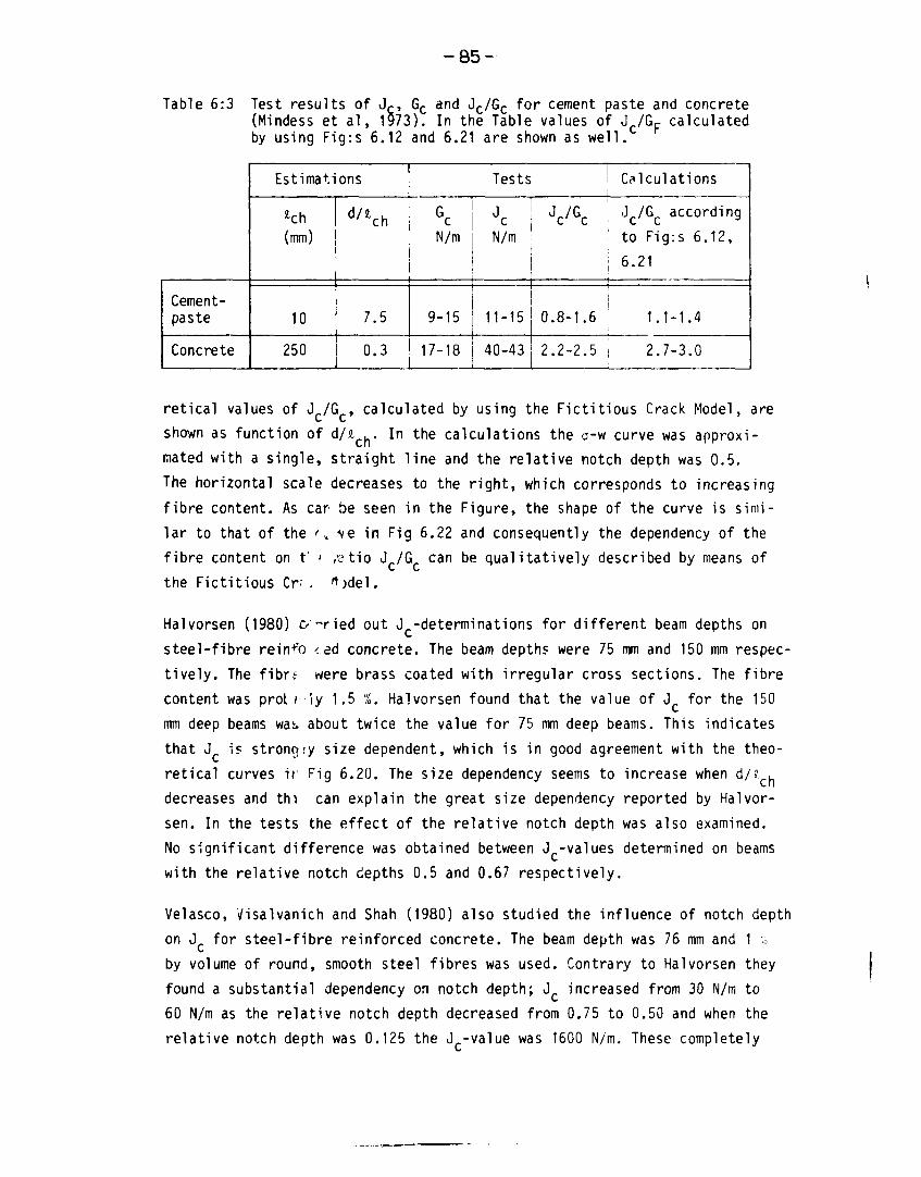
-85-

Table 6:3 Test results of Jc, Gc and Jc/Gc for cement paste and concrete(Mindess et al, 1973). In the Table values of J /Gp calculatedby using Fig:s 6.12 and 6.21 are shown as well.

Cement-paste

Concrete

Estimations

(mm)

10

250

d'*ch

7.5

0.3

Tests

GcN/m

, 1

9-15

17-18

JcN/m

i 11

11-15

40-43

Jc / Gc

0.8-1.6

2.2-2.5

Calculations

J /G according

to Fig:s 6.12,

6.21

1.1-1.4

2.7-3.0

retical values of J /G , calculated by using the Fictitious Crack Model, areshown as function of d/a , . In the calculations the o-w curve was approxi-mated with a single, straight line and the relative notch depth was 0.5.The horizontal scale decreases to the right, which corresponds to increasingfibre content. As car be seen in the Figure, the shape of the curve is simi-lar to that of the ' „ ve in Fig 6.22 and consequently the dependency of thefibre content on t' < ,-atio Jc/G can be qualitatively described by means ofthe Fictitious Cr . Ijdel.

Halvorsen (1980) &"ried out J -determinations for different beam depths onsteel-fibre reinfo < ed concrete. The beam depths were 75 mm and 150 mm respec-tively. The fibre were brass coated with irregular cross sections. The fibrecontent was prot r-iy 1.5 %. Halvorsen found that the value of J for the 150mm deep beams wa^ about twice the value for 75 mm deep beams. This indicatesthat J is stronojy size dependent, which is in good agreement with the theo-retical curves if Fig 6.20. The size dependency seems to increase when d/?.decreases and thi can explain the great size dependency reported by Halvor-sen. In the tests the effect of the relative notch depth was also examined.No significant difference was obtained between J -values determined on beamswith the relative notch depths 0.5 and 0.67 respectively.

Velasco, Visalvanich and Shah (1980) also studied the influence of notch depthon J for steel-fibre reinforced concrete. The beam depth was 76 mm and 1 »by volume of round, smooth steel fibres was used. Contrary to Halvorsen theyfound a substantial dependency on notch depth; Jc increased from 30 N/m to60 N/m as the relative notch depth decreased from 0.75 to 0.50 and when therelative notch depth was 0.125 the J -value was 1600 N/m. These completely

- 8 6 -

0.5

Fig 6.22 Jc/G as function of fibre content for a type of fibre-reinforcedconcrete (Mindess et a l , 1973).

10

|o/d»0Tl

1 0.5 0.2 0.1 0.05

Fig 6.23 Theoretical values of J /G as function of d/t .. Jr/G is calcula-ted ace. to Fig:s 6.12 3ndc6.21. The relative fiBtch depth is 0.5.

-87-

different results between two, fairly similar tests seem a little confusing.

One explanation could be the difficulties in finding the position of the

fracture load on the load-deflection curve, which is demonstrated in Fig 6.24.

In the Figure typical load-deflection curves according to Velasco et al are

shown for different relative notch depths. As can be seen in the Figure, there

is a long horizontal part of the curves close to the fracture load and only a

small, local variation of for example the fibre distribution can considerably

change the position of the fracture load. In the Figure the positions of the

fracture loads according to Velasco et ai are shown. If other positions were

chosen, which may be motivated at least where the deeply notched beams are

concerned, then the J -values would be completely different.

[x = peak point]

a=19mm

a=38

a=57

200 400 600 800 1000

6(jLim)

Fig 6.24 Load-deflection curves for different relative notch depths for aquality of steel-fibre reinforced concrete (Velasco et al , 1980).

According to the calculations; the test results and the discussion above it

seems unsuitable to use J as a fracture criterion for cement<tious materials

of normal dimensions. J is too dependent on specimen size, notch depth and

the shape of the -r-w curve for it to be useful. Also the difficulties of eva-

luating J , especially for fibre-reinforced materials, from the load-displa-

cement curve makes the parameter unsuitable.

-88-

6.4 The crack opening displacement approach (COD)

The fracture zone is able to transfer stress as long as the widening of thezone is less than a critical value w (see Fig:s 6.1-6.4) but when this valueis reached a real crack starts propagating. COD corresponds to the wideningof the fracture zone at the crack tip. If CODC is used as a criterion for theinitiation of real crack propagation then it equals w and consequently CODis then a material property. However, as discussed before, it is the fractureload and not the initiation of crack growth that is the most interesting thingto study and then, when used as a criterion for the fracture load, COD is

CODc/wc

1.0

Q5

0.2

0.1

0.05

0.25,

0.05 0.1 0.2 0.5d/l,

10ch

Fig 6.25 Theoretical values of C0Dc/wc as functions of d/£cn for the fourmodel materials in Fig:s 6.1-6.4. The curves are relevant forthree-point bending where the relative notch depth is 0.25.

- 8 9 -

normally an approximation. In Fig 6.25 theoretical values of iOD_.,<wr are snoun

as function of d/; , for the four node! materials presented in cig:s 6.1-6.4.

COD is determined at the maximum load. The curves are relevant for three-

point bending on beams with the relative notch depth 0.25.

Where materials with o-w curves according to Dugdale are concerned, a real

crack starts propagating when the fracture load is reached and consequently

then COD /w always equals unity. This is probably the explanation for the

fact that the COD-approach has sometimes been successfully applied on metals,

which often have i-w curves according to Ougdale. For most cementitious mate-

rials the j-w curve is quite different and then the COD-approach is less use-

ful, which can be seen in the Figure. COD increases greatly with increasing

values of d/i , and the more the shape of the J-W curve deviates from theen

shape according to Dugdale, the less the applicability of the COD-approach is.

Other calculations, which are not presented here, imply that COD is also

slightly affected by the relative notch depth; the applicability of the COD-

approach decreases with increasing relative notch depth.

The only application of the COD-approach to cementitious materials found in

literature was published by Valesco, Visalvanish and Shah (1980). They deter-

mined COD at the fracture load for fibre-reinforced concrete (round, smooth

steel fibres) and among other things they studied the influence of the rela-

tive notch depth. It is difficult to measure the displacement at the notch

tip so they measured the Crack Mouth Displacement (CMD) instead, i.e.the

displacement at the base of the notch and then they theoretically converted

the CMD -values to COD -values.C C

Velasco et al found that COD was dependent on the relative notch depth; it

decreased greatly with increasing relative notch depth. The same tendency,

but less pronounced, can be found from calculations according to the Ficti-

tious Crack Model. The very strong influence of the relative notch depth on

COD reported by Velasco et al may be due to technical proDlems when evalua-

ting the tests as it is very difficult, exactly as when determining the J-

integral for fibre-reinforced materials, to define the position of the peak

load on the load-displacement curve. However, it seems as COD , determined

at the fracture load, is too dependent on specimen geometry and the shape of

the o-w curve to be useful as a fracture mechanics parameter where cementi-

tious materials are concerned.

- 9 0 -

6.5 R-curve analysis

When calculating the resistance to crack growth it is necessary to know theactual crack depth (see 2.3.5), i.e.the notch depth (a) + the crack advance(aa) and consequently the position of the crack tip has to be well defined.This is the case for metals which normally have a small fracture zone but forcementitious materials it is much more difficult to define the position ofthe crack front;should it be at the tip of the fracture zone, at the tip ofthe real crack (i.e. a crack with no stress-transferring capability) or some-where in between? As the depth of tlie zone is often great, the definition ofthe position of the crack tip is of considerable importance.

A number of different methods for detecting the crack tip are reported inliterature. Welsh and Haisman (1969) used the compliance technique (complian-ce=deflection/load). In this method the initial compliances of notched beamswith different notch depths are first determined which makes it possible tofind a relation between compliance and notch depth. Then a notched beam isloaded to a certain point of the load -deflection curve. The secant modulusof this point is compared with the compliance curve and thus the actual crackdepth can be estimated. However, this method can only be used if the depthof the fracture zone is small as otherwise the fracture zone affects the comp-liance of the test beam but not the compliance curve. Therefore for cementi-tious materials, with large fracture zones, this method ought to be unsuitable.

The positition of the tip of the visible crack is probably the most natural de-finition of the location of the crack tip but this location is affected by themethod of observation; by the naked eye, by magnifying glass or by microscope.Strain measurements, acoustic emission measurements and other methods can alsobe used but the different ways of observing the crack tip give different crackdepths (cf Sok, Baron and Francois, 1979) and consequently different Kp-curveswhich is shown in Fig 6.26. In the calculations of the curves the positionof the crack tip was defined as the point where the widening of the fracturezone exceeds a critical value and the curves in the Figure represent differentcritical values ranging from 0 to 100 pm. The curves are relevant for three-point bending on beams with the relative notch depth 0.25 and the o-w curveis approximated with a single, straight line. Gr is chosen to 75 N/m, f^ to3 MPa and E to 30,000 MPa, which means that a real crack starts propaaatingwhen the widening of the fracture zone reaches 50 um.

As can be seen in the Figure, the curves become quite different for differentdefinitions of the position of the crack tip. When the critical value of the

-91 -

KR(MN/m/2)

1 s

50

100

100

ft = 3MPaE =30,000 MPaGp=75N/md=0.4ml=1.6ma/d = 0.25

• peak load

200Aa(mm)

Fig 6.26 Theoretical Kp-curves for three-point bend tests on notched beams.The J-W curve is approximated to a single, straight line. In the cal-culations the position of the crack tip was related to a criticalvalue of the opening of the fracture zone and the six curves are re-levant for different critical values ranging from 0 to 100 um.

fracture zone is zero this corresponds to the tip of the fracture zone. Thisposition can perhaps be roughly detected by means of acoustic emisson measure-ments or also by strain measurements. bO um correspond, in this case, to thetip of the real crack and consequently 10 um and 20 um represent positionssomewhere in the fracture zone. It ought to be possible for the naked eye toobserve "cracks" when their width exceeds about 25-50 um, compare Chapter 5.

In the Figure the positions of the peak loads are shown for the curves repre-

senting the three smallest critical values of the widening of the fracture zone.

As can be seen KR increases also after the maximum load is reached. In the

case of the curves representing the two largest critical values of the wide-

ning of the fracture zone the defined crack will not propagate until after

the maximum load is reached.

-92-

In Fig:s 6.27-6.30 calculated KR-curves for three-point bending are presen-ted. In the calculations the position of the crack tip was defined as thepoint where the widening of the fracture zone equals 10 urn.

For Fig:s 6.27-6.28 the o-w curve is approximated with a single, straightline and the material properties, which are given in the Figures, representa normal concrete quality. In Fig 6.27 KR-curves for different relative notchdepths are presented and, as can be seen, the curves are just very slightlyaffected by the relative notch depth. However, for different beam depths,see Fig 6.28, the curves are very different and this implies that the KR-cur-ve is not useful as a material property for concrete.

For Fig:s 6.29-6.30 the u-w curve is approximated according to Fig 6.4. With

the actual material properties the material should then correspond to a fibre-

reinforced concrete with a low percentage of short fibres. Also where this

material is concerned the curves are strongly affected by the beam depth whi-

le the influence of the relative notch depth is less pronounced.

The only example found in literature regarding KR-curves determined on bent

beams of unreinforced cementitious materials was presented by Brown (1972).

He determined KR-curves for mortar and used the compliance technique, though

somewhat modified, to find the actual crack depth. The tests were performed

on 38 mm deep beams and the relative notch depth was 0.5. The results for 6

individual beams are presented in Fig 6.31.

The KR-values are low which is probably due to the small specimen size but

perhaps also to the method of determining the actual crack depth. However,

the shapes of the curves are similar to those presented in Fig:s 6.27-6.28;

the curves first increase with increasing crack advance until they reach a

maximum and then they decrease.

Sok, Baron and Francois (1979) used very large double cantilever specimens,

see Fig 6.32, in order to determine KR-curves for concrete. Prestressed re-

inforcement was used parallel to the crack propagation path. This reinforce-

ment is probably necessary as it prevents crack propagation perpendicular to

the crack due to the high bending stresses. Such cracks in fact were also

reported for the reinforced specimens (Sok, 1978) but they were stopped be-

fore they reached the reinforcement. These side cracks and probably also the

reinforcement may affect the results.

The thickness of the specimen was reduced to one third along the crack propa-

-93-

K_ (MN/m3/2)

2

1

| G-W:(SL) 1

1

a/d =0.1

ft = 3 MPaE - 30,000 MPaGp=75 N/mtch = 0.25 m

d = 0.2 m

50 100 Aa(mm)

Fig 6.27 Theoretical Kn-curves for different relative notch depths. Thecurves are relevant for a normal concrete quality.

KR(MN/m3'2)

0.05

1C-W=(SL)1

ft=3MPa

E =30,000 MPaG =75N/m

lch=0.25 m

a/d=0.25

50 100 Aa(mm)

Fig 6.28 Theoretical Kp-curves for different beam depths. The curves arerelevant for a normal concrete quality.

- 9 4 -

KR(MN/m/2)

la-w:(FRC)l

a/d=0.1

ft =3 MPa

E=30,000 MPö= 1075 N/m

lch= 3.58 m

d = 0.2rn

50 100 Aa(mm)

Fig 6.29 Theoretical Kp-curves for different relative notch depths. Thecurves represent a fibre-reinforced concrete with a low percen-tage of short fibres.

KR(MN/m3/2}

lff-W:(FRC)l

d=CU

ft = 3 MPaE =30,000 MPa(3^=1075 N/m

tch= 3.58 ma/d = 0.25

50 100 Ao(mm)

Fig 6.30 Theoretical KR-curves for di f ferent beam depths. The curves representa fibre-reinforced concrete with a IJW percentage of short f ibres.

- 9 5 -

KR(MN/m'2)

0.7

OJB

0.5

0.6

03

2| cast notches

notchesd=38mma/d^O.5

1 1 I I I

0 2 ^ 6 8 10 12 U 16Aa(mm)

Fig 6.31 KR-curves for six mortar beams (Brown, 1972).

1100 mm

Prestressed reinforcement

9 ©

C-C

Fig 6.32 Double cantilever specimen used by Sok et al (1979) for determina-tion of K^-curves for concrete.

- 9 6 -

gation path. This varying thickness disturbs the stress distribution aroundthe fracture zone. The fracture mechanics properties of the specimen are al-so markedly affected. The formal tensile strength is reduced to one thirdin the zone where the crack propagates and so is the fracture energy. Thismeans that the i . -value formally is increased three times and consequently,according to the results in Chapter 5, the depth of the fracture zone is mar-kedly increased compared with the depth of the fracture zone in a specimenwith constant thickness. According to the discussion above, this type ofspecimen seems unsuitable for fracture mechanics tests on cementitious mate-rials.

In Fig 6.33 experimentally determined Kq-curves for different relative notchdepths are shown for a fibre-reinforced concrete with 1 % round, smooth steelfibres distributed at random (Velasco, Visalvanich and Shah, 1980). The cur-ves are determined on 76 mm deep beams in bending. In the Figure theoreticalcurves calculated by using the Fictitious Crack Model are presented as well.In the calculations a simplified a-w curve according to Fig 6.34 was used,which seems suitable for this material (Hillerborg, 1980). In Fig 6.34 an ex-perimentally determined (Petersson, 1980a) a-w curve is also shown and theagreement between the theoretical and the experimental curves seems good.The Young's modulus is 30,000 MPa and tne matrix crack is assumed to becomevisible when the widening of the fracture zone exceeds 10 utn.

As can be seen in Fig 6.33 the differences between the theoretical curves fordifferent notch depths are small. From experiments it is probably very diffi-cult to separate these curves and this explains the good agreement betweenthe experimentally determined Kq-curves. However, when the beam depth increa-ses, the slope of the theoretical Kq-curve decreases significantly and thisimplies that the Kq-curve cannot be used as a material property for this ma-terial either.

Kq-curves for an asbestos-cellulose cement composite have been determinedby Mai, Foote and Coterell (1980). They studied the influence of beam depthon the Kq-curves and used beam depths between 25 and 200 mm. The relativenotch depth was 0.3. The material contained 8 % asbestos fibres and 7 %cellulose fibres.

In Fig 6.35 the determined Kq-curves for the greatest and the smallest beam

depths and corresponding calculated curves are presented. In the calculations

it was assumed that the cellulose fibres did not affect the material parame-

- 9 7 -

(MN/m2)

15

o

—o—a = 9.5 rnm—•—a = 19 mm d=76mm

i —O-a = 38 mm

o

o

= 152mma= 38 mm

10 20 30 40 50 Aa(mm)

Fig 6.33 Experimentally (dots) and theoretically (lines) determined Kc-cur-ves for fibre-reinforced concrete with 1 - round, smooth steelfibresdistributed at random. During the calculations the .-w curvewas approximated according to Fig 6.34.

ff(MPa)

Thcor.Exp.

03 0.5w(mm)

Fig 6.34 Experimentally and theoretically determined o-w curves for a qua!i•ty of fibre-reinforced concrete with 1 of round, smooth steelfibres distributed at random.

- 9 8 -

ters very much and f^, E and 6p were chosen according to Table 6:2, which

means 9 MPa, 17,000 MPa and 1,500 N/m respectively.

KRlMN/m'2)

ds200mm

la/d-0,3|

10 20 30 50 60 Aa(mm)

Fig b.35 Experimental (dots) and theoretical (lines) Kn-curves of a qualityof asbestos-cellulose cement composite for different beam depths.The experiments were carried out by Mai et al (1980).

The 0-w curve was approximated according to Dugdale and the matrix crack was

assumed to become visible when the widening of the fracture zone exceeded

20 um.

As can be seen in the Figure, the beam depth markedly affects the Kq-curves.

This phenomenon is very well described by the theoretical curves calculated

by means of the Fictitious Crack Model, in spite of the simplified assumptions,

According to the calculations, the test results and the discussion above itseems unsuitable to use K^-curves as material properties for cementitiousmaterials, at least for normally used dimensions. The curves are too depen-dent on the specimen dimensions and the notch depth.

6.6 Conclusions

The fracture zone significantly influences the fracture process of cementi-

tious materials. The use of a single parameter seems insufficient for descri-

bing the complicated properties of the fracture zone and this explains why

99 -

the fracture mechanics approaches described above se^m unsuitable. '.%hf-n tr.e

Fictitious Cra>. k Model is used, the properties of the fracture ^one a<~(j desc-

ribed by the ;-w curve and therefore this mode 1 offers a nuch more realistic

and therefore better way of analysing the fracture process of cement itious

materials than approaches normally used. Even if very simplified assumptions

are used it is possible, by usi»"q the Fictitious Crack Model, to find out the

limitations of the G-, J-, COD- and R-curve approaches where cenentitious ma-

terials are concerned.

- 1 0 1 -

7 APPROXIMATIVE DETERMINATION OF THE ,•- AND --w CURVES

7.1 Introduction

When using the Fictitious Crack Model it is necessary to know the •- a-d -w

curves for the material. If the .---.-. curve is approximated with 5 single,

straight line, the curve is defined by the Young's modulus a-id tne tensile

strength. The ;-w curve is, if the shape of the curve is knew., defined 5/

the tensile strength and the fracture energy, see Fie 4.10. [r this Cha-jter

suitable methods for the determination of these prooerties ar^ discussed arå

test results for a number of concrete qualities are also presented. :-s "ice

or less standardized test methods already exist for the deterioration of the

tensile strength and the Young's modulus, most of the work is concentrated '>n

test methods by which the fracture energy can be determined.

7.2 Determination of the tensile strength (f\) on prismatic specimens

7.2.1 Introduction

The main difficulty in carrying out direct tensile tests for concrete and

other non-yielding materials on prismatic specimens is to achieve a uniform

tensile stress across a section of the specimen, without inducing stress

concentrations of too high a magnitude elsewhere. When the specimen is adao-

ted to the testing machine by ordinary clamping grips, the grips give rise

to stress concentrations and multiaxial stresses and the measured strength

becomes less than the real tensile strength. By using sophisticated clamping

grips (cf Johnston and Sidwell, 1968) the stress concentrations can be reduced

but probably not eliminated. A way of attaching the specimen at the ends is

to use an adhesive (Hughes and Chapman, 1965; Kadlecek and Spetla, 1966).

However, the adhesive and the concrete normally exhibit different lateral

strains when subjected to uniaxial stress due to their differences in Young's

modulus and Poisson's ratio. Thus, shear stresses are produced between the

two materials and in the region of the interface a principal stress lhat is

greater than the axial tensile stress is then introduced, which most likely

causes the fracture to occur at this interface. When using wet specimens it

is also difficult to obtain a sufficiently strong joint. Consequently, when

using ordinary clamping grips or adhesives, it is necessary to use necked

specimens. A necked specimen has a varying cross sectional area, which is

smallest at the middle of the specimen.

In order to avoid direct tensile tests it is customary to carry out indi-

-102-

rect tests, i.e. bend tests or splitting tests. However, these tests are great-ly affected by specimen dimensions and are therefore unsuitable. In Fig 7.1it is shown how the flexural tensile strength (fJ depends on the ratio beamdeptii/characteristic length (d/«, . ). The curves represent theoretical values,calculated by means of the Fictitious Crack Model, for wet specimens and spe-cimens subjected to a certain degree and distribution of shrinkage stressesrespectively, see below, and the dots represent test results. In the calcula-tions the a-w curve was approximated with a single, straight line. Similarresults, for both bend tests and splitting tests, are presented in the lite-rature (Wright, 1952; Mayer, 1967; Sabnis and Mirza, 1979; Modéer, 1979).

Vft

2 -

1

o wetv dried

0.1 0.3 10

Fig 7.1 Flexural tensile strength/tensile strength {fJf^) as a functionof beam depth. The curves are calculated by means of the FictitiousCrack Model and the dots represent test results.

Some comments ought to be made about the results shown in Fig 7.1. The resultsare relevant for three-point bending and the flexural tensile strength iscalculated as:

ff = (7:1)

where Fc = maximum load, i - beam length, b = beam width and d = beam depth.

This means that the influence of the transverse forces are ignored. This in-

-103-

fluence increases as the ratio beam length/beam depth decreases (Pfeiffer,1968) and the flexural tensile strength calculated by use of (7:1) is alwayssomewhat higher than the tensile strength. When the ratio beam length/beamdepth is as high as 4, this influence is small but it explains why the un-broken curve in Fig 7.1 tends towards a value, which slightly exceeds unitywhen the beam depth increases. The disturbance cf the stress field around theposition of the applied load probably also affects the results slightly.

When calculating the curve representing beams subjected to drying shrinkage

stresses, the stress distribution according to Fig 7.2 was assumed. In rea-

lity the distribution of course is much more complicated and affected by, for

example, drying time and changes in the environmental climate. The intensity

of the shrinkage stresses shown in Fig 7.2 produced the best agreement with

test results.

Os=f, Os-0.5ft

Fig 7.2 The shrinkage stress distribution used in the calculations in Fig7.1. o = shrinkage stress.

The tests were carried out on beams with square cross sections. The dryingvelocity was assumed to be proportional to the square of the beam depth(Hillerborg etal ,1977) and the beams with the depths 40, 80 and '60 mm weredried for 6, 24 and 96 h respectively. The specimens were dried on all sur-faces which means that the stress distribution in the specimens became diffe-rent compared with the distribution shown in Fig 7.2. The material used in thetests was a mortar (water-cement-ratio=0.65, maximum aggregate particle size=4 mm) and the z . -value was assumed to be 150 mm.

In spite of the simplified assumptions the agreement between the calculatedcurves and the test results is good and it seems possible to describe the bendtest or, unnotched specimens by use of the Fictitious Crack Model. Among other

things it can be noticed in Fig 7.1 that the dependency of the beam depth on

the flexurai tensile strength increases when the specimen becomes subjected

to shrinkage stresses.

7.2.2 Direct tensile tests on prismatic specimens

In Fig 7.3 and Fig 7.4 a new type of grip is presented by which it is possib-le to determine the tensile strength by direct tests on prismatic specimens.The grip consists of steel plates on to which wedge-shaped rubber inserts areglued. It is essential that the inserts are oriented according to Fig 7.3.

O

Ifife

Fig 7.3 Grips for direct tensile tests.The wedge-shaped rubber insertsreduce the stress-concentrationsto a minimum.

Fig 7.4 Tensile test using thegrips in Fig 7.3.

-105-

Each part of the grip is pressed against the specimen at two points; one force

near the end of the specimen and one lesser force close to the free part of

the specimen.

The advantages of these grips compared to ordinary grips may be summarized as

follows:

1. The clamping forces are greatest at the ends of the specimen and

least at the ends of the grips close to the middle of the specimen.

This means that the stress perpendicular to the tensile direction

is small at the most critical cross section, i.e. at point A in

Fig 7.3, and at this point the stress field becomes almost one di-

mensional .

2. Due to the variable stiffness of the wedge-shaped rubber inserts,

the main part of the load is applied close to the ends of the spe-

cimen and consequently the axial stress grows gradually to its maxi-

mum value, which is shown in Fig 7.3.

3. The loading force at one point gives rise to a non-uniform stress

distribution over the corresponding cross sectionol area. The stress

distribution becomes more uniform at a distance from the loading

poifft. As the main part of the loading forces acts close to the ends

of the specimen, the stress distribution becomes fairly uniform at

the end of the grips. Consequently, the stress concentrations at

point A become reduced to a minimum.

4. These grips make it possiblv to use prismatic specimens,which faci-

litate the manufacturing of te?t pieces. Specimens can also be sawn

out from a structure.

The tensile tests presented in 7.5 below were carried out on 177 specimens.

The fracture location distribution for the specimens examined in the test

program is shown in Fig 7.5. The fracture location is defined as the distance

between the position of the fracture load and the centre of the specimen.

In the Figure the position of the clamping grip is shown. Ac indicated in the

Figure, the rubber insert deforms as the specimen becomes loaded and the con-

tact between the insert and the specimen is lost over a distance of about .70

mm at the thick end of the insert and consequently the free part uf the spe-

cimen increase*',, in this c a •,<.*. f'roi;i '''*'<) to about 1i"'O IMM in the '.t- t.

-106-

Number of fractures

t30-

20-

10

Centerspecimen

End ofspecimen

160 mm

Fig 7.5 The fracture location distribution for the 177 direct tensile tests.

As can be seen in the Figure, the fracture locations are well distributedover the length of the free part of the specimen, which implies that no stressconcentrations or multi-axial stresses affect the distribution and thus thefracture load. Of course there are a few fracture locations outside the freepart of the specimen but this is quite natural due to the varying tensilestrength along the specimen for an inhomogeneous material such as concrete.

The tensile strength determined by use of the grips described above has beencompared with the flexural tensile strength for a number of concrete qualities(Petersson, 1981 and 7.5.5 below) and the ratio ff/f+ seems to agree well withtheoretical relations, which also implies that the grips are suitable for de-termining the direct tensile strength on prismatic concrete specimens.

-107-

7.3 Determination of the Young's modulus (E)

The static Young's modulus is a well defined material property for linear

elastic, non-creeping materials only, otherwise the modulus is affected by,

for example, loading velocity, load intensity and the number of load cycles.

The dynamic Young's modulus (E.) on the other hand is a well defined mate-

rial property and for this reason it is the dynamic Young's modulus that has

been determined in this work. The dynamic Young's modulus is always higher

than the static Young's modulus, the difference is normally 10-20 (Bastgen

and Hermann, 1977).

In this thesis a method according to Vinkeloe (1962) has been used for deter-

mining the dynamic Young's modulus. The method is described briefly below.

According to Vinkeloe there exists a relation between the resonance frequency

of a beam and the dynamic Young's modulus that can be expressed as:

(7:2)

where f is the resonance frequency, M is the mass of the beam, .: is the beam

depth, T is a correction factor depending on the dimensions and the Poisson's

ratio, C is a constant depending on the mode of oscillation and I is the mo-

ment of inertia for the beam.

For the first mode of oscillation the beam will oscillate around two points,

which are located 0.224 i from each end of the beam. In the tests these loca-

tions should coincide with the position of the supports. For the first mode

of oscillation, which is used in this work, C is 3.56.

The dimensionless constant T is dependent on the Poisson's ratio and the ra-

tio K/j., where K for a beam with a square cross section equals beam depth/

yi2. In Fig 7.6 T is given as a function of K/f. when the Poisson's ratio is

0.167. However, the curve is very little affected by the Poisson's ratio,

for example, if Poisson's ratio is changed to 0, the value of T at K/"=0.1

decreases by 1.3 % and when K/e,-0.02 (which is the case at the tests presen-

ted in 7.5) T decreases by 0.4 .','.

In Fig 7.7 a schematic description of the test equipment used for determining

the dynamic Young's modulus is shown. The specimen (4) is oscillating due to

the vibrations caused by the vibrator (3). The frequency of the vibrator is

controlled by a tone generator (1) and a frequency counter (2). The vibrations

of the beam are registered by use of a pick-up (5) and an oscilloscope (6).

-108-

0.2 K/l

Fig 7.6 Correction factor T as a function of K/«:.

J)Q

Fig 7.7 Testing equipment for measuring the resonance frequency and theYoung's modulus on concrete beams. 1=tone generator, 2=frequencycounter, 3=vibrator, 4=specimen, 5=pick-up, 6=oscil1oscope.

- 1 0 9 -

The frequency is varied by use of the tone generator and the highest amplitude

registered on the oscilloscope gives the resonance frequency and thus the cy-

namic Young's modulus.

7.4 Determination of the fracture energy {&c)_

7.4.1 Introduction

The fracture energy (Gp) is defined as the amount of energy necessary to crea-

te one unit of area of a crack and the principle when measuring Gr is there-

fore to let a crack propagate a well defined distance and measure the energy

consumption due to the crack propagation. As discussed previously it is very

difficult to define the position of the tip of a propagating crack and for this

reason it seems necessary to measure the total energy consumption from the

start of crack initiation until the crack has propagated right through the

specimen as this gives a well defined length of the crack propagation path.

It is essential that the fracture, i.e. the crack propagation, is stable as

otherwise uncontrolled energy consumption due to dynamic effects will take

place and it is also essential that the energy consumption outside the fracture

zone is minimized. These problems are discussed in detail below.

There are a number of specimen types that can be used in order to obtain stable

crack propagation, for example double torsion specimen (cf Wecharatana and Shah,

1980), compact tension specimen (cf Hillemeier and Hilsdorf, 1977), double can-

tilever beam (cf Chhuy, Benkirane, Baron and Francois, 1981) and also direct

tensile test specimens (cf Evans and Marathe, 1968 and Chapter 8 below).

However, the most simple specimen that can be used is a notched beam and in

this case all the work is concentrated on the determination of the fracture

energy by the use of three-point bending on notched beams.

Very few results of the fracture energy determined from stable tests sre found

in literature. Moavenzadeh and Kuguel (1969) measured the energy under the

load-deflection curve for some qualities of cement paste, mortar and concrete.

They related this energy to the actual crack surface and not to the net cross

sectional area and therefore their results nust be considered as some form of

sjrface energies and ;iot as fracture energies. Shah and McGarry (1971) also

measured the energy under the load deflection curve and their results corre-

spond tc vaH.es of the fracture energy of 5-33 N/m for cement paste, 20-95 N/m

fo"1 mortar and 30-135 N/m for concrete. It is however doubtful if all their

— 110 —

tests were carried out in a stable manner and at the evaluation of the tests

the effect of the energy supplied by the weight of the beams was probably

not considered. Harris, Varlcw and Ellis (1972) found values of Gp for con-

crete of about 20-120 N/m but also in these tests it is doubtful if the ef-

fects of stability and energy supplied by the weight of the beams were con-

sidered. Modéer (1979) found Gp-values of about 10, 60 and 110 N/m for some

qualities of cement paste, mortar and concrete. These tests have been car-

ried out in a stable way and the tests v.ere, at least to some extent, com-

pensated for by the energy supplied by the weights of the beams. Fracture

energy tests have also been carried out on fibre-reinforced materials (cf

Harris, Varlow and Ellis, 1972; Ohigashi, 1978; Mai, 1979) but these results

are not discussed here.

Even if there are some results of the fracture energy determined on notched

beams, no investigations have been carried out in order to study the applicabi-

lity of the test methods and the usefulness of Gp as a material property. For

this reason the fracture energy and the usefulness of the three-point bend

test for determining Gp are dealt with in detail below.

7.4.2 Stability conditions for three-point bend tests on notched beams

In order to obtain a relevant value of the fracture energy from a three-point

bend test on a notched beam, the amount of energy supplied by the loading

force and the weight of the beam must equal the amount of energy consumed by

the crack propagation. This means that the energy consumption taking place

outside the fracture zone in front of the crack tip has to be minimized. To

fulfil this condition the fracture must be stable, otherwise energy consump-

tion due to dynamic effects will occur.

In order to obtain a stable fracture it is necessary to use a displacement

controlled testing machine as a load controlled machine always produces an

unstable fracture when the maximum load is reached. The crack must also,

for every point of the load-deflection curve, be able to consume the amount

of energy that is re.eased from the beam and the testing machine during the

deformation.

Cooper (1977) and Modéer (1979) calculated conditions of stability for three-

point bend tests on notched beams for the linear elastic case. According to

their results it is almost impossible to obtain a stable fracture for cemen-

titious materials unless the ratio notch depth/beam depth (a/d) is very large

-111-

and the test is performed in a very stiff testing machine. However, as dis-

cussed before, concrete is far from being an ideal linear elastic material

and below it is shown how this makes it much easier to fulfil the conditions

of stability.

In Fig 7.8 an example of a stable load-deflection curve (F-- curve) is shown

for a three-point bend test on a notched beam. The total amount of energy,

(L, necessary to deflect the beam a distance :. can be calculated from the

F-6 curve. Q h is affected by the strain energy release of the beam when the

crack propagates as well as the amount of energy consumed by the slow crack

propagation:

°1Q b = (7:3)

In the total test arrangement, the energy release and consumption of the tes-

ting machine must also be considered. The stiffness, k, of the testing machi-

ne is defined as:

L

Fig 7.8 A load-deflection curve for a three-point bend test on a notchedbeam. The energy consumption necessary to deflect the beam a dis-tance '\ is

6M

-112-

(7:4)

where F is the load applied to the testing machine and 6M is the deformation

of the testing machine due to the load F.

The stiffness of the testing machine determines the energy consumption of the

testing machine, QM, when the beam is deflected a distance 5:

F(6)6 2

In order to obtain a stable fracture, the derivative of the total energy con

sumption has to be positive for any value of 6:

. F(.) •££>!£>>„ (7:6)

(7:6) gives the condition of stability:

k > - ^ r ^ (7:7)

(7:7) implies that the stiffness of the testing machine has to be greater than

the steepest slope of the descending part of the F-6 curve, in order to obtain

a stable fracture.

By use of the Fictitious Crack Model, F-6 curves can be calculated for diffe-rent beam geometries and material properties. Conditions of stability canthen be derived from (7:7). Results from such calculations are presented inFig 7.9 b-f. In the calculations the a-w curve was approximated with a single,straight line (SL). In Fig 7.9a conditions of stability for the linear elasticcase according to Modéer (1979) are shown.

The geometrical parameters affecting the stability are i/ö, a/d and b (s.=beamlength, d=beam depth, b=beam width and a=notch depth). The material proper-ties affecting the stability, for a given shape of the a-w curve, are the cha-racteristic length (^cu) and the Young's modulus. The stability is also affec-ted by the stiffness of the testing machine (k). The energy stored in the machi-ne is directly proportional to E, b and 1/k and consequently directly propor-tional to Eb/k.

The curves in Fig 7.9 show that the conditions of stability are strongly af-fected by the d/e.-value. A specimen of cement paste with a depth of 25 mm

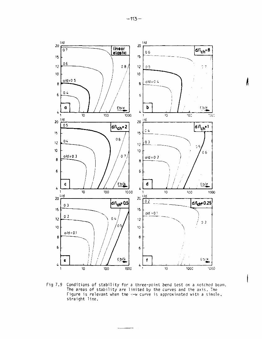
—113 —

20

15

12

10

8

l/d l/d

0 7 - - -

0.6

a/d = 0 51 —*.

a I

——.

1/linearclastic

0 8 /

j

1i l l 1

15

12

10

B

6

06

05^ -

o/d i 0 4 \

"^i /b

, / / /' ,

d/lch=8

/

: 7

15

n10

8

6

4

0.3" " — •

^ d = 0 ^ ^

\\

e /7i i i i

d/l^OSy

0A 1I hi

1/ / /' / / t.

20I/d

15 -

12

10

8

6

100 1000

02

o / d = 0 1

-

-

f

\

1

i l l i

d/ldfO.25

1/ 0 3

Eb/k

10 100 1000 10 1000 1000

Fig 7.9 Conditions of stability for a three-point bend test on a notched beam.The areas of stability are limited by the curves and the axis. TheFigure is relevant when the n-vt curve is approximated with a single,straight line.

l/d20

»5

12

10

8

6

a/d=0.5

[0.5)

0.3

\

1

; /

j

d/lch=8

j

i

/(0.7)

/

/ Eb/k

10 100 1000

l/d

15

12

10

8

6

k

a/d=0.1

-

-/

/ // /

(0.3)/ /, / /

d/irt-i

0.3 1 // /(0.5)

I'j // /

/ Xs1 /

ll /Eb/K1

t/d

10 too 1000

20

15

12

K3

8

(0.3)

(0.1)

/

/

d/lch*O5

J;/(0.5)

/

Eb/k^

10 100 1000

Fig 7.10 Conditions of stability for a three point-bend test on a notchedbeam. The curves are relevant for a two line approximation of the0-w curve according to Fig 6.3 (unbroken lines) and the curves arecompared with the results in Fig 7.9 (dashed lines).

- 1 1 5 -

has a d/x..-value of about 2-4. Although this material is normally conside-

red to be very brittle, the curves of stability noticeably differ from those

calculated with the assumption of a linear elastic material. A concrete spe-

cimen with a depth of 50 mm has a A/i . value of about 0.2. As seen in the Fi-

gure, these curves differ completely from the linear elastic case and the con-

ditions of stability according to the linear elastic case are much too hard

for concrete.

When determining Gp, all the beams have to fail in a stable manner, otherwise

a systematic error will occur. When using the mean value of d/>' . about 50

of the beams will fail in an unstable manner. This is a reason why the d/. . -

value ought to be increased somewhat before using Fig 7.9.

In Fig 7.10 conditions of stability are shown for three different values of

6/i , when the o-w curve is approximated with two straight lines according

to Fig 6.3 (unbroken lines). The dashed lines correspond to the results in Fig

7.9. As can be seen, the conditions of stability are considerably harder for

the single line approximation of the o-w curve than when the curve is approxi-

mated with two straight lines. This can be explained by the fact that the les-

ser the slope of the o-w curves is directly after the maximum stress, the

higher the fracture load becomes and, for the same value of G-, the steeper

the descending part of the load-deflection curve becomes, compare Fig 6.5.

However, as the conditions of stability in Fig 7.9 are on the safe side, they

can normally be used for concrete and similar materials, especially as the con-

ditions are relatively mild. For example, for a concrete beam with the dimen-

sion 100 x 100 x 1000 mm and the relative notch depth 0.5, the stiffness of

the testing machine has to exceed about 10,000 N/mm in order to obtain a stable

fracture (>, . and E are assumed to be 200 mm and 40,000 MPa respectively). Most

modern testing machines fulfil this condition. Where fibre-reinforced materials

are concerned other conditions of stability naturaUy have to be used but these

materials normally have such high :•. ,-values that there are no problems in

achieving stable fractures.

7.4.3 Evaluation of the Gp-test

When carrying out stable three-point bend tests, energy is not only supplied

by the load but also by the weight of the beam. The effect of the energy supp-

lied by the weight of the beam can be eliminated if the length of the beam is

twice the distance between the supports according to Fig 7.11a. Of course shor-

ter beam lengths can be used if the moment caused by the weight of the beam is

compensated for by weights at the ends of the beam dccordinq to Fig /.lib.

- 1 1 6 -

(Specimens according to Fig 7.11 are here called compensated beams). If this

method is used then the fracture energy is directly obtained as:

^ T (7:8)

where A = the area under the stable load-deflection curve, d=beam depth,a=notch depth and b=beam width.

a),'777777 i>rn>>

^ 1/2

b)I

i)r7)) rfnv

Fig 7.11 a) The energy supplied by the weight of the beam can be compensatedfor by using a beam with the length equalizing twice the dis-tance between the supports

b) The energy supplied by the weight of the beam can also be com-pensated for by using weights at the ends of the beam.

When using the methods described in Fig 7.11 for evaluating Gp, some problemsmay arise. The beams have to be long which can give rise to problems in theperformance of the test. Another problem is that there will be a long "tail"on the load-deflection curve,see Fig 7.12. Theoretically this tail will be in-finitely long. The area under the curve is preferably measured by using a pla-nimeter and then the long tail can cause problems. A small fault in the balan-ce of the system can also give rise to substantial errors due to the long tail.For these reasons it would be better if the test could be stopped at a certainmoment but this is only possible if the effect of the weight of the beam canbe estimated.

- 1 1 7 -

Fig 7.12 A load-deflection curve for a stable three-point bend test on anotched beam. The shaded area (A.) defines the area under the load-deflection curve if there is no compensation for the energy suppliedby the weight of the beam.

If there is no compensation for the effect of the weight of the beam, i.e. an

uncompensated beam, then the beam will fail at a point corresponding to the

load F on the compensated load-deflection curve, see Fig 7.12. F can be found

by equating the moment due to F and the moment due to the weight of the beam:

ol _ mgjr1

r _

o "7:9!

where m = weight per unit length of the beam, M = weight of the beam (between

the supports) and g = 9.81 m/s .

When using the uncompensated beam for determining GF the area under the load-

deflection curve corresponds to the area A. in Fig 7.12. This method is use-

ful only if it is also possible to estimate the energies corresponding to

- 1 1 8 -

A?> A., and A, in the Figure. Normally A- is so small (less than 1 - 2 * of

the total area) that it can be neglected. The area A- equals F 6 (where 6is the deflection at the final fracture of the uncompensated beam) and con-sequently:

Mga,(7:10)

For small values of the load (on the descending part of the curve) it is fairto assume that the beam is divided into two rectangular pieces which are onlyconnected by the fracture ;.one, see Fig 7.13. It is assumed that the sides ofthe crack and the fracture zone are plane and that the compression zone is con-centrated on a point at the top of the beam. This of course is an approximationas there always exists a compression zone at the top of the beam. However, itcan be shown that the discussion below is relevant also when there exists acompression zone if the stress distribution over the remaining ligament isassumed to be uniformly changed as the depth of the fracture zone decreases.

For a given beam according to Fig 7.13 and defined material properties thedepth of the fracture zone (dp) is, when a real crack has started to propa-gate, reciprocally proportional to the deflection of the beam (ö), i.e.:

dF = -1 (7:11)

where C is a constant. Both the total closing force and the moment arm areproportional to dp and consequently:

Fig 7.13 An approximative description of the last phase of a stable three-point bend test.

- 1 1 9 -

F(5) = -4 (7:12)5

where Z^ is a constant. The area A^ in Fig 7.12 then can be calculated as:00 ut

A3 =

s 5 00 0

and consequently, according to (7:9) and (7:12):

A> = - ^--]r>

This means that the value of A^ equals k? anc'' w^en usin9 the uncompensatedbeam, the expression for Gp is:

In order to study the relevance of (7:14), tests were performed on beams wherethe effect of the weight of the beam was compensated for by using weights ac-cording to Fig 7.11b. The total area under the load-deflection curve was deter-mined and F was calculated by use of (7:9). After this the areas A ^ A^, A3

and A- according to Fig 7.12 could be determined and then the results derivedfrom (7:14) could be compared with the true values determined by use of (7:8).

Two different beam depths were used, 50 mm and 200 mm respectively. The widths

were 50 mm and the relative notch depths 0.5 for all the beams. Cast notches

were used for the 200 mm deep beams and sawn notches for the 50 mm deep beams.

The widths of the notches were 4 mm.

The mix proportions of the concrete used in the tests are presented in Table 7:1

Tests wero performed for two different ages of the concrete, 7 and 28 days res-

pectively.

Table 7:1 Mix proportions for the concrete used for analysingdifferent evaluation methods of the Gp-test.

Cement (ordinaryWater

Aggregate 0-4 mmAggregate 4-8 mm

Portland)

(not crushed)

(crushed quartzi te)

367220837837

kg/m3

kg/m3

kg/m3

kg/m3

-120-

The 200 mm deep beams were cast in plywood moulds and the 50 mm deep in steel

moulds. The specimens were stored under wet sackcloth until the time for the

test and the beams were kept wet during the testing. The loading velocity was

chosen so that the maximum load was reached about 30 seconds after the test

started.

In Table 7:2 the results for all the beams are shown. Results representing four

alternative evaluation methods are presented. Alternative I corresponds to

the area under the load-deflection curve for the uncompensated beam, which

means that no corrections are made for the energy supplied by the weight of

the beam. Alternative II means that the area kr is included when calculating

Gp but not the area A-,. Alternative III corresponds to (7:14), which means that

both A,, and A-, are considered. Alternative IV represents Gr-values calculated

by use of the area under the load-deflection curve for beams where the energy

supplied by the weight of the beam is compensated for and these values can

therefore be considered to be true. In the last column of the Table the diffe-

rences between Alternative III and Alternative IV, calculated as ((Alt Ill-

Alt IV)/Alt IV) x 100 ',, are shown.

As can be seen in the Table the energy supplied by the weight of the beam af-

fects the results considerably. This is illustrated in Fig 7.14, where the

areas A^, A£, Aj and A^ are shown for two of the beams used during the tests.

For the 50 mm deep beam the Gp-value according to Alt I must be compensated

for by about 50-60 Z in order to correspond to the true value of Gp and for

the 200 mm deep beam the compensation has to be about 150-250 %\ However,

in spite of the great effect of the weight of the beam, the results according

to Alt III seem to be in good agreement with the true values. For the 21

50 mm deep beams there are only two Gp-values according to Alt III differing

from the true values by more than 5,2 ',» and the differences between the mean

values according to Alt III and Alt IV are only about 1 %. Due to the wide

scatter in the test results, these small differences can normally be neglected.

For the 200 mm deep beams the differences between the values according to Alt

III and Alt IV are naturally greater but they are still astonishingly small

compared with the great corrections that have to be carried out. No indivi-

dual corrected value differs more than 15 % from the true value, only 3 out of

12 differ more than 10 % from the true value and the two mean values differ

only by 7,8 I and 3,2 % respectively from the true mean values. The latter dif-

ferences are negative and would decrease to 6,4 % and 1,8 % respectively if

the area A^ was considered, see Fig 7.14.

-121-

Table 7:2 Gr values evaluated by using different methods.

Age

days

7

mean

7

mean

28

mean

28

mean

Beamdepth

mm

50

values:

200

values:

50

values:

200

values

Alt I

no cor-rectionGrV(d-a)b

62.056.247.953.248.065.463.760.246.177.8

58.0

44.233.031.423.224.236.8

32.1

6.565.285.464.763.858.170.258.380.758.255.2

65.9

41.536.744.247.036.438.2

40.7

GF(N/m)

Alt II

no cor-rection for

G3

Alt I I I

correctedfor weightof beamace. to

(6 -a ) l 2 I (7:14)j78.1 94.2

71.1 !', 86.062.5 '• 77.171.5 89.862.7 i! 77.487.583.878.861.697.0

75.5

85.964.367.2

119.6103.897.477.2

116.1

92.9

127.795.5

103.054.8 ; 86.454.273.4

66.6

80.5

84.2110.0

101.1

95.782.0 98.7

103.4 • 121.479.1 93.477.6 .: 91.478.6 • 99.189.0 . 107.874.8 91.3

100.2 119.773.1 , 88.0

, 75.4 ; 95.6

83.1 !i 100.2

89.1 : 136.6\ 73.6 ! 110.5

82.4 : 120.6: 84.8 ' 122.7i 70 .8 ; 105.2! 83.1 ;, 128.0

' 80.6 ! 120.6

Alt IV

true value

90.487.679.688.179.7

106.0101.0102.085.6

121.4

94.1

130.5101.4116.387.298.8

124.0

109.7

91.096.0

126.494.092.0

109.3107.090.7

114.090.3

101.1

101.0

138.2120.3119.0122.0114.4134.0

124.6

Di f fe rence betweena l t I I I and a l t IV

4.2-1 .9-3 .1

1.9-2 .9

3.42.8

-4 .5-9 .8-4 .4

-1 .3

-2 .1-5 .8-11.4-0 .9

-14.8-11.3

-7 .8

5.22.8

-4.0-0 .6-0.7-9 .3

0.70.75.0

-2.5-5 .4

-O.S

-1 .1-8 .2

1.30.6

-8 .0-4 .4

-3 .2

- 1 2 2 -

F(N)

0.03'/.

F(N)

d = 200mmage = 26 days

1.4% <${mm)

Fig 7.14 Illustration of the areas A,, Ap, A- and A4 for two beams used inthe tests. The curves correspond to beam depths of 50 mm (top)and 200 mm (bottom) respectively.

- 1 2 3 -

As i^ntioned before the evaluation method according to Alt III has some advan-

tages compared ^ith the evaluation method according to Alt IV; smaller speci-

mens can be usea and it is easier to measure the area under the load-deflec-

tion curve. As the differences between the results from the two methods are

so small, the test method according to Alt III, i.e. according :o (./:'-+/,

seems oreferable "in most cases.

7.4.4 Gp as a material property

A material property must fulfil two criterions; it must be independent, of r-:<o- '

ciiren geometry and it must be independent of the type of loadinq. h: order to

check whether the fracture energy fulfils these criterions, Gp-deturrrinationj

were carried out on four different specimen geometrias, see Fig 7.15, of whicn

two were subjected to three-point bending and tv.o to direct ten-ion.

The types of specimens denoted I and II are notched beams, which were tested

in three-point bending. The depths of the beams were 50 mm and;:0'Jmn respecti-

vely. These beams are in fact indentical to those used in the tests prosor, tec!

in 7.4.3, which means that the energy supplied by the weight of the bear< was

compensated for by using weights and Gp was evaluated by the use of (7.-;-:,.

The concrete quality used is shown in Table 7:1. The testing procedure xrA

the preparation of specimens are discussed in 7.4.3 but a few supplementary

comments have to be made. For both the beam dimensions the relative loading

velocity was the same, which means that the ratio load/maximum load as a func-

tion of the time was identical for the two types of beams. The maximum load

was reached about 30 seconds after the start of the test. Cast notches were

used for the 200 mm deep beams and sawn notches for the 50 <nn deep beans. w

cast notches are used, the material close to the notch tip will be disturbud

during the casting. This disturbance ought to affect the Gp-value more for

small beams than for large beams and for the 200 mm deep beams this inf

on the Gp-value is assumed to be small. When sawn notches arc used the>-i? is

no such disturbance of the material in front of the notch tip.

G,- was also determined by using completely different specimen types denoted

III and IV. The specimens were cast in steel moulds and were stored in the

same way as the beams until one day before testing. During the last day these

specimens were insulated with plastic foil and stored in the air.

By using the stiff tensile testing machine described in Chapter '6 stable ten-

sile tests were carried out on the two latter types of specimens. The area

under the load-deformation curve includes not only the amount of energy consu

- 1 2 / + -

I, II

Specimen ISpecimen II

d50

200

S500

2000

b5050

a25

100

III

20

50 H

T

50

Fig 7.15 The four types of specimens used in the tests. The dimensions aregiven in mm. S=length between the supports.

- 1 2 5 -

med by the fracture zone but also the amount of energy consumed by the material

outside the fracture zone before the tensile strength is reached, compare

Chapter 3. In order to obtain the energy consumed by the fracture zone, the

shaded area in Fig 7.16 must therefore be substracted from the total area un-

der the curve. The shaded area is defined by the increasing part of the a-r

curve and the unloading curve for the material outside the fracture zone. The

unloading curve is assumed to be parallel with the initial slope of the •:-••.

curve, compare 8.1. Gp then is calculated as the reduced area divided by the

cross sectional area of the specimen. The loading velocity was chosen so that

the maximum load was reached about 60 seconds after the start of the test.

All the tests were carried out on wet specimens, exactly the same as for the

beams.

The results are presented in Fig 7.17 and Fig 7.18. As can be seen in the Fi-

gures, the mean values of Gp for the 7 days old concrete varies between 86 N/m

and 109 N/m and for the 28days old concrete between 98 N/m and 124 N/m. These

variations must be considered as small, especially if they are compared with

the variations between the values of the critical strain energy release rate

(G ) for the same specimens, see Fig 7.19. The mean values of G vary between

3 N/m and 23 N/m for the different specimen geometries. The G -values are

calculated by use of ordinary linear elastic relations (of course there are

no G -values for the unnotched specimen as G is defined only for notched

structures) and E is assumed to be 30,000 MP , which ougth to be a normal va-

Fig 7.16 When determining Gp by using a stable tensile test, the energy con-sumption due to irreversible strains outside the fracture zone, i.e.the shaded area in the Figure, must be substracted from the totalenergy consumption.

- 1 2 6 -

G^IN/m)

125 -

100 -

75 -

50

25

bend testd=50mm

AGE-. 7days

o

• J .

J

I

8O

©O

IIt

-©-

III1

oo

IYJ 1

bend testd=200mm

tensile testunnotchedspecimens

tensile testnotchedspecimens

Fig 7.17 GF-values for a 7 day old concrete determined on different types ofspecimens. Each circle represents a single specimen and the dashedlines represent mean values.

lue of the static Young's modulus for this material. It can be noted that the

differences between the G -values for the different beam depths are in good

agreement with the calculation results presented in Fig 6.14.

According to these test results, Gp seems to be useful as a material propertyfor concrete and it is superior to the critical strain energy release rate.However, Gp seems to be slightly affected by the beam depth. There are somepossible explanation for this size dependency and one of these is that theenergy consumption outside the fracture zone due to the non-linearity of theo-e curve may affect the Gp-value more for deep beams than for low ones. Nor-mally the energy consumption outside the fracture zone is assumed to be negli-gible. In order to study whether this assumption is realistic or not, finiteelement calculations were carried out on notched beams with different beamdepths and the development of the stress field around the crack propagation

-127-

Gp(N/m)

125

100

75

50

25

- O

-f--

I

8

%

II

AGE: 28 days

0-o-

o

III

o

IY1 1

bend testd=50mm

bend test= 200mm

tensile testun notchedspecimen

tensile testnotchedspecimen

Fig 7.18 Gp-values for a 28 day old concrete determined on different typesof specimens. Each circle represents a single specimen and thedashed lines represent mean values.

path was registered during the propagation of the fracture zone. By comparingthe stress field with non-linear a-e curves for concrete, the energy consump-tion outside the fracture zone can be estimated. Of course more complicatednon-linear finite element calculations would give better results (the non-linear zone around the fracture zone would probably be slightly larger), butfor rough estimations the simple method described above ought to be useful.

The finite element mesh used in the calculations is presented in Fig 7.20.Due to the symmetry only half the beam had to be considered. The two beamsused in the calculations correspond to the beams used in the tests presentedabove (d x b x i = 50 x 50 x 500 mm3 and 200 x 50 x 2000 mm3, a/d = 0.5). Thecalculations were carried out by use of calculation method II (superposition),see 4.3, and in the calculations the o-w curve was approximated with astraight line.

Gc (N/m)

30

20

»0

i

bend testd=50mm

- 1 2 8 -

.O.

O

II

AGE: 28 days

E =30,000 MRa

•o

9

|

Hl

o

bend testd=200 mm

tensile testunnotchedspecimens

tensile testnotchedspecimens

Fig 7.19 Gc-values (critical strain energy release rate) for a 28 day oldconcrete determined on different specimen geometries. Each circlerepresents a single specimen and the dashed lines represent meanvalues.

The highest value of the first principal stress obtained in the calculationswas registered for each element. In Fig 7.21 lines connecting points with iden-tical maximum vaiues of the first principal stress are presented for the twobeam depths (observe the different vertical scales). The curves are obtainedby use of interpolation between the stresses in the middle of the elements.The results are relevant for a material with a i . -value of 250 mm, i.e. anormal concrete quality. The unbroken lines are calculation results, whilethe dashed lines are estimations. It is assumed that the extension of the non-linear tensile zone is zero at the top of the beam, which is explained by thefact that a compression zone must always exist in this region, even when thefracture zone has almost reached the top of the beam.

The results in Fig 7,21 are of interest only if they can be compared with a

.'TTT'

•-t- —

II---

I .

r.

1/2

rig 7.20 Finite element mesh used in the calculations in 7.4.4.

-130-

24 20 16 12 8 4 4 8 12 16 20 26 mm

20 16 12 8 4 0 4 8 12 16 20 24 mm

/fl \ \ \/ f I \ \ \

/ / / \ \ \

|ds200mm|

Fig 7.21 Lines connecting points with identical maximum values of thefirst principal stress. The results are relevant for 50 mm deep(top) and 200 mm deep (bottom) beams respectively.

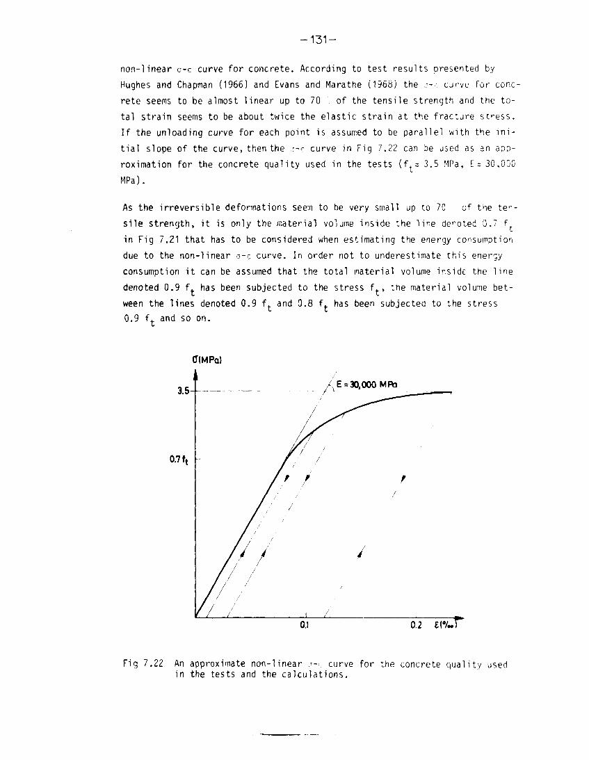
— 131 —

non-linear c-c curve for concrete. According to test results presented by

Hughes and Chapman (1966) and Evans and Marathe (1968) the J---. curve for conc-

rete seems to be almost linear up to 70 of the tensile strength and the to-

tal strain seems to be about twice the elastic strain at the fracture stress.

If the unloading curve for each point is assumed to be parallel with the ini-

tial slope of the curve, then the ~-c curve in Fig 7.22 can be used as an app-

roximation for the concrete quality used in the tests (ft= 3.5 MPa, E = 30,000

MPa).

As the irreversible deformations seem to be very small up to 70 of the ten-

sile strength, it is only the material volume inside the line denoted 0.7 f

in Fig 7.21 that has to be considered when estimating the energy consumption

due to the non-linear a-e curve. In order not to underestimate this energy

consumption it can be assumed that the total material volume inside the line

denoted 0.9 r has been subjected to the stress f t, the material volume bet-

ween the lines denoted 0.9 f. and 0.80.9 ft and so on.

has been subjected to the stress

d(MPa)

= 30,000MRa

0.7 ft

0.1 0.2

Fig 7.22 An approximate non-linear J-. curve for the concrete quality usedin the tests and the calculations.

-132-

On these assumptions the energy consumption due to the non-linearity of the

a-e curve is about 3.3 Nmm for the 50 mm deep beam and about 26 Nmm for the

200 mm deep beam, which means that the Gp value is overestimated by about 2.5

N/m for the low beam and by about 5 N/m for the deep beam (b=50 mm for both

the beams). These values are probably overestimations but yet they can be con-

sidered as small and it seems as though the effect of the energy consumption

due to the non-linearity of the a-c curve can normally be neglected. However,

as Gr is overestimated more for the deep beam than for the low beam, this

explains, at least to some extent, the small discrepancy between the Gp-va-

lues determined on beams of different depths.

As mentioned before the same relative loading velocity was used for both the

beam depths when Gp was determined by use of the three-point bend test. This

however means that the loading velocity in the fracture zone must be higher

for the 200 mm deep beam than for the 50 mm deep beam as the fracture zone

has to propagate a longer distance in the deeper beam. It has not been inves-

tigated how the loading velocity in the fracture zone affects the results but

it may cause a small size dependency of Gp. Furthermore, it is almost impossible

to obtain identical curing conditions for concrete specimens of different si-

zes. For example, the temperature always rises more in a large specimen than

in a small one during the curing period and this normally affects the develop-

ment of the material properties. This means that Gp can be slightly different

for different sizes of specimens, even if they are cured in the same environ-

ment. These effects can never be eliminated.

As can be seen there are many explanations to why Gp for concrete can be size

dependent. For this reason the very small variation of the Gp-values determined

by the use of quite different methods and different specimen geometries must be

accepted and Gp can be considered to be a useful material property for concrete.

7.4.5 Suitable specimen dimensions for the Gp test

There are many factors that must be considered when choosing suitable speci-

men dimensions for the Gp-test. These factors are listed and discussed below.

1. The capacity and dimensions of the testing machine limit the range

of possible specimen dimensions. It must also be possible to hand-

le the specimen during the test.

2. The fracture must bo stable. A suitable specimen geometry can be

chosen from the material properties, the stiffness of the testing

-133-

machine and Fig 7.9. Points 1 and 2 often greatly limit the [feasi-

bilities of choosing specimen geometry.

3. The energy consumption due to irreversible deformations ir. the spe-

cimen outside the fracture z o n e , which is discussed in 7.4.4, must

be minimized. To fulfil this the a/d-value should riot be too S":all.

The a/d-value ought to be equal to or larger than ".-.

4. The scatter ought to be minimized. G r is a mean value over fie <>'ea

through which the crack runs. This area decreases and the scatter

increases when the depth of the notch increases. For this rea"on,

a small a/d-value ought to be chosen. However, this opposes ;>n;rit

3. An a/d-value of 0.5 can be used as a compromise.

5. Energy consumption due to irreversible processes at the s u p n o r " ,

may occur. This is minimized if the beam is lonq and slender.

6. If the Gp-test is carried out on an uncompensated b o a - , set- 7.•'...:•,

it is then suitable if the fraction of energy supplied by the weight

of the beam is as small as possible, as this is less controlled than

the energy supplied by the testing machine. The fraction of ener-iy

supplied by the weight is minimized if the beam is small and the

ratio beam depth/beam length is large. This is contrary to point •"•.

The resistance to irreversible processes at the supports, tne spe-

cific gravity and the fracture mechanical properties of the matt-

rial will determine from case to case whether point b or point b

is the most important factor. (Point 6 should not be- < onside>-e": i*

compensated beams according to Fig 7.11 are u s e d ) .

7. The beam has to be representative of the material. Tne Jimension,

will then be determined by the largest irregularities in trie ma-

terial. A fair assumption is that the smallest dimensions of the

specimen ought to exceed the size of the largest irregularities

(aggregate p a r t i c l e s , p o r e s , etc) at least four times.

8. Another factor that has not been discussed so far is trie effect of

the radius of the crack tip. This ought to be as snail as D O S S i bio

and not exceed the dimensions of the irregularities in the material

All the points listed above cannot be fulfilled at the same time. One nas to

c o m p r o m i s e . H o w e v e r , point 2 must always be fulfilled, the fracture has to be

stable under any condition.

7.b Experimental^ ijivejsti^ajion o/_ the/ractuj^jnechanical properties ofconcrete '"

7.5.1 Testing procedure

Tests were performed in order to study three fundamental fr-icture mechanical

properties of concrete; the dynamic Young's rioduus ' L , , ) , t>>e fracture oners/

(Gp) and the tensile strength (f^). Besides these vrooerfies the flexural ten-

sile strength (f f) dnd the compression strength (f ) were also determined. -11

these properties can be determined on a single specimen, which is demonstra-

ted in a simple example in Fig 7.23.

1

1

2

3

U

5

MATERIAL PROPERTY

Dyn. Young's modulus

Fracture energy

Tensile strength

Flexural tensile strength

Compression strength

SPECIMEN

A1

L

I

1 ! ' 1

Fig 7.23 Test program for determining most of the fundamental mechanical pro-perties of concrete on a single specimen.

In the tests the program described in Fig 7.23 was used for determining all

the properties except the compression strength, which was determined on spe-

cimens with dimensions better fitted for available testing equipment. All the

tests were performed on wet specimens.

First the dynamic Young's modulus was determined by use of the method descri-

bed in 7.3, The specimen dimensions were 50 x 50 x 640 mm . After this a 4 mm

- 1 3 5 -

wide and 25 mm deep notch was sawn in the middle of the beam. The notched

beam was subjected to three-point bending in order to determine the frac-

ture energy and the test arrangement is presented in Fig 7.24. The distance

between the supports was chosen as 600 mm, which with the actual testing

machine (stiffness = 5,000 N/mm) always resulted in stable fractures, com-

pare Fig 7.9. As this test arrangement does not allow compensation for the

energy supplied by the weight of the beam, the evaluation method according

to (7:14) had to be used. For all the specimens the ligament was measured

after the test by use of vernier callipers. A typical load-deflection curve

for a Gr-test on concrete is shown in Fig 7.25.

During the Gr-test the beam was divided into two 32Ö pun long pieces. One of

these was used for determining the tensile strength by use of the :;ietnod pre-

sented in 7.2. The other piece was used for determining the flexural tensile

strenght by use of three-point bend tests where the distance between the sup-

ports was 200 mm. The supports used in these tests were the same as those

used in the Gp-tests, see Fig 7.24.

Finally the compression strength was determined on cubes with a side length

of 40 mm. The cubes were sawn out from beams with the dimensions 40 x 40 x3

160 mm and the load was applied to the sawn surfaces.

The five test methods are illustrated in Fig:s 7.26-7.30.

frP°i!t 25 mm

50mm

j-600 mm

Fig 7.24 Test arrangement used for the Gr-test.

-136-

0.2 04 0.6 0.8 1.0 b (mm)

Fig 7.25 A typical stable F-5 curve from the Gp-tests. The deformation in-cludes the deformations of the testing machine. The curve is rele-vant for mix 1 in Table 7:3 below.

Fig 7.26 Determination of the dynamic Young's modulus (E.J

-137-

Fig 7.27 Determination of the fracture energy (Gp),

Fig 7.28 Determination of the flexural tensile strength (f,)

-138-

Fiq 7.29 Determination of the ten- Fig 7.30 Determination of the compres-sile strength (f.). sion strength (f j.

7.5.2 Materials and mix proportions

Tne experiments were carried out in order to study the effect of the following

factors on the fracture mechanical properties of concrete; type of aggregate,

water-cement-ratio, volume fraction of cement paste, maximum aggregate partic-

le si^e and ane of concrete. The factors were varied one by one and the miring

proportions and the tosHna age:; for the concrete qualities that wore studied

are presented in Table 7:3. Ordinary Portland content was used. The same quali-

ty of aggregate 0-4 mm, nature material (not crushed) with a modulus of fine-

ness of 2.5, was used in all the mixtures and the content of aggregate 0-4 am;

was always 43 by volume of tne total aggregate content. When varying the

maximum aggregate particle size, aggregate >4 mm was composed according to

7:4.

As can be seen in Table 7:3,there are no differences between the mixtures 1

7, 10, 13 and 17. This concrete composition and age can be considered to be

a reference concrete quality.

-139-

Table 7:3 The mixtures and testing ages for the concretes used in thetests. The factor that was studied for each case is markedwith a circle. (Q=crushed quartzite, G=gravel (sea-bottommaterial), LS=crushed lime-stone, EC=expanded clay).

Mixture Type of !Water-Ce-aggrega- ment-P.atio Aggregatete >4 mmj (Vol)

Cement Paste Maximum Age of Cement-Particle concrete Sand (0-4)-Size (mm) (days^ Gravel(>4)-

Ratio (byweight)

1

2

3

4

5

6

7

9

10

11

12

13

14

15

16

17

18

Q

Q

Q

Q

0.5

0.5

0.5

0.5

0.5

0.5

0.5

0.5

0.5

0.5

0.5

0.5

0.5

0.5

0.5

0.5

0.5

0.5

0.5

0.5

0.5

0.5

0.5

0.5

0.5

12

12

12

12

12

12

12

12

28

28

23

28

28

28

28

28

1.0:2.04:2.71

1.0:2.04:2.77

1.0:2.04:2.64

1.0:2.04:0.72

1.0:1.55:2.05

1.0:1.80:2.38

1.0:2.04:2.71

1.0:2.55:3.38

28 1.0:2.60:3.44

28 1.0:2.04:2.71

28 1.0:1.68:2.23

28 1.0:2.04:2:71

28 1.0:2:04:2.71

28 1.0:2.04:2.71

1.0:2:04:2.71

1.0:2.04:2.71

1.0:2:04:2.71

1.0:2.04:2.71

Table 7:4 Composition of aggregate >4 mm.

Max particle ; Aggregate Aggregate Aggregatesize (mm) : 4-8 mm i 8-12 mm 12-16 mm

812

16

|ii

i 33

100 %50 L

1/3 I 33

-50

1/3 33 1/3

- 1 4 0 -

7.5.3 Preparation of specimens

For each concrete mixture 6 specimens (50 x 50 x 640 mm ) were cast on two

different occasions, i.e. a total of 12 specimens for each mixture. The spe-

cimens were stored in 100 % RH and +20°C during the first 24 h after casting

and then stored in lime saturated water (+20 C) until the time for testing.

After the E.-test the 25 mm deep notch was sawn by using a diamond saw. All

the tests were carried out on wet specimens. The compression strength was tes-

ted for each mixture on six specimens, which were sawn out from two beams.

7.5.4 Results

The results from the tests are presented in Table 7:5 and Fig:s 7.31-7.35.

In Table 7:5 90 ;i confidence intervals of the compression strength and the

flexural tensile strength are shown. The 90 ., confidence intervals of ft, Erf,

Gp and '. . are presented in F i g: s 7.31-7.35. When calculating the confidence

intervals of f. ., the mean values and the standard deviations of f., E, and

Gp were used.

7.5.5 Discussion

As can be seen in Fig 7.31, all the fracture mechanical parameters are great-

ly affected by the quality of the aggregate. The two stronger aggregates,

crushed quartzite and gravel, produce higher values of Gp than the two wea-

ker aggregates, crushed lime-stone and expanded clay. The explanation being

the difference of the crack propagation path. For the stronger materials,

especially for gravel, the crack runs around the aggregate particles, produ-

cing a large crack surface and a high value of Gp. For the weaker materials

the crack runs through the aggregate particles, consequently making the crack

surface and Gp small, see Fig 7.36. A strong aggregate material with a strong

bond probably also causes a more complex micro-crack formation in the paste

than a weak aggregate material with a poor bond. Naturally the fracture ener-

gy is also affected by the Gp-value of the aggregate, at least when the crack

passes through the aggregate particles, which explains the very low value for

the concrete containing expanded clay.

When a composite is subjected to load there will always be stress concentra-

tions in the material due to the difference between the Young's modulus of the

components. These stress concentrations decrease as the difference between the

Young's modulus of the components decrease. According to the test results it

seems as though the Young's modulus of the lime-stone is low and this is one

-141-

Tabie 7:5 The compression strength and the flexural tensile strength for theconcrete qualities used in the test. The figures represent 90confidence intervals.

Mixture

No.

1

2

3

4

5

6

7

8

9

10

11

12

13

14

15

16

17

18

Characteristic

1

Aggre-

gate

Water-

Cement-

Ratio

Vol. c em. p.Vol. aggr. y-

Max.

Particle

Size (mm)

Age of

Concrete

(days)

Parameter

CrushedQuarzite

Gravel agg.(Sea-bottom-mat.

CrushedLime-stone

Expanded Clay

0.3

0.4

0.5

0.7

0.4

0.5

0.6

8

12

16

2

7

28

91

Compr.Strength(MN/m2)40 mm cube

52.3-54.8

38.2-49.5

58.0-61.6

17.8-21.8

83.1-88.7

71.2-76.8

52.3-54.8

28.4-31.1

53.7-58.0

52.3-54.8

51.0-57.7

47.1-58.3

52.3-54.8

53.3-57.2

24.6-27.5

38.6-46.2

52.3-54.8

59.4-66.6

Flex. tens.StrenqthMN/m^"Beam deDth=50 mm

7.3-7.7

6.4-7.G

7.5-8.1

3.9-4.2

8.5-8.9

8.2-8.6

7.3-7.7

5.3-5.6

7.1-7.6

7.3-7.7

6.9-7.4

7.3-7.7

7.3-7.7

6.9-7.5

3.5-3.9

5.7-6.?

7.3-7.7

7.8-8.2

142-

f t(MPa)

Aggregate

Q G LS EC

Ed(MPa«103)

t50

25 -

1 1

1

1

Aggregate

Q G LS EC

G^N/m)

100

50

Aggregate

Q G LS EC

lc h(mm)

500

250I

Aggregate

Q G LS EC

Fig 7.31 Relations between the fracture mechanical properties and the quali-ty of aggregate. M=crushed quartzite, G=gravel, LS=crushed lime-stone, EC=expanded clay. (Mix 1-4).

- 1 4 - 3 -

ft(MPo)

3

2

I

Wo/C

0.3 0.5 0.7

Ed(MPa«i03)

50

25

ii

i

-

w0

1

/Ci ^

0.3 0.5 0.7

100ti

50

Wo/CL 1 I

0.3 0.5 0.7

lch(mm)

t500 -

250 II

wo/c03 0.5 0.7

Fig 7.32 Relations between the fracture mechanical properties of the con-crete and the water-cement-ratio.(Mix 5-8). W0/C=water-cement-ratio.

- 144 -

ft(MPa)

4

3

I I I

CP/A

(U 0.5 0.6

Ed(MPa»103)

50

25

CP/A

0.4 0.5 0.6

GF(N/m)

100

50

CP/A

0.4 0.5 0.6

lch(mm)

•500

250I I

CP/A

0.4 0.5 0.6

Fig 7.33 Relations between the fracture mechanical properties of the con-crete and the ratio volume cement paste/volume aggregate (CP/A),(Mix 9-11).

-145-

ft(MPa)

4

3

2

Max particlesize (mm)

8 12 16

E.fMPa-iö3)Q

50

25

i i

Max particlesize (mm)

i i

8 12 16

Gp(N/m)

100

50

Max particlesize (mm)

8 12 16

500

250

_ i i

Max particlesize (mm)

8 )2 16

Fig 7.34 Relations between the fracture mechanical properties of the con-crete and the maximum particle size of aggregate.(Mix 12-14).

-146-

(MPo)

Age (days)

2 7 28 91

•50

25

Agetdays).

2 7 28 91

GJN/m)F V

100 -

50

Age (days)

2 7 28 91

500

250

Age (days)

2 7 28 91

Fig 7.35 Relations between the fracture mechanical properties of the con-crete and the age of the concrete. (Mix 15-18).

- 1 4 7 -

Fig 7.36 In the gravel concrete (left) aggregate particles are extractedfrom the paste, while the fracture surface runs through the par-ticles in the lime-stone concrete (right).

explanation for the high tensile strength of the lime-stone concrete. Another

explanation is that the adhesion between the aggregate particles and the ce-

ment paste is probably better for the lime-stone than for the other types of

aggregate.

The low value of Gp for the lime-stone concrete together with the high value

of ff produces a low value of <. , . This material, and also the concrete con-

taining expanded clay, can therefore be considered as much more "brittle"

than the two concrete qualities containing crushed quartzite and gravel respec-

tively.

The tensile strength and the Young's modulus decrease, as expected, when the

water-cement-ratio increases, see Fig 7.32. Also Gr decreases when the water-

cement-ratio increases, at least when the water-cement-ratio exceeds 0.4. .ch

seems to be constant for water-cement-ratios up to 0.5 after which . , increa-

ses markedly. This implies that concrete with a high strength is more "britt-

le" than a concrete with low strength.

The tensile strength seems to be independent of the volume fraction of aggre-

gate, see Fig 7.33, while the Young's modulus naturally increases with increa-

sing aggregate content as the Young's modulus of the aggregate is higher than

the Young's modulus of the cement paste. Gp seems to increase somewhat with

an increasing volume fraction of aggregate. This can be explained by the fact

that the closer the aggregate particles are packed, the more complex the crack

propagation path is and the larger the crack surface and fracture energy be-

come. 5. . also increases somewhat with an increasing volume fraction of aggre-

gate. Gp and E, seem to be insensitive to the maximum aggregate particle size,

see Fig 7.34, while f. decreases and • . increases with increasing size of the

largest aggregate particles.

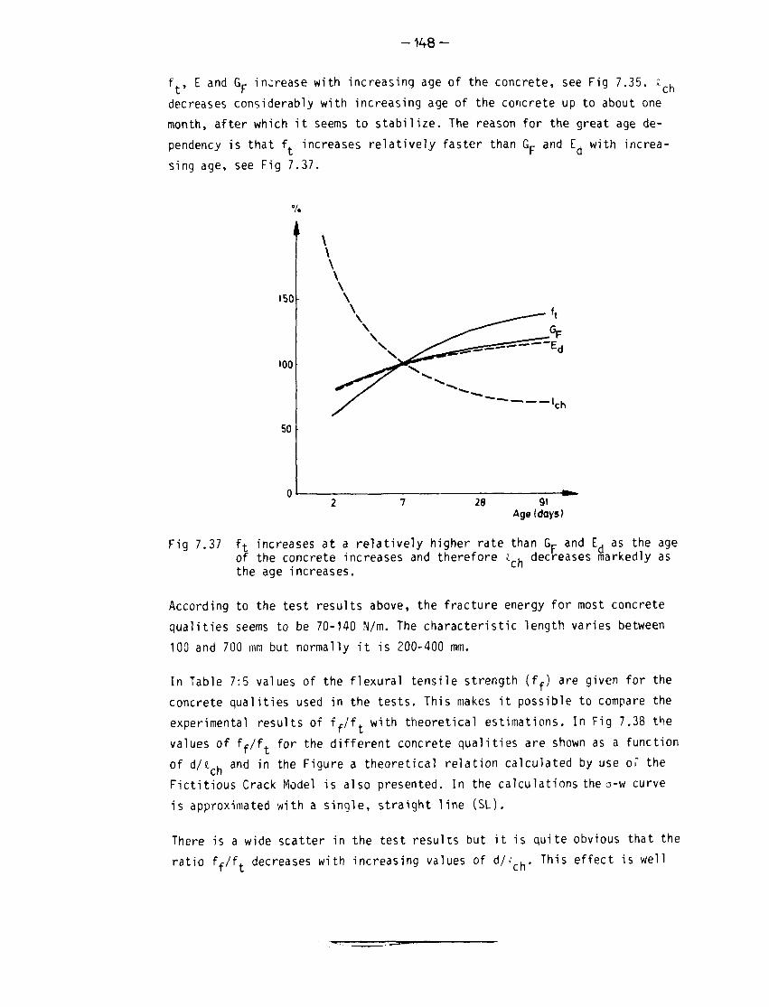
- 1 4 8 -

f., E and Gr increase with increasing age of the concrete, see Fig 7.35. z ,

decreases considerably with increasing age of the concrete up to about one

month, after which it seems to stabilize. The reason for the great age de-

pendency is that ft increases relatively faster than Gp and Erf with increa-

sing age, see Fig 7.37.

Fig 7.37

150

100

50

0

\\\\

[ \\

\\

\s.

Y

1 . .

" " " " 'ch

28 91Age (days)

ft increases at a relatively higher rate thanof the concrete increases and thereforethe age increases.

and Ed as the agei . decreases markedly as

According to the test results above, the fracture energy for most concrete

qualities seems to be 70-140 N/m. The characteristic length varies between

100 and 700 mm but normally it is 200-400 mm.

In Table 7:5 values of the flexural tensile strength (ff) are given for the

concrete qualities used in the tests. This makes it possible to compare the

experimental results of ff/f* with theoretical estimations. In Fig 7.38 the

values of f-r/f. for the different concrete qualities are shown as a function

of d/e h and in the Figure a theoretical relation calculated by use of the

Fictitious Crack Model is also presented. In the calculations the a-w curve

is approximated with a single, straight line (SL).

There is a wide scatter in the test results but it is quite obvious that the

ratio ff/ft decreases with increasing values of d/.'ch. This effect is well

- 1 4 9 -

ff/ft

1.5

•15

• 3

0.05 0.) 0.2 0.5d/lch

Fig 7.38 ff/f* as function of d/ich' The dots represent different concretequalities (the figures correspond to the mixtures defined inTable 7:3) and the curve represents a theoretical relation calcu-lated by means of the Fictitious Crack Model.

described by the theoretical curve in spite of the simplified assumptions (the

a-w curve is 'approximated to a straight line, the effect of the non-linearity

of the o-e curve is not considered and so on). This implies that the Ficti-

tious Crack Model, together with the material properties presented above, is

suitable for describing the fracture process for concrete.

- 1 5 1 -

DETERMINATION OF THE o-w CURVE FROM A STABLE TENSILE STRESS-DEFORMATIONCURVE

8.1 Introduction

As discussed in Chapter 3, the complete, stable tensile stress-deformation cur-

ve (o-5 curve) can be considered to consist of two parts; or\e part representing

the relation between stress and relative strain for the material outside the

fracture zone and one part representing the relation between stress and abso-

lute deformation of the fracture zone, see Fig 3.4. Fig 8.1 illustrates how

the a-e curve for the material outside the fracture zone and the :-w curve for

the fracture zone can be determined from a stable stress-deformation curve.

The fracture zone does not start developing until the tensile strength is rea-

ched and consequently c equals and w equals 0 for the stress -. on the

at 0=0,

e

w

Before*t

V lg0

Afterft

68 / lg

V6B

Fig 8.1 Determination of the o-c curve for the material outside the fracturezone and the o-w curve for the fracture zone from a stable tensilestress-deformation curve (o-s curve).

- 1 5 2 -

increasing part of the stress-deformation curve, o. and 6. are defined in Fig

8.1 and s,g is the gauge length for the deformation measurements. The stress

decreases when the fracture zone starts developing and consequently the mate-

rial outside the fracture zone becomes unloaded. In the Figure the unloading

curve for the material outside the fracture zone is assumed to be parallel

with the initial slope of the a-o curve. In real materials the unloading curve

may be slightly different due to creep effects for example. However, if the

gauge length for the deformation measurements is not too great, then a small

error in the slope of the unloading curve has a very little effect on the dis-

tance Sp-Sn in the Figure for all values of o., compare test results below.

A small fault in the slope of the unloading curve thus affects the c-w curve

very little and therefore the assumed slope ought to be useful. On the des-

cending part of the stress-deformation curve c then equals cR/f-q and w equals

6p-5n for the stress a..

Very few investigations regarding the stable stress-deformation curve (or stab-le stress-strain curve) for concrete are reported in literature. The reasonfor this is probably that it is necessary to use a very stiff tensile testingmachine in order to obtain a stable fracture and ordinary testing machines arenormally too weak, see 8.2.

Hughes and Chapman (1966) reported 5 individual stable stress-strain curves.

The tensile strengths of the concrete qualities tested ranged from 0.75 MPa

to 1.5 MPa, which is much lower than for a normal concrete quality.

Evans and Marathe (1968) reported 9 individual stress-strain curves for con-crete. The tensile strengths were also low in these tests, between 1.5 MPaand 3 MPa. The scatter between the individual curves was wide and for one con-crete quality they found a value of the strain at the tensile strength of 0.8°/oo, which seems quite unrealistic.

Heilmann, Hilsdorf and Finsterwalder (1969) carried out tensile tests on a

great number of concrete specimens. Most of their specimens failed in an un-

stable manner but they reported at least two individual stable stress-strain

curves. The tensile strength was less than 1.8 MPa for both the specimens,i.e.

lower than for a normal conrete quality.

It is easier to obtain a stable fracture for a material with a high value ofthe characteristic length (?

ru) than for a material with a low value, see 8.2,According to the results in 7'*>-4,s£ h seems to increase markedly with decrea-sing tensile strength and this is probably the reason why all the stable

- 1 5 3 -

stress-strain curves reported in the literature are relevant for concrete qua-

lities with very low values of the tensile strength (a low value of the ten-

sile strength may be due to shrinkage stresses).

In this Chapter a very stiff tensile testing machine of a new type is presen-

ted by which it is possible to follow the complete tensile stress-deformation

curve also for normal concrete qualities, o-w curves for a number of concrete

qualities ere presented as well.

8.2 Stability conditions for the direct tensile test

In Fig 8.2 a schematic illustration of a tensile test is shown. The testing ar-

rangement consists of a number of springs with different stiffnesses:

k. = the stiffness of the testing machine

kp = the stiffness of, for example, steel rods, which can be coupledparallel with the specimen in order to make the testing arrange-ment stiffer (cf Evans and Marathe, 1968).

k., = the stiffness of the specimen outside the fracture zone

F(w)

Fig 8.2 A schematic illustration of adirect tensile test, k., k~, k-,and k,(w) are the stiffnessesof the testing machine, of therods, which are coupled parallellwith the specimen, of the materialoutside the fracture zone and ofthe fracture zone respectively.

Fig 8.3 The system of springs usedfor the calculation of thestiffness (ks) of the tes-ting arrangement outsidethe fracture zone.

- 1 5 * * -

k.(w) = the stiffness of the fracture zone when the widening ofthe zone is w. This stiffness depends on the widening ofthe fracture zone according to the :-w curve for the mate-rial.

The amount of energy ((L) necessary to widen the fracture zone from 0 to w is:

w

QF = A [ j(w)dw (8:1)o

where A is the cross sectional area of the specimen at the position of the

fracture zone.

The amount of energy (Q ) stored in the system of springs outside the frac-

ture zone when the widening of the fracture zone is w can be expressed as

(compare (7:5)):

. A2(a(w))2 ,o.0.

where ks is the stiffness of the system of springs shown in Fig 8.3. The

springs with the stiffnesses k-| and k~ are parallel as they have to deform by

the same amount when the load F(w) is changed. This means that the stiffness

(k ) of the system of springs in Fig 8.3 is:

m r + IT

K2 1 3

(8:3)

If energy is consumed when the width of the fracture zone increases from w

to w + dw, then the fracture will be stable and this gives the condition of

stability for the direct tensile test (compare (7:6) and (7:7)):

k > - A 3o(w) (8:4)S ~3W~

If the unloading curve for the material outside the fracture zone is assumed

to be parallel with the initial slope of the curve (i.e. E) then the stiffness

for the specimen (with a constant cross sectional area) outside the fracture

zone is:

-155-

k3=TT (8:5)

where A is the cross sectional area of the specimen and i. is the specimen

length.

By use of (8:3), (8:4) and (8:5) the following expressions are derived:

1w

(8:6) is the stability condition when the widening of the fracture zone is w.

However, the fracture must be stable for all values of w and then the condi-

tion of stability becomes:

() h2v '•w'max

where (—) corresponds to the steepest slope of the ;-w curve.

If the G - W curve is approximated with a single straight line, then the slope

of curve is -f*./w , where wf is the maximum widening of the fracture zone,

where it is still able to transfer stress, see Fig 6.1. For the single line

approximation of the a-w curve w equals 2 Cr/f,. and thus the slope of the2curve can be expressed as -1/2 x fr/Gp. The single line approximation of the

a-w curve is the most favourable case and for other shapes of the --w curve

the steepest slope of the a-w curve can be expressed as -1/C x fs'Gr, where

C is a constant between 0 and 2 and C is dependent only on the shape of the

a-w curve. According to test results below the steepest slope of the --w curve

for concrete seems to be about twice the mean slope and then the value of C

becomes about 1 for this material.

The condition of stability for the direct tensile test can now, decor:) iny to

- 1 5 6 -

(8:7) and (4:15), be written as:

= c ' ch " Y^T ( 8 : 8 )

As can be seen from (8:8), the specimen length must be less than Zi . in order

to obtain a stable fracture, even if an infinitly stiff testing machine is

used. This means that the maximum length of the specimen for concrete is about

200-300 mm and for cement paste about 10-20 mm. However, these lengths are

considerably reduced when the weakness of the testing machine is considered,

which is illustrated in Fig 8.4. In the Figure the condition of stability ac-

cording to (8:8) is illustrated for different values of the cross sectional

area. The curves are relevant for e . - 250 mm, E = 40,000 MPa and C = 1, i.e.

a normal concrete quality. The horizontal axis in the Figure represents the

stiffness of the testing machine (k,) but of course this stiffness can be

replaced by k-, +ko> see (8:8), where k~ i3 the stiffness of the rods, which

can be coupled parallel with the specimen.

When carrying out tensile tests on concrete, all the specimen dimensions

ought to exceed the size of the maximum aggregate particles a few times. This

means that the smallest possible cross sectional area for a fine grained con-2

crete should be about 500 mm and for practical reasons the specimen length

ought to exceed at leas'- 40 mm. Even for these small specimen dimensions the

stiffness of the testing machine has to exceed about 100,000 N/mm in order

to obtain a stable fracture and the necessary stiffness increases rapidly

with increasing specimen dimensions.

Normally it is impossible to attach the specimen to the testing machine with-

out introducing weaknesses in the testing system. These weaknesses naturally

affect the stability and in reality the conditions of stability are therefore

harder than those given in (8:8) and Fig 8.4.

According to the results and the discussion above it seems quite obvious that

ordinary testing machines are too weak to be useful for stable tensile tests

on concrete. In order to obtain a stable fracture it is necessary to make the

testing machine stiffer by use of rods which are coupled parallel with the

specimen or to use special, very stiff testing machines. Such a testing ma-

chine, by which the complete tensile stress-deformation curve for concrete

can be determined, is described below.

-157-

Kmm)

50 -

Fig 8.4 Conditions of stability for the direct tensile test. The curves repre-sent the left limits of the areas of stability. The curves are rele-vant when irh is 250 mm, E=40,000 MPa and the constant C in (8:8) is 1.J.=specimen length, A=cross sectional area of the specimen and k.=thestiffness of the testing machine.

8.3 A stiff testing machine for stable tensile tests on concrete and _s_irnilarmaterials

In Fig 8.5 and Fig 8.6 a new type of tensile testing machine is shown by whichit is possible to carry out stable tensile tests on concrete specimens. Threealuminium columns U120 mm) are fixed between two concrete blocks and cylindri-cal heating elements are attached to the columns. The specimen is fixed (glued!in special holders between the concrete blocks. The aluminium columns expandwhen they are heated and then the specimen becomes subjected to load. The loadis registered by strain gauges, which are attached to one of the holders and

-158-

Fig 8.5 A stiff tensile testing machine for determination of the completestress-deformation curve. l=concrete block, 2=aluminium column,3=heating element, 4-strain gauges for load registration, 5=induc-tive deformation transducer for deformation registrations, 6=speci-men.

the deformations are registered by inductive deformation transducers, whichare fixed directly on the specimen. During the test the aluminium columns areinsulated with mineral wool in order to keep the temperature around the spe-cimen constant, see Fig 8.7.

Coils of tubes (inner diameter=4 mm) surround the aluminium columns and kero-

sene tempered by a thermostat can circulate in the tubes. This makes it pos-

sible to keep the temperature in the aluminium columns constant during the

time necessary (about 1 h) to obtain a sufficiently strong joint between the

specimen and the holders and to cool the column during the test and thereby

- 1 5 9 -

OJ

1/1c5o

5

5

> th

e <

.est

s

c

O3

ii n

e ra

'

3

QJ

OJ C

— cQJ O C

-C O =J4-J <_) i —

O

o o _QJ oo 3C i— • -o -i- L:

o •--• u E

QJ =3C O) —

•>- J C re-C *JO +-1

(T$ T ^ ^+—E C QJ

13 i—

C T3 OJ• r - OJ ^•»-J > +->oo OOJ E C+-J QJ O

0^ Ci— LO OJ•r- -r- OJL/1 L/lC LOQJ 4-> dJ+J C -O

QJ^ E C0>_ QJ (73• r - , (_)JJ QJLO l / l

cn OJQJ C -Q

oo

-160 —

Fig 8.8 The specimen between the holders in the stiff tensile testing machi-ne. The inductive deformation transducers are attached directly onthe specimen.

cause unloading of the specimen. The columns can also be cooled when a test

is finished , which greatly decreases the required time between two tests.

The thermal coefficient of expansion for aluminium is 24 x 10" K and thedeformation of the testing machine will be 1 mm if the temperature in the450 mm long aluminium columns is increased by 93 K. As the temperature of alu-minium can be raised to at least 200-300 C without losing its elastic beha-viour at low stresses, the deformation capacity of the testing machine is atleast 2 mm. This can be compared with the deformation capacity necessary tofollow the complete tensile stress-deformation curve for concrete, which isnormally less than 0.2 mm.

- 1 6 1 -

The maximum effect for the 6 heating elements (two on each column) is 2,200 W.

If all this energy was absorbed by the columns then the increase of the tem-

perature wou'ld be about 6 K/s (the density of aluminium is 2,700 kg/m and

the specific heat capacity is 880 Ws/kg K ) , which corresponds to about 38 ..m/

min. In reality some of the energy is lost and the deformation velocity for

the testing machine can be chosen,by varying the effect, between 0 and 30 ..m/

min. Of course the loading velocity can be increased if other heating ele-

ments are used.

In Fig 8.8 it is shown how the specimen is fixed between the supports by using

an adhesive (type Epoxy). The part of the holder closest to the specimen is

fixed to the other part of the holder by frictional forces caused by clamping

bolts. This means that the gap between the holders can bo adjusted, which is

necessary when attaching the specimen.

When the specimen is fixed in the testing machine by using an adhesive,it is

necessary to use a necked specimen, see 7.2. However, even if a necked speci-

men is used it is difficult to obtain a sufficiently strong joint if the speci-

men is wet. This problem is solved if the ends of the specimen are allowed to

dry in the air for a couple of hours before the time for the test, while all

the other surfaces are insulated by plastic foil. This method makes it possible

to keep the narrow section of the necked specimen wet and the end surfaces dry.

Before this drying process the ends of the specimen ought to be sandpapered

in order to remove the thin layer of weak cement paste, which always exists on

the surface of concrete.

8.4 Experimental determination of the g-w curve for concrete

8.4.1 Testing procedure

By use of the stiff tensile testing machine presented in 8.3, stable tensile

tests were carried out on a number of concrete qualities. In order to obtain

a stable fracture and to get a sufficiently strong joint between the specimen

and the holders in the testing machine, it is necessary to use small, necked

specimens. For this reason the specimen type denoted III in Fig 7.15 was used

in most tests. The deformations were measured on two opposite sides of the spe-

cimen by use of two inductive deformation transducers (gauge length 40 mm) and

the mean value was registered. The deformation velocity was about 20 ..m/min,

which means that the duration of each test was 5-10 minutes.

-162-

O(MPa)

necked specimensnotched specimens

10 20 30 40 50 60

Fig 8.9 0-w curves for necked and notched specimens respectively for theconcrete quality in Table 7*1 (28 days). The specimens correspondto type III and type IV in Kig 7.15.

The shape of the stress-deformation curve (o-6 curve) is naturally affected bythe geometry of the specimen. In order to study how the shape of the specimenaffects the a-w curve, stable tensile tests were carried out on necked andnotched specimens respectively, corresponding to the specimen types III andIV in Fig 7.15. The o-w curves were determined according to the method presen-ted in 8.1. These tests in fact are identical to the tensile tests presentedin 7.4.4 and Fig 7.18. The concrete quality used is presented in Table 7:1 andthe tests were performed when the concrete was 28 days old.

The results are presented in Fig 8.9 and it seems, even if the scatter is wide,as though there are no significant differences between the o-w curves represen-ting the two specimen geometries. The results in Fig 8.9 are in good agreementwith the fact that concrete is normally relatively notch insensitive when smallspecimens and small notch depths are concerned, see 6.2. This implies that thea-w curves are representative for the material, even if the curves are deter-mined on notched specimens.

- 163-

8.4.2 Materials and mix proporptions

Tests were carried out in order to study the effect of the water-cement-ratio,

the maximum aggregate particle size and the age of the concrete on the --w

curve. The four concrete qualities tested are presented in Table 8:1.

Table 8:1 The concrete qualities used in the tests.

Cement (ordinary Portland)

Water

Aggregate

Max aggr particle size

Age at the testing

Water-cement-ratio

kg/m3

kg/m3

kg/m3

mm

days

Mix 1

370

185

1755

8

28

0.5

Mix 2

296

207

1755

8

28

0.7

Mix 3

296

, 207

1755

2

28

i 0.7i

i Mix 4

37C

185

1755

7

! 0.5l

8.4.3 Preparation of specimens

For each concrete quality three specimens were cast in steel moulds. The speci-

mens were kept in lime saturated water (+20°) until one day before testing.

During the last day the ends of the specimens were allowed to dry while the

other surfaces were insulated by plastic foil. The olastic foil was not remo-

ved until the start of the test, i.e. the specimens were also insulated during

the time in the testing machine when the adhesive was hardening. The ends of

the specimens were sandpapered one day before the test.

8.4.3 Results and discussion

Fig 8.10 shows the three stress-deformation curves for the concrete quality

corresponding to mixture 4 in Table 8:1. When measuring the deformations a

40 mm effective gauge length was used. As can be seen in the Figure, the con-

crete is able to transfer stress even when it is considerably deformed and

the curves differ completely from a-6 curves for linear elastic materials. It

can also be observed that the descending parts of the curves are far from being

straight lines.

In Fig:s 8.11-8.13 o-6 curves for different concrete qualities are shown. Each

curve represents the mean value of three specimens. The values of the tensile

strength (ft) and the fracture energy (Gr) corresponding to these ;-• curves

are slightly higher than expected compared with the values in 7.5.4. However,

the composition of the concretes used for the stable tensile t.pst. is different

— 1 6 A - -

Ö(MPa)

I Gouge length- 60 mm

6 (/urn)

Fig 8.10 Stress-deformation curves for the concrete quality correspondingto mixture 4 in Table 8:1.

ö(MPa)

[Gouge length: 40 mm

0 100 60um)

Fig 8.11 Mean stress-deformation curves for concrete qualities with differentwater-cement ratios (mix 1 and mix 2 in Table 8:1).

- 165 —

Ö(MPa)

t3 1 1

w\ \\ • • • • .

\

\

Mix 2 max particle size = 8 mm

Mix 3 max particle size = 2 mm

Gauge length: 40 mrn|

50 100

Fig 8.12 Mean-stress-deformation curves for concrete qualities with differentmaximum aggregate particle sizes (mix 2 and mix 3 in Table 8:1).

CKMPa)

tMix 1 — — age 28 days

Mix i age 7 days

Gouge length: 40 mm|

50 100 6(/um)

Fig 8.13 Mean stress-deformation curves representing different ages of theconcrete (mix 1 and mix 4 respectively).

-166-

compared with the concretes used in 7.5. The tensile tests for each concrete

quality are only carried out on three specimens and this of course gives rise

to rather uncertain values of f. and Gp, which is another possible explana-

tion for the differences between the results from the two tests.

In Fig 8.11 curves representing concrete qualitieswitii different water-cement-

ratios are presented (mix 1 and mix 2 in Table 8:1). The curves differ in the

beginning but when the deformation exceeds 50 -m they become almost identical.

The curves in Fig 8.12 represent concrete qualities with different maximum par-

ticle sizes (mix 2 and mix 3 respectively). The main difference between the

curves is that the concrete with coarse aggregate seems to be able to transfer

stress at higher deformations than the concrete with fire aggregate. This in-

dicates that the stress transferring capability at high deformations is due

to frictional forces when the coarse aggregate particles are extracted from

the cement paste. These tests are carried out on concretes where the aggregate

particles have a higher strength than the cement paste and consequently the

aggregate particles are extracted from the cement paste when a crack propaga-

tes. For concretes where the strength of the cement paste is higher than the

strength of the aggregate (for example lime-stone concrete, light-weight con-

crete or high-strength concrete) the crack will pass through the aggregate par-

ticles and it is then probable that these materials will have a lower stress

transferring capability at high deformations than materials where the aggre-

gate particles are extracted from the cement-paste.

In Fig 8.13 curves representing different ages of the concrete are presented.

The effect of decreasing age on the a-6 curve seems to be similar to the effect

of increasing water-cement-ratio, compare Fig 8.11.

In order to describe the properties of the fracture zone it is not the a-5 cur-

ves but the c-w curves that are of interest. In Fig 8.14 the J-W curves for

the four concrete qualities used in the test are presented.

In Fig 8.15 the a-w curves are shown in an alternative way; o and w on the axes

in Fig 8.14 are replaced by o/f. and w/w , i.e. Fig 8.15 shows the shape func-

tions (h(w/w )) of the curves according to (4:14/. In the Figure a a-w curve

approximated with two straight lines is also presented and this curve is iden-

tical to the a-w curve (C) in Fig 6.3. For this approximation of the a-w curve

w is 3.6 Gp/ft and this expression for w has also been used for the real

a-w curves. As can be seen in the Figure, the shapes of the a-w curves for the

four different concrete qualities are about the same and the two-line approxi-

-167-

ö(MPa)

mix 1mix 2mix 3mix A

50

Fig 8.14 a-w curves for the four concrete qualities presented in Table 8:

1/3

mix 1mix 2

— mix 3— mixA

0.5 10 w/wc

Fig 8.15 o/f+ as function of w/w for the four concrete qualities presentedin Table 8:1. The a-w curve approximated with two straight linescorresponds to the curve in Fig 6.3.

-168-

mation of the a-w curve shown in the Figure seems suitable for these concrete

qua!ities.

For all the concrete qualities used in the test the aggregate particles are

extracted from the cement-paste at crack propagation. The shape of the c-w

curve may be different if the crack passes through the aggregate particles.

However, the shape of the a-w curves shown in Fig 8.15 ought to be realistic

for most concrete qualities and this means that the o-w curve can be deter-

mined when the tensile strength (ft) and the fracture energy (Gp) are known,

see 4.5. A consequence of this is that no "complicated" stable tensile tests

have to be carried out in order to determine the J-W curve for concrete but

the curve can be determined by use of the "simple" f^- and Gr-tests presen-

ted in Chapter 7.

In Fig 8.16 load-deflection curves for a notched beam subjected to three-point

bending are shown. The unbroken lines represent experimental results from the

F(N)

800

600

exp.theor.(C)theor.(SL)

GF-137N/m

b-005mft- 3.33 MPG

G -115 N/m

Fig 8.16 Experimental and theoretical load-deflection curves for three-pointbend tests on notched beams. In the calculation; the o-w curve wasapproximated according to Fig 6.1 (SL) and Fig ij.3 (C) respectively.

-169-

tests on the 200 mm deep beams presented in 7.4.4 and Fig 7.18. In the testssix beams were tested in order to determine the fracture energy and the twoexperimental curves in Fig 8.16 correspond to the two beams, which producedthe highest and the lowest value of the fracture energy respectively. The theo-retical curves, calculated by means of the Fictitious Crack Model, correspondto two different approximations of the o-w curve; the single line approxima-tion (SL) according to Fig 6.1 and the two line approximation (C) accordingto Fig 6.3 (which is identical to the approximation in Fig 8.15) respective-ly. The mean value of Gr- for the concrete quality is about 124 N/m (see testresults in Fig 7.18) and ft is about 3.33 MPa (see results in Fig 8.9, whichare relevant for this concrete quality). These values were used in the calcula-tions and the Young's modulus was assumed to be 3G,000 MPa. As can be seen inthe Figure the theoretical curve according to the two-line approximation ofthe o-w curve is in good agreement with the experimental curves. Togetherwith calculation results presented in Chapter 6 this implies that the shapeof the o-w curve presented in Fig 6.3 and Fig 8.15 is suitable for r.ormal con-crete qualities.

-171 -

9 REFERENCES

Andersson, H. and H. Bergkvist (1970). Analysis of a non-linear crack model.J. Meoh. Phys. Solids, Vol 18, pp. 1-28.

Barenblatt, G.J. (1962). The mathematical theory of equilibrium crack in thebrittle fracture. Advance in Applied Mechanics, Vol 7, pp. 55-125.

Bastgen, K.J. and V. Hermann (1977). Experience made in determining the staticmodulus of elasticity of concrete. Matc»iaux et Ccnctrud::n.-, Vol 10, pp.357-364.

Ba2ant, Z.P. and L. Cedolin (1979). Blunt crack band propagation in finiteelement analysis. -/. of Engineer'na :'er'Jun'e.- ::\':V:\":, Vol 105, No EM 2,pp. 297-315.

Brown, J.H. (1972). Measuring the fracture toughness of cement paste and mor-tar. Magazine of Concrete Revsaven, Vol 24, pp. 185-196.

Brown, J.H. and C D . Pomeroy (1973). Fracture toughness of cement paste andmortars. Ce-:. and Conor, kes., Vol 3, pp. 475-480.

Brown, W.F. and J.E. Srawley (1967). rian-- r^vi'>: r>' -:- ;>< > \. .••• ;..••••..• •'High Strength Metall',? Material?. ASTM-STP 410.

Carlsson, J. (1976). Fracture 'A * Ayr: i o . Ingenjörsförlaget, Katrineholm,Sweden (in Swedish).

Carpinteri, A. (1981). Experimental determination of fracture toughness para-meters K j C and Jjr, for aggregative materials. A I-m'.•..- '-; /•>:>• ...•-• .-, .•-••..5th International Conference on Fracture, Cannes 29 March-2 April, 1981. pp.1491-1498. Ed. D. Francois, Pergamon Press.

Chhuy, S., M. E. Benkirane, J. Baron and D. Francois (1981). Crack propaga-tion in prestressed concrete. Interaction with concrete. •;.••;•>.'..• '• •'.'-,.••Research. 5th International Conference on Fracture, Cannes 29 March-2 April,1981. pp. 1507-1514. Ed. D. Francois, Pergamon Press.

Cooper, G.A. (1977). Optimization of the three-point bend test for fractureenergy measurement. J. cf Mate-rialr, Co'- :n:v!, Vol 12, pp. 277-289.

Dugdale, D.S. (1960). Yielding of steel sheets containing slits. -'. •'::. -•..Phys. Col ide, Vol 8, pp. 100-104.

Entov, V.M. and V.T. Yagust (1975). Experimental investigation of laws gover-ning quasi-static development of macrocracks in concrete. ;:• "'/•./-.• v '•'•.-,Vol 10, pp. 87-95.

Evans, R.H. and M.S. Marathe (1968). Microcrackning and stress-strain curvesfor concrete in tension. Materiaux ,-.t :onr.t.ru-t ':.->:.>, No 1. pp. 61-64.

GjjJrv, D.E., S.I. Stfrensen and A. Arnesen (1977). Notch sensitivity and frac-ture toughness of concrete. <:.-•>-,. and C;_,n.*v. •••.:., Vol 7, pp. 333-344.

Griffith, A.A. (1921). The phenomena of rupture and flow in solids. .• ''.Trana. Rou. Coc, series A221, pp. 163-198.

-172-

Gustafsson, P.J. (1977). Fracture Mechanics Applied to Lightweight Concreteand Fibre-reinforced Concrete. Report TVBM-5001, Division of Building Mate-rials, University of Lund, Sweden (in Swedish)

Halvorser, G.T. (1980). J-integral study of steel fibre reinforced concrete.The Int. J. of Cement Composites, Vol 2, pp. 13-22.

Harris, B., J. Varlow and C D . Ellis (1972). The fracture behaviour of fibrereinforced concrete. Cem. and Conor. Res., Vol 2, pp. 447-461.

Heilnwnn, H.G., H.H. Hilsdorf and K. Finsterwalder (1969). Festigkeit undVerfcrmung von Beton unter Zugspannungen. Dcutscher Ausschuss fiir Stahl-beton, Heft 203, W. Ernst& Sohn, Berlin (in German).

Hernelind, J. and L.G. Pärletun (1974). EUFEMI (manual for FEM-calculations).Div. of Solid Mechanics, Lund Institute of Technology, Sweden (in Swedish).

Higgins, D.D. and J.E. Bailey (1976). Fracture measurements on cement paste.J. of Materials Science, Vol 11, pp. 1995-2003.

Hiliemeier, B. and H.K. Hilsdorf (1977). Fracture mechanics studies on con-crete compounds. Cem. and Conor. Res. Vol 7, pp. 523-536.

Hillerborg, A., M. Modéer and P.£. Petersson (1976). Analysis of crack forma-tion and crack growth in concrete by means of fracture mechanics and finiteelements. Cem. and Conor. Res., Vol 6, pp. 773-782.

Hillerborg et al (1977). Compendium in Building Materials AK. Lund Instituteof Technology, Division of Building Materials, Lund, Sweden (in Swedish).

Hillerborg, A. (1980). Analysis of fracture by means of the fictitious crackmodel, particulary for fibre reinforced concrete. Int. J. of Cement Composi-tes, Vol 2, pp. 177-184.

Hillerborg, A. and P.E. Petersson (1981). Fracture mechanical calculations,test methods and results for concrete and similar materials. AdJanies inFracture Research. 5th International Conference on Fracture, Cannes 29 March-2 April, 1981. pp. 1515-1522. Ed. D. Francois, Pergamon Press.

Hughes, B.P. and G.P. Chapman (1965). Direct tensile test for concrete usingmodern adhesives. Bulletin P.I.IEM, No 26, pp. 77-80.

Hughes, B.P. and G.P. Chapman (1966). The complete stress-strain curve forconcrete in direct tension, bulletin RILEM, NO 30, pp. 95-97.

Janson, J. and J. Hult (1977). Fracture mechanics and damage mechanics, acombined approach. J. de Me'canique Appliquec,Vo] 1, pp. 69-84.

Janson, J. (1978). Damage model for crack growth and instability. Eng. Frac-ture Mechanics, Vol 10, pp. 795-806.

Johnston, C D . and E.H. Sidwell (1968). Testing concrete in tension and incompression. Mag. of Cone. Res., Vol 20, pp. 221-228.

Kachanov, L.M. (1958). Time of the rupture process under creep conditions.Izo. Akad. Muk SSCF, Otd. Tekh. Nauk, Vol 8, pp. 26-31.

Kadlecek, V. and Z. Spetla (1965). Effect of size and shape of test specimenson the direct tensile strength of concrete. Bulletin 1ULEM, No 36, pp. 175-184.

- 1 7 3 -

Kaplan, M.F. (1961). Crack propagation and the fracture of concrete. J. ofthe American Concrete Institute, Vol 58, pp. 591-609.

Knott, J.F. (1979). Fundamental of Fracture Mechanics. 3rd edition, Butter-worths, London.

Mai, Y.W. (1979).Strength and fracture properties of asbestos-cement mortarcomposites. J. of Materials Science, Vol 14, pp. 2091-2102.

Mai, Y.W., R.M.L. Foote and B. Cotterell (1980). Size effects and scalinglaws of fracture in asbestos cement. The Int. J. of Cement Conr-ocitej, Vol 2,pp. 23-34.

Mayer, H. (1967). Die Berechnung von Durchbiegung von Stahlbetonbauteilen.Deutcher Ausschuss fur Stahlbeton. W. Ernst & Sohn, Berlin (in German).

Mazars, J. (1981). Mechanical damage and fracture of concrete structures.Advances in Fracture Research. 5th International Conference on Fracture,Cannes 29 March-2 April, 1981. pp. 1499-1506. Ed. D. Francois, Pergamon Press.

Mindess, S. and J.S. Nadeau (1976). Effect of notch width on K.- for mortarand concrete. Cem. and Concr. Res., Vol 6, pp. 529-534.

Mindess, S., F.V. Lawrence and C.E. Kesler (1977). The J-integral as a frac-ture criterion for fibre reinforced concrete. Cem. and Conor. Fes., Voi 7,pp. 731-742.

Mindess, S. and S. Diamond (1980). A preliminary SEM study of crack propa-gation in mortar. Cem. and Concr. Res., Vol 10, pp. 509-519.

Moavenzadeh, F. ana R. Kuguel (1969). Fracture of concrete. J. of Materials,Vol 4, pp. 497-519.

Modéer, M. (1979). A Fracture Mechanics Approach to Failure Analyses of Con-crete Materials. Report TVBM-1001, Division of Building Materials, Universityof Lund, Sweden.

Nadeau, J.S, S. Mindess and J.M. Hay (1974). Slow crack growth in cementpaste. J. of the American Ceramic 'Joe, Vol 57, pp. 51-54.

Naus, D. and J. Lott (1968). Fracture Toughness of Portland Cerent Concr,: t s.Report No 314, Dep. of Theoretical and Applied Mechanics, University of 111.,Urbana, 111.

Naus, D.J. and J.L. Lott (1969). Fracture toughness of portland cement con-cretes. J. of the American Concr. Inst., Vol 66, pp. 481-489.

Ohigashi, T (1978). Measurement of effective fracture energy of glass fibrereinforced cement. Testing and Test Methods of Fibre Cerr.cnt-Cr^'O,;:','.v.RILEM Symposium, 5th-7th April 1978, Ed. R.N.'Swamy, pp. 67-78.'

Petersson, P.E. (1980a). Fracture mechanical calculations and tests for fibrereinforced cementitious materials. Advances in Cement-matrix ('^"-posites.Proceedings, Symposium L, Materials Research Society, Annual meeting, BostonNovember 17-18, 1980, pp. 95-106.

Petersson, P.E. (1980b). Fracture energy of concrete: Method of determination.Cem. and Concr. Res., Vol 10, pp. 78-89.

Petersson, P.E. (1980c), Fracture energy of concrete: Practical performanceand experimental results. Cen. and Conor. Res., Vol 10, Dp. 91-101.

Petersson, P.E. and P.J. Gustafsson (1980). A model for calculation of crackgrowth in concrete-like materials, 'lunerical Methclc in Fracture Mer>nar.:os,pp. 707-719. Pineridge Press, Swansen, U.K.

Peterssc.i, P.E. (1981). Direct tensile tests on prismatic concrete specimens.Cen. and C oner. Res., Vol 11, pp. 51-56.

Pfeiffer, G. (1968). Eereohnung und harnessw.g ;-:n i--indarf'g-:n Träg.rr\. Werner-Verlag, Dusseldorf (in German).

Rice, J.R. (1968). Path independent integral and approximate analysis ofstrain concentration by notches and cracks. J. of Ar-rlied Meohanios, Trans-actions, ASME, Vol 35, pp. 379-386.

Rice, J.R., P.C. Paris and J.G. Merkle (1973). Some further results of J-in-tegral analysis and estimates, ihwecs in Flo:: 'irovtk -mi Fracture COWVIK^SSTesting, ASTM STP 536, pp. 231-245".

Sabnis, G.M. and S.M. Mirza (1979). Size effects in model concretes? ,\ cfStruct. Dii\, A'JCE, Vol 105, pp. 1007-1020.

Shah, S.P. and F.J. Me Garry (1971). Griffith fracture criterion and concrete.J. of the Engineering Mechanics Division, December 1971, pp. 1663-1676.

Sok, C (1978). Etude de la propagation d'un fissure dans un béton non armé.Bull. Liaison Labo. P. et Ch. , Vol 98, pp. 73-84 (in French).

Sok, C , J. Baron and D. Francois (1979). Mecanique de la rupture appliqueeau beton hydralique. Cem. and Conor. Res., Vol 9, pp. 641-648 (in French).

Strange, P.C. and A.H. Bryant (1979). The role of aggregate in the fractureof concrete. J. of Materials Science, Vol 14, pp. 1863-1868.

Velazco, G., K. Visalvanich and S.P. Shah (1980). Fracture behaviour and ana-lysis of fibre reinforced concrete beams. Cem. and Conor. Res., Vol 10, pp.41-51.

Vinkeloe, R. (1962). Prlifverfahren zur ermittlung des dynamischen Elastizi-tätsmodulus von Betonprismen. Tonindustris Zeitung, Vol 86, pp. 272-276(in German).

Walsh, P.F. (1972). Fracture of plain concrete. Indian Conor. Journal, Vol46, pp. 469-476.

Wecharatana, M. and S.P. Shah (1980). Double torsion tests for studying slowcrack growth of Portland cement mortar. Cem. and Conor. Res,., Vol 10, pp.833-844.

Welch, G.3. and B. Haisman (1969). The application of fracture mechanics toconcrete and the measurement of fracture toughness. Materiaux et Construc-tions, Vol 2,pp. 171-177.

Wright, P.J.F. (1952). The effect of the method of test on the flexuralstrength of concrete. Mag. of Conor. Res., Vol 4, pp 67-76.

Ziegeldorf, S., H.S. Muller and H.K. Hilsdorf (1980). A model law for the notchsensitivity of brittle materials. Cem. and Conor. Res., Vol 10, pp. 589-C99.