Corporate Bond Valuation and Hedging with Stochastic...

Corporate Bond Valuation and Hedging with Stochastic Interest Rates

and Endogenous Bankruptcy

Viral V. Acharya London Business School

Jennifer N. Carpenter New York University

This paper analyzes corporate bond valuation and optimal call and default rules when

interest rates and firm value are stochastic. It then uses the results to explain the dynamics of hedging. Bankruptcy rules are important determinants of corporate bond sensitivity to

interest rates and firm value. Although endogenous and exogenous bankruptcy models

can be calibrated to produce the same prices, they can have very different hedging

implications. We show that empirical results on the relation between corporate spreads and Treasury rates provide evidence on duration, and we find that the endogenous model

explains the empirical patterns better than do typical exogenous models.

Corporate bonds are standard investment instruments, yet the embedded options they contain are quite complex. Most corporate bonds are callable and

call provisions interact with default risk. In any case, corporate bond investors

face the problem of managing interest rate and credit risk simultaneously. This paper examines the valuation and risk management of callable default-

able bonds when both interest rates and firm value are stochastic and when

the issuer follows optimal call and default rules. To our knowledge, this is the

first model of coupon-bearing corporate debt that incorporates both stochastic

interest rates and endogenous bankruptcy. Existing models either treat interest

rates as constant or impose exogenous default rules. These assumptions can

significantly impact bond pricing and hedging. Yield spreads can be sensitive

to interest rate levels, volatility, and correlation with firm value. Spreads are

also sensitive to assumptions about the bankruptcy process. Some exogenous

bankruptcy specifications produce negative spreads. Even when they guarantee positive spreads, exogenous default models can have hedging implications that are very different from those of endogenous default models.

Working with a general Markov interest rate process, we develop analytical results about the existence and shape of optimal call and default boundaries.

We would like to thank Edward Altman, Yakov Amihud, Alexander Butler, Darrell Duffie, Edwin Elton,

Stephen Figlewski, Michael Fishman, Kenneth Garbade, Jing-zhi Huang, Kose John, Krishna Ramaswamy, Marti Subrahmanyam, Rangarajan Sundaram, Stuart Turbull, Luigi Zingales, and two anonymous referees for helpful comments and suggestions. Address correspondence to Jennifer N. Carpenter, Stem School of Business, New York University, 44 W. 4th Street, Suite 9-190, New York, NY 10012, or e-mail:

[email protected].

The Review of Financial Studies Winter 2002 Vol. 15, No. 5, pp. 1355-1383 ? 2002 The Society for Financial Studies

The Review of Financial Studies / v 15 n 5 2002

Then we numerically study the dynamics of hedging, using the results on

exercise boundaries to explain patterns in bond duration and sensitivity to firm value. Finally, we link duration to the slope coefficient in a regression of changes in yield spreads on changes in interest rates and find that the

endogenous bankruptcy model seems to explain empirical patterns in the

spread-rate relation better than typical exogenous bankruptcy models.

To clarify the interaction between call provisions and default risk, we

model the callable defaultable bond together with its pure callable and pure defaultable counterparts. We view each of the three bonds as a host bond

minus a call option on that host bond. The call options differ only in their

strike prices. The strike of the pure call is the provisional call price. The

strike of pure default option is firm value. The strike of the option to call or

default is the minimum of the two.

Treating defaultables like callables illuminates their similarities and dif-

ferences. For example, spreads on all bonds, not just callables, narrow with

interest rates because all embedded option values decline with the value of

the underlying host bond. On the other hand, credit spreads can increase or

decrease with interest rate risk, depending on how interest rates correlate

with firm value.

The paper provides a number of analytical results. With regard to valuation, we prove that all three bond prices are increasing in the host bond price, but

at rates less than one. The corporate bond prices are also increasing in firm

value, at rates less than one. With regard to optimal call and default rules, we establish the existence and shape of optimal exercise boundaries. Like

the optimal exercise policy for the pure callable, the optimal policies for

corporate bonds are defined by a critical host bond price above which the

bond issuer either calls or defaults and below which he continues to service

the debt. In the case of the corporate bonds, this critical host bond price is a

function of firm value, forming an upward-sloping boundary for noncallables

and a hump-shaped boundary for callables.

We also compare the different boundaries, showing how the call and

default options embedded in the callable defaultable bond interact on its

optimal exercise policy. The default region of the callable defaultable bond

is smaller than that of the pure defaultable and its call region is smaller than

that of the pure callable. When both options are present, the value of pre-

serving one option can make it optimal for the issuer to continue servicing the debt when it would otherwise exercise the other option.

We then numerically study the dynamics of hedging. Since duration is high when call and default are remote, the exercise boundaries explain a variety of patterns in duration. First, all bond durations are decreasing in the host

bond price as increases in the host bond price bring the bonds closer to the

exercise boundary. Second, as functions of firm value, bond durations inherit

the shape of the boundaries, because the boundary quantifies how far away the bond is from call or default. Thus, the duration of the pure defaultable

1356

Corporate Bond Valuation

bond is increasing in firm value, while the duration of the callable defaultable

bond is hump-shaped. In addition, the call and default options interact on

duration. A call provision by itself reduces duration, as does default risk by itself. However, a call provision can increase the duration of a defaultable

bond and default risk can increase the duration of a callable bond because

the presence of one option delays the exercise of the other.

Next, we draw a link between duration and the slope coefficient in the

regressions of changes in corporate yield spreads on changes in Treasury bond rates performed by Duffee (1998). The variation in this slope coefficient

across bond rating gives evidence on the empirical relation between dura-

tion and firm value. In Duffee's study, these slope coefficients are increasing in bond rating for noncallable bonds and hump-shaped in bond rating for

callable bonds, like the duration-firm value functions implied by our model.

By contrast, in a model with exogenous default rules, as typically specified in the literature, duration is a U-shaped function of firm value near default.

Finally, we illustrate the dynamics of bond sensitivity to firm value. Sen-

sitivity to firm value is high when default is near and low when call is near.

This explains three effects. First, the pure defaultable bond's sensitivity to

firm value is increasing in the host bond price, as increases in the host bond

price bring the bond closer to default. Second, both the callable default-

able and the pure defaultable bond sensitivity to firm value decrease in firm

value as default becomes remote. Third, the sensitivity of the callable default-

able bond is uniformly lower than that of the noncallable because default is

always farther away. This last effect suggests that a call provision mitigates the underinvestment problem of levered equity described by Myers (1977).

The paper proceeds as follows. Section 1 summarizes the related litera-

ture. Section 2 describes the financial market and the bonds with embedded

options and gives analytical results on valuation and numerical results on

yield spreads. Section 3 contains analytical results on optimal call and default

policies. Section 4 studies corporate bond risk management. Section 5 con-

cludes.

1. Related Literature

Much of the existing theory of defaultable debt treats interest rates as con-

stant in order to focus on the problems of optimal or strategic behavior of

competing corporate claimants. Merton (1974) analyzes a risky zero-coupon bond and characterizes the optimal call policy for a callable coupon bond.

Brennan and Schwartz (1977a) model callable convertible debt. Black and

Cox (1976) and Geske (1977) value coupon-paying debt when asset sales are

restricted and solve for the equity holders' optimal default policy. Fischer,

Heinkel, and Zechner (1989a,b), Leland (1994), Leland and Toft (1996), Leland (1998), and Goldstein, Ju, and Leland (2000) embed the optimal default policy, and in some cases, the optimal call policy, in the problem of

1357


optimal capital structure. Models such as Anderson and Sundaresan (1996),

Huang (1997), Mella-Barral and Perraudin (1997), Acharya et al. (2002), and

Fan and Sundaresan (2000) introduce costly liquidations and treat bankruptcy as a bargaining game.

Other models allow for stochastic interest rates and take a different approach to the treatment of bankruptcy. Some impose exogenous bankruptcy trig-

gers in the form of critical asset values or payout levels. These include the

models of Brennan and Schwartz (1980), Kim, Ramaswamy, and Sundaresan

(1993), Nielsen, Saa-Requejo, and Santa-Clara (1993), Longstaff and Schwa-

rtz (1995), Brys and de Varenne (1997), and Collin-Dufresne and Goldstein

(2001). Cooper and Mello (1991) and Abken (1993) model defaultable swaps

assuming that equity holders can sell assets to make swap or bond payments. Shimko, Tejima, and Van Deventer (1993) model a zero-coupon bond.

Other papers model default risk with a hazard rate or stochastic credit spread.

See, for example, Ramaswamy and Sundaresan (1986), Jarrow, Lando, and

Turnbull (1993), Madan and Unal (1993), Jarrow and Turnbull (1995), Duffie

and Huang (1996), Duffie and Singleton (1999), Das and Sundaram (2000), and Acharya, Das, and Sundaram (2002).

Another related literature analyzes callable bonds with stochastic interest

rates in the absence of default risk. This includes Brennan and Schwartz

(1977b) and Courtadon (1982). Related work on American options on nonde-

faultable bonds includes Ho, Stapleton, and Subrahmanyam (1997), Jorgensen

(1997), and Peterson, Stapleton, and Subrahmanyam (1998). Amin and Jarrow

(1992) provide a general analysis of American options on risky assets in the

presence of stochastic interest rates.

2. Valuation

This section first describes the financial market and corporate setting formally and develops a framework which treats all issuer options as call options on

an underlying host bond. Then we present analytical results about bond and

option values and illustrate some implications for yield spreads.

2.1 Interest rate and firm value specifications

Suppose investors can trade continuously in a complete, frictionless, arbitrage- free financial market. There exists an equivalent martingale measure 2? under

which the expected rate of return on all assets at time t is equal to the interest

rate r,. The interest rate is a nonnegative one-factor diffusion described by the equation

drt = /,(rt, t) dt + a(r, t) dZt, (1)

1358


where Z is a Brownian motion under 2 and ,u and o' are continuous and

satisfy Lipschitz and linear growth conditions. That is, for some constant L,

,t and o satisfy

I\(x, t) -u(y, t)l + la(x, t) - (y, t)l < Llx- yl, (2)

I/(x, t)j + o(x, t)l < L(1 + I xl) (3)

for all x, y, t E +.

Next, consider a firm with a single bond outstanding. The bond has a fixed

continuous coupon c and maturity T. Without loss of generality, suppose the

par value of the bond is one, and all other values are in multiples of this par value. The value of the firm is equal to the value of its assets, V, independent of its capital structure. Firm value evolves according to the equation

d = (rt - t)dt + tdW, (4) V

where W is a Brownian motion under P with d(W, Z)t = Pt dt and Yt > 0,

(t > 0, and Pt E (-1, 1) are deterministic functions of time. Protective bond

covenants prevent equity holders from altering the firm's payout rate y or

volatility 4.

2.2 Option and bond valuation

We consider the case that the firm's bond is callable with a call price schedule

kt. To clarify the interaction between the call provision and default risk, we also model the pure defaultable version and the pure callable version.

The pure defaultable is the noncallable bond with same coupon, maturity, and issuer. The pure callable is the nondefaultable bond with same coupon,

maturity, and call provision. The pure callable bond is equivalent to a noncallable, nondefaultable host

bond with the same coupon and maturity minus a call option on that host

bond with strike price equal to the provisional call price. Letting Pt denote

the price of the host bond, the payoff of exercising the option at time t is

P- kt. We assume that kt lies below the supremum of Pt for all t e [0, T), so that the option is always nontrivial.

The pure defaultable bond can also be viewed as a host bond minus a

call option on that host bond, but the strike price is equal to firm value Vt. The firm's owners are long the firm assets, short the host bond, and long an

option to default. This option to default, or buy back the bond in exchange for the firm, is a kind of call on the host bond. Its exercise value is P - Vt.

When the bond is both callable and defaultable, it is again equivalent to a

host bond minus a call option on that host bond. In this case the strike price is equal to the minimum of the provisional call price and firm value, kt A Vt. The issuer is long the firm, short the host bond, and long the option to stop

1359


servicing the debt, i.e., buy back the host bond, either by calling and paying

kt or by giving up the firm worth V,. The exercise value of this option to

stop servicing the debt is Pt - kt A Vt.

If the bond indenture includes minimum net worth or net cash flow cove-

nants, the corporate issuer may be forced to default when firm value V or

asset cash flow yV fall too low. We suppose that no such covenants exist, so the optimal time to exercise the option to call or default is endogenous. Indeed, as Black and Cox (1976) and others have shown, when asset cash

flow is insufficient to cover bond coupon payments, it may still be in equity holders' interest to meet coupon payments by raising new equity in order

to retain ownership of the firm. Of course, if bond has zero coupon, it will

never be optimal to default prior to maturity.

Formally, an exercise policy for the option to call or default is a stopping time of the filtration {St} generated by the paths of the interest rate and firm

value. An optimal exercise policy maximizes the current option value. The

optimal option value at an arbitrary time t in the life of the option is

5t sup E[t,,(P- K(VT, ))+I], (5) t'<T

where E[.] denotes the expectation under the measure _S, the strike price

K(v, t) = kt, v, or kt Av, (6)

depending on the bond in question, and the discount factor

f3, e- f rds' (7)

Under the Markov interest rate specification in Equations (1)-(3), the host

bond price

T

Pt = E c ft,sds + 1 pt, T I t (8)

=PH(r, t) (9)

for some function PH: R+ x [0, T] -S 9. Furthermore, PH(', t) is strictly

decreasing and continuous, and therefore has a continuous inverse. These

properties, and the specification of the firm value process in Equation (4), allow us to invoke Theorems 3.8 and 3.10 of Krylov (1980) to conclude that,

given Pt = p, and Vt = v,

= f(p, v, t) (10)

for some continuous function f: R+ x a+ x [0, T] -+ R, satisfying

f(p, v, t) > (p-K(v, t))+. (11)

1360


Furthermore, the optimal stopping time is

r = inf{t > 0: f(Pt, Vt, t) = (Pt - K(Vt, t))+}. (12)

Theorem 1. The following properties hold for all three embedded options.

1. p(1) > p(2) : f (p(1), v, t) > f(p(2), v, t). 2. V(1) < V(2) = f(p, (1), t) > f(p,

(2) t).

3. p(l) p(2) f(P(2),v,t)-f(p('),'t) < 1. (Call delta inequality)

4. V(1) ? V(2) = f(P,V(2)t)-(I'(l)',) )

> 1. (Put delta inequality) v(2) _?J)-

Like ordinary calls, the option values are increasing in the underlying host

bond price, but the rate of increase is bounded by one. Like ordinary puts, the defaultable bond options are decreasing in the underlying firm value, but

the rate of decrease is bounded by minus one. The proofs, in Appendix A, are inspired by the analysis of Jacka (1991).

The value of the bond with an embedded option is

Px(P, v, t) = p- fx(, v, t), (13)

where the subscript X is C for the pure callable bond, D for the pure default-

able, and CD, for the callable defaultable. Theorem 1 implies that the bond

prices are increasing functions of the host bond price and firm value, but the

rates of increase are bounded by one. It follows that the effective duration of

the bonds, the percent increase in bond price for a decrease in the host bond

yield, is nonnegative. By contrast, in models with exogenous default rules, duration can become negative, as Longstaff and Schwartz (1995) observe.

Proposition 1. The values of the different embedded options relate as follows.

fc(P, v, t) vfD(P, v, t) < fc(P v, t) < fc(P, v, t) + fD(, v, t). (14)

The combined option to call or default is worth more than either of the simple

options because it has a lower strike price. However, the combined option is

worth less than the sum of simple options. This is because, with the combined

option, calling destroys the default option, and defaulting destroys the call

option. Kim, Ramaswamy, and Sundaresan (1993) call this the "interaction

effect." In terms of yields to maturity, this means that the incremental spread created by a call provision will be less for a corporate bond than for a

Treasury, as Kim, Ramaswamy, and Sundaresan (1993) observe. In addition, the interaction effect implies that the "option-adjusted" credit spread between

a callable defaultable bond and its callable Treasury counterpart is less than the credit spread of the noncallable issue. More generally, an option-adjusted

spread computed in this fashion will vary with the nature of the call provision and may therefore be an unreliable measure of the compensation a bond offers for its credit risk.

1361


2.3 Yield spreads Practitioners typically quote corporate bond prices in terms of the spread of their yields over the yield of the comparable Treasury bond. In addition,

empirical work on corporate bond pricing often focuses on yield spreads. In

our model, the yield spread of a given bond over its host bond is a straightforward transformation of the bond's embedded option value, f. Recognizing that

f(p, v, t) = E[tt,T(PT - K(VT, r))+ I,] (15)

and using intuition from option theory can explain many patterns in yield

spreads.

2.3.1 Yield spreads and the level of interest rates. Duffee (1998) finds

empirically that spreads on all bonds, not just callables, narrow with interest

rates. In particular, he reports significantly negative estimates for the coeffi-

cient b, in regressions of the form

ASPREADt = bo + bl AY1/4,t + b2ATERMt + t,, (16)

where SPREAD is the mean spread of the yields of corporate bonds in a

given sector over equivalent maturity Treasury bonds, Y1/4 is the 3-month

Treasury yield, and TERM is the difference between the 30-year constant-

maturity Treasury yield and the 3-month Treasury bill yield. With TERM

included in the regression, the coefficient bl essentially measures the change in the bond spread with respect to a parallel yield curve shift. Duffee (1996)

investigates the possibility that the negative spread-rate relation stems from

a positive correlation between interest rates and firm values by including S&P 500 returns in the regression. He finds that this has little effect on the

estimates of bl. Thus, it is reasonable to interpret estimates of b, as measures

of the derivative of the spread with respect to the host bond yield, holding firm value constant.

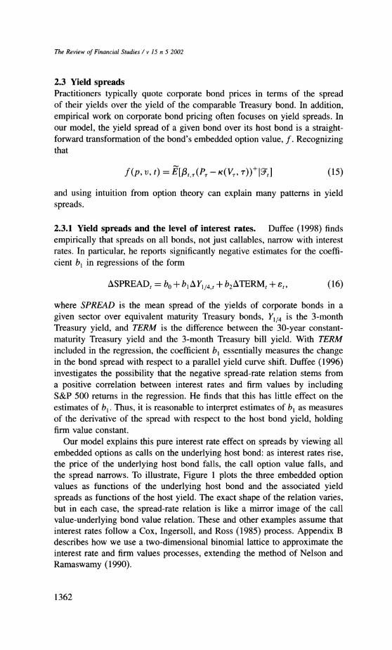
Our model explains this pure interest rate effect on spreads by viewing all

embedded options as calls on the underlying host bond: as interest rates rise, the price of the underlying host bond falls, the call option value falls, and

the spread narrows. To illustrate, Figure 1 plots the three embedded option values as functions of the underlying host bond and the associated yield

spreads as functions of the host yield. The exact shape of the relation varies, but in each case, the spread-rate relation is like a mirror image of the call

value-underlying bond value relation. These and other examples assume that

interest rates follow a Cox, Ingersoll, and Ross (1985) process. Appendix B

describes how we use a two-dimensional binomial lattice to approximate the

interest rate and firm values processes, extending the method of Nelson and

Ramaswamy (1990).

1362


A. Option values vs. host bond price B. Yield spreads vs. host bond yield

210 -

9

140-

03~~~~ .J~~~~~If~~~~ ~70

?...........'"' ..'...... ??????????????....

0 , , , 0 , , ,

85 93 101 109 4 6 8 10

Figure 1

Option values and yield spreads Three 5-year, 6.25%-coupon bonds: The gray line represents the callable defaultable, the black line represents the pure defaultable, and the dotted line represents the pure callable. Callable bond is currently callable at

par. The default payoff to bond holders is firm value. Call and default policies minimize bond values. The

instantaneous interest rate follows dr = K(fL - r) dt + rfr/rdZ; K = 0.5, fL = 6.8%, ao = 0.10. Firm value

follows dV/V = (r - y) dt + dW; y = 0.0, 4 = 0.20, V0 = 143. The instantaneous correlation between

the interest rate and firm value processes is zero. Numerical approximations use a two-factor binomial lattice.

Duffee (1998) documents three other empirical patterns. First, the negative spread-rate relation is usually stronger for callables. Second, among non-

callables, the relation is stronger for lower grade bonds. Third, for callables, the relation is stronger for higher priced bonds. We explain these patterns by

linking the spread-rate slope to the call option delta, f . Letting s Yx - YH

denote the spread between the yields of a given bond and its host and

assuming f is differentiable, we have

dsx = (1- dfx dp/dyH -1. (17) dyH dp dpx/dyx

We emphasize that the derivative dy- is taken holding firm value constant.

The terms -dp and dPx are derivatives of the same price-yield function, but dYH dyx

evaluated at different points, so they differ only because of the convexity of the price-yield function. In particular, percentage changes in their ratio are

small relative to percentage changes in 1 - df, so variation in the spread-rate

slope is driven by variation in the call option delta. The embedded call option delta ddf tends to be larger when the option is deeper in the money. That is

the case when either the strike price is lower, because of a call provision or because firm value is lower, or when the underlying host bond price is

higher. This would explain the three empirical patterns listed above.

The connection between the spread-rate slope and the option delta indi-

cates that the spread-rate slope is related to bond hedging. We develop this

point in section 4.1.1, where we draw a link between the spread-rate slope and duration. We also explain why the negative spread-rate relation is not

uniformly stronger for callables.

1363


In the model of Longstaff and Schwartz (1995), spreads also narrow with

interest rates, but through a different mechanism. There, default occurs when

firm value falls to an exogenous boundary, and in that event, bond holders

receive a fraction of the value of the host bond. As interest rates rise, the

drift of firm value under the risk-neutral measure increases, decreasing the

probability of default, and this causes spreads to decline. This effect of a rate

increase on V is at work in our model as well, but in addition, in our model, the rate increase narrows spreads by reducing P. By contrast, in the Longstaff and Schwartz model, the reduction in P by itself may actually serve to widen

spreads because it reduces the expected default payoff to bond holders.

2.3.2 Yield spreads and interest rate volatility and correlation. Existing models of corporate debt with endogenous default policies treat interest rates

as constant. In the example of Brennan and Schwartz (1980), the assumption of constant interest rates has only a small effect on bond value. Similarly,

Kim, Ramaswamy, and Sundaresan (1993) report that in their examples,

spreads are fairly insensitive to the level of interest rate risk or correla-

tion with firm value. However, such results do not generalize. Introducing stochastic interest rates can materially affect pricing.

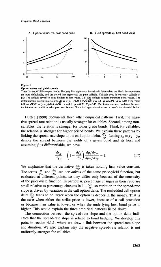
To understand the impact of an increase in interest rate volatility on corporate spreads, it is again useful to view the spread as a transformation of the

value of the issuer's option. From Equation (15), the corporate issuer's option value should increase in the volatility of P - V. The effect of an increase in

interest rate volatility on the volatility of P- V depends on the correlation p between r and V. When p > 0, interest rate volatility increases the volatility of P- V and widens spreads. However, when p < 0, P hedges changes in

V, and, if the volatility of P is low, an increase in the volatility of P can

improve this hedge, decreasing the volatility of P - V. Consequently, for

negative values of p, option values and corporate yield spreads can decline

as interest rate volatility rises. Figure 2 illustrates both cases.

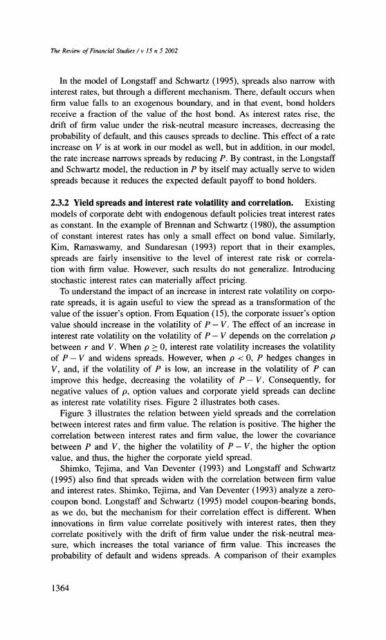
Figure 3 illustrates the relation between yield spreads and the correlation

between interest rates and firm value. The relation is positive. The higher the

correlation between interest rates and firm value, the lower the covariance

between P and V, the higher the volatility of P - V, the higher the option

value, and thus, the higher the corporate yield spread.

Shimko, Tejima, and Van Deventer (1993) and Longstaff and Schwartz

(1995) also find that spreads widen with the correlation between firm value

and interest rates. Shimko, Tejima, and Van Deventer (1993) analyze a zero-

coupon bond. Longstaff and Schwartz (1995) model coupon-bearing bonds,

as we do, but the mechanism for their correlation effect is different. When

innovations in firm value correlate positively with interest rates, then they correlate positively with the drift of firm value under the risk-neutral mea-

sure, which increases the total variance of firm value. This increases the

probability of default and widens spreads. A comparison of their examples

1364


A. Correlation = 0 B. Correlation = -0.5

260-

0 0.05 0.1 0.15 0 0.05 0.1 0.15

Figure 2

Yield spreads vs. interest rate volatility Two 10-year, 9%-coupon corporate bonds-one noncallable, represented by the black line, and one callable

at par, represented by the gray line. Call and default policies minimize bond values. The instantaneous

interest rate follows dr = K(C - r) dt + arfrdZ; K = 0.5, u = 9%, r0 = 9%. Firm value follows dV/V =

(r - y) dt + d W; y = 0.05, - = 0.15, V0 = 93. p is the instantaneous correlation between the interest rate

and firm value processes. Numerical approximations use a two-factor binomial lattice.

with ours suggests that the magnitude of the correlation effect is smaller in

their model. One reason for this may be the difference in assumptions about

default payoffs. In the event of default, bond holders in the Longstaff and

Schwartz model get a fraction of host bond value, not the value of the firm.

This means that the higher the correlation between interest rates and firm

value, the higher the expected default payoff, which should by itself narrow

spreads.

350

275

-0.5 0 0.5

Figure 3 Yield spreads vs. interest rate correlation with firm value Two 10-year, 9%-coupon corporate bonds-one noncallable, represented by the black line, and one callable at par, represented by the gray line. Call and default policies minimize bond values. The instantaneous interest rate follows dr = K((L - r) df + aordZ; K = 0.5, j, = 9%, r0 = 9%. Firm value follows dV/V =

(r - y) dt + -dW; y = 0.05, 4- = 0.15, V0 = 93. p is the instantaneous correlation between the interest rate and firm value processes. Numerical approximations use a two-factor binomial lattice.

1365


135 -

125 -

Critical

host l -115 -.---....

bond

price 105 -

95 -

85 I

72 86 100 114 128 142

Firm value

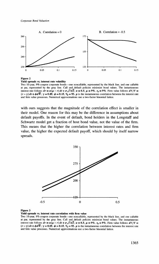
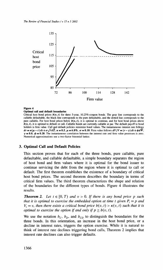
Figure 4

Optimal call and default boundaries Critical host bond prices b(v, t) for three 5-year, 10.25%-coupon bonds. The gray line corresponds to the callable defaultable, the black line corresponds to the pure defaultable, and the dotted line corresponds to the

pure callable. For host bond prices below b(v, t), it is optimal to continue, and for host bond prices above b(v, t), it is optimal to default or call. Callable bonds are currently callable at par. The default payoff to bond holders is firm value. Call and default policies minimize bond values. The instantaneous interest rate follows dr = K(IJ - r) dt + orfdZ; K = 0.5, it = 6.8%, ar = 0.10. Firm value follows dV/V = (r - y) dt + 4.dW; y = 0.0, 4 = 0.20. The instantaneous correlation between the interest rate and firm value processes is zero. Numerical approximations use a two-factor binomial lattice.

3. Optimal Call and Default Policies

This section proves that for each of the three bonds, pure callable, pure defaultable, and callable defaultable, a simple boundary separates the region of host bond and firm values where it is optimal for the bond issuer to

continue servicing the debt from the region where it is optimal to call or

default. The first theorem establishes the existence of a boundary of critical

host bond prices. The second theorem describes the boundary in terms of

critical firm values. The third theorem characterizes the shape and relation

of the boundaries for the different types of bonds. Figure 4 illustrates the

results.

Theorem 2. Let t E [0, T) and v > O. If there is any bond price p such

that it is optimal to exercise the embedded option at time t given P, = p and

V, = v, then there exists a critical bond price b(v, t) > K(v, t) such that it is

optimal to exercise the option if and only if p > b(v, t).

We use the notation bc, bD, and bcD to distinguish the boundaries for the

three bonds. In this orientation, an increase in the host bond price, or a

decline in interest rates, triggers the option exercise. While it is natural to

think of interest rate declines triggering bond calls, Theorem 2 implies that

interest rate declines can also trigger defaults.

1366


Models with constant interest rates describe the optimal call and default

rules in terms of critical firm values, a lower critical firm value below which

default is optimal and an upper critical firm value above which call is optimal

[see, for example, Merton (1974), Black and Cox (1976), and Leland (1994,

1998), and Goldstein, Ju, and Leland (2000)]. Our next result states that this

characterization is also valid when interest rates are stochastic, only now the

critical firm values are functions of interest rates.

Theorem 3. Let t E [0, T) and p > 0.

1. For the pure defaultable bond, there exists a criticalfirm value VD(p, t) <

p such that, at time t, given Pt = p and Vt = v, it is optimal to default

if and only if v < VD(P, t).

2. For the callable defaultable bond, there exists a critical firm value

VcD(P, t), satisfying VcD(p, t) < k and cD(p, t) < p, such that, at

time t, given Pt = p and Vt = v, it is optimal to default if and only

if v < VcD(p, t). In addition, if there exists any firm value v at which it

is optimal to call, then there exists a critical firm value vcD(p, t) > kt such that it is optimal to call if and only if v > VCD(p, t).

The next theorem describes the shape and relation of the different boundaries.

Theorem 4. For each t E [0, T),

1. v1 < V12 = bD(v, t)< bD(V2, t).

2. p < P2 = VD(Pl, t) < VD(P2, t). 3. v1 < V2 < kt, bcD(vl, t) < bD(2, t).

4. kt < v, < v2 = bcD(v,, t) > bCD(V2,.t). 5. v < k, = bCD(v, t) > b(v, t). 6. v > kt = bcD(v, t) > bc(v, t).

First, consider the default option embedded in the pure defaultable bond. Part 1 of Theorem 4 states that the critical bond price above which the firm should default, bD(v, t), is increasing in the firm value v. That is, the

higher the firm value, the lower the interest rates must be to trigger a default.

Conversely, Part 2 indicates that the critical firm value below which the equity holders should default is increasing in the host bond price p. In other words, in high interest rate environments, it takes lower firm values to make equity holders stop servicing the debt and give up the firm.

Next, consider the option to call or default embedded in a callable defaultable bond. For firm value below the call price, v < kt, exercising the option means defaulting. For firm value greater than the call price, v > kt, exercising means calling the bond. Part 3 of Theorem 4 indicates that the critical host bond price, bCD(v, t), above which it is optimal to default, is increasing in

v, like bD(v, t). Part 4 indicates that the critical host bond price, bcD(v, t), above which it is optimal to call, is decreasing in v. At lower firm values, it takes lower interest rates to trigger a bond call.

1367


Parts 5 and 6 of Theorem 4 describe the interaction of the call and default

options on the optimal exercise policy. Part 5 states that the callable default-

able has a smaller default region than the pure defaultable. Part 6 states

that the callable defaultable has a smaller call region than the pure callable.

When both options are present, the value of preserving one option can make

it optimal for the issuer to continue servicing the debt in states in which it

would otherwise exercise the other option. These results will be useful for

understanding the patterns in the risk measures presented below.

4. Hedging Interest Rate Risk and Credit Risk

A corporate bond is subject to both bond market risk and firm risk. In prin-

ciple, a portfolio containing Treasuries and shares of the issuer's equity could

serve to hedge both risks. The number of units of these instruments in the

hedge portfolio, the hedge ratios, explicitly spell out the trading strategy for

hedging and quantify the exposure to risks that the corporate bond imparts. The market for the issuer's equity is generally much more active than the

market for the firm's assets, so the hedge ratios in a hedge using host bonds

and equity have more practical application than the hedge ratios in a hedge

using host bonds and firm assets. However, the two pairs of hedge ratios

are related through a simple transformation, and we find that their dynamics are qualitatively very similar. For ease of exposition, we work with the host

bond-firm value hedge, because its dynamics can be understood through a

more direct application of our model.

We use a bond's hedge ratio with respect to firm value, d, to measure its

firm risk. However, instead of using a bond's hedge ratio with respect to the

host bond, dP, to measure its bond market risk, we use a similar but more dp

widely recognized risk measure,

duration dp x

(18) dyH

The measures dpx/px and dpx behave similarly because their dynamics dyH dp

are both driven by the dynamics of the option delta dfx. More precisely, dp

dpxpyH = dp

dy-PL ) and the percentage changes in the factor (-d-p ) dyH dp dYH Pxp dYH Px

associated with changes in firm value and interest rates are small relative

to the percentage changes in dPx = 1 - dpL The duration defined in Equa- tion (18), sometimes called "effective duration," essentially measures price

sensitivity to Treasury yields. By contrast, so-called "modified duration,"

_dpx/pxx measures a bond's price sensitivity to its own yield. Both mea- dyx

'

sures are used by practitioners, but effective duration is generally a more

appropriate measure to use for risk management.

1368


A. Duration vs. host bond price B. Duration vs. firm value

5 -_ 6-

4-

3-

3

2- 2-

1- 1

0 , , , ,

95 105 115 125 135 85 110 135 160

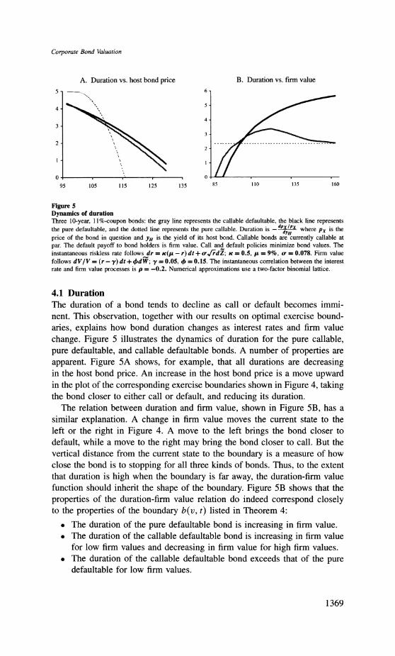
Figure 5

Dynamics of duration

Three 10-year, 11%-coupon bonds: the gray line represents the callable defaultable, the black line represents the pure defaultable, and the dotted line represents the pure callable. Duration is - dpX/Px where Px is the

dyH price of the bond in question and YH is the yield of its host bond. Callable bonds are currently callable at

par. The default payoff to bond holders is firm value. Call and default policies minimize bond values. The

instantaneous riskless rate follows dr = K(,L - r) dt + orirdZ; K = 0.5, pI = 9%, a = 0.078. Firm value

follows dV/V = (r - y) dt + <idW; y = 0.05, - = 0.15. The instantaneous correlation between the interest

rate and firm value processes is p = -0.2. Numerical approximations use a two-factor binomial lattice.

4.1 Duration

The duration of a bond tends to decline as call or default becomes immi-

nent. This observation, together with our results on optimal exercise bound-

aries, explains how bond duration changes as interest rates and firm value

change. Figure 5 illustrates the dynamics of duration for the pure callable,

pure defaultable, and callable defaultable bonds. A number of properties are

apparent. Figure 5A shows, for example, that all durations are decreasing in the host bond price. An increase in the host bond price is a move upward in the plot of the corresponding exercise boundaries shown in Figure 4, taking the bond closer to either call or default, and reducing its duration.

The relation between duration and firm value, shown in Figure 5B, has a

similar explanation. A change in firm value moves the current state to the

left or the right in Figure 4. A move to the left brings the bond closer to

default, while a move to the right may bring the bond closer to call. But the

vertical distance from the current state to the boundary is a measure of how

close the bond is to stopping for all three kinds of bonds. Thus, to the extent

that duration is high when the boundary is far away, the duration-firm value

function should inherit the shape of the boundary. Figure 5B shows that the

properties of the duration-firm value relation do indeed correspond closely to the properties of the boundary b(v, t) listed in Theorem 4:

* The duration of the pure defaultable bond is increasing in firm value.

* The duration of the callable defaultable bond is increasing in firm value

for low firm values and decreasing in firm value for high firm values.

* The duration of the callable defaultable bond exceeds that of the pure defaultable for low firm values.

1369


* The duration of the callable defaultable bond exceeds that of the pure callable for high firm values.

These last two points describe an interaction effect on duration: a call provision by itself reduces duration, as does default risk by itself, but a call

provision can increase the duration of a defaultable bond and default risk

can increase the duration of a callable bond because the presence of one

option delays the exercise of the other.

4.1.1 Duration and the slope of the spread-rate relation. The slope of

the spread-rate relation studied empirically by Duffee (1998) and described

in Section 2.3.1 is related to duration through the following equation.

dPx/Px

dsx - dypx _ - duration,. dH - 1. (19)

dyH dpx/Px modified durationx

dyx

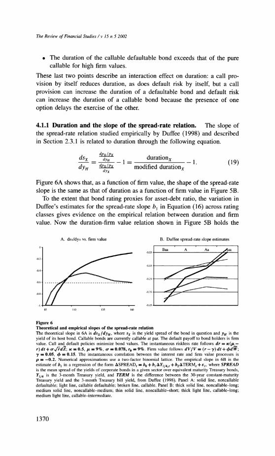
Figure 6A shows that, as a function of firm value, the shape of the spread-rate

slope is the same as that of duration as a function of firm value in Figure 5B.

To the extent that bond rating proxies for asset-debt ratio, the variation in

Duffee's estimates for the spread-rate slope bl in Equation (16) across rating classes gives evidence on the empirical relation between duration and firm

value. Now the duration-firm value relation shown in Figure 5B holds the

A. dsx/dyH vs. firm value B. Duffee spread-rate slope estimates

Baa A Aa aa -0.05

-0.2-

-0.15

-0.4

-0.25

-0.6.

-0.8-035 /0.3

-1 , , , -0.45

85 110 135 160

Figure 6 Theoretical and empirical slopes of the spread-rate relation

The theoretical slope in 6A is dsx dyH, where sx is the yield spread of the bond in question and YH is the

yield of its host bond. Callable bonds are currently callable at par. The default payoff to bond holders is firm

value. Call and default policies minimize bond values. The instantaneous riskless rate follows dr = K(I -

r) dt + ar'ddZ; K = 0.5, IL = 9%, a- = 0.078, r0 = 9%. Firm value follows dV/V = (r - y) dt + OdW;

y = 0.05, - = 0.15. The instantaneous correlation between the interest rate and firm value processes is

p = -0.2. Numerical approximations use a two-factor binomial lattice. The empirical slope in 6B is the

estimate of bl in a regression of the form ASPREADt = bo + b AY1/4,t + b2ATERMt + Et, where SPREAD

is the mean spread of the yields of corporate bonds in a given sector over equivalent maturity Treasury bonds,

Y1/4 is the 3-month Treasury yield, and TERM is the difference between the 30-year constant-maturity

Treasury yield and the 3-month Treasury bill yield, from Duffee (1998). Panel A: solid line, noncallable

defaultable; light line, callable defaultable; broken line, callable. Panel B: thick solid line, noncallable-long; medium solid line, noncallable-medium; thin solid line, noncallable-short; thick light line, callable-long; medium light line, callable-intermediate.

1370


bond coupon rate constant, while in the data, coupon rates decline as rating increases. However, examples suggest that if coupon rate varies to keep all

bonds priced at par, then the noncallable bond duration remains upward-

sloping in firm value, although the callable bond duration becomes flat at

zero because the bonds are callable at par. The data most likely reflect a

mixture of these cases. Coupon rates decline with rating, but not by so much

that all bonds are at par. Lower rating classes contain more discount bonds

and higher rating classes contain more premium bonds.

Figure 6B plots Duffee's (1998) estimates for b1 for various bond rating classes within a given maturity sector. Like the duration-firm value graphs in

Figure 5B, the curves for noncallable bonds are upward-sloping, while the

curves for callable bonds are hump-shaped. Again, our model's explanation for these shapes lies in the shape of the endogenous default and call bound-

aries analyzed in Theorem 4 and illustrated in Figure 4. As bonds move

away from default, the sensitivity of spreads to rates moves toward zero, but

as callable bonds approach call, this sensitivity becomes large again.

4.1.2 Duration in models with exogenous default boundaries. In cor-

porate bond models with exogenous default boundaries, default occurs when

firm value falls to a pre-specified critical level [see, for example, Brennan and

Schwartz (1980), Kim, Ramaswamy, and Sundaresan (1993), Longstaff and

Schwartz (1995), and Brys and de Varenne (1997)]. If the model specifies a fixed payoff to bond holders in the event of default, then, in states when

host bond prices are lower than this level, default can be a windfall to bond

holders and bond spreads can become negative. Instead of specifying a fixed

default payoff to bond holders, most exogenous default models set the bond

default payoff equal to a fraction 8 of the host bond price, which guaran- tees that default is not a benefit to bond holders [see, for example, Kim,

Ramaswamy, and Sundaresan (1993) and Longstaff and Schwartz (1995)]. This, however, makes duration a sort of U-shaped function of firm value

near default. Duration increases not only as firm value rises and the bond

becomes like a nondefaultable, but also as firm value falls to the default

level, and the bond tracks the host bond.

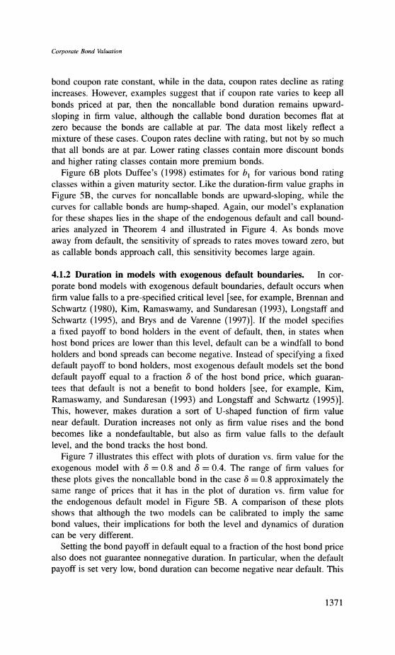
Figure 7 illustrates this effect with plots of duration vs. firm value for the

exogenous model with 8 = 0.8 and 8 = 0.4. The range of firm values for

these plots gives the noncallable bond in the case 8 = 0.8 approximately the

same range of prices that it has in the plot of duration vs. firm value for

the endogenous default model in Figure 5B. A comparison of these plots shows that although the two models can be calibrated to imply the same

bond values, their implications for both the level and dynamics of duration

can be very different.

Setting the bond payoff in default equal to a fraction of the host bond price also does not guarantee nonnegative duration. In particular, when the default

payoff is set very low, bond duration can become negative near default. This

1371


A. Default payoff = 0.8 x host bond price B. Default payoff = 0.4 x host bond price

6-

5-

4- \4 4-

3- 3- _-

2- 2-

1- I1

0 , , 0

220 300 380 460 220 300 380 460

Figure 7

Duration vs. firm value in exogenous default model

Three 10-year, 11%-coupon bonds: the gray line represents the callable defaultable, the black line represents the pure defaultable, and the dotted line represents the pure callable. Duration is - dpX/p where Px is the

price of the bond in question and YH is the yield of its host bond. Callable bonds are currently callable at par. Default occurs when firm value hits 220. The default payoff to bond holders is a fraction of the host bond

price. Call policies minimize bond values. The instantaneous riskless rate follows dr = K(, - r) dt + oa,fdZ; K = 0.5, It = 9%, a = 0.078, ro = 9%. Firm value follows dV/V = (r - y) dt + 4dW; y = 0.05, = = 0.15.

The instantaneous correlation between the interest rate and firm value processes is p = -0.2. Numerical

approximations use a two-factor binomial lattice.

is because increases in interest rates increase the drift of firm value, reducing the risk of default. Near default, the benefit of reducing the risk of default, which is catastrophic when the default payoff is very low, offsets the cost of

the loss in the value of the bond's future promised payments.

By contrast, part 3 of Theorem 1 implies that duration is always nonnegative in our model. Table 1 compares the durations of bonds under the two

models. The two bonds have the same coupon, maturity, and price, but bond

duration is positive under the endogenous bankruptcy model and negative under the exogenous bankruptcy model. Again, the two models can imply the same bond price and yet have very different implications about hedging. More generally, in the presence of stochastic interest rates, it seems difficult

to devise an exogenous default specification that has both the same pricing and same hedging implications as the endogenous model.

Table 1

Duration under alternative bankruptcy assumptions

Default Default Coupon Yield

boundary payoff Maturity rate spread Duration V0 E{VIat default}

Endogenous V 10 years 9% 720 bp 0.8 65 60

Exogenous 0.2 x P 10 years 9% 720 bp -0.6 118 75

Both bonds are noncallable. P is the price of the noncallable, nondefaultable host bond with the same coupon and maturity.

Duration is dppX where Px is the price of the bond in question and YH is the yield of its host bond. The instantaneous riskless

rate follows dr = K(/ - r) dt + ao/dZ; K = 0.5, u = 9%, o- = 0.078, ro = 9%. Firm value follows dV/V = (r - y) dt + 4dW;

y = 0.12, ( = 0.15. The instantaneous correlation between the interest rate and firm value processes is p = -0.2. Numerical

approximations use a two-factor binomial lattice.

1372


A. Bond sensitivity to firm value vs. host bond price

1 -

0.8 -

0.6-

0.4-

0.2 -

95 105 115 125

B. Bond sensitivity to firm value vs. firm value

0.8

0.6

0.4

0.2

90 130 170 210 250

Figure 8

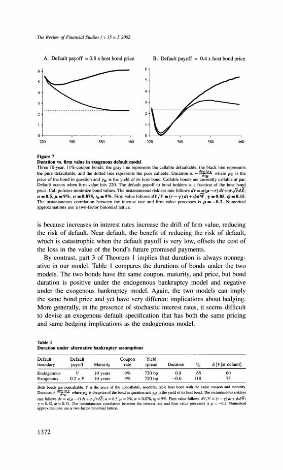
Dynamics of bond sensitivity to firm value Two 10-year, 11%-coupon corporate bonds. One bond is noncallable, represented by the black line, and one

bond is callable at par, represented by the gray line. Bond sensitivity to firm value is x where Px is the price of the bond in question and v is firm value. The default payoff to bond holders is firm value. Call and default

policies minimize bond values. The instantaneous riskless rate follows dr = Kc(I - r) dt + orf/rdZ; K = 0.5,

It = 9%, ao = 0.078. Firm value follows dV/V = (r - y) dt + bdW; y = 0.05, 4 = 0.15. The instantaneous correlation between the interest rate and firm value processes is p = -0.2. Numerical approximations use a two-factor binomial lattice.

4.2 Bond price sensitivity to firm value

A bond's sensitivity to firm value is high when default is imminent and low when call is imminent. Therefore, we can again use the results on optimal call and default boundaries in Theorem 4 to explain the dynamics of hedging credit risk. Figure 8 plots corporate bond sensitivity to firm value as a function of the host bond price and as a function of firm value. Three effects are clear.

* The sensitivity of the noncallable bond increases in the host bond price, because increases in the host bond price bring the bond closer to default.

* The sensitivities of both the noncallable and callable bonds decrease in firm value, because as firm value rises, both bonds move away from the default boundary.

* The callable bond's sensitivity to firm value is uniformly lower than that of the noncallable,

because the callable bond is always farther from the default boundary. This last effect suggests that the presence of a call provision mitigates the underinvestment problem of levered equity. As Myers (1977) shows, since levered

equity holders share increases in firm value with bond holders, they may pass up positive net present value projects that require all-equity financing. By increasing equity sensitivity to firm value, the call provision makes the underinvestment problem less severe.

5. Conclusion

This paper analyzes corporate bonds in a model in which the interest rate is a one-factor diffusion process and the issuer follows optimal call and default rules. By incorporating both stochastic interest rates and endogenous

1373

I .


bankruptcy, the model bridges a gap in the corporate bond literature. The

combination of these elements is of particular interest because bankruptcy

assumptions significantly impact interest rate hedging. A single framework encompasses the callable defaultable bond and its pure

callable and pure defaultable counterparts, viewing each bond as a riskless,

noncallable host bond minus a call on that host bond. This perspective provides intuition for the sensitivity of spreads to interest rate levels, volatility, and correlation with firm value. It also leads us to extend results for callable

bonds to defaultable bonds.

The paper develops analytical results on corporate bond valuation and

optimal call and default boundaries. Previous corporate bond models that

provide analytical results with stochastic interest rates either work with a

zero-coupon bond or else treat bankruptcy as exogenous, and thus avoid the

issue of optimal default rules. By characterizing the solution to the two-

dimensional optimal stopping time problem analytically, this paper makes an

incremental theoretical contribution.

The optimal exercise boundaries explain the dynamics of hedging. For

example, the critical host bond price above which it is optimal to exercise

the embedded option is an increasing function of firm value for noncallable

bonds. For callable bonds however, it is an increasing function at low firm

values and a decreasing function at high firm values. This explains why non-

callable bond duration is an increasing function of firm value while callable

bond duration is a hump-shaped function of firm value. By contrast, under

typical exogenous bankruptcy specifications, duration is a U-shaped function

of firm value near default.

We interpret recent evidence on the relation between corporate bond yield

spreads and Treasury bond yields as information about hedging and find that

the empirical patterns in the spread-rate slope mirror the duration patterns

implied by endogenous bankruptcy. In particular, our results on boundaries

and durations explain why the slope of the empirical spread-rate relation is

increasing in bond rating for noncallables, but hump-shaped for callables.

A formal empirical test of the model's hedging implications would be an

interesting subject for future research.

Much of the recent work in the corporate bond literature has focused on

optimal or strategic behavior in the presence of frictions such as taxes or

bankruptcy costs. In order to focus on optimal issuer behavior with stochastic

interest rates, our paper uses a relatively simple contingent claims approach that abstracts from such frictions. One extension would be straightforward, however. For expositional purposes, the model presented here assumes that

in the event of default, bond holders get the full value of the firm V and

equity holders get nothing. Yet we could easily incorporate deviations from

absolute priority of the following form: in the event of default, bond holders

1374


get a V and equity holders get (1 - a)V, where a is a constant between zero

and one. In that case, corporate bond values would become

Px(P,, t)= - fx(p, av, t)= px(p, av, t). (20)

Bond prices, yields, and durations would be invariant to a holding av con-

stant and sensitivity to firm value would adjust in a straightforward fashion.

All of our analytical results would continue to hold, as would the qualitative nature of our numerical results.

This paper focuses on how changes in market conditions affect prices,

spreads, durations, hedge ratios, and call and default decisions in the absence

of frictions. However, many other issues surround the subject of corporate debt. One area of interest is term structure. Another is the dynamics of

optimal capital structure with taxes, bankruptcy costs, and refinancing costs.

The framework developed here could provide the foundation for research in

a variety of different directions.

Appendix A: Proofs

The proof of Theorem 1 makes use of a number of so-called no-crossing properties. The first

follows from Proposition 2.18 of Karatzas and Shreve (1987):

Proposition 2. Consider two values of interest rates at time 0, ro') and r(2) such that r0') < r2), and denote the corresponding interest rate processes as rtI) and rt, respectively. Then

[r(1) < r2, 0 < t < oo] =1. (21)

This no-crossing property of r implies no-crossing properties for /3, P, 3P, and V. For ease of

exposition, let

/3 - P3o,, (22)

Corollary 1. Let pj,) and 312) be the discount factor processes corresponding to initial interest

rates r'l) and r2), respectively. Then

rI) < ro2) ==0 PI' > p(2), 5-a.s. V 0 < t < oo. (23)

Proof. From Proposition 2, we have rsl) < r(2), V 0 < s < t. The paths of r(') and r(2) are

continuous, so there exists a neighborhood around t = 0 on which r() < r(2). Consequently,

e-o rs1)ds e- sr(2)ds

The monotonicity of the host bond price in level of the interest rate implies:

Corollary 2. r) < P r (2) p(l) > p'(2), f-_ a.s. V O< t < T.

Combining Corollaries 1 and 2 yields:

Corollary 3. r 0) < r(2) = /3I)p(l) > /2)p(2), _ a.s. V 0 < t < T.

1375


Under the firm value specification (4),

V, = Vo. ef rudu-fo du- f o du+fo ju dWu (24)

It follows that:

Corollary 4. r) < (r2) = V,(') < Vt(2), -a.s. V 0 < t < T.

The following lemma also serves in the proof of Theorem 1.

Lemma 1. ro) < r E2) = E[pt2 )pt() ] > p(2)p _ p(l) V 0 t < T.

Proof. Define the P-martingale f3P* by

1P, ^ f

C ,Tds+l AT19]

1 , ?

VO<t<T. (25)

Note that

1,P, =E [c f1ds + 1 T , (26)

so

PtP = ftPt + c fs ds. (27)

Rearranging,

/3P,-Po = tP,*-c j 3t dt- P (28) o

E[13,P,]- Po = -E[c f , ds]. (29)

Corollary 1 implies that

[Icf (1)ds]> E[ c (2)dsJ (30)

and the result follows. U

Proof of Theorem 1. 1. Consider the stopping problem at time t < T. Let p(1) > p(2) be two

possible values of the time t bond price. Note that, from the strict monotonicity of PH(-, t), there are corresponding values of the time t interest rate process, rM( and r(2), satisfying

r() < r(2). Let r be the optimal stopping time given the state at time t is P, = p(2) and

V, = v. Then its feasibility as a stopping time for the state Pt = p(l) and V, = v implies that

f(p('), v , t) f( E>[,13 (P( - K(V( ), 7))

-^{PT - K t} (31) -

p-( p(V2'

- K(V(2), T))+

I] (3t1)

> 0. (32)

To establish the last inequality, note that if T = t, the expectation above is p(l) - p(2) > 0.

If T > t, r(l) < r(2) = j,l) > 8(2), and p() > p .2). Furthermore, Corollary (4) implies that

K(V,('), ) < K(V(2) ). It follows that (P() -K(V(1), ))+ > (P(2)- K(V(2, ))+. Now

p(2) K(V2), r) > 0 with positive probability, so p,, T(P( -

K(V,1), r))+ > P -

K(VT2, r)) a.s. and ,(PT K(V ) T)) > t 2)(P 2)-K(VT2) , ))+ with positive

probability.

1376


2. Consider the cases K(V,, t) = V, and K(Vt, t) = k, A V, and let t < T. Let v(l < v(2) be two

possible values of the time t firm value, V,. From Equation (24), V(l) < V(2), Vs e [t, T]. It follows that K(V(I), T) < K(V2), r), where r is the optimal stopping time given that the

state at time t is P, = p and V,= v(2). The feasibility of T as a stopping time for the state

P, = p and V, = v() implies that

f(p, v), t) - f(p, v(2), t) > E[At,T(P,

- K(V!), T))+

- ,,(P - K(V(2), 7)) +It] (33)

> 0. (34)

In the case of the pure default option, K(V,, t) = V,, the last inequality is strict.

3. We let p(l) > p(2) and prove that f(p(2), v, t) -

f(p(l), , t) > p(2) _ p(l). Let r() < r(2)

denote the time t interest rates corresponding to the two possible values for the time t

bond price, p(l) and p(2), respectively. Let r be the optimal stopping time for p('). Then r

is a feasible stopping time for p(2) as well.

f(p(2)v, ,t)-f(p(l), v, t)

> E[t 2) (p(2) K(V(2), 7))+ -

)(P,) K(VTI', ))+ t] (35)

( (2) (PT(2) (V2) _ ()(P(l - K l) )) t,(P -K(VT , )) -(V1), T))]

1 (P()>K(v(1) )) ) (36)

> E [(2, (p(2 - K(V(2), T)) - (() K(V(', ))]

+L t, ) - r t), r)] ()( )) (38)

1 (P( i K ( ),)( i) T)) I }t (39)

-

pR(2)_ p(2) P4() 1

= ()

(1, (1( 41)

K(V , ) < K(V2, ) (Corollary 4) which in turn imply that P) < K( ), r) = P(2)

K(V2) T). Inequality (39) follows from the fact that r((l < r)> ( () (V,), t)

,B(2K(V4r2),) (Corollary 1 and Equation 24). Inequality (40) follows from the fact that

r(1) < r(2) ?. /3(,4P4) > f3,)P4() (Corollary 3). Finally, Inequality (41) follows from Lemma 1.

4. We let > and prove that f(p, ) (2) - ), ) Let be the optimal

stopping time for ). Then r is a feasible stopping time for v(3.

= E [[t, r -

K(V (1)) -

1,(PV T K) ))]

> (K((2) v)()) pT 1 | (43)

- t, T 7 rt, T1 (40)

)P(2)- (1)~ (41)

Equation (36) follows from the fact that r(l) < r(2) =:i p(l) > pT(2) (Corollary 2), and

K(VT(,), '

) < ,

K ) (Corollary 4) which in turn imply that PT(') _ V~(') r) = P?)_

K(V?), T

). Inequality (39) follows from the fact that r(l)< r(2 = KV,--, T).. /3(2)K( V, T) (Corollary 1 and Equation 24). Inequality (40) follows from the fact that

r(l) < r(2) =:=,t,8(1)p) >?2)p(2) (Corollary 3). Finally, Inequality (41) follows from Lemma 1. t,T T -t , ,

'r

4. We let v(2) > v(0) and prove that f(p, v(2), t) -f(p, v(1), t) > v(l) - V(2). Let r be the optimal

stopping time for v(0. Then T is a feasible stopping time for v(2).

f(p, v(2', t)- f(p, v(1), t) >/~[/,~(P1- K(V?2), r))+

-~t([B,.1(P1--K(V(2), r))+ _t - K(VK(V ) T))]

.' (PT > K (VT('), T)) I Yt

1 (43)

1377


l(P,>K(V(l),))I1tl (44)

-I[,,,(K (VT(", 'r) - K (VT('), r))] I (PT>K(V,1),T)) ty' (45)

> f[PIc(K(VTI'), r) - K(VT2), r)) IJ] (46)

( E

') _V1) V(2))1~ (47)

= e ft yu du (V(I) - v(2) (48)

> VM - v(2) (49)

Inequalities (43) and (46) follow from the fact that v12 > V(I) =j K(VT2), r) > K(V('),T r). U

Proof of Proposition 1. The first inequality is obvious. We establish the second inequality as

follows.

fCD(P, v,It) = sup E[,t,T(PT - kTA VT)+IYt] (50) t<Tr<T

= sup E{ft T((PI - k) V (PI - VX))IJt] (51) t<r<T

< sap K[Pt,,((PT- k,)+ + (P, - VT)+)IYJ] (52) t<T<T

< sup 'E[01,JPT l ] + sup E[I3T(PT VT) + 1] (53) t<T<T t(<r<T

- fM(P, v, t) +fD(p, v, t). (54)

For the proofs of Theorems 2-4, note that the continuation region for each option is the open

set

U {(p, v, t) E R+ x R1 x [0, T]: f(p, v, t) > (p - K(V, t))+I. (55)

In addition, note that for all t e [0, T), f(p, v, t) > 0.

Proof of Theorem 2. Suppose it is optimal to continue at p, and p, > P2- We show that it is

then optimal to continue at P2- Using the call delta inequality, we have

f (P2, VI t) >- f (PI IVI t) + P2 - PI > (PI - K(V, tW) + P2 - PI >- P2 - K(V, t). (56)

In addition, f(p2, v, t) > 0, SO

f (P21 VI t) > (P2 - K(V, t) (57)

Let b(v, t) be the supremum of p such that (p, v, t) E U. The point (b(v, t), v, t) cannot

lie in U because U is open, so f(b(v, t), v, t) = b(v, t) - K(V, t) > 0, which implies b(v, t) >

K(V, t). U

Proof of Theorem 3. 1. Note that it must be optimal to default at v = 0. Suppose it is

optimal to continue at v1 and v, < v2. We show that it is then optimal to continue at v2.

Using the put delta inequality,

f (PI V21 t) >- f (p, VII t) + VI - V2 > (P - VX ) + VI - V2 >- P - V21 (58)

1378


and thus f(p, V2, t) > (p- v2)+. Let VD(p, t) be the infimum of v such that (p, v, t) E U.

Since f(p, VD(p, t), t) > 0, VD(p, t) < p.

2. First, suppose it is optimal not to default at v, and v1 < v2. We show that it is then also

optimal not to default at v2. From the put delta inequality,

f(p,2, t) f (P, V,'+ t) v_- > (p- v kt)++v -2-

> P- 2, (59)

and thus f(p, v2, t) > (p- v2)+

Note that it must be optimal to default at v = 0. Therefore, there exists a critical value

VCD(P, t) such that it is optimal to default Vv, v < vcD(p, t). Further, CDo(p, t) < p must

hold. Otherwise f(p, Vco(p, t), t) = 0, a contradiction. In addition, VCD(p, t) < k, must

hold. Otherwise, there would exist a firm value greater than k, at which it is optimal to

default, which is impossible.

Next, suppose it is optimal to call at v,, and v, < v2. We show that then it is then optimal to call at v2. Note that k, < v, must hold. Now, on one hand, f(p, v2, t) > p - k, v2 =

p -k,. On the other hand, from part 2 of Theorem 1, f(p, v2, t) < f(p, vl, t) = p- k,. Let VCD(p, t) > kt be the minumum of v such that it is optimal to call at (p, v, t). ?

Proof of Theorem 4. 1. Suppose 0 < p < bD(v,, t). Then p < bD(v2, t) as well:

f(p, v2, t)> f(p, v,t) + v v2 > p-v + v -v2 = p-v2. (60)

2. Suppose v > vD(p2, t). Then v > vD(pl, t) as well:

f(Pl,v,t) > f(p2,v,t)+pI P2- >P2-V +Pl -P2 > P -v. (61)

3. The proof is essentially the same as that in part 1.

4. Suppose 0 < p < bc(v2, t). Then p < bc(vl, t) as well:

f(p, V,, t) > f(p, v2, t) > g(p, v2, t) = (p - kt)+ = g(p, vl,, t). (62)

5. If p <bD(v,t), then fco(p, v,t) > f(p, v, t)> p-v=p-vAk,, so p < bc(v, t). 6. If p<bc(v,t), then fco(p,v,t)> fc(p,t) >p-k,=p- vAk,, so p<bcD(v,t). ?

Appendix B: Numerical Implementation

Nelson and Ramaswamy (1990) show how to use binomial processes to approximate a general class of single-factor diffusions. To extend their analysis to multi-factor diffusion models, we

first transform the state variables into new diffusion processes that are uncorrelated and have

constant volatility. Then we construct a recombining, two-dimensional binomial lattice for the

resulting orthogonalized diffusions. Finally, we transform the lattice for the orthogonalized state

variables into a lattice for the original variables and price the callable and defaultable bonds using backward induction. This appendix describes the construction of the two-dimensional binomial

lattice. Other papers illustrating the implementation of bivariate diffusions are Boyle, Evnine, and Gibbs (1989), Hilliard, Schwartz, and Tucker (1996), who consider lognormal processes, and Hull and White (1994a,b, 1996), Ho, Stapleton, and Subrahmanyam (1995), and Peterson,

Stapleton, and Subrahmanyam (1998), who consider two-factor term structure models. As a special case of our model, we consider the Cox, Ingersoll, and Ross (1985) interest rate

process r,, where

dr, = K(, - r,) dt + ova,tdZ,. (63)

1379


Firm value V, follows the log-normal process

dV t = (r - y,) dt + ,d W, (64)

V,

The instantaneous correlation between Zt and W, is denoted as Pt. Note that y, > 0, 4, > 0, and

Pt E (-1, 1) are deterministic functions of time. To orthogonalize these interest rate and firm value processes, let G, - nt) and H, - 2rit

Then, by Ito's Lemma,

dG,=,atdt+dW,, , t = rt y , and

2t (65) r2

dH, = v,dt + dZ,, vt = K .Kr

Second, let X, = G, and Yt = - (-ptG, + Ht). Then X and Y are diffusions with unit

instantaneous variance and zero cross-variation. The drift of X is /,+ = /,t and the drift of Y is

'ut,- l (-PtA,t + vt)'

The inverse transformation to obtain r, and V, from X, and Y, are

Vt = e'iX, rt= [ .( 1 -p2 +tX)1 . (66)

To get a lattice for r and V, we apply this inverse transformation at each node of the lattice for

X and Y.

To construct a recombining, two-dimensional binomial lattice for the variables X and Y, we

divide the time-interval [0, T] into N equal intervals of length At. From a node (X,, Y,) at time

t, the lattice evolves to four nodes, (X+, Y+), (X+, Yt-), (X,, Yt+), and (X-, Yt-), where

X+ = X, + (2k, + 1)V/A, X = X, + (2kl - 1)V/. t t _(67) Y= Y, + (2k2 + 1)V/A, Y,- = Y, + (2k2 - 1)V,

and k and k2 are integers such that

(2k,- 1)vt </ L+At < (2k, + l)V/t, (68)

(2k2- 1) < /;-At < (2k2 + 1)V . (69)

The four nodes have associated risk-neutral probabilities pq, p(l - q), (1- p)q, and (1-

p)( - q), respectively. The probabilities, p, of an up-jump in X, process, and q, of an up-jump in Y, process, are picked to ensure the right first moments at the node (Xt, Yt):

P= +t -k,, q + -k2. (70) 2 2 2 2

Equations (68) and (69) ensure that the probabilities are between 0 and 1. While the first

moment of the process (X, Y) is matched exactly by the scheme above, the second moment

is approximated with an error that is O(At). The two-factor binomial process converges in

distribution to the original continuous-time process as At - 0.

To make the lattice for each state variable recombine, the variable can only move an integral number of increments /At, as Equation (67) indicates. When the drift terms A+ and /it are

large in magnitude, for instance, at low interest rates when the speed of mean reversion is high,

multiple jumps, that is, nonzero k, or k2, occur. However, the lattice for each variable has only

1380


n + 1 nodes at each time nAt, so an up or down move from any node at time (n - l)At must

lead to one of the n + 1 nodes at time nAt. Therefore, the moves described in Equations (68) and

(69) require that At be sufficiently small. The numerical examples employ 35 to 40 time steps

per year. We check the convergence by matching the price of a zero-coupon bond maturing at

T, which can be calculated analytically, and by matching the price of a European default option on the zero-coupon bond with an expiration at T, under the two-factor specification, which can

be calculated using Monte Carlo simulation.

References

Abken, P. A., 1993, "Valuation of Default-Risky Interest-Rate Swaps," Advances in Futures and Options Research, 6, 93-116.

Acharya, V. V., S. R. Das, and R. K. Sundaram, 2002, "Pricing Credit Derivatives with Rating Transitions," Financial Analysts Journal, 58(3), 28-44.

Acharya, V. V., J. Huang, M. G. Subrahmanyam, and R. K. Sundaram, 2002, "When Does Strategic Debt-

Service Matter?," working paper, London Business School.

Amin, K. I., and R. A. Jarrow, 1992, "Pricing Options on Risky Assets in a Stochastic Interest Rate Economy," Mathematical Finance, 2, 217-237.

Anderson, R. W., and S. Sundaresan, 1996, "Design and Valuation of Debt Contracts," Review of Financial

Studies, 9, 37-68.

Black, F., and J. C. Cox, 1976, "Valuing Corporate Securities: Some Effects of Bond Indenture Provisions," Journal of Finance, 31, 351-367.

Black, F., and M. Scholes, 1973, "The Pricing of Options and Corporate Liabilities," Journal of Political

Economy, 81, 637-654.

Boyle, P. P., J. Evnine, and S. Gibbs, 1989, "Numerical Evaluation of Multivariate Contingent Claims," The

Review of Financial Studies, 2, 241-250.

Brennan, M. J., and E. S. Schwartz, 1977a, "Convertible Bonds: Valuation and Optimal Strategies for Call

and Conversion," Journal of Finance, 32, 1699-1715.

Brennan, M. J., and E. S. Schwartz, 1977b, "Savings Bonds, Retractable Bonds and Callable Bonds," Journal

of Financial Economics, 5, 67-88.

Brennan, M. J., and E. S. Schwartz, 1980, "Analyzing Convertible Bonds," Journal of Financial and Quanti- tative Analysis, 15, 907-929.

Brys, E., and F. de Varenne, 1997, "Valuing Risky Fixed Rate Debt: An Extension," Journal of Financial and

Quantitative Analysis, 32, 239-248.

Collin-Dufresne, P., and R. S. Goldstein, 2001, "Do Credit Spreads Reflect Stationary Leverage Ratios?,"

forthcoming in Journal of Finance.

Cooper, I. A., and A. S. Mello, 1991, "The Default Risk of Swaps," Journal of Finance 46, 597-620.

Courtadon, G., 1982, "The Pricing of Options on Default-Free Bonds," Journal of Financial and Quantitative

Analysis, 17, 75-100.

Cox, J. C., J. E. Ingersoll, and S. A. Ross, 1985, "A Theory of the Term Structure of Interest Rates," Econometrica, 53, 385-407.

Das, S. R., and R. K. Sundaram, 2000, "A Direct Approach to Arbitrage-Free Pricing of Credit Derivatives,"

Management Science, 46(1), 46-63.

Duffee, G. R., 1996, "Treasury Yields and Corporate Bond Yield Spreads: An Empirical Analysis," working paper, Federal Reserve Board.

1381


Duffee, G. R., 1998, "The Relation between Treasury Yields and Corporate Bond Yield Spreads," Journal of Finance, 53, 2225-2241.

Duffie, D., and M. Huang, 1996, "Swap Rates and Credit Quality," Journal of Finance, 51, 921-949.

Duffie, D., and K. Singleton, 1999, "Modeling Term Structures of Defaultable Bonds," Review of Financial

Studies, 12, 687-720.

Fan, H., and S. Sundaresan, 2000, "Debt Valuation, Strategic Debt Service, and Optimal Dividend Policy," Review of Financial Studies, 13, 1057-1099.

Fischer, E. O., R. Heinkel, and J. Zechner, 1989a, "Dynamic Capital Structure Choice: Theory and Tests," Journal of Finance, 44, 19-40.

Fischer, E. O., R. Heinkel, and J. Zechner, 1989b, "Dynamic Recapitalization Policies and the Role of Call Premia and Issue Discounts," Journal of Financial and Quantitative Analysis, 24, 427-446.

Geske, R., 1977, "The Valuation of Corporate Liabilities as Compound Options," Journal of Financial and

Quantitative Economics, 12, 541-552.

Goldstein, R. S., N. Ju, and H. E. Leland, 2000, "An EBIT-Based Model of Dynamic Capital Structure," Journal of Business, 74, 483-512.

Hilliard, J. E., A. L. Schwartz, and A. L. Tucker, 1996, "Bivariate Binomial Options Pricing with Generalized Interest Rate Processes," Journal of Financial Research, 19, 585-602.

Ho, T., R. C. Stapleton, and M. G. Subrahmanyam, 1995, "Multivariate Binomial Approximations for Asset Prices with Nonstationary Variance and Covariance Characteristics," The Review of Financial Studies, 8, 1125-1152.

Ho, T., R. C. Stapleton, and M. G. Subrahmanyam, 1997, "The Valuation of American Options on Bonds," Journal of Banking and Finance, 21, 1487-1513.

Huang, J., 1997, "The Option to Default and Optimal Debt Service," working paper, New York University.

Hull, J., and A. White, 1994a, "Numerical Procedures for Implementing Term Structure Models I: Single- Factor Models," Journal of Derivatives, 2, 7-16.

Hull, J., and A. White, 1994b, "Numerical Procedures for Implementing Term Structure Models II: Two-Factor

Models," Journal of Derivatives, 2, 37-48.

Hull, J., and A. White, 1996, "Using Hull-White Interest Rate Trees," Journal of Derivatives, 3, 26-36.

Jacka, S. D., 1991, "Optimal Stopping and the American Put," Mathematical Finance, 1, 1-14.

Jarrow, R. A., D. Lando, and S. Turbull, 1993, "A Markov Model for the Term Structure of Credit Spreads,"

forthcoming in Review of Financial Studies.

Jarrow, R. A., and S. Turbull, 1995, "Pricing Derivatives on Financial Securities Subject to Default Risk," Journal of Finance, 50, 53-86.

Jorgensen, P. L., 1997, "American Bond Option Pricing in One-Factor Dynamic Term Structure Models," Review of Derivatives Research, 1, 245-267.

Karatzas, I., and S. E. Shreve, 1987, Brownian Motion and Stochastic Calculus, Springer-Verlag, New York.

Kim, I. J., K. Ramaswamy, and S. Sundaresan, 1993, "Does Default Risk in Coupons Affect the Valuation of

Corporate Bonds?: A Contingent Claims Model," Financial Management, special issue on Financial Distress.

Krylov, N. V., 1980, Controlled Diffusion Processes, Springer-Verlag, New York.

Leland, H. E., 1994, "Risky Debt, Bond Covenants, and Optimal Capital Structure," Journal of Finance, 49, 1213-1252.

Leland, H. E., 1998, "Agency Costs, Risk Management, and Capital Structure," Journal of Finance, 53, 1213-1243.

1382


Leland, H. E., and K. Toft, 1996, "Optimal Capital Structure, Endogenous Bankruptcy, and the Term Structure

of Credit Spreads," Journal of Finance, 51, 987-1019.

Longstaff, F. A., and E. S. Schwartz, 1995, "A Simple Approach to Valuing Risky Fixed and Floating Rate

Debt," Journal of Finance, 50, 789-819.

Madan, D., and H. Unal, 1993, "Pricing the Risks of Default," working paper, University of Maryland.

Mella-Barral, P., and W. Perraudin, 1997, "Strategic Debt Service," Journal of Finance, 52, 531-556.

Merton, R. C., 1974, "On the Pricing of Corporate Debt: The Risk Structure of Interest rates," Journal of Finance, 29, 449-470.

Myers, S. C., 1977, "Determinants of Corporate Borrowing," Journal of Financial Economics 5, 147-175.

Nelson, D. B., and K. Ramaswamy, 1990, "Simple Binomial Processes as Diffusion Approximations in Finan- cial Models," The Review of Financial Studies, 3, 393-430.

Nielsen, L. T., J. Saa-Requejo, and P. Santa-Clara, 1993, "Default Risk and Interest Rate Risk: The Term Structure of Default Spreads," working paper, INSEAD.

Peterson, S., R. C. Stapleton, and M. G. Subrahmanyam, 1998, "A Two-Factor Lognormal Model of the Term Structure and the Valuation of American-Style Options on Bonds," working paper, New York University.

Ramaswamy, K., and S. Sundaresan, 1986, "The Valuation of Floating-Rate Instruments: Theory and Evi-

dence," Journal of Financial Economics, 17, 251-272.

Shimko, D. C., N. Tejima, and D. R. Van Deventer, 1993, "The Pricing of Risky Debt When Interest Rates Are Stochastic," Journal of Fixed Income, 3(2), 58-65.

1383

Corporate Bond Valuation and Hedging with Stochastic...

Documents

Transcript of Corporate Bond Valuation and Hedging with Stochastic...