Checklist Warrant-RO Right Offering of Warrant and Rights ...
Upload
vuongkhanhCategory
view
223download
0
Covered Warrant Valuation: A Costly Hedging Model ∗
A Elizabeth Whalley†
January 2011
Abstract
We provide a new, supply-side explanation for the consistent, statistically sig-
nificant, empirical observation that covered warrant prices are higher than those
of corresponding traded options. Covered warrant market-makers, who set prices,
are also the issuers and always have net short positions. Their reservation prices
for redeeming or issuing more warrants reflect the change in their total hedging-
related costs. For overall net short positions we show both bid and ask reservation
prices lie above perfect-market values, since transaction costs increase both issuers’
marginal costs of warrant issuance and the marginal benefits of warrant redemption.
The model generates prices and bid-ask spreads consistent with existing empirical
evidence and also new testable implications.
∗Thanks to Stewart Hodges, Anthony Neuberger, Marcus Wilkens, participants at the European
Financial Management Association conference 2008 for helpful discussions and an anonymous referee for
useful comments. An earlier version of this paper was titled Reservation bid and ask prices for options
and covered warrants: portfolio effects. All errors remain my own.†Warwick Business School, University of Warwick, Coventry, CV4 7AL, U.K. Email: Eliza-
1
JEL: G13.
Keywords: covered warrants, bid ask spreads, utility-based reservation prices,
optimal hedging, transaction costs.
2
1 Introduction
Empirical studies of covered warrants have consistently found they trade at prices
higher than those of comparable exchange-traded options. In this paper we show
that the costs incurred by a covered warrant issuer/market-maker in order to dy-
namically hedge their warrant position generate reservation bid and ask warrant
prices which are consistent with such empirical evidence on the values and bid-ask
spreads of covered warrants. In addition, our model has wider implications for char-
acteristics of bid and ask prices for structured products and other traded option-like
securities.
Covered warrants are bank-issued vanilla options, generally traded on exchanges,
where the issuer commits to making a market in the product it has issued. Markets
for covered warrants1 developed rapidly in Europe and Asia in the 1990s. EuWax,
the largest European covered warrant market, reported trading volume in covered
warrants in 2006 of 17.3 billion Euros (EuWax (2007)).
Key features which distinguish covered warrants from exchange-traded options
include the fact that they cannot be held short by the retail investors to whom they
are generally issued. Thus issuers have a net short position at all times. Further-
more, in combination with the issuer’s commitment to making a market, this means
the issuer effectively sets both bid (redemption) and ask (issue) prices for the war-
rants, since they take one side of virtually all transactions in the warrants issued by
them (Bartram & Fehle (2004)). In contrast, trades on options exchanges may be
1There are now active markets in Germany, Amsterdam, Italy, Switzerland, Sweden, Spain, Luxem-
bourg, Australia and London (see Bartram & Fehle (2006)). For descriptions of specific covered warrant
markets see Bartram & Fehle (2004), Horst & Veld (2003),Chan & Pinder (2000), Abad & Nieto (2007).
3
made with any of a number of competing market-makers or directly with another in-
vestor. Additionally, terms in covered warrants’ prospectus2 suggest there is either
an obligation on the issuer to hedge the covered warrants issued or an expectation
that such hedging will occur. Finally, the minimum trade size for covered warrants
is generally much smaller and the maturity of covered warrants is generally longer
than exchange-traded options on the same underlying asset.
Recently, a number of empirical studies have examined covered warrant markets
around the world. Comparisons of covered warrant prices with the prices of cor-
responding exchange-traded options have consistently shown that covered warrant
prices are both economically and statistically significantly higher than those of the
corresponding exchange-traded options (equivalently implied volatilities for covered
warrants are higher). Empirical findings are summarised in section 2. Most stud-
ies also find that bid-ask spreads are lower in covered warrant markets and that
both the bid-ask spread and the difference between prices of covered warrants and
equivalent traded options increase with time to maturity.
Potential explanations for the relative overpricing of covered warrants have gen-
erally concentrated on the demand side, i.e. why investors should be willing to pay
more for covered warrants than comparable traded options. These explanations
include liquidity premia (Chan & Pinder (2000)), investor clienteles (Bartram &
2See Bartram & Fehle (2004, 2006). Some more recent prospectus e.g. Goldman Sachs (2007) refer
explicitly to the issuer’s hedging transactions but do not commit to the form these will take. The term
‘covered’ would traditionally imply a constant hedge ratio of 1, which is non-optimal, but in which case
the model in this paper would not be relevant. There may be such obligations in some markets (e.g.
Australia), but in other markets there is no obligation in exchange rules or in prospectuses to cover in
the traditional sense.
4
Fehle (2004)), relative transaction costs for investors (Horst & Veld (2003)) and
behavioural explanations (Horst & Veld (2003), Abad & Nieto (2007)). However
none of these explanations has found universal acceptance.
The supply-side model in this paper complements these demand-side explana-
tions by showing the issuer’s costs of hedging their natural large short position in
covered warrants results in both the price above which the issuer is willing to is-
sue more covered warrants, and the price below which they are willing to redeem
warrants they have already issued (the issuer’s reservation ask and bid prices respec-
tively) being greater than the perfect market price and increasing in the magnitude
of the issuer’s existing position. Thus, relative to traded options prices set by mar-
ket makers with inventory positions of a much smaller magnitude, issuer-determined
covered warrant prices are likely to be higher for both buy and sell transactions.
Whilst some empirical papers on the relative pricing of covered warrants (e.g.
Bartram & Fehle (2004)) acknowledge that issuers will want to hedge, and that
there will be costs associated with this hedging, they do not model these costs
or incorporate them explicitly in their empirical tests. The detailed modeling of
optimal hedging costs in this paper results in empirical predictions which correspond
more closely to existing evidence than initial consideration would suggest and also
allows us to draw new testable empirical implications about relative prices and
bid-ask spreads in the covered warrant market.
There is a large and growing theoretical literature on the optimal dynamic hedg-
ing of derivatives incorporating transaction costs, a tractable example of which we
use as the basis for our analysis.3 However, these models have focused on the valua-
3Hodges & Neuberger (1989) first used utility-based valuation to determine optimal hedging strategies
5
tion of and determination of the optimal hedging strategy for individual options or
option portfolios and have not to date been applied to consider the relative pricing
of different derivative products or the determination of bid-ask spreads.
We build a utility-based model of reservation bid and ask prices for covered
warrant issuers who have an existing short position and who hedge dynamically
using the underlying security, thereby incurring transaction costs.4 Reservation
prices should have greater relevance for covered warrant issuers in determining the
bid and ask prices they set, as there is potential for direct competition from other
covered warrant issuers on ask prices only,5 whereas options market-makers need to
take more account of direct competitive influences.
We model dynamic hedging by covered warrant issuers using the underlying
asset. Issuers could also hedge statically using a traded option with identical char-
acteristics.6 However, since covered warrants often have a much longer maturity
and optimised values for options under transaction costs. Other papers using utility-based methods to
value options using transaction costs include Davis, Panas & Zariphopoulou (1993), Clewlow & Hodges
(1997), Whalley & Wilmott (1997, 1999), Damgaard (2003) and Zakamouline (2006).4If covered warrant issuers sub-optimally choose not to hedge their covered warrant position, a modified
version of our main finding would still hold: reservation bid and ask prices would still both be greater
than the perfect market price and the difference would increase with the size of the issuer’s existing
holding due to a cost of unhedged risk effect, although the functional form would differ. Further details
are available from the author on request.5Since warrants from different issuers are not exchangeable, retail investors can generally sell their
warrants only back to the original issuer. Thus competition on bid prices is only indirect, through the
impact on original choice of issuer. Additionally issuers have no obligation to issue covered warrants with
specific characteristics, so there may be no competition on ask prices.6Statically hedging using a non-identical option would still involve optimal dynamic hedging of the
residual exposure.
6
(and lower trade sizes) than exchange-traded options on the same underlying asset,
for many covered warrants this is infeasible. Moreover, even if feasible, static hedg-
ing using traded options is only worthwhile if it provides greater utility for the issuer
net of transaction costs. However, Bartram & Fehle (2004) found higher bid-ask
spreads for comparable traded options than for covered warrants, which, combined
with fixed costs of trading in options, suggests the incidence of static hedging may
be limited, and that dynamic hedging is likely to remain a significant component
of hedging activity for covered warrant issuers. Hedging part of their position stat-
ically would reduce the net size of the issuer’s portfolio requiring dynamic hedging
and thus reduce, but not eliminate, the effects of costly dynamic hedging on warrant
prices described in this paper. Note that the empirical studies described in section
2 which compare covered warrant and traded option prices generally restrict their
samples to covered warrants for which a comparable (in terms of strike price and
maturity) traded option exists: exactly those for which the effects may potentially
be reduced due to static hedging. This would bias against finding support for the
optimal costly hedging model from these studies, which nevertheless we do.
The underlying intuition for our results relies on two points: firstly that the
reservation value of a portfolio of hedged warrants incorporates the certainty equiv-
alent value of the transaction costs and residual unhedged risk incurred in hedging
the portfolio optimally during its lifetime, and secondly that the reservation value
of a marginal warrant position to an issuer with an existing portfolio of warrants
is given by the difference between the reservation values of the portfolios including
and excluding the marginal warrant position.
Transaction costs always reduce the reservation value of a portfolio of covered
7
warrants.7 However the reservation value of further issues or repurchases depends
on the change in the certainty equivalent value of the transaction costs involved
in optimal hedging. If a covered warrant issuer issues more warrants, the costs of
hedging the new, enlarged, portfolio will be greater and this increases the minimum
writing price per incremental warrant the issuer would accept. Alternatively, if
previously issued warrants are redeemed by the issuer, the costs of hedging the new,
smaller, portfolio are lower and saving of transaction costs increases the maximum
redemption price per incremental warrant the issuer is willing to pay. So both
reservation purchase (bid) and sale (ask) prices for the covered warrant issuer are
greater than the perfect market value, because of their existing short position.8
The model produces more detailed predictions for the difference between covered
warrant and equivalent traded option prices: the difference increases with the size
of the issuer’s existing portfolio (though at a decreasing rate) and with the asset’s
bid-ask spread and, controlling for moneyness, with the time to maturity and asset
volatility. Moreover bid-ask spreads for covered warrants are smaller than those
for equivalent traded options. Detailed predictions for proportional and absolute
bid-ask spreads are summarised in section 4.4. Our key results comparing covered
warrant and traded option prices and bid-ask spreads are consistent with the existing
empirical literature, which also provides broad support for those of our comparative
7The cost of unhedged risk also always reduces reservation values. Thus whilst the functional form
may differ, the intuition remains the same if issuers choose not to hedge.8For example, issuing warrants, starting from a zero existing position, increases the issuer’s total
future transaction costs so he requires a higher minimum price for each warrant to compensate for these.
Similarly, if a covered warrant issuer redeems all the warrants he has issued, he is willing to pay a higher
price to buy back the warrants, because of the cost saving resulting from the trade.
8
static results which have been addressed empirically to date.
Section 2 summarises the empirical evidence on covered warrant values and bid-
ask spreads. The model for reservation bid and ask prices for a covered warrants
issuer is set out in section 3. Section 4 develops testable implications and relates
them to the existing empirical literature. Section 5 concludes.
2 Empirical evidence
2.1 Relative prices of options and covered warrants
Empirical studies of covered warrant markets have consistently found that both ask
and bid prices for warrants issued by banks are higher than those of comparable
traded options. For the largest covered warrant market, EuWax, Bartram & Fehle
(2004) found ask prices were on average 4.7% and bid prices 9.9% higher than prices
for comparable options traded on the EuReX options exchange during 2000, a sta-
tistically significant difference. For the Australian market, Chan & Pinder (2000)
found statistically significant median pricing differences of 3−4% and mean pricing
differences of 6 − 7%. Horst & Veld (2003)’s results for the Amsterdam market
(relative overpricing of more than 25% on average) are not completely comparable,
as they are measured over only the first five days of trading, but are of similar mag-
nitude to the Spanish case (Abad & Nieto (2007)) which had a median overpricing
of 17% for warrants with similar volumes to those traded on the options market
(and 19 − 25% median overpricing more generally).
Several potential explanations for the overpricing have been put forward. Chan
& Pinder (2000) interpret their results as evidence of a liquidity premium: investors
9
are willing to pay a higher price for a warrant in the relatively more liquid Aus-
tralian warrant market than a corresponding exchange traded option. This liquidity
premium hypothesis is supported for the Australian markets, where the covered war-
rant market is more liquid than the exchange-traded options market. However, as
noted by Bartram & Fehle (2004), the EuWax covered warrant market generally has
lower volume and liquidity than the corresponding EuRex traded options market, so
a liquidity premium would suggest relative underpricing of warrants, the opposite
of what actually occurs. For the Spanish case Abad & Nieto (2007) find that the
relative price difference is larger when the bid-ask spread for warrants is relatively
smaller, which they interpret as a liquidity effect, but which is also consistent with
the model in this paper (see section 4).
Bartram & Fehle (2004) suggest a clientele effect, where covered warrants are
held by more speculative investors, who are more likely to reverse their position
before expiry and are thus more concerned with the bid-ask spread than the initial
level of the ask price. This is consistent with the relative characteristics of German
covered warrant and traded options markets (EuWax and EuRex), where not only
were covered warrant ask and bid prices found to be greater than comparable traded
option prices, but also covered warrant bid-ask spreads were significantly smaller
than those of equivalent traded options. However Abad & Nieto (2007) found that
bid-ask spreads in the Spanish covered warrant and options markets are similar in
size, providing only weak grounds to explain why investors would be willing to pay
higher prices to buy warrants rather than corresponding options.
Horst & Veld (2003) consider the relative trading costs and flexibility faced by
potential investors in each market. They suggest these can explain some of the
10
overpricing (for low warrant prices), but are not large enough to explain the full
relative pricing difference. Bartram & Fehle (2004) also consider transaction costs
for investors trading on each market and find that whilst these are lower for warrant
trades the difference is very small (less than 1% of the trade value).
Horst & Veld (2003) also suggest a behavioural explanation for the willingness
of investors to buy more costly warrants: ‘financial institutions have managed to
create an image for call warrants that is different from call options.’, and Abad &
Nieto (2007) suggest differences between the level of overpricing between different
issuers, which cannot be explained by liquidity, clientele or credit risk arguments,
may have a behavioural explanation. This is however difficult to test in practice.
2.2 Bid-ask spreads in covered warrant markets
To date there have been few studies of bid-ask spreads in covered warrant mar-
kets. As mentioned above, Bartram & Fehle (2004) found that proportional bid-
ask spreads for covered warrants were smaller than those for corresponding traded
options (2.8% vs 7.1% on average, with the bid-ask spread differences almost all
significant at the 1% level or better). Using the same data, Bartram & Fehle (2006)
investigated relationships between bid-ask spreads on each market. They found
that bid-ask spreads on either market were lowered by 1− 2% by competition from
the other market, which they interpret as evidence of competition between markets
even though contracts are not fungible between them. They also find proportional
bid-ask spreads are statistically significantly lower for covered warrants than traded
options and suggest the difference could be due to the greater depth offered by Eu-
Rex market-makers as compared to EuWax issuers. The theoretical costly hedging
11
model in this paper demonstrates this directly.
More recently, Bartram, Fehle & Shrider (2007) also found lower bid-ask spreads
for covered warrants than traded options. They argue informally that this results
from the lower levels of adverse selection faced by marketmakers in covered warrant
markets relative to their traded option counterparts due to the lack of anonymity in
the covered warrant market. In general bid-ask spreads will contain both inventory
and adverse selection components.
Petrella (2006) considers the market-making cost determinants of proportional
bid-ask spreads on the Italian covered warrants market during December 2000 - Jan-
uary 2001. He finds that initial costs (proxied by kS∆), rebalancing costs (given
by a measure of stock price variability multiplied by the warrant’s Gamma) and
a ‘reservation proportional bid-ask spread’, or minimum spread required to avoid
scalping9 (proportional to the tick-size ×m∆/V where m is the number of assets
underlying one warrant contract) are all significantly positively related to the war-
rant proportional bid-ask spread. He interprets his results as showing that warrants
market makers hedge their positions by rebalancing to keep their portfolio delta-
neutral and suggests that thus ‘representative market maker does not fear to trade
with informed traders, because his position is hedged’. However he does not test
for adverse selection explicitly, and his analysis is not specific to covered warrants
as opposed to traded options markets.
9If the warrant’s bid price after a one tick upward movement in the underlying asset would be greater
than the warrant’s current ask price short term unhedged speculators can make a short term profit from
small movements in the underlying
12
3 Model
3.1 Setting: transaction cost models
We start by summarising briefly the results of Hodges & Neuberger (1989) (HN),
who first investigated optimal hedging of options in the presence of transction costs
using a utility-based framework. They allowed the holder of an option to hedge
optimally, using the underlying asset and the riskless bond, taking into account the
transaction costs associated with the optimal hedging strategy, in order to maximise
his expected utility of wealth at some date at or after maturity of the option. They
considered only transaction costs proportional to the amount traded, k(S, dy) =
kS|dy|, where k is the percentage transaction cost fee, including the proportional
component of the underlying asset’s bid-ask spread, S is the value of one unit of the
underlying asset and dy is the change in the number of the underlying asset held by
the option holder, and assumed the option holder had exponential utility function
with absolute risk aversion γ.
HN showed that, with transaction costs, the optimal hedging strategy is to
transact only when the actual number of the underlying asset held moves outside
a ‘hedging band’, that the width of the hedging band increases with the level of
transaction costs and that the centre of this band can differ systematically from
the Black-Scholes delta. They also showed that using this hedging strategy affected
option values, decreasing the reservation value of the long vanilla options they con-
sidered. Many of their results were, however, purely numerical. We base our model
on a later, more tractable model in the same framework (utility-based model of
13
option valuation under transaction costs), Whalley & Wilmott (1997, 1999).10
A covered warrant issuer holds a portfolio of warrants with payoff ΛP < 0
and maturity T written on an underlying asset which follows Geometric Brownian
Motion
dS = µSdt + σSdz
The warrant issuer hedges optimally as in HN in order to maximise his expected
utility of final wealth. Like them, we consider only proportional transaction costs11
and assume the covered warrant issuer has an exponential utility function with
absolute risk aversion γ. Assuming additionally that the level of transaction costs
is small, k � 1, Whalley & Wilmott (1997) and Whalley (1998)12 were able to
approximate the option value with relatively simple expressions for the hedging
bandwidth and linear partial differential equations satisfied by components of the
option value. For a general option portfolio with payoff ΛP (S, T ), they showed that
Proposition 1 (Whalley & Wilmott (1997), Whalley (1998))
The reservation value of an optimally hedged option portfolio with maturity T
and final payoff ΛP (S, T ) held by such an investor can be approximated by
G(ΛP ) ≈ GBS(ΛP ) + Gb(|ΓP |) + Gf (|∆P |) (1)
10The particular formulation allows us to derive simple formulae which illustrate explicitly the effects
we describe rather than relying exclusively on numerical simulations. Apart from the assumption of small
transaction costs, the basic formulation of the problem is the same as that in HN and most subsequent
utility-based papers so the results we obtain do not depend on the particular model.11As the size of an option portfolio increases, proportional costs become increasingly important in
comparison to fixed costs in determining both the hedging strategy and the reservation price.12Whalley & Wilmott (1997) showed the leading order correction was Gb(|Γ
P |) and also included initial
costs (see later). Whalley (1998) extended the expansion to higher orders; the next term is Gf (|∆P |).
14
where
1. GBS(ΛP ) is the Black-Scholes value associated with final payoff ΛP (S, T ),
2. Gb(|ΓP |) satisfies
Gbt+ rSGbS
+σ2S2
2GbSS
− rGb =γ̂(t)σ2S2
2
(
H∗2
P (|ΓP |) − H∗2
0
)
(2)
s.t. Gb(S, T ) = 0 where γ̂ ≡ γe−r(T−t) and H∗P (|ΓP |), H∗
0 (S, t) represent
the optimal ‘hedging semi-bandwidths’ associated with an option portfolio with
final payoff ΛP and Black-Scholes Gamma ΓP and with no option holdings
respectively defined below
3. Gf (|∆P |) satisfies
Gft+ rSGfS
+σ2S2
2GfSS
− rGf = 0
s.t. Gf (S, T ) = −k(|ξ(T )−SGBSS (S, T )|− |ξ(T )|) = −k(|ξ(T )−S∆P (S, T )|−
|ξ(T )|) where ξ(t) = µ−rγ̂(t)σ2 and ∆P is the Black-Scholes Delta.
The optimal hedging strategy is to transact only when the actual number of the
underlying asset held differs by more than the ‘hedging semi-bandwidth’, H∗P , from
the ideal number, y∗P (S, t), and to trade the minimum required in order to bring the
actual number back within this no-transaction band [y∗P − H∗P , y∗P + H∗
P ] where
y∗P (S, t) =ξ(t)
S− GBS
S =ξ(t)
S− ∆P (3)
H∗P (S, t) =
(
3kS
2γ̂
)1
3
∣
∣
∣
∣
∂y∗P∂S
∣
∣
∣
∣
2
3
=
(
3kS
2γ̂
)1
3
∣
∣
∣
∣
GBSSS +
ξ
S2
∣
∣
∣
∣
2
3
=
(
3kS
2γ̂
)1
3
∣
∣
∣
∣
ΓP +ξ
S2
∣
∣
∣
∣
2
3
(4)
The optimal hedging semi-bandwidth, H∗P , is the outcome of the tradeoff be-
tween the reduction in hedging error resulting from trading and the transaction costs
incurred in doing so and depends on the absolute value of the leading order Gamma
15
of the option portfolio being hedged, ΓP ≡ GBSSS , to a fractional power.13Gb(|Γ
P |)
represents the leading order effect of costs and hedging error associated with the
hedging strategy during the lifetime of the option. It captures the effects of ‘band-
width hedging’ (transacting in order to remain within the no-transaction band),
and so depends on the bandwidth and is a function of the option’s absolute Gamma
integrated over the remaining life of the option. It thus has greatest value for close-
to-the-money asset prices. Gf (|∆P |) represents the leading order effect of the final
costs of unwinding the hedge, depends on the size of the option’s Delta and so is
greater when the option is in-the-money.
Applying Proposition 1 to value a covered warrant issuer’s portfolio, note the
fractional powers in the equations for H∗P and Gb(|Γ
P |) mean the hedging strat-
egy and warrant value are nonlinear. Hence warrant values are not additive and
portfolios must be valued and hedged as a whole. This also means the value of a
given warrant position differs depending on the composition of the issuer’s existing
portfolio, since they value it at its marginal reservation value, i.e. the difference in
the value of their portfolio overall due to the change in the portfolio’s composition.
We define g(ΛQ|ΛP ) as the marginal reservation value of a covered warrant port-
folio with final payoff ΛQ(S, T ) to a covered warrant issuer with an existing portfolio
of covered warrants on the same underlying asset with final payoff ΛP (S, T ).
g(ΛQ|ΛP ) = G(ΛP + ΛQ) − G(ΛP ) + gi(|ΛQ|)
13The Gamma dependence arises because both the transaction costs incurred in maintaining a holding
in the underlying asset close to the option’s Delta and the hedging error resulting from discrete hedging
are functions of the size of the change in the Delta,∣
∣
∂∆
∂S
∣
∣ = |Γ|, under the optimal hedging strategy. See
e.g. Rogers (2000) for a heuristic explanation.
16
where gi(|ΛQ|) = −kS|QBSS | is the leading order initial cost of changing the number
of the underlying asset held.
We assume for simplicity that both the existing and marginal portfolios are po-
sitions of various magnitudes in a single European covered warrant, so ΛP = NΛV ,
ΛQ = nΛV , where ΛV represents the payoff to a single long European covered war-
rant. Since warrant issuers hae a net short position, N < 0, so ΛP ≤ 0∀(S, T ),14
g(nΛV |NΛV ) represents the marginal reservation value of an incremental covered
warrant position and can be positive (if n is positive, so the incremental trans-
action for the issuer is to buy or redeem warrants) or negative (if n is negative,
so the marginal transaction for the issuer involves issuing warrants). We define
the marginal bid reservation price per option for a marginal purchase of m > 0
options to an issuer with an existing position of N identical warrants is defined
as V bid(m|N) = g(mΛV |NΛV )/m > 0 and the marginal ask reservation price per
warrant for taking a short position in m > 0 warrants (so ΛQ = −mΛV ) for an
issuer with an existing position of N identical warrants is defined as V ask(m|N) =
−g(−mΛV |NΛV )/m > 0.
Rather than marginal bid and ask reservation prices, it is easier to work with
the reservation mid price, V mid(m|N), and reservation bid-ask spread, B(m|N) (for
a quote depth m > 0 and an existing position of N warrants), defined as
V mid(m|N) =V bid(m|N) + V ask(m|N)
2(5)
B(m|N) = V ask(m|N) − V bid(m|N) (6)
We assume the existing portfolio is large relative both to the marginal portfolio
(|N | � |n| = m) and to the optimal holding of the underlying asset in the absence
14The analysis below holds for general N .
17
of any covered warrant position, ξ/S, which ensures we concentrate on effects due
to warrant hedging rather than optimal investment. Then expanding in |m/N | � 1
and taking leading order terms, we find15
Proposition 2 16
The reservation mid price per warrant for a quote depth of m for an issuer with
an existing position of N identical warrants is, to leading order,
V mid(m|N) ≈ V BS + V midb (N) + V mid
f (N)
≈ V BS −4
3sgn(N)|N |
1
3 k2
3 Lb(|Γ|) − sgn(N)kS|∆|
= V BS +4
3|N |
1
3 k2
3 Lb(|Γ|) + kS|∆| (7)
where Lb(|Γ|) > 0 satisfies
Lbt+ rSLbS
+σ2S2
2LbSS
− rLb = −γ̂(t)σ2S2
2
(
3S
2γ̂(t)
)2
3
|Γ|4
3 (8)
s.t. Lb(S, T ) = 0 and Γ = V BSSS and ∆ = V BS
S are the Black-Scholes Gamma and
Delta of a single long warrant respectively.
The absolute reservation bid-ask spread per warrant for a quote depth of m for
an issuer with an existing position of N identical warrants is, to leading order,
B(m|N) ≈ Bb(m|N) + Bi
≈4
9m|N |−
2
3 k2
3 Lb(|Γ|) + 2kS|∆| (9)
15Details of the derivation are given in the Appendix.16This can be extended to more general portfolios of covered warrants on the same underlying asset as
long as the covered warrant issuer has a net short position both before and after any transaction. Reser-
vation ask prices (at which a warrant issuer would issue new warrants) are consistent with redemption
before maturity at the relevant future reservation bid price.
18
The proportional reservation bid-ask spread per warrant for a quote depth of m
for an issuer with an existing position of N identical warrants is, to leading order,
B(m|N)
V mid(m|N)≈
49m|N |−
2
3 k2
3 Lb(|Γ|) + 2kS|∆|
V BS + 43 |N |
1
3 k2
3 Lb(|Γ|) + kS|∆|(10)
Both the the difference between the reservation mid price and the perfect market
(Black-Scholes world) price, V mid(m|N) − V BS , and the bid-ask spread, B, have a
component relating to the lifetime or bandwidth costs of implementing the dynamic
hedging strategy during the warrant’s lifetime (V midb and Bb respectively).17 In
addition the reservation mid price has a final cost component of V midf = kS|∆| and
no initial cost component, whereas the bid-ask spread has no final but an initial cost
component of Bi = 2kS|∆|.18 Intuitively, issuing an additional warrant at the ask
price gives rise to both initial costs and also future costs of unwinding the hedge,
since the sale increases the overall size of the issuer’s holding in the underlying asset.
In contrast, redeeming a warrant at the bid price still incurs initial costs but saves
on future costs, since the repurchase reduces the size of the transaction required to
unwind the issuer’s position in the future.
4 Empirical implications
The primary implication of the model is that warrant issuers’ reservation prices
for redeeming and for selling additional warrants are both strictly greater than the
17These are nonlinear in the size of the issuer’s warrant portfolio, |N |, and increment through time.18Higher order terms may reduce the magnitude of Bi and V mid
f if the number of the underlying asset
which need to be traded initially or at the final date is lower, e.g. because the positions after these trades
are at the edge of the no-transaction band rather than the centre. However, the overall magnitude of
initial and final costs will always remain non-negative.
19
reservation price.
Corollary 1 Both the reservation bid price per warrant and the reservation ask
price per warrant for a quote depth of m for an issuer with an existing position of
N identical warrants, V bid(m|N) and V ask(m|N) respectively, are strictly greater
than the perfect market (Black-Scholes) price for all m and all N < 0:
V bid(m|N) − V BS > 0, V ask(m|N) − V BS > 0 ∀(S, t)
This is a direct consequence of the fact that warrant issuers always have a net
short position in warrants.19 Effectively, the reservation price reflects the marginal
cost of each warrant including transaction costs; since the net position in warrants is
short, transaction costs increase this marginal cost above the perfect market price.
This relationship should also hold between actual covered warrant and traded op-
tion prices. Whilst prices set by options market-makers may also differ from perfect-
market values, a covered warrant issuer’s portfolio is always net short, whereas op-
tions market-makers’ holdings can be both positive and negative. Moreover, since
they will generally prefer to reduce the magnitude of their inventory position, op-
tions market-makers’ holdings are smaller in magnitude than a covered warrant
issuer/market-maker’s inventory holdings of warrants, which represents the total
number of warrants outstanding. So hedging costs imply that covered warrant bid
and ask prices should be higher than prices for equivalent traded options. This
is consistent with all the empirical evidence across different markets and issuers
(Bartram & Fehle (2004), Chan & Pinder (2000), Horst & Veld (2003) and Abad &
Nieto (2007)).
19The signs of both lifetime and final cost components of V mid − V BS depend on sgn(N).
20
In sections 4.1 - 4.3 we implement the model numerically and examine the effects
of parameters associated with the issuer (N,m), the warrant (T ) and the market
(σ, k) respectively. For our base case we take, as far as possible, parameters matching
the summary data for covered warrants on EuWaX reported in Bartram & Fehle
(2004). Consistent with this, base case volatility is set at 32% and warrant maturity
at 2 years.20 Transaction cots in the underlying market are assumed to be 0.5%.
Obtaining data on cevered warrant issuers’ holdings and risk-aversion is difficult.
Assuming γ|N | = 4 and m/|N | = 10−4 gives rise to proportional price differences
(V mid − V BS)/V BS of 5.6 - 6.5% and proportional bid-ask spreads B/V BS of 2.7 -
3.1% for close to the money warrants (0.9 < S/K < 1.1). Bartram & Fehle (2004)
found the average proportional price difference between EuWaX and EuReX to be
7.3% and proportional bid-ask spreads on EuWaX of 2 − 3%.
The model can thus generate price differences and bid-ask spreads of similar or-
ders of magnitude as actual bid and ask prices. In practice, other factors suggested in
the literature such as adverse selection, liquidity or behavioural considerations may
also play a role in determining actual covered warrant reservation prices. Moreover,
the model in this paper provides reservation prices, at which issuers are indiffer-
ent between transacting or not, i.e. minimum ask prices and maximum bid prices.
Actual prices may differ from these, if economic rents are available in the market.
Thus whilst hedging costs may not be the sole determinant of the difference between
covered warrant and traded option prices, the model demonstrates that they gener-
ate some, if not all, of such a difference, and hence factors which influence covered
warrant reservation prices, as discussed in sections 4.1 - 4.3, should also have an
20Bartram & Fehle (2004) find average volatility of 32% and maturities ranges of 14-730 days.
21
effect on their actual prices.
4.1 Issuer portfolio effects
Overall we would expect relationships between covered warrant and traded option
prices to be consistent with covered warrant market-makers/issuers having larger
(negative) inventory positions (more negative N) and smaller quote depths (m).
However, issuers of covered warrants vary in the size of their (short) holdings of
particular warrants (|N |), and potentially also in the quote depth they offer (m).21
Corollary 2 summarises comparative statics with respect to |N | and m.
Corollary 2 1. The magnitude of the difference between the reservation mid
price and the perfect market price increases with the size of the issuer’s exist-
ing portfolio, whereas both absolute and proportional bid-ask spreads decrease
with the size of the issuer’s existing portfolio, |N |:
∂|V mid(m|N) − V BS |
∂|N |> 0,
∂B(m|N)
∂|N |< 0,
∂(
BV mid
)
∂|N |< 0 (11)
2. The magnitude of the difference between the reservation mid price and the
perfect market price is independent of the quote depth, whereas both absolute
and proportional bid-ask spreads increase with the quote depth, m:
∂|V mid(m|N) − V BS |
∂m= 0,
∂B(m|N)
∂m> 0,
∂(
BV mid
)
∂m> 0 (12)
Intuitively, V mid − V BS represents the cost of hedging the existing portfolio
optimally and B represents the marginal change in that cost. Thus V mid − V BS is
21Both V midb and Bb, and hence V mid and B, are also positively related to the issuer’s risk aversion,
γ. However, this is not empirically testable, so we do not include it in our discussion.
22
independent of the quote depth and increases with the size of the existing portfolio
due to the nonlinear lifetime cost component, whereas B increases with the quote
depth and decreases with existing portfolio size since a larger existing portfolio
means a change of a given size has less relative impact on total transaction costs.
The implications for covered warrants are that mid-prices should increase (rela-
tive to corresponding traded option prices) and that both absolute and proportional
bid-ask spreads should decrease with the number of warrants the issuer has already
issued, and that both absolute and proportional bid-ask spreads should increase
with quote depth.
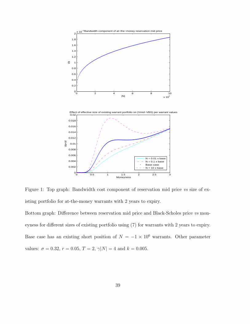
Figure 1 shows how V mid−V BS varies with moneyness and the size of the issuer’s
portfolio. Note that since the non-linearity with respect to |N | arises solely from
the lifetime cost component, which depends on the size of the warrant’s Gamma,
the effects are concentrated close-to-the-money. For in-the-money asset prices the
cost terms proportional to the size of the warrant’s Delta, which do not depend
on portfolio size, are more important, so the sensitivity of mid prices and bid-ask
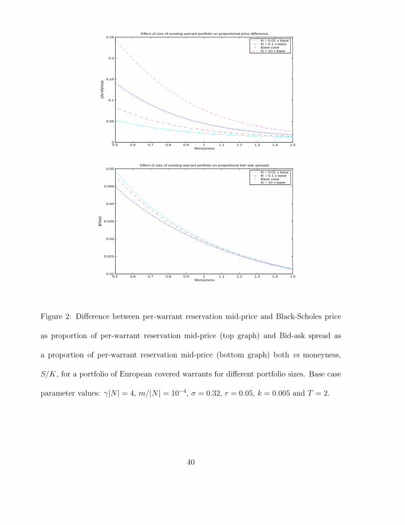
spreads to the size of the issuer’s existing holding is small. Figure 2 shows the effect
of the size of the issuer’s existing portfolio, |N |, on the proportional price difference
(top graph) and proportional bid-ask spread (bottom graph).
Insert Figure 1 here
Insert Figure 2 here
A number of difficulties arise in testing implications of the model in practice.
Empirical studies compare actual covered warrant and traded option prices rather
than reservation covered warrant and perfect market values. Obtaining data on
23
covered warrant issuers’ holdings is likely to be difficult, so it may only be possible
to obtain indirect support for some implications. Finally, since the theoretical results
are obtained holding all else constant it is important to include appropriate controls
in empirical tests.
However, the implications, that, because of the larger (short) positions and lower
quote depths, warrant prices should be greater and warrant bid-ask spreads smaller
than those of equivalent traded options, are exactly what was found by Bartram
& Fehle (2004) for both relative prices and bid-ask spreads in German markets.
Whilst not a direct test of sensitivity to portfolio size, this is consistent with the
model’s implications. Higher prices for covered warrants than equivalent traded
options have also been found by Chan & Pinder (2000), Horst & Veld (2003) and
Abad & Nieto (2007) in Australian, Dutch and Spanish markets.
Abad & Nieto (2007) regress the relative price difference between warrant and
option markets on the ratio of the bid-ask spreads, amongst other characteristics.
They find warrants are more expensive when the warrant bid-ask spread just before
the transaction is smaller. They interpret the bid-ask spread ratio as a proxy for
the relative liquidity of the two markets. However, this is also consistent with the
effects of hedging costs: covered warrant issuers with larger portfolios (larger |N |)
have relatively higher mid-prices and also lower bid-ask spreads.
One potentially testable implication of the extent of the influence of hedging
cost issues on covered warrant prices22 is the predicted positive sensitivity of both
proportional and absolute bid-ask spreads to quote depth. This not been addressed
directly, however there is some indirect support. Bartram & Fehle (2004) find
22Other factors such as competition and adverse selection may also influence bid and ask prices.
24
minimum trade sizes are generally much smaller and proportional bid-ask spreads
are also significantly smaller for covered warrants than traded options. Bartram &
Fehle (2006) and Bartram, Fehle & Shrider (2007) also find statistically significantly
lower proportional bid-ask spreads for covered warrants.23 Finally Petrella (2006)
finds a significant positive relationship between the proportional bid ask spread and
the ‘reservation proportional bid-ask spread’, proportional to the tick-size ×m∆/V
where m is the number of assets underlying one warrant contract. This is consistent
with the costly hedging model, which predicts a larger quote depth m should be
associated with a larger proportional bid-ask spread.
4.2 Warrant characteristics
Corollary 3 The magnitude of the lifetime or bandwidth cost components of both
the reservation mid price and the reservation bid-ask spread increase with the war-
rant’s remaining life.
The bandwidth cost components V midb and Bb represent the effect of the costs of
following the hedging strategy during the lifetime of the warrant.24 Both increase
with time to maturity, as the longer the hedging strategy is followed, potentially
the more transactions and the greater the total cost.25
23Bartram & Fehle (2006) suggest the difference could be due to the greater depth offered by options
market-makers but do not control for depth in their regressions; Bartram, Fehle & Shrider (2007) argue
it is due to lower adverse selection in covered warrant markets. The implications of adverse selection and
issuer hedging costs for bid-ask spreads are similar and hence difficult to disentangle.24The hedging strategy involves keeping the number of the underlying asset within a band about the
warrant’s Delta. The width of the band is proportional to the absolute value of the Gamma.25Formally, this is because Lb(|Γ|) increases with time to maturity.
25
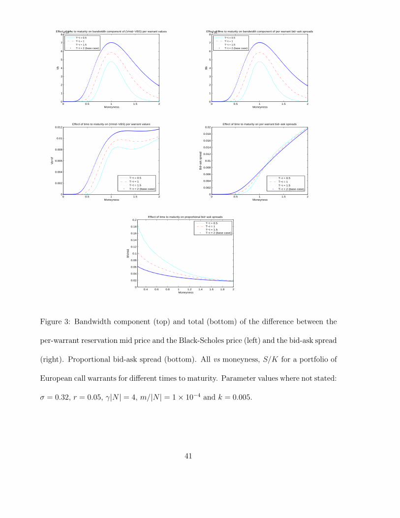
Insert Figure 3 here
The top graphs in Figure 3 show the effect is greatest for both V midb and Bb for
close to the money asset prices. This is because the bandwidth cost component is a
function of the warrant’s absolute Gamma integrated over the remaining life of the
warrant. A difficulty in testing for this is that the initial and final cost components
are both one-off costs and so do not increment with time to maturity. As shown
in the middle graphs in Figure 3, depending on the warrant’s moneyness, overall
bid-ask spreads or V mid − V BS can either increase or decrease with maturity, T . It
is thus important to control for moneyness, potentially via initial/final costs, or |∆|,
when testing for the positive dependence of either relative prices or bid-ask spreads
on time-to-maturity.
A number of studies support the predicted relationship between relative warrant
and option prices and time to maturity. Bartram & Fehle (2004) regress the ratio
of warrant to option ask prices (AR) on, amongst other characteristics, the corre-
sponding ratio of bid prices, time to maturity, moneyness, asset volatility and the
number of competing warrants. Once cross-sectional variation has been removed
they find a positive relationship between the ask ratio and time to maturity. Sim-
ilarly Abad & Nieto (2007) find the relative price difference between warrant and
option prices is significantly positively related to time to maturity.
Most empirical studies of bid-ask spreads use the proportional rather than the
absolute bid-ask spread. The bottom graph in Figure 3 shows that, unlike the
absolute bid-ask spread, the proportional bid-ask spread decreases with time-to-
maturity, and by more, the lower the moneyness: moreover this result does not
require controls for |∆|.
26
A number of empirical studies in both option and covered warrant markets have
consistently found that proportional bid-ask spreads decrease with moneyness and
time to maturity.26 Kaul et al (2004), the only study on either covered warrant or
traded option spreads to use absolute bid-ask spread, showed empirically that whilst
average absolute bid-ask spreads increase across moneyness groupings, proportional
bid-ask spreads generally decrease across the same moneyness groups. His results
with respect to time-to-maturity were also broadly consistent with the theoretical
and numerical results in Corollary 3 and Figure 3.
4.3 Characteristics of the underlying asset market
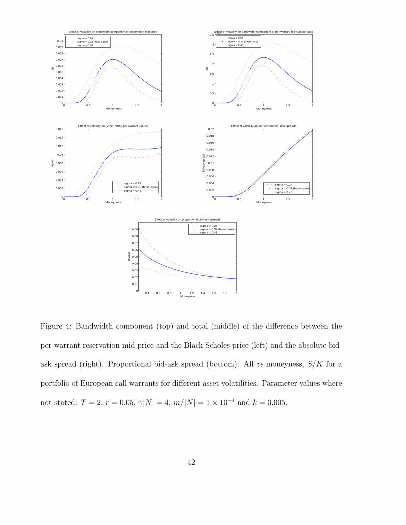
Insert Figure 4 here
Figure 4 shows the effect of asset volatility on the difference between the reser-
vation mid price and perfect market value and on the per-warrant bid-ask spread.
The bandwidth terms, in the top graphs, increase monotonically with asset volatil-
ity; however no unambiguous statement is possible for the combined terms, in the
middle graphs, as it depends on the relative sizes of the lifetime and initial/final
cost terms and also the moneyness. Thus, as for time to maturity, it is necessary to
control for e.g. the initial/final cost level S|∆| in testing for the positive relation-
ships between asset volatility and both absolute bid-ask spreads and the difference
26Cho & Engle (1999), Bartram & Fehle (2006) and Petrella (2006) all find significantly negative
coefficients in their regressions of proportional bid-ask spreads on moneyness. Jameson & Wilhelm (1992)
do not include moneyness but do include elasticity S∆/V , which is strictly decreasing in moneyness for
call warrants and find a significant negative coefficient. Similarly George & Longstaff (1993), Cho &
Engle (1999) and Petrella (2006) all find significantly negative coefficients for time-to-maturity.
27
between covered warrant and equivalent option prices. Moreover, the bottom graph
shows that proportional bid-ask spreads decrease with volatility: as with time to
maturity, warrant values increase more with volatility than absolute bid-ask spreads.
It is clear from the functional forms for V mid and B that both increase with the
underlying asset bid-ask spread, k.27 The effect is greater for the bandwidth cost
terms, which scale as k2/3, than the initial or final cost terms, which scale as k.
So whilst the relationship between asset bid-ask spread and both warrant bid-ask
spreads and the difference between covered warrant and equivalent exchange traded
option prices is positive, it should be strongest for close-to-the-money asset prices
and when transaction costs are small.
Corollary 4 The magnitude of the difference between the reservation mid price
and the perfect market price and the absolute and proportional reservation bid-ask
spreads all increase with the proportional bid-ask spread in the underlying asset
To date there is no empirical evidence on the relationship between either asset
volatility or bid-ask spread on the relative pricing of covered warrants and traded
options.28 In contrast, the general principle that dynamic hedging costs affect bid-
ask spreads in both covered warrant and traded option markets has relatively wide-
spread support. Cho & Engle (1999), Kaul et al (2004) and Petrella (2006) all
found that option or warrant proportional bid-ask spreads are significantly positively
related to a measure of the initial hedging costs kS∆. Proxies for rebalancing
27After some algebra we find this is also the case for the proportional bid-ask spread, B/V mid.28Whilst Bartram & Fehle (2004) include asset volatility in their regression of relative ask prices
on relative bid prices, since they also include asset dummies, they interpret the significantly negative
coefficient as evidence of lower sensitivity of warrants than options to changes in liquidity. .
28
costs have been considered explicitly for options markets by Jameson & Wilhelm
(1992) and Kaul et al (2004), and, for covered warrant markets, Petrella (2006). All
found the proxies to be positively and statistically significantly related to spreads.
Similarly, regressions which have included proxies for option or underlying asset
price risk as (a component) of explanatory variables29 have found results consistent
with a positive impact of asset price volatility on option spreads.
4.4 Summary
The warrant issuer costly hedging model has the following empirical implications.
Covered warrant prices are greater than those of equivalent traded options, whereas
covered warrant bid-ask spreads are smaller than those for equivalent traded op-
tions. The difference between covered warrant and equivalent traded option prices
increases with the size of the issuer’s existing portfolio (though at a decreasing rate)
and with the asset’s bid-ask spread and, controlling for moneyness, with the time
to maturity and asset volatility. Similarly both absolute and proportional bid-ask
spreads increase with quote depth and the asset’s bid-ask spread and decrease with
the size of the issuer’s existing portfolio. Holding moneyness constant, the absolute
bid-ask spread increases and the proportional bid-ask spread decreases with time to
maturity. The proportional bid-ask spread also decreases with moneyness.
5 Conclusion and further work
In this paper we developed a model for the reservation bid and ask prices of covered
warrants, taking into account hedging costs and a covered warrant issuer’s portfolio
29Jameson & Wilhelm (1992), Cho & Engle (1999), Petrella (2006)
29
composition and risk aversion. This provided a new supply-side explanation for
the empirically documented regularity that covered warrant prices are consistently
higher than those of equivalent exchange-traded options.
The existing empirical evidence on the relative pricing of covered warrants and
exchange traded options and on bid-ask spreads in options and warrant markets is
broadly supportive of the wider implications of the model. Further empirical work
needs to be done to investigate some novel implications of the model which have not
yet been addressed explicitly, e.g. the effects of the magnitude of a covered warrant
issuer’s overall portfolio on the relative overpricing of covered warrants.
The characteristics of covered warrant markets which drive the model are also
present in markets for many structured products offered to retail investors in recent
years:30 issuers are also market makers and hold net short positions. Interestingly,
similar findings about the relative pricing of structured products (that they are
greater than the price of equivalent exchange traded products, for both convex
and concave payoffs31) have been documented for a range of such products. The
supply-side cost argument in this paper may also give a partial explanation for this.
More generally, the model in section 3, extended to positive as well as negative N ,
can be viewed in the spirit of an inventory cost model for options market-makers32:
30See Stoimenov & Wilkens (2006) for a recent review.31See e.g. Burth, Kraus & Wohlwend (2001) for empirical evidence on a structured product with
a concave payoff. The dependence of the reservation mid price on the absolute value of the warrant’s
Gamma or Delta, combined with the sign of the (net) number of warrants held in the portfolio, means
the issuers of structured products (SPs), who generally have a net short position, will have a reservation
mid-price for any SP which is higher than the SP’s perfect market value (since sgn(N) = −1) irrespective
of the sign of the Gamma of a single long SP.32The model gives reservation prices, at which a market-maker would be indifferent between selling
30
inventory costs (i.e. the effect of the number of options held, N) are reflected in
reservation bid and ask prices indirectly through the optimal hedging bandwidth
and hence the residual risk the market-maker optimally incurs. Thus, as in inventory
cost models of underlying asset markets (e.g. Ho & Stoll (1981)), the mid-price is
negatively related to the inventory level (though for options this relationship is non-
linear), the bid-ask spread is positively related to the quote depth and both bid-ask
spread and mid price are positively related to the risk of the marginal (existing
portfolio) position. It would be interesting to explore this relationship further in
future work.
6 Appendix
Proof of Proposition 2
We have g(ΛQ|ΛP ) = G(ΛP + ΛQ) − G(ΛP ) + gi(|ΛQ|), where gi(|ΛQ|) =
−kS|QBSS | is the leading order initial cost of changing the number of the under-
lying asset held, and from Proposition 1
G(ΛP ) ≈ GBS(ΛP ) + Gb(|ΓP |) + Gf (|∆P |)
G(ΛP + ΛQ) ≈ GBS(ΛP + ΛQ) + Gb(|ΓP + ΓQ|) + Gf (|∆P + ∆Q|)
We can thus write g(ΛQ|ΛP ) ≈ gBS(ΛQ) + gb(ΛQ|ΛP ) + gf (ΛQ|ΛP ) + gi(ΛQ) where
gBS(ΛQ) ≡ GBS(ΛP +ΛQ)−GBS(ΛP ), gb(ΛQ|ΛP ) ≡ Gb(|ΓP +ΓQ|)−Gb(|Γ
P |) and
(ask price) or buying (bid price) the quoted number of options and hedging optimally, or not. Hence
it does not incorporate expected order flow or maximise the market-maker’s profit. It also does not
consider adverse selection issues. A fuller model is beyond the scope of this paper; however, we would
expect utility-maximising ask and bid prices to incorporate the same factors which underlie reservation
prices based on inventory considerations and to lie outside the reservation bid-ask spread.
31
gf (ΛQ|ΛP ) ≡ Gf (|∆P + ∆Q|) − Gf (|∆P |). gBS(ΛQ) is the Black-Scholes value of
the portfolio with payoff ΛQ since the Black-Scholes differential equation is linear.
gb(ΛQ|ΛP ) satisfies
LBS(gb(ΛQ|ΛP )) =
(
γ̂σ2S2
2
)
(
H∗2
P+Q − H∗2
0
)
−
(
γ̂σ2S2
2
)
(
H∗2
P − H∗2
0
)
=
(
γ̂σ2S2
2
)
(
H∗2
P+Q − H∗2
P
)
subject to gb(ΛQ|ΛP )(S, T ) = Gb(|ΓP + ΓQ|)(S, T ) − Gb(|Γ
P |)(S, T ) = 0 − 0 = 0,
where γ̂ ≡ γe−r(T−t) and H∗P+Q, H∗
P represent the semi-bandwidths associated
with payoffs ΛP + ΛQ and ΛP respectively and are given by H∗P+Q =
(
3kS2γ̂
) 1
3 |ΓP +
ΓQ + ξS2 |
2
3 and H∗P =
(
3kS2γ̂
) 1
3 |ΓP + ξS2 |
2
3 with ξ(t) = µ−rγ̂(t)σ2 . gf (ΛQ|ΛP ) satisfies
LBS(gf (ΛQ|ΛP )) = 0 subject to
gf (ΛQ|ΛP )(S, T ) = −k(|ξ(T ) − S(∆P (S, T ) + ∆Q(S, T ))| − |ξ(T )|)
+k(|ξ(T ) − S∆P (S, T )| − |ξ(T )|)
= −k(|ξ(T ) − S(∆P (S, T ) + ∆Q(S, T ))| − |ξ(T ) − S∆P (S, T )|)
If P and Q represent portfolios of a single European covered warrant, so ΛP =
NΛV , ΛQ = nΛV , let V BS(S, t) be the Black-Scholes value of a single long warrant
with payoff ΛV at maturity T and ∆(S, t), Γ(S, t) be the Black-Scholes Delta and
Gamma of the single long warrant respectively. Then the Black-Scholes values of the
portfolios’ Deltas and Gammas are given by ∆P = N∆, ∆Q = n∆, ΓP = NΓ and
ΓQ = nΓ. Writing also g(nΛV |NΛV ) ≡ g(n|N) ≈ nV BS +gb(n|N)+gf (n|N)+gi(n)
we find gBS(ΛQ) = nV BS , gi(n) = −k|n|S|∆(S, T )|, gb(n|N) satisfies
LBS(gb(n|N)) =
(
γ̂σ2
2
)
(
3k
2γ̂
)2
3(
|(N + n)S2Γ + ξ|4
3 − |NS2Γ + ξ|4
3
)
32
subject to gb(n|N)(S, T ) = 0. Assuming |NS2Γ + ξ| � |nS2Γ| this becomes
LBS(gb(n|N)) =
(
γ̂σ2
2
)
(
3k
2γ̂
)2
3
|NS2Γ + ξ|4
3
(
1 +nS2Γ
NS2Γ + ξ
) 4
3
− 1
≈
(
γ̂σ2
2
)
(
3k
2γ̂
)2
3
(
sgn[NS2Γ + ξ]4
3n(S2Γ)|NS2Γ + ξ|
1
3
+2
9n2(S2Γ)2|NS2Γ + ξ|−
2
3
)
and gf (n|N) satisfies LBS(gf (n|N)) = 0 with final condition, assuming sgn[ξ(T ) −
(N + n)S∆(S, T )] = sgn[ξ(T ) − NS∆(S, T )] = −sgn[N ]sgn[∆]
gf (n|N)(S, T ) = −k(|ξ(T ) − (N + n)S∆(S, T )| − |ξ(T ) − NS∆(S, T )|)
= −k sgn[ξ(T ) − (N + n)S∆(S, T )] (−nS∆(S, T ))
= −sgn[N ] knS|∆(S, T )|
The bid price is defined as V bid(m|N) = g(m|N)/m with m > 0, so setting
n = +m and writing V bid(m|N) ≈ V BS + V bidb (m|N) + V bid
f (m|N) + V bidi (m) we
find
LBS(V bidb (m|N)) ≈
(
γ̂σ2
2
)
(
3k
2γ̂
)2
3
(
sgn[NS2Γ + ξ]4
3(S2Γ)|NS2Γ + ξ|
1
3
+2
9m(S2Γ)2|NS2Γ + ξ|−
2
3
)
s.t. V bidb (m|N)(S, T ) = 0 and LBS(V bid
f (m|N)) = 0 s.t. V bidf (m|N)(S, T ) =
−ksgn[N ]S|∆(S, T )|. V bidi (m) = −kS|∆(S, T )|.
Similarly the ask price is defined as V ask(m|N) = −g(−m|N)/m with m > 0, so
setting n = −m and writing V ask(m|N) ≈ V BS+V askb (m|N)+V ask
f (m|N)+V aski (m)
we find
LBS(V askb (m|N)) ≈
(
γ̂σ2
2
)
(
3k
2γ̂
)2
3
(
sgn[NS2Γ + ξ]4
3(S2Γ)|NS2Γ + ξ|
1
3
−2
9m(S2Γ)2|NS2Γ + ξ|−
2
3
)
33
s.t. V askb (m|N)(S, T ) = 0 and LBS(V ask
f (m|N)) = 0 s.t. V askf (m|N)(S, T ) =
−ksgn[N ]S|∆(S, T )| so V askf = V bid
f . However V aski (m) = −k |−m|
(−m)S|∆(S, t)| =
+kS|∆(S, t)| so V aski = −V bid
i .
Finally, since all the differential equations are linear, V mid(m|N) = V bid(m|N)+V ask(m|N)2
can be represented by V mid(m|N) ≈ V BS + V midb (m|N) + V mid
f (m|N) + V midi (m),
where V midb (m|N) satisfies
LBS(V midb (m|N)) ≈
(
γ̂σ2
2
)
(
3k
2γ̂
)2
3
sgn[NS2Γ + ξ]4
3(S2Γ)|NS2Γ + ξ|
1
3 (13)
s.t. V mid(m|N)(S, T ) = 0. If NS2Γ � ξ then, recalling Γ > 0 for vanilla options,
this can be further simplified to
LBS(V midb (m|N)) ≈
(
γ̂σ2
2
)
(
3k
2γ̂
)2
3
sgn[N ]4
3|N |
1
3 |S2Γ|4
3
s.t. V mid(m|N)(S, T ) = 0, which is equivalent to V mid(m|N) = −sgn[N ]43k2
3 |N |1
3 Lb(|Γ|)
with Lb satisfying
LBS(Lb) = −
(
γ̂σ2S2
2
)
(
3S
2γ̂
)2
3
|Γ|4
3 (14)
s.t. Lb(S, T ) = 0. Numerical simulations using (13) confirm our results are not
sensitive to the inclusion of ξ. V midf (m|N) satisfies LBS(V mid
f (m|N)) = 0 s.t.
V midf (m|N)(S, T ) = −ksgn[N ]S|∆(S, T )| and if ∆(S, T ) is one-signed, as is the case
for long call warrant then V midf (S, t) = −ksgn[N ]S|∆(S, t)|. However V ask
i = −V bidi
so V midi = 0.
Similarly B(m|N) = V ask(m|N)−V bid(m|N) can be represented by B(m|N) ≈
Bb(m|N) + Bf (m|N) + Bi(m), where Bb(m|N) satisfies
LBS(Bb(m|N)) ≈ −
(
γ̂σ2
2
)
(
3k
2γ̂
)2
3 4
9m(S2Γ)2|NS2Γ + ξ|−
2
3
34
s.t. Bb(m|N)(S, T ) = 0. Again, if NS2Γ � ξ then this can be further simplified to
LBS(Bb(m|N)) ≈ −4
9m|N |−
2
3
(
γ̂σ2
2
)
(
3k
2γ̂
)2
3
|S2Γ|4
3
s.t. V mid(m|N)(S, T ) = 0, which is equivalent to Bb(m|N) = 49m|N |−
2
3 k2
3 Lb(|Γ|)
with Lb satisfying (14), V askf = V bid
f so Bf = 0 and Bi(m) = 2kS|∆(S, t)|.
Sketch of Proof of Corollary 1
It is immediate from (7), noting Lb(|Γ|) > 0 and N < 0, that V mid(m|N) −
V BS > 0. Similarly from (9), B(m|N) > 0. Hence clearly V ask(m|N) = V mid(m|N)+
12B(m|N) > V BS , and
V bid(m|N) = V mid(m|N)−1
2B(m|N) = V BS+
4
4|N |
1
3 k2
3 Lb(|Γ|)
(
1 −m
6|N |
)
> V BS
since m/|N | � 1 by assumption.
Sketch of Proof of Corollary 2
Differentiating (7) and (9) w.r.t. |N | gives ∂(V mid(m|N)−V BS)∂|N | = ∂V mid(m|N)
∂|N | ≈
49 |N |
−2
3 k2
3 Lb(|Γ|) > 0; ∂B(m|N)∂|N | ≈ − 8
27m|N |−5
3 k2
3 Lb(|Γ|) < 0 ⇒∂(
B
V mid
)
∂|N | ≈ 1V mid
∂B∂|N |−
B(V mid)2
∂V mid
∂|N | < 0.
Differentiating (7) and (9) w.r.t. m gives ∂(V mid(m|N)−V BS)∂m = 0; ∂B(m|N)
∂m ≈
49 |N |−
2
3 k2
3 Lb(|Γ|) > 0 ⇒∂(
B
V mid
)
∂m ≈ 1V mid
∂B∂m − B
(V mid)2∂V mid
∂m > 0.
Sketch of Proof of Corollary 3
V midb and Bb depend on time to maturity only through Lb(|Γ|), which increases
with time to maturity since γ̂(t)σ2S2
2
(
3S2γ̂(t)
) 2
3 |Γ(S, t)|4
3 > 0∀(S, t).
Sketch of Proof of Corollary 4
Differentiating (7) and (9) w.r.t. k gives ∂(V mid(m|N)−V BS)∂k ≈ 8
9 |N |1
3 k− 1
3 Lb(|Γ|)+
S|∆| > 0; ∂B(m|N)∂k ≈ 8
27m|N |−2
3 k− 1
3 Lb(|Γ|) + 2S|∆| > 0 and
∂(
B
V mid
)
∂k ≈V BS
(
8
27m|N |−
2
3 k−
1
3 Lb(|Γ|)+2S|∆|
)
+ 20
27|N |
1
3 k2
3 Lb(|Γ|)S|∆|
(V mid)2> 0
35
References
[1] Abad, D and B Nieto (2007) The Unavoidable Task of Understanding Warrants
Pricing. Working paper
[2] Bartram, SM and F Fehle (2004) Alternative Market Structures for Derivatives.
Working paper
[3] Bartram, SM and F Fehle (2006) Competition without Fungibility: Evidence
from Alternative Market Structures for Derivatives. Journal of Banking and
Finance 31, 659-677
[4] Bartram, SM, Fehle, F and D Shrider (2007) Does Adverse Selection Affect
Bid-Ask Spreads for Options? Working paper
[5] Burth, S, Kraus, T and H Wohlwend (2001) The Pricing of Structured Products
in the Swiss Market. Working paper
[6] Chan, HW and SM Pinder (2000) The value of liquidity: Evidence from the
derivatives market. Pacific-Basin Finance Journal 8, 483-503
[7] Cho, Y and R Engle (1999) Modeling the impacts of market activity on bid-ask
spreads in the option market NBER Working Paper 7331
[8] Clewlow, L and S.D. Hodges (1997) Optimal delta-hedging under transaction
costs Journal of Economic Dynamics and Control 21, 1353-1376
[9] Damgaard, A (2003) Utility based option evaluation with proportional trans-
action costs. Journal of Economic Dynamics and Control 27, 667-700
[10] Davis, MHA, V.G. Panas and T. Zariphopoulou (1993) European option pricing
with transaction costs. SIAM Journal of Control and Optimisation 31, 470-493
36
[11] George, T and F Longstaff (1993) ‘Bid-Ask Spreads and Trading Activity in
the S&P100 Index warrants Market. Journal of Financial and Quantitative
Analysis 28, 381-397
[12] Goldman Sachs (2007) Base prospectus: Programme for the Issuance of War-
rants and Certificates 26 March, 2007
[13] Ho, T and HR Stoll (1981) Optimal dealer pricing under transactions and
return uncertainty. Journal of Financial Economics 9, 47-73
[14] Hodges, SD and A. Neuberger (1989) Optimal replication of contingent claims
under transaction costs. Review of Futures Markets 8, 222-239
[15] Horst, J and C Veld (2003) Behavioral Preferences for Individual Securities:
The Case for Call Warrants and Call options. Working paper
[16] Jameson, M and W Wilhelm (1992) Market making in the options markets and
the costs of discrete hedge rebalancing. Journal of Finance 47, 765-779
[17] Kaul, G, Nimalendran, M and D Zhang (2004) Informed trading and option
spreads. Working paper
[18] Petrella, G (2006) Option bid-ask spread and scalping risk: Evidence from a
covered warrants market. Journal of Futures Markets 26, 843-867
[19] Rogers, LCH (2000) Why is the effect of proportional transaction costs O(δ2/3)?
Working paper
[20] Stoimenov, and Wilkens (2006) Are structured products fairly priced? An anal-
ysis of the German market for equity-linked instruments. Journal of Banking
and Finance 29, 2971-2993
37
[21] Whalley, AE (1998) Option pricing with transaction costs. D. Phil. thesis,
Oxford University
[22] Whalley, AE and P. Wilmott (1997) An asymptotic analysis of the Davis, Panas
& Zariphopoulou model for option pricing with transaction costs. Mathematical
Finance 7, 307-324
[23] Whalley, AE and P. Wilmott (1999) Optimal hedging of options with small but
arbitrary transaction cost structure. European Journal of Applied Mathematics
10, 117-139
[24] Zakamouline, VI (2006) European option pricing with both fixed and propor-
tional transaction costs. Journal of Economic Dynamics and Control 30, 1-25
38
0 2 4 6 8 10
x 105
0
0.2
0.4
0.6
0.8
1
1.2
1.4
1.6
1.8
2x 10
−3Bandwidth component of at−the−money reservation mid price
|N|
Vb
0 0.5 1 1.5 2 2.5 30
0.002
0.004
0.006
0.008
0.01
0.012
0.014
0.016
0.018
0.02Effect of effective size of existing warrant portfolio on (Vmid−VBS) per warrant values
Moneyness
Vb+V
f
N = 0.01 x baseN = 0.1 x baseBase caseN = 10 x base
Figure 1: Top graph: Bandwidth cost component of reservation mid price vs size of ex-
isting portfolio for at-the-money warrants with 2 years to expiry.
Bottom graph: Difference between reservation mid price and Black-Scholes price vs mon-
eyness for different sizes of existing portfolio using (7) for warrants with 2 years to expiry.
Base case has an existing short position of N = −1 × 10⁶ warrants. Other parameter
values: σ = 0.32, r = 0.05, T = 2, γ|N | = 4 and k = 0.005.
39
0.5 0.6 0.7 0.8 0.9 1 1.1 1.2 1.3 1.4 1.50
0.05
0.1
0.15
0.2
0.25Effect of size of existing warrant portfolio on proportional price difference
Moneyness
(Vb+
Vf)/V
mid
N = 0.01 x baseN = 0.1 x baseBase caseN = 10 x base
0.5 0.6 0.7 0.8 0.9 1 1.1 1.2 1.3 1.4 1.50.02
0.025
0.03
0.035
0.04
0.045
0.05Effect of size of existing warrant portfolio on proportional bid−ask spreads
Moneyness
B/Vm
id
N = 0.01 x baseN = 0.1 x baseBase caseN = 10 x base
Figure 2: Difference between per-warrant reservation mid-price and Black-Scholes price
as proportion of per-warrant reservation mid-price (top graph) and Bid-ask spread as
a proportion of per-warrant reservation mid-price (bottom graph) both vs moneyness,
S/K, for a portfolio of European covered warrants for different portfolio sizes. Base case
parameter values: γ|N | = 4, m/|N | = 10−4, σ = 0.32, r = 0.05, k = 0.005 and T = 2.
40
0 0.5 1 1.5 20
1
2
3
4
5
6
7
8x 10
−3Effect of time to maturity on bandwidth component of (Vmid−VBS) per warrant values
Moneyness
Vb
T−t = 0.5
T−t = 1
T−t = 1.5
T−t = 2 (base case)
0 0.5 1 1.5 20
0.002
0.004
0.006
0.008
0.01
0.012Effect of time to maturity on (Vmid−VBS) per warrant values
Moneyness
Vb+
Vf
T−t = 0.5T−t = 1T−t = 1.5T−t = 2 (base case)
0 0.5 1 1.5 20
1
2
3
4
5
6
7
8x 10
−3Effect of time to maturity on bandwidth component of per warrant bid−ask spreads
Moneyness
Bb
T−t = 0.5
T−t = 1
T−t = 1.5
T−t = 2 (base case)
0 0.5 1 1.5 20
0.002
0.004
0.006
0.008
0.01
0.012
0.014
0.016
0.018
0.02Effect of time to maturity on per warrant bid−ask spreads
MoneynessB
id−a
sk s
prea
d
T−t = 0.5T−t = 1T−t = 1.5T−t = 2 (base case)
0.4 0.6 0.8 1 1.2 1.4 1.6 1.8 20
0.02
0.04
0.06
0.08
0.1
0.12
0.14
0.16
0.18
0.2Effect of time to maturity on proportional bid−ask spreads
Moneyness
B/V
mid
T−t = 0.5T−t = 1T−t = 1.5T−t = 2 (base case)
Figure 3: Bandwidth component (top) and total (bottom) of the difference between the
per-warrant reservation mid price and the Black-Scholes price (left) and the bid-ask spread
(right). Proportional bid-ask spread (bottom). All vs moneyness, S/K for a portfolio of
European call warrants for different times to maturity. Parameter values where not stated:
σ = 0.32, r = 0.05, γ|N | = 4, m/|N | = 1 × 10⁻⁴ and k = 0.005.
41
0 0.5 1 1.5 20
0.001
0.002
0.003
0.004
0.005
0.006
0.007
0.008
0.009
0.01
Effect of volatility on bandwidth component of reservation mid price
Moneyness
Vb
sigma = 0.24
sigma = 0.32 (base case)
sigma = 0.48
0 0.5 1 1.5 20
0.002
0.004
0.006
0.008
0.01
0.012
0.014
0.016Effect of volatility on (Vmid−VBS) per warrant values
Moneyness
Vb+
Vf
sigma = 0.24sigma = 0.32 (base case)sigma = 0.48
0 0.5 1 1.5 20
0.5
1
1.5
2
2.5
3
3.5x 10
−7Effect of volatility on bandwidth component of per warrant bid−ask spreads
Moneyness
Bb
sigma = 0.24
sigma = 0.32 (base case)
sigma = 0.48
0 0.5 1 1.5 20
0.002
0.004
0.006
0.008
0.01
0.012
0.014
0.016
0.018
0.02Effect of volatility on per warrant bid−ask spreads
MoneynessB
id−a
sk s
prea
d
sigma = 0.24sigma = 0.32 (base case)sigma = 0.48
0.4 0.6 0.8 1 1.2 1.4 1.6 1.8 20
0.01
0.02
0.03
0.04
0.05
0.06
0.07
0.08
0.09
Effect of volatility on proportional bid−ask spreads
Moneyness
B/V
mid
sigma = 0.24sigma = 0.32 (base case)sigma = 0.48
Figure 4: Bandwidth component (top) and total (middle) of the difference between the
per-warrant reservation mid price and the Black-Scholes price (left) and the absolute bid-
ask spread (right). Proportional bid-ask spread (bottom). All vs moneyness, S/K for a
portfolio of European call warrants for different asset volatilities. Parameter values where
not stated: T = 2, r = 0.05, γ|N | = 4, m/|N | = 1 × 10⁻⁴ and k = 0.005.
42