Copyright by Vatsal Nilesh Shah 2020
250
Copyright by Vatsal Nilesh Shah 2020
Transcript of Copyright by Vatsal Nilesh Shah 2020

Copyright
by
Vatsal Nilesh Shah
2020

The Dissertation Committee for Vatsal Nilesh Shahcertifies that this is the approved version of the following dissertation:
On Variants of Stochastic Gradient Descent
Committee:
Sujay Sanghavi, Supervisor
Constantine Caramanis
Sanjay Shakkottai
Aryan Mokhtari
Anastasios Kyrillidis
On Variants of Stochastic Gradient Descent
by
Vatsal Nilesh Shah
DISSERTATION
Presented to the Faculty of the Graduate School of
The University of Texas at Austin
in Partial Fulfillment
of the Requirements
for the Degree of
DOCTOR OF PHILOSOPHY
THE UNIVERSITY OF TEXAS AT AUSTIN
August 2020

Dedicated to Mummy, Papa and Dada
In loving memory of Dadi

Acknowledgments
As I embarked upon the journey to pursue PhD from the familiar sur-
roundings of Mumbai to a new country and a new city with almost no ac-
quaintances, I was quite skeptical about whether it was the right choice. The
future is scary, but you can’t just run back to the past because it’s familiar 1.
While this quote provided me with a temporary respite during the unfamiliar,
uncomfortable start at UT, I have come to not only enjoy my time here but
also grown as a person and a researcher. None of this would have been possi-
ble without the never-ending support of my family, friends, collaborators, and
colleagues.
Prof. Sujay Sanghavi has been an amazing advisor who has provided
me with the right mix of guidance and independence during the course of my
PhD. Sujay’s unique analytical approach to problem-solving, ability to always
ask the right questions, focusing on the bigger picture while ensuring rigor in
theoretical guarantees are some of the many many things that have immensely
helped me during the course of my PhD. My PhD journey has had its fair share
of ups and downs and I would like to especially thank Sujay for always making
a point to talk about both my academic as well as personal well-being.
Without the constant guidance, support, and encouragement provided
1From How I Met Your Mother, Season 6 Episode 24: Challenge Accepted
v

by Prof. Anastasios Kyrillidis (Tasos), my thesis would have been non-existent.
I first met Tasos when he was a post-doc at UT and I feel incredibly lucky that
Sujay paired us to work together. He has been an amazing mentor, friend, and
collaborator ever since. I am indebted to him for his immense influence on my
writing style, critical thinking, time management, multi-tasking and so much
more.
I have taken two classes under Prof. Sanjay Shakkottai and the en-
thusiasm he shows in both teaching and research inevitably rubs off onto you.
Sanjay’s easy approachablility and expertise in a wide variety of fields implies
that I have had numerous discussions about different research topics in the cor-
ridors of EER and UTA. Prof. Constantine Caramanis’ structured approach
to both research and teaching means that there are numerous insights to be
gained in every discussion I have had with him. I also enjoyed interacting with
Constantine outside the academic environment especially at WNCG socials.
Prof. Aryan Mokhtari has been an exciting addition to WNCG and his exper-
tise in optimization has allowed me to discuss various research problems with
him which has contributed invaluably to my research.
I would like to thank all my collaborators for their invaluable contri-
butions to my thesis. During the course of our collaborations, I have really
admired the numerous insights I have gained via technical discussions with
Xiaoxia (Shirley) Wu, Soumya Basu, Erik Lindgren, Yanyao Shen, Ashish
Katiyar, John Chen, and Megasthenis Asteris. Shirley, in particular, has been
an inspiration to collaborate with due to her work ethic and ability to find
vi

a way to prove even the most challenging problems I have run into. I have
also learned tremendously while collaborating with Prof. Alex Dimakis, Prof.
Adam Klivans, and Prof. Rachel Ward. The numerous discussions I had
with students from Sujay’s lab group: Shanshan, Srinadh, Dohyung, Yanyao,
Ashish, Shuo, Anish, and Rudrajit have been quite instrumental towards the
completion of my thesis.
My three internships at Technicolor Research, Amazon, and Amazon
Web Services (AWS) have broadened my horizons and provided a diverse
glimpse of life in industry. I would like to thank my mentors at Technicolor,
Nikhil Rao, and Weicong Ding for the countless discussions and invaluable
guidance towards my first project in recommender systems. At Amazon, I
had the opportunity to work with a project in production for the Homepage
Personalization team. Ali Jalali’s mentorship was pivotal in helping me navi-
gate a steep learning curve that came with handling extremely large datasets.
At AWS, I had the opportunity to work under Anima Anandkumar, where
I had the learned about deep learning and computer vision, which came in
handy in the latter part of my thesis. During the course of these internships, I
had the amazing opportunity to have technical and non-technical discussions
with Farhad, Julian, Tan, Rushil, Teja, Shijia, Shaozhe, Kamyar, Michael,
Jeremy, Ben, Fanny, Thom, Yifan and many others.
I would also like to thank Karen, Melanie, Melody, Barry, Jaymie,
and Apipol for helping me resolve all the academic formalities with minimal
hassles. The efforts by Karen, Jaymie, and Apipol, in particular, have played
vii

an important part in fostering a sense of togetherness in WNCG by organizing
socials, potlucks, happy hours, and numerous other events.
The last six years at UT have been incredible thanks to some amazing
people I met in WNCG. Talking with Avradeep is like reading an encyclope-
dia; you will always get something new out of the conversation despite the
utility. Murat, thanks for being an amazing friend and more importantly in-
troducing me to the world of coffee shops, I don’t think I would have finished
my PhD without them. Shalmali has always played the role of a caring albeit
nosy guardian in WNCG and has been a source of inspiration throughout my
time here. I am thankful to Eirini for providing an incredible support system
both within and outside the walls of WNCG during some of my most difficult
moments. Soumya is always up for spontaneous plans from going to coffee
shops to live music events to taking last-minute road trips. My conversations
with him, about life, research, and everything else, have been fun, insightful,
and kept me grounded.
In the last three years, Ashish has helped me navigate all the ups
and downs in my life with utmost patience. I have had so many profound
conversations with him during our road trips, coffee shops, food trucks, Tous
Les Jours detours, and everything else. Monica has introduced me to climbing,
exotic food trucks, Colombian delicacies, and often provided the best advice
to all my problems. Oddwood Ales was definitely a start of an exciting series
of nights with Ashish, Manan, Monica and Soumya and I am hoping that the
tradition keeps on continuing albeit with more positive updates. Watching
viii

Champions League matches with Ajil and Manan, especially the legendary
Liverpool comeback against Barcelona, is something I will never forget. I
enjoyed hanging out with Mridula, Rajat, Ajil, Natasa, Erik, Sara, Derya,
Abhishek, Alan, Dave, Megha, amongst others in EER, at coffee shops, pubs,
dinners and over wine and trivia nights. I feel lucky to have met Divya,
Suriya, Ankit, Ethan, Karthikeyan, Avhishek who have all provided me with
invaluable guidance during my first few years at UT.
I would also like to thank my therapist Anita Stoll who has played a
significant role in helping me deal with trauma and the subsequent anxiety
during the course of my PhD. I have seen that graduate school can be a
pretty isolated environment especially for international students. In such cases,
asking for help is never easy and it took me a long time to recognize that.
There was also the initial skepticism about whether therapy is for me or the
usefulness of it, however I can confidently say that the benefits have heavily
outweighed the initial struggle. Since I started regular sessions with Anita, I
have been better equipped to deal with life and PhD.
In this terrifying world, all we have are the connections that we make2.
And I feel incredibly lucky to have met so many wonderful people during the
last six years. Pranav has been an amazing friend and I don’t think anything
I say here comes remotely close to doing justice to how much he has helped
me navigate the ups and downs of PhD life. It all started with random walks
2From Bojack Horseman: Season 3 Episode 4: Fish Out of Water
ix

and petty squabbles with Priyanka the chief-event planner, and with time
our friendship has continued to blossom over long talks, dinners, board game
nights, road trips and eventful bike rides. I hate Nitin for all the board games
he has won and all the keys he has ‘lost ’, but admire his kindhearted nature
along with his discipline and dedication in literally all his other endeavors. I
have admired Esha right from our first meeting∗ for her ambition, opinions,
providing the best sounding board for all my problems as well as bringing
much needed drama to my mundane life. Quarantining in 2020 would have
been way harder without Esha and Pranav’s improvised theatrics. I always
enjoyed having ambivalent conversations with Vikas.
Amongst my roommates, I have learned a lot from Venky (now Prof.
Venktesh) who also gets the title of nicest person to exist. I have grown
tremendously as a person just by observing how he conducts himself in diffi-
cult situations. I will always cherish the fun conversations, cooking escapades
and Netflix binging sessions with Bharath and I am grateful to him for taking
care of me through the toughest phase of my life. Long conversations and
countless road trips perfectly encapsulate my happening friendship with De-
vesh. Recreating the road trip through Spain in Zindagi Na Milegi Dobara
with Devesh and Venky remains a highlight of grad school.
I had a lot of fun with Surbhi during our late-night work sessions at cof-
fee shops, exploring tea places, dinners and board games primarily due to her
relentless energy and enthusiasm. In the last couple of years, I have enjoyed all
the spontaneous and non-spontaneous plans with Akanksha from long talks,
x

working at coffee shops, to dinners and board games. I had a lot of fun talk-
ing about life, Mumbai and life in Mumbai amongst many other things with
Prerana. It was quite memorable hanging out with Aastha, Kartik, Mad-
humitha, Manan, Nihal, Nithin over dinners, badminton, trivia nights, etc.
I will also cherish my countless interactions with Ankith, Anudhyan, Arjun,
Arun, Bhavin, Brinda, Eddy, Luca, Parshu, Pooja, Preeti, Priya, Roshan,
Shounak, Siddharth, and numerous other people who I have missed out on.
Akshay has been one of my closest confidantes for over 11 years as he
has helped me every step of the way during my PhD. In fact, without him, I
may not have begun this wonderful journey at UT. Long conversations with
Yatish and Sneha along with impromptu dinner plans, trips, and travelling
were a particular highlight of my Fall semester in the Bay area. Deeksha has
not only been a great friend but also an inspiration in how she continues to
have a social impact while pursuing her PhD. I have come to realize that I am
not that great at keeping in touch with long-distance friends and I would like
to thank Aakash, Adarsh, Ankush, Gurbaksh, Hiteshi, Jay, Jainik, Siddharth,
Tejas(es), Udit, Vidhya, Vivek and Yashasvi who have kept in touch with me
over the years.
I would like to thank Prof. Karandikar, who was my undergraduate
advisor, for igniting my interest in the field of optimization. Prof. Borkar
played an instrumental role in convincing me to pursue PhD at UT Austin
and is always a delight to talk with regarding both academic and non-academic
endeavors. I still cherish the publication of my first few papers with Prof. B.
xi

K. Mohan and Surendar Verma which ultimately provided an early motivation
in pursuing graduate school.
I feel extremely lucky to be blessed with the unconditional, unwavering
love, support and encouragement by my parents. Without their countless
sacrifices, hardships and struggles, none of this would have been possible. They
have supported me every step of the way on this journey and always allowed
me to express myself and I am really thankful for that. One of the last vivid
memory I have of my late grandmother Indira dadi is that when I was having
second thoughts about pursuing grad school, she was the one who provided
the final push that finally convinced me and there was no looking back after
that. I know that she would have been proud of what I have accomplished
and the person I have become in the last 6 years. Much to the annoyance
of my parents, my grandfather has always been my biggest defender and I
always enjoy goofing around with him at home, on video calls and during
trips. I would also like to thank Prakash fua, Sangeeta fai, Vrajesh mama,
Pinki mami, Paresh kaka, Smita kaki and Manju ba who have constantly
supported me throughout this journey. Special shoutout to my cousins Aarya,
Ashit jiju, Binita didi, Ishita, Utsav, Urvi (aka Urvashi), and for ensuring that
my India trips are always filled with memorable stories and adventures.
No matter how you get there or where you end up, human beings have
this miraculous gift to make that place home3. When I first came to Austin,
the weather was too hot and the food portions too big and everything miles
3From The Office (U.S.), Season 9 Episode 25: Finale
xii

apart. However, as time passed by, I have come around to enjoy the same
things which annoyed me at first. Austin has just been like a home away from
home and I will truly miss this stupid, wonderful, crazy, exciting city.
xiii

On Variants of Stochastic Gradient Descent
Vatsal Nilesh Shah, Ph.D.
The University of Texas at Austin, 2020
Supervisor: Sujay Sanghavi
Stochastic Gradient Descent (SGD) has played a crucial role in the suc-
cess of modern machine learning methods. The popularity of SGD arises due
to its ease of implementation, low memory and computational requirements,
and applicability to a wide variety of optimization problems. However, SGD
suffers from numerous issues; chief amongst them are high variance, slow rate
of convergence, poor generalization, non-robustness to outliers, and poor per-
formance for imbalanced classification. In this thesis, we propose variants of
stochastic gradient descent, to tackle one or more of these issues for different
problem settings.
In the first chapter, we analyze the trade-off between variance and
complexity to improve the convergence rate of SGD. A common alternative
in the literature to SGD is Stochastic Variance Reduced Gradient (SVRG),
which achieves linear convergence. However, SVRG involves the computation
of a full gradient every few epochs, which is often intractable. We propose the
Cheap Stochastic Variance Reduced Gradient (CheapSVRG) algorithm that
xiv
attains linear convergence up to a neighborhood around the optimum without
requiring a full gradient computation step.
In the second chapter, we aim to compare the generalization capa-
bilities of adaptive and non-adaptive methods for over-parameterized linear
regression. Of the many possible solutions, SGD tends to gravitate towards
the solution with minimum `2-norm while adaptive methods do not. We pro-
vide specific conditions on the pre-conditioner matrices under which a subclass
of adaptive methods has the same generalization guarantees as SGD for over-
parameterized linear regression. With synthetic examples and real data, we
show that minimum norm solutions are not an excellent certificate to guarantee
better generalization.
In the third chapter, we propose a simple variant of SGD that guar-
antees robustness. Instead of considering SGD with one sample, we take a
mini-batch and choose the sample with the lowest loss. For the noiseless
framework with and without outliers, we provide conditions for the conver-
gence of MKL-SGD to a provably better solution than SGD in the worst case.
We also perform the standard rate of convergence analysis for both noiseless
and noisy settings.
In the final chapter, we tackle the challenges introduced by imbalanced
class distribution in SGD. In place of using all the samples to update the
parameter, our proposed Balancing SGD (B-SGD) algorithm rejects samples
with low loss as they are redundant and do not play a role in determining the
separating hyperplane. Imposing this label-dependent loss-based thresholding
xv

scheme on incoming samples allows us to improve the rate of convergence and
achieve better generalization.
xvi

Table of Contents
Acknowledgments v
Abstract xiv
List of Tables xxii
List of Figures xxv
Chapter 1. Introduction 1
1.1 Contributions and Organization . . . . . . . . . . . . . . . . 2
1.2 Chapter 2: Trading-off Variance and Complexity in StochasticGradient Descent . . . . . . . . . . . . . . . . . . . . . . . . 3
1.3 Chapter 3: On the Generalization of Adaptive Methods forOver-parameterized Linear Regression . . . . . . . . . . . . 5
1.4 Chapter 4: Choosing the Sample with Lowest Loss makesSGD Robust . . . . . . . . . . . . . . . . . . . . . . . . . . . 6
1.5 Chapter 5: Balancing SGD: Faster Optimization for Imbal-anced Classification . . . . . . . . . . . . . . . . . . . . . . . 8
Chapter 2. Trading-off Variance and Complexity in StochasticGradient Descent 10
2.1 Introduction . . . . . . . . . . . . . . . . . . . . . . . . . . . 11
2.2 Related work . . . . . . . . . . . . . . . . . . . . . . . . . . 14
2.3 Our variance reduction scheme . . . . . . . . . . . . . . . . 16
2.4 Convergence analysis . . . . . . . . . . . . . . . . . . . . . . 19
2.4.1 Convergence Guarantees . . . . . . . . . . . . . . . . 21
2.5 Experiments . . . . . . . . . . . . . . . . . . . . . . . . . . . 23
2.5.1 Properties of CheapSVRG . . . . . . . . . . . . . . 23
2.5.2 `2-regularized logistic regression . . . . . . . . . . . . 29
2.6 Conclusions . . . . . . . . . . . . . . . . . . . . . . . . . . . 30
xvii
Chapter 3. On the Generalization of Adaptive Methods 33
3.1 Introduction . . . . . . . . . . . . . . . . . . . . . . . . . . . 34
3.2 Problem Setup . . . . . . . . . . . . . . . . . . . . . . . . . 38
3.2.1 Non-adaptive Methods in Under-parameterized Lin-ear Regression . . . . . . . . . . . . . . . . . . . . . 41
3.2.2 Adaptive Methods in Under-parameterized Linear Re-gression . . . . . . . . . . . . . . . . . . . . . . . . . 42
3.3 Over-parameterized linear regression . . . . . . . . . . . . . 43
3.3.1 Performance on Training Set for Non-Adaptive Methods 43
3.3.2 Performance on Training Set for Adaptive Methods . 44
3.4 Performance on Unseen Data . . . . . . . . . . . . . . . . . 46
3.4.1 Spectral Representation . . . . . . . . . . . . . . . . 46
3.4.2 Closed Form Expression for the Iterates . . . . . . . 47
3.4.3 `2-norm Regularized Linear Regression. . . . . . . . 49
3.4.4 Unregularized Linear Regression. . . . . . . . . . . . 50
3.5 Experiments . . . . . . . . . . . . . . . . . . . . . . . . . . . 54
3.5.1 Linear Regression . . . . . . . . . . . . . . . . . . . 55
3.5.1.1 Counter Example . . . . . . . . . . . . . . 56
3.5.2 Deep Learning . . . . . . . . . . . . . . . . . . . . . 61
3.5.2.1 Hyperparameter tuning . . . . . . . . . . . 68
3.5.2.2 Results . . . . . . . . . . . . . . . . . . . . 68
3.6 Conclusions and Future Work . . . . . . . . . . . . . . . . . 70
Chapter 4. Towards Improving the Robustness of SGD 72
4.1 Related Work . . . . . . . . . . . . . . . . . . . . . . . . . . 75
4.2 Problem Setup . . . . . . . . . . . . . . . . . . . . . . . . . 77
4.3 Understanding MKL-SGD . . . . . . . . . . . . . . . . . . . 80
4.3.1 Noiseless setting with no outliers . . . . . . . . . . . 81
4.3.2 Outlier setting . . . . . . . . . . . . . . . . . . . . . 82
4.4 Convergence Rates . . . . . . . . . . . . . . . . . . . . . . . 90
4.5 Experiments . . . . . . . . . . . . . . . . . . . . . . . . . . . 92
4.5.1 Linear Regression . . . . . . . . . . . . . . . . . . . 92
4.5.2 Neural Networks . . . . . . . . . . . . . . . . . . . . 92
xviii

4.6 Discussion and Future Work . . . . . . . . . . . . . . . . . . 95
4.7 Conclusion . . . . . . . . . . . . . . . . . . . . . . . . . . . . 97
Chapter 5. Balancing SGD: Faster Optimization for ImbalancedClassification 98
5.1 Introduction . . . . . . . . . . . . . . . . . . . . . . . . . . . 98
5.2 Related Work . . . . . . . . . . . . . . . . . . . . . . . . . . 102
5.3 Algorithm . . . . . . . . . . . . . . . . . . . . . . . . . . . . 105
5.4 Theoretical Results for Logistic Regression . . . . . . . . . . 108
5.4.1 System Model . . . . . . . . . . . . . . . . . . . . . 108
5.4.2 Bias in imbalanced datasets . . . . . . . . . . . . . . 110
5.4.3 Finite Iteration Guarantees with Fixed Thresholding 114
5.4.4 Analysis of Variable Thresholding with Unknown r . 116
5.5 Experiments . . . . . . . . . . . . . . . . . . . . . . . . . . . 118
5.5.1 Synthetic experiments . . . . . . . . . . . . . . . . . 118
5.5.2 Real Imbalanced datasets . . . . . . . . . . . . . . . 119
Appendices 121
Appendix A. Cheap-SVRG 122
A.1 Proof of Theorem 2.4.2 . . . . . . . . . . . . . . . . . . . . . 122
A.2 Mini-batches in CheapSVRG . . . . . . . . . . . . . . . . . 123
A.3 Proof of Theorem A.2.1 . . . . . . . . . . . . . . . . . . . . 124
A.4 Coordinate updates in CheapSVRG . . . . . . . . . . . . . 127
A.4.1 Proof of Theorem A.4.1 . . . . . . . . . . . . . . . . 129
Appendix B. On the Generalization of Adaptive Methods 131
B.1 Folklore theorem on convergence of matrices . . . . . . . . . 131
B.2 Proof of Proposition 3.3.1 . . . . . . . . . . . . . . . . . . . 131
B.3 Proof of Proposition 3.3.2 . . . . . . . . . . . . . . . . . . . 133
B.4 Proof of Proposition 3.4.1 . . . . . . . . . . . . . . . . . . . 134
B.5 Proof of Proposition 3.4.2 . . . . . . . . . . . . . . . . . . . 135
B.6 Proof of Proposition 3.4.3 . . . . . . . . . . . . . . . . . . . 136
B.7 Proof of Lemma B.7.1 . . . . . . . . . . . . . . . . . . . . . 136
xix

B.8 Proof of Theorem 3.4.5 . . . . . . . . . . . . . . . . . . . . . 140
B.9 Proof of Proposition B.9.1 . . . . . . . . . . . . . . . . . . . 142
B.10 Proof of Lemma 3.5.1 . . . . . . . . . . . . . . . . . . . . . . 143
B.11 More details and experiments for the counter-example . . . . 144
B.12 Deep Learning . . . . . . . . . . . . . . . . . . . . . . . . . . 147
B.12.0.1 Hyperparameter tuning . . . . . . . . . . . 151
B.12.0.2 Results . . . . . . . . . . . . . . . . . . . . 151
Appendix C. Appendix 154
C.1 Additional Results for Section 3 . . . . . . . . . . . . . . . . 154
C.2 Proofs and supporting lemmas . . . . . . . . . . . . . . . . . 155
C.2.1 Proof of Lemma 4.3.1 . . . . . . . . . . . . . . . . . 155
C.2.2 Proof of Theorem 4.3.2 . . . . . . . . . . . . . . . . 155
C.2.3 Proof of Lemma 4.3.3 . . . . . . . . . . . . . . . . . 155
C.2.4 Proof of Lemma 4.3.4 . . . . . . . . . . . . . . . . . 159
C.2.5 Proof of Lemma 4.3.5 . . . . . . . . . . . . . . . . . 160
C.2.6 Proof of Theorem 4.3.6 . . . . . . . . . . . . . . . . 161
C.2.7 Proof of Lemma C.1.1 . . . . . . . . . . . . . . . . . 161
C.3 Additional results and proofs for Section 4.4 . . . . . . . . . 162
C.4 More experimental results . . . . . . . . . . . . . . . . . . . 168
C.4.1 Linear Regression . . . . . . . . . . . . . . . . . . . 168
C.4.2 Deep Learning . . . . . . . . . . . . . . . . . . . . . 171
Appendix D. Balancing SGD 176
D.1 Proof of Proposition 5.4.2 . . . . . . . . . . . . . . . . . . . 176
D.2 Proof of bias convergence relation for the toy example . . . . 177
D.3 Convergence . . . . . . . . . . . . . . . . . . . . . . . . . . . 179
D.4 Proof of Proposition 5.4.4 . . . . . . . . . . . . . . . . . . . 182
D.5 Experiments . . . . . . . . . . . . . . . . . . . . . . . . . . . 184
D.5.1 Synthetic experiments . . . . . . . . . . . . . . . . . 184
D.5.2 Real data from imblearn package . . . . . . . . . . . 185
D.5.3 Artificially generated imbalanced datasets from realdata . . . . . . . . . . . . . . . . . . . . . . . . . . . 187
xx

D.5.3.1 Hyperparameter Tuning: . . . . . . . . . . 187
D.5.4 CIFAR-10 . . . . . . . . . . . . . . . . . . . . . . . . 189
D.5.5 Early Stopping: . . . . . . . . . . . . . . . . . . . . . 189
D.5.6 Parameter Sensitivity of Threshold Parameter, c . . 190
Appendix E. Conclusions 192
Bibliography 193
Vita 222
xxi

List of Tables
2.1 Summary of datasets [1]. . . . . . . . . . . . . . . . . . . . . . 30
3.1 Table illustrating differing generalization guarantees of threedistinct Adaptive Methods (AM) with SGD in over-parameterizedsetting, i.e. d > n, where n: number of examples, d: dimension, 37
3.2 Notation in spectral domain . . . . . . . . . . . . . . . . . . . 47
3.3 Illustrating the varying performances of adaptive methods forover-parameterized linear regression. The final values are theaverage of 5 runs. AM1: Diagonalized Adagrad, AM2: Adagrad(AM1) Variant (where we square the diagonal terms insteadof taking the square root), AM3: Projected version of AM1
onto the span of X. For AM3, D2(t) = 0, ∀ t and consistentwith Theorem 3.4.5 it converges to the same point as SGD.AM1 and AM2 satisfy the (α, β) convergence criterion leadingto convergence to a different point and different generalizationthan SGD. . . . . . . . . . . . . . . . . . . . . . . . . . . . . . 55
3.4 Prediction accuracy and distances from the minimum norm so-lution for plain gradient descent and adaptive gradient descentmethods. We set p = 7/8 and J = 10, as in the main text. Theadaptive method uses Dk according to (3.9). The distancesshown are median values out of 100 different realizations foreach setting; the accuracies are obtained by testing 104 predic-tions on unseen data. . . . . . . . . . . . . . . . . . . . . . . . 60
3.5 Summary of the datasets and the architectures used for experi-ments. CNN stands for convolutional neural network, FF standsfor feed forward network. More details are given in the main text. 62
4.1 Comparing the test accuracy of SGD and MKL-SGD (k = 5/3)over MNIST dataset in presence of corruptions via directed labelnoise. . . . . . . . . . . . . . . . . . . . . . . . . . . . . . . . . 94
4.2 Comparing the test accuracy of SGD and MKL-SGD (k = 5/3)over CIFAR-10 dataset in presence of corruptions via directedlabel noise. . . . . . . . . . . . . . . . . . . . . . . . . . . . . . 95
xxii

5.1 Comparing training loss (TL), Test Loss (TEL), Test AUC(TA), Top-1 Test Error (TE1), and Number of gradient com-putations (GC) for SGD and B-SGD over different Imbalanceddatasets. The reported results for the first 6 datasets are anaverage of 5 runs, and for the last 3 datasets are an average of3 runs. Focal loss (Focal) is the state-of-the-art method pro-posed in [2], which changes the loss function and so it is notfair to compare the training and the test errors. Focal has thesame number of gradient computations as SGD. Hence, we onlyreport test accuracy for Focal. . . . . . . . . . . . . . . . . . . 120
B.1 Prediction accuracy and distances from the minimum norm so-lution for plain gradient descent and adaptive gradient descentmethods. We set p = 7/8 and J = 10, as in the main text. Theadaptive method uses Dk according to (3.9). The distancesshown are median values out of 100 different realizations foreach setting; the accuracies are obtained by testing 104 predic-tions on unseen data. . . . . . . . . . . . . . . . . . . . . . . . 146
B.2 Summary of the datasets and the architectures used for experi-ments. CNN stands for convolutional neural network, FF standsfor feed forward network. More details are given in the main text.148
C.1 In this experiments, we train a standard 2 layer CNN on sub-sampled MNIST (5000 training samples with labels corruptedusing random label noise). We train over 80 epochs using aninitial learning rate of 0.05 with the decaying schedule of fac-tor 5 after every 30 epochs. The reported accuracy is based onthe true validation set. The results of the MNIST dataset arereported as the mean of 5 runs. For the MKL-SGD algorithm,we introduce a more practical variant that evaluates k samplelosses and picks a batch of size αk where k = 10. . . . . . . . . 174
C.2 In this experiments, we train a standard 2 layer CNN on sub-sampled MNIST (5000 training samples with labels corruptedusing random label noise). We train over 80 epochs using aninitial learning rate of 0.05 with the decaying schedule of fac-tor 5 after every 30 epochs. The reported accuracy is based onthe true validation set. The results of the MNIST dataset arereported as the mean of 5 runs. For the MKL-SGD algorithm,we introduce a more practical variant that evaluates k samplelosses and picks a batch of size αk where k = 10. . . . . . . . . 174
xxiii

C.3 In this experiments, we train Resnet 18 on CIFAR-10 (50000training samples with labels corrupted using directed label noise).We train over 200 epochs using an initial learning rate of 0.05with the decaying schedule of factor 5 after every 90 epochs.The reported accuracy is based on the true validation set. Theresults of the CIFAR-10 dataset are reported as the mean of 3runs. For the MKL-SGD algorithm, we introduce a more prac-tical variant that evaluates k sample losses and picks a batch ofsize αk where k = 16. . . . . . . . . . . . . . . . . . . . . . . . 175
D.1 Comparing training loss (TL), Test Loss (TEL), Test AUC(TA), Top-1 Test Error (TE1), and Number of gradient com-putations (GC) for SGD and B-SGD over different Imbalanceddatasets. The reported results for the first 6 datasets are anaverage of 5 runs, and for the last 3 datasets are an average of3 runs. Focal loss (Focal) is the state-of-the-art method pro-posed in [2], which changes the loss function and so it is notfair to compare the training and the test errors. Focal has thesame number of gradient computations as SGD. Hence, we onlyreport test accuracy for Focal. . . . . . . . . . . . . . . . . . . 185
D.2 Comparing training loss (TL), Test Loss (TEL), Test AUC(TA), Top-1 Test Error (TE1), and Number of gradient com-putations (GC) for SGD and B-SGD over different Imbalanceddatasets. The reported results artificially generated imbalanceddataset for CIFAR-10. Focal loss (Focal) is the state-of-the-artmethod proposed in [2], which changes the loss function and soit is not fair to compare the training and the test errors. Focalhas the same number of gradient computations as SGD. Hence,we only report test accuracy for Focal. . . . . . . . . . . . . . 189
xxiv

List of Figures
2.1 Convergence performance w.r.t. 12‖y−Xwt‖2
2 vs the number ofeffective data passes – i.e., the number of times n data pointswere accessed – for η = (100L)−1 (left), η = (300L)−1 (middle),and η = (500L)−1 (right). In all experiments, we generate noisesuch that ‖ε‖2 = 0.1. The plotted curves depict the median over50 Monte Carlo iterations: 10 random independent instancesof (2.3), 5 executions/instance for each scheme. . . . . . . . . 24
2.2 Convergence performance w.r.t. 12‖y−Xwt‖2
2 vs. effective num-ber of passes over the data. We set an upper bound on totalatomic gradient calculations spent as ∇total = 60n = 12 · 104
and vary the percentage of these resources in the inner loop two-stage SGD schemes. Left: perc = 60%. Middle : perc = 75%.Right: perc = 90%. In all experiments, we set ‖ε‖2 = 0.1.The plotted curves depict the median over 50 Monte Carlo it-erations: 10 random independent instances of (2.3), 5 execu-tions/instance for each scheme. . . . . . . . . . . . . . . . . . 27
2.3 Distance from the optimum vs the number of effective datapasses for the linear regression problem. We generate 10 in-dependent random instances of (2.3). From left to right, weuse noise noise ε with standard deviation ‖ε‖2 = 0 (noiseless),‖ε‖2 = 10−2, ‖ε‖2 = 10−1, and ‖ε‖2 = 0.5. Each scheme is exe-cuted 5 times/instance. We plot the median over the 50 MonteCarlo iterations. . . . . . . . . . . . . . . . . . . . . . . . . . 28
2.4 Convergence performance of algorithms for the `2-regularizedlogistic regression objective. From left to right, we used themarti0, reged0, and sido0 dataset; the description of the datasetsis given in Table 2.1. Plots depict F (wt) vs the number of effec-tive data passes. We use step size η = 0.1/L for all algorithms,as suggested by [3, 4]. The curves depict the median over 10Monte Carlo iterations. . . . . . . . . . . . . . . . . . . . . . . 31
3.1 Evolution of upper bound dynamics for adaptive methods withdifferent rates of (α, β) convergence, with a = 1, b = 0.7, andc = 0.1. . . . . . . . . . . . . . . . . . . . . . . . . . . . . . . 53
xxv
3.2 Synthetic example of over-parameterized linear regression whereadaptive methods show better test error performance. Noticethat adaptive method AM1 not only allows us to achieve fasterconvergence but also better generalization. Estimation error,‖‖w(t) − w∗‖‖ is in the semilog scale on the x axis (to high-light the double descent like phenomena in AM2 as predictedby the Remark at the end of Section 2). The reported resultsare the average of 5 runs with different initializations for a givenrealization of data. . . . . . . . . . . . . . . . . . . . . . . . . 57
3.3 Accuracy results on unseen data, for different NN architecturesand datasets for over-parameterized configurations. Left twopanels: Accuracy and training loss for MNIST; Right two pan-els: Accuracy and training loss for CIFAR10. . . . . . . . . . 63
3.4 Accuracy results on unseen data, for different NN architectureson CIFAR100. Left panel: Accuracy and training loss for Pre-ActResNet18 in [5]; Right panel: Accuracy and training lossfor MobileNet in [6] Top row: Weight vectors of the last layer,Middle row: Training Loss, Last row: Test Accuracy. . . . . . 65
3.5 Accuracy results on unseen data, for different NN architectureson CIFAR100.Left: Accuracy and training loss for MobileNetV2in [7], Right panel: Accuracy and training loss for GoogleNetin [7]. Top row: Weight vectors of the last layer, Middle row:Training Loss, Last row: Test Accuracy. . . . . . . . . . . . . 66
4.1 Non-convexity of the surface plot with three samples in the two-dimensional noiseless linear regression setting . . . . . . . . . 82
4.2 Illustration with conditions when bad local minima will or willnot exist. Here, we demonstrate that even if we start at aninitialization wB that assigns the highest probabilities to badsamples (red), it is possible to avoid the existence of a badlocal minima if Condition 1 is satisfied. Recursively, we showin Lemma 4.3.3 that it is possible to avoid all bad local minimaand reach a good local minima (where the good samples havethe highest probabilities) . . . . . . . . . . . . . . . . . . . . . 86
4.3 Comparing the performance of MKL-SGD (k = 2) and SGDfor different values of κ in noiseless and noisy linear regressionagainst varying fraction of outliers. . . . . . . . . . . . . . . . 93
4.4 Comparing training loss, test loss and test accuracy of MKL-SGD and SGD. Parameters: ε = 0.2, k = 2, b = 16. Thetraining loss is lower for SGD which means that SGD overfitsto the noisy data. The lower test loss and higher accuracydemonstrates the robustness MKL-SGD provides for corrupteddata. . . . . . . . . . . . . . . . . . . . . . . . . . . . . . . . . 96
xxvi
5.1 Illustration of how a skewed data distribution introduces a biasin classical estimation techniques. w∗ determines the directionof the separating hyperplane in presence of balanced data, and wis the predicted estimator using SGD in presence of imbalanceddata. . . . . . . . . . . . . . . . . . . . . . . . . . . . . . . . . 99
5.2 Toy example for logistic regression in the separable data setting.We plot the running average of the norm of the gradients vs.the number of samples of that class observed when the imbal-ance ratio is 0.01. The window size for the running average is20. Samples from the majority class have insignificant gradientupdates using SGD. . . . . . . . . . . . . . . . . . . . . . . . . 100
5.3 Introducing a label-dependent loss-based thresholding approachallows us to alleviate the issue of bias introduced by the skewedlabel distribution . . . . . . . . . . . . . . . . . . . . . . . . . 107
5.4 Visualizing selection bias in imbalanced datasets using a toy ex-ample. w∗ is defined in Definition 8 and wSGD is the estimatorrunning vanilla SGD safisfies (5.6). . . . . . . . . . . . . . . . 111
5.5 Here, we compare the training error, test error and no. of gra-dient computations for different values of fixed thresholds forthe majority class. As threshold, τ−1, increases from 0 to 50,we observe that the no. of gradient computations continuesto decrease while both training and test loss initially decreaseand then increase. Advantage of fixed thresholding: B-SGD[τ−1, τ1] = [0.75, 0] achieves 37.5% and 71.7% decrease in thetest error and gradient computations respectively over SGD (τ−1 = τ1 = 0). . . . . . . . . . . . . . . . . . . . . . . . . . . . 113
5.6 Comparing the rate of convergence vs the number of gradientcomputations and time taken for SGD and Balancing SGD. Thereported results in the figure above are over an average of 3 runs.119
C.1 Comparing the performance of MKL-SGD , SGD and Medianloss SGD in the noiseless setting, d = 50. . . . . . . . . . . . 169
C.2 Comparing the performance of MKL-SGD , SGD and Medianloss SGD in the noisy setting, d = 10, Noise variance=0.0001 . 170
C.3 Comparing the performance of MKL-SGD , SGD and Medianloss SGD in the noiseless setting, d = 25, Noise variance=0.01 171
C.4 Comparing the performance of MKL-SGD , SGD and Medianloss SGD in the noisy setting, d = 10, Noise variance=0.1 . . . 171
xxvii

C.5 Comparing training loss, test loss and test accuracy of MKL-SGD and SGD. Parameters: ε = 0.1, k = 2, b = 16. Thetraining loss is lower for SGD which means that SGD overfitsto the noisy data. The lower test loss and higher accuracydemonstrates the robustness MKL-SGD provides for corrupteddata. . . . . . . . . . . . . . . . . . . . . . . . . . . . . . . . . 172
C.6 Comparing training loss, test loss and test accuracy of MKL-SGD and SGD. Parameters: ε = 0.3, k = 2, b = 16. Thetraining loss is lower for SGD which means that SGD overfitsto the noisy data. The lower test loss and higher accuracydemonstrates the robustness MKL-SGD provides for corrupteddata. . . . . . . . . . . . . . . . . . . . . . . . . . . . . . . . . 173
D.1 Comparing the training loss and test loss vs the number of gra-dient computations for SGD and Balancing SGD for syntheticdatasets across d = 10, 20, 50 . . . . . . . . . . . . . . . . . 186
D.2 Comparing the training loss and test loss vs the number of gra-dient computations for SGD and Balancing SGD for isolet, opti-cal digits and pen digits dataset. Each experiment is an averageof 5 runs . . . . . . . . . . . . . . . . . . . . . . . . . . . . . . 188
D.3 In this figure, we evaluate the parameter sensitivity of thresholdparameter c in Algorithm 3 with respect to the training error,test error and number of gradient computations. We observethat the number of gradient computations is inversely propor-tional to threshold, while both training and test loss first de-crease and then increase as c increases from 0 to 50 . . . . . . 190
xxviii

Chapter 1
Introduction
The growing popularity of social networks, streaming services, and e-
commerce websites has led to the development of ranking, recommendation,
and personalization algorithms for customer retention. These algorithms often
rely on the availability of large datasets for their successful implementation.
Similarly, the availability of big data, such as the publicly available ImageNet
dataset [8] was one of the primary reasons behind the deep learning revolution.
These modern datasets often involve hundreds of thousands of examples with
thousand of features. The ImageNet dataset consists of more than a million
images for more than 20000 categories; the Netflix prize dataset consisted of a
training data set with 100, 480, 507 ratings that 480, 189 users gave to 17, 770
movies.
Classical optimization techniques rely on full gradient computations to
perform the parameter update step. These techniques may often be intractable
or impractical with increasing size of datasets due to their large memory and
computation requirements. Computing the gradient over all samples would
involve computing and storing the gradients of each of these million data sam-
ples either in conjunction or tracking their sum by computing the gradient per
1

data sample sequentially. The former would require a lot of memory, while
the latter will be slow and inefficient.
Stochastic gradient descent (SGD) arose as a logical alternative to full
gradient descent based optimization algorithms for large datasets. The idea
behind SGD is straightforward: in each epoch, randomly draw a sample from
the available training data, compute the gradient of that chosen sample, and
use that gradient to update the unknown underlying parameter. Nowadays,
SGD is one of the most widely used stochastic optimization techniques to
solve convex and non-convex optimization problems in machine learning. The
popularity of SGD arises from its ease of implementation as well as low com-
putational and memory requirements. The universal applicability to a large
class of problems ranging from linear regression, support vector machines, re-
inforcement learning to deep learning is another reason behind its widespread
utility. However, SGD suffers from many issues spanning from the high vari-
ance of the iterates, poor generalization, slow convergence, and non-robustness
to outliers.
1.1 Contributions and Organization
In this dissertation, we address the problems of high variance, conver-
gence, generalization, and robustness for SGD under different optimization
frameworks. In the introduction, we first discuss the issues with existing ap-
proaches in dealing with the problem in hand. We then suggest fast, practical
variants of stochastic gradient descent while providing theoretical guarantees
2

for convergence and generalization to alleviate the highlighted issues. The
second, fourth, and fifth chapters focus on the more standard stochastic opti-
mization setup; the emphasis in the third chapter is on understanding the be-
havior of stochastic and adaptive methods specifically for over-parameterized
problems.
1.2 Chapter 2: Trading-off Variance and Complexity inStochastic Gradient Descent
In the first chapter, we analyze the trade-off between variance and
complexity in stochastic gradient descent based methods. Running SGD on a
typical dataset, we observe that the gradients of a randomly chosen sample (or
mini-batch of random subset of samples) behave as perturbed estimates drawn
from a normal distribution centered around the full gradient. The variance
term necessitates the use of decreasing step-size for SGD, leading to sub-linear
convergence guarantees. In fact, higher the variance of the gradient of these
samples, slower is the rate of convergence of SGD. Consequently, under the
assumptions of strong convexity gradient descent enjoys linear convergence but
requires high computational complexity. On the others hand, SGD requires
low computational complexity but achieves slower convergence.
The popular Stochastic Variance-Reduced Gradient (SVRG) [3] method
mitigates this shortcoming, adding a new update rule which requires infrequent
passes over the entire input dataset to compute the full-gradient. SVRG con-
sists of an outer loop and an inner loop. The outer loop requires a full gradient
3

computation step, which makes the algorithm intractable for large datasets.
In the inner loop, there is O(b) gradient computations per epoch, where b is
the size of the mini-batch. SVRG allows us to achieve both linear convergence
and low computational complexity per epoch on an average. However, SVRG
involves the computation of a full gradient step in the outer loop, which makes
it intractable for large datasets. The high computational complexity of SVRG
is thus at odds against the primary motivation of using stochastic methods for
large datasets.
In this chapter, we propose the CheapSVRG algorithm that guaran-
tees linear convergence and has lower computational complexity requirements
than SVRG. The CheapSVRG algorithm consists of a simple tweak where we
replace the full gradient step in the outer loop with a large mini-batch. We
observe that CheapSVRG is tractable for large datasets and demonstrates lin-
ear convergence. The linear convergence shown by the CheapSVRG algorithm
is up to a neighborhood around the optimum. The radius of the neighborhood
depends on the size of the mini-batch in the outer loop. In this chapter, we
analyze the delicate trade-off between variance and the computational com-
plexity of the CheapSVRG algorithm. Lastly, we also back up our theoretical
guarantees with experiments on synthetic as well as real datasets.
4

1.3 Chapter 3: On the Generalization of Adaptive Meth-ods for Over-parameterized Linear Regression
Over-parameterized linear regression possesses infinite global minima.
However, each of these minima generalizes differently. SGD has a propensity
to seek the solution with the minimum `2 norm amongst all these infinite
solutions. However, we show empirically and theoretically, that minimum `2
norm is not a good certificate to guarantee better generalization for over-
parameterized linear regression.
Adaptive methods, defined as any stochastic gradient descent method
multiplied by a (non-identity) pre-conditioner matrix, played a very critical
role in the success of deep learning. Traditionally, adaptive methods allow
us to eliminate the hyper-parameter tuning step and guarantee faster con-
vergence. However, it is not yet clear why adaptive methods generalize well.
We show that in addition to faster convergence, adaptive methods can poten-
tially provide better generalization performance than SGD depending on the
problem at hand.
In this chapter, we provide conditions on the pre-conditioner matrices
needed to ensure the convergence of adaptive methods to a stationary point.
Also, we propose an explicit criterion on the pre-conditioner matrix that can
determine if the adaptive methods will converge to the minimum ` − 2 norm
solution. We also prove and showcase the existence of a strange descent phe-
nomenon for adaptive methods in over-parameterized linear regression.
In the experimental section, we provide examples using both over-
5

parameterized linear regression with both continuous and discrete labels where
adaptive methods have better generalization than SGD. We also ran extensive
experiments using MNIST, CIFAR-10, and CIFAR-100 datasets on different
architectures to demonstrate the potential of adaptive approaches to guarantee
better generalization in over-parameterized frameworks.
1.4 Chapter 4: Choosing the Sample with Lowest Lossmakes SGD Robust
Annotating large datasets with correct labels is a time-consuming and
computationally expensive process. Despite the best precautions, these datasets
are often riddled with a few mislabeled samples or outliers caused due to hu-
man or instrumentation errors. In this chapter, we focus on corruption via
errors in labels. We assume that the data samples are left untouched and
uncorrupted. We also differentiate between the noiseless, noisy, and outlier
data-samples based on the distance of the true optimum of clean samples from
the optimal set of the given data sample.
With only clean samples, SGD converges to the unique optimum that
minimizes the average loss of the clean samples. In the presence of outliers,
SGD converges to a solution that may be arbitrarily far from the desired opti-
mum of clean samples. This occurs as SGD tends to treat all samples equally
irrespective of whether they belong to the set of uncorrupted or corrupted
samples.
In this chapter, we propose Min-k Loss SGD (MKL-SGD) Algorithm,
6

where we sample a batch of k samples, evaluate the losses of each of these
k samples. We then pick the sample with the smallest loss to perform the
gradient update step. We observe that this simple tweak to the classic SGD
algorithm makes SGD more robust.
However, the expected gradient using MKL-SGD is no longer biased.
The biasedness introduces complications in providing theoretical guarantees
for generalization and convergence for MKL-SGD. To avoid this issue, we
construct a surrogate objective function that is piece-wise, continuous, and
non-convex such that the expected MKL-SGD gradient is unbiased.
For the noiseless setting without outliers, we show using Restricted
Secant Inequality that MKL-SGD converges to the unique optimum of the
clean samples. We show that the surrogate loss landscape has many local
minima for the noiseless settings in the presence of outliers. However, we
show that if it is possible to avoid bad local minima when the functions satisfy
certain conditions depending on the condition number of the data matrix and
fraction of outliers. Moreover, we show that any solution attained by MKL-
SGD will be closer to the desired optimum of the clean samples than the unique
SGD solution irrespective of the initialization. To the best of our knowledge,
this is the first research that proposes worst-case guarantees in the stochastic
(SGD) setup.
Next, we show the in-expectation rate of convergence bounds for all
four frameworks described in the paper: noiseless without outliers, noiseless
with outliers, noisy without outliers, and noisy with outliers. We prove that
7

MKL-SGD has linear convergence around a neighborhood of the optimum
similar to SGD, albeit with slightly worse constants. Lastly, we bolster the
theoretical guarantees by demonstrating the superior performance of MKL-
SGD on synthetic linear regression as well as small scale neural networks.
1.5 Chapter 5: Balancing SGD: Faster Optimization forImbalanced Classification
Imbalanced datasets are quite common, especially in the fields of medicine,
finance, engineering, etc. While the real world is often characterized by sym-
metry, the process of data-collection can introduce asymmetries in the training
data distribution. Procuring balanced datasets requires significant efforts in
terms of cost and time. For example, the number of surviving marmosets and
pandas is identical in number. However, it is easier to obtain 1000 high-quality
images of pandas than marmosets. Taking additional pictures of marmoset
might be an expensive and time-consuming process.
In the presence of separable data with skewed empirical distribution
and balanced test distribution, classical optimization methods, including SGD,
suffer from extremely slow convergence and poor generalization. Most of the
popular state-of-the-art algorithms designed to address the problem of imbal-
ance rely on balancing the distributions using resampling, reweighting, cost-
based classification, or ensemble strategies. These methods need access to
either data distribution [9, 10, 11] or label distribution [12] or both. These
approaches suffer from many issues, such as catering to specific applications,
8

expensive pre-computations, access to label/data distribution, and slow con-
vergence in the stochastic setting.
In this chapter, we propose a simple, memory-efficient, computation-
ally inexpensive variant of SGD called Balancing SGD (B-SGD). B-SGD is
an ensemble approach that combines undersampling with a label-based loss
thresholding scheme. We provide a strong theoretical basis for designing the
B-SGD algorithm. Additionally, we guarantee an upper bound on the number
of gradient computation steps required by B-SGD, as well as a sound analysis
for loss threshold selection. Experiments on synthetic as well as real datasets
indicate that B-SGD outperforms traditional label-unaware methods in terms
of both gradient computations and generalization performance.
9

Chapter 2
Trading-off Variance and Complexity in
Stochastic Gradient Descent
Stochastic gradient descent is the method of choice for large-scale ma-
chine learning problems, by virtue of its low complexity per iteration. However,
it lags behind its non-stochastic counterparts with respect to the convergence
rate, due to the high variance introduced by the stochastic updates. The pop-
ular Stochastic Variance-Reduced Gradient (SVRG) method mitigates this
shortcoming, adding a new update rule which requires infrequent passes over
the entire input dataset to compute the full-gradient. Other popular methods
proposed to resolve the issue of high variance and slow convergence include
importance sampling-based gradient updates [14], Stochastic Average Gradi-
ent (SAG) [15], SAGA [16], Stochastic Dual Coordinate Ascent (SDCA) [17],
etc. However, these methods have either high memory or computational com-
plexity requirements or both. As highlighted previously, high complexity and
storage demands go against the primary motivation of using stochastic updates
for large datasets.
Parts of this chapter are available at [13]. The author was a part of formulating theproblem, designing and analyzing the algorithms, writing up the results, and performed thesimulations presented in the paper.
10

In this work, we propose CheapSVRG, a stochastic variance-reduction
optimization scheme. Our algorithm is similar to SVRG, but instead of the
full gradient, it uses a surrogate, which can be efficiently computed on a small
subset of the input data. It achieves a linear convergence rate --up to some
error level, depending on the nature of the optimization problem--and features
a trade-off between the computational complexity and the convergence rate.
Empirical evaluation shows that CheapSVRG performs at least competitively
compared to state of the art.
2.1 Introduction
Several machine learning and optimization problems involve the mini-
mization of a smooth, convex and separable cost function F : Rd → R:
minw∈Rd
F (w) :=1
n
n∑i=1
fi(w), (2.1)
where the d-dimensional variable w represents model parameters, and each
of the functions fi(·) depends on a single data point. Linear regression is
such an example: given points (xi, yi)ni=1 in Rp+1, one seeks w ∈ Rd that
minimizes the sum of fi(w) = (yi −w>xi)2, i = 1, . . . , n. Training of neural
networks [18, 3], multi-class logistic regression [3, 19], image classification [20],
matrix factorization [21] and many more tasks in machine learning entail an
optimization of similar form.
Batch gradient descent schemes can effectively solve small- or moderate-
scale instances of (2.1). Often though, the volume of input data outgrows our
11

computational capacity, posing major challenges. Classic batch optimization
methods [22, 23] perform several passes over the entire input dataset to com-
pute the full gradient, or even the Hessian1, in each iteration, incurring a
prohibitive cost for very large problems.
Stochastic optimization methods overcome this hurdle by computing
only a surrogate of the full gradient ∇F (w), based on a small subset of the
input data. For instance, the popular SGD [24] scheme in each iteration takes
a small step in a direction determined by a single, randomly selected data
point. This imperfect gradient step results in smaller progress per-iteration,
though manyfold in the time it would take for a batch gradient descent method
to compute a full gradient [25].
Nevertheless, the approximate ‘gradients’ of stochastic methods intro-
duce variance in the course of the optimization. Notably, vanilla SGD methods
can deviate from the optimum, even if the initialization point is the optimum
[3]. To ensure convergence, the learning rate has to decay to zero, which re-
sults to sublinear convergence rates [24], a significant degradation from the
linear rate achieved by batch gradient methods.
A recent line of work [19, 3, 26, 27] has made promising steps towards
the middle ground of these two extremes. A full gradient computation is oc-
casionally interleaved with the inexpensive steps of SGD, dividing the course
of the optimization in epochs. Within an epoch, descent directions are formed
1In this work, we will focus on first-order methods only. Extensions to higher-orderschemes is left for future work.
12

as a linear combination of an approximate gradient (as in vanilla SGD) and a
full gradient vector computed at the beginning of the epoch. Though not al-
ways up-to-date, the full gradient information reduces the variance of gradient
estimates and provably speeds up the convergence.
Yet, as the size of the problem grows, even an infrequent computation of
the full gradient may severely impede the progress of these variance-reduction
approaches. For instance, when training large neural networks [28, 29, 18]),
the volume of the input data rules out the possibility of computing a full gra-
dient within any reasonable time window. Moreover, in a distributed setting,
accessing the entire dataset may incur significant tail latencies [30]. On the
other hand, traditional stochastic methods exhibit low convergence rates and
in practice frequently fail to come close to the optimal solution in reasonable
amount of time.
Contributions. The above motivate the design algorithms that try to com-
promise the two extremes (i) circumventing the costly computation of the full
gradient, while (ii) admitting favorable convergence rate guarantees. In this
work, we reconsider the computational resource allocation problem in stochas-
tic variance-reduction schemes: given a limited budget of atomic gradient com-
putations, how can we utilize those resources in the course of the optimization
to achieve faster convergence? Our contributions can be summarized as fol-
lows:
(i) We propose CheapSVRG, a variant of the popular Svrg scheme [3].
13

Similarly to Svrg, our algorithm divides time into epochs, but at the
beginning of each epoch computes only a surrogate of the full gradient
using a subset of the input data. Then, it computes a sequence of esti-
mates using a modified version of SGD steps. Overall, CheapSVRG
can be seen as a family of stochastic optimization schemes encompassing
Svrg and vanilla SGD. It exposes a set of tuning knobs that control
trade-offs between the per-iteration computational complexity and the
convergence rate.
(ii) Our theoretical analysis shows that CheapSVRG achieves linear con-
vergence rate in expectation and up to a constant factor, that depends
on the problem at hand. Our analysis is along the lines of similar results
for both deterministic and stochastic schemes [31, 32].
(iii) We supplement our theoretical analysis with experiments on synthetic
and real data. Empirical evaluation supports our claims for linear con-
vergence and shows that CheapSVRG performs at least competitively
with the state of the art.
2.2 Related work
There is extensive literature on classic SGD approaches. We refer the
reader to [25, 33] and references therein for useful pointers. Here, we focus on
works related to variance reduction using gradients, and consider only primal
methods; see [17, 34, 35] for dual.
14

Roux et al. in [19] are among the first that considered variance re-
duction methods in stochastic optimization. Their proposed scheme, Sag,
achieves linear convergence under smoothness and strong convexity assump-
tions and is computationally efficient: it performs only one atomic gradient
calculation per iteration. However, it is not memory efficient2 as it requires
storing all intermediate atomic gradients to generate approximations of the
full gradient and, ultimately, achieve variance reduction.
In [3], Johnson and Zhang improve upon [19] with their Stochastic
Variance-Reduced Gradient (Svrg) method, which both achieves linear con-
vergence rates and does not require the storage of the full history of atomic
gradients. However, Svrg requires a full gradient computation per epoch. The
S2gd method of [26] follows similar steps with Svrg, with the main difference
lying in the number of iterations within each epoch, which is chosen according
to a specific geometric law. Both [3] and [26] rely on the assumptions that
F (·) is strongly convex and fi(·)’s are smooth.
Recently, Defazio et al. propose Saga [16], a fast incremental gradient
method in the spirit of Sag and Svrg. Saga works for both strongly and
plain convex objective functions, as well as in proximal settings. However,
similarly to its predecessor [19], it does not admit low storage cost.
Finally, we note that proximal [27, 16, 36, 4] and distributed [37, 38, 14]
variants have also been proposed for such stochastic settings. We leave these
2The authors show how to reduce memory requirements in the case where fi depends ona linear combination of w.
15

variations out of comparison and consider similar extensions to our approach
as future work.
2.3 Our variance reduction scheme
We consider the minimization in (2.1). In the kth iteration, vanilla
SGD generates a new estimate
wk = wk−1 − ηk · ∇fik(wk−1),
based on the previous estimate wk−1 and the atomic gradient of a component
fik , where index ik is selected uniformly at random from 1, . . . , n. The intu-
ition behind SGD is that in expectation its update direction aligns with the
gradient descent update. But, contrary to gradient descent, SGD is not guar-
anteed to move towards the optimum in each single iteration. To guarantee
convergence, it employs a decaying sequence of step sizes ηk, which in turn
impacts the rate at which convergence occurs.
Svrg [3] alleviates the need for decreasing step size by dividing time
into epochs and interleaving a computation of the full gradient between con-
secutive epochs. The full gradient information µ = 1n
∑ni=1∇fi(wt), where wt
is the estimate available at the beginning of the tth epoch, is used to steer
the subsequent steps and counterbalance the variance introduced by the ran-
domness of the stochastic updates. Within the tth epoch, Svrg computes a
sequence of estimates wk = wk−1 − η · vk, where w0 = wt, and
vk = ∇fik(wk−1)−∇fik(w) + µ
16

Algorithm 1 CheapSVRG
1: Input: w0, η, s,K, T .2: Output: wT .3: for t = 1, 2, . . . , T do4: Randomly select St ⊂ [n] with cardinality s.5: Set w = wt−1 and S = St.6: µS = 1
s
∑i∈S ∇fi(w).
7: w0 = w.8: for k = 1, . . . , K − 1 do9: Randomly select ik ⊂ [n].
10: vk = ∇fik(wk−1)−∇fik(w) + µS .11: wk = wk−1 − η · vk.12: end for13: wt = 1
K
∑K−1j=0 wj.
14: end for
is a linear combination of full and atomic gradient information. Based on this
sequence, it computes the next estimate wt+1, which is passed down to the
next epoch. Note that vk is an unbiased estimator of the gradient ∇F (wk−1),
i.e., Eik [vk] = ∇F (wk−1).
As the number of components fi(·) grows large, the computation of
the full gradient µ, at the beginning of each epoch, becomes a computational
bottleneck. A natural alternative is to compute a surrogate µS , using only a
small subset S ⊂ [n] of the input data.
Our scheme. We propose CheapSVRG, a variance-reduction stochastic
optimization scheme. Our algorithm can be seen as a unifying scheme of
existing stochastic methods including Svrg and vanilla SGD. The steps are
outlined in Algorithm 1.
17

CheapSVRG divides time into epochs. The tth epoch begins at an
estimate w = wt−1, inherited from the previous epoch. For the first epoch,
that estimate is given as input, w0 ∈ Rp. The algorithm selects a set St ⊆ [n]
uniformly at random, with cardinality s, for some parameter 0 ≤ s ≤ n. Using
only the components of F (·) indexed by S, it computes
µSdef=
1
s
∑i∈S
∇fi(w), (2.2)
a surrogate of the full-gradient µ.
Within the tth epoch, the algorithm generates a sequence of K esti-
mates wk, k = 1, . . . , K, through an equal number of SGD-like iterations, us-
ing a modified, ‘biased’ update rule. Similarly to Svrg, starting fromw0 = w,
in the kth iteration, it computes
wk = wk−1 − η · vk,
where η > 0 is a constant step-size and
vk = ∇fik(wk−1)−∇fik(w) + µS .
The index ik is selected uniformly at random from [n], independently across
iterations.3 The estimates obtained from the iterations of the inner loop (lines
8-12), are averaged to yield the estimate wt of the current epoch, and is used
to initialize the next.
3In the Appendix, we also consider the case where the inner loop uses a mini-batch Qk
instead of a single component ik. The cardinality q = |Qk| is a user parameter.
18

Note that during this SGD phase, the index set S is fixed. Taking the
expectation w.r.t. index ik, we have
Eik [vk] = ∇F (wk−1)−∇F (w) + µS .
Unless S = [n], the update direction vk is a biased estimator of ∇F (wk−1).
This is a key difference from the update direction used by Svrg in [3]. Of
course, since S is selected uniformly at random in each epoch, then across
epochs ES [µS ] = ∇F (w), where the expectation is with respect to the random
choice of S. Hence, on expectation, the update direction vk can be considered
an unbiased surrogate of ∇F (wk−1).
Our algorithm can be seen as a unifying framework, encompassing ex-
isting stochastic optimization methods. If the tunning parameter s is set equal
to 0, the algorithm reduces to vanilla SGD, while for s = n, we recover Svrg.
Intuitively, s establishes a trade-off between the quality of the full-gradient
surrogate generated at the beginning of each epoch and the associated com-
putational cost.
2.4 Convergence analysis
In this section, we provide a theoretical analysis of our algorithm under
standard assumptions, along the lines of [31, 32]. We begin by defining those
assumptions and the notation used in the remainder of this section.
19
Notation. We use [n] to denote the set 1, . . . , n. For an index i in [n],
∇fi(w) denotes the atomic gradient on the ith component fi. We use Ei [·]
to denote the expectation with respect the random variable i. With a slight
abuse of notation, we use E[i] [·] to denote the expectation with respect to
i1, . . . , iK−1.
Assumptions. Our analysis is based on the following assumptions, which
are common across several works in the stochastic optimization literature.
Assumption 1 (Lipschitz continuity of ∇fi). Each fi in (2.1) has L-Lipschitz
continuous gradients, i.e., there exists a constant L > 0 such that for any
w,w′ ∈ Rd,
fi(w) ≤ fi(w′) +∇fi(w′)>(w −w′) + L
2‖w −w′‖2
2.
Assumption 2 (Strong convexity of F ). The function F (w) = 1n
∑ni=1 fi(w)
is γ-strongly convex for some constant γ > 0, i.e., for any w,w′ ∈ Rd,
F (w)− F (w′)−∇F (w′)>(w −w′) ≥ γ2‖w −w′‖2
2.
Assumption 3 (Component-wise bounded gradient). There exists ξ > 0 such
that ‖∇fi(w)‖2 ≤ ξ, ∀w in the domain of fi, for all i ∈ [n].
Observe that Asm. 3 is satisfied if the components fi(·) are ξ-Lipschitz
functions. Alternatively, Asm. 3 is satisfied when F (·) is ξ′-Lipschitz function
20

and maxi ‖∇fi(w)‖2 ≤ C · ‖∇F (w)‖2 ≤ C · ξ′ =: ξ. This is known as the
strong growth condition [15].4
Assumption 4 (Bounded Updates). For each of the estimates wk, k =
0, . . . , K − 1, we assume that the expected distance E [‖wk −w∗‖2] is upper
bounded by a constant. Equivalently, there exists ζ > 0 such that
K−1∑j=0
E[i] [‖wj −w∗‖2] ≤ ζ.
We note that Asm. 4 is non-standard, but was required for our analysis.
An analysis without this assumption is an interesting open problem.
2.4.1 Convergence Guarantees
We show that, under Asm. 1-4, the algorithm will converge –in expectation–
with respect to the objective value, achieving a linear rate, up to a constant
neighborhood of the optimal, depending on the configuration parameters and
the problem at hand. Similar results have been reported for SGD [31], as well
as deterministic incremental gradient methods [32].
Theorem 2.4.1 (Convergence). Let w∗ be the optimal solution for minimiza-
tion (2.1). Further, let s, η, T and K be user defined parameters such that
ρdef=
1
η · (1− 4L · η) ·K · γ +4L · η ·
(1 + 1
s
)(1− 4L · η)
< 1.
4This condition is rarely satisfied in many practical cases. However, similar assump-tions have been used to show convergence of Gauss-Newton-based schemes [39], as well asdeterministic incremental gradient methods [40, 41].
21

Under Asm. 1-4, CheapSVRG outputs wT such that
E[F (wT )− F (w∗)
]≤ ρT · (F (w0)− F (w∗)) + κ,
where κdef= 1
1−4Lη·(
2ηs
+ ζK
)·max ξ, ξ2 · 1
1−ρ .
We remark the following:
(i) The condition ρ < 1 ensures convergence up to a neighborhood aroundw?.In turn, we require that
η <1
4L((1 + θ) + 1
s
) and K >1
(1− θ)η (1− 4Lη) γ,
for appropriate θ ∈ (0, 1).
(ii) The value of ρ in Thm. 2.4.1 is similar to that of [3]: for sufficiently large
K, there is a (1 + 1s)-factor deterioration in the convergence rate, due to
the parameter s. We note, however, that our result differs from [3] in that
Thm. 2.4.1 guarantees convergence up to a neighborhood around w?. To
achieve the same convergence rate with [3], we require κ = O(ρT ), which
in turn implies that s = Ω(n). To see this, consider a case where the
condition number L is constant and Lγ
= n. Based on the above, we need
K = Ω(n). This further implies that, in order to bound the additive term
in Thm. 2.4.1, s = Ω(n) is required for O(ρT ) 1.
(iii) When ξ is sufficiently small, Thm. 2.4.1 implies that
E[F (wT )− F (w∗)
]. ρT · (F (w0)− F (w∗)) ,
22

i.e., that even s = 1 leads to (linear) convergence; In Sec. 4.5, we em-
pirically show cases where even for s = 1, our algorithm works well in
practice.
The following theorem establishes the analytical complexity of CheapSVRG;
the proof is provided in the Appendix.
Theorem 2.4.2 (Complexity). For some accuracy parameter ε, if κ ≤ ε2, then
for suitable η, K, and
T ≥(
log 1ρ
)−1
· log(
2(F (w0)−F (w∗))ε
),
Alg. 1 outputs wT such that E [F (wT )− F (w∗)] ≤ ε. Moreover, the total
complexity is O((2K + s) log 1
ε
)atomic gradient computations.
2.5 Experiments
We empirically evaluate CheapSVRG on synthetic and real data and
compare mainly with Svrg [3]. We show that in some cases it improves upon
existing stochastic optimization methods, and discuss its properties, strengths
and weaknesses.
2.5.1 Properties of CheapSVRG
We consider a synthetic linear regression problem: given a set of train-
ing samples (x1, y1), . . . , (xn, yn), where xi ∈ Rd and yi ∈ R, we seek the
23

E,ective passes over data0 10 20 30 40 50 60
1 2ky!
Xe w tk2 2
10-2
10-1
100
SGD
SVRG
CheapSVRG ! s = 1
CheapSVRG ! s = 10
CheapSVRG ! s =p
n
CheapSVRG ! s = 0:1n
E,ective passes over data0 10 20 30 40 50 60
1 2ky!
Xe w tk2 2
10-2
10-1
100
SGD
SVRG
CheapSVRG ! s = 1
CheapSVRG ! s = 10
CheapSVRG ! s =p
n
CheapSVRG ! s = 0:1n
E,ective passes over data0 10 20 30 40 50 60
1 2ky!
Xe w tk2 2
10-2
10-1
100
SGD
SVRG
CheapSVRG ! s = 1
CheapSVRG ! s = 10
CheapSVRG ! s =p
n
CheapSVRG ! s = 0:1n
Figure 2.1: Convergence performance w.r.t. 12‖y − Xwt‖22 vs the number of ef-
fective data passes – i.e., the number of times n data points were accessed – forη = (100L)−1 (left), η = (300L)−1 (middle), and η = (500L)−1 (right). In all ex-periments, we generate noise such that ‖ε‖2 = 0.1. The plotted curves depict themedian over 50 Monte Carlo iterations: 10 random independent instances of (2.3),5 executions/instance for each scheme.
24

solution to
minw∈Rd
1
n
n∑i=1
n
2
(yi − x>i w
)2. (2.3)
We generate an instance of the problem as follows. First, we randomly select
a point w? ∈ Rp from a spherical Gaussian distribution and rescale to unit
`2-norm; this point serves as our ‘ground truth’. Then, we randomly generate
a sequence of xi’s i.i.d. according to a Gaussian N(0, 1
n
)distribution. Let
X be the p × n matrix formed by stacking the samples xi, i = 1, . . . , n. We
compute y = Xw? + ε, where ε ∈ Rn is a noise term drawn from N (0, I),
with `2-norm rescaled to a desired value controlling the noise level.
We set n = 2 · 103 and d = 500. Let L = σ2max(X) where σmax denotes
the maximum singular value of X. We run (i) the classic SGD method with
decreasing step size ηk ∝ 1k, (ii) the Svrg method of Johnson and Zhang [3]
and, (iii) our CheapSVRG for parameter values s ∈ 1, 10,√n, 0.1n, which
covers a wide spectrum of possible configurations for s.
Step size selection. We study the effect of the step size on the performance
of the algorithms; see Figure 2.1. The horizontal axis represents the number
effective passes over the data: evaluating n component gradients, or computing
a single full gradient is considered as one effective pass. The vertical axis
depicts the progress of the objective in (2.3).
We plot the performance for three step sizes: η = (cL)−1, for c =
100, 300 and 500. Observe that Svrg becomes slower if the step size is either
25

too big or too small, as also reported in [3, 4]. The middle value η = (300L)−1
was the best5 for Svrg in the range we considered. Note that each algorithm
achieves its peak performance for a different value of the step size. In subse-
quent experiments, however, we will use the above value which was best for
Svrg.
Overall, we observed that CheapSVRG is more ‘flexible’ in the choice
of the step size. In Figure 2.1 (right), with a suboptimal choice of step size,
Svrg oscillates and progresses slowly. On the contrary, CheapSVRG con-
verges nice even for s = 1. It is also worth noting CheapSVRG with s = 1,
i.e., effectively combining two datapoints in each stochastic update, achieves
a substantial improvement compared to vanilla SGD.
Resilience to noise. We study the behavior of the algorithms with respect
to the noise magnitude. We consider the cases ‖ε‖2 ∈ 0, 0.5, 10−2, 10−1. In
Figure 2.3, we focus on four distinct noise levels and plot the distance of the
estimate from the ground truth w? vs the number of effective data passes. For
SGD, we use the sequence of step sizes ηk = 0.1 · L−1 · k−1.
We also note the following surprising result: in the noiseless case, it
appears that s = 1 is sufficient for linear convergence in practice; see Figure
2.3. In contrast, CheapSVRG is less resilient to noise than Svrg – however,
we can still get to a good solution with less computational complexity per
iteration.
5Determined via binary search.
26

E,ective passes over data0 10 20 30 40 50 60
1 2ky!
Xe w tk2 2
10-3
10-2
10-1
100
SGD
SVRG
CheapSVRG ! s = 1
CheapSVRG ! s = 10
CheapSVRG ! s =p
n
CheapSVRG ! s = 0:1n
E,ective passes over data0 10 20 30 40 50 60
1 2ky!
Xe w tk2 2
10-3
10-2
10-1
100
SGD
SVRG
CheapSVRG ! s = 1
CheapSVRG ! s = 10
CheapSVRG ! s =p
n
CheapSVRG ! s = 0:1n
E,ective passes over data0 10 20 30 40 50 60
1 2ky!
Xe w tk2 2
10-20
100
1020
1040
1060
1080
SGD
SVRG
CheapSVRG ! s = 1
CheapSVRG ! s = 10
CheapSVRG ! s =p
n
CheapSVRG ! s = 0:1n
Figure 2.2: Convergence performance w.r.t. 12‖y−Xwt‖22 vs. effective number of
passes over the data. We set an upper bound on total atomic gradient calculationsspent as ∇total = 60n = 12 · 104 and vary the percentage of these resources in theinner loop two-stage SGD schemes. Left: perc = 60%. Middle : perc = 75%.Right: perc = 90%. In all experiments, we set ‖ε‖2 = 0.1. The plotted curvesdepict the median over 50 Monte Carlo iterations: 10 random independent instancesof (2.3), 5 executions/instance for each scheme.
27

E,ective passes over data0 10 20 30 40 50 60
ke w t!w
?k 2
10-3
10-2
10-1
100
101
SGD
SVRG
CheapSVRG ! s = 1
CheapSVRG ! s = 10
CheapSVRG ! s =p
n
CheapSVRG ! s = 0:1n
E,ective passes over data0 10 20 30 40 50 60
10-3
10-2
10-1
100
101
SGD
SVRG
CheapSVRG ! s = 1
CheapSVRG ! s = 10
CheapSVRG ! s =p
n
CheapSVRG ! s = 0:1n
E,ective passes over data0 10 20 30 40 50 60
10-2
10-1
100
101
SGD
SVRG
CheapSVRG ! s = 1
CheapSVRG ! s = 10
CheapSVRG ! s =p
n
CheapSVRG ! s = 0:1n
E,ective passes over data0 10 20 30 40 50 60
0.3
0.4
0.5
0.6
0.7
0.8
0.91
1.11.2
SGD
SVRG
CheapSVRG ! s = 1
CheapSVRG ! s = 10
CheapSVRG ! s =p
n
CheapSVRG ! s = 0:1n
Figure 2.3: Distance from the optimum vs the number of effective data passesfor the linear regression problem. We generate 10 independent random instancesof (2.3). From left to right, we use noise noise ε with standard deviation ‖ε‖2 = 0(noiseless), ‖ε‖2 = 10−2, ‖ε‖2 = 10−1, and ‖ε‖2 = 0.5. Each scheme is executed 5times/instance. We plot the median over the 50 Monte Carlo iterations.
28
Number of inner loop iterations. Let ∇total denote a budget of atomic
gradient computations. We study how the objective value decreases with re-
spect to percentage perc of the budget allocated to the inner loop. We first
run a classic gradient descent with step size η = 1L
which converges within
∼ 60 iterations. Based on this, we choose our global budget to be ∇total =
60n = 12 · 104. We consider the following values for perc: 60%, 75%, 90%.
E.g., when perc = 90%, only 12000 atomic gradient calculations are spent in
outer loop iterations. The results are depicted in Fig. 2.2.
We observe that convergence is slower as fewer computations are spent
in outer iterations. Also, in contrast to Svrg, our algorithm appears to be
sensitive to the choice of perc: for perc = 90%, our scheme diverges, while
Svrg finds relatively good solution.
2.5.2 `2-regularized logistic regression
We consider the regularized logistic regression problem, i.e., the mini-
mization
minw∈Rd
1
n
n∑i=1
log(
1 + e−yi·x>i w)
+ λ · ‖w‖22. (2.4)
Here, (yi,xi) ∈ −1, 1 × Rd, where yi indicates the binary label in a clas-
sification problem, w represents the predictor, and λ > 0 is a regularization
parameter.
We focus on the training loss in such a task. From [3], we already
know that such two-stage SGD schemes perform better than vanilla SGD.
29
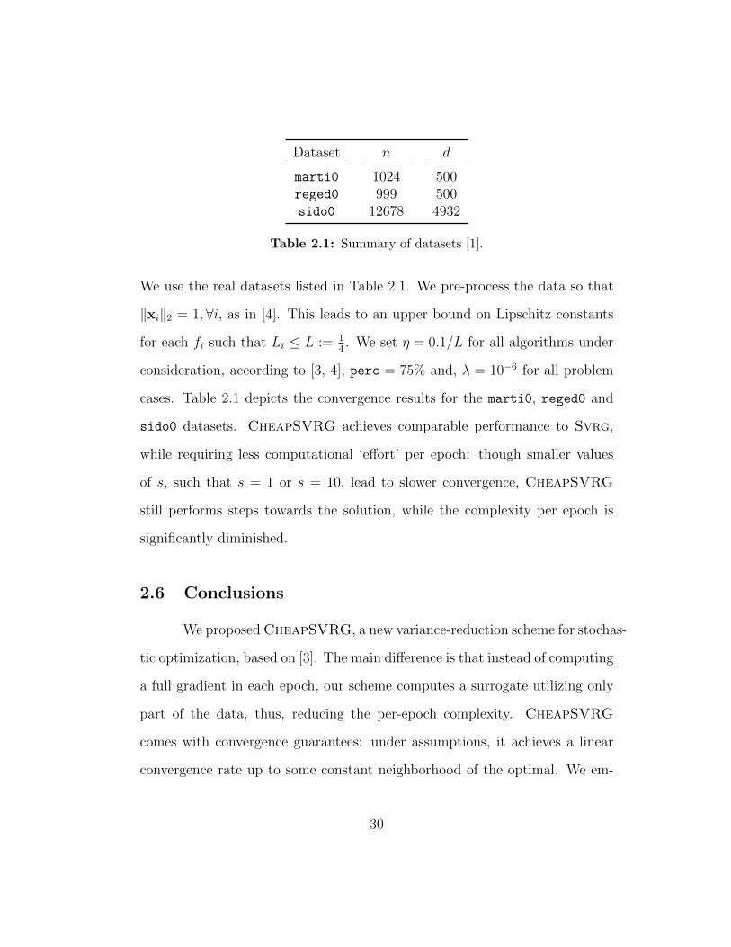
Dataset n d
marti0 1024 500reged0 999 500sido0 12678 4932
Table 2.1: Summary of datasets [1].
We use the real datasets listed in Table 2.1. We pre-process the data so that
‖xi‖2 = 1,∀i, as in [4]. This leads to an upper bound on Lipschitz constants
for each fi such that Li ≤ L := 14. We set η = 0.1/L for all algorithms under
consideration, according to [3, 4], perc = 75% and, λ = 10−6 for all problem
cases. Table 2.1 depicts the convergence results for the marti0, reged0 and
sido0 datasets. CheapSVRG achieves comparable performance to Svrg,
while requiring less computational ‘effort’ per epoch: though smaller values
of s, such that s = 1 or s = 10, lead to slower convergence, CheapSVRG
still performs steps towards the solution, while the complexity per epoch is
significantly diminished.
2.6 Conclusions
We proposed CheapSVRG, a new variance-reduction scheme for stochas-
tic optimization, based on [3]. The main difference is that instead of computing
a full gradient in each epoch, our scheme computes a surrogate utilizing only
part of the data, thus, reducing the per-epoch complexity. CheapSVRG
comes with convergence guarantees: under assumptions, it achieves a linear
convergence rate up to some constant neighborhood of the optimal. We em-
30
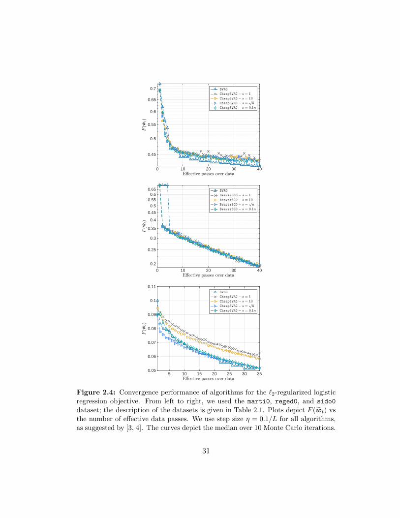
E,ective passes over data0 10 20 30 40
F(e w t)
0.45
0.5
0.55
0.6
0.65
0.7 SVRG
CheapSVRG ! s = 1
CheapSVRG ! s = 10
CheapSVRG ! s =p
n
CheapSVRG ! s = 0:1n
E,ective passes over data0 10 20 30 40
F(e w t)
0.2
0.25
0.3
0.35
0.4
0.45
0.50.55
0.60.65 SVRG
BeaverSGD ! s = 1
BeaverSGD ! s = 10
BeaverSGD ! s =p
n
BeaverSGD ! s = 0:1n
E,ective passes over data5 10 15 20 25 30 35
F(e w t)
0.05
0.06
0.07
0.08
0.09
0.1
0.11SVRG
CheapSVRG ! s = 1
CheapSVRG ! s = 10
CheapSVRG ! s =p
n
CheapSVRG ! s = 0:1n
Figure 2.4: Convergence performance of algorithms for the `2-regularized logisticregression objective. From left to right, we used the marti0, reged0, and sido0
dataset; the description of the datasets is given in Table 2.1. Plots depict F (wt) vsthe number of effective data passes. We use step size η = 0.1/L for all algorithms,as suggested by [3, 4]. The curves depict the median over 10 Monte Carlo iterations.
31

pirically evaluated our method and discussed its strengths and weaknesses.
There are several future directions. In the theory front, it would be
interesting to maintain similar convergence guarantees under fewer assump-
tions, extend our results beyond the smooth convex optimization, e.g., to the
proximal setting, or develop distributed variants. Finally, we seek to apply
our CheapSVRG to large-scale problems, e.g., for training large neural net-
works. We hope that this will help us better understand the properties of
CheapSVRG and the trade-offs associated with its various configuration pa-
rameters.
32

Chapter 3
On the Generalization of Adaptive Methods
Over-parameterization and adaptive methods have played a crucial role
in the success of deep learning in the last decade. The widespread use of
over-parameterization has forced us to rethink generalization by bringing forth
new phenomena, such as implicit regularization of optimization algorithms
and double descent with training progression. A series of recent works have
started to shed light on these areas in the quest to understand – why do neural
networks generalize well? The setting of over-parameterized linear regression
has provided key insights into understanding this mysterious behavior of neural
networks.
In this paper, we aim to characterize the performance of adaptive meth-
ods in the over-parameterized linear regression setting. First, we focus on
two sub-classes of adaptive methods depending on their generalization perfor-
mance. For the first class of adaptive methods, the parameter vector remains
in the span of the data and converges to the minimum norm solution like
Parts of this chapter was published in the Integration of Deep Learning Theories Work-shop at Neurips, 2018 and is also available at [42]. The author was a part of formulatingthe problem, analyzing the theory, designing the experiments, writing up the results, andperforming the simulations presented in the paper.
33
gradient descent (GD). On the other hand, for the second class of adaptive
methods, the gradient rotation caused by the pre-conditioner matrix results in
an in-span component of the parameter vector that converges to the minimum
norm solution and the out-of-span component that saturates. Our experiments
on over-parameterized linear regression and deep neural networks support this
theory.
3.1 Introduction
The success of deep learning has uncovered a new mystery of benign
overfitting [43, 44], i.e., systems with a large number of parameters can not
only achieve zero training error but are also able to generalize well. Also,
over-parameterized systems exhibit a double descent-behavior [43, 45]; as the
number of parameters/epochs increases, the test error first decreases, then in-
creases before falling again. This goes against the conventional wisdom of
overfitting in machine learning, which stems from the classical bias-variance
tradeoff [46, 47, 48].
In the absence of explicit regularization, a typical over-parameterized
setting possesses multiple global minima. Classical gradient descent based
methods can achieve one of these many global minima [49, 50, 51], however not
all optima generalize equally. [52, 53, 54] suggest many practical approaches
to improve generalization; however, there remains a considerable gap between
theory and practice [55, 49].
In this paper, we will focus on two categories of optimization algo-
34

rithms: pure gradient descent based (non-adaptive1) methods and adaptive
methods. The primary distinguishing factor between these two methods is
determined by the update step. For the class of non-adaptive methods, the
expected gradient update step is given as follows:
E [w(t+ 1)|w(t)] = w(t)− η∇f(w(t)), (3.1)
where w(t) indicates the estimate of the underlying parameter vector, η repre-
sents the learning rate and f(w(t)),∇f(w(t)) represent the loss function and
its gradient, respectively. Popular methods like gradient descent, stochastic
gradient descent (SGD), batch gradient descent fall under this class. Training
any model using non-adaptive methods involves tuning over many hyperpa-
rameters, of which step size is the most essential one [29, 56]. The step size
could be set as constant, or could be changing per iteration η(t) [53], usually
based on a predefined learning rate schedule [25, 57, 58].
During the past decade, we have also witnessed the rise of a family of
algorithms called adaptive methods that argue for automatic hyper-parameter
adaptation [59] during training (including step size). The list includes Ada-
Grad [60], Adam [61], AdaDelta [62], RMSProp [63], AdaMax [61], Nadam
[64], just to name a few. These algorithms utilize current and past gradi-
ent information ∇f(w(i))ki=t, for t < k, to design preconditioning matrices
D(t) 0 that better pinpoint the local curvature of the objective function as
1Now onwards, optimization methods that satisfy equation (3.1) will be referred to asnon-adaptive purposes.
35

follows:
E [w(t+ 1)|w(t)] = w(t)− ηD(t)∇f(w(t)) (3.2)
Usually, the main argument for using adaptive methods is that D(t) elimi-
nates pre-setting a learning rate schedule, or diminishes initial bad step size
choices, thus, detaching the time-consuming part of step size tuning from the
practitioner [65].
[66] was one of the first papers to discuss the implicit bias introduced
by optimization methods for over-parameterized systems and how the choice
of optimization algorithm affects the global minima it attains. However, the
generalization behavior of these optimization methods remains a mystery. As a
result, researchers have re-focussed their attention on understanding the most
straightforward over-parameterized setting of linear regression [43, 67, 68, 44]
as a first step in unraveling the mysterious behavior of neural networks.
Gradient descent-based methods converge to the minimum norm inter-
polated solution [44] for over-parameterized linear regression. Under certain
assumptions on the data distribution, the minimum norm solution achieves
near-optimal accuracy for unseen data [43]. Unlike SGD, the presence of D(t)
in adaptive methods can alter the span of the final converged solution in the
presence of any non-trivial initialization, which makes the task of commenting
on adaptive methods challenging.
Despite being a key reason behind the success of deep learning, the
convergence behavior of adaptive methods is not well understood. The con-
36

d = 50 GD AM1 AM2 AM3
n = 10Training Error 1.27 · 10−28 1.42 · 10−29 8.64 · 10−4 8.64 · 10−29
Test Error 81.56 76.94 79.62 81.65‖w −w∗‖ 9.08 8.92 9.03 9.08
n = 40Training Error 4.77 · 10−5 6.07 · 10−7 3.31 · 10−3 8.64 · 10−4
Test Error 18.62 19.56 20.35 18.65‖w −w∗‖ 4.31 4.37 4.51 4.31
Table 3.1: Table illustrating differing generalization guarantees of three distinctAdaptive Methods (AM) with SGD in over-parameterized setting, i.e. d > n, wheren: number of examples, d: dimension,
vergence bounds for most adaptive methods hold for only a specific pre-
conditioner matrix [61, 69, 66]. Besides, theoretical guarantees for adaptive
methods often minimize regret [70, 60], which makes it further challenging to
comment on the generalization of adaptive methods. As a result, the gener-
alization of adaptive methods for a general D(t) remains an open problem
even for an over-parameterized linear regression setting. In this paper, we
aim to explicitly characterize the sub-class of adaptive methods that mimic
the convergence, and generalization behaviors seen in SGD and the sub-class
that does not. In addition, we observe a double descent like phenomena for a
sub-class of adaptive methods as the number of training epochs increases.
In this paper, we would like to understand how adaptive methods af-
fect generalization guarantees of over-parameterized problems. To motivate
this, we consider a toy example for simple linear regression in the under-
determined/over-parameterized framework in Table 3.1. As is evident, some
adaptive methods have the same generalization as SGD, while others can yield
37
quite different generalization guarantees.
Key Contributions: For the theoretical contribution, we focus on over-
parameterized linear regression. Here, plain gradient descent methods con-
verge to the minimum Euclidean norm solution, while adaptive methods may
or may not. In this paper, we provide explicit conditions on the structure
of pre-conditioner matrices, D(t), which allow us to distinguish between two
classes of adaptive methods, the ones which behave similarly to SGD and the
ones that do not. Based on these conditions, we compare the generalization
performance between adaptive and non-adaptive methods.
For the experimental component, we begin by revisiting the mystery
posed by Table 3.1, and demonstrate that the experimental results are in line
with our theoretical guarantees. Further, we show using a toy example that the
adaptive methods can have a superior generalization performance than SGD.
The discussion “which method is provably better”, however, is inconclusive and
ultimately depends on the problem/application at hand. Lastly, we empirically
demonstrate the validity of our claims for over-parameterized neural networks
as well and recommend exercising caution when proposing or choosing adaptive
methods for training, depending on the goal in hand.
3.2 Problem Setup
Notation: For any matrixA ∈ Rm×n, Apq indicates the element correspond-
ing to the p-th row and q-th column. The rank(A) denotes the rank of A.
38

For a sequence of matrices A0 to An, we have the definition∏i
k=i+mAk =
A(i+m)A(i+m−1) . . .Ai. Note that, a(t) indicates the value of the the function
a(·) after the t-th update. Note that λ without any subscript indicates the
regularizer, and λi with a subscript denotes the ith eigenvalue. We consider
an over-parameterized noisy linear regression (possibly with regularization),
where the relationship between the data matrix X ∈ Rn×d, the noise vector
ζ ∈ Rn, and the labels y ∈ Rn is as follows:
y = Xw? + ζ. (3.3)
We are concerned with the following optimization problem:
f(w) = arg minw
E[‖y −Xw‖2
]+ λ
2‖w‖2
2
. (3.4)
In particular, we study the convergence of the following iterative updates
w(t+ 1) = w(t)− ηD(t)∇f(w(t)), (3.5)
where the pre-conditioner matrices are bounded, positive definite and hence
full rank; i.e., inft rank(D(t)) = d.
There are two different settings, depending on the number of samples
and dimension:
• Over-parameterized case: The system is assumed over-parameterized;
if R = rank(X) < d or there are more parameters than the number of
effective samples: d ≥ n. In this case, assuming that X is in general
position, XX> is full rank.
39
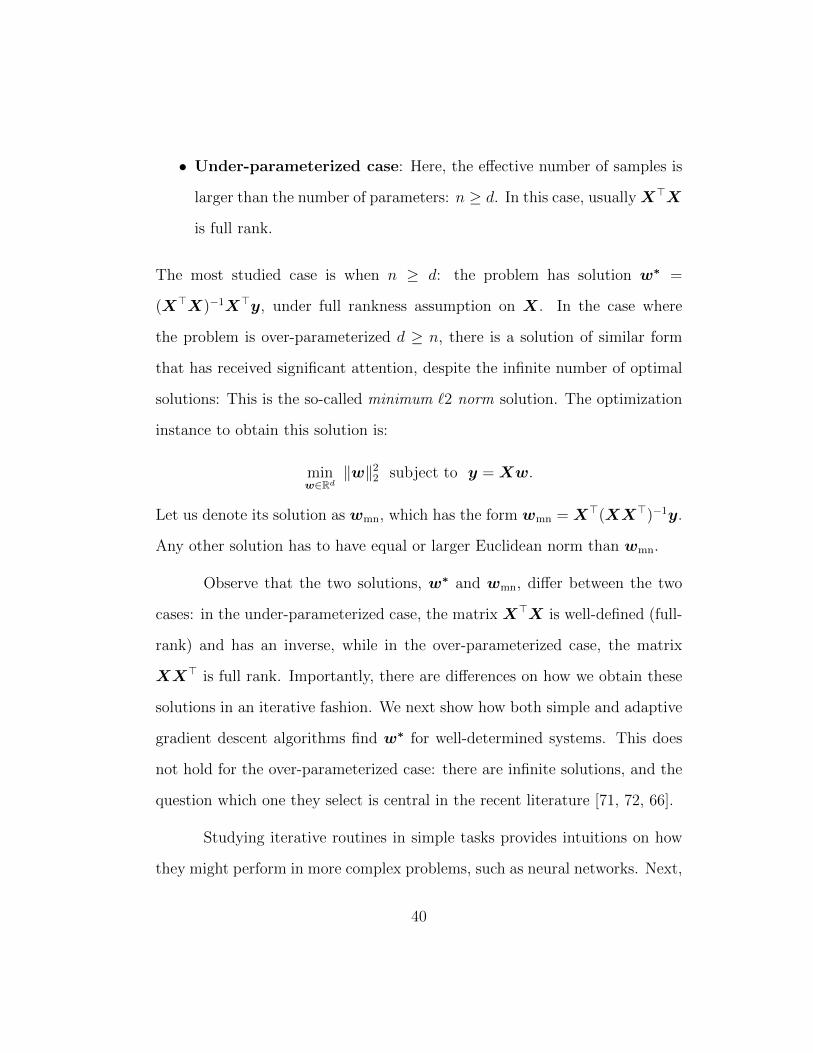
• Under-parameterized case: Here, the effective number of samples is
larger than the number of parameters: n ≥ d. In this case, usuallyX>X
is full rank.
The most studied case is when n ≥ d: the problem has solution w∗ =
(X>X)−1X>y, under full rankness assumption on X. In the case where
the problem is over-parameterized d ≥ n, there is a solution of similar form
that has received significant attention, despite the infinite number of optimal
solutions: This is the so-called minimum `2 norm solution. The optimization
instance to obtain this solution is:
minw∈Rd
‖w‖22 subject to y = Xw.
Let us denote its solution as wmn, which has the form wmn = X>(XX>)−1y.
Any other solution has to have equal or larger Euclidean norm than wmn.
Observe that the two solutions, w∗ and wmn, differ between the two
cases: in the under-parameterized case, the matrix X>X is well-defined (full-
rank) and has an inverse, while in the over-parameterized case, the matrix
XX> is full rank. Importantly, there are differences on how we obtain these
solutions in an iterative fashion. We next show how both simple and adaptive
gradient descent algorithms find w∗ for well-determined systems. This does
not hold for the over-parameterized case: there are infinite solutions, and the
question which one they select is central in the recent literature [71, 72, 66].
Studying iterative routines in simple tasks provides intuitions on how
they might perform in more complex problems, such as neural networks. Next,
40

we set the background with the well-known under-parameterized linear regres-
sion, before we move onto the over-parameterized case.
3.2.1 Non-adaptive Methods in Under-parameterized Linear Re-gression
Here, n ≥ d and X>X is assumed to be full rank. Simple gradient
descent with step size η > 0 satisfies: w(t + 1) = w(t) − η · ∇f(w(t)) =
w(t)− ηX>(Xw(t)− y). Unfolding for T iterations, we get:
w(T ) =
(t∑i=1
(−1)i−1 ·(t
i
)· ηi · (X>X)i−1
)X>y.
The expression in the parentheses satisfies:
T∑i=1
(−1)i−1 ·(T
i
)· ηi · (X>X)i−1 = (−X>X)−1 ·
((I − ηX>X)T − I
)Therefore, we get the closed form solution:
w(T ) = (−X>X)−1 ·((I − ηX>X)T − I
)X>y
. In order to prove that gradient descent converges to the minimum norm
solution, we need to prove that:
(I − ηX>X)T − I = −I ⇒ (I − ηX>X)Tn,T large−→ 0.
This is equivalent to showing that ‖(I − ηX>X)T‖2 → 0. From optimization
theory [73], we need η < 1λ1(X>X)
for convergence, where λi(·) denotes the
eigenvalues of the argument. Then, H := I − ηX>X ∈ Rd×d has spectral
norm that is smaller than 1, i.e., ‖H‖ ≤ 1. Combining the above, we use the
following theorem.
41
Theorem 3.2.1 (Behavior of square matrix ‖MT‖2 ). [74, 75] Let M
is a d × d matrix. Let τ(M ) = maxi |λi(M)| denote the spectral radius of
the matrix M . Then, there exists a sequence ε(t) ≥ 0 such that: ‖MT‖2 ≤
(τ(M) + ε(t))T , and limT→∞ ε(t) = 0.
Using the above theorem, H has τ(H) < 1. Further, for sufficiently
large t < T , ε(t) has a small value such that τ(H) + ε(t) < 1; i.e., after some
t1 < T , (τ(H) + εt1)t1 , will be less than zero, converging to zero for increasing
t1. As T is going towards infinity, this concludes the proof, and leads to the
left inverse solution: w∞ = (−X>X)−1 · (−I)X>y = (X>X)−1X>y ≡ w∗,
as T →∞. This is identical to the closed for solution of linear regression.
3.2.2 Adaptive Methods in Under-parameterized Linear Regres-sion
When D(t) is varying, we end up with the following proposition (folk-
lore); the proof is in Section B.3.:
Proposition 3.2.2. Consider the under-parameterized linear regression set-
ting with data matrix X, noise ζ, and regularizer λ > 0. Suppose for all t ≥ 0,
the pre-conditioner matrix D(t) is positive definite, i.e. D(t) 0. Assume
the recursion w(t + 1) = w(t) − ηD(t)∇f(w(t)). Then, after T iterations,
w(t) satisfies:
w(t) =(−X>X
)−1 ·(
0∏i=T−1
(I − ηX>XD(i)
)− I
)X>y.
42

Using Theorem 3.2.1, we can again infer that, for sufficiently large T
and for sufficiently small η < maxi1
λ1(X>XDi), such that ‖I − ηX>XDi‖ <
1 ∀ i, we have:∏0
i=T−1
(I − ηX>XDi
)→ 0. Thus, for sufficiently large T
and assuming η < maxi1
λ1(X>XDi), ∀i: w∞ = (X>X)−1 ·X>y ≡ w∗, which
is the same as the plain gradient descent approach. Thus, in this case, under
proper η assumptions (which might seem stricter than plain gradient descent),
adaptive methods have the same generalization capabilities as gradient descent.
3.3 Over-parameterized linear regression
Over-parameterized systems possess more degrees of freedom than the
number of training samples. As a result, we know that standard gradient
descent based methods fit perfectly to the training set.
3.3.1 Performance on Training Set for Non-Adaptive Methods
For completeness, we briefly provide the analysis for the over-parameterized
setting, where d ≥ n and XX> is assumed to be full rank. By inspection,
unfolding gradient descent recursion gives after T iterations:
w(T ) = X>
(T∑i=1
(−1)i−1 ·(T
i
)· ηi · (XX>)i−1
)y.
Similarly, the summation can be simplified to:
T∑i=1
(−1)i−1 ·(T
i
)· ηi · (XX>)i−1 = (−XX>)−1 ·
((I − ηXX>)K − I
),
and, therefore:
w(T ) = X>(−XX>)−1 ·((I − ηXX>)K − I
)y.
43

Under similar assumption on the spectral norm of (I − ηXX>)K and using
Theorem 3.2.1, we obtain the right inverse solution: w∞ = X>(−XX>)−1 ·
(−I)y = X>(XX>)−1y ≡ wmn, as K → ∞. Bottomline, in both cases,
gradient descent converges to left and right inverse solutions, related to the
Moore-Penrose inverse.
Before we discuss the generalization of adaptive methods in over pa-
rameterized settings, let us first answer the following question: what is the
predictive power of adaptive methods within the training set?
3.3.2 Performance on Training Set for Adaptive Methods
For linear regression with `2 norm regularization, we observe that adap-
tive methods with any full rank pre-conditioner matrix D(t) will converge to
the same solution as its non-adaptive counterpart and thus mimic their per-
formance. However, for unregularized linear regression, adaptive methods can
converge to entirely different solutions than SGD. Before we discuss general-
ization, we will first show that both SGD and adaptive methods can achieve
zero training error despite attaining different stationary points.
Proposition 3.3.1. Consider the over-parameterized linear regression setting
with data matrix X, noise ζ, and regularizer λ > 0. Suppose for all t ≥ 0, the
pre-conditioner matrix D(t) is positive definite, i.e. D(t) 0. Assume the
recursion w(t + 1) = w(t) − ηD(t)∇f(w(t)). If D(t) is positive definite for
44

all t and the regularizer λ = 0, then,
limt→∞
y(t) = y.
where y(t) = Xw and w = limT→∞wt.
Proposition 3.3.1 implies that adaptive methods with full-rank positive
definite preconditioners perform as well as their pure gradient based counter
parts when it comes to fitting their training data. However, this proposition
gives no information regarding the distance between the converged w(t) and
w?.
Proposition 3.3.2. Consider the over-parameterized linear regression setting
with data matrix X, noise ζ, and regularizer λ > 0. Suppose for all t ≥ 0, the
pre-conditioner matrix D(t) is positive definite, i.e. D(t) 0. Assume the
recursion w(t+ 1) = w(t)− ηDt∇f(w(t)). If D(t) is positive definite for all
t and the regularizer satisfies λ > 0, then,
limt→∞
w(t) =(X>X + λI
)−1X>y.
Proposition 3.3.2 implies that for the regularized case, the problem be-
comes strongly convex and the adaptive methods converge to the same solution
as their SGD counterparts under certain conditions.
To summarize, for linear regression with `2-norm regularization, we ob-
serve that adaptive methods with any full rank pre-conditioner matrix D(t)
will converge to the same solution as its non-adaptive counterpart and thus
45

mimic their performance. However, for unregularized linear regression, adap-
tive methods can converge to entirely different solutions than SGD. Both SGD
and adaptive methods can achieve zero training error despite attaining differ-
ent stationary points. This leads us to the following question: What is the
predictive power of adaptive methods on unseen data for over-parameterized
linear regression?
3.4 Performance on Unseen Data
Our primary focus in this chapter is to understand the generalization
capabilities of adaptive methods. We observe that the generalization depends
on two key factors: i) Does w? lie in the span of the data matrix, X? ii)
How does pre-multiplying with the pre-conditioner matrix alter the span of final
converged w?
3.4.1 Spectral Representation
The switch to the spectral domain allows us to simplify and under-
stand the relationship between the final converged solution with the span
of data matrix X, pre-conditioner matrix D(t) and the initialization w(0).
We express the data matrix using its singular value decomposition (SVD):
X =∑R
r=1 λrurvTr , λr 6= 0 for all r where λr,ur,vr represent the rth largest
eigenvalue and the corresponding right and left eigenvectors respectively. We
complete the basis using the left eigenvectors of the data matrix to form a com-
plete orthogonal spectral basis of Rd, vr : r = 1 . . . , d form the basis vectors
46

and denote it by V . Similarly, U forms the complete orthogonal spectral basis
of Rn using the right eigenvectors of the data matrix as ur : r = 1 . . . , n.
The eigenvalue matrix is Λ where Λrr = λr if 1 ≤ r ≤ R and 0 otherwise. We
next express useful quantities in the above bases in Table 3.2.
Data matrix X = UΛV T
True parameter w? = V w?
Noise vector ζ = Uζ
Adaptive pre-conditioner matricesD(t) =
∑dr=1
∑ds=1 Drs(t)vrv
Ts ,
D(t) = V TD(t)V , D(t) ∈ Rd×d
Weight vectors w(t) = V w(t)
Table 3.2: Notation in spectral domain
The definition of adaptive pre-conditioner matrices in the above table
holds since V represents a complete orthogonal spectral basis of Rd. Addi-
tionally, we also have the following property, where we show that pre- and
post-multiplication by an orthogonal matrix V does not alter the eigenvalues
of the original matrix. In other words, we have the following proposition:
Proposition 3.4.1. The set of eigenvalues for D(t) is identical to the set of
eigenvalues of D(t).
The proof of Proposition 3.4.1 is available in Appendix.
3.4.2 Closed Form Expression for the Iterates
Our objective is to understand how the iterates evolve depending on the
space spanned by the data matrix. First, we establish a closed-form expression
47

for the updates of the vector w(t).
Proposition 3.4.2. Consider the over-parameterized linear regression setting
with data matrix X, noise ζ, and regularizer λ > 0. If the pre-conditioner
matrix D(t) 0 for all t ≥ 0, then, for any T ≥ 0, the iterate w(T ) admits
the following closed form expression:
w(T ) =T−1∏i=0
(I − ηD(i)(Λ2 + λI)
)w(0)
+T−1∑i=0
T−1∏j=(i+1)
(I − ηD(j)(Λ2 + λI)
)ηD(i)(Λ2w? + Λζ) (3.6)
The final expression of w(T ) implies that the final solution depends on the
initialization point, the span of the data matrix in Rd space, and the pre-
conditioner matrix. Further, the closed-form indicates that the presence of
pre-conditioning matrices D(j) may cause w(t) to lie outside of the span of
the data in the complete Rd space.
We observe that the presence or absence of regularizer can significantly
alter the stationary points to which adaptive methods converge. In the pres-
ence of `2-norm regularization, we observe that the adaptive methods converge
to the same solution independent of the initialization or the step-size. How-
ever, in the absence of regularization, things are not as straight-forward. Here,
we will try to capture the convergence of over parameterized linear regression
using dynamics described by equation (3.5).
48

3.4.3 `2-norm Regularized Linear Regression.
In presence of `2-norm regularization, the over-parameterized linear
regression problem becomes strongly convex and possesses a unique global
optima. Proposition 2 serves a sanity check; where we show the convergence
to this unique optima for any positive definite pre-conditioner matrix D(t) in
the spectral domain.
Proposition 3.4.3. Consider the over-parameterized linear regression setting
with data matrix X, noise ζ, and regularizer λ > 0. Assume the recursion
w(t + 1) = w(t) − ηDt∇f(w(t)). Suppose for all t ≥ 0, the pre-conditioner
matrix D(t) 0, and the learning rate satisfies
η ∈(
0, 2(λmax(D(t))(λ2
max(X) + λ))−1)
where λmax(·) indicates the maximum eigenvalue. Then, w(t) converges to the
following fixed point
limt→∞
w(t) = (Λ2 + λI)−1(Λ2w? + Λζ). (3.7)
Proposition 3.4.3 states that like the gradient descent based methods,
the adaptive methods will perfectly capture the component of the generative
w∗ that lies in the subspace formed by the data matrix. In other words, with
regularization the parameter vector converges in the span of X.
In the proof of the proposition presented in the Appendix, we use con-
traction properties to show convergence where λ > 0 plays a significant role.
49
Further, as inft rank(D(t)), a simple fixed-point analysis provides us with the
in-span component and shows that for λ > 0 there is no out-of-span compo-
nent of the solution. Note that this proposition acts as a proof of concept
for the well-known result that adaptive methods and non-adaptive methods
converge to the same solution in the presence of `2-norm regularization.
Lastly, different regularization techniques alter the implicit bias of the
final converged solution differently. The claims made in this sub-section are
only valid for `2-norm regularization.
3.4.4 Unregularized Linear Regression.
Next, we focus on the problem of unregularized linear regression in the
over-parameterized regime. The optimization problem with squared loss is no
longer strongly convex, and there are infinite solutions that can achieve zero
training error. In this case, the convergence of unregularized linear regression
depends on the initialization w(0). Further, as λmin(D(t)Λ2) = 0 we cannot
directly prove (using contraction mapping) convergence for general unregular-
ized over-parameterized linear regression. However, when the pre-conditioner
matrices satisfy a block matrix structure, then we can say something about
the converged solution. Note that most of the popular adaptive algorithms
[60, 61, 70, 76] satisfy the block matrix structure.
The out-of-span component behavior depends subtly on the interplay of
the pre-conditioner matrices and the span of data. Now, we establish sufficient
conditions on the class of pre-conditioner matrices for which the convergence
50
is guaranteed (for more details refer Appendix).
We define some notations useful to state our main theorems. We use
w(1)(∞) = limt→∞
w(1)(t) to denote the in-span component, and w(2)(∞) =
limt→∞
w(2)(t) to denote the in-span component of the stationary point.2 Let,
e(1)(t) = ‖w(1)(∞) − w(1)(i)‖2 = O(
1
tβ
)be the `2-norm distance of in-span
component of the iterate from the in-span stationary point at time t ≥ 1. We
further define:
Definition 3.4.4. For a data matrix X and an adaptive method, with pre-
conditioning matrices D(t) : t ≥ 1, we call the adaptive method (α, β)-
converging on data, for any α, β ≥ 0, if and only if: i) the out-of-span com-
ponent of the pre-condition matrices decays as |λmax(D2(t))| = O(
1
tα
); ii)
the in in-span component of the iterates converges as, e(1)(t) = O(
1tβ
)(under
Eq. (3.5)).
Any adaptive method with a pre-conditioner matrix that lies entirely
in the span of the matrix will have α set to∞. Full-matrix Adagrad, GD, and
Newton all fall under this class of adaptive methods. Popular adaptive meth-
ods, such as diagonalized Adagrad, RMSProp, and methods with a diagonal
pre-conditioner matrix with non-zero entries, the convergence depends on the
rate of decay of both the D2(t) as well as the rate of decay of the error of the
in-span component.
2Note that w(2)(∞) ∈ (R ∪ ∞)d for i = 1, 2, as we can not assume convergence of theiterates a pirori.
51
Theorem 3.4.5. Consider the problem of over-parameterized linear regression
with data matrix X and noise ζ in the absence of regularization λ = 0. Assume
the recursion w(t + 1) = w(t) − ηDt∇f(w(t)). If the preconditioner matrix
D(t) 0 ∀t ≥ 0, and η ∈(
0,2
λmax(D(t))λ2max(X)
), then in-span component
of w(t) converges as follows
w(1)(∞) = (w∗(1) + Λ−1(1)ζ(1)).
Furthermore, for an adaptive method (in Eq. (3.5)) which is (α, β)-converging
on data, if α + β > 1 the out-of-span component converges to a stationary
point that satisfies
‖w(2)(∞)− w(2)(0)‖2 ≤ O(‖w(1)(0)‖2 +
1
α + β − 1
).
Remark on Theorem 3.4.5: Let us deconstruct the claims made in
Theorem 3.4.5. Theorem 1 says that if η is set appropriately, then adaptive
methods will perfectly fit the noisy training data. This is consistent with the
claims in [44]. The convergence of out-of-span component depends on the de-
cay rate of the pre-conditioner matrix D2(t) as well as the decay rate of the
error term in the in-span component e(1)(t) = ‖(w∗(1)+Λ−1(1)ζ(1))−w(1)(i)‖2. For
the simple case, when β ≥ 1 and D(2)(t) = 0 for all t, we have that the out-of-
span component converges to w(2)(0). Next, if limT→∞∑T
t=0 max |λ(D(2)(t))| <
∞ and α + β ≥ 1, then the out-of-span component converge. For all other
cases, it is difficult to comment whether the out-of-span component will con-
verge or diverge. Specifically, for α + β < 1, we may not have divergence as
the pre-conditioner matrices may align cancel the cumulative errors.
52
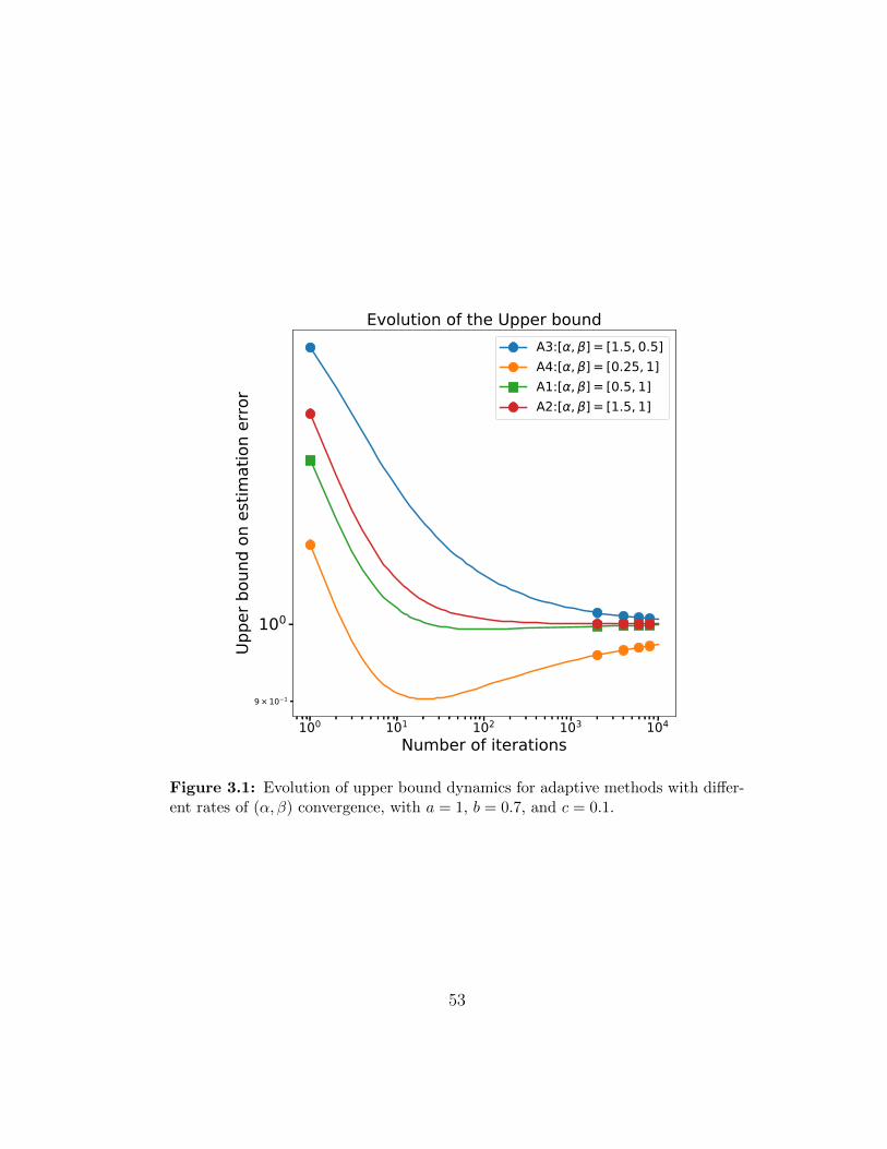
100 101 102 103 104
Number of iterations
100
9 × 10 1
Uppe
r bou
nd o
n es
timat
ion
erro
r
Evolution of the Upper boundA3:[ , ] = [1.5, 0.5]A4:[ , ] = [0.25, 1]A1:[ , ] = [0.5, 1]A2:[ , ] = [1.5, 1]
Figure 3.1: Evolution of upper bound dynamics for adaptive methods with differ-ent rates of (α, β) convergence, with a = 1, b = 0.7, and c = 0.1.
53

Remark on Dynamics: It is also interesting to note that the error in the
in-span component converges to 0 and the error in the out-of-span component
increases and saturates to a particular value. Our derived upper bound on the
training error at time T for an adaptive method that is (α, β) converging on
data is given as :
a+b
(T + 1)β
(1− c
α + β − 1
1
(T + 1)α−1
)for appropriate constants a, b, c > 0. The dynamics is shown in the Figure 5.6.
Depending on the values of the constants, α, and β, adaptive methods demon-
strate variable convergence dynamics.
3.5 Experiments
In this section, we focus on replicating the theoretical claims made in
the previous parts using synthetic experiments for over-parameterized linear
regression. Next, we show that these observations can be extended to the deep
learning setup as well. We empirically compare two classes of algorithms:
• Plain gradient descent algorithms, including the mini-batch stochastic gra-
dient descent and the accelerated stochastic gradient descent, with constant
momentum.
• Adaptive methods like AdaGrad [60], RMSProp [63], and Adam [61], and
the AdaGrad variant. Adaptive methods can include anything with a time-
varying pre-conditioner matrix.
54

d = 50 GD AM1 AM2 AM3
D(t) I D1(t) D2(t) PX(D1(t))
n = 10Training Error 1.27 · 10−28 1.42 · 10−29 8.64 · 10−4 8.64 · 10−29
Test Error 81.56 76.94 79.62 81.65‖w −w∗‖ 9.08 8.92 9.03 9.08
n = 40Training Error 4.77 · 10−5 6.07 · 10−7 3.31 · 10−3 8.64 · 10−4
Test Error 18.62 19.56 20.35 18.65‖w −w∗‖ 4.31 4.37 4.51 4.31
Table 3.3: Illustrating the varying performances of adaptive methods for over-parameterized linear regression. The final values are the average of 5 runs. AM1:Diagonalized Adagrad, AM2: Adagrad (AM1) Variant (where we square the di-agonal terms instead of taking the square root), AM3: Projected version of AM1onto the span of X. For AM3, D2(t) = 0, ∀ t and consistent with Theorem 3.4.5 itconverges to the same point as SGD. AM1 and AM2 satisfy the (α, β) convergencecriterion leading to convergence to a different point and different generalization thanSGD.
3.5.1 Linear Regression
In the first part, we consider a simple linear regression example gener-
ated where the elements of both X and ζ are generated from N (0, 1) distri-
bution in an i.i.d. manner. First, we revisit Table 3.1 and demonstrate the
varying performances of different adaptive methods.
In the first set of experiments, we showed how adaptive methods con-
verging to a different solution might lead to solutions farther from w∗b , i.e.
with higher L2-norm . Thus, the pre-conditioner matrices satisfying Dij(t) =
0,D(t) 0 have different generalization than their gradient based counter-
parts. In this section, we empirically demonstrate that pre-conditioner ma-
trices of the form: Dij(t) = 0,D(t) 0 can guarantee better generalization
than gradient based methods depending on the problem in hand. As a direct
55

consequence of this, we show that solutions with a minimum norm should not
be used as a yardstick to guarantee good generalization.
Here, we show in Table 3.3 and Figure 3.2 that different adaptive meth-
ods can yield better performance in terms of test error.
3.5.1.1 Counter Example
Next, we consider a linear regression problem with binary outputs,
which is a variant of the example proposed in [71]. In this section, we show
that even in terms of test accuracy, adaptive algorithms can yield better gen-
eralization performance than SGD. This supports the claim made recently in
[77] for non-adaptive methods; the testing criterion can play a crucial role in
determining the generalization performance. We observe that this claim holds
for adaptive methods as well.
Toy example illustrating how to achieve different generalization from
gradient descent based methods: To prove otherwise, we could either
find a completely different counterexample (since adaptive methods do not
perform well in the one in [71]), or we find an alternative adaptive method
that performs well in that counter-example.
Here, we follow the second path and alter the previous counterexample
in [71] by slightly changing the problem setting: at first, we reduce the margin
between the two classes; the case where we increase the margin is provided
in the Appendix. We empirically show that gradient-descent methods fail
56
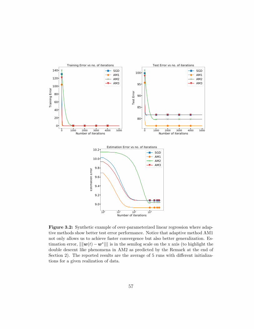
0 1000 2000 3000 4000 5000Number of iterations
0
20
40
60
80
100
120
140
Trai
ning
Erro
r
Training Error vs no. of iterationsSGDAM1AM2AM3
0 1000 2000 3000 4000 5000Number of iterations
80
85
90
95
100
Test
Erro
r
Test Error vs no. of iterationsSGDAM1AM2AM3
100 101 102 103
Number of iterations
9.0
9.2
9.4
9.6
9.8
10.0
10.2
Estim
atio
n Er
ror
Estimation Error vs no. of iterationsSGDAM1AM2AM3
Figure 3.2: Synthetic example of over-parameterized linear regression where adap-tive methods show better test error performance. Notice that adaptive method AM1not only allows us to achieve faster convergence but also better generalization. Es-timation error, ‖‖w(t)−w∗‖‖ is in the semilog scale on the x axis (to highlight thedouble descent like phenomena in AM2 as predicted by the Remark at the end ofSection 2). The reported results are the average of 5 runs with different initializa-tions for a given realization of data.
57

to generalize as well as adaptive methods –with a slightly different Dk than
AdaGrad. In particular, for the responses, we consider two classes yi ∈ ±`
for some ` ∈ (0, 1); i.e., we consider a smaller margin between the two classes.
One can consider classes in ±1, but the rest of the problem settings need
to be weighted accordingly. We selected to weight the classes differently in
order not to drift much from the couterexample from [71]. ` can take different
values, and still we get the same performance, as we show in the experiments
below.
(xi)j =
yi`, j = 1,
1, j = 2, 3,
1, j = 4 + 5(i− 1),
0, otherwise.
if yi = 1,
(xi)j =
yi`, j = 1,
1, j = 2, 3,
1, j = 4 + 5(i− 1),
· · · , 8 + 5(i− 1),
0, otherwise.
if yi = −1. (3.8)
Given this generative model, we construct n samples yi, xini=1, and
set d = 6n, for different n values. We compare two simple algorithms: i)i)i)
the plain gradient descent, for η =1
λ1(X>X); ii)ii)ii) the recursion w(t + 1) =
w(t)− ηD(t)X> (Xw(t)− y), where η is set as above, and D(t) follows the
rule:
D(t) = diag
1/
(t∑
j=t−J
∇f(w(j))∇f(w(j)) + ε
)2
0, for some ε > 0, and J < t ∈ N+ (3.9)
58

Observe that D(t) uses the dot product of gradients, squared. A variant of
this preconditioner is found in [78]; however our purpose is not to recommend
a particular preconditioner but to show that there are Dk that lead to better
performance than the minimum norm solution. We denote as wada, wadam and
wGD the estimates of the ADAM, Adagrad Variant (ADAVAR) and simple
gradient descent (GD), respectively.
The experiment obeys the following steps: i)i)i) we train both gradient
and adaptive gradient methods on the same training set, ii)ii)ii) we test models on
new data ytesti , xtest
i Qi=1. We define performance in terms of the classification
error: for a new sample ytesti , xtest
i and given wada, wadam and wGD, the only
features that are non-zeros in both xtesti and w’s are the first 3 entries [71, pp.
5]. This is due to the fact that, for gradient descent and given the structure
in X, only these 3 features affects the performance of gradient descent. Thus,
the decision rules for both algorithms are:
y adai = quant`
(wada
1 · ytesti + wada
2 + wada3
),
y GDi = quant`
(wGD
1 · ytesti + wGD
2 + wGD3
),
y adami = quant`
(wadam
1 · ytesti + wadam
2 + wadam3
),
where quant`(α) finds the nearest point w.r.t. ±`. With this example,
our aim is to show that adaptive methods lead to models that have better
generalization than gradient descent.
Table 3.4 summarizes the empirical findings. In order to cover a wider
range of settings, we consider n = [10, 50, 100] and set d = 6n, as dictated by
59

[71]. We generate X as above, where instances in the positive class, yi ∈ +`,
are generated with probability p = 7/8; the cases where p = 5/8 and p = 3/8
are provided in the appendix, and also convey the same message as in Table
3.4. Further details on the experiments are provided in the Appendix.
Algorithm GD ADAVAR ADAM
n = 10
` = 1/32Acc. (%) 63 100 91‖w −wmn‖2 1.015 · 10−16 4.6924 · 104 0.1007
` = 1/16Acc. (%) 53 100 87‖w −wmn‖2 1.7401 · 10−16 1.1504 · 103 0.0864
` = 1/8Acc. (%) 58 99 84‖w −wmn‖2 4.08 · 10−16 112.03 0.0764
n = 50
` = 1/32Acc. (%) 77 100 88‖w −wmn‖2 4.729 · 10−15 3.574 · 103 0.0271
` = 1/16Acc. (%) 80 100 89‖w −wmn‖2 6.9197 · 10−15 4.44 · 102 0.06281
` = 1/8Acc. (%) 91 100 89‖w −wmn‖2 9.7170 · 10−15 54.93 0.1767
Table 3.4: Prediction accuracy and distances from the minimum norm solution forplain gradient descent and adaptive gradient descent methods. We set p = 7/8 andJ = 10, as in the main text. The adaptive method uses Dk according to (3.9). Thedistances shown are median values out of 100 different realizations for each setting;the accuracies are obtained by testing 104 predictions on unseen data.
The proposed AdaGrad variant described in equation (3.9) falls under
the broad class of adaptive algorithms with Dk. However, for the counter
example in the AdaGrad variant neither satisfies the convergence guarantees
of Lemma 3.1 in [71, pp. 5], nor does it converge to the minimum norm solution
evidenced by its norm in Table 3.4.
Proposition 3.5.1. Suppose X>y has no zero components. Define D =
diag(|X>y|3) and assume there exists a scalar c such thatXD−1sign(X>y) =
60
cy. Then, when initialized at 0, the AdaGrad variant in (3.9) converges to the
unique solution w ∝D−1sign(X>y).
To buttress our claim that the AdaGrad variant in (3.9) converges to
a solution different than that of minimum norm (which is the case for plain
gradient descent), we provide the following proposition for a specific class of
problems3; the proof is provided in Appendix Section B.10.
3.5.2 Deep Learning
Next, we observe that the theoretical claims made for the generaliza-
tion of adaptive methods for over-parameterized linear regression extend over
to over-parameterized neural networks. We perform extensive experiments
on CIFAR-100 for CIFAR-100 datasets we explore four different architectures;
PreActResNet18 [5], MobileNet [6], MobileNetV2 [7], GoogleNet [7]. Comput-
ing weight norms of all layers is memory intensive and computationally expen-
sive typically, we use the weight vector norms on the last layer. We observe
that, like linear regression, here also adaptive methods can be clubbed into
different categories based on the evolution of their pre-conditioner matrices,
D(t). For deep learning experiments, we do not have a generative parameter.
We used the norm of the weights of the last layer as a surrogate for estima-
tion error to comment on the convergence of optimization algorithms. It is
evident that algorithms that have similar weight norms have similar training
loss performance; however the other side of the claim need not be true.
3Not the problem proposed in the counter-example 1 on pg 5.
61

We empirically compare two classes of algorithms:
• Plain gradient descent algorithms, including the mini-batch stochastic gra-
dient descent and the accelerated stochastic gradient descent, with constant
momentum.
• Adaptive methods like AdaGrad [60], RMSProp [63], and Adam [61], and
the AdaGrad variant. Adaptive methods can include anything with a vary-
ing pre-conditioning matrix.
In this section, we will extend the experiments to over-parameterized
and under-parameterized neural networks without regularization. We begin
with a detailed description of the datasets and the architectures we use along
with comprehensive set of experiments with hyperparameter tuning.
Name Network type DatasetM1-UP Shallow CNN + FFN MNISTM1-OP Shallow CNN + FFN MNISTC1-UP Shallow CNN + FFN CIFAR-10C1-OP ResNet18 CIFAR-10C2-OP PreActResNet18 CIFAR-100C3-OP MobileNet CIFAR-100C4-OP MobileNetV2 CIFAR-100C5-OP GoogleNet CIFAR-100
Table 3.5: Summary of the datasets and the architectures used for experiments.CNN stands for convolutional neural network, FF stands for feed forward network.More details are given in the main text.
MNIST dataset and the M1 architecture. Each experiment for M1 is
simulated over 50 epochs and 10 runs for both under- and over-parameterized
62

settings. The MNIST architectures consisted of two convolutional layers (the
second one with dropouts [79]) followed by two fully connected layers. M1-OP
had ∼ 73K parameters. Top row corresponds row to the M1-OP case. We plot
training errors and the test accuracy results on unseen data. For the M1-OP
case, SGD momentum performs less favorably compared to plain SGD, and
we conjecture that this is due to non-optimal tuning. In this case, all adaptive
methods perform similarly to SGD.
0 10 20 30 40 50Epochs
0.0
0.1
0.2
0.3
0.4
0.5
0.6
Loss
Training lossSGDSGD momentumAdagradAdagrad var.AdamRMSProp
0 10 20 30 40 50Epochs
92
93
94
95
96
97
98
99
Accu
racy
Accuracy
SGDSGD momentumAdagradAdagrad var.AdamRMSProp
0 25 50 75 100 125 150 175 200Epochs
0.00
0.25
0.50
0.75
1.00
1.25
1.50
1.75
2.00
Loss
Training lossSGDSGD momentumAdagradAdagrad var.AdamRMSProp
0 25 50 75 100 125 150 175 200Epochs
40
50
60
70
80
90
Accu
racy
Accuracy
SGDSGD momentumAdagradAdagrad var.AdamRMSProp
Figure 3.3: Accuracy results on unseen data, for different NN architectures anddatasets for over-parameterized configurations. Left two panels: Accuracy and train-ing loss for MNIST; Right two panels: Accuracy and training loss for CIFAR10.
63

CIFAR10 dataset and the C1 architecture. The over-parameterized
CIFAR-10 setting, C1-OP was trained over 200 epochs. Here, we implement a
Resnet [80] + dropout architecture (∼ 0.25 million parameters) 4 and obtained
top-1 accuracy of ∼ 93%. Adam and RMSProp achieves the best performance
than their non-adaptive counterparts for both the under-parameterized and
over-parameterized settings.
Figure 3.3, right panel, follows the same pattern with the MNIST data;
it reports the results over 10 Monte-Carlo realizations. Again, we observe
that AdaGrad methods do not perform as well as the rest of the algorithms.
Nevertheless, adaptive methods (such as Adam and RMSProp) perform simi-
larly to simple SGD variants. Further experiments on CIFAR-100 for different
architecture are provided in the Appendix.
CIFAR100 and other deep architectures (C2-5-OP). In this ex-
periment, we focus only on the over-parameterized case: DNNs are usually
designed over-parameterized in practice, with ever growing number of layers,
and, eventually, a larger number of parameters [81]. We again completed
10 runs for each of the set up we considered. C2-OP corresponds to Pre-
ActResNet18 from [5], C3-OP corresponds to MobileNet from [6], C4-OP is
MobileNetV2 from [7], and C5-OP is GoogleNet from [82]. The results are
depicted in Figure 3.4. After a similar hyper-parameter tuning phase, we se-
4Some parts of the code are from the following github repository was used for experi-ments: https://github.com/kuangliu/pytorch-cifar
64

0 20 40 60 80 100 120 140Epochs
0
50
100
150
200
250
300
Wei
ghts
nor
m
Weights norm
SGDSGD momentumAdagradAdagrad var.AdamRMSProp
0 20 40 60 80 100 120 140Epochs
0
20
40
60
80
100
120
140
160
Wei
ght n
orm
Weight norm
SGDSGD momentumAdagradAdagrad var.AdamRMSProp
0 25 50 75 100 125 150 175Epochs
0
5
10
15
20
25
30
Loss
Training lossSGDSGD momentumAdagradAdagrad var.AdamRMSProp
0 25 50 75 100 125 150 175Epochs
0
1
2
3
4Lo
ss
Training lossSGDSGD momentumAdagradAdagrad var.AdamRMSProp
0 25 50 75 100 125 150 175Epochs
0
10
20
30
40
50
60
70
Accu
racy
Accuracy
SGDSGD momentumAdagradAdagrad var.AdamRMSProp
0 25 50 75 100 125 150 175Epochs
10
20
30
40
50
60
Accu
racy
Accuracy
SGDSGD momentumAdagradAdagrad var.AdamRMSProp
Figure 3.4: Accuracy results on unseen data, for different NN architectures onCIFAR100. Left panel: Accuracy and training loss for PreActResNet18 in [5]; Rightpanel: Accuracy and training loss for MobileNet in [6] Top row: Weight vectors ofthe last layer, Middle row: Training Loss, Last row: Test Accuracy.
65

0 20 40 60 80 100 120 140Epochs
0
25
50
75
100
125
150
175
Wei
ght n
orm
Weight norm
SGDSGD momentumAdagradAdagrad var.AdamRMSProp
0 20 40 60 80 100 120 140Epochs
0
50
100
150
200
250
300
Wei
ght n
orm
Weight normSGDSGD momentumAdagradAdagrad var.AdamRMSProp
0 25 50 75 100 125 150 175Epochs
0
1
2
3
4
Loss
Training lossSGDSGD momentumAdagradAdagrad var.AdamRMSProp
0 25 50 75 100 125 150 175Epochs
0
1
2
3
4Lo
ss
Training lossSGDSGD momentumAdagradAdagrad var.AdamRMSProp
0 25 50 75 100 125 150 175Epochs
0
10
20
30
40
50
60
70
Accu
racy
Accuracy
SGDSGD momentumAdagradAdagrad var.AdamRMSProp
0 25 50 75 100 125 150 175Epochs
10
20
30
40
50
60
70
Accu
racy
Accuracy
SGDSGD momentumAdagradAdagrad var.AdamRMSProp
Figure 3.5: Accuracy results on unseen data, for different NN architectures onCIFAR100.Left: Accuracy and training loss for MobileNetV2 in [7], Right panel:Accuracy and training loss for GoogleNet in [7]. Top row: Weight vectors of thelast layer, Middle row: Training Loss, Last row: Test Accuracy.
66

lected the best choices among the parameters tested. The results show no
clear winner once again, which overall support our claims: the superiority de-
pends on the problem/data at hand; also, all algorithms require fine tuning to
achieve their best performance. We note that a more comprehensive reasoning
requires multiple runs for each network, as other hyper-parameters (such as
initialization) might play significant role in closing the gap between different
algorithms.
An important observation of Figure 3.4 comes from the bottom row
of the panel. There, we plot the Euclidean norm ‖ · ‖2 of all the trainable
parameters of the corresponding neural network. While such a norm could be
considered arbitrary (e.g., someone could argue other types of norms to make
more sense, like the spectral norm of layer), we use the Euclidean norm as i)i)i)
it follows the narrative of algorithms in linear regression, where plain gradient
descent algorithms choose minimum `2-norm solutions, and ii)ii)ii) there is recent
work that purposely regularizes training algorithms towards minimum norm
solutions [83].
Our findings support our claims: in particular, for the case of MobileNet
and MobileNetV2, Adam, an adaptive method, converges to a solution that
has at least as good generalization as plain gradient methods, while having 2×
larger `2-norm weights. However, this may not always be the trend: in Figure
3.4, left panel, the plain gradient descent models for the PreActResNet18
architecture [5] show slightly better performance, while preserving low weight
norm. The same holds also for the case of GoogleNet; see Figure 3.5, right
67

panel.
3.5.2.1 Hyperparameter tuning
Both for adaptive and non-adaptive methods, the step size and mo-
mentum parameters are key for favorable performance, as also concluded in
[71]. Default values were used for the remaining parameters. The step size was
tuned over an exponentially-spaced set 0.0001, 0.001, 0.01, 0.1, 1, while the
momentum parameter was tuned over the values of 0, 0.1, 0.25, 0.5, 0.75, 0.9.
We observed that step sizes and momentum values smaller/bigger than these
sets gave worse results. Yet, we note that a better step size could be found be-
tween the values of the exponentially-spaced set. The decay models were similar
to the ones used in [71]: no decay and fixed decay. We used fixed decay in the
over-parameterized cases, using the StepLR implementation in pytorch. We
experimented with both the decay rate and the decay step in order to ensure
fair comparisons with results in [71].
3.5.2.2 Results
Our main observation is that in over-parameterized cases adaptive and
non-adaptive methods converge to solutions with similar testing accuracy: the
superiority of simple or adaptive methods depends on the problem/data at
hand. Further, as already pointed in [71], adaptive methods often require sim-
ilar parameter tuning. Most of the experiments involve using readily available
code from GitHub repositories. Since increasing/decreasing batch-size affects
68

the convergence [84], all the experiments were simulated on identical batch-
sizes. Finally, our goal is to show performance results in the purest algorithmic
setups: often, our tests did not achieve state of the art performance.
Overall, despite not necessarily converging to the same solution as gra-
dient descent, adaptive methods generalize as well as their non-adaptive coun-
terparts. We compute standard deviations from all Monte Carlo instances, and
plot them with the learning curves (shown in shaded colors is the one-apart
standard deviation plots; best illustrated in electronic form). For the cases of
C1-5-OP, we also show the weight norms of the solutions (as in Euclidean
distance ‖ · ‖2 of all the trainable weights in the network). Such measure has
been in used in practice [83], as a regularization to find minimum Euclidean
norm solutions, inspired by the results from support vector machines [45].
We observe that adaptive methods (such as Adam and RMSProp) per-
form similarly to simple SGD variants, supporting our conjecture that each
algorithm requires a different configuration, but still can converge to a good
local point; also that adaptive methods require the same (if not more) tun-
ing. Again, we observe that AdaGrad methods do not perform as well as the
rest of the algorithms. Nevertheless, adaptive methods (such as Adam and
RMSProp) perform similarly to simple SGD variants. Further experiments on
CIFAR-100 for different architecture are provided in the Appendix.
This result, combined with our experiments, indicate that the minimum
norm solution does not guarantee better generalization performance for over-
parameterized settings, even in cases of linear regression. Thus, it is unclear
69
why that should be the case for deep neural networks. A detailed analysis
about the class of counter-examples is available in Appendix Section B.11.
Details about extensive hyperparameter tuning, dataset descriptions,
practical issues in implementation, and more experiments, are available in the
Appendix.
3.6 Conclusions and Future Work
In this paper, we consider two class of methods described: non-adaptive
methods (Eq. (3.1)) and adaptive methods (Eq. (3.2)). Switching to a spectral
domain allows us to divide adaptive methods into two further categories based
on if they will have the same generalization as SGD or not (assuming the same
initialization point). We obtain that the convergence of adaptive methods
completely depends on the structure of pre-conditioner matrices D(t) along
with the initialization point and the given data. Our theoretical analysis allows
us to obtain useful insights into the convergence of adaptive methods, which
can be useful while designing new adaptive methods. If the aim while designing
an adaptive method is faster convergence and similar generalization as SGD,
then it is important to ensure that the pre-conditioner matrix lies in the span of
the data matrixD(t) = PX(·). Examples of suchD(t) include I, (X>X)−1.
However, if the aim is to hope for a different generalization than SGD (if SGD
gets stuck on specific bad minima), then it is essential to ensure that the
conditions in Theorem 3.4.5 are satisfied to ensure that w(t) converges to a
different solution. Our experimental results on over-parameterized settings for
70

both linear regression and deep learning back our theoretical claims. We also
note the small superiority of non-adaptive methods on a few DNN simulations
is not fully understood and needs further investigation, beyond the simple
linear regression model. What was clear though from our experiments is that
adaptive methods may converge to a model that has better generalization
properties, where the `2-norm of the weights is more substantial, but often
require no less fine-tuning than non-adaptive methods.
A preliminary analysis of regularization for over-parameterized linear
regression reveals that it can act as an equalizer over the set of adaptive and
non-adaptive optimization methods, i.e., force all optimizers to converge to
the same solution. However, more work is needed to analyze its effect on
the overall generalization guarantees both theoretically and experimentally as
compared to the non-regularized versions of these algorithms.
71

Chapter 4
Towards Improving the Robustness of SGD
This paper focuses on machine learning problems that can be formu-
lated as optimizing the sum of n convex loss functions:
minw
F (w) where F (w) =1
n
n∑i=1
fi(w) (4.1)
Stochastic gradient descent (SGD) is a popular way to solve such problems
when n is large; the simplest SGD update is:
SGD: wt+1 = wt − ηt∇fit(wt) (4.2)
where the sample it is typically chosen uniformly at random from [n].
However, as is well known, the performance of SGD and most other
stochastic optimization methods is highly sensitive to the quality of the avail-
able training data. A small fraction of outliers can cause SGD to converge far
away from the true optimum. While there has been a significant amount of
work on more robust algorithms for special problem classes (e.g. linear regres-
sion, PCA etc.) in this paper our objective is to make a modification to the
Parts of this chapter are available at: Shah, V., Wu, X. & Sanghavi, S.. (2020). Choos-ing the Sample with Lowest Loss makes SGD Robust. Proceedings of the Twenty ThirdInternational Conference on Artificial Intelligence and Statistics, in PMLR 108:2120-2130[85]. The author was a part of formulating the problem, analyzing the theory, designing theexperiments and writing up the results presented in the paper.
72

basic SGD method itself; one that can be easily applied to the many settings
where vanilla SGD is already used in the training of machine learning models.
We call our method Min-k Loss SGD (MKL-SGD ), given below. In
each iteration, we first choose a set of k samples and then select the sample
with the smallest current loss in that set; this sample is then used for the
update step.
Algorithm 2 MKL-SGD
1: Initialize w0
2: Given samples D = (xt, yt)∞t=1
3: for t = 1, . . . do4: Choose a set St of k samples5: Select it = arg mini∈St fi(wt)6: Update wt+1 = wt − η∇fit(wt)7: end for8: Return wt
The effectiveness of our algorithm relies on a simple observation: in a
situation where most samples adhere to a model but a few are outliers skewing
the output, the outlier points that contribute the most to the skew are often
those with high loss. In this paper, our focus is on the stochastic setting
for standard convex functions. We show that it provides a certain degree of
robustness against outliers/bad training samples that may otherwise skew the
estimate.
Our Contributions
• To keep the analysis simple yet insightful, we define three natural and
73

deterministic problem settings - noiseless with no outliers, noiseless with
outliers, and noisy with outliers - in which we study the performance of
MKL-SGD . In all of these settings the individual losses are assumed to
be convex, and the overall loss is additionally strongly convex. We are
interested in finding the optimum w∗ of the “good” samples, but we do
not a-priori know which samples are good and which are outliers.
• The expected MKL-SGD update (over the randomness of sample choice)
is not the gradient of the original loss function (as would have been the
case with vanilla SGD); it is instead the gradient of a different non-
convex surrogate loss, even for the simplest and friendliest setting of
noiseless with no outliers. Our first result establishes that this non-
convexity however does not yield any bad local minima or fixed points
for MKL-SGD in this particular setting, ensuring its success.
• We next turn to the setting of noiseless with outliers, where the surrogate
loss can now potentially have many spurious local minima. We show that
by picking a value of k high enough (depending on a condition number of
the loss functions that we define) the local minima of MKL-SGD closest
to w∗ is better than the (unique) fixed point of SGD.
• We establish the convergence rates of MKL-SGD - with and without
outliers - for both the noiseless and noisy settings .
• We back up our theoretical results with both synthetic linear regression
experiments that provide insight, as well as encouraging results on the
74

MNIST and CIFAR-10 datasets.
4.1 Related Work
The related work can be divided into the following four main subparts:
Stochastic optimization and weighted sampling The proposed MKL-
SGD algorithm inherently implements a weighted sampling strategy to pick
samples. Weighted sampling is one of the popular variants of SGD that can
be used for matching one distribution to another (importance sampling), im-
proving the rate of convergence, variance reduction or all of them and has
been considered in [86, 87, 88, 89]. Other popular weighted sampling tech-
niques include [90, 91, 92]. Without the assumption of strong convexity for
each fi(.), the weighted sampling techniques often lead to biased estimators
which are difficult to analyze. Another idea that is analogous to weighted sam-
pling includes boosting [93] where harder samples are used to train subsequent
classifiers. However, in presence of outliers and label noise, learning the hard
samples may often lead to over-fitting the solution to these bad samples. This
serves as a motivation for picking samples with the lowest loss in MKL-SGD .
Robust linear regression Learning with bad training samples is challeng-
ing and often intractable even for simple convex optimization problems. For
example, OLS is quite susceptible to arbitrary corruptions by even a small frac-
tion of outliers. Least Median Squares (LMS) and least trimmed squares (LTS)
75

estimator proposed in [94, 95, 96] are both sample efficient, have a relatively
high break-down point, but require exponential running time to converge. [97]
provides a detailed survey on some of these robust estimators for OLS prob-
lem. Recently, [98, 99, 100] have proposed robust learning algorithms for linear
regression which require the computation of gradient over the entire dataset.
In this version, our focus is on stochastic optimization in presence of outliers.
Robust optimization Robust optimization has received a renewed impetus
following the works in [101, 102, 103]. In most modern machine learning prob-
lems, however, simultaneous access to gradients over the entire dataset is time
consuming and often, infeasible. [104, 105] provides robust meta-algorithms
for stochastic optimization under adversarial corruptions. However, both these
algorithms require the computation of one or many principal components per
epoch which requires atleast O(p2) computation ([106]). In contrast, MKL-
SGD algorithm runs in O(k) computations per iteration where k is the number
of loss evaluations per epoch. In this paper, we don’t consider the adversarial
model, our focus is on the simpler corruption model where we consider outliers
as defined in the next section.
Label noise in deep learning [107, 108, 109] describe different techniques
to learn in presence of label noise and outliers. [110] showed that deep neural
networks are robust to random label noise especially for datasets like MNIST
and CIFAR10. [111, 112] propose optimization methods based on re-weighting
76

samples that often require significant pre-processing. In this paper, our aim
is to propose a computationally inexpensive optimization approach that can
also provide a degree of robustness.
4.2 Problem Setup
We make the following assumptions about our problem setting ((4.1)).
Let O be the set of outlier samples; this set is of course unknown to the
algorithm. We denote the optimum of the non-outlier samples by w∗, i.e.
w∗ := arg minw
∑i/∈O
fi(w)
In this paper we show that MKL-SGD allows us to estimate w∗ without a-
priori knowledge of the set O, under certain conditions. We now spell these
conditions out.
Assumption 5 (Individual losses). Each fi(w) is convex in w, with Lips-
chitz continuous gradients with constant Li.
‖∇fi(w1)−∇fi(w2)‖ ≤ Li‖w1 −w2‖
and define L := maxiLi
It is common to also assume strong convexity of the overall loss function F (·).
Here, since we are dropping samples, we need a very slightly stronger assump-
tion.
77

Assumption 6 (Overall loss). For any n − k size subset S of the samples,
we assume the loss function∑
i∈S fi(w) is strongly convex in w. Recall that
here k is the size of the sample set in the MKL-SGD algorithm.
Lastly, we also assume that all the functions share the same minimum value.
Assumption 3 is often satisfied by most standard loss functions with a finite
unique minima [66] such as squared loss, hinge loss, etc.
Assumption 7 (Equal minimum values). Each of the functions fi(.) shares
the same minimum value minw fi(w) = minw fj(w) ∀ i, j.
We are now in a position to formally define three problem settings we
will consider in this paper. For each i let Ci := w : w = arg minw fi(w)
denote the set of optimal solutions (there can be more than one because fi(·) is
only convex but not strongly convex). Let d(a, S) denote the shortest distance
between point a and set S.
Noiseless setting with no outliers: As a first step and sanity check, we
consider what happens in the easiest case: where there are no outliers. There
is also no “noise”, by which we mean that the optimum w∗ we seek is also in
the optimal set of every one of the individual sample losses, i.e.
w∗ ∈ Ci for all i
Of course in this case vanilla SGD (and many other methods) will converge to
w∗ as well; we just study this setting as a first step and also to build insight.
78

Noiseless setting with outliers: Finally, we consider the case where a
subset O of the samples are outliers. Specifically, we assume that for outlier
samples the w∗ we seek lies far from their optimal sets, while for the others it
is in the optimal sets:
d(w∗, Ci) ≥ 2δ for all i ∈ O
w∗ ∈ Ci for all i /∈ O
Note that now vanilla SGD on the entire loss function will not converge to w∗.
Noisy setting: As a second step, we consider the case when samples are
noisy but there are no outliers. In particular, we model noise by allowing w∗
to now be outside of individual optimal sets Ci, but not too far; specifically,
No outliers
d(w∗, Ci) ≤ δ for all i
With outliers
d(w∗, Ci) ≤ δ for all i ∈ O
d(w∗, Ci) > 2δ for all i /∈ O
For the noisy setting, we will focus only on the convergence guarantees.
We will show that MKL-SGD gets close to w∗ in this setting; again in this
case vanilla SGD will do so as well for the no outliers setting of course.
79

4.3 Understanding MKL-SGD
We now build some intuition for MKL-SGD by building some simple
notation and looking at some simple settings. Recall MKL-SGD takes k sam-
ples and then retains the one with lowest current loss; this means it is sampling
non-uniformly. For any w, let m1(w),m2(w),m3(w), . . .mn(w) be the sorted
order w.r.t. the loss at that w, i.e.
fm1(w)(w) ≤ fm2(w)(w) ≤ · · · ≤ fmn(w)(w)
Recall that for a sample to be the one picked by MKL-SGD for updating w,
it needs to first be part of the set of k samples, and then have the lowest loss
among them. A simple calculation shows that probability that the ith best
sample mi(w) is the one picked by MKL-SGD is given by
pmi(w)(w) =
(n−ik−1
)(nk
) without replacement
(n− (i− 1))k − (n− i)knk
with replacement
(4.3)
In the rest of the paper, we will focus on the “with replacement” scenario for
ease of presentation; this choice does not change our main ideas or results.
With this notation, we can rewrite the expected update step of MKL-SGD as
E[w+|w] = w − η∑i
pmi(w)∇fmi(w)(w)
For simplicity of notation in the rest of the paper, we will relabel the update
term in the above by defining as follows:
∇F (w) :=∑i
pmi(w)∇fmi(w)(w)
80

Underlying this notation is the idea that, in expectation, MKL-SGD is akin
to gradient descent on a surrogate loss function F (·) which is different from
the original loss function F (·); indeed if needed this surrogate loss can be
found (upto a constant shift) from the above gradient. We will not do that
explicitly here, but instead note that even with all our assumptions, indeed
even without any outliers or noise, this surrogate loss can be non-convex. It
is thus important to see that MKL-SGD does the right thing in all of our
settings, which is what we build to now.
4.3.1 Noiseless setting with no outliers
As a first step (and for the purposes of sanity check), we look at MKL-
SGD in the simplest setting when there are no outliers and no noise. Recall
from above that this means thatw∗ is in the optimal set of every single individ-
ual loss fi(·). However as mentioned above, even in this case the surrogate loss
can be non-convex, as seen e.g. in Figure 4.1 for a simple example. However,
in the following lemma we show that even though the overall surrogate loss
F (·) is non-convex, in this no-noise no-outlier setting it has a special property
with regards to the point w∗.
Lemma 4.3.1. In the noiseless setting, for any w there exists a λw > 0 such
that
∇F (w)>(w −w∗) ≥ λw‖w −w∗‖2.
In words, what this lemma says is that on the line between any point
w and the point w∗, the surrogate loss function F is convex from any point –
81

Figure 4.1: Non-convexity of the surface plot with three samples in the two-dimensional noiseless linear regression setting
even thought it is not convex overall. The following uses this to establish our
first result: that in the noiseless setting with no outliers, w∗ is the only fixed
point (in expectation) of MKL-SGD .
Theorem 4.3.2 (Unique stationary point). For the noiseless setting with
no outliers, and under assumptions 1− 3, the expected MKL-SGD update sat-
isfies ∇F (w) = 0 if and only if w = w∗.
4.3.2 Outlier setting
In presence of outliers, the surrogate loss can have multiple local minima
that are far from w∗ and indeed potentially even worse than what we could
have obtained with vanilla SGD on the original loss function. We now analyze
MKL-SGD in the simple setting of symmetric squared loss functions and try to
gain useful insights into the landscape of loss function. We would like to point
out that the analysis in the next part serves as a clean template and can be
82

extended for many other standard loss functions used in convex optimization.
Squared loss in the vector setting The loss functions are redefined as
follows:
fi(w) =
li‖w −w∗‖2 ∀ i /∈ Oli‖w −wbi‖2 ∀ i ∈ O,
(4.4)
Without loss of generality, assume that 2δ < ‖wb1 − w∗‖ ≤ ‖wb2 −
w∗‖ ≤ · · · ≤ ‖wb|O| − w∗‖ and γ = 2δ‖wb|O|−w
∗‖ . Let w be any stationary
attained by MKL-SGD . Suppose θM,w be the angle between the line passing
through wbM and w∗ and the line connecting w and w∗ and κ =maxi∈[n] limini∈[n] li
.
Let p(w0) =∑
j∈O pj(w0) represent the total probability of picking outliers at
the starting point w0. The maximum possible value that can be attained p is
given as:
pmax = maxw
p(w) =
|O|∑i=1
pmi(w)(w) (4.5)
where for any w, pmi(w)(w) are ordered i.e. pm1(w)(w) > pm2(w)(w) > · · · >
pmn(w)(w).
At w∗, by definition, we know that ∀ i /∈ O, fi(w∗) = 0 and ∀ j ∈ O,
fj(w∗) > 0. By continuity arguments, there exists a ball of radius r > 0
around w∗, Br(w∗), defined as follows:
Br(w∗) =
w | fi(w) < fj(w) ∀ i /∈ O, j ∈ O,
‖w −w∗‖ ≤ r
(4.6)
83

In the subsequent lemma, we show that that it is possible to drift into the
ball Br(w∗) where the clean samples have the highest probability or the lowest
loss.
Lemma 4.3.3. Consider the loss function and Br(w∗) as defined in equations
(4.4) and (4.6) respectively. Suppose q =cos θM,w
γ− 1 +
√κ cos θM,w
γ> 0 and
pmax as defined in Equation (4.5) satisfies pmax ≤1
1 + κq. Starting from any
initialization w0, for any stationary point w attained by MKL-SGD , we have
that w ∈ Br(w∗).
In other words, initializing at any point in the landscape, the final
stationary point attained by MKL-SGD will inevitably assign the largest n−
|O| probabilities to the clean samples.
Note that, the above lemma leads to a very strong worst-case guaran-
tee. It states that the farthest optimum will always be within a bowl of dis-
tance r from w∗ no matter where we initialize. However, when the necessary
conditions for its convergence are violated, the guarantees are initialization
dependent. Thus, all the discussions in the rest of this section will be with
respect to these worst case guarantees. However, as we see in the experimental
section for both neural networks and linear regression, random initialization
also seems to perform better than SGD.
Effect of κ A direct result of Lemma 4.3.3 is that higher the condition
number of the set of quadratic loss functions, lower is the fraction ε of outliers
84

the MKL-SGD can tolerate. This is because large κ results in a small value
of 11+κq
. This implies that p has to be small which in turn requires smaller
fractions fo corruptions, ε.
Effect of γ: The relative distance of the outliers from w∗ plays a critical
role in the condition for Lemma 4.3.3. We know that γ ∈ (0, 1]. γ = 1 implies
the outliers are equidistant from the optimum w∗. Low values of γ lead to
a large q leading to the violation of the condition with p (since RHS in the
condition is very small), which implies that one bad outlier can guarantee
that the condition in Lemma 4.3.3 are violated. The guarantees in the above
lemma are only when the outliers are not adversarially chosen to lie at very
high relative distances from w∗. One way to avoid the set of outliers far far
away from the optimum is to have a filtering step at the start of the algorithm
like the one in [104]. We will refer to this in Experiments.
Effect of cos θj,w: At first glance, it may seem that cos θj,w = 0 may cause
1 + κq < 0 and since p(w) > 0, the condition in Lemma 4.3.3 may never
be satisfied. Since, the term cos θj,w shows up in the denominator of the loss
associated with outlier centered at wbj . Thus, low values of cos θj,w implies
high value of loss associated with the function centered at wbj which in turn
implies the maximum probability attained by that sample can never be in the
top-|O| probabilities for that w.
85
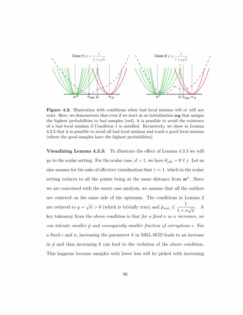
Figure 4.2: Illustration with conditions when bad local minima will or will notexist. Here, we demonstrate that even if we start at an initialization wB that assignsthe highest probabilities to bad samples (red), it is possible to avoid the existenceof a bad local minima if Condition 1 is satisfied. Recursively, we show in Lemma4.3.3 that it is possible to avoid all bad local minima and reach a good local minima(where the good samples have the highest probabilities)
Visualizing Lemma 4.3.3: To illustrate the effect of Lemma 4.3.3 we will
go to the scalar setting. For the scalar case, d = 1, we have θj,w = 0 ∀ j. Let us
also assume for the sake of effective visualization that γ = 1, which in the scalar
setting reduces to all the points being at the same distance from w∗. Since
we are concerned with the worst case analysis, we assume that all the outliers
are centered on the same side of the optimum. The conditions in Lemma 2
are reduced to q =√κ > 0 (which is trivially true) and pmax ≤
1
1 + κ√κ
. A
key takeaway from the above condition is that for a fixed n as κ increases, we
can tolerate smaller p and consequently smaller fraction of corruptions ε. For
a fixed ε and n, increasing the parameter k in MKL-SGD leads to an increase
in p and thus increasing k can lead to the violation of the above condition.
This happens because samples with lower loss will be picked with increasing
86

probability as k increases.
Let wMKL be the stationary point of MKL-SGD for this scalar case. If
the above condition is satisfied, then the existence of the first bad MKL-SGD
stationary point wMKL can be avoided as illustrated in Figure 4.2.
To further elaborate on this, let us initialize MKL-SGD at w0 = wB,
a point where the losses of outlier samples are 0 and all the clean samples
have non-zero losses. If C1 holds true, then we are in Case 1 (Figure 4.2),
the stationary point attained by MKL-SGD will be such that it is possible
to avoid the existence of the first bad local minima which occurs when the
top-|O| highest probabilities are assigned to the bad samples.
Not only that all other subsequent local minimas are avoided as well,
until we reach the local minima which assigns the largest (n−|O|) probabilities
to the clean samples1. This indicates that irrespective of where we initialize in
the 1D landscape, we are bound to end up at a local minima with the highest
probabilities assigned to the clean samples. In the latter part of this section,
we will show that MKL-SGD solution attained when Case 1 holds is provably
better than the SGD solution. However, if condition 1 is false (Case 2, Figure
4.2), then it is possible that MKL-SGD gets stuck at any one of the many local
minimas that exist close to the outlier center wB and we cannot say anything
about the relative distance from w∗.
1Refer to Appendix section ?? for further details on this discussion
87

Analysis for the general outlier setting: In this part, we analyze the
fixed point equations associated with MKL-SGD and SGD and try to under-
stand the behavior in a ball Br(w∗) around the optimum? For the sake of
simplicity, we will assume that ‖∇fi(w)‖ ≤ G ∀ i ∈ O. Next, we analyze the
following two quantities: i) distance of wSGD from w∗ and distance of the any
of the solutions attained by wMKL from w∗.
Lemma 4.3.4. Let wSGD indicate the solution attained SGD. Under assump-
tions 1-3, there exists an ε′ such that for all ε ≤ ε′,
εG ≤ (1− ε)L‖wSGD −w∗‖
Using Lemma 4.3.1, we will define λ as follows:
λ := minw
λw (4.7)
Assumption 2 ensures that λ > 0, however the lower bounds for this λ are
loss function dependent.
Lemma 4.3.5. Let wMKL be any first order stationary point attained by
MKL-SGD . Under assumptions 1-3, for a given ε < 1 and λ as defined in
equation (4.7), there exists a k′ such that for all k ≥ k′,
‖wMKL −w∗‖ ≤εkG
λ
Finally, we show that any solution attained by MKL-SGD is provably
better than the solution attained by SGD. We would like to emphasize that this
88
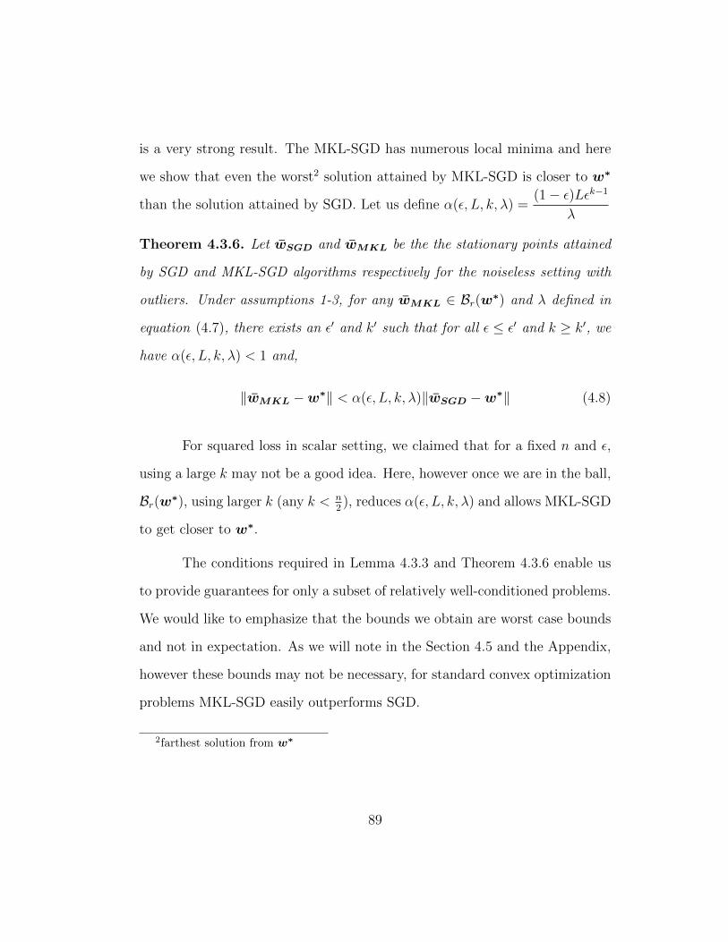
is a very strong result. The MKL-SGD has numerous local minima and here
we show that even the worst2 solution attained by MKL-SGD is closer to w∗
than the solution attained by SGD. Let us define α(ε, L, k, λ) =(1− ε)Lεk−1
λ
Theorem 4.3.6. Let wSGD and wMKL be the the stationary points attained
by SGD and MKL-SGD algorithms respectively for the noiseless setting with
outliers. Under assumptions 1-3, for any wMKL ∈ Br(w∗) and λ defined in
equation (4.7), there exists an ε′ and k′ such that for all ε ≤ ε′ and k ≥ k′, we
have α(ε, L, k, λ) < 1 and,
‖wMKL −w∗‖ < α(ε, L, k, λ)‖wSGD −w∗‖ (4.8)
For squared loss in scalar setting, we claimed that for a fixed n and ε,
using a large k may not be a good idea. Here, however once we are in the ball,
Br(w∗), using larger k (any k < n2), reduces α(ε, L, k, λ) and allows MKL-SGD
to get closer to w∗.
The conditions required in Lemma 4.3.3 and Theorem 4.3.6 enable us
to provide guarantees for only a subset of relatively well-conditioned problems.
We would like to emphasize that the bounds we obtain are worst case bounds
and not in expectation. As we will note in the Section 4.5 and the Appendix,
however these bounds may not be necessary, for standard convex optimization
problems MKL-SGD easily outperforms SGD.
2farthest solution from w∗
89

4.4 Convergence Rates
In this section, we go back to the usual in expectation convergence
analysis for the stochastic setting. For smooth functions with strong convex-
ity, [91, 90] provided guarantees for linear rate of convergence. We restate
the theorem here and show that the theorem still holds for the non-convex
landscape obtained by MKL-SGD in noiseless setting.
Lemma 4.4.1 (Linear Convergence [90]). Let F (w) = E[fi(w)] be λ-
strongly convex. Set σ2 = E[‖∇fi(w∗)‖2] with w∗ := argminF (w). Suppose
η ≤ 1supi Li
. Let ∆t = wt −w∗. After T iterations, SGD satisfies:
E[‖∆T‖2
]≤ (1− 2ηC)T‖∆0‖2 +Rσ (4.9)
where C = λ(1− η supi Li) and Rσ = ησ2
C.
In the noiseless setting, we have ‖∇fi(w∗)‖ = 0 and so σ := 0. w∗ in
(4.9) is the same as w∗ stated in Theorem 4.3.2. Even though above theorem
is for SGD, it still can be applied to our algorithm 2. At each iteration there
exists a parameter λwt that could be seen as the strong convexity parameter
(c.f. Lemma 4.3.1). For MKL-SGD, the parameter λ in (4.9) should be λ =
mint λwt . Thus, MKL-SGD algorithm still guarantees linear convergence result
but with an implication of slower speed of convergence than standard SGD.
However, Lemma 4.4.1 will not hold for MKL-SGD in noisy setting
since there exists no strong convexity parameter. Even for noiseless setting,
the rate of convergence for MKL-SGD given in Lemma 4.4.1 is not tight.
90

The upper bound in (4.9) is loosely set to the constant λ := mint λwt for
all the iterations. We fix it by concretely looking at each iteration using the
following notation. Denote the strong convexity parameter λgood for all the
good samples. Let
ψ = 2ηtλgood(1− ηt supiLi)
n− |O|ψn
.
Next, we give a general bound for the any stochastic algorithm (c.f. Theorem
4.4.2) for both noiseless and noisy setting in absence and presence of outliers.
Theorem 4.4.2 (Distance to w∗). Let ∆t = wt − w∗. Suppose at tth
iteration, the stepsize is set as ηt, then conditioned on the current parameter
wt, the expectation of the distance between the wt+1 and w∗ can be upper
bounded as:
Ei[‖∆t+1‖2|wt
]≤ (1− ψ) ‖∆t‖2 + ηtRt (4.10)
where
Rt =− ψ∑i/∈O
Npi(wt)− 1
N − |O| 〈∆t,∇fi(wt)−∇fi(w∗)〉
+ 2∑i/∈O
pi(wt)(ηt‖∇fi(w∗)‖2 − 〈∆t,∇fi(w∗)〉
)+∑i∈O
pi(wt)(ηt‖∇fi(wt)‖2 + (fi(w
∗)− fi(wt)))
Theorem 4.4.2 implies that for any stochastic algorithm in the both
noisy and noiseless setting, outliers can make the upper bound (Rt) much
worse as it produces an extra term (the third term in Rt). The third term
in Rt has a lower bound that is an increasing function of |O|. However, its
91

impact can be reduced by appropriately setting pi(wt), for instance using a
larger k in MKL-SGD . In the appendix, we also provide a sufficient condition
(Corollary 1 in the Appendix) when MKL-SGD is always better than standard
SGD (in terms of its distance from w∗ in expectation).
4.5 Experiments
In this section, we compare the performance of MKL-SGD and SGD
for synthetic datasets for linear regression and small-scale neural networks.
4.5.1 Linear Regression
For simple linear regression, we assume that Xi are sampled from nor-
mal distribution with different condition numbers. Xi ∼ N (0,D) where D
is a diagonal matrix such that D11 = κ and Dii = 1 for all i). We compare
the performance of MKL-SGD and SGD for different values of κ (Fig. 4.3)
under noiseless and noisy settings against varying levels of corruption ε. It
is important to note that different κ values correspond to different rates of
convergence. To ensure fair comparison, we run the algorithms till the error
values stop decaying and take the distance of w∗ from the exponential moving
average of the iterates.
4.5.2 Neural Networks
For deep learning experiments, our results are in presence of corruptions
via the directed noise model. In this corruption model, all the samples of class
92

0.1 0.2 0.3 0.4ε
10−4
10−3
10−2
10−1
100
||w−
w∗ ||
2
Noiseless linear regression with outliers, d = 25
MKL (κ=15)MKL (κ=10)MKL (κ=5)MKL (κ=1)SGD (κ=15)SGD (κ=10)SGD (κ=5)SGD (κ=1)
0.1 0.2 0.3 0.4ε
1
2
3
4
5
6
7
||w−
w∗ ||
2
Noisy linear regression with outliers, d = 25, σnoise = 1
MKL (κ=15)MKL (κ=10)MKL (κ=5)MKL (κ=1)SGD (κ=15)SGD (κ=10)SGD (κ=5)SGD (κ=1)
Figure 4.3: Comparing the performance of MKL-SGD (k = 2) and SGD fordifferent values of κ in noiseless and noisy linear regression against varying fractionof outliers.
93

a that are in error are assigned the same wrong label b. This is a stronger
corruption model than corruption by random noise (results in Appendix). For
the MKL-SGD algorithm, we run a more practical batched (size b) variant such
that if k = 2 the algorithm picks b/2 samples out of b sample loss evaluations.
The oracle contains results obtained by running SGD over only non-corrupted
samples.
MNIST: We train standard 2 layer convolutional network on subsampled
MNIST (5000 samples with labels). We train over 80 epochs using an initial
learning rate of 0.05 with the decaying schedule of factor 5 after every 30
epochs. The results of the MNIST dataset are averaged over 5 runs.
Dataset MNISTε\ Optimizer SGD MKL-SGD Oracle0.1 96.76 96.49 98.520.2 92.54 95.76 98.330.3 85.77 95.96 98.160.4 71.95 94.20 97.98
Table 4.1: Comparing the test accuracy of SGD and MKL-SGD (k = 5/3) overMNIST dataset in presence of corruptions via directed label noise.
CIFAR10: We train Resnet-18 [113] on CIFAR-10 (50000 training samples
with labels) for over 200 epochs using an initial learning rate of 0.05 with the
decaying schedule of factor 5 after every 90 epochs. The reported accuracy
94

is based on the true validation set. The results of the CIFAR-10 dataset are
averaged over 3 runs.
Dataset CIFAR10ε\ Optimizer SGD MKL-SGD Oracle0.1 79.1 81.94 84.560.2 72.29 77.77 84.400.3 63.96 66.49 84.660.4 52.4 53.57 84.42
Table 4.2: Comparing the test accuracy of SGD and MKL-SGD (k = 5/3) overCIFAR-10 dataset in presence of corruptions via directed label noise.
Further experimental results on random noise as well as directed noise
are available in the Appendix.
4.6 Discussion and Future Work
To ensure consistency, i.e. ‖wMKL − w∗‖ → 0, we require that
k ≥ nε + 1. In all other cases, there will be a non-zero contribution from
the outliers which keeps the MKL-SGD solution from exactly converging to
w∗. In this paper, we consider unknown ε and thus k should be a hyperparam-
eter. For neural network experiments in the Appendix, we show that tuning k
as a hyperparameter can lead to significant improvements in performance in
presence of outliers.
The obvious question is if it is possible to provide worst case guarantees
for a larger subset of problems using smarter initialization techniques. It will
95

0 50 100 150Epochs
10−5
10−4
10−3
10−2
10−1
100
Loss
Training loss
Min-2 Loss SGDSGD
0 50 100 150Epochs
1.2
1.4
1.6
1.8
2.0
2.2
2.4
2.6
2.8
Loss
Test loss
Min-2 Loss SGDSGD
0 50 100 150Epochs
40
50
60
70
80
Acc
urac
y
Test Accuracy
Min-2 Loss SGDSGD
Figure 4.4: Comparing training loss, test loss and test accuracy of MKL-SGD andSGD. Parameters: ε = 0.2, k = 2, b = 16. The training loss is lower for SGD whichmeans that SGD overfits to the noisy data. The lower test loss and higher accuracydemonstrates the robustness MKL-SGD provides for corrupted data.
be interesting to analyze the tradeoff between better generalization guarantees
offered by large k and rates of convergence. The worst case analysis in the
noisy setting for standard convex optimization losses remains an open problem.
As we show in the previous set of experiments, in presence of noise, tuning the
hyperparameter k can provide significant boosts to the performance.
96

4.7 Conclusion
In this paper, we propose MKL-SGD that is computationally inex-
pensive, has linear convergence (upto a certain neighborhood) and is robust
against outliers. We analyze MKL-SGD algorithm under noiseless and noisy
settings with and without outliers. MKL-SGD outperforms SGD in terms
of generalization for both linear regression and neural network experiments.
MKL-SGD opens up a plethora of challenging questions with respect to un-
derstanding convex optimization in a non-convex landscape which will be dis-
cussed in the Appendix.
97

Chapter 5
Balancing SGD: Faster Optimization for
Imbalanced Classification
A classification dataset is imbalanced if the number of training samples
in each class varies widely. In such a setup, vanilla SGD quickly reaches a
point where many samples from the majority class have small gradients and
low loss, leading to insignificant gradients, which in turn leads to both slow
convergence and poor generalization. In this paper, we propose a simple yet
efficient variant of SGD that rejects samples from the majority class unless
their current loss exceeds a threshold. We prove that this algorithm converges
at a faster rate than vanilla SGD and has better generalization performance.
Finally, we also illustrate these performance improvements via experiments on
synthetic as well as real datasets.
5.1 Introduction
This paper focuses on multi-class classification settings where the train-
ing data is imbalanced (i.e., it has many more samples from some classes than
from others). For a classification model trained by an algorithm like SGD,
imbalanced datasets result in two issues: slow convergence during training,
98

and final classifiers that are biased against minority classes. As we will see,
slow convergence arises because, when SGD samples are chosen uniformly at
random, most samples from the majority class have relatively small gradients
and contribute minimally to the magnitude of the update – effectively wasting
computation. On the other hand, bias – which results in poor generalization
if the test set is not imbalanced – is a result of the majority class being over-
represented in the loss function, if such a function is built naively from the
training data.
Figure 5.1: Illustration of how a skewed data distribution introduces a bias inclassical estimation techniques. w∗ determines the direction of the separating hy-perplane in presence of balanced data, and w is the predicted estimator using SGDin presence of imbalanced data.
Our primary contribution is a simple modification of SGD, which alle-
viates both issues. Our main idea is to have class-dependent thresholds on
the (current) loss of a sample – such that any randomly drawn sample not
99

meeting the threshold corresponding to its class is not used for the gradient
update.
In Figure 5.1, we highlight how the presence of imbalancedness leads
to a biased estimation using a toy example for binary classification under the
separable data regime. As the level of imbalancedness increases, the naive
optimization algorithm converges to a point farther from the desired solution
[114, 115]. A-priori knowledge of the label/data distribution can reduce the
bias and ameliorate the generalization performance [11]. Label-distribution
aware variants of SGD are quite popular [116, 12]. However, for massive
datasets, knowledge of label distribution knowledge is often unavailable, and
estimates for label distribution can be computationally challenging and in-
tractable in the stochastic setting.
Figure 5.2: Toy example for logistic regression in the separable data setting. Weplot the running average of the norm of the gradients vs. the number of samplesof that class observed when the imbalance ratio is 0.01. The window size for therunning average is 20. Samples from the majority class have insignificant gradientupdates using SGD.
100

In Figure 5.2, we use a toy example for logistic regression to draw
a comparison between the gradient contributions by the majority class and
minority class. The presence of imbalancedness (as depicted in Figure 5.1)
often biases the estimator w away from w∗. It is well known that the loss and
the norm of the gradient of a data sample i are inversely proportional to its
distance from w. Thus, for any classical method such as SGD, most samples
from the majority class have small gradients leading to many insignificant
gradient update steps, even though the optimization is far from complete.
Thus, the presence of bias not only contributes to poor generalization on the
test set but also to slow convergence. For the separable regime, under certain
assumptions, [117, 118] explicitly characterize this slow rate of convergence to
be O (1/log t) for the bias term and O (1/(log t)2) for the direction.
In recent years, some papers have systematically studied the theory
behind optimization algorithms, where samples from different classes have
different relative importance. Amongst the ones that are closely related to
our paper are Perceptron Algorithm with Uneven Margins (PAUM) in [114],
DM-SGD in [119] and Instance Shrinking in [120]. However, [114] holds for
the deterministic setting, and [119, 120] have to be significantly altered in
the presence of imbalancedness. We aim to bridge the gap between theory
and practice by providing a faster algorithm for stochastic optimization in
imbalanced classification.
101

Main Contributions
i) We propose a simple, efficient, practical variant of SGD, called Balancing
SGD (B-SGD) algorithm. This algorithm performs a gradient update step if
the loss of an incoming data sample exceeds a class-dependent threshold. This
allows B-SGD to handle the trade-off between overfitting to the majority and
overfitting to the minority class in a principled manner.
ii) We provide two main theoretical results. In Theorem 1, we provide a thresh-
old dependent upper bound on the number of gradient updates performed by
B-SGD. Next, we propose a technique to choose the class-dependent threshold
in the absence of the knowledge of label/data distributions.
iii) Lastly, we support our theoretical results with both synthetic logistic re-
gression experiments that provide insight, as well as encouraging results on real
imbalanced logistic regression and artificially generated imbalanced CIFAR-10.
5.2 Related Work
In the last few years, imbalanced learning has received considerable
interest in the machine learning community [121, 116, 122, 123, 124]. The
algorithms designed to cater to imbalanced data have one underlying theme:
design a proxy distribution that is closer in expectation to the test-set distri-
bution. These algorithms fall into the following categories:
Oversampling. Oversampling is one of the most popular choices within
the family of resampling strategies. Here, the main idea is simple: reuse the
samples of the minority class by resampling them. Naive over-sampling of the
102

minority class does not lead to improvements in performance [125, 126, 9].
Popular variants of over-sampling include either reweighting the existing ex-
amples based on some criteria [10] or creating synthetic examples [9]. However,
over-sampling variants often suffer from overfitting to minority class [127, 128]
and so require regularization methods [129], which might result in significant
memory requirements, poor performance on high-dimensional data [130] and
slow convergence. The last point arises from the fact that as the number of
samples increases, it lowers the relative importance of each sample [131].
Undersampling. Undersampling relies on the idea of removing the sam-
ples of the majority class to balance the distribution. Under-sampling meth-
ods [132, 127, 122] can often lead to the loss of crucial information about
the estimator [11] if performed arbitrarily. Moreover, without knowing the
data-distribution [12], determining the extent of resampling further affects the
final performance. For large datasets, it becomes crucial as it is expensive to
compute and store these statistics.
Loss-based classification. Loss-based classification (or Cost-sensitive
learning) is another widely used approach to balance the distributions. Over
the years, variants of cost-sensitive algorithms have been proposed such as
MFE and MSFE loss [133], Focal Loss [2, 134], CSDNN [135], CoSen CNN
[136], CSDBN-DE [137], Threshold moving [138, 116] and many others [139,
140, 141, 131, 142].
Ensemble methods. In ensemble learning, a combination of the above
methods can be tailored to improve the performance for specific applications
103

[138, 143, 144, 145, 146]. [147, 148] provide a detailed comparison of various
methods for imbalanced learning. However, most of the techniques require the
knowledge of label distribution, limiting their applicability in the stochastic
setting.
To alleviate these issues in imbalanced learning, we propose an algo-
rithm called Balancing SGD (B-SGD), which decides on the fly whether to
compute a gradient update according to the estimated imbalance ratio, as
well as the label and loss value of the incoming data sample. We observe
that by combining resampling strategies with cost-sensitive learning, we can
improve the convergence rates on imbalanced datasets than SGD and other
methods that are agnostic of the label distribution.
Algorithm 3 Balancing SGD (B-SGD)
1: Number of classes k; Threshold parameter c > 0; Threshold values τ =[τi], i ∈ [k].
2: Initialize w0, τi(0) = τi, nyi = 0 ∀ i ∈ [k]3: Given samples S = (xi, yi)
∞i=1
4: for t = 1, 2, 3, . . . T do5: Choose a sample i uniformly from S6: if fi(wt) ≥ τyi(t) then7: wt+1 = wt − η∇fi(wt)8: nyi = nyi + 1
9: τyi(t+ 1) = c
(k−1k−
∑j∈j∈[k]|yj 6=yi
nyj∑j∈[k] nyj
)10: else11: wt+1 = wt, τyi(t+ 1) = τyi(t)12: end if13: τyj(t+ 1) = τyj(t) ∀ j 6= i14: end for15: Return wT
104

5.3 Algorithm
We propose a simple variant of SGD, known as the Balancing-SGD (B-
SGD) algorithm to improve both the generalization and convergence behavior
of SGD: in each step, calculate the loss of the incoming sample fi(wt), and
perform a gradient update step for that sample if it exceeds the label-dependent
loss threshold, τyi(t). In other words, let Tt ∈ S indicate the set of samples
in the training set S that satisfy the label-dependent loss threshold condition,
i.e., Tt := i ∈ S|fi(wt) ≥ τyi(t).
The effective gradient update for B-SGD is then given as follows:
E [wt+1|wt] = wt − η∇fi(wt)Ii∈Tt
Here, Tt is a dynamic set that can contain anywhere from 0 data samples to
all data samples in S depending on the value of wt and τyi(t). The rejection
of samples that have a low loss with a time-varying label-dependent threshold
result in a dynamically changing loss function similar to [149].
Line 9 is the critical part of Algorithm 3, which describes the loss
threshold selection process. While we elaborate on how threshold selection
happens later in Section 5.4.4, let us motivate why Line 9 is helpful. i) If
the number of gradient updates for all the classes is the same, then the loss
threshold is zero for all classes. Thus, in the presence of a balanced training set,
B-SGD mimics SGD. ii) The loss threshold should be inversely proportional
to the number of gradient updates for samples of that class, i.e., larger the
number of gradient updates for that class, higher should be the loss threshold.
105

iii) Let nm and nM be the number of gradient update steps taken for classes
1 and 2, respectively. For a simple setting with k = 2 classes and n1 < n2,
we have τ1 = c(0.5 − n2
n1) > 0, τm = c(0.5 − n2
n1) < 0 which passes the sanity
check of selectively choosing samples from the majority class. iv) Note, that
the threshold expression acts as a self-adjusting function, i.e. if fewer samples
from a class i are selected, it leads to a reduction in the value of τyi which in
turn decreases the probability of rejection for a sample belonging to class i in
future updates.
Thus, B-SGD takes gradient update steps more frugally than SGD. In
practice, this is particularly important as computing gradients are usually more
expensive than computing the loss functions for a given sample. For example,
in deep learning, loss calculations often involve just forward propagation, while
gradient computations involve both forward and backward propagation.
The algorithm exhibits two key features:
i. Boosting-like updates [150]: Update samples with higher loss more fre-
quently than corresponding samples with the lower loss
ii. Passive-aggressive updates [151, 152, 153]: τyi(t) is inversely proportional
to the frequency of the gradient update step taken for each class, i.e.,
majority class will have a higher loss threshold τyi(t) than the minority
class
The B-SGD algorithm requires O(k) extra memory, where k is the
106

Figure 5.3: Introducing a label-dependent loss-based thresholding approach allowsus to alleviate the issue of bias introduced by the skewed label distribution
number of classes. The computational complexity of the B-SGD algorithm is
the same as SGD; O(1) gradient/loss computations per incoming sample.
B-SGD belongs to the class of ensemble methods that combine under-
sampling and loss-based classification. It is important to note that while the
undersampling for the majority class can include any subset of points, i.e., the
ones with high loss, those with low loss, or those within some range of loss
values. Here, the choice of the subset with high loss has twofold advantages: i)
fewer gradient computations, ii) the information about support vectors which
determine the separating hyper-plane is not lost.
We reiterate that similar approaches have been utilized in literature
with limited success. These approaches suffer from many issues, such as cater-
ing to specific applications, expensive pre-computations, access to label dis-
107

tribution, and slow convergence in the stochastic setting. With B-SGD, we
propose a systematic approach to alleviate these issues in imbalanced classifi-
cation.
5.4 Theoretical Results for Logistic Regression
Notation: Throughout, ‖ · ‖ denotes the Euclidean `2 norm. D is the
unknown distribution of the data set and S is the training data such that
|S| = n. Bold-faced lowercase letters will be used to denote vectors while plain
lowercase letters indicate scalars. Without loss of generality, we also assume
that the data is imbalanced with y = 1 denoting the minority class. S−1 and
S1 represent the training data for majority class (y = −1) and minority class
(y = 1) respectively. Let the imbalance ratio be denoted by r = # of (+1)′sn
.
The function h(s) : R → R is an decreasing function of s. σ(q) = 11+exp(−q)
denotes the sigmoid function. w∗ is the optimal solution for LD(w).
5.4.1 System Model
For any dataset S := xi, yini=1 with features xi ∈ Rd and labels yi ∈
R, the corresponding empirical risk S minimization problem can be formulated
as:
minw
LS(w) where LS(w) =1
n
n∑i∈S
fi(w) (5.1)
Here, fi(w) := f(w; (xi, yi)) represent convex, continuously differentiable loss
functions for the sample (xi, yi). Similarly, the population risk minimization
108

is expressed as follows:
minwLD(w) where LD(w) := Ei∼D[fi(w)] (5.2)
Our aim is to use S to find an estimator that minimizes the population risk
in equation (5.2). In the rest of this section, we focus on binary classification
of imbalanced datasets using logistic regression.
Definition 5.4.1 (Linearly separable). For the generative logistic model, the
underlying parameter w∗ ∈ Rd+1 determines the separating hyperplane where
w∗ is defined as:
w∗ = [(w∗(d))> b∗]
> ∈ Rd+1, where w∗(d)/‖w∗(d)‖ is direction and b∗is bias.
(5.3)
The class for the input feature x(d) in D is determined as follows:
x = [(x(d))> 1]> ∈ Rd+1, y = 1σ(w∗>x) ≥ 0.5 − 1σ(w∗
>x) < 0.5(5.4)
where (d+ 1)th dimension is for the constant term and σ(x) = 1/(1 + e−x).
The deterministic generative process in equation (5.4) ensures that our
training samples S = xi, yini=1 are linearly separable.
The logistic loss for data sample (xi, yi) at w is given as:
fi(w) = f(w; (xi, yi)) = log(1 + exp
(−yi(w>xi)
))SGD treats all the samples in the training set equally and minimizes
the empirical objective function:
LS(w) =1
n
n∑i=1
log(1 + exp
(−yi(w>xi)
))(5.5)
109
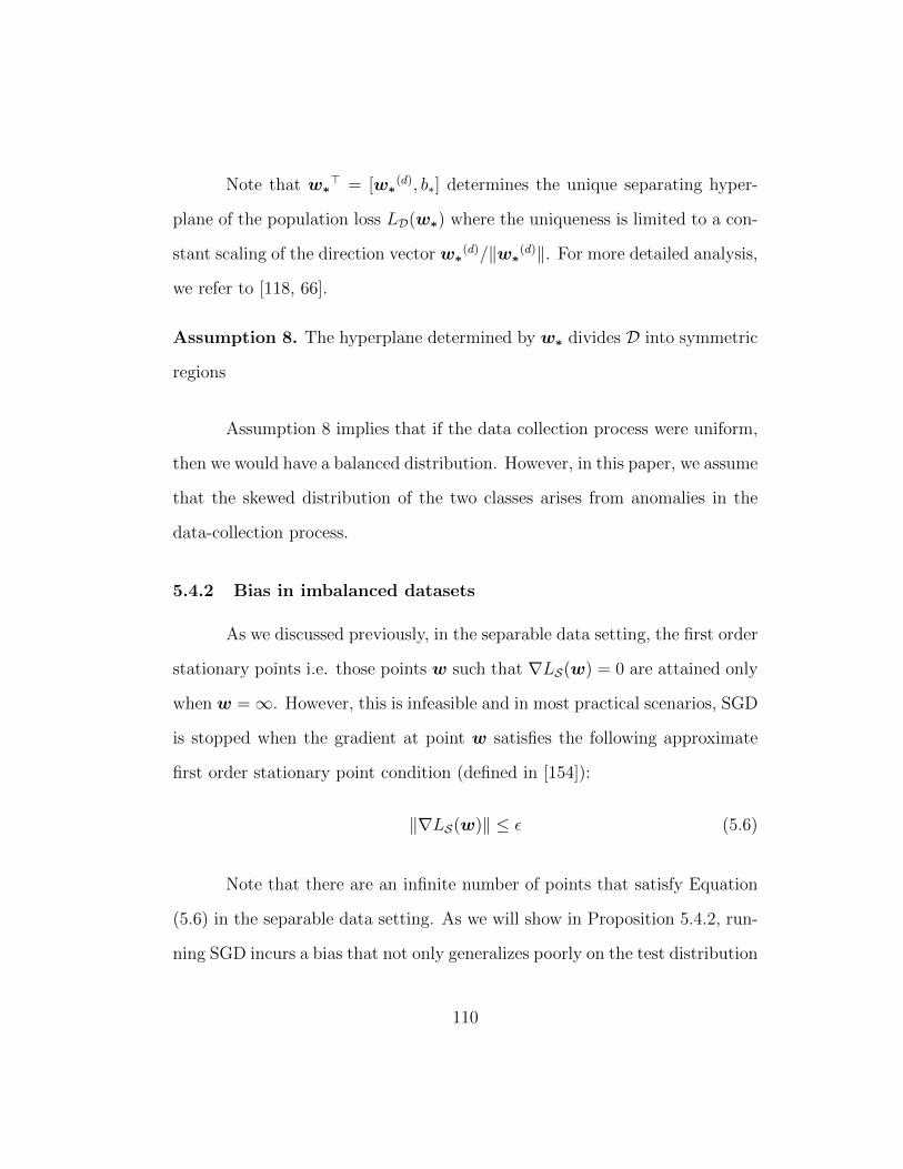
Note that w∗> = [w∗
(d), b∗] determines the unique separating hyper-
plane of the population loss LD(w∗) where the uniqueness is limited to a con-
stant scaling of the direction vector w∗(d)/‖w∗(d)‖. For more detailed analysis,
we refer to [118, 66].
Assumption 8. The hyperplane determined by w∗ divides D into symmetric
regions
Assumption 8 implies that if the data collection process were uniform,
then we would have a balanced distribution. However, in this paper, we assume
that the skewed distribution of the two classes arises from anomalies in the
data-collection process.
5.4.2 Bias in imbalanced datasets
As we discussed previously, in the separable data setting, the first order
stationary points i.e. those points w such that ∇LS(w) = 0 are attained only
when w =∞. However, this is infeasible and in most practical scenarios, SGD
is stopped when the gradient at point w satisfies the following approximate
first order stationary point condition (defined in [154]):
‖∇LS(w)‖ ≤ ε (5.6)
Note that there are an infinite number of points that satisfy Equation
(5.6) in the separable data setting. As we will show in Proposition 5.4.2, run-
ning SGD incurs a bias that not only generalizes poorly on the test distribution
110

Figure 5.4: Visualizing selection bias in imbalanced datasets using a toy example.w∗ is defined in Definition 8 and wSGD is the estimator running vanilla SGD safisfies(5.6).
D but also converges at an extremely slow rate to the maximum margin sep-
arating hyperplane of S as O (1/log t) for bias and O (1/(log t)2) for direction
[117, 118]. In the rest of this section, we will first establish the relationship be-
tween r and b (Proposition 5.4.2), and using a toy example (Fig. 5.4) establish
how high bias leads to poor convergence and generalization guarantees.
Proposition 5.4.2. Consider the loss function defined in equation (5.5) and
assume w> = [w(d), b] is an approximate stationary point satisfying equa-
tion (5.6). That is, for some |b| < ∞ and ε > 0 such that ∀i, yix>i w(d) ≥
log (1/ε) and exp(−yi(x>i w(d) + b)
)< 1. Then ∂L(w)
∂b|[]w = w = 0 implies
111

that
b ∝ log
( ∑i∈S1 e
−yix>i w(d)∑
i∈S−1e−yix
>i w
(d)
). (5.7)
Note that for Proposition 5.4.2, we do not make any specific assump-
tions and thus the bias expression holds for any w that satisfies equation (5.6).
We will utilize the toy example in Figure 5.4 to quantify the bias term. Here,
the data lies in 1-D space and satisfies Assumption 8. Let w∗ = [1, 0] and
D = (xi, yi)|xi ∈ U(−1, 1), yi = sign(xi). Consistent with our motivation
in Section 5.1, the data collection process is skewed and in the toy example
we consider an extreme case where there is only one sample in the minority
class, i.e. rn = 1, given by x1 = [x(d)1 , 1]>. Then, the number of samples in
the majority class is (1− r)n = 1−rr
where we assume that r is small (1e−3 or
less). w satisfies equation (5.6) iff b ∈ [x(d)1 , 0] where x
(d)1 < 0. Combining this
setup with equation (5.7), the bias for the toy example in Figure 5.4 can be
reduced to:
b ∝ log
(e−x
(d)i w(d)∫ 1
0ex
(d)i w(d)
dx(d)i
)≈ log
(w(d)e−x
(d)i w(d)
ew(d) − 1
).
For large values of |w(d)|, the bias tends to 0. However, for small values of |w(d)|,
however, the bias is significant. Since the test set follows the same distribution
as D i.e. is balanced, 0.5|b| fraction of samples are incorrectly classified. Thus,
larger the magnitude of |b|, higher is the generalization error of the estimator.
Further, we also show in appendix section D.2 that the bias has an impact on
the rate of convergence as well. This in turn implies that not all samples are
112

equally useful especially at low values of |w| and it can be worthwhile omitting
certain samples from the majority class S−1 in the gradient update steps to
improve both generalization and the rate of convergence.
10 2 10 1 100 101
Threshold 1
10 1
100
101 car_eval_4 dataset with r=0.037Training LossTest LossGradient computations (× 104)
Figure 5.5: Here, we compare the training error, test error and no. of gradi-ent computations for different values of fixed thresholds for the majority class. Asthreshold, τ−1, increases from 0 to 50, we observe that the no. of gradient compu-tations continues to decrease while both training and test loss initially decrease andthen increase. Advantage of fixed thresholding: B-SGD [τ−1, τ1] = [0.75, 0] achieves37.5% and 71.7% decrease in the test error and gradient computations respectivelyover SGD ( τ−1 = τ1 = 0).
113
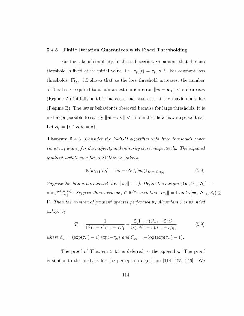
5.4.3 Finite Iteration Guarantees with Fixed Thresholding
For the sake of simplicity, in this sub-section, we assume that the loss
threshold is fixed at its initial value, i.e. τyi(t) = τyi ∀ t. For constant loss
thresholds, Fig. 5.5 shows that as the loss threshold increases, the number
of iterations required to attain an estimation error ‖w − w∗‖ < ε decreases
(Regime A) initially until it increases and saturates at the maximum value
(Regime B). The latter behavior is observed because for large thresholds, it is
no longer possible to satisfy ‖w−w∗‖ < ε no matter how may steps we take.
Let Sy = i ∈ S|yi = y,
Theorem 5.4.3. Consider the B-SGD algorithm with fixed thresholds (over
time) τ−1 and τ1 for the majority and minority class, respectively. The expected
gradient update step for B-SGD is as follows:
E [wt+1|wt] = wt − η∇fi(wt)Ifi(wt)≥τyi (5.8)
Suppose the data is normalized (i.e., ‖xi‖ = 1). Define the margin γ(w,S−1,S1) :=
miniyi(〈w,xi〉)‖w‖ . Suppose there exists w∗ ∈ Rd+1 such that ‖w∗‖ = 1 and γ(w∗,S−1,S1) ≥
Γ. Then the number of gradient updates performed by Algorithm 3 is bounded
w.h.p. by
Tτ =1
Γ2(1− r)β−1 + rβ1
+2(1− r)C−1 + 2rC1
η (Γ2(1− r)β−1 + rβ1)(5.9)
where βyi = (exp(τyi)− 1) exp(−τyi) and Cyi = − log (exp(τyi)− 1).
The proof of Theorem 5.4.3 is deferred to the appendix. The proof
is similar to the analysis for the perceptron algorithm [114, 155, 156]. We
114

adopt their ideas to our logistic regression in stochastic gradient descent for
imbalanced data and significantly improve the bounds in terms of imbalance
ratio r with high probability.
One of the main takeaways from Theorem 5.4.3 is that the number of
updates Tτ is directly determined by r. If the classes are highly imbalanced
satisfying r = O (1/ log (1/ε))), then for some ε setting τ1 = ε and τ−1 > ε
results in:
C1 = (− log(exp(ε)− 1) = O (log (1/ε)) and β1 = (exp(ε)− 1) exp(−ε) = O (ε)
which means rC1 = O(1) and rβ1 = O(ε/(log(1/ε)) have little effect on the
bound. In other words, taking all samples from highly-imbalanced minority
class will have similar sample complexity as taking a subset of samples from
the minority class with a small (constant) loss threshold. This serves as an
inspiration for our proposed Algorithm 3 in Section 5.4.4. On the other hand,
when the thresholds of both majority and minority are small (i.e., τyi → ε),
the update in (D.7) reduces to vanilla SGD, which means the bound Tτ in
Theorem 5.4.3 is: Tε = O (1/ε log (1/ε)) . The complexity Tε matches the
bound in [117]. Comparing with this vanilla SGD, Algorithm 3 with τ1 = ε
and constant τ−1 clearly achieves a smaller bound than vanilla SGD in terms of
number of gradient updates performed. In this sense, we claim Algorithm 3 has
faster optimization. Figure 5.3 provides further evidence that our algorithm
is able to achieve both good generalization as well as faster convergence over
SGD.
115

However, the B-SGD algorithm with fixed thresholds would require a
good initial estimate of r which is difficult since we do not have access to
any label or data distribution. With that in mind, in the next section, we
propose a variable thresholding approach that allows us to apply B-SGD with
an estimate Rt for imbalance ratio r based on the samples for which gradient
update steps are taken.
5.4.4 Analysis of Variable Thresholding with Unknown r
To describe the variable thresholding approach, we first delve deeper
into the analysis of stationary points for the binary classification problem. For
the separable data case, we know that there can be many separating hyper-
planes for a given set of data points, and all of them perform equally well on
the training set. However, in order to guarantee good generalization, we need
to understand why a specific solution will have better generalization. This,
in turn, motivates how we tune the threshold as we perform an increasing
number of updates.
As shown in Section 5.4.2, SGD will lead to biased estimation. However,
if we know r in advance, we minimize re-weighted empirical loss leads to an
estimator wRW that is closer to w∗ than wSGD.
wRW = arg minw
(∑i∈S1
log(1 + exp
(−w>x
))+∑i∈S−1
r
1− r log(1 + exp
(w>x
)))(5.10)
The alternative is to under-sample the majority class by removing samples to
116

have wUS as
wUS = arg minw
( ∑i∈S1∩Aw
log(
1 + exp(−w>x
))+
∑i∈S−1∩Aw
log(
1 + exp(w>x
)))(5.11)
where Aw := i ∈ S| log(1 + exp
(−yiw>x
))> τyi and τ(.) is a function of
r. We wish to find the w that satisfies equations (5.10) and (5.11), whichimplies: ∑
i∈S−1
(r
1− r − 1i∈Aw
)∇fi(w)|[
]w = w = 0 (5.12)
There exists some constant τ−1 that satisfies the equality in equation (5.12).
However, to write down the closed-form expression of τ−1 is not straightfor-
ward.
Proposition 5.4.4. Suppose the data is normalized (i.e., ‖xi‖ = 1). Suppose
w minimizes both equations (5.10) and (5.11), then without loss of generality
w>xi < 0,∀i ∈ S−1. Set τ−1 ≥ 0 for the set Aw. Solving for τ−1 given some
r in equation (5.12), we observe that τ−1 > 0 is monotonically decreasing
function with respect to r ∈ [0, 0.5]. In addition,
if r → 0.5 or r1−r → 1, then τ−1 → 0; if r → 0 or r
1−r → 0, then
τ−1 → log(1 + exp(‖w‖)).
The proof is available in the appendix. Thus, based on the Proposition
5.4.4, we propose a criteria to accept a sample from this majority class by
linearly interpolating τ−1 at r = 0 to r = 0.5:
τ−1 ≈ log(1 + exp(‖w‖))) (0.5− r) (5.13)
117

B-SGD Algorithm with unknown r: Let nmin(t) and nmaj(t) denote the
number of gradient updates for the minority and majority class respectively
at time t. Since we assume that we are not aware of the label distribution
at the start, let the running update of the parameter r denoted by Rt every
time a gradient update is performed, i.e., Rt =nmin,t
nmin,t+nmaj,twhich represents
an empirical estimate of the imbalance ratio observed so far (w.r.t. gradient
update steps). The loss threshold vector, τ , in Line 9 of Algorithm 3 becomes:
τ−1(t) = log(1 + exp(‖w‖))) (0.5−Rt)
τ1(t) = log(1 + exp(‖w‖))) (Rt − 0.5)
where Rt = nmin,t/(nmin,t + nmaj,t). This implies that for any binary classifi-
cation problem, at any point of time exactly one class can have a positive loss
threshold.
5.5 Experiments
In this section, we compare B-SGD and SGD for two different scenarios:
5.5.1 Synthetic experiments
For this subsection, we consider a generative model in the separable
setting as described in Definition 5.4.1. We compare the performance of SGD
and B-SGD, where we plot both estimation error vs. the number of gradient
computations and estimation error, ‖w − w∗‖ vs. time taken. We observe
that B-SGD outperforms SGD in the number of gradient computations and
118
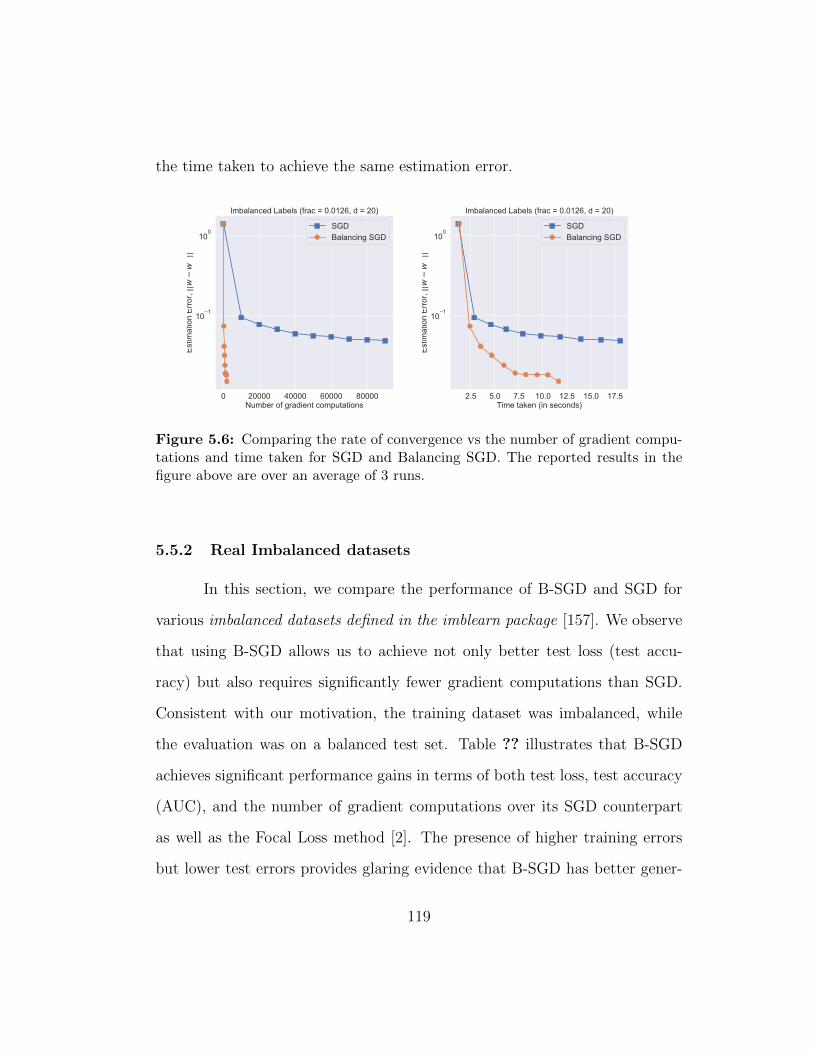
the time taken to achieve the same estimation error.
0 20000 40000 60000 80000Number of gradient computations
101
100
Est
imat
ion
Err
or, |
|ww
* ||
Imbalanced Labels (frac = 0.0126, d = 20)
SGDBalancing SGD
2.5 5.0 7.5 10.0 12.5 15.0 17.5Time taken (in seconds)
101
100
Est
imat
ion
Err
or, |
|ww
* ||
Imbalanced Labels (frac = 0.0126, d = 20)
SGDBalancing SGD
Figure 5.6: Comparing the rate of convergence vs the number of gradient compu-tations and time taken for SGD and Balancing SGD. The reported results in thefigure above are over an average of 3 runs.
5.5.2 Real Imbalanced datasets
In this section, we compare the performance of B-SGD and SGD for
various imbalanced datasets defined in the imblearn package [157]. We observe
that using B-SGD allows us to achieve not only better test loss (test accu-
racy) but also requires significantly fewer gradient computations than SGD.
Consistent with our motivation, the training dataset was imbalanced, while
the evaluation was on a balanced test set. Table ?? illustrates that B-SGD
achieves significant performance gains in terms of both test loss, test accuracy
(AUC), and the number of gradient computations over its SGD counterpart
as well as the Focal Loss method [2]. The presence of higher training errors
but lower test errors provides glaring evidence that B-SGD has better gener-
119
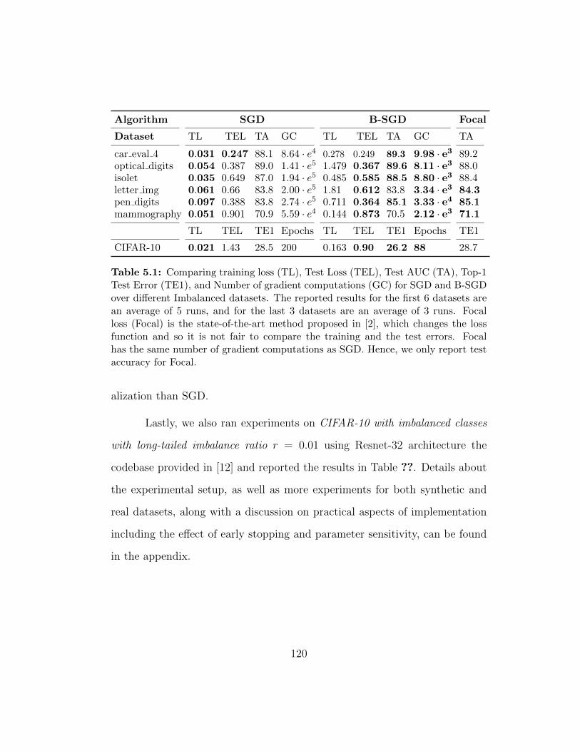
Algorithm SGD B-SGD Focal
Dataset TL TEL TA GC TL TEL TA GC TA
car eval 4 0.031 0.247 88.1 8.64 · e4 0.278 0.249 89.3 9.98 · e3 89.2optical digits 0.054 0.387 89.0 1.41 · e5 1.479 0.367 89.6 8.11 · e3 88.0isolet 0.035 0.649 87.0 1.94 · e5 0.485 0.585 88.5 8.80 · e3 88.4letter img 0.061 0.66 83.8 2.00 · e5 1.81 0.612 83.8 3.34 · e3 84.3pen digits 0.097 0.388 83.8 2.74 · e5 0.711 0.364 85.1 3.33 · e4 85.1mammography 0.051 0.901 70.9 5.59 · e4 0.144 0.873 70.5 2.12 · e3 71.1
TL TEL TE1 Epochs TL TEL TE1 Epochs TE1
CIFAR-10 0.021 1.43 28.5 200 0.163 0.90 26.2 88 28.7
Table 5.1: Comparing training loss (TL), Test Loss (TEL), Test AUC (TA), Top-1Test Error (TE1), and Number of gradient computations (GC) for SGD and B-SGDover different Imbalanced datasets. The reported results for the first 6 datasets arean average of 5 runs, and for the last 3 datasets are an average of 3 runs. Focalloss (Focal) is the state-of-the-art method proposed in [2], which changes the lossfunction and so it is not fair to compare the training and the test errors. Focalhas the same number of gradient computations as SGD. Hence, we only report testaccuracy for Focal.
alization than SGD.
Lastly, we also ran experiments on CIFAR-10 with imbalanced classes
with long-tailed imbalance ratio r = 0.01 using Resnet-32 architecture the
codebase provided in [12] and reported the results in Table ??. Details about
the experimental setup, as well as more experiments for both synthetic and
real datasets, along with a discussion on practical aspects of implementation
including the effect of early stopping and parameter sensitivity, can be found
in the appendix.
120

Appendices
121

Appendix A
Cheap-SVRG
A.1 Proof of Theorem 2.4.2
By assumptions of the theorem, we have:
η <1
4L((1 + θ) + 1
s
) and K >1
(1− θ)η (1− 4Lη) γ,
As mentioned in the remarks of Section 2.4, the above conditions are sufficient
to guarantee ρ < 1, for some θ ∈ (0, 1). Further, for given accuracy parameter
ε, we assume κ ≤ ε2.
Let us define
ϕt := E[F (wt)− F (w∗)
],
as in the proof of Theorem 2.4.1. In order to satisfy varphiT ≤ ε, it is sufficient
to find the required number of iterations such that ρTϕ0 ≤ ε2. In particular:
ρTϕ0 ≤ε
2⇒ − (T log ρ+ logϕ0) ≥ − log
ε
2
⇒ T · log(ρ−1)≥ log
2
ε+ logϕ0
⇒ T ≥(
log1
ρ
)−1
· log
(2 (F (w0)− F (w∗))
ε
)
122

Moreover, each epoch involves K iterations in the inner loop. Each inner loop
iteration involves two atomic gradient calculations. Combining the above, we
conclude that the total number of gradient computations required to ensure
that ϕT ≤ ε is O((2K + s) log 1
ε
).
A.2 Mini-batches in CheapSVRG
In the sequel, we show how Alg. 1 can also accommodate mini-batches
in the inner loops and maintain similar convergence guarantees, under As-
sumptions 1-4. The resulting algorithm is described in Alg. 4. In particular:
Algorithm 4 CheapSVRG with mini batches
1: Input: w0, η, s, q,K, T .2: Output: wT .3: for t = 1, 2, . . . , T do4: Randomly select St ⊂ [n] with cardinality s.5: Set w = wt−1 and S = St.6: µS = 1
s
∑i∈S ∇fi(w).
7: w0 = w.8: for k = 1, . . . , K − 1 do9: Randomly select Qk ⊂ [n] with cardinality q.
10: Set Q = Qk.11: vk = ∇fQ(wk−1)−∇fQ(w) + µS .12: wk = wk−1 − η · vk.13: end for14: wt = 1
K
∑K−1j=0 wj.
15: end for
Theorem A.2.1 (Iteration invariant). Let w∗ be the optimal solution for
minimization (2.1). Further, let s, q, η, T and K be user defined parameters
123

such that
ρdef=
q
η · (q − 4L · η) ·K · γ +4L · η · (s+ q)
(q − 4L · η) · s < 1.
Under Asm. 1-4, CheapSVRG satisfies the following:
E[F (wT )− F (w∗)
]≤ ρT · (F (w0)− F (w∗))
+q
q − 4Lη·(
2η
s+
ζ
K
)·max
ξ, ξ2
· 1
1− ρ.
A.3 Proof of Theorem A.2.1
To prove A.2.1, we analyze CheapSVRG starting from its core inner
loop (Lines 9-14). We consider a fixed subset S ⊆ [n] and show that in
expectation, the steps of the inner loop make progress towards the optimum
point. Then, we move outwords to the ‘wrapping’ loop that defines consecutive
epochs to incorporate the randomness in selecting the set S.
We consider the kth iteration of the inner loop, during the tth iteration
of the outer loop; we consider a fixed set S ⊆ [n], starting point w0 ∈ Rp and
(partial) gradient information µS ∈ Rp as defined in Steps 6−8 of Alg. 1. The
set Qk is randomly selected from [n] with cardinality |Qk| = q. Similarly to
the proof of Thm. 2.4.1, we have:
EQk[‖wk −w∗‖2
2
]= ‖wk−1 −w∗‖2
2 − 2η · (wk−1 −w∗)> EQk [vk]
+ η2EQk[‖vk‖2
2
]. (A.1)
where the expectation is with respect to the random variable Qk. By the
124

definition of vk in Line 12,
EQk [vk] = EQk [∇fQk(wk−1)−∇fQk(w) + µS ]
= ∇F (wk−1)−∇F (w) + µS , (A.2)
where the second step follows from the fact that Qk is selected uniformly at
random from [n]. Similarly,
EQk[‖vk‖2
2
]= EQk
[‖∇fQk(wk−1)−∇fQk(w) + µS‖2
2
](i)
≤ 4 · EQk[‖∇fQk(wk−1)−∇fQk(w∗)‖2
2
]+ 4 · EQk
[‖∇fQk(w)−∇fQk(w∗)‖2
2
]+ 2 · ‖µS‖2
2
(ii)
≤ 8L
q· (F (wk−1)− F (w∗) + F (w)− F (w∗)) + 2 · ‖µS‖2
2.
(A.3)
Inequality (i) is follows by applying ‖x − y‖22 ≤ 2‖x‖2
2 + 2‖y‖22 on all atomic
gradients indexed by Qk, while (ii) is due to the following lemma.
Lemma A.3.1. Given putative solution wk−1 and mini-batch Qk with cardi-
nality |Qk| = q, the following holds true on expectation:
EQk[‖∇fQk(wk−1)−∇fQk(w∗)‖2
2
]≤ q−1 · 2L · (F (wk−1)− F (w∗)) .
Proof. let
Q =Qi : |Qi| = |Q|, Qi ⊂ [n], Qi 6= Qj,∀i 6= j
,
i.e., Q contains all different index sets of cardinality |Q| = q. Observe that
|Q| =(n|Q|
).Note that the set Qk randomly selected in the inner loop of Alg. 1
125

is a member of Q. Then:
EQk[‖∇fQk(wk−1)−∇fQk(w∗)‖2
2
]= E
[∥∥|Qk|−1 ·∑i∈Qk
(∇fi(wk−1)−∇fi(w∗))∥∥2
2
]=∑Qj∈Q
P[Qj] ·∥∥∥q−1 ·
∑i∈Qj
(∇fi(wk−1)−∇fi(w∗))∥∥∥2
2
(i)=∑Qj∈Q
(n
q
)−1
·∥∥∥q−1 ·
∑i∈Qj
(∇fi(wk−1)−∇fi(w∗))∥∥∥2
2
(ii)=
(n
q
)−1
· q−2 ·∑Qj∈Q
∥∥∥∑i∈Qj
(∇fi(wk−1)−∇fi(w∗))∥∥∥2
2
≤(n
q
)−1
· q−2 ·∑Qj∈Q
∑i∈Qj
∥∥(∇fi(wk−1)−∇fi(w∗))∥∥2
2.
Here, equality (i) is follows from the fact that each Qj is selected equiprobably
from the set Q. Equality (ii) is due to the fact that |Qj| = q, ∀i.
Since each set in Q has cardinality q, each data sample i ∈ [n] con-
tributes exactly(n−1q−1
)summands in the double summation above. This further
leads to:
EQk[‖∇fQk(wk−1)−∇fQk(w∗)‖2
2
]≤(n
q
)−1
· 1
q2·(n− 1
q − 1
) n∑i=1
‖∇fi(wk−1)−∇fi(w∗)‖22
≤ q−1 · n−1 ·n∑i=1
‖∇fi(wk−1)−∇fi(w∗)‖22
(i)
≤ q−1 · 2L · (F (wk−1)− F (w∗)) .
126

Inequality (i) follows from the the fact that for any w ∈ Rp [3],
1
n·
n∑i=1
‖∇fi(w)−∇fi(w∗)‖22 ≤ 2L · (F (w)− F (w∗)) . (A.4)
Similarly, for w,
EQk[‖∇fQk(wk−1)−∇fQk(w∗)‖2
2
]≤ q−1 · 2L · (F (w)− F (w∗)) . (A.5)
Using the above lemma in (A.3), the remainder of the proof follows
that of Theorem 2.4.1.
A.4 Coordinate updates in CheapSVRG
In large-scale settings, even computing estimates of the gradient, as in
stochastic gradient variants where∇fi(w) ∈ Rd, requires a lot of computations
when d is large. Under such circumstances, it might be desirable to compute
partially the estimate ∇fi(w) by focusing only on a selected subset of its
entries. This idea leads to Coordinate Descent (CD) algorithms, where even
only a single component of ∇fi(w) is updated per iteration. We refer the
reader to [] and the excellent recent survey by Stephen Wright [] for more
information about the history of CD variants.
In this section, we describe CheaperSVRG, a coordinate-descent vari-
ant of CheapSVRG. The description of CheaperSVRG is provided in Al-
gorithm 5. The only difference with CheapSVRG is that, in every inner
127

iteration, CheaperSVRG updates exclusively a randomly selected coordi-
nate of the gradient of the selected component ∇fi(·).
In this section, we introduce the following notation. Given a set B ⊂ [d],
∇Bfi(w) ∈ Rd denotes the gradient of the i-th component of f , supported on
the set B: i.e., (∇Bfi(w))Bc = 0 for Bc := [d] \ B. With a slight abuse of
notation, we will use the same notation ∇Bfi(w) to denote the information of
∇fi(w) in Rd and R|B|; the distinction will be apparent from the context. We
also use µBkS ∈ Rd to denote the restriction of µS only on indices from Bk.
Given the above, anti-gradient direction −vk is only supported on Bk.
In the special case where S ≡ [n], we have:
Eik,Bk [vk] = db· Eik
[EBk
[∇Bkfik(wk−1)−∇Bkfik(w) + µBk | ik
]](i)= d
b· Eik
[∑Bj∈B
P[Bj] ·(∇Bkfik(wk−1)−∇Bkfik(w) + µBk
)]
= db· Eik
[(d
b
)−1
·∑Bj∈B
∑`∈Bj
(∇`fik(wk−1)−∇`fik(w) + µ`
)]
(ii)= d
b· Eik
(db
)−1
·(d− 1
b− 1
)·∑`∈[d]
(∇`fik(wk−1)−∇`fik(w) + µ`
)= Eik [∇fik(wk−1)−∇fik(w) + µ] = ∇f(wk−1)
where in (i) we assume fixed ik in the expression of the expectation and B
denotes the set of all possible Bk selections and (ii) follows from similar argu-
ments in Section A.2. This justifies the weighting factor db
in front of vk.
The next theorem contains the iteration invariant for CheaperSVRG.
128

Algorithm 5 CheaperSVRG
1: Input: w0, η, s, b,K, T .2: Output: wT .3: for t = 1, 2, . . . , T do4: Randomly select St ⊂ [n] with cardinality s.5: Set w = wt−1 and S = St.6: µS = 1
s
∑i∈S ∇fi(w).
7: w0 = w.8: for k = 1, . . . , K − 1 do9: Randomly select ik ⊂ [n].
10: Randomly select Bk ⊂ [d] with cardinality b.
11: vk = db·(∇Bkfik(wk−1)−∇Bkfik(w) + µBkS
).
12: wk = wk−1 − η · vk.13: end for14: wt = 1
K
∑K−1j=0 wj.
15: end for
Theorem A.4.1 (Iteration invariant). Let w∗ be the optimal solution for
minimization (2.1). Further, let s, b, η, T and K be user defined parameters
such that
ρdef=
1
η ·(q − 4L · η · p
b
)·K · γ +
4L · η ·(pb
+ 1s
)(1− 4L · η p
b
) < 1.
Under Asm. 1-4, CheapSVRG satisfies the following:
E[F (wT )− F (w∗)
]≤ ρT · (F (w0)− F (w∗))
+1
1− 4Lη pb
·(
2η
s+
ζ
K
)·max
ξ, ξ2
· 1
1− ρ.
A.4.1 Proof of Theorem A.4.1
In our case, where we use µS , one can easily derive:
Eik,Bk [vk] = ∇F (wk−1)−∇F (w) + µS
129

and
Eik,Bk[‖vk‖2
2
]= Eik
[EBk
[∥∥∥pb · (∇Bkfik(wk−1)−∇Bkfik(w) + µBkS
)∥∥∥2
2| ik]]
(db
)2 · Eik
[∑Bj∈B
P[Bj] ·∥∥∥∇Bkfik(wk−1)−∇Bkfik(w) + µBkS
∥∥∥2
2
]= p
b· Eik
[‖∇fik(wk−1)−∇fik(w) + µS‖2
2
]≤ p
b·(8L (F (wk−1)− F (w∗) + F (w)− F (w∗)) + 2‖µS‖2
2
)Using the above quantities in CheapSVRG proof and making changes ac-
cordingly, we get the desired result.
130

Appendix B
On the Generalization of Adaptive Methods
B.1 Folklore theorem on convergence of matrices
We will first present a folklore theorem
Theorem B.1.1 (Behavior of square matrix ‖MK‖2 ). [74, 75] Let M
is a d × d matrix. Let τ(M) = maxi |λi(M)| denote the spectral radius of
the matrix M . Then, there exists a sequence εK ≥ 0 such that: ‖MK‖2 ≤
(τ(M) + εK)K , and limK→∞ εK = 0.
Using the above theorem, H has τ(H) < 1. Further, for sufficiently
large k < K, εK has a small value such that τ(H) + εK < 1; i.e., after some
k1 < K, (τ(H)+εk1)k1 , will be less than zero, converging to zero for increasing
k1. As K is going towards infinity, this concludes the proof, and leads to the
left inverse solution: w∞ = (−X>X)−1 · (−I)X>y = (X>X)−1X>y ≡ w?, as
K →∞.
B.2 Proof of Proposition 3.3.1
Proposition 3.3.1 implies that adaptive methods with full-rank positive
definite preconditioners perform as well as their pure gradient based counter
131

parts when it comes to fitting their training data. However, this proposition
gives no information regarding the converged w?.
We will prove this proposition using induction.
Base case: Here, we compute the first iteration, K = 1:
y1 = −(
0∏i=0
(I − ηXDiX
>)− I) y = −(I − ηXD0X
> − I)y = ηXD0X
>y
where, once again, we abuse the notation∏0
i=0Ai = A0. This is the same
result as in unfolding the recursion for k = 0 above, and assuming w0 = 0.
Inductive case: Assume the following is true
yK−1 = −(
0∏i=K−2
(I − ηXDiX
>)− I) y = XwK−1
Then,
yK = XwK = XwK−1 − ηXDK−1X>(XwK−1 − y)
= (I − ηXDK−1X>)XwK−1 + ηXDK−1X
>y
= −(I − ηXDK−1X>)
(0∏
i=K−2
(I − ηXDiX
>)− I) y+ ηXDK−1X
>y
= −(
0∏i=K−1
(I − ηXDiX
>)− I) y= y
Using Theorem 3.2.1, we observe that, for sufficiently large K and for suffi-
ciently small step size η < maxi1
λ1(XDiX>), ‖I − ηXDiX
>‖ < 1 ∀ i. Thus,∏0i=K−1
(I − ηXDiX
>) → 0.
132
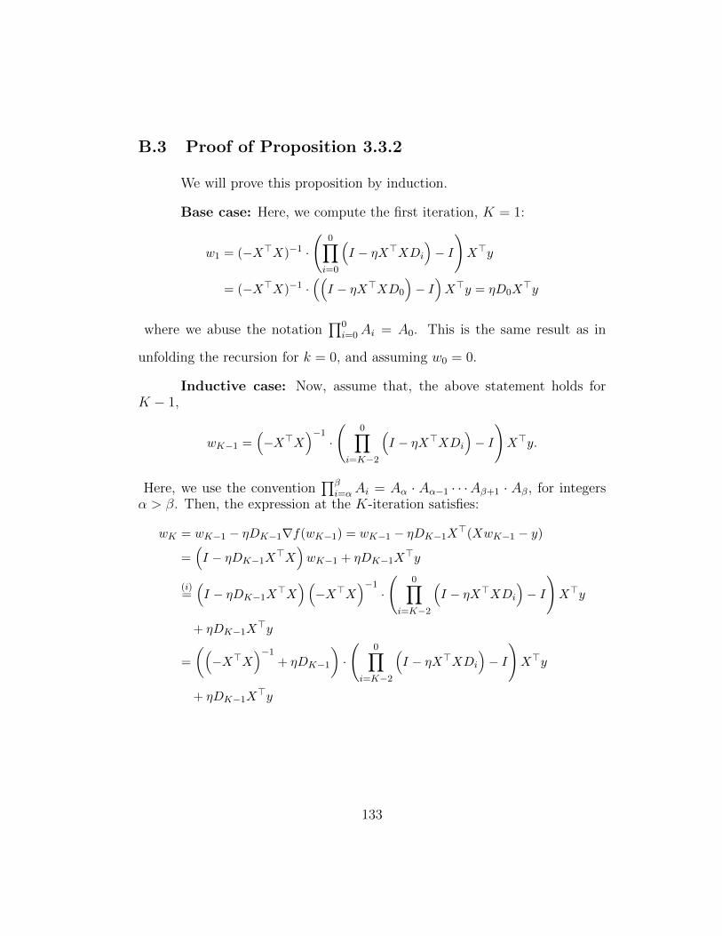
B.3 Proof of Proposition 3.3.2
We will prove this proposition by induction.
Base case: Here, we compute the first iteration, K = 1:
w1 = (−X>X)−1 ·(
0∏i=0
(I − ηX>XDi
)− I)X>y
= (−X>X)−1 ·((I − ηX>XD0
)− I)X>y = ηD0X
>y
where we abuse the notation∏0
i=0Ai = A0. This is the same result as in
unfolding the recursion for k = 0, and assuming w0 = 0.
Inductive case: Now, assume that, the above statement holds forK − 1,
wK−1 =(−X>X
)−1·(
0∏i=K−2
(I − ηX>XDi
)− I)X>y.
Here, we use the convention∏β
i=αAi = Aα · Aα−1 · · ·Aβ+1 · Aβ, for integersα > β. Then, the expression at the K-iteration satisfies:
wK = wK−1 − ηDK−1∇f(wK−1) = wK−1 − ηDK−1X>(XwK−1 − y)
=(I − ηDK−1X
>X)wK−1 + ηDK−1X
>y
(i)=(I − ηDK−1X
>X)(−X>X
)−1·(
0∏i=K−2
(I − ηX>XDi
)− I)X>y
+ ηDK−1X>y
=
((−X>X
)−1+ ηDK−1
)·(
0∏i=K−2
(I − ηX>XDi
)− I)X>y
+ ηDK−1X>y
133

=
((−X>X
)−1+ ηDK−1
)( 0∏i=K−2
(I − ηX>XDi
))X>y
−((−X>X
)−1+ ηDK−1
)X>y + ηDK−1X
>y
=
((−X>X
)−1+ ηDK−1
)( 0∏i=K−2
(I − ηX>XDi
))X>y −
(−X>X
)−1X>y
=(−X>X
)−1 (I − ηX>XDK−1
)( 0∏i=K−2
(I − ηX>XDi
))X>y
−(−X>X
)−1X>y
=(−X>X
)−1(
0∏i=K−1
(I − ηX>XDi
))X>y −
(−X>X
)−1X>y
=(−X>X
)−1(
0∏i=K−1
(I − ηX>XDi
)− I)X>y
where (i)(i)(i) is due to the inductive assumption. This completes the proof.
B.4 Proof of Proposition 3.4.1
Proposition B.4.1. The set of eigenvalues for D(t) is identical to the set of
eigenvalues of D(t).
Proof. We know for each t ≥ 0 that D(t) = V TD(t)V . As the matrix D(t) is
full rank for any t ≥ 0 we can write its SVD as D(t) = V D(t)ΛD(t)VTD(t). Sub-
stituting the SVD form in the expression we obtain D(t) = V TV D(t)ΛD(t)VTD(t)V .
But as both V D(t) and V forms basis of Rd we have V D(t)V as another ba-
sis. Therefore, V TD(t)V is the matrix of eigenvectors and ΛD(t) the eigenvalue
matrix for D(t). This proves our claim.
134

B.5 Proof of Proposition 3.4.2
The adaptive updates in (3.5) can be expressed in the spectral bases as
(w(t+ 1)− w(t))− ηλD(t)w(t)
= −ηV TV D(t)V TXT (XV (w(t)− w∗) +Uζ)
= −ηD(t)V TV ΛUT (UΛV TV (w(t)− w∗) +Uζ)
= −ηD(t)(Λ2(w(t)− w∗) + Λζ)
Therefore, the update in the spectral domain is represented as
w(t+ 1) =(I − ηD(t)(Λ2 + λI)
)w(t) + ηD(t)(Λ2w∗ + Λζ)
Using induction the closed form of the update in spectral domain can
be obtained as
w(T ) =T−1∏i=0
(I − ηD(i)(Λ2 + λI)
)w(0)
+T−1∑i=0
T−1∏j=(i+1)
(I − ηD(j)(Λ2 + λI)
)ηD(i)(Λ2w∗ + Λζ) (B.1)
The base case is true trivially. Given the expression is true for all the iterationsupto (T − 1) we have
w(T ) =(I − ηD(T − 1)(Λ2 + λI)
)w(T − 1) + ηD(T − 1)(Λ2w∗ + Λζ)
=(I − ηD(T − 1)(Λ2 + λI)
) T−1∏i=0
(I − ηD(i)(Λ2 + λI)
)w(0)
+
T−2∑i=0
(I − ηD(T − 1)(Λ2 + λI)
) T−2∏j=(i+1)
(I − ηD(j)(Λ2 + λI)
)ηD(i)(Λ2w∗ + Λζ)
+ ηD(T − 1)(Λ2w∗ + Λζ).
This completes the proof.
135

B.6 Proof of Proposition 3.4.3
From Theorem 3.2.1, we know that a sufficient condition for the con-
vergence under update (3.5) is
supt≥1|λ(I − ηD(t)(Λ2 + λI)
)| < 1.
Thus, for λ > 0, the dynamics converges to a bounded weight vector for any
η ∈(
0, 2 (λmax(D(t))(λ2max(X) + λ))
−1).
We now characterize the fixed point of the dynamics in (3.5). When
the convergence happens, for any fixed point w of the updates in (3.5)
D(t)(λw +XTX(w −w∗)−XTw
)= 0.
Because, inft rank(D(t)) = d (full rank) we must have
λw +XTX(w −w∗)−XTw = 0
. Expanding the L.H.S. in terms of the SVD of the data matrix we obtain,
d∑r=1
λwrvr +R∑r=1
(λ2rwr − λ2
rw∗r − λrζr
)vr = 0.
Therefore, for λ ≥ 0 (holds for both regularized and unregularized) we have
vrT w = λ2rw
∗r+λr ζrλ+λ2r
for r ≤ R. Further, for λ > 0, vrT w = 0 for r ≥ (R + 1).
B.7 Proof of Lemma B.7.1
Using the above structure we obtain the following lemma concerning the
closed form expression of the iterates. Let us define for any matrix A ∈ Rd×d
136

and any vector b ∈ Rd:
A(1) = Aij : 1 ≤ i, j ≤ R,
A(2) = Aij : R + 1 ≤ i ≤ d, 1 ≤ j ≤ R,
b(1) = bi : 1 ≤ i ≤ R,
b(2) = bi : R + 1 ≤ i ≤ d,
where R is the rank of the data matrix D and d is the dimension of the data.
Lemma B.7.1. If D(t) is full rank for all t ≥ 0 and regularizer λ = 0,
then for any T ≥ 0, the closed form of the iterate w(T ) admits the following
expression:
w(1)(T ) = A(T−1, 0)w1(0)
+T−1∑i=0
A(T−1, i+1)ηD(1)(i)Λ2(1)(w
∗(1) + Λ−1
(1)ζ(1)),
w(2)(T ) = B(T−1, 0)w(1)(0) + w(2)(0)
+T−1∑i=0
η(B(T−1, i+1)D(1)(i)+D(2)(i)
)×
×Λ2(1)(w
∗(1) + Λ−1
(1)ζ(1)),
where for all t2 ≥ t1 ≥ 0,
A(t2, t1) =
t2∏i=t1
(I − ηD(1)(i)Λ
2(1)
)B(t2, t1)=− ηD(2)(t1)Λ2
(1)
−ηt2∑
i=t1+1
D(2)(i)Λ2(1)A(i−1, t1)
137
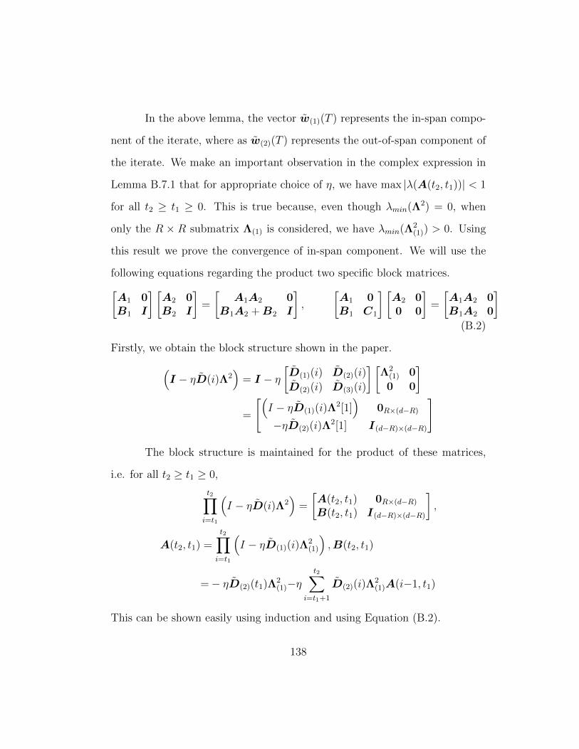
In the above lemma, the vector w(1)(T ) represents the in-span compo-
nent of the iterate, where as w(2)(T ) represents the out-of-span component of
the iterate. We make an important observation in the complex expression in
Lemma B.7.1 that for appropriate choice of η, we have max |λ(A(t2, t1))| < 1
for all t2 ≥ t1 ≥ 0. This is true because, even though λmin(Λ2) = 0, when
only the R × R submatrix Λ(1) is considered, we have λmin(Λ2(1)) > 0. Using
this result we prove the convergence of in-span component. We will use the
following equations regarding the product two specific block matrices.[A1 0B1 I
] [A2 0B2 I
]=
[A1A2 0
B1A2 +B2 I
],
[A1 0B1 C1
] [A2 00 0
]=
[A1A2 0B1A2 0
](B.2)
Firstly, we obtain the block structure shown in the paper.(I − ηD(i)Λ2
)= I − η
[D(1)(i) D(2)(i)
D(2)(i) D(3)(i)
] [Λ2
(1) 0
0 0
]=
[(I − ηD(1)(i)Λ
2[1])
0R×(d−R)
−ηD(2)(i)Λ2[1] I(d−R)×(d−R)
]
The block structure is maintained for the product of these matrices,
i.e. for all t2 ≥ t1 ≥ 0,
t2∏i=t1
(I − ηD(i)Λ2
)=
[A(t2, t1) 0R×(d−R)
B(t2, t1) I(d−R)×(d−R)
],
A(t2, t1) =
t2∏i=t1
(I − ηD(1)(i)Λ
2(1)
),B(t2, t1)
=− ηD(2)(t1)Λ2(1)−η
t2∑i=t1+1
D(2)(i)Λ2(1)A(i−1, t1)
This can be shown easily using induction and using Equation (B.2).
138

Substituting these results in the closed form of the iterates in proposi-
tion 3.4.2 we obtain
w(T ) =
[A(T−1, 0)w1(0)
B(T−1, 0)w1(0) + w(2)(0)
]+
T−1∑i=0
[A(T−1, i+1) 0B(T−1, i+1) I
] [ηD1(i)Λ2
1(w∗1 + Λ−11 ζ1)
ηD(2)(i)Λ21(w∗1 + Λ−1
1 ζ1)
]
In-span Component: Therefore, the component of in the span of data is
w(T )
w(1)(T ) = A(T−1, 0)w1(0) +T−1∑i=0
A(T−1, i+1)ηD1(i)Λ2(1)(w
∗(1) + Λ−1
(1)ζ(1)),
Similar to the regularized case, we have for any
η ∈(
0, 2(λmax(D(t))(λ2
max(X)))−1)
the in-span component converges. Further, from the fixed point argument we
know that vTr w = w∗r + λ−1r ζr.
Out-of-span Component: The component outside the span of the data is
w(2)(T ) = B(T−1, 0)w(1)(0) + w(2)(0)
+T−1∑i=0
η(B(T−1, i+1)D(1)(i)+D(2)(i)
)Λ2
(1)(w∗(1) + Λ−1
(1)ζ(1)).
139

B.8 Proof of Theorem 3.4.5
The convergence of the in-span component follows similar to the regu-
larized case. In particular, we observe
λmax(I − ηD(1)(t)Λ2(1)) ≤ 1− ηλmin(D(1)(t))λmin(Λ2
(1)) < 1.
The last inequality is true as 1) λmin(D(1)(t)) > 0 due to the positive definite-
ness of the matrix D(t), and 2) λmin(Λ2(1)) > 0 as it considers only the in-span
component (i.e. the top-left R × R sub-matrix of Λ). On the other hand, we
have λmin(I−ηD(1)(t)Λ2(1)) ≥ 1−ηλmax(D(1)(t))λmax(Λ
2(1)). Therefore, we ob-
tain λmin(I−ηD(1)(t)Λ2(1)) > −1 for any 0 < η < 2/(λmax(D(1)(t))λmax(Λ
2(1))).
As D(1)(t) is a principal sub-matrix of D(t) for each t ≥ 0, we have
from Cauchy Interlacing Theorem λmax(D(1)(t)) ≤ λmax(D(t)) = λmax(D(t)).
The last equality is due to Proposition 3.4.1. The characterization of the fixed
point follows the same argument as Proposition 3.4.3.
To prove the second part, we further simplify the out-of-span compo-
nent using exchange of summation (for finite T ). Here, we use the convention
140

A(t1, t2) = I for any t1 < t2.
w(2)(T )−(B(T−1, 0)w(1)(0) + w(2)(0)
)=
T−1∑i=0
η(D(2)(i)− ηD(2)(i+ 1)Λ2
(1)D(1)(i)−
ηT−1∑j=i+2
D(2)(i)Λ2(1)A(j−1, i+ 1)D(1)(i)
)Λ2
(1)(w∗(1) + Λ−1
(1)ζ(1)).
=
(T−1∑i=0
ηD(2)(i)− η2
T−1∑i=0
T−1∑j=i+1
D(2)(j)Λ2(1)A(j−1, i+ 1)D(1)(i)
)Λ2
(1)(w∗(1) + Λ−1
(1)ζ(1)).
=
(T−1∑i=0
ηD(2)(i)
(I − ηΛ2
(1)
i−1∑j=0
A(i−1, j + 1)D(1)(j)
))Λ2
(1)(w∗(1) + Λ−1
(1)ζ(1)),
=
(T−1∑i=0
ηD(2)(i)(Λ2
(1)(w∗(1) + Λ−1
(1)ζ(1))−Λ2(1)w(1)(i) + Λ2
(1)A(i−1, 0)w1(0)))
,
=T−1∑i=0
ηD(2)(i)Λ2(1)
((w∗(1) + Λ−1
(1)ζ(1))− w(1)(i))
+T−1∑i=0
ηD(2)(i)Λ2(1)A(i−1, 0)w1(0).
Therefore, we have
‖w(2)(T )− w(2)(0)‖2
≤T−1∑i=0
ηD(2)(i)Λ2(1)
((w∗(1) + Λ−1
(1)ζ(1))− w(1)(i))
+
(B(T−1, 0) +
T−1∑i=0
ηD(2)(i)Λ2(1)A(i−1, 0)
)w1(0)
=T−1∑i=0
ηD(2)(i)Λ2(1)
((w∗(1) + Λ−1
(1)ζ(1))− w(1)(i))− ηD(2)(0)Λ2
(1)w1(0)
We have |λ|max = supt |λmax(I − η ˜D1(t)Λ2(1))| < 1 due to appropriate
choice of η. Also, by assumption of the theorem we have for some α ≥ 0,
141

β ≥ 0, α + β > 1, for some universal constants 0 < cconv, cλ < ∞, and for all
t ≥ 0:
(i) the out-of-span pre-conditioner matrix decaying as O(1/tα) for some
α ≥ 0, i.e. |λmax(D(2)(i))| = cλ(t+1)α
, and
(ii) the convergence rate of the in-span component is O(1/tβ) with
iteration t for some β > 0, i.e. ‖(w∗(1) + Λ−1(1)ζ(1))− w(1)(i)‖2 ≤ cconv
(t+1)β.
For the first term we have,
‖T−1∑i=0
ηD(2)(i)Λ2(1)
((w∗(1) + Λ−1
(1)ζ(1))− w(1)(i))‖2
≤ cλ
T−1∑i=0
λmax(D(2)(i))‖(w∗(1) + Λ−1(1)ζ(1))− w(1)(i)‖2
≤ cλcconv
T−1∑i=1
1(i+1)(α+β)
≤ cλcconvα+β−1
(1− 1
(i+1)(α+β−1)
).
Therefore, the first term saturates to a value at most cλcconvα+β−1
.
For the second term we have,
‖ηD(2)(0)Λ2(1)w1(0)‖2 ≤ ηλmax(D(2)(0))λ2
max(Λ(1))‖w1(0)‖2
B.9 Proof of Proposition B.9.1
Proposition B.9.1. The following pre-conditioner matrices have D(2)(t) = 0.
1. D(t) = I, i.e. gradient descent,
2. D(t) = (XTX + εI)−1 for all t ≥ 0.
142

We have (XTX + εI)−1 =∑R
r=1(λ2r + ε)−1vrv
Tr +
∑dr=R+1 ε
−1vrvTr .
Further, I =∑d
r=1 bsvrvTr . So the proposition is true.
B.10 Proof of Lemma 3.5.1
Proposition B.10.1. Suppose X>y has no zero components. Define D =
diag(|X>y|3) and assume there exists a scalar c such thatXD−1sign(X>y) =
cy. Then, when initialized at 0, the AdaGrad variant in (3.9) converges to the
unique solution w ∝D−1sign(X>y).
We will prove this using induction. Let Q = diag(|XTy|) We will show
that
wk = λkQ−1sign(XTy)
for some λk. w0 = 0 is satsified for λ0 = 0 and so the base case is trivially
true.
gk = XT (Xwk − y)
= λkXTXQ−1sign(XTy)−XTy
= (λkc− 1)XTy
where the last inequality follows from wk = λkQ−1sign(XTy).3
Hk = diag(n∑s=1
gs · gs) = νkdiag(|XTy|2) = νkQ2
143

wk+1 = wk − αkH−1k XT (Xwk − y)
= wk − αkH−1k XTXwk + αkH
−1k XTy
= λkQ−1sign(XTy)− λkαkH−1
k XTXQ−1XTy + αkH−1k XTy
= λkQ−1sign(XTy)− λkαkcH−1
k XTy + αkH−1k XTy
=
(λk −
λkαkc
νk+αkνk
)Q−1sign(XTy)
= λk+1Q−1sign(XTy)
B.11 More details and experiments for the counter-example
The simulation is completed as follows: For each setting (n, p, J), we
generate 100 different instances for (X, y), and for each instance we compute
the solutions from gradient descent, AdaGrad variant and Adam (RMSprop
is included in the Appendix) and the minimum norm solution wmn. In the
appendix, we have the above table with the Adagrad variant that normalizes
the final solution w (Table ??) before calculating the distance w.r.t. the mini-
mum norm solution: we observed that this step did not improve or worsen the
performance, compared to the unnormalized solution. This further indicates
that there is an infinite collection of solutions –with different magnitudes– that
lead to better performance than plain gradient descent; thus our findings are
not a pathological example where adaptive methods work better.
We record ‖w−wmn‖2, where w represents the corresponding solutions
obtained by the algorithms in the comparison list. For each (X, y) instance,
144
we further generate ytesti , xtest
i 100i=1, and we evaluate the performance of both
models on predicting ytesti , ∀i.
Table 3.4 shows that gradient descent converges to the minimum norm
solution, in contrast to the adaptive methods. This justifies the fact that the
adaptive gradient methods (including the proposed adagrad variant) converge
to a different solution than the minimum norm solution. Nevertheless, the ac-
curacy on unseen data is higher in the adaptive methods (both our proposed
AdaGrad variant and in most instances, Adam), than the plain gradient de-
scent, when ` is small: the adaptive method successfully identifies the correct
class, while gradient descent only predicts one class (the positive class; this
is justified by the fact that the accuracy obtained is approximately close to
p, as n increases). We first provide the same table in Table 3.4 but with
unnormalized values for distances with respect to Adagrad variant.
Here, we provide further results on the counterexample in Subsubsec-
tion 3.5.1.1. Tables ?? and B.1 contains results for J = 10: the purpose of
these tables is to show that even if we change the memory use footprint of
the AdaGrad variant—by storing fewer or more gradients to compute Dk in
(3.9)—the results are the same: the AdaGrad variant consistently converges
to a solution different than the minimum norm solution, while being more
accurate than the latter for small values of ` (i.e., smaller margin between the
two classes).
Plain gradient descent methods provably need to rely on the first ele-
145

GD ADAVAR ADAM
n = 10
` = 1/32Acc. (%) 63 100 91‖w − wmn‖2 1.015 · 10−16 0.9911 0.1007
` = 1/16Acc. (%) 53 100 87‖w − wmn‖2 1.7401 · 10−16 0.9263 0.0864
` = 1/8Acc. (%) 58 99 84‖w − wmn‖2 4.08 · 10−16 0.8179 0.0764
n = 50
` = 1/32Acc. (%) 77 100 88‖w − wmn‖2 4.729 · 10−15 0.8893 0.0271
` = 1/16Acc. (%) 80 100 89‖w − wmn‖2 6.9197 · 10−15 0.7929 0.06281
` = 1/8Acc. (%) 91 100 89‖w − wmn‖2 9.7170 · 10−15 0.6639 0.1767
n = 100
` = 1/32Acc. (%) 85 100 95‖w − wmn‖2 4.975 · 10−9 0.8463 0.0344
` = 1/16Acc. (%) 83 100 76‖w − wmn‖2 2.5420 · 10−9 0.7217 0.1020
` = 1/8Acc. (%) 100 100 90‖w − wmn‖2 1.5572 · 10−11 0.6289 0.3306
Table B.1: Prediction accuracy and distances from the minimum norm solution forplain gradient descent and adaptive gradient descent methods. We set p = 7/8 andJ = 10, as in the main text. The adaptive method uses Dk according to (3.9). Thedistances shown are median values out of 100 different realizations for each setting;the accuracies are obtained by testing 104 predictions on unseen data.
146

ments to decide; using the same rule for adaptive methods1. The remaining
subsection considers the case where we decide based on the y = sign(x>w)
rule, where w is the complete learned model. As we show empirically, more
often than not adaptive methods outperform plain gradient methods.
Observing the performance of various optimization techniques for dif-
ferent values of n, p and `, we observed that the best performances are obtained
when the dataset is highly imbalanced irrespective of the optimization algo-
rithm chosen. When the data is (almost) balanced, it is difficult to comment
on how the performance of these algorithms is affected by variations in the
levels ` and probability p.
B.12 Deep Learning
In this section, we will extend the experiments to over-parameterized
and under-parameterized neural networks without regularization. We begin
with a detailed description of the datasets and the architectures we use along
with comprehensive set of experiments with hyperparameter tuning.
MNIST dataset and the M1 architecture. Each experiment for M1 is
simulated over 50 epochs and 10 runs for both under- and over-parameterized
settings. Both the MNIST architectures consisted of two convolutional layers
1We note that using only the three elements in adaptive methods is not backed up bytheory since it assumes that the training and test datasets have no overlap. We include thisin comparison for completeness.
147

Name Network type Dataset
M1-UP Shallow CNN + FFN MNISTM1-OP Shallow CNN + FFN MNISTC1-UP Shallow CNN + FFN CIFAR-10C1-OP ResNet18 CIFAR-10C2-OP PreActResNet18 CIFAR-100C3-OP MobileNet CIFAR-100C4-OP MobileNetV2 CIFAR-100C5-OP GoogleNet CIFAR-100
Table B.2: Summary of the datasets and the architectures used for experiments.CNN stands for convolutional neural network, FF stands for feed forward network.More details are given in the main text.
(the second one with dropouts [79]) followed by two fully connected layers. The
primary difference between the M1-OP (∼ 73K parameters) and M1-UP (∼
21K parameters) architectures was the number of channels in the convolutional
networks and # of nodes in the last fully connected hidden layer.
Figure 3.3, left two columns, reports the results over 10 Monte-Carlo
realizations. Top row corresponds to the M1-UP case; bottom row to the M1-
OP case. We plot both training errors and the accuracy results on unseen
data. For the M1-UP case, despite the grid search, observe that AdaGrad
(and its variant) do not perform as well as the rest of the algorithms. Never-
theless, adaptive methods (such as Adam and RMSProp) perform similarly to
simple SGD variants, supporting our conjecture that each algorithm requires
a different configuration, but still can converge to a good local point; also
that adaptive methods require the same (if not more) tuning. For the M1-OP
case, SGD momentum performs less favorably compared to plain SGD, and
148
we conjecture that this is due to non-optimal tuning. In this case, all adaptive
methods perform similarly to SGD.
CIFAR10 dataset and the C1 architecture. For C1, C1-UP is trained
over 350 epochs, while C1-OP was trained over 200 epochs. The under-
parameterized setting is on-purpose tweaked to ensure that we have fewer pa-
rameters than examples (∼ 43K parameters), and slightly deviates from [158];
our generalization guarantees (∼ 76%) are in conjunction with the attained
test accuracy levels. Similarly, for the C1-OP case, we implement a Resnet
[80] + dropout architecture (∼ 0.25 million parameters) Adam and RMSProp
achieves the best performance than their non-adaptive counterparts for both
the under-parameterized and over-parameterized settings.
Figure 3.3, right panel, follows the same pattern with the MNIST data;
it reports the results over 10 Monte-Carlo realizations. Again, we observe
that AdaGrad methods do not perform as well as the rest of the algorithms.
Nevertheless, adaptive methods (such as Adam and RMSProp) perform simi-
larly to simple SGD variants. Further experiments on CIFAR-100 for different
architecture are provided in the Appendix.
CIFAR100 and other deep architectures (C2-5-OP). In this ex-
periment, we focus only on the over-parameterized case: DNNs are usually
designed over-parameterized in practice, with ever growing number of layers,
and, eventually, a larger number of parameters [81]. We again completed
149

10 runs for each of the set up we considered. C2-OP corresponds to Pre-
ActResNet18 from [5], C3-OP corresponds to MobileNet from [6], C4-OP is
MobileNetV2 from [7], and C5-OP is GoogleNet from [82]. The results are
depicted in Figure 3.4. After a similar hyper-parameter tuning phase, we se-
lected the best choices among the parameters tested. The results show no
clear winner once again, which overall support our claims: the superiority de-
pends on the problem/data at hand; also, all algorithms require fine tuning to
achieve their best performance. We note that a more comprehensive reasoning
requires multiple runs for each network, as other hyper-parameters (such as
initialization) might play significant role in closing the gap between different
algorithms.
An important observation of Figure 3.4 comes from the bottom row
of the panel. There, we plot the Euclidean norm ‖ · ‖2 of all the trainable
parameters of the corresponding neural network. While such a norm could be
considered arbitrary (e.g., someone could argue other types of norms to make
more sense, like the spectral norm of layer), we use the Euclidean norm as i)i)i)
it follows the narrative of algorithms in linear regression, where plain gradient
descent algorithms choose minimum `2-norm solutions, and ii)ii)ii) there is recent
work that purposely regularizes training algorithms towards minimum norm
solutions [83].
Our findings support our claims: in particular, for the case of MobileNet
and MobileNetV2, Adam, an adaptive method, converges to a solution that
has at least as good generalization as plain gradient methods, while having 2×
150

larger `2-norm weights. However, this may not always be the trend: in Figure
3.4, left panel, the plain gradient descent models for the PreActResNet18
architecture [5] show slightly better performance, while preserving low weight
norm. The same holds also for the case of GoogleNet; see Figure 3.4, right
panel.
B.12.0.1 Hyperparameter tuning
Both for adaptive and non-adaptive methods, the step size and mo-
mentum parameters are key for favorable performance, as also concluded in
[71]. Default values were used for the remaining parameters. The step size was
tuned over an exponentially-spaced set 0.0001, 0.001, 0.01, 0.1, 1, while the
momentum parameter was tuned over the values of 0, 0.1, 0.25, 0.5, 0.75, 0.9.
We observed that step sizes and momentum values smaller/bigger than these
sets gave worse results. Yet, we note that a better step size could be found be-
tween the values of the exponentially-spaced set. The decay models were similar
to the ones used in [71]: no decay and fixed decay. We used fixed decay in the
over-parameterized cases, using the StepLR implementation in pytorch. We
experimented with both the decay rate and the decay step in order to ensure
fair comparisons with results in [71].
B.12.0.2 Results
Our main observation is that, both in under- or over-parameterized
cases, adaptive and non-adaptive methods converge to solutions with similar
151

testing accuracy: the superiority of simple or adaptive methods depends on the
problem/data at hand. Further, as already pointed in [71], adaptive methods
often require similar parameter tuning. Most of the experiments involve using
readily available code from GitHub repositories. Since increasing/decreasing
batch-size affects the convergence [84], all the experiments were simulated on
identical batch-sizes. Finally, our goal is to show performance results in the
purest algorithmic setups: often, our tests did not achieve state of the art
performance.
Overall, despite not necessarily converging to the same solution as gra-
dient descent, adaptive methods generalize as well as their non-adaptive coun-
terparts. In M1 and C1-UP settings, we compute standard deviations from
all Monte Carlo instances, and plot them with the learning curves (shown
in shaded colors is the one-apart standard deviation plots; best illustrated in
electronic form). For the cases of C1-5-OP, we also show the weight norms
of the solutions (as in Euclidean distance ‖ · ‖2 of all the trainable weights in
the network). Such measure has been in used in practice [83], as a regulariza-
tion to find minimum Euclidean norm solutions, inspired by the results from
support vector machines [45].
We observe that adaptive methods (such as Adam and RMSProp) per-
form similarly to simple SGD variants, supporting our conjecture that each
algorithm requires a different configuration, but still can converge to a good
local point; also that adaptive methods require the same (if not more) tun-
ing. Again, we observe that AdaGrad methods do not perform as well as the
152

rest of the algorithms. Nevertheless, adaptive methods (such as Adam and
RMSProp) perform similarly to simple SGD variants. Further experiments on
CIFAR-100 for different architecture are provided in the Appendix.
153

Appendix C
Appendix
C.1 Additional Results for Section 3
The following lemma provides upper bounds on the expected gradient
of the worst-possible MKL-SGD solution that lies in a ball around w∗. Simul-
taneously satisfying the following bound with the one in Lemma 4.3.4 may lead
to an infeasible set of ε and N ′. And thus we use Lemma 4.3.5 in conjunction
with 4.3.4.
Lemma C.1.1. Let us assume that MKL-SGD converges to wMKL. For any
wMKL ∈ Br(w∗) that satisfies assumptions N1, N2, A4 and A5, there exists
N ′ ≥ N and ε′ ≤ ε such that,
‖∑i/∈O
pi(wMKL)∇fi(wMKL)‖
≤ min
(1− εk)L‖wMKL −w∗‖, εkG(w)
The proof for lemma 2 can be found in the Appendix Section C.2.7
154

C.2 Proofs and supporting lemmas
C.2.1 Proof of Lemma 4.3.1
Proof. F (w) =∑
i pmi(w)(w). Let us fix a w such that pi = pi(w). We know
that for any pi,∑
i pifi(w) is strongly convex in w with parameter λw. This
implies
∇F (w)>(w −w∗) ≥ λ‖w −w∗‖2
C.2.2 Proof of Theorem 4.3.2
Proof. By the definition of the noiseless framework, w∗ is the unique optimum
of F (w) and lies in the optimal set of each fi(.). We will prove this theorem by
contradiction. Assume there exists some w 6= w∗ that also satisfies optimum
of ∇F (w) = 0. At w, we have 0 =< ∇F (w), w −w∗ >= λ‖w −w∗‖2. This
implies w = w∗.
C.2.3 Proof of Lemma 4.3.3
Let w be a stationary point of MKL-SGD . Now, we analyze the loss
landscape on the line joining w∗ and wC where wC = Cw is any arbitrary
point 1 in the landscape at a distance as far as the farthest outlier from w∗.
Let C be a very large number.
1Note that we just needwC for the purpose of landscape analysis and it is not a parameterof the algorithm
155

The loss functions and w are redefined as follows:
fi(w) =
li‖w −w∗‖2 ∀ i ∈ Oli‖w −wbi‖2 ∀ i /∈ O,
w :=
w∣∣∣∣ w = min
α∈(0,1)αw∗ + (1− α)wC ,
flm(w) = flM (w)
where |O| = b such that n = g + b. Let lm = mini/∈O li and Let
lM = maxi∈O li and lmax = mini∈[n] li, lmin = mini∈[n] li. Let us define κ =
lmaxlmin
≥ lMlm
.
Now at w, we have ∇F (w) = 0. Let us assume that the outliers are
chosen in such a way that atwC , all the outliers have the lowest loss. As stated
in the previous lemma, the results hold irrespective of that. This implies:
∑i/∈O
pi(wC)∇fi(w) = −∑j∈O
pj(wC)∇fj(w)∑i/∈O
pi(wC)li(w −w∗) = −∑j∈O
pj(wC)lj(w −wbj)
w =
∑i/∈O pi(wC)liw
∗ +∑
j∈O pj(wC)ljwbj∑i/∈O pi(wC)li +
∑j∈O pj(wC)lj
By triangle inequality, ‖w −w∗‖ ≤∑
j∈O pj(wC)lj‖wbj −w∗‖∑i/∈O pi(wC)li +
∑j∈O pj(wC)lj
Without loss of generality assume that the outliers are ordered as fol-
lows: ‖wb1 −w∗‖ ≤ ‖wb2 −w∗‖ ≤ · · · ≤ ‖wb|O| −w∗‖.
Now w be some point of intersection of function in the set of clean
samples and a function in the set of outliers tow∗. Let θj be the angle between
156
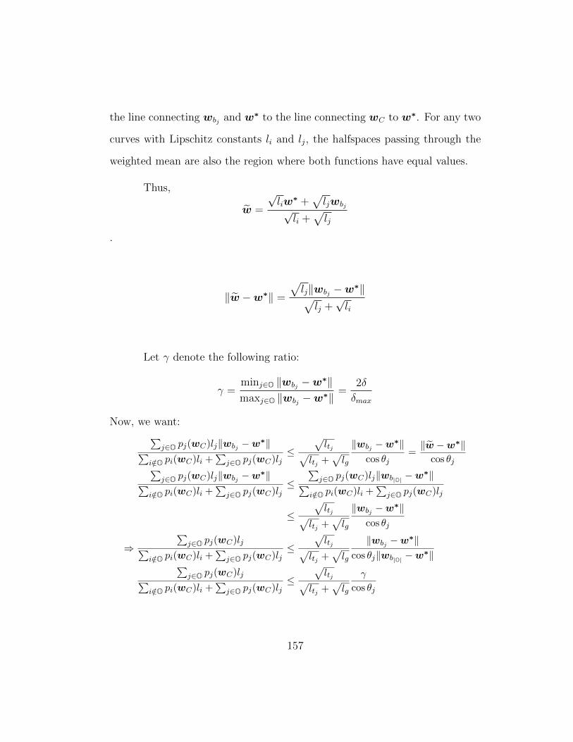
the line connecting wbj and w∗ to the line connecting wC to w∗. For any two
curves with Lipschitz constants li and lj, the halfspaces passing through the
weighted mean are also the region where both functions have equal values.
Thus,
w =
√liw∗ +
√ljwbj√
li +√lj
.
‖w −w∗‖ =
√lj‖wbj −w∗‖√lj +√li
Let γ denote the following ratio:
γ =minj∈O ‖wbj −w∗‖maxj∈O ‖wbj −w∗‖
=2δ
δmax
Now, we want:∑j∈O pj(wC)lj‖wbj −w∗‖∑
i/∈O pi(wC)li +∑
j∈O pj(wC)lj≤
√ltj√
ltj +√lg
‖wbj −w∗‖cos θj
=‖w −w∗‖
cos θj∑j∈O pj(wC)lj‖wbj −w∗‖∑
i/∈O pi(wC)li +∑
j∈O pj(wC)lj≤
∑j∈O pj(wC)lj‖wb|O| −w∗‖∑
i/∈O pi(wC)li +∑
j∈O pj(wC)lj
≤√ltj√
ltj +√lg
‖wbj −w∗‖cos θj
⇒∑
j∈O pj(wC)lj∑i/∈O pi(wC)li +
∑j∈O pj(wC)lj
≤√ltj√
ltj +√lg
‖wbj −w∗‖cos θj‖wb|O| −w∗‖∑
j∈O pj(wC)lj∑i/∈O pi(wC)li +
∑j∈O pj(wC)lj
≤√ltj√
ltj +√lg
γ
cos θj
157

For simplicity, Γ =γ
cos θj, then we have:
∑j∈O pj(wC)lj∑
i/∈O pi(wC)li +∑
j∈O pj(wC)lj≤
√ltj√
ltj +√lg
Γ
1
Γ
(√lg√ltj
+ 1
)− 1 ≤ (1− p)lm
plM≤∑
i/∈O pi(wC)li∑j∈O pj(wC)lj
p
1− p ≤lmlM
1Γ− 1 + 1
Γ
√lg√ltj
p ≤ 1
1 + κ(
1Γ− 1 +
√κ
Γ
)≤ 1
1 + lMlm
(1Γ− 1 + 1
Γ
√lg√ltj
)
Replacing Γ =γ
cos θj, and let q =
cos θjγ− 1 +
cos θj√κ
γthe condition to
guarantee that bad local minima do no exist is p ≤ 1
1 + κqand q > 0.
Note: In the vector case, for example there exists a fine tradeoff be-
tween how large θj can be and if for large θj, the loss corresponding to the
outlier will be one of the lowest. Understanding that tradeoff is beyond the
scope of this paper.
158

C.2.4 Proof of Lemma 4.3.4
Proof. At wSGD, ∇F (wSGD) = 0. Then,
∑i/∈O
∇fi(wSGD) = −∑i∈O
∇fi(wSGD)
‖∑i/∈O
∇fi(wSGD)‖ = ‖∑i∈O
∇fi(wSGD)‖
‖∑i/∈O
∇fi(wSGD)‖ ≤∑i
‖∇fi(wSGD)‖
≤∑i
L‖wSGD −w∗‖
= (1− ε)nL‖wSGD −w∗‖ (C.1)
‖∑i∈O
∇fi(wSGD)‖ ≤∑i∈O
‖∇fi(wSGD)‖
≤∑i∈O
G(wSGD)
≤ εG(wSGD) (C.2)
‖∑i∈O
∇fi(wSGD)‖ = min (εnG(wSGD), (1− ε)nL‖wSGD −w∗‖)
159

C.2.5 Proof of Lemma 4.3.5
Proof. At wMKL, ∇F (wMKL) = 0. This implies
∑i/∈O
pi(wMKL)∇fi(wMKL) = −∑i∈O
pi(wMKL)∇fi(wMKL)
Multiplying both sides by (wMKL −w∗)∑i/∈O
pi(wMKL) < ∇fi(wMKL), wMKL −w∗ >
= −∑i∈O
pi(wMKL) < ∇fi(wMKL), wMKL −w∗ >
< ∇FG(wMKL), wMKL −w∗ >
= −∑i∈O
pi(wMKL) < ∇fi(wMKL), wMKL −w∗ >
Lower bounding the LHS using Lemma 4.3.1 and m = m(wMKL)2 ,
m‖wMKL −w∗‖2 ≤ ‖ < ∇FG(wMKL), wMKL −w∗ > ‖ = LHS
RHS ≤ ‖ −∑i∈O
pi(wMKL) < ∇fi(wMKL), wMKL −w∗ > ‖
m‖wMKL −w∗‖2 ≤∑i∈O
pi(wMKL)‖ < ∇fi(wMKL), wMKL −w∗ > ‖
m‖wMKL −w∗‖2 ≤∑i∈O
pi(wMKL)‖∇fi(wMKL)‖‖wMKL −w∗‖
m‖wMKL −w∗‖2 ≤∑i∈O
pi(wMKL)‖wMKL −w∗‖G(wSGD)
m‖wMKL −w∗‖ ≤ εkG(wSGD)
160

C.2.6 Proof of Theorem 4.3.6
Proof. There exists an ε′ ≤ ε such that in Lemma 4.3.4, we have
(1− ε)L‖wSGD −w∗‖ ≥ εG(wSGD)
Combining above equation with Lemma 4.3.5, we get
(1− ε)L‖wSGD −w∗‖ ≥ εG(wSGD) ≥ ελ
ε2‖wMKL −w∗‖
⇒ ‖wMKL −w∗‖ ≤(1− ε)Lεk−1
λ‖wSGD −w∗‖
Picking a large enough k, we can guarantee that(1− ε)Lεk−1
λ< 1
C.2.7 Proof of Lemma C.1.1
Proof. From the definition of good samples in the noiseless setting, we know
that fi(w∗) = 0 ∀ i /∈ O. Similarly, for samples belonging to the outlier set,
fi(w∗) > 0 ∀ i ∈ O. There exists a ball around the optimum of radius r such
that fi(w) ≤ fj(w) ∀i /∈ O, j ∈ O,w ∈ Or(w∗). Assume that N ′ ≥ N and
ε′ ≤ ε, such that ‖wMKL −w∗‖ ≤ r.
161
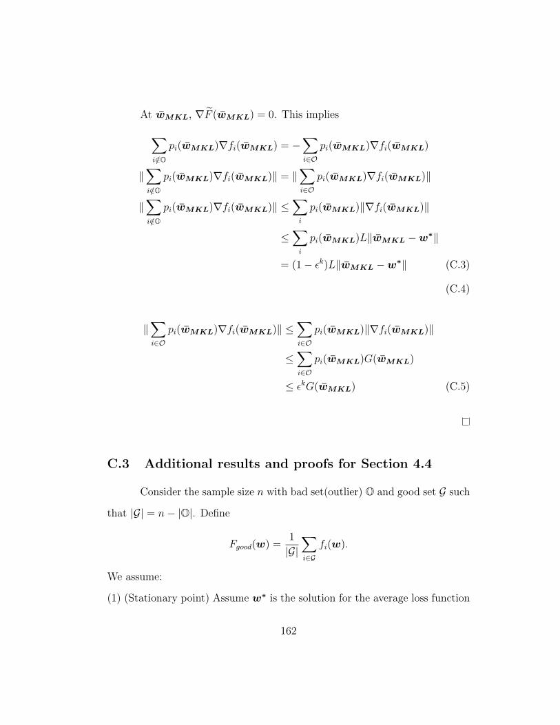
At wMKL, ∇F (wMKL) = 0. This implies
∑i/∈O
pi(wMKL)∇fi(wMKL) = −∑i∈O
pi(wMKL)∇fi(wMKL)
‖∑i/∈O
pi(wMKL)∇fi(wMKL)‖ = ‖∑i∈O
pi(wMKL)∇fi(wMKL)‖
‖∑i/∈O
pi(wMKL)∇fi(wMKL)‖ ≤∑i
pi(wMKL)‖∇fi(wMKL)‖
≤∑i
pi(wMKL)L‖wMKL −w∗‖
= (1− εk)L‖wMKL −w∗‖ (C.3)
(C.4)
‖∑i∈O
pi(wMKL)∇fi(wMKL)‖ ≤∑i∈O
pi(wMKL)‖∇fi(wMKL)‖
≤∑i∈O
pi(wMKL)G(wMKL)
≤ εkG(wMKL) (C.5)
C.3 Additional results and proofs for Section 4.4
Consider the sample size n with bad set(outlier) O and good set G such
that |G| = n− |O|. Define
Fgood(w) =1
|G|∑i∈G
fi(w).
We assume:
(1) (Stationary point) Assume w∗ is the solution for the average loss function
162

of good sample such that
∇Fgood(w∗) = 0 but ∇fi(w∗) 6= 0,∀i
(2) (Strong Convexity) Fgood(w) is strongly convex with parameters λgood i.e.,
〈∇Fgood(w)−∇Fgood(w∗),w −w∗〉 ≥ λgood‖w −w∗‖2
(3) (Gradient Lipschitz) fi(w) has Li Liptchitz gradient i.e.,
‖∇fi(w)−∇fi(w∗)‖ ≤ Li‖w −w∗‖
Theorem C.3.1. (Distance to w∗)
Ei[‖wt+1 −w∗‖2|wt
]≤(
1− 2ηtλgood(1− ηt supiLi)|G|n
)‖wt −w∗‖2 +Rt
(C.6)
where
Rt =− 2ηt(1− ηt supiLi))
∑i∈G
(pi(wt)−
1
n
)〈wt −w∗,∇fi(wt)−∇fi(w∗)〉
− 2ηt∑i∈G
pi(wt)〈wt −w∗,∇fi(w∗)〉+ 2η2t
∑i∈G
pi(wt)‖∇fi(w∗)‖2
+ η2t
∑i∈O
pi(wt)‖∇fi(wt)‖2 + 2ηt∑i∈O
pi(wt) (fi(w∗)− fi(wt))
Proof. Observe first that for each component function i.e. ,
〈w − v,∇fi(w)−∇fi(v)〉 ≥ 1
Li‖fi(w)− fi(v)‖2
For detailed proof, see Lemma A.1 in [90].
163

For each individual component function fi(w), we have
‖wt+1 −w∗‖2 =‖wt −w∗‖2 + η2t ‖∇fi(wt)‖2 − 2ηt〈wt −w∗,∇fi(wt)〉
≤‖wt −w∗‖2 + 2η2t ‖∇fi(wt)−∇fi(w∗)‖2 + 2η2
t ‖∇fi(w∗)‖2
≤‖wt −w∗‖2 + 2η2tLi〈wt −w∗,∇fi(wt)−∇fi(w∗)〉
+ 2η2t ‖∇fi(w∗)‖2 − 2ηt〈wt −w∗,∇fi(wt)〉
=‖wt −w∗‖2
− 2ηt(1− ηt supiLi)〈wt −w∗,∇fi(wt)−∇fi(w∗)〉
+ 2η2t ‖∇fi(w∗)‖2 − 2ηt〈wt −w∗,∇fi(w∗)〉
We next take an expectation with respect to the choice of i conditional on wt
Ei[‖wt+1 −w∗‖2|wt
]≤ ‖wt −w∗‖2 − 2ηt(1− ηt sup
iLi)
⟨wt −w∗,
∑i∈G
pi(wt) (∇fi(wt)−∇fi(w∗))⟩
︸ ︷︷ ︸Term1
− 2ηt〈wt −w∗,∑i∈G
pi(wt)∇fi(w∗)〉+ 2η2t
∑i∈G
pi(wt)‖∇fi(w∗)‖2
+ η2t
∑i∈O
pi(wt)‖∇fi(wt)‖2 + 2ηt 〈w∗ −wt,∑i∈O
pi(wt)∇fi(wt)〉︸ ︷︷ ︸Term2
(C.7)
We have Term1 as follows:
Term1 =|G|n
⟨wt −w∗,
∑i∈G
pi(wt)
|G|/n (∇fi(wt)−∇fi(w∗))⟩
=|G|n〈wt −w∗,∇Fgood(wt)−∇Fgood(w∗)〉
+|G|n
∑i∈G
(pi(wt)
|G|/n −1
|G|
)〈wt −w∗,∇fi(wt)−∇fi(w∗)〉
≥λgood|G|n‖wt −w∗‖2 +
∑i∈G
(pi(wt)−
1
n
)〈wt −w∗,∇fi(wt)−∇fi(w∗)〉
164

For Term2 we apply use the property of the convex function 〈∇fi(v),w − v〉 ≤
fi(w)− fi(v)
〈∇fi(wt),w∗ −wt〉 ≤ fi(w∗)− fi(wt)
Putting the terms back to (C.7), we have for ηt ≤ 1/(supi Li)
Ei[‖wt+1 −w∗‖2|wt
]≤(
1− 2ηtλgood(1− ηt supiLi)|G|n
)‖wt −w∗‖2 +Rt
(C.8)
where
Rt =− 2ηt(1− ηt supiLi))
∑i∈G
(pi(wt)−
1
n
)〈wt −w∗,∇fi(wt)−∇fi(w∗)〉
− 2ηt∑i∈G
pi(wt)〈wt −w∗,∇fi(w∗)〉
+ 2η2t
∑i∈G
pi(wt)‖∇fi(w∗)‖2 + η2t
∑i∈O
pi(wt)‖∇fi(wt)‖2
+ 2ηt∑i∈O
pi(wt) (fi(w∗)− fi(wt))
We have the following corollary that for noiseless setting, if we can
have some good initialization, MKL-SGD is always better than SGD even the
corrupted data is greater than half. For noisy setting, we can also perform
better than SGD with one more condition: the noise is not large than the
distance ‖∆t‖2. This condition is not mild in the sense that ‖wt − w∗‖2 is
always greater than ‖wSGD −w∗‖2 for SGD algorithm and ‖wMKL −w∗‖2
for MKL-SGD.
165

Corollary C.3.2. Suppose we have |G| ≤ n2. At iteration t for ηt ≤ 1
supi Li,
the parameter wt satisfies supi∈G fi(wt) ≤ infj∈O fj(wt). Moreover, assumethe noise level at optimal w∗ satisfies
either
‖∇fi(w∗)‖ ≤λgood(1− ηt supi Li)/n
1 +√
1 + ηt(1− ηt supi Li)λgood/n‖wt −w∗‖, for i ∈ G (C.9)
or∑i∈G‖∇fi(w∗)‖2 ≤
(λgood(1− ηt supi Li)|G|/n√
n+√√
n+ ηt(1− ηt supi Li)λgood|G|/n
)2
‖wt −w∗‖2.
(C.10)
Using the same setup, the vanilla SGD and MKL-SGD (K=2) algorithms
yield respectively
SGD
Ei[‖wt+1 −w∗‖2|wt
]≤(
1− 2ηtλgood(1− ηt supiLi)|G|n
)‖wt −w∗‖2
+R(SGD)t
MKL-2
Ei[‖wt+1 −w∗‖2|wt
]≤(
1− 2ηtλgood(1− ηt supiLi)|G|n
)‖wt −w∗‖2
+R(MKL2)t
where
R(MKL2)t ≤ R
(SGD)t .
Proof. We use Theorem C.3.1 to analyse the term Rt for vanilla SGD and
MKL-SGD(K = 2) respectively.
166

For vanilla SGD, we have pi(wt) = 1n
and∑
i∈G∇fi(w∗) = 0, which
results in
R(SGD)t =
2η2t
n
∑i∈G
‖∇fi(w∗)‖2 +η2t
n
∑i∈O
‖∇fi(wt)‖2 +2ηtn
∑i∈O
(fi(w∗)− fi(wt))
note that MKL-SGD for K = 2 have
pmi(w)(w) =2(n− i)n(n− 1)
(C.11)
where m1(w),m2(w),m3(w), . . .mn(w) are the indices of data samples for
some w:
fm1(w)(w) ≤ fm2(w)(w) ≤ · · · ≤ fmn(w)(w)
Suppose the iteration wt satisfies that fi(wt) < fj(wt) for i ∈ G, j ∈ O. For
|G| ≤ n2, we have for
R(MKL2)t =− 2ηt(1− ηt sup
iLi)
|G|∑i=1
(n− 2i+ 1)
n(n− 1)〈wt −w∗,∇fmi(wt)−∇fmi(w∗)〉
+ 2ηt
|G|∑i=1
2(n− i)n(n− 1)
(〈w∗ −wt,∇fi(w∗)〉+ ηt‖∇fi(w∗)‖2
)+ η2
t
n∑i=|G|+1
2(n− i)n(n− 1)
‖∇fi(wt)‖2 + 2ηt
n∑i=|G|+1
2(n− i)n(n− 1)
(fi(w∗)− fi(wt))
≤− 2ηt(1− ηt supiLi)|G|λgoodn(n− 1)
‖wt −w∗‖2
+4ηtn
|G|∑i=1
(‖w∗ −wt‖‖∇fi(w∗)‖+ ηt‖∇fi(w∗)‖2
)+
n∑i=|G|+1
η2t
n‖∇fi(wt)‖2 +
n∑i=|G|+1
2ηtn
(fi(w∗)− fi(wt))
167

We will have R(MKL2)t ≤ R
(SGD)t if we can
(1− ηt supiLi)|G|λgood(n− 1)
‖wt −w∗‖2 ≥|G|∑i=1
(2‖w∗ −wt‖‖∇fi(w∗)‖+ ηt‖∇fi(w∗)‖2
).
(C.12)
Indeed, for the noise level ‖∇fi(w∗)‖2 satisfying (C.9) we have for i ∈ G,
(1− ηt supiLi)
λgood(n− 1)
‖wt −w∗‖2 ≥ 2‖w∗ −wt‖‖∇fi(w∗)‖+ ηt‖∇fi(w∗)‖2.
Summing up the terms in i ∈ G, we get (C.12). For the noise level ‖∇fi(w∗)‖2
satisfying (C.10) we have
(1− ηt supiLi)
λgood|G|(n− 1)
‖wt −w∗‖2 ≥
2‖w∗ −wt‖√n∑i∈G
‖∇fi(w∗)‖2 + ηt∑i∈G
‖∇fi(w∗)‖2
≥ 2‖w∗ −wt‖
∑i∈G
‖∇fi(w∗)‖+ ηt∑i∈G
‖∇fi(w∗)‖2.
which results in (C.12).
C.4 More experimental results
C.4.1 Linear Regression
Here, we show that there exists a tradeoff for MKL-SGD between the
rate of convergence and robustness it provides against outliers. Larger the
k, more robust is the algorithm, but slower is the rate of convergence. The
algorithm outperforms median loss SGD and SGD. We also experimentd with
other order statistics and observed that for most general settings min-k loss
was the best to pick.
168

0 10000 20000 30000 40000 50000
Number of epochs
10−12
10−10
10−8
10−6
10−4
10−2
100
Est
imat
ion
Err
or(E
xpec
ted
Mov
ing
Ave
rage
)
ε = 0.010
Min-k Loss SGDSGDMedian Loss SGD
(a) k=2
0 10000 20000 30000 40000 50000
Number of epochs
10−12
10−10
10−8
10−6
10−4
10−2
100
Est
imat
ion
Err
or(E
xpec
ted
Mov
ing
Ave
rage
)
ε = 0.010
Min-k Loss SGDSGDMedian Loss SGD
(b) k=3
0 10000 20000 30000 40000 50000
Number of epochs
10−12
10−10
10−8
10−6
10−4
10−2
100
Est
imat
ion
Err
or(E
xpec
ted
Mov
ing
Ave
rage
)
ε = 0.100
Min-k Loss SGDSGDMedian Loss SGD
(c) k=5
Figure C.1: Comparing the performance of MKL-SGD , SGD and Median lossSGD in the noiseless setting, d = 50.
169

0 10000 20000 30000 40000 50000
Number of epochs
10−3
10−2
10−1
100
Est
imat
ion
Err
or(E
xpec
ted
Mov
ing
Ave
rage
)
ε = 0.200
Min-k Loss SGDSGDMedian Loss SGD
(a) k=3
0 10000 20000 30000 40000 50000
Number of epochs
10−8
10−6
10−4
10−2
100
Est
imat
ion
Err
or(E
xpec
ted
Mov
ing
Ave
rage
)
ε = 0.200
Min-k Loss SGDSGDMedian Loss SGD
(b) k=5
0 10000 20000 30000 40000 50000
Number of epochs
10−7
10−6
10−5
10−4
10−3
10−2
10−1
100
Est
imat
ion
Err
or(E
xpec
ted
Mov
ing
Ave
rage
)
ε = 0.200
Min-k Loss SGDSGDMedian Loss SGD
(c) k=9
Figure C.2: Comparing the performance of MKL-SGD , SGD and Median lossSGD in the noisy setting, d = 10, Noise variance=0.0001
170

0 2000 4000 6000 8000 10000
Number of epochs
10−14
10−12
10−10
10−8
10−6
10−4
10−2
100
Est
imat
ion
Err
or(E
xpec
ted
Mov
ing
Ave
rage
)
ε = 0.100
Min-k Loss SGDSGDMedian Loss SGD
(a) k=3
0 2000 4000 6000 8000 10000
Number of epochs
10−13
10−11
10−9
10−7
10−5
10−3
10−1
101
Est
imat
ion
Err
or(E
xpec
ted
Mov
ing
Ave
rage
)
ε = 0.100
Min-k Loss SGDSGDMedian Loss SGD
(b) k=5
Figure C.3: Comparing the performance of MKL-SGD , SGD and Median lossSGD in the noiseless setting, d = 25, Noise variance=0.01
0 2000 4000 6000 8000 10000
Number of epochs
10−3
10−2
10−1
100
Est
imat
ion
Err
or(E
xpec
ted
Mov
ing
Ave
rage
)
ε = 0.100
Min-k Loss SGDSGDMedian Loss SGD
(a) k=3
0 2000 4000 6000 8000 10000
Number of epochs
10−2
10−1
100
Est
imat
ion
Err
or(E
xpec
ted
Mov
ing
Ave
rage
)
ε = 0.100
Min-k Loss SGDSGDMedian Loss SGD
(b) k=5
Figure C.4: Comparing the performance of MKL-SGD , SGD and Median lossSGD in the noisy setting, d = 10, Noise variance=0.1
C.4.2 Deep Learning
Here, we show that in presence of outliers instead of tuning other hy-
perparameters like learning rate, tuning over k might lead to significant gains
in performances for deep neural networks.
171
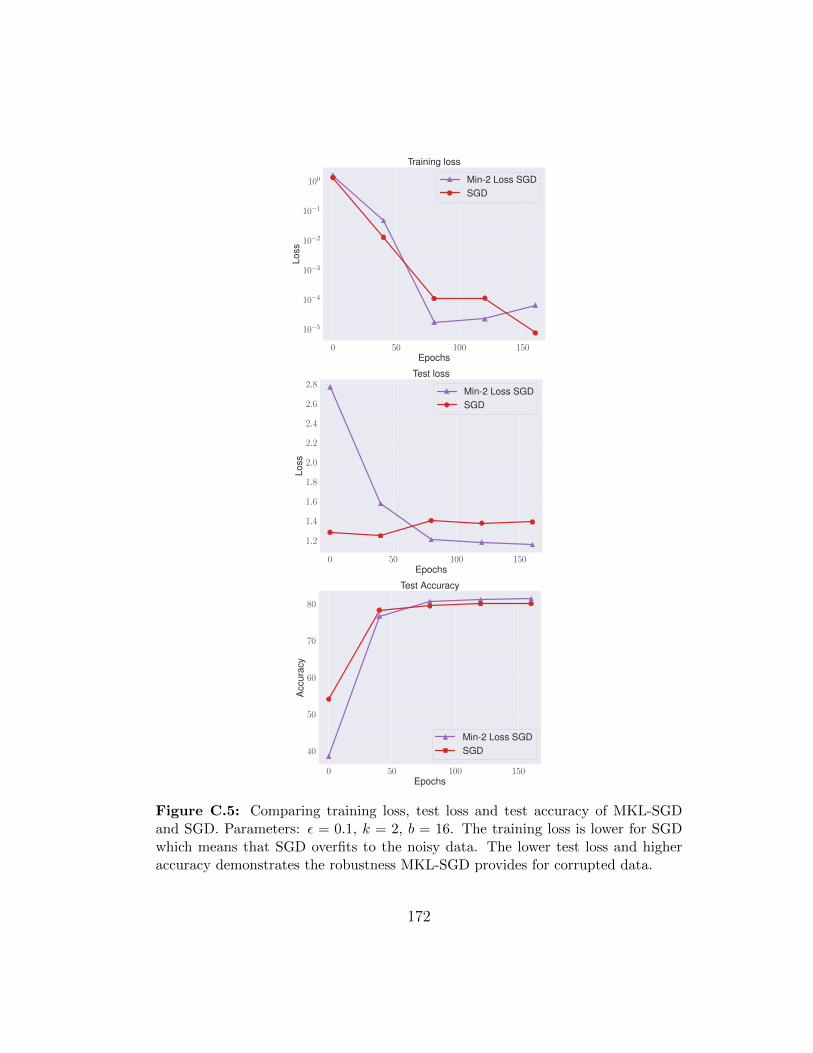
0 50 100 150Epochs
10−5
10−4
10−3
10−2
10−1
100
Loss
Training loss
Min-2 Loss SGDSGD
0 50 100 150Epochs
1.2
1.4
1.6
1.8
2.0
2.2
2.4
2.6
2.8
Loss
Test loss
Min-2 Loss SGDSGD
0 50 100 150Epochs
40
50
60
70
80
Acc
urac
y
Test Accuracy
Min-2 Loss SGDSGD
Figure C.5: Comparing training loss, test loss and test accuracy of MKL-SGDand SGD. Parameters: ε = 0.1, k = 2, b = 16. The training loss is lower for SGDwhich means that SGD overfits to the noisy data. The lower test loss and higheraccuracy demonstrates the robustness MKL-SGD provides for corrupted data.
172

0 50 100 150Epochs
10−5
10−4
10−3
10−2
10−1
100
Loss
Training loss
Min-2 Loss SGDSGD
0 50 100 150Epochs
1.4
1.6
1.8
2.0
2.2
2.4
Loss
Test loss
Min-2 Loss SGDSGD
0 50 100 150Epochs
35
40
45
50
55
60
65
70
Acc
urac
y
Test Accuracy
Min-2 Loss SGDSGD
Figure C.6: Comparing training loss, test loss and test accuracy of MKL-SGDand SGD. Parameters: ε = 0.3, k = 2, b = 16. The training loss is lower for SGDwhich means that SGD overfits to the noisy data. The lower test loss and higheraccuracy demonstrates the robustness MKL-SGD provides for corrupted data.
173

Dataset MNIST with 2-layer CNN (Directed Noise)Optimizer SGD MKL-SGD Oracle
εα 1.0 0.9 0.8 0.7 0.6 0.5 1.00.1 96.76 97.23 95.89 97.47 96.34 94.54 98.520.2 92.54 95.81 95.58 97.46 97.03 95.76 98.330.3 85.77 91.56 93.59 95.30 96.54 95.96 98.160.4 71.95 78.68 82.25 85.93 91.29 94.20 97.98
Table C.1: In this experiments, we train a standard 2 layer CNN on subsampledMNIST (5000 training samples with labels corrupted using random label noise).We train over 80 epochs using an initial learning rate of 0.05 with the decayingschedule of factor 5 after every 30 epochs. The reported accuracy is based on thetrue validation set. The results of the MNIST dataset are reported as the mean of5 runs. For the MKL-SGD algorithm, we introduce a more practical variant thatevaluates k sample losses and picks a batch of size αk where k = 10.
Dataset MNIST with 2-layer CNN (Random Noise)Optimizer SGD MKL-SGD Oracle
εα
1.0 0.9 0.8 0.7 0.6 0.5 1.0
0.1 96.91 97.9 98.06 97.59 96.49 94.43 98.440.2 93.94 95.5 96.16 97.02 97.04 96.25 98.180.3 87.14 90.71 91.60 92.97 94.54 95.36 97.80.4 71.83 74.31 76.6 78.30 77.58 80.86 97.16
Table C.2: In this experiments, we train a standard 2 layer CNN on subsampledMNIST (5000 training samples with labels corrupted using random label noise).We train over 80 epochs using an initial learning rate of 0.05 with the decayingschedule of factor 5 after every 30 epochs. The reported accuracy is based on thetrue validation set. The results of the MNIST dataset are reported as the mean of5 runs. For the MKL-SGD algorithm, we introduce a more practical variant thatevaluates k sample losses and picks a batch of size αk where k = 10.
174

Dataset CIFAR-10 with Resnet-18 (Directed Noise)Optimizer SGD MKL-SGD Oracle
εα
1.0 0.9 0.8 0.7 0.6 0.5 1.0
0.1 79.1 77.52 79.57 81.00 81.94 80.53 84.560.2 72.29 69.58 70.17 72.76 77.77 78.93 84.400.3 63.96 61.43 60.46 61.58 66.49 69.57 84.660.4 52.4 51.53 51.04 51.07 53.57 51.2 84.42
Table C.3: In this experiments, we train Resnet 18 on CIFAR-10 (50000 trainingsamples with labels corrupted using directed label noise). We train over 200 epochsusing an initial learning rate of 0.05 with the decaying schedule of factor 5 after every90 epochs. The reported accuracy is based on the true validation set. The resultsof the CIFAR-10 dataset are reported as the mean of 3 runs. For the MKL-SGDalgorithm, we introduce a more practical variant that evaluates k sample losses andpicks a batch of size αk where k = 16.
175

Appendix D
Balancing SGD
D.1 Proof of Proposition 5.4.2
Theorem D.1.1. Suppose the Loss function defined in (5.5). Assume that
the estimator w close to stationary points satisfying for some finite b ∀i,∃ε
such that
yix>i w
(d) ≥ log
(1
ε
)and e−yi(x
>i w
(d)+b) < 1.
Then ∂L(w)∂b|[]w = w = 0 implies
b ∝ 1
2log
( ∑i∈S1 e
−yix>i w(d)∑
i∈S−1e−yix
>i w
(d)
)(D.1)
Proof. First, we look at the gradient
∂L(w)
∂b=− 1
n
n∑i=1
σ(yi(x>i w + b
))e−yi(x
>i w+b)yi
=1
n
(∑i∈S0
−yie−yi(x>i w(d)+b)
1 + e−yi(x>i w
(d)+b)+∑i∈S1
−yie−yi(x>i w(d)+b)
1 + e−yi(x>i w
(d)+b)
)(D.2)
There exists a small ε for all i such that yix>i w
(d) ≥ log(
1ε
)and e−yi(x
>i w
(d)+b) <
176
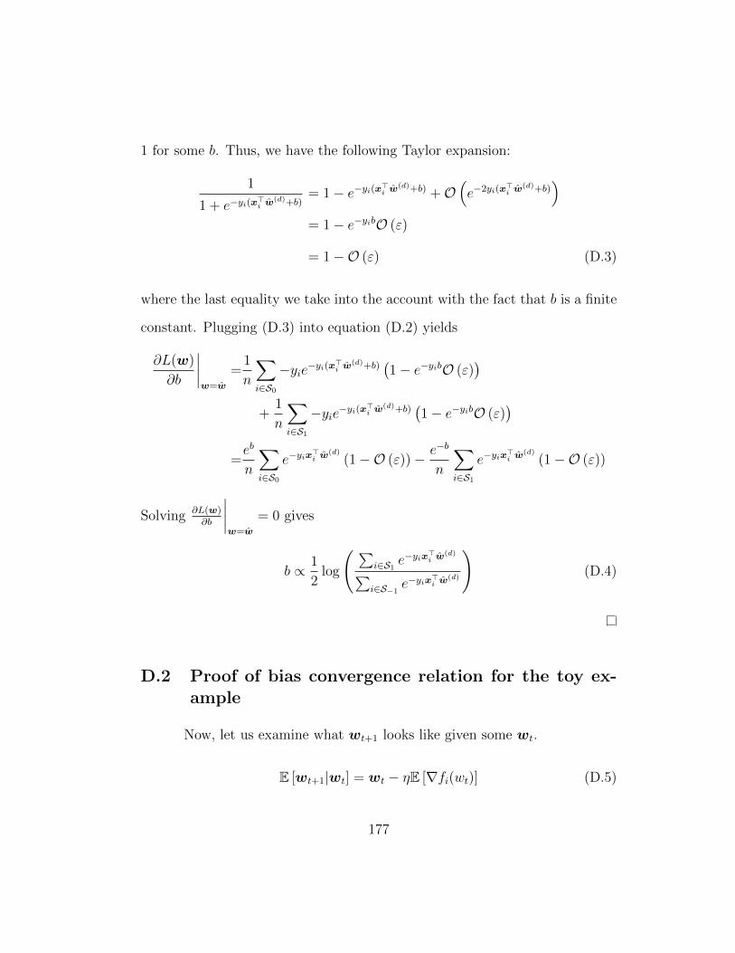
1 for some b. Thus, we have the following Taylor expansion:
1
1 + e−yi(x>i w
(d)+b)= 1− e−yi(x>i w(d)+b) +O
(e−2yi(x
>i w
(d)+b))
= 1− e−yibO (ε)
= 1−O (ε) (D.3)
where the last equality we take into the account with the fact that b is a finite
constant. Plugging (D.3) into equation (D.2) yields
∂L(w)
∂b
∣∣∣∣w=w
=1
n
∑i∈S0
−yie−yi(x>i w
(d)+b)(1− e−yibO (ε)
)+
1
n
∑i∈S1
−yie−yi(x>i w
(d)+b)(1− e−yibO (ε)
)=eb
n
∑i∈S0
e−yix>i w
(d)
(1−O (ε))− e−b
n
∑i∈S1
e−yix>i w
(d)
(1−O (ε))
Solving ∂L(w)∂b
∣∣∣∣w=w
= 0 gives
b ∝ 1
2log
( ∑i∈S1 e
−yix>i w(d)∑
i∈S−1e−yix
>i w
(d)
)(D.4)
D.2 Proof of bias convergence relation for the toy ex-ample
Now, let us examine what wt+1 looks like given some wt.
E [wt+1|wt] = wt − ηE [∇fi(wt)] (D.5)
177

The expected gradient for this toy example at wt = [at, bt]> is given as:
E [∇fi(wt)] = −p1σ(−w>t p1) +∑i∈S−1
xiσ(w>t xi)
≈ −p1σ(−w>t p1) +
∫ 1
0
xiσ(w>t xi)∂xi[0] ... assuming small r
≈ −p1σ(−w>t p1) +
[δ
(w)t
δ(b)t
]
where δ(w)t = 1
atlog exp(at+bt)+1
exp(at)+1and
δ(b)t = 1
a2t(log at(exp(at + bt) + exp(2bt)) + Li2(− exp(at + bt))− Li2(− exp(bt)))
This leads us to two phases of running any SGD based algorithm on
separable data: i) Rapid correction in the direction of wt, ii) Increase in
the magnitude of wt. In general, equation (5.7) indicates that the frequent
occurrence of gradient updates from the majority class than the minority push
the separating hyper-plane further away from majority class. The farther the
separating hyper-plane from the majority class, the smaller (and less useful)
are the corresponding gradient updates from majority class. We know from
[117, 118] that the rate of convergence is quite slow in Phase 2. However, if
we restrict the subset associated with the denominator in equation (5.7), it is
possible to reduce this bias term even further which in turn will lead to faster
convergence.
Using the expected gradient from the toy example, we observe that
while it is easy to see that the bias can affect generalization, it also leads to
slow convergence. High value of bias, bt ensures that the δ(w)t can scale up-to
two times 1at
causing the expected gradient to keep on getting biased until at
178

is not large enough. Thus in the initial phase, when at is small, bias can be
quite high. Only in the second phase when at increases in magnitude does the
bias becomes small. In this paper, we want our proposed algorithm to reach
Phase 2 with as little bias as possible, similar to the case when it would have
received equal distribution of both classes. Similar to
D.3 Convergence
Lemma D.3.1. (Stochastic PAUM in [114]) Consider the perceptron algo-
rithm (Algorithm 6) with the linear classifier
fi(w) = sign(〈w,xi〉) with ‖xi‖2 = 1
and so the ∇wfi(w) = −yixi. Suppose there exits w∗ ∈ Rd such that ‖w∗‖ = 1
and γ(w∗,S0,S1) ≥ Γ. Then the number of updates made by the PAUM is
bounded w.h.p. by
1
Γ2+
2(1− r)τ−1 + 2rτ1
ηΓ2(D.6)
Proof. Observe that
‖wt+1‖2 = ‖wt‖2 + 2ηyi〈wt, xi〉1i∈S0 + 2ηyi〈wt, xi〉1i∈S1 + η2‖xi‖2
E[‖wt+1‖2
]≤ E
[‖wt‖2
]+ 2ητ−1E[1i∈S0 ] + 2ητ1E[1i∈S1 ] + η2‖xi‖2
= E[‖wt‖2
]+ 2η(1− r)τ−1 + 2ηrτ1 + η2 take ‖xi‖2 = 1
(E[‖wt+1‖])2 ≤ E[‖wt+1‖2
]≤ 2tη(1− r)τ−1 + 2ηrτ1 + η2t
179

Algorithm 6 Stochastic PAUM (the minority class y = 1)
1: Initialize w. Two margin parameters τ−1 and τ1
2: Given samples D = (xi, yi)∞i=1
3: for t = 1 to m do4: Chose i uniformly from 1, . . . , n.5: if yiw
>xi ≤ τyi then6: w+ = w + ηyixi7: end if8: end for9: Return w
On the other hand, we have
〈E[wt+1],w∗〉 = 〈E[wt],w∗〉+ ηE[yi〈xi,w∗〉]
≥ 〈E[wt],w∗〉+ ηΓ
≥ tηΓ
Thus, we have
(tηΓ)2 ≤ (〈E[wt+1],w∗〉)2
≤ ‖E[wt+1]‖2‖w∗‖2
≤ 2ηt(1− r)τ−1 + 2ηrtτ1 + η2t
which is upper bound (D.6)
Theorem D.3.2 (Restatement of Theorem 5.4.3). Consider the B-SGD algo-
rithm with fixed thresholds (over time) τ−1 and τ1 for the majority and minority
class, respectively. The expected gradient update step for B-SGD is as follows:
E [wt+1|wt] = wt − η∇fi(wt)Ifi(wt)≥Cyi (D.7)
180

Suppose the data is normalized (i.e., ‖xi‖ = 1). Define the margin
γ(w,S−1,S1) := mini
yi (〈w,xi〉)‖w‖ .
Suppose there exists w∗ ∈ Rd+1 such that ‖w∗‖ = 1 and γ(w∗,S−1,S1) ≥ Γ.
Then the number of gradient updates performed by Algorithm 3 is bounded
w.h.p. by
1
Γ2 ((1− r)β−1 + rβ1)2 +2(1− r)B−1 + 2rB1
ηΓ2 ((1− r)β−1 + rβ1)2 (D.8)
where βyi = (exp(Cyi)− 1) exp(−Cyi) and Byi = − log (exp(Cyi)− 1).
Note that here Cyi is τyi in Theorem 5.4.3.
Proof. Let pi(wt) = exp(−yi〈w,xi〉)1+exp(−yi〈w,xi〉) . Note that
log(1 + exp (−yi〈w,xi〉)) ≥ Cyi ⇔ yi〈w,xi〉 ≤ − log (exp(Cyi)− 1)︸ ︷︷ ︸τyi
⇒ (exp(Cyi)− 1) exp(−Cyi)︸ ︷︷ ︸βyi
≤ pi(wt) ≤ 1
Observe that
‖wt+1‖2 = ‖wt‖2 + 2ηyi〈wt, xi〉pi(wt)1i∈S0
+ 2ηyi〈wt, xi〉pi(wt)1i∈S1 + η2‖pi(wt)xi‖2
E[‖wt+1‖2] ≤ E[‖wt‖2] + 2η(1− r)B−1 + 2rηB1 + η2‖xi‖2
181

On the other hand, we have
〈E[wt+1],w∗〉 = 〈E[wt],w∗〉+ ηE[pi(wt)yi〈xi,w∗〉]
≥ 〈E[wt],w∗〉+ ηβ−1E[1i∈S−1 ]Γ + ηβ1E[1i∈S1 ]Γ
≥ 〈E[wt],w∗〉+ ((1− r)β−1 + rβ1) ηΓ
≥ tη ((1− r)β−1 + rβ1) Γ
Thus, we have
(tηΓ ((1− r)β−1 + rβ1))2 ≤ (〈E[wt+1],w∗〉)2
≤ ‖E[wt+1]‖2‖w∗‖2
≤ 2ηt(1− r)B−1 + 2ηrtB1 + η2t
which yields our upper bound of t
D.4 Proof of Proposition 5.4.4
Proposition D.4.1. Suppose the data is normalized (i.e., ‖xi‖ = 1). Suppose
w minimizes both equations (5.10) and (5.11), then without loss of generality
w>xi < 0,∀i ∈ S−1. Set τ−1 ≥ 0 for the set Aw. Solving for τ−1 given some
r in equation (5.12), we observe that τ−1 > 0 is monotonically decreasing
function with respect to r ∈ [0, 0.5]. In addition, If r → 0.5 or r1−r → 1, then
τ−1 → 0. If r → 0 or r1−r → 0, then we could let τ−1 → log(1 + exp(‖w‖)) so
that we have 1log(1+e−zi)>τ−1 = 0. 1
1Note the the term of τ−1 → log(1 + exp(‖w‖)) is a sufficient condition but not a nec-essary condition. As long as it is greater than c log(1 + exp(〈w,xi〉)) for each i with somec > 1.
182

Proof. The expression that establishes the relation of τ−1 and r is∑i∈S−1
(r
1− r − 1i∈Aw
)∇fi(w)|[
]w = w = 0 (D.9)
Let us now explicitly write down down the function f , ∇f and Aw for the
majority class y = −1:
f(yi = −1, yi) = log(1 + e〈w,xi〉
)∇wf(yi = −1, yi) =
xi1 + exp (−〈w,xi〉)
Aw =i ∈ S−1
∣∣ log(1 + e〈w,xi〉
)> τ−1
=i ∈ S−1
∣∣− 〈w,xi〉 ≤ − log (eτ−1 − 1)
Substituting above equations back to (D.9) gives
r
1− r∑i∈S−1
xi1 + exp (−〈w,xi〉)
=∑i∈S−1
xi1i∈Aw
1 + exp (−〈w,xi〉)
For the class i ∈ S−1, we have 〈w,xi〉 < 0, multiplying above with w, we get
r
1− r∑i∈S−1
−〈w,xi〉1 + exp (−〈w,xi〉)
=∑i∈S−1
−〈w,xi〉1log(1 + e〈w,xi〉
)> τ−1
1 + exp (−〈w,xi〉)
⇒ r
1− r∑i∈S−1
zi1 + exp (zi)
=∑i∈S−1
zi1log (1 + e−zi) > τ−11 + exp (zi)
(D.10)
where let zi = −〈w,xi〉 > 0. Now observe that when r increases, the left
hand side of the above equation will increases since the term∑
i∈S−1
zi1+exp(zi)
is fixed. For the right hand side, when τ−1 decreases with other parameters
fixed, the term∑
i∈S−1
zi1log(1+e−zi)>τ−11+exp(zi)
increases. Thus when r increase, τ−1
needs to decrease for the equality (D.10) to hold. Finally, it is easy to check
that
183
• If r → 0.5 or r1−r → 1, τ−1 → 0;
• If r → 0 or r1−r → 0 , then 1log (1 + e−zi) > τ−1 = 0. A sufficient
condition for 1log (1 + e−zi) > τ−1 = 0 is τ−1 = log(1 + e‖w‖
)for
normalized data (i.e., ‖xi‖ = 1).
D.5 Experiments
We performed a grid-based hyper-parameter search for initial learning
rates for SGD and picked the step-size that achieves the lowest training loss for
SGD (Note that B-SGD had no learning rate based hyper-parameter tuning).
While the training dataset was imbalanced, the test loss was evaluated over
a balanced test set. The following table illustrates the training and test loss
performance of SGD and B-SGD vs. the number of gradient computations. It
is quite evident that B-SGD achieves significant performance gains in terms
of both loss and number of gradient computations over its SGD counterpart.
D.5.1 Synthetic experiments
In this section, we run synthetic experiments on logistic regression on
separable data. We assume that the training data is imbalanced however the
test distribution is balanced. In this section, we compare the performance of
SGD and B-SGD in terms of training error, test error and estimation error vs
gradient computations (and time taken) for different values of d. We observe
184

that SGD has high estimation errors demonstrating that it over-fits to the
majority class. On the other hand, B-SGD has low estimation error, thus
demonstrating its effectiveness in imbalanced classification.
Algorithm SGD B-SGD Focal
Dataset TL TEL TA GC TL TEL TA GC TA
car eval 4 0.031 0.247 88.1 8.64 · e4 0.278 0.249 89.3 9.98 · e3 89.2optical digits 0.054 0.387 89.0 1.41 · e5 1.479 0.367 89.6 8.11 · e3 88.0isolet 0.035 0.649 87.0 1.94 · e5 0.485 0.585 88.5 8.80 · e3 88.4letter img 0.061 0.66 83.8 2.00 · e5 1.81 0.612 83.8 3.34 · e3 84.3pen digits 0.097 0.388 83.8 2.74 · e5 0.711 0.364 85.1 3.33 · e4 85.1mammography 0.051 0.901 70.9 5.59 · e4 0.144 0.873 70.5 2.12 · e3 71.1
Table D.1: Comparing training loss (TL), Test Loss (TEL), Test AUC (TA), Top-1Test Error (TE1), and Number of gradient computations (GC) for SGD and B-SGDover different Imbalanced datasets. The reported results for the first 6 datasets arean average of 5 runs, and for the last 3 datasets are an average of 3 runs. Focalloss (Focal) is the state-of-the-art method proposed in [2], which changes the lossfunction and so it is not fair to compare the training and the test errors. Focalhas the same number of gradient computations as SGD. Hence, we only report testaccuracy for Focal.
D.5.2 Real data from imblearn package
We ran some of the experiments described in Table ?? on more datasets
and for more iterations and tabulated the results in Table 5.1. Using the
same setup as described in the main paper, we run experiments on additional
datasets in the imblearn package and further illustrate that using B-SGD re-
duces the number of gradient computations required as well as improves the
generalization performance. To generate the training test split, we use strat-
ified sampling and ensure that the ratio of the number of samples for the
185

0 20000 40000 60000 80000Number of gradient computations
101
100
Est
imat
ion
Err
or, |
|ww
* ||
Imbalanced Labels (frac = 0.0126, d = 20)
SGDBalancing SGD
2.5 5.0 7.5 10.0 12.5 15.0 17.5Time taken (in seconds)
101
100
Est
imat
ion
Err
or, |
|ww
* ||
Imbalanced Labels (frac = 0.0126, d = 20)
SGDBalancing SGD
Figure D.1: Comparing the training loss and test loss vs the number of gra-dient computations for SGD and Balancing SGD for synthetic datasets acrossd = 10, 20, 50
186

minority class in the training and test set is 3:1. We then randomly sample
data from the majority class such that the number of training and test points
are identical. Thus, the test set often comprises of around 3 − 5% of the
training set depending on the imbalance ratio r. Further information about
the datasets including the number of samples, number of feature per samples
and the true imbalance ratio is available in the sklearn documentation of the
imblearn package [157].
For a given run, we pass the same samples through SGD, B-SGD and
Focal Loss. B-SGD evaluates the loss of the incoming samples and determines
whether to take an update step while the other two algorithms always take an
update step. For evaluation purposes we take the average of 3 runs and calcu-
late the expected moving average of training loss, test loss and test AUC with
parameter value of 0.01 for the most recent evaluation. However, label distri-
bution aware methods often show better generalization than B-SGD, however,
over significantly more gradient computations.
Lastly, we observe that the variance in training data is high as we train
over only one sample at a time. This variance term can be reduced by taking
a mini-batch, which is also a practical alternative for large datasets.
D.5.3 Artificially generated imbalanced datasets from real data
D.5.3.1 Hyperparameter Tuning:
For hyper-parameter tuning, we vary the step size as (η ∈ 0.1, 0.01, 0.001).
Similarly, we use the following step-size decay rule ηt = η1+q·t where q ∈
187

100 101 102 103 104 105
Number of iterations
2
4
6
8
10
12Te
st L
oss
Test loss for isolet with r=0.0834SGDBSGD
100 101 102 103 104 105
Number of iterations
50
60
70
80
90
Test
AUC
(%)
Test AUC for isolet with r=0.0834SGDBSGDFocal Loss
100 101 102 103 104 105
Number of iterations
0.3
0.4
0.5
0.6
0.7
Test
Los
s
Test loss for optical_digits with r=0.1094SGDBSGD
100 101 102 103 104 105
Number of iterations
70
75
80
85
90
Test
AUC
(%)
Test AUC for optical_digits with r=0.1094SGDBSGDFocal Loss
100 101 102 103 104 105
Number of iterations
0.4
0.5
0.6
0.7
0.8
Test
Los
s
Test loss for pen_digits with r=0.1062SGDBSGD
100 101 102 103 104 105
Number of iterations
65
70
75
80
85
Test
AUC
(%)
Test AUC for pen_digits with r=0.1062SGDBSGDFocal Loss
Figure D.2: Comparing the training loss and test loss vs the number of gradientcomputations for SGD and Balancing SGD for isolet, optical digits and pen digitsdataset. Each experiment is an average of 5 runs
188

Algorithm SGD B-SGD Focal
TL TEL TE1 Epochs TL TEL TE1 Epochs TE1
CIFAR-10 0.021 1.43 28.5 200 0.163 0.90 26.2 88 28.7
Table D.2: Comparing training loss (TL), Test Loss (TEL), Test AUC (TA), Top-1 Test Error (TE1), and Number of gradient computations (GC) for SGD and B-SGD over different Imbalanced datasets. The reported results artificially generatedimbalanced dataset for CIFAR-10. Focal loss (Focal) is the state-of-the-art methodproposed in [2], which changes the loss function and so it is not fair to compare thetraining and the test errors. Focal has the same number of gradient computationsas SGD. Hence, we only report test accuracy for Focal.
0.1, 0.01, 0.001 and select the hyperparameter tuple that optimizes SGD and
Focal individually. For B-SGD, the threshold parameter was tuned over the
following set, c ∈ 0.1, 0.2, 0.5, 1.
D.5.4 CIFAR-10
We use the experimental setup in [12] and evaluated and compared the
performance of B-SGD with respect to SGD and Focal Loss. We observe that
in this case also, B-SGD outperforms SGD and Focal Loss in terms of both
gradient evaluations and generalization performance. Note, that our method
typically outperforms or shows comparable performance to many state of the
art methods which are not label distribution aware.
D.5.5 Early Stopping:
Early stopping is a beneficial way to achieve a solution that generalizes
well. Initially, the bias reduction caused by B-SGD allows w to get closer to
w∗. However, if we run the algorithm for too long, then the algorithm starts
189

getting closer and closer to w that determines the separating hyper-plane of
the training data and away from w∗, which in turn decreases the magnitude
of improvements achieved by B-SGD over SGD.
D.5.6 Parameter Sensitivity of Threshold Parameter, c
Figure D.3: In this figure, we evaluate the parameter sensitivity of thresholdparameter c in Algorithm 3 with respect to the training error, test error and numberof gradient computations. We observe that the number of gradient computations isinversely proportional to threshold, while both training and test loss first decreaseand then increase as c increases from 0 to 50
The dependence of the generalization behavior (and the number of
gradient steps taken) follows a linear increasing behavior up to a particular
value beyond which it becomes constant. For c = 0, the loss threshold function
accepts all samples, and B-SGD is identical to SGD. As c increases, B-SGD
190

starts selectively choosing samples from the majority class leading to gradual
improvements in generalization and convergence performance with respect to
SGD. However, as c > c′ for some c′, it is observed that fewer and fewer samples
are accepted from majority class until they are not enough to determine the
supporting hyper-plane, in turn adversely impacting both generalization and
convergence performances. For larger values of c, the generalization will often
be worse than SGD. As a result, low values of c, i.e., c = 1,are recommended
in practice. We also argue that for B-SGD hyper-parameter tuning over c is
more important than over learning rate η.
191

Appendix E
Conclusions
In this dissertation, we propose practical variants of SGD to address
its shortcomings with respect to convergence, generalization and robustness.
192

Bibliography
[1] Causality workbench team. A phamacology dataset, 06 2008.
[2] Tsung-Yi Lin, Priya Goyal, Ross Girshick, Kaiming He, and Piotr Dollar.
Focal loss for dense object detection. In Proceedings of the IEEE inter-
national conference on computer vision, pages 2980–2988, 2017.
[3] Rie Johnson and Tong Zhang. Accelerating stochastic gradient descent
using predictive variance reduction. In Advances in Neural Information
Processing Systems, pages 315–323, 2013.
[4] Lin Xiao and Tong Zhang. A proximal stochastic gradient method
with progressive variance reduction. SIAM Journal on Optimization,
24(4):2057–2075, 2014.
[5] K. He, X. Zhang, S. Ren, and J. Sun. Identity mappings in deep residual
networks. In European Conference on Computer Vision, pages 630–645.
Springer, 2016.
[6] A. Howard, M. Zhu, B. Chen, D. Kalenichenko, W. Wang, T. Weyand,
M. Andreetto, and H. Adam. MobileNets: Efficient convolutional neural
networks for mobile vision applications. arXiv preprint arXiv:1704.04861,
2017.
193

[7] M. Sandler, A. Howard, M. Zhu, A. Zhmoginov, and L.-C. Chen. In-
verted residuals and linear bottlenecks: Mobile networks for classifica-
tion, detection and segmentation. arXiv preprint arXiv:1801.04381,
2018.
[8] Jia Deng, Wei Dong, Richard Socher, Li-Jia Li, Kai Li, and Li Fei-Fei.
Imagenet: A large-scale hierarchical image database. In 2009 IEEE
conference on computer vision and pattern recognition, pages 248–255.
Ieee, 2009.
[9] Nitesh V Chawla, Kevin W Bowyer, Lawrence O Hall, and W Philip
Kegelmeyer. Smote: synthetic minority over-sampling technique. Jour-
nal of artificial intelligence research, 16:321–357, 2002.
[10] Haibo He, Yang Bai, Edwardo A Garcia, and Shutao Li. Adasyn: Adap-
tive synthetic sampling approach for imbalanced learning. In 2008 IEEE
international joint conference on neural networks (IEEE world congress
on computational intelligence), pages 1322–1328. IEEE, 2008.
[11] Haibo He and Yunqian Ma. Imbalanced learning: foundations, algo-
rithms, and applications. John Wiley & Sons, 2013.
[12] Kaidi Cao, Colin Wei, Adrien Gaidon, Nikos Arechiga, and Tengyu Ma.
Learning imbalanced datasets with label-distribution-aware margin loss.
arXiv preprint arXiv:1906.07413, 2019.
194

[13] Vatsal Shah, Megasthenis Asteris, Anastasios Kyrillidis, and Sujay Sang-
havi. Trading-off variance and complexity in stochastic gradient descent.
arXiv preprint arXiv:1603.06861, 2016.
[14] Ruiliang Zhang, Shuai Zheng, and James T Kwok. Fast distributed
asynchronous sgd with variance reduction. arXiv preprint arXiv:1508.01633,
2015.
[15] Mark Schmidt and Nicolas Le Roux. Fast convergence of stochas-
tic gradient descent under a strong growth condition. arXiv preprint
arXiv:1308.6370, 2013.
[16] Aaron Defazio, Francis Bach, and Simon Lacoste-Julien. Saga: A fast
incremental gradient method with support for non-strongly convex com-
posite objectives. In Advances in Neural Information Processing Sys-
tems, pages 1646–1654, 2014.
[17] Shai Shalev-Shwartz and Tong Zhang. Stochastic dual coordinate as-
cent methods for regularized loss. The Journal of Machine Learning
Research, 14(1):567–599, 2013.
[18] Jeffrey Dean, Greg Corrado, Rajat Monga, Kai Chen, Matthieu Devin,
Mark Mao, Andrew Senior, Paul Tucker, Ke Yang, and Quoc V Le.
Large scale distributed deep networks. In Advances in Neural Informa-
tion Processing Systems, pages 1223–1231, 2012.
195

[19] Nicolas L Roux, Mark Schmidt, and Francis R Bach. A stochastic
gradient method with an exponential convergence rate for finite training
sets. In Advances in Neural Information Processing Systems, pages
2663–2671, 2012.
[20] Guillaume Bouchard, Theo Trouillon, Julien Perez, and Adrien Gaidon.
Accelerating stochastic gradient descent via online learning to sample.
arXiv preprint arXiv:1506.09016, 2015.
[21] Christopher D Sa, Christopher Re, and Kunle Olukotun. Global conver-
gence of stochastic gradient descent for some non-convex matrix prob-
lems. In Proceedings of the 32nd International Conference on Machine
Learning (ICML-15), pages 2332–2341, 2015.
[22] Yurii Nesterov. Introductory lectures on convex optimization, volume 87.
Springer Science & Business Media, 2004.
[23] Stephen Boyd and Lieven Vandenberghe. Convex optimization. Cam-
bridge university press, 2004.
[24] Herbert Robbins and Sutton Monro. A stochastic approximation method.
The annals of mathematical statistics, pages 400–407, 1951.
[25] Leon Bottou. Large-scale machine learning with stochastic gradient
descent. In Proceedings of COMPSTAT’2010, pages 177–186. Springer,
2010.
196

[26] Jakub Konecny and Peter Richtarik. Semi-stochastic gradient descent
methods. arXiv preprint arXiv:1312.1666, 2013.
[27] Jakub Konevcny, Jie Liu, Peter Richtarik, and Martin Takac. ms2gd:
Mini-batch semi-stochastic gradient descent in the proximal setting. arXiv
preprint arXiv:1410.4744, 2014.
[28] Jiquan Ngiam, Adam Coates, Ahbik Lahiri, Bobby Prochnow, Quoc V
Le, and Andrew Y Ng. On optimization methods for deep learning. In
Proceedings of the 28th International Conference on Machine Learning
(ICML-11), pages 265–272, 2011.
[29] Ilya Sutskever, James Martens, George Dahl, and Geoffrey Hinton. On
the importance of initialization and momentum in deep learning. In
Proceedings of the 30th international conference on machine learning
(ICML-13), pages 1139–1147, 2013.
[30] Martin Zinkevich, Markus Weimer, Lihong Li, and Alex J Smola. Par-
allelized stochastic gradient descent. In Advances in neural information
processing systems, pages 2595–2603, 2010.
[31] Mark Schmidt. Convergence rate of stochastic gradient with constant
step size, Sep 2014.
[32] Angelia Nedic and Dimitri Bertsekas. Convergence rate of incremen-
tal subgradient algorithms. In Stochastic optimization: algorithms and
applications, pages 223–264. Springer, 2001.
197

[33] Dimitri P Bertsekas. Incremental gradient, subgradient, and proximal
methods for convex optimization: A survey. Optimization for Machine
Learning, 2010:1–38, 2011.
[34] Aaron J Defazio, Tiberio S Caetano, and Justin Domke. Finito: A
faster, permutable incremental gradient method for big data problems.
arXiv preprint arXiv:1407.2710, 2014.
[35] Julien Mairal. Optimization with first-order surrogate functions. arXiv
preprint arXiv:1305.3120, 2013.
[36] Zeyuan Allen-Zhu and Yang Yuan. Univr: A universal variance reduc-
tion framework for proximal stochastic gradient method. arXiv preprint
arXiv:1506.01972, 2015.
[37] Sashank J Reddi, Ahmed Hefny, Suvrit Sra, Barnabas Poczos, and Alex
Smola. On variance reduction in stochastic gradient descent and its
asynchronous variants. arXiv preprint arXiv:1506.06840, 2015.
[38] Jason Lee, Tengyu Ma, and Qihang Lin. Distributed stochastic variance
reduced gradient methods. arXiv preprint arXiv:1507.07595, 2015.
[39] Dimitri P Bertsekas. Nonlinear programming. Journal of the Opera-
tional Research Society, 48(3):334–334, 1997.
[40] Mikhail V Solodov. Incremental gradient algorithms with stepsizes
bounded away from zero. Computational Optimization and Applica-
tions, 11(1):23–35, 1998.
198

[41] Paul Tseng. An incremental gradient (-projection) method with momen-
tum term and adaptive stepsize rule. SIAM Journal on Optimization,
8(2):506–531, 1998.
[42] Vatsal Shah, Anastasios Kyrillidis, and Sujay Sanghavi. Minimum
weight norm models do not always generalize well for over-parameterized
problems. arXiv preprint arXiv:1811.07055, 2018.
[43] Peter L Bartlett, Philip M Long, Gabor Lugosi, and Alexander Tsigler.
Benign overfitting in linear regression. Proceedings of the National
Academy of Sciences, 2020.
[44] Vidya Muthukumar, Kailas Vodrahalli, Vignesh Subramanian, and Anant
Sahai. Harmless interpolation of noisy data in regression. IEEE Journal
on Selected Areas in Information Theory, 2020.
[45] M. Belkin, S. Ma, and S. Mandal. To understand deep learning we need
to understand kernel learning. arXiv preprint arXiv:1802.01396, 2018.
[46] Christopher M Bishop. Pattern recognition and machine learning. springer,
2006.
[47] Jerome Friedman, Trevor Hastie, and Robert Tibshirani. The elements
of statistical learning. Number 10 in 1. Springer series in statistics New
York, 2001.
[48] Shai Shalev-Shwartz and Shai Ben-David. Understanding machine
learning: From theory to algorithms. Cambridge university press, 2014.
199

[49] Zeyuan Allen-Zhu, Yuanzhi Li, and Zhao Song. A convergence theory
for deep learning via over-parameterization. arXiv preprint arXiv:1811.03962,
2018.
[50] Simon S Du, Xiyu Zhai, Barnabas Poczos, and Aarti Singh. Gradient
descent provably optimizes over-parameterized neural networks. arXiv
preprint arXiv:1810.02054, 2018.
[51] Simon S Du and Jason D Lee. On the power of over-parametrization in
neural networks with quadratic activation. arXiv preprint arXiv:1803.01206,
2018.
[52] Y. Bengio. Practical recommendations for gradient-based training of
deep architectures. In Neural networks: Tricks of the trade, pages 437–
478. Springer, 2012.
[53] L. Bottou. Stochastic gradient descent tricks. In Neural networks:
Tricks of the trade, pages 421–436. Springer, 2012.
[54] G. Orr and K.-R. Muller. Neural networks: tricks of the trade. Springer,
2003.
[55] Chiyuan Zhang, Samy Bengio, Moritz Hardt, Benjamin Recht, and Oriol
Vinyals. Understanding deep learning requires rethinking generaliza-
tion. arXiv preprint arXiv:1611.03530, 2016.
[56] T. Schaul, S. Zhang, and Y. LeCun. No more pesky learning rates. In
International Conference on Machine Learning, pages 343–351, 2013.
200

[57] W. Xu. Towards optimal one pass large scale learning with averaged
stochastic gradient descent. arXiv preprint arXiv:1107.2490, 2011.
[58] A. Senior, G. Heigold, and K. Yang. An empirical study of learning rates
in deep neural networks for speech recognition. In Acoustics, Speech and
Signal Processing (ICASSP), 2013 IEEE International Conference on,
pages 6724–6728. IEEE, 2013.
[59] Sebastian Ruder. An overview of gradient descent optimization algo-
rithms. arXiv preprint arXiv:1609.04747, 2016.
[60] J. Duchi, E. Hazan, and Y. Singer. Adaptive subgradient methods
for online learning and stochastic optimization. Journal of Machine
Learning Research, 12(Jul):2121–2159, 2011.
[61] D. Kingma and J. Ba. Adam: A method for stochastic optimization.
arXiv preprint arXiv:1412.6980, 2014.
[62] M. Zeiler. ADADELTA: an adaptive learning rate method. arXiv
preprint arXiv:1212.5701, 2012.
[63] T. Tieleman and G. Hinton. Lecture 6.5-RMSPro: Divide the gradient
by a running average of its recent magnitude. COURSERA: Neural
networks for machine learning, 4(2):26–31, 2012.
[64] T. Dozat. Incorporating Nesterov momentum into Adam. In Interna-
tional Conference on Learning Representations, 2016.
201

[65] J. Zhang and I. Mitliagkas. YellowFin and the art of momentum
tuning. arXiv preprint arXiv:1706.03471, 2017.
[66] S. Gunasekar, J. Lee, D. Soudry, and N. Srebro. Characterizing implicit
bias in terms of optimization geometry. arXiv preprint arXiv:1802.08246,
2018.
[67] Trevor Hastie, Andrea Montanari, Saharon Rosset, and Ryan J Tibshi-
rani. Surprises in high-dimensional ridgeless least squares interpolation.
arXiv preprint arXiv:1903.08560, 2019.
[68] Song Mei and Andrea Montanari. The generalization error of ran-
dom features regression: Precise asymptotics and double descent curve.
arXiv preprint arXiv:1908.05355, 2019.
[69] Phuong Thi Tran et al. On the convergence proof of amsgrad and a new
version. IEEE Access, 7:61706–61716, 2019.
[70] Sashank J Reddi, Satyen Kale, and Sanjiv Kumar. On the convergence
of adam and beyond. arXiv preprint arXiv:1904.09237, 2019.
[71] A. Wilson, R. Roelofs, M. Stern, N. Srebro, and B. Recht. The marginal
value of adaptive gradient methods in machine learning. In Advances in
Neural Information Processing Systems, pages 4151–4161, 2017.
[72] M. S. Nacson, J. Lee, S. Gunasekar, N. Srebro, and D. Soudry. Conver-
gence of gradient descent on separable data. arXiv preprint arXiv:1803.01905,
2018.
202

[73] Y. Nesterov. Introductory lectures on convex optimization: A basic
course, volume 87. Springer Science & Business Media, 2013.
[74] Roger A Horn and Charles R Johnson. Matrix analysis. Cambridge
university press, 2012.
[75] D. Dowler. Bounding the norm of matrix powers, 2013.
[76] Xiaoxia Wu, Simon S Du, and Rachel Ward. Global convergence of
adaptive gradient methods for an over-parameterized neural network.
arXiv preprint arXiv:1902.07111, 2019.
[77] Vidya Muthukumar, Adhyyan Narang, Vignesh Subramanian, Mikhail
Belkin, Daniel Hsu, and Anant Sahai. Classification vs regression in
overparameterized regimes: Does the loss function matter?, 2020.
[78] M. C. Mukkamala and M. Hein. Variants of RMSProp and AdaGrad
with logarithmic regret bounds. arXiv preprint arXiv:1706.05507, 2017.
[79] Nitish Srivastava, Geoffrey Hinton, Alex Krizhevsky, Ilya Sutskever, and
Ruslan Salakhutdinov. Dropout: A simple way to prevent neural net-
works from overfitting. The Journal of Machine Learning Research,
15(1):1929–1958, 2014.
[80] Kaiming He, Xiangyu Zhang, Shaoqing Ren, and Jian Sun. Deep resid-
ual learning for image recognition. In Proceedings of the IEEE confer-
ence on computer vision and pattern recognition, pages 770–778, 2016.
203

[81] M. Telgarsky. Benefits of depth in neural networks. arXiv preprint
arXiv:1602.04485, 2016.
[82] Christian Szegedy, Wei Liu, Yangqing Jia, Pierre Sermanet, Scott Reed,
Dragomir Anguelov, Dumitru Erhan, Vincent Vanhoucke, and Andrew
Rabinovich. Going deeper with convolutions. In Proceedings of the
IEEE conference on computer vision and pattern recognition, pages 1–9,
2015.
[83] Y. Bansal, M. Advani, D. Cox, and A. Saxe. Minnorm training: an
algorithm for training over-parameterized deep neural networks, 2018.
[84] Samuel L Smith, Pieter-Jan Kindermans, and Quoc V Le. Don’t decay
the learning rate, increase the batch size. arXiv preprint arXiv:1711.00489,
2017.
[85] Vatsal Shah, Xiaoxia Wu, and Sujay Sanghavi. Choosing the sample
with lowest loss makes sgd robust. In Silvia Chiappa and Roberto Calan-
dra, editors, Proceedings of the Twenty Third International Conference
on Artificial Intelligence and Statistics, volume 108 of Proceedings of
Machine Learning Research, pages 2120–2130, Online, 26–28 Aug 2020.
PMLR.
[86] Herman Kahn and Andy W Marshall. Methods of reducing sample
size in monte carlo computations. Journal of the Operations Research
Society of America, 1(5):263–278, 1953.
204
[87] Thomas Strohmer and Roman Vershynin. A randomized kaczmarz al-
gorithm with exponential convergence. Journal of Fourier Analysis and
Applications, 15(2):262, 2009.
[88] Peilin Zhao and Tong Zhang. Stochastic optimization with importance
sampling for regularized loss minimization. In international conference
on machine learning, pages 1–9, 2015.
[89] Angelos Katharopoulos and Francois Fleuret. Not all samples are cre-
ated equal: Deep learning with importance sampling. arXiv preprint
arXiv:1803.00942, 2018.
[90] Deanna Needell, Rachel Ward, and Nati Srebro. Stochastic gradient
descent, weighted sampling, and the randomized kaczmarz algorithm.
In Advances in neural information processing systems, pages 1017–1025,
2014.
[91] Eric Moulines and Francis R Bach. Non-asymptotic analysis of stochas-
tic approximation algorithms for machine learning. In Advances in
Neural Information Processing Systems, pages 451–459, 2011.
[92] Yin Tat Lee and Aaron Sidford. Efficient accelerated coordinate descent
methods and faster algorithms for solving linear systems. In 2013 IEEE
54th Annual Symposium on Foundations of Computer Science, pages
147–156. IEEE, 2013.
205

[93] Yoav Freund, Robert Schapire, and Naoki Abe. A short introduction to
boosting. Journal-Japanese Society For Artificial Intelligence, 14(771-
780):1612, 1999.
[94] Peter J Rousseeuw. Least median of squares regression. Journal of the
American statistical association, 79(388):871–880, 1984.
[95] Jan Visek et al. The least weighted squares ii. consistency and asymp-
totic normality. Bulletin of the Czech Econometric Society, 9, 2002.
[96] Jan Amos Visek. The least trimmed squares. part i: Consistency.
Kybernetika, 42(1):1–36, 2006.
[97] Peter J Huber. Robust statistics. Springer, 2011.
[98] Kush Bhatia, Prateek Jain, and Purushottam Kar. Robust regression
via hard thresholding. In Advances in Neural Information Processing
Systems, pages 721–729, 2015.
[99] Kush Bhatia, Prateek Jain, Parameswaran Kamalaruban, and Purushot-
tam Kar. Consistent robust regression. In Advances in Neural Infor-
mation Processing Systems, pages 2110–2119, 2017.
[100] Yanyao Shen and Sujay Sanghavi. Learning with bad training data via
iterative trimmed loss minimization. In International Conference on
Machine Learning, pages 5739–5748, 2019.
206
[101] Ilias Diakonikolas, Gautam Kamath, Daniel Kane, Jerry Li, Ankur Moitra,
and Alistair Stewart. Robust estimators in high-dimensions without the
computational intractability. SIAM Journal on Computing, 48(2):742–
864, 2019.
[102] Kevin A Lai, Anup B Rao, and Santosh Vempala. Agnostic estimation
of mean and covariance. In 2016 IEEE 57th Annual Symposium on
Foundations of Computer Science (FOCS), pages 665–674. IEEE, 2016.
[103] Moses Charikar, Jacob Steinhardt, and Gregory Valiant. Learning from
untrusted data. In Proceedings of the 49th Annual ACM SIGACT Sym-
posium on Theory of Computing, pages 47–60. ACM, 2017.
[104] Ilias Diakonikolas, Gautam Kamath, Daniel M Kane, Jerry Li, Jacob
Steinhardt, and Alistair Stewart. Sever: A robust meta-algorithm for
stochastic optimization. arXiv preprint arXiv:1803.02815, 2018.
[105] Adarsh Prasad, Arun Sai Suggala, Sivaraman Balakrishnan, and Pradeep
Ravikumar. Robust estimation via robust gradient estimation. arXiv
preprint arXiv:1802.06485, 2018.
[106] Farhad Pourkamali Anaraki and Shannon Hughes. Memory and compu-
tation efficient pca via very sparse random projections. In International
Conference on Machine Learning, pages 1341–1349, 2014.
[107] Dana Angluin and Philip Laird. Learning from noisy examples. Ma-
chine Learning, 2(4):343–370, 1988.
207

[108] M Pawan Kumar, Benjamin Packer, and Daphne Koller. Self-paced
learning for latent variable models. In Advances in Neural Information
Processing Systems, pages 1189–1197, 2010.
[109] Yoshua Bengio, Jerome Louradour, Ronan Collobert, and Jason Weston.
Curriculum learning. In Proceedings of the 26th annual international
conference on machine learning, pages 41–48. ACM, 2009.
[110] Nagarajan Natarajan, Inderjit S Dhillon, Pradeep K Ravikumar, and
Ambuj Tewari. Learning with noisy labels. In Advances in neural
information processing systems, pages 1196–1204, 2013.
[111] Lu Jiang, Zhengyuan Zhou, Thomas Leung, Li-Jia Li, and Li Fei-Fei.
Mentornet: Learning data-driven curriculum for very deep neural net-
works on corrupted labels. arXiv preprint arXiv:1712.05055, 2017.
[112] Mengye Ren, Wenyuan Zeng, Bin Yang, and Raquel Urtasun. Learn-
ing to reweight examples for robust deep learning. arXiv preprint
arXiv:1803.09050, 2018.
[113] Kaiming He, Xiangyu Zhang, Shaoqing Ren, and Jian Sun. Identity
mappings in deep residual networks. In European conference on com-
puter vision, pages 630–645. Springer, 2016.
[114] Yaoyong Li, Hugo Zaragoza, Ralf Herbrich, John Shawe-Taylor, and Jaz
Kandola. The perceptron algorithm with uneven margins. In ICML,
volume 2, pages 379–386, 2002.
208

[115] Salman Khan, Munawar Hayat, Syed Waqas Zamir, Jianbing Shen, and
Ling Shao. Striking the right balance with uncertainty. In Proceedings
of the IEEE Conference on Computer Vision and Pattern Recognition,
pages 103–112, 2019.
[116] Mateusz Buda, Atsuto Maki, and Maciej A Mazurowski. A systematic
study of the class imbalance problem in convolutional neural networks.
Neural Networks, 106:249–259, 2018.
[117] Ziwei Ji and Matus Telgarsky. Risk and parameter convergence of lo-
gistic regression. arXiv preprint arXiv:1803.07300, 2018.
[118] Mor Shpigel Nacson, Nathan Srebro, and Daniel Soudry. Stochastic gra-
dient descent on separable data: Exact convergence with a fixed learning
rate. arXiv preprint arXiv:1806.01796, 2018.
[119] Cheng Zhang, Hedvig Kjellstrom, and Stephan Mandt. Determinantal
point processes for mini-batch diversification. arXiv preprint arXiv:1705.00607,
2017.
[120] Jiong Zhang, Hsiang-fu Yu, and Inderjit S Dhillon. Autoassist: A
framework to accelerate training of deep neural networks. arXiv preprint
arXiv:1905.03381, 2019.
[121] Justin M Johnson and Taghi M Khoshgoftaar. Survey on deep learning
with class imbalance. Journal of Big Data, 6(1):27, 2019.
209

[122] Guo Haixiang, Li Yijing, Jennifer Shang, Gu Mingyun, Huang Yuanyue,
and Gong Bing. Learning from class-imbalanced data: Review of meth-
ods and applications. Expert Systems with Applications, 73:220–239,
2017.
[123] Haibo He and Edwardo A Garcia. Learning from imbalanced data.
IEEE Transactions on knowledge and data engineering, 21(9):1263–1284,
2009.
[124] Alberto Fernandez, Salvador Garcıa, Mikel Galar, Ronaldo C Prati, Bar-
tosz Krawczyk, and Francisco Herrera. Learning from imbalanced data
sets. Springer, 2018.
[125] CX LING. Data mining for direct marketing: problems and solutions.
In Proceedings of the Fourth International Conference on Knowledge Dis-
covery & Data Mining (KDD-98), pages 73–79. AAAI Press, 1998.
[126] Nathalie Japkowicz and Shaju Stephen. The class imbalance problem:
A systematic study. Intelligent data analysis, 6(5):429–449, 2002.
[127] Show-Jane Yen and Yue-Shi Lee. Cluster-based under-sampling ap-
proaches for imbalanced data distributions. Expert Systems with Appli-
cations, 36(3):5718–5727, 2009.
[128] Gilles Vandewiele, Isabelle Dehaene, Gyorgy Kovacs, Lucas Sterckx,
Olivier Janssens, Femke Ongenae, Femke De Backere, Filip De Turck,
Kristien Roelens, Johan Decruyenaere, Sofie Van Hoecke, and Thomas
210

Demeester. Overly optimistic prediction results on imbalanced data:
Flaws and benefits of applying over-sampling, 2020.
[129] Rehan Akbani, Stephen Kwek, and Nathalie Japkowicz. Applying sup-
port vector machines to imbalanced datasets. In European conference
on machine learning, pages 39–50. Springer, 2004.
[130] Lara Lusa et al. Smote for high-dimensional class-imbalanced data.
BMC bioinformatics, 14(1):106, 2013.
[131] Yin Cui, Menglin Jia, Tsung-Yi Lin, Yang Song, and Serge Belongie.
Class-balanced loss based on effective number of samples. In Proceedings
of the IEEE Conference on Computer Vision and Pattern Recognition,
pages 9268–9277, 2019.
[132] Xu-Ying Liu, Jianxin Wu, and Zhi-Hua Zhou. Exploratory undersam-
pling for class-imbalance learning. IEEE Transactions on Systems, Man,
and Cybernetics, Part B (Cybernetics), 39(2):539–550, 2008.
[133] Shoujin Wang, Wei Liu, Jia Wu, Longbing Cao, Qinxue Meng, and
Paul J Kennedy. Training deep neural networks on imbalanced data sets.
In 2016 international joint conference on neural networks (IJCNN),
pages 4368–4374. IEEE, 2016.
[134] Nabila Abraham and Naimul Mefraz Khan. A novel focal tversky loss
function with improved attention u-net for lesion segmentation. In
211

2019 IEEE 16th International Symposium on Biomedical Imaging (ISBI
2019), pages 683–687. IEEE, 2019.
[135] Haishuai Wang, Zhicheng Cui, Yixin Chen, Michael Avidan, Arbi Ben
Abdallah, and Alexander Kronzer. Predicting hospital readmission via
cost-sensitive deep learning. IEEE/ACM transactions on computational
biology and bioinformatics, 15(6):1968–1978, 2018.
[136] Salman H Khan, Munawar Hayat, Mohammed Bennamoun, Ferdous A
Sohel, and Roberto Togneri. Cost-sensitive learning of deep feature
representations from imbalanced data. IEEE transactions on neural
networks and learning systems, 29(8):3573–3587, 2017.
[137] Chong Zhang, Kay Chen Tan, and Ruoxu Ren. Training cost-sensitive
deep belief networks on imbalance data problems. In 2016 international
joint conference on neural networks (IJCNN), pages 4362–4367. IEEE,
2016.
[138] Zhi-Hua Zhou and Xu-Ying Liu. Training cost-sensitive neural networks
with methods addressing the class imbalance problem. IEEE Transac-
tions on knowledge and data engineering, 18(1):63–77, 2005.
[139] Nguyen Thai-Nghe, Zeno Gantner, and Lars Schmidt-Thieme. Cost-
sensitive learning methods for imbalanced data. In The 2010 Interna-
tional joint conference on neural networks (IJCNN), pages 1–8. IEEE,
2010.
212

[140] Peng Cao, Dazhe Zhao, and Osmar Zaiane. An optimized cost-sensitive
svm for imbalanced data learning. In Pacific-Asia conference on knowl-
edge discovery and data mining, pages 280–292. Springer, 2013.
[141] Jing Lu, Peilin Zhao, and Steven CH Hoi. Online passive-aggressive
active learning. Machine Learning, 103(2):141–183, 2016.
[142] Jonathon Byrd and Zachary C Lipton. What is the effect of importance
weighting in deep learning? arXiv preprint arXiv:1812.03372, 2018.
[143] Bo Yuan and Xiaoli Ma. Sampling+ reweighting: boosting the perfor-
mance of adaboost on imbalanced datasets. In The 2012 international
joint conference on neural networks (IJCNN), pages 1–6. IEEE, 2012.
[144] Ashish Anand, Ganesan Pugalenthi, Gary B Fogel, and PN Suganthan.
An approach for classification of highly imbalanced data using weighting
and undersampling. Amino acids, 39(5):1385–1391, 2010.
[145] Yan Yan, Tianbao Yang, Yi Yang, and Jianhui Chen. A framework of
online learning with imbalanced streaming data. In Thirty-First AAAI
Conference on Artificial Intelligence, 2017.
[146] Yong Zhang and Dapeng Wang. A cost-sensitive ensemble method for
class-imbalanced datasets. In Abstract and applied analysis, volume
2013. Hindawi, 2013.
[147] Jason Van Hulse, Taghi M Khoshgoftaar, and Amri Napolitano. Exper-
imental perspectives on learning from imbalanced data. In Proceedings
213

of the 24th international conference on Machine learning, pages 935–942,
2007.
[148] Yu Sui, Xiaohui Zhang, Jiajia Huan, and Haifeng Hong. Exploring
data sampling techniques for imbalanced classification problems. In
Fourth International Workshop on Pattern Recognition, volume 11198,
page 1119813. International Society for Optics and Photonics, 2019.
[149] Vatsal Shah, Xiaoxia Wu, and Sujay Sanghavi. Choosing the sample
with lowest loss makes sgd robust. arXiv preprint arXiv:2001.03316,
2020.
[150] Yoav Freund and Robert E Schapire. A desicion-theoretic generalization
of on-line learning and an application to boosting. In European confer-
ence on computational learning theory, pages 23–37. Springer, 1995.
[151] Koby Crammer, Ofer Dekel, Joseph Keshet, Shai Shalev-Shwartz, and
Yoram Singer. Online passive-aggressive algorithms. Journal of Ma-
chine Learning Research, 7(Mar):551–585, 2006.
[152] Brendan McMahan. Follow-the-regularized-leader and mirror descent:
Equivalence theorems and l1 regularization. In Proceedings of the Four-
teenth International Conference on Artificial Intelligence and Statistics,
pages 525–533, 2011.
[153] H Brendan McMahan, Gary Holt, David Sculley, Michael Young, Di-
etmar Ebner, Julian Grady, Lan Nie, Todd Phillips, Eugene Davydov,
214

Daniel Golovin, et al. Ad click prediction: a view from the trenches.
In Proceedings of the 19th ACM SIGKDD international conference on
Knowledge discovery and data mining, pages 1222–1230, 2013.
[154] Geovani Nunes Grapiglia and Yurii Nesterov. Tensor methods for find-
ing approximate stationary points of convex functions. arXiv preprint
arXiv:1907.07053, 2019.
[155] Albert B Novikoff. On convergence proofs for perceptrons. Technical
report, STANFORD RESEARCH INST MENLO PARK CA, 1963.
[156] Werner Krauth and Marc Mezard. Learning algorithms with optimal
stability in neural networks. Journal of Physics A: Mathematical and
General, 20(11):L745, 1987.
[157] Guillaume Lemaıtre, Fernando Nogueira, and Christos K. Aridas. Imbalanced-
learn: A python toolbox to tackle the curse of imbalanced datasets in
machine learning. Journal of Machine Learning Research, 18(17):1–5,
2017.
[158] Mark D McDonnell and Tony Vladusich. Enhanced image classification
with a fast-learning shallow convolutional neural network. In Neural
Networks (IJCNN), 2015 International Joint Conference on, pages 1–7.
IEEE, 2015.
[159] Reza Harikandeh, Mohamed Osama Ahmed, Alim Virani, Mark Schmidt,
and Jakub Konecny. Stop wasting my gradients: Practical SVRG. To
215

appear in Advances in Neural Information Processing Systems, 2015.
[160] Arkadi Nemirovski, Anatoli Juditsky, Guanghui Lan, and Alexander
Shapiro. Robust stochastic approximation approach to stochastic pro-
gramming. SIAM Journal on Optimization, 19(4):1574–1609, 2009.
[161] Yadong Mu, Wei Liu, and Wei Fan. Stochastic gradient made stable:
A manifold propagation approach for large-scale optimization. arXiv
preprint arXiv:1506.08350, 2015.
[162] Philipp Moritz, Robert Nishihara, and Michael I Jordan. A linearly-
convergent stochastic l-bfgs algorithm. arXiv preprint arXiv:1508.02087,
2015.
[163] Richard H Byrd, SL Hansen, Jorge Nocedal, and Yoram Singer. A
stochastic quasi-newton method for large-scale optimization. arXiv
preprint arXiv:1401.7020, 2014.
[164] Mark Schmidt, Nicolas Le Roux, and Francis Bach. Minimizing finite
sums with the stochastic average gradient. Mathematical Programming,
162(1-2):83–112, 2017.
[165] A. Blum and R. Rivest. Training a 3-node neural network is NP-
complete. In Advances in neural information processing systems, pages
494–501, 1989.
216
[166] T. Poggio, K. Kawaguchi, Q. Liao, B. Miranda, L. Rosasco, X. Boix,
J. Hidary, and H. Mhaskar. Theory of deep learning III: explaining the
non-overfitting puzzle. arXiv preprint arXiv:1801.00173, 2017.
[167] Ilya Loshchilov and Frank Hutter. Fixing weight decay regularization
in adam. arXiv preprint arXiv:1711.05101, 2017.
[168] Rachel Ward, Xiaoxia Wu, and Leon Bottou. Adagrad stepsizes: Sharp
convergence over nonconvex landscapes, from any initialization. arXiv
preprint arXiv:1806.01811, 2018.
[169] Qian Qian and Xiaoyuan Qian. The implicit bias of adagrad on separa-
ble data. arXiv preprint arXiv:1906.03559, 2019.
[170] Samet Oymak and Mahdi Soltanolkotabi. Overparameterized nonlinear
learning: Gradient descent takes the shortest path? arXiv preprint
arXiv:1812.10004, 2018.
[171] Samet Oymak and Mahdi Soltanolkotabi. Towards moderate overpa-
rameterization: global convergence guarantees for training shallow neu-
ral networks. arXiv preprint arXiv:1902.04674, 2019.
[172] Mahdi Soltanolkotabi, Adel Javanmard, and Jason D Lee. Theoretical
insights into the optimization landscape of over-parameterized shallow
neural networks. IEEE Transactions on Information Theory, 65(2):742–
769, 2018.
217

[173] Hao Li, Zheng Xu, Gavin Taylor, Christoph Studer, and Tom Goldstein.
Visualizing the loss landscape of neural nets. In Advances in Neural
Information Processing Systems, pages 6389–6399, 2018.
[174] Samet Oymak and Mahdi Soltanolkotabi. Overparameterized nonlinear
learning: Gradient descent takes the shortest path? In International
Conference on Machine Learning, pages 4951–4960, 2019.
[175] Mikhail Belkin, Daniel Hsu, and Ji Xu. Two models of double descent
for weak features. arXiv preprint arXiv:1903.07571, 2019.
[176] Zitong Yang, Yaodong Yu, Chong You, Jacob Steinhardt, and Yi Ma.
Rethinking bias-variance trade-off for generalization of neural networks.
arXiv preprint arXiv:2002.11328, 2020.
[177] Sharan Vaswani, Francis Bach, and Mark Schmidt. Fast and faster
convergence of sgd for over-parameterized models and an accelerated
perceptron. arXiv preprint arXiv:1810.07288, 2018.
[178] Hamed Karimi, Julie Nutini, and Mark Schmidt. Linear convergence
of gradient and proximal-gradient methods under the polyak- lojasiewicz
condition. In Paolo Frasconi, Niels Landwehr, Giuseppe Manco, and
Jilles Vreeken, editors, Machine Learning and Knowledge Discovery in
Databases, pages 795–811, Cham, 2016. Springer International Publish-
ing.
218

[179] Lihua Lei, Cheng Ju, Jianbo Chen, and Michael I Jordan. Non-convex
finite-sum optimization via scsg methods. In Advances in Neural Infor-
mation Processing Systems, pages 2348–2358, 2017.
[180] Yuege Xie, Xiaoxia Wu, and Rachel Ward. Linear convergence of adap-
tive stochastic gradient descent. arXiv preprint arXiv:1908.10525, 2019.
[181] Hamed Karimi, Julie Nutini, and Mark Schmidt. Linear convergence
of gradient and proximal-gradient methods under the polyak- lojasiewicz
condition. In Joint European Conference on Machine Learning and
Knowledge Discovery in Databases, pages 795–811. Springer, 2016.
[182] Haowei He, Gao Huang, and Yang Yuan. Asymmetric valleys: Beyond
sharp and flat local minima. arXiv preprint arXiv:1902.00744, 2019.
[183] Haw-Shiuan Chang, Erik Learned-Miller, and Andrew McCallum. Ac-
tive bias: Training more accurate neural networks by emphasizing high
variance samples. In Advances in Neural Information Processing Sys-
tems, pages 1002–1012, 2017.
[184] Jie Chen and Ronny Luss. Stochastic gradient descent with biased but
consistent gradient estimators. arXiv preprint arXiv:1807.11880, 2018.
[185] RA Poliquin and R Tyrrell Rockafellar. Tilt stability of a local mini-
mum. SIAM Journal on Optimization, 8(2):287–299, 1998.
[186] Art B Owen. A robust hybrid of lasso and ridge regression, 2007.
219

[187] David Rolnick, Andreas Veit, Serge Belongie, and Nir Shavit. Deep
learning is robust to massive label noise. arXiv preprint arXiv:1705.10694,
2017.
[188] Pranjal Awasthi, Maria Florina Balcan, and Philip M Long. The power
of localization for efficiently learning linear separators with noise. In
Proceedings of the forty-sixth annual ACM symposium on Theory of com-
puting, pages 449–458, 2014.
[189] Leon Bottou, Frank E. Curtis, and Jorge Nocedal. Optimization meth-
ods for large-scale machine learning. Siam Reviews, 60(2):223–311,
2018.
[190] Trevor Hastie, Robert Tibshirani, and Jerome Friedman. The elements
of statistical learning: data mining, inference, and prediction. Springer
Science & Business Media, 2009.
[191] Art B Owen. Infinitely imbalanced logistic regression. Journal of
Machine Learning Research, 8(Apr):761–773, 2007.
[192] Daniel Soudry, Elad Hoffer, Mor Shpigel Nacson, Suriya Gunasekar, and
Nathan Srebro. The implicit bias of gradient descent on separable data.
The Journal of Machine Learning Research, 19(1):2822–2878, 2018.
[193] Yuanzhi Li and Yingyu Liang. Learning overparameterized neural net-
works via stochastic gradient descent on structured data. In Advances
in Neural Information Processing Systems, pages 8157–8166, 2018.
220

[194] Nitesh V Chawla, Nathalie Japkowicz, and Aleksander Kotcz. Special
issue on learning from imbalanced data sets. ACM SIGKDD explo-
rations newsletter, 6(1):1–6, 2004.
[195] Byungju Kim and Junmo Kim. Adjusting decision boundary for class
imbalanced learning. arXiv preprint arXiv:1912.01857, 2019.
[196] Nathalie Japkowicz. The class imbalance problem: Significance and
strategies. In Proc. of the Int’l Conf. on Artificial Intelligence, 2000.
221
Vita
Vatsal Shah received his M.Tech. in Electrical Engineering with a spe-
cialization in Communications and Signal Processing and B.Tech in Electronics
and Electrical Communication Engineering (with a minor in Center of Studies
in Resource Engineering) from the Indian Institute of Technology Bombay in
2014. He is currently working towards Ph.D. in Electrical Engineering at the
University of Texas at Austin. His research interests include stochastic opti-
mization, machine learning and graphical models. He has held internship po-
sitions at Amazon, Austin, TX, U.S.A. (2017); Amazon Web Services (AWS),
Palo Alto, CA, U.S.A. (2017); Technicolor Research, Los Altos, CA, U.S.A.
(2016); KTH Royal Institute of Technology, Stockholm, Sweden (2014).
Permanent address: [email protected]
This dissertation was typeset with LATEX† by the author.
†LATEX is a document preparation system developed by Leslie Lamport as a specialversion of Donald Knuth’s TEX Program.
222


![[XLS] · Web viewPATEL RUCHIT RAMESHCHANDRA 11V-100303 DESAI RACHIT KEYUR 11V-100275 PITRODA NIDHI NILESH 11V-100221 SHAH DEEP MAHIPALBHAI](https://static.fdocuments.in/doc/165x107/5aa38cd17f8b9ada698e5fe9/xls-viewpatel-ruchit-rameshchandra-11v-100303-desai-rachit-keyur-11v-100275-pitroda.jpg)