Controlling for the Impact of Variable Liquidity in Commercial Real Estate Price Indices

by

Jeffrey Fisher*

Dean Gatzlaff**

David Geltner***

Donald Haurin****

January 28, 2003

Forthcoming: Real Estate Economics 31(1), Spring 2003 ∗ Indiana University, Bloomington, IN 47405 or fisher@indiana.edu. ∗∗ Florida State University, Tallahassee, FL 32306 or dgatzla@cob.fsu.edu. ∗∗∗ Massachusetts Institute of Technology, Cambridge, MA 02139 or dgeltner@mit.edu. ∗∗∗∗ Ohio State University, Columbus, OH 43210 or haurin.2@osu.edu.

Abstract

Liquidity in private asset markets is notoriously variable over time. Therefore, indices of changes

in market value that are based on asset transaction prices will systematically reflect

intertemporal differences in the ease of selling a property. We define and develop a concept of

“constant-liquidity value” in the context of a model that is characterized by pro-cyclical volume of

trading. We then present an econometric model that allows for estimation of both a standard

transaction-based price index and a constant-liquidity index. Our application to the NCREIF

database reveals that, in the case of institutional commercial real estate investment, constant-

liquidity values tend to lead transaction-based and appraisal based indices in time, and also to

display greater volatility and cycle amplitude. The differences can be significant for strategic

investment policy viewed from a mean-variance portfolio optimization perspective.

1

Introduction

Measuring and monitoring changes in investment values is fundamental to understanding any

investment asset class, including those traded in private markets. This problem has received

particular attention in the private real estate investment industry, where there has long been a

recognized need to compare real estate risk and return to that of other asset classes, such as

publicly-traded bonds and stocks (including REITs). Yet, such measurement of private asset

market price changes or capital returns faces serious problems, both conceptual and empirical.

The basic problem is the difficulty of measuring market value movements in an environment

where whole, heterogeneous assets are traded infrequently and irregularly over time, typically

between a single selling party and a single buying party. Individual asset sale prices provide

asynchronous, idiosyncratic, and noisy indications of market value. Another potential problem is

posed by the fact that typically only a fraction of all the assets in the market population transact

during any given period, and those that transact may not be a random sample of the population.

This nonrandomness may cause sample selection bias in empirical analyses. A third

fundamental problem is posed by the phenomenon that private asset markets typically display

highly variable liquidity over time. During “up” markets, capital flows into the sector, there is

much greater volume of trading, and it is much easier to sell assets. Just the opposite typically

occurs in “down” markets. This intertemporal variation in the ease of selling an asset affects the

interpretation of transaction prices. An important implication is that transaction based price

indices do not hold constant the liquidity in the market.

The first two of these problems have been addressed in the search, real estate, and statistics

literature, and to some extent more recently in the financial economics literature. Econometric

procedures for estimating transaction price-based indices of periodic market value changes

have been developed and honed over the past several decades, including the hedonic value

model developed by Rosen (1974), and the repeat-sales regression pioneered by Bailey, Muth

and Nourse (1963). These procedures allow the estimation of a periodic market value change

index from noisy, asynchronous, heterogeneous asset prices.1 The problem of identifying and

correcting sample selection bias has been addressed in general by Heckman (1979), and more

recently applied specifically to real estate markets in several studies, including Gatzlaff and

Haurin (1997, 1998) and Munneke and Slade (2000, 2001).2 While the present paper will

include these solutions, our primary focus is on the third problem of private asset market price

2

indices noted above, that of understanding the impact of variable liquidity on the observable

transaction price data. Although the phenomenon of pro-cyclical variable liquidity in private

asset markets has been widely noted in the practitioner and trade literature, the only previous

attempts that we know of in the academic literature to quantitatively control for this problem in

the construction of market value indices have been so-called “de-lagging,” or reverse filter,

procedures that have been applied to appraisal-based indices of commercial property values.3

We address the variable liquidity problem by developing the concept of a “constant-liquidity

value” index for private asset markets, this accomplished through the identification of the

intertemporal movements of reservation prices of potential buyers and sellers of commercial

properties.

An important motivation for the development of a constant-liquidity price index is for use in

mixed-asset portfolio analysis. Investors interested in holding private assets such as real estate

in combination with publicly-traded assets such as stocks and bonds need a method to compare

the risk across the asset classes. The volatility observed in securities markets indices reflects

an ability to sell investments quickly in all market conditions (“constant liquidity”). The volatility

reflected in private market transaction prices reflects an “apples-vs-oranges” distinction between

transaction prices observed in up-markets and in down-markets. The up-market prices reflect an

ability to sell more assets, more quickly and easily, than the down-market prices. The constant-

liquidity price index adjusts for this difference, which suggests a related motivation for the

development of such an index. It may be argued that a constant-liquidity price index more

completely tracks the changes in the condition of the private market over time. The constant-

liquidity price index collapses two dimensions of market functionality from the asset owners’

perspective, price and expected time-on-the-market, onto a single dimension, liquidity-adjusted

price. The liquidity-adjusted price provides a market value based metric that theoretically holds

constant the expected time on the market at the disaggregate level (or, this may be viewed as

holding constant the expected transaction volume in the market at the aggregate level).

The remainder of this paper is organized as follows. The next section presents a theoretical

model of the difference between empirically observable (variable-liquidity) transaction prices

and hypothetical values that would reflect constant liquidity over time (that is, prices that would

hold constant the ease of selling), in a private asset market. The third section develops an

econometric model that allows empirical quantification of the difference between observed

prices and constant-liquidity values for a population of assets. This model also provides for the

3

correction of sample selection bias. Sections four and five describe the data and empirical

results when we apply our model to the NCREIF database of commercial real estate, including a

brief examination of the implications for optimal portfolio allocation strategy. The final section

presents our conclusions.

A Search Model with Heterogeneous Assets and Agents Define liquidity in a private asset market as the rate of asset transaction volume, the inverse the

expected time-on-the-market for a representative asset sale. Thusly defined, liquidity in private

asset markets is characterized by two stylized empirical facts that are widely believed by

practitioners to apply to real estate markets in the U.S:

• Liquidity tends to vary across time. When the market is more liquid, an asset owner can

expect to sell any given asset more quickly, holding price constant. Alternatively (and

equivalently), greater liquidity implies that an asset owner can sell any given asset, holding

constant the time-on-market, at a higher price (other things being equal).

• Liquidity is positively correlated with the asset market cycle. That is, liquidity is typically

greater when the market is up (asset prices are relatively high and/or are rising), and vice

versa, liquidity is less when the market is down (prices relatively low or falling).

Liquidity in public markets such as the stock exchange is notably different. One of the original

motivations behind the development of stock exchanges was the preservation of liquidity for

investors. The stock exchange is designed to enable investors to sell assets quickly and easily

even in a “down market”. The price mechanism of the stock exchange therefore allows asset

prices to fall as far as they need to go in order to preserve liquidity, to enable investors to sell

assets quickly. Thus, in public exchanges, a single statistic, the change in asset transaction

prices, completely reflects the change in the market condition. This is in contrast to private

markets, where the complete change in the market’s condition can be tracked only by including

changes in two dimensions: average transaction price and average time-on-the-market.

However, these two dimensions are measured in dissimilar units: dollars and time.

The concept of market value in private asset markets traditionally involves at best a vague and

ambiguous reference to variation in liquidity. For example, in the real estate appraisal

profession, market value is defined simply as the expected transaction price as of a given point

in time, assuming reasonable exposure to the market. Market value in this framework is the

4

probabilistic mean of the distribution of potential transaction prices for the asset as of the current

time. But, this value, estimated (in principle) from the mean of a contemporaneous transaction

price distribution of assets (adjusted for quality differences), does not account for variations in

the ease of selling the property or marketing time.

Yet investors care not only about the average price at which assets are sold, but also about how

long it takes or how easy it is to sell at those prices. Therefore, we derive a constant-liquidity

index which traces out the percentage changes in asset market prices over time which would

preserve a constant expected time-on-the-market (or a constant market trading volume), i.e.,

price changes that hold constant the degree of difficulty in selling assets in the market. This

requires identifying the movements in the underlying buyers’ and sellers’ reservation price

distributions for a property. Once such movements are identified, the constant-liquidity index is

defined by the movements on the demand side of the market, that is, the movements in the

buyers’ reservation prices. As it is to the buyers whom the sellers must sell their assets, price

changes that match movements in the buyer population’s reservation prices will, by

construction, reflect changes that would realistically preserve a constant ease of selling, or a

constant expected time-on-the-market.

Our model assumes there is a large heterogeneous pool of potential buyers and sellers of

heterogeneous properties. This assumption is similar to that made in Wheaton’s (1990) model

of search and equilibrium in the housing market. The important implications of this model can be

seen with the help of a series of diagrams of the frequency distributions of potential buyers and

sellers in the asset market over time. We begin with the top panel of Figure 1, which depicts the

number of potential buyers and sellers (measured on the vertical axis) during a given period of

time. The horizontal axis measures reservation prices for an asset of a given quality and

quantity. The reservation prices are the prices at which potential buyers and sellers stop

negotiating or searching for a better deal and consummate a transaction. The left-hand

distribution consists of potential buyers, and the right-hand distribution is that of potential sellers

(current owners of the assets). The buyer distribution is centered to the left of the seller

distribution because we expect that parties already owning assets have higher inherent values

for those assets than parties who do not currently own these assets.4

Property characteristics differ, but by using the hedonic price technique, properties can be

compared in a constant-quality framework. Even in this framework, reservation prices differ

5

among owners, and also among potential buyers of the assets. This dispersion is due to

heterogeneity within the populations of potential buyers and sellers. The heterogeneity may

reflect different abilities to profit from the asset, different knowledge about the asset, different

perceptions about the nature of the asset market, or different search costs and value of time.

The heterogeneity and dispersion represented in Figure 1 do not imply any sort of irrational

behavior on the part of agents, though nothing in this model prevents it from also reflecting

irrational or “behavioral” phenomena if such are present.

-----------------------

Insert Figure 1

-----------------------

Transactions occur when there is a buyer-seller match. As reservation prices govern the

decision to transact, the micro-level condition determining whether a transaction occurs at price

Pit for asset i at time t is:

bitit

sit

sitit

itbit

RPPRPRPP

andPRP

≤≤⇔

≥

≥

.

,

(1)

That is, a transaction occurs whenever the price Pit lies above the seller’s reservation price RPsit

and below the buyer’s reservation price RPbit.

Changes in the likelihood of a match are influenced by macro level considerations; for example,

a group of investors deciding to allocate a larger percentage of their overall portfolio to

investment in the particular private asset market. Effectively, there is an upward adjustment in

the reservation prices of the affected potential buyers. Macro-level transaction motivations may

explain much of the variation over time in the flow of financial capital into and out of asset

market segments. There may be pressure either on the buy side or the sell side, and this may

move the buyer or seller reservation price distributions along the horizontal axis, including

relative movement either toward, or away, from one another. Such movements underlie

changes in market value as well as changes in liquidity (transaction volume) over time.

Equilibrium in the market simultaneously determines both price and volume of trade per period

of time. Note that this model is characterized by a downward-sloping demand function and

upward-sloping supply function in the private asset market. While there may be many similar

6

assets and many similar potential buyers, the supply of neither is infinite. Thus, neither buyers

nor sellers are pure price-takers.5

Potential transactions in the asset market during the period of time depicted in Figure 1 are

roughly indicated by the region of overlap between the buyer and seller reservation price

distributions. The number of buyers willing to transact at any price “x” on the horizontal axis is

represented by the area underneath the buyer reservation price frequency distribution to the

right of x. The number of sellers willing to transact at price x is represented by the area

underneath the seller reservation price frequency distribution to the left of x.6 Thus, for a given

population of assets, the size of this overlap region approximates the degree of liquidity in the

asset market.7 The mean price of transactions will be roughly near the middle of the overlap

region. (An exact expression for the mean is shown below in (6).) This is the value that an index

of observed transaction prices will tend to estimate.

Figure 1 also depicts what happens to expected transaction price as market liquidity varies pro-

cyclically. The base period of average liquidity is the top panel. The middle panel depicts a

subsequent period of time (t+1) when the market is up, characterized by above-average

liquidity. The bottom panel depicts a third period of time (t+2) when the market is down,

characterized by below average liquidity. The expected market price is roughly indicated by the

midpoint of the overlap region (which varies over time). The degree of liquidity is roughly

indicated by the size of the overlap region, the larger region corresponding to a greater number

of compatible transaction partners, hence a larger percentage of consummated sales. Clearly,

in order for this market’s evolution to conform to the stylized empirical fact of greater liquidity

(i.e., greater volume of transactions) during the up-market period and less liquidity during the

down-market period, the overlap region must increase in t+1 and decrease in t+2 (in

comparison with the base period t). For the overlap region to evolve in this manner, it is

necessary for the buyer reservation price distribution to move with the liquidity cycle in a more

exaggerated manner than the seller reservation price distribution, although both distributions

may move in the same direction.8

Intertemporal movements in the mean expected transaction price reflect both the common

movement in buyers' and sellers' reservation price distributions and the differential movement of

the distributions. Transaction volume, however, varies over time only in response to the

differential movement between the buyer and seller reservation price distributions. Thus, the

7

differential movements affect both transaction price and volume, and cause changes in the ease

of selling a property.

In tracking the changes in the buyers’ distribution, we measure intertemporal changes in the

demand for the assets in this market, and this represents our “constant-liquidity index” for the

market.9 In our model of a double-sided search market, comparing movements in the mean of the

buyers’ distribution with those of the mean of observed transactions reveals that the mean

constant-liquidity price will be higher than the mean variable-liquidity transaction price during up-

markets and lower than the observed transaction average in down-markets. This is seen in Figure

2, which shows the difference between the observed variable-liquidity transaction prices and the

constant-liquidity values resulting from a down-movement in the market. Figure 2 is based on the

cumulative reservation price distributions, the summation under the frequency distributions of

Figure 1. The cumulative reservation price distributions correspond to classical supply (seller

distribution) and demand (buyer distribution) schedules.10 The empirically observable mean

transaction price moves from P1 to P2 . The hypothetical constant-liquidity mean price,

benchmarked on the initial Q* volume of trading, moves from P1 (since this price occurs at the

benchmark liquidity) to Vb, where the new demand function intersects the old (benchmark) volume

of trading. An up-movement would be just the opposite, going from the D2 and S2 demand and

supply functions (cumulative reservation price distributions), to the D1 and S1 functions. In either

direction, it is clear that the observed transaction price movement (between P1 and P2) is less than

the implied constant-liquidity value movement (between P1 and Vb ) as long as the variation in

transaction volume (“Q”) is pro-cyclical (that is, greater volume when the market moves up).

----------------------

Insert Figure 2

----------------------

A key insight from the preceding framework describing the functioning of an asset market is that

the market is importantly characterized by two statistics: asset price and trading volume; and

these two statistics are jointly determined by two opposite-sloped functions: the underlying

demand and supply functions in the market. These functions, in turn, are derived from, and

reflect, the underlying reservation price distributions of the buyer and seller populations,

respectively. This suggests a method for identification and explicit separate estimation of

changes in demand and changes in supply within the asset market over time. Models of asset

price and of asset turnover (or sale probability) over time will provide, in effect, two equations,

one explaining the observed equilibrium asset price and the other explaining the observed

8

equilibrium trading volume, each of which will be a function of underlying variables that

characterize the demand and supply in the market. The observed transaction prices reflect a

type of “average” of buyer and seller valuations (the result of a negotiation process), while the

observed transaction volume reflects the extent of overlap between the two distributions, in

other words, the difference between buyer and seller valuations. In essence, we have two

equations (movements over time in sale price and movements over time in sale probability) and

two unknowns (movements in demand and movements in supply). As will be developed in the

following section, this enables identification and estimation of separate indices of demand and

supply movements over time in the asset market. As noted, the demand index will define the

constant-liquidity value index.

An Econometric Model of Variable-Liquidity Prices

The objective of our econometric modeling is to enable the empirical estimation of an index of

market value changes (or returns) that reflects the constant-liquidity value construct defined in the

previous section. Thus, we need a model that can separately identify movements on the demand

side of the asset market. The model we describe here also corrects for sample selection bias that

may occur in empirical price indices derived from the nonrandomness of transaction based

samples of assets. The data requirement for this model is information on both the sold and unsold

assets each period.

Buyers’ and sellers’ reservation prices are:

bittZ

bt

PijtXbj

bitRP εβα ++= ∑∑ (2)

sittZ

st

PijtXsj

sitRP εβα ++= ∑∑ (3)

where: = the natural logarithm of a buyer’s reservation price for asset i as of time t; bitRP

= a normally distributed mean zero random error; bitε

= the natural logarithm of a seller’s reservation price for asset i as of time t; sitRP

= a normally distributed mean zero random error; sitε

9

PijtX = a vector of j asset-specific cross-sectional characteristics relevant to valuation;

tZ = a zero/one time-dummy variable (=1 in year t).

In (2) and (3), the ∑ and components reflect systematic asset-specific values

common to all potential buyers and all potential sellers (owners), respectively. Temporal variation

in the is possible (e.g., in the case of real estate, property age would be an example),

hence the t in the subscript. But the are all micro-level asset-specific variables, excluding

any market-wide phenomena or effects, and thus are essentially cross-sectional in nature. The

dispersion within the buyer reservation price distribution is governed by the dispersion in ,

while the dispersion within the seller distribution is governed by . These error terms reflect

unobservable characteristics of the buyers and sellers, and the dispersion in these terms

governs the spread or variance in the frequency distributions of Figure 1, and the slope of the

demand and supply schedules in Figure 2.

PijtXbjα ∑ P

ijtXsjα

PijtX

P

b

s

b s

b

s

ijtX

itε

itε

The and coefficients represent systematic and common factors across all buyers and all

sellers, within each period of time. and are also common across all assets, reflecting the

market as a whole during period t. The combined effect of the differences between the and

coefficients and the and coefficients is therefore what distinguishes the buyer and

seller reservation price distributions systematically from each other, each period. These

population-specific responses govern where the buyer and seller reservation price distributions

are centered (i.e., horizontally in Figure 1, vertically in Figure 2), and serve to keep the buyers’

reservation price distribution generally to the left of the seller distribution.

btβ

stβ

tβ

stβ

tβ

jα

jα btβ

Movements in the market over time are reflected in the two vectors of coefficients, both

movements that are common across buyers and sellers, and differential movements between

tβ

10

the two sides of the market. The differences between the and coefficients reflect the

difference in the responsiveness of buyers and sellers to the market’s cycle, consistent with the

model of variable-liquidity presented in the previous section. For example, if sellers “move” (in the

sense of adjusting their reservation prices) more slowly than buyers, then the changes in the

coefficients tend to lag behind the changes in the coefficients. The interactions of and

over time produce the observed market-wide price movements. Movements in constant-

liquidity market values can be identified by tracking the movements in the buyers’ reservation

price distribution alone, and thus reflect only , not .

b s

s

bβ bβ

s

b s

tβ tβ

tβ

t t

tβ

itP

tβ tβ

([ bit ≥

sit+ εb

itεE21E P tZ +

Transaction decisions and the resulting observable transaction prices are governed by macro-

and micro-level considerations as described in the previous section. Assume that a potential

seller receives offers from potential buyers at a rate of one per period. (Units of time can be made

arbitrarily small, and we could equivalently assume that a potential buyer finds assets on which to

make an offer at a rate of one per period.) A transaction is consummated if and only if the buyer’s

reservation price exceeds the seller's: RPbit RP≥ s

it.

<−

≥−=

. 0 if ,

0 if ,sitRPb

itRPunobserved

sitRPb

itRPobserved (4)

The transaction price must lie in the range between the buyer’s and seller’s reservation prices,

both of which are unobserved. The exact price depends on the outcome of a negotiation and on

the strategies and bargaining power of the two parties--a topic beyond the scope of this paper. We

assume that the transaction price will equal the midpoint between the buyer’s and seller’s

reservation prices.11

Using (2) through (4) and our midpoint price assumption, we find that among sold assets, the

expected transaction price (for asset i as of time t) is:

[ ] ) ]sitRPRPt

st

btj

PijtXsj

bjit ∑∑=

++

+ ββαα

21

21 . (5)

11

The expected value of the sale price consists of three components: the expected midpoint

between the asset-specific buyer and seller perceptions of value, the midpoint between the

market-wide buyer and seller perceptions of value, and the expected value of the random error,

which is itself the midpoint between the buyer’s and seller’s random components among the

parties that consummate transactions. This last term is, in general, nonzero, because of the

condition that the buyer’s reservation price must exceed the seller’s reservation price in any

observable consummated transaction.

If the necessary data are available, then we can measure E[Pit] by estimating (5) via the following

regression:

)( sit

bit

j

Pijtjit RPRPXaP itt tZt ≥∑= ++∑ εβ (6)

where:

+= s

jbjja αα

21 , ( )stb

tt βββ +=21 , and ( )sitb

itit εεε +=21 . A price index can be

constructed using the series of tβ coefficients, which reflect the evolution of observed transaction

prices over time. Specifically, the tβ represent the value levels of a log-price index for the asset.

The stochastic error term in (5) will have a nonzero mean if the observed transaction sample is

not a random sample of the buyer and seller populations. Because only selected assets transact,

then ( )[ ] 0≠≥+ sit

bit

sit

bit RPRPE εε , and simple OLS estimation of (6) will result in biased

coefficients. This sample selection bias problem can be corrected by a procedure developed by

Heckman (1979). Our model is a partial observability model of the type referred to as a censored

regression model with a stochastic and unobserved threshold (Maddala 1985). The data are

censored, not truncated, under the assumption that the characteristics of both sold and unsold

assets are observed. The threshold (seller reservation price) is not observed, and it contains a

stochastic term.12

To address the sample selection problem, estimation of (6) proceeds in two steps. The first step

estimates a probit model of the decision whether to sell the asset or not. The latent variable

describing the decision for the i-th asset in period t is : *itS

12

sitRPb

itRPitS −=* . (7)

*itS is not observable, only the outcome is observed: itS

≥=

otherwise. if ,00* ,1 itSif

itS (8)

In other words, a sale occurs if and only if RPbit RP≥ s

it.

Equation (7) defines to be the difference between the buyer’s and seller’s reservation prices

for the asset. Subtracting (3) from (2) as in (7) yields:

*itS

)()()(* sit

bittZ

st

bt

PijtXsj

bjitS εεββαα −+−+−= ∑∑ . (9)

We define , , and . The Zsj

bjj ααω −= s

tbtt ββγ −= s

itbitit εεη −= t variable here is the same as

that in (2), (3), and (6), a zero/one time-dummy variable. Equations (8) and (9) can be estimated

as a probit model:

[ ]

∑Φ== ∑+ ttit ZS P

ijtXj γω1Pr (10)

where is the cumulative density function of the normal probability distribution evaluated at

the value inside the brackets, based on and . The probit model estimates the coefficients

and residuals only up to a scale factor. The estimated coefficient of Z

[ ]Φ

PijtX tZ

t in (10) is σγ /t and the

estimated error is ση /it , where . Label the estimated probit coefficient )sitε(Var2 bitεσ −= tγ̂ , so

that: ( ) σσγ ˆˆˆ st= ββ ˆˆ b

t −

it

γ tt = . From the estimation results of the probit, we next create the

inverse Mills ratio (λ ). The inverse Mills ratio equals the ratio of the probability density function to

the cdf evaluated at time t for observation i (Maddala, 1985, p. 224).

13

The second step in the Heckman procedure is to estimate an OLS hedonic price equation

including as explanatory variables those listed in equation (6), and itλ .

itittZtPijtXjaitP υλεησβ +++= ∑∑ . (11)

where equals the covariance of the errors in (6) and (10). As noted by Greene (1999), εησ itυ

has 0 mean and the above estimation produces consistent estimates of the coefficients, but

heteroscedasticity is present. This can be corrected using weighted least squares as described

in Greene (1999).

We next integrate the variable-liquidity model described earlier with the econometric model

described above. The key to this integration is to identify the intertemporal changes in the mean

of the buyers’ and sellers’ reservation price distributions. Tracking the changes in the mean of

the buyers’ reservation price distribution yields our measure of a constant-liquidity price index.

Year to year changes in asset prices are represented by:13

bt

btitit

PijtXP

ijtXbjVV 11 1 −− −∑=− +

−− ββα (12)

The part of (12) is needed to account for the idiosyncratic effect of time on a particular

asset.

PX

14 For a representative property, the coefficients trace out the constant-liquidity index.

An estimate of can be derived as follows. First, estimation of (11) yields , and from (5) we

see that:

btβ

btβ tβ̂

( )( )stt

bt

st

btt

βββ

βββˆˆ2ˆ

ˆˆ21ˆ

−=⇒

+=. (13)

From the probit estimation (10) and its underlying equation (9) we have:

14

σββγ ˆ)ˆˆ(ˆ st

btt −= (14)

If we know σ̂ we can solve (13) and (14) simultaneously to obtain:

ttbt γσββ ˆˆˆˆ

21+= . (15)

Thus, to identify movements in buyers’ reservation prices it suffices to add a time varying

adjustment term, σγ ˆˆ21

t , derived empirically from our probit model of sale probability in equation

(10), to the variable-liquidity index log-value level, , derived empirically from our (selection-

corrected) hedonic model of transaction prices. Adding this adjustment each period converts the

variable-liquidity index to a constant-liquidity index of market values. To find the value of

tβ̂

σ̂ we

must solve for all of the parameters of the model. The solution and conditions for identification

are derived in the appendix.

Consider the intuition behind this liquidity adjustment. The probability of sale model in equation

(10) is based on the difference between buyer’s and seller’s reservation prices as represented

by *itS in equation (9). Thus, the tγ coefficients in (10) reflect the market-wide temporal

variations in sale probability. In effect, tγ can be viewed as tracing out an index of market

liquidity over time. In (15), the addition of ( )( )stbt ββ ˆˆ2/1 − in the form of σγ ˆˆ2

1t , to ( )( )stb

t ββ ˆˆ2/1 +

in the form of , adds the missing half of the buyers’ response to the market and removes the

“unwanted” half of the sellers’ response to the market, leaving us with only the buyers’ response

to the market, . It is this buyers’ response that governs the constant-liquidity values.

tβ̂

tβ̂b

Finally, we relate the constant-liquidity value to our previous observations about the functioning

of the private asset market. The σγ ˆˆ21

t adjustments in the constant-liquidity index are more

interesting than a simple tracing out of the variation in market transaction volume over time,

because these adjustments are measured in value units. As the σγ ˆˆ21

t terms are measured in

log value units (the same as the values), these adjustment terms in (15) provide a measure

of the economic importance of the variations in liquidity in the market, in terms of the percentage

tβ̂

15

impact that variable-liquidity has on asset market value changes over time. It is in this sense

that the constant-liquidity index collapses the two-dimensional (price and time-on-the-market)

functionality of the asset market from the sellers’ (asset owners’) perspective onto a single

dimension measured by liquidity-adjusted price, and thereby presents, in some sense, a more

complete metric of the changes in market conditions in the private asset market.15

Empirical Application to NCREIF Commercial Real Estate: Data and Model Specification

The problem of measuring and monitoring changes in investment values and conditions in the

relevant asset markets has received particular attention in the private real estate investment

industry. In this industry the primary practical solution developed so far to the problem posed by

infrequent trading of unique assets is the development of appraisal-based indices, most notably

the NCREIF Property Index (NPI).16 But such indices are expensive to produce and have

technical shortcomings. In particular, appraisal estimates of value tend to lag behind market

movements and may smooth away some such movements.17

An alternative approach is to use transaction-based indices of commercial property prices,

constructed using statistical procedures based directly on transaction price data. An appealing

feature of transaction-based indices is that they could potentially be based on public and

commercially available data sources, thereby allowing expansion of the population of

commercial properties indexed. Recent articles reporting attempts to develop transaction-based

commercial property indices include Judd and Winkler (1999) and Munneke and Slade (2000,

2001). These studies focused on the sample selection bias question, and report finding

relatively minor bias. However, they were based on specific populations of non-institutional

commercial property whose markets may behave differently than that of the large-scale

institutional real estate represented in the NCREIF Index. None of the transaction-based indices

developed previously in the housing or commercial property literature have attempted to

estimate the price effect of variable liquidity, or to construct a constant-liquidity value index.

We apply our method to data obtained from NCREIF.18 This database includes property-specific

information on over 8,500 investment-grade properties that have been held for the tax-exempt

members of the NCREIF. These data have been used to construct the NPI since the fourth

quarter of 1977. The NCREIF portfolio of properties currently (2001:4) consists of 3,311

properties, with an aggregate appraised value of just over $100 billion. Properties included in

16

this database are generally well distributed across the four major regions of the nation. For

example, properties located in the East, Midwest, West, and South represent 22%, 16%, 33%,

and 29% of the number of properties in the database, respectively.19 The current database

includes four property types: office (29%), industrial (29%), apartment (24%), and retail (18%).20

To develop selection-corrected and constant-liquidity transaction based indices of the NCREIF

population, data on sold and unsold property must be available. The NCREIF database provides

this type of information, as well as a unique opportunity to compare appraisal based and

transaction based indices of price movements, including explicit examination of the effect of

both sample selection bias and variable liquidity.

The data set we examine includes all properties in the historical NCREIF database held during

any period between 1982:2 and 2001:4.21 During this period we identify 3,138 properties that

sold. In addition to the transaction observations, the number of unsold properties totals 27,254

observations. This yields 30,392 observations in the data set that we study.22

The numbers of sold and unsold observations are reported by year in Table 1. The proportion

sold increased from 1983 to 1985, decreased through 1987, rose through 1989, and then

declined through 1992. Following 1992, the percentage of properties sold consistently increased

again until they peaked in 1997 and then declined through the remainder of the period studied.

Table 1 also indicates that the mean annual price per square foot of the properties that sold

approximately doubled, from $43.83 to $88.57, over the 19-year period (an implied annual rate

of 3.77%). Column 8 of Table 1 reports the number of properties that were acquired by NCREIF

members annually. It is especially interesting to note that the trend in the number of acquisitions

is shaped similar to that of the number of sales--increased acquisitions through 1989, decreases

through 1992, followed by increased acquisitions until 1998. This suggests that acquisitions as

well as dispositions reflect the same liquidity cycle.

--------------------

Insert Table 1

--------------------

Figure 3 superimposes the turnover ratio (percentage of properties sold, indicated in the bars

and right-hand scale) onto a graph of the NCREIF log price levels (the line referenced on the

left-hand scale).23 Figure 3 reveals that the 1984-2001 period was characterized by a very

pronounced cycle in the commercial property market. Also evident is the strong pro-cyclical

17

variation in the turnover ratio that is characteristic of real estate asset markets. The percentage

of properties sold varied from a low of 4.5% in 1992 at the bottom of the cycle to 17.9% in 1997

during the upsurge prior to the subsequent peak.

--------------------

Insert Figure 3

--------------------

To correct the transaction price index for sample selection bias and to estimate the liquidity

adjustments per equation (15), we must specify and estimate a probit model of property sales.

The general form of the model is indicated by equation (10). The probit model includes time

dummy variables and any cross-sectional variables representing asset specific characteristics

that are helpful in predicting individual property sale probability. Time is represented by zero/one

time dummy variables corresponding to the calendar years 1984-2001 (1983 is the base year).

We include three cross-sectional variables:

• Jointven, a dummy variable indicating whether the property is held in a joint venture;

• Sqft, the physical size of the property in rentable square feet;

• Unleveraged, a dummy variable indicating that the property has no debt on it

(Unleveraged=1 implies an unleveraged investment, no debt encumbrances).

The sale of a joint venture property requires approval of all partners in the venture, including

some who may be taxable entities or would otherwise have different perceptions of investment

value than the NCREIF member, and so might influence the difficulty of putting a deal together.

The Sqft and Unleveraged variables are included because property size and financing may also

affect the ease of sale, or may be related to the type of investment management fund in which

the property is held, or to the type of investor owner, factors which can be related to investment

holding period policy. For example, larger properties in the NCREIF database may be more

unique, and hence more difficult to evaluate or to find buyers with sufficient capital. Leveraged

properties are more common in private separate accounts where investment managers have

less discretion over the sale decision.

The results of the probit estimation are presented in Table 2. Although the joint venture variable

is only barely significant, it is included because of its a priori theoretical importance for

determining sale probability. Unleveraged is negative and statistically significant. The time-

dummy coefficients in the probit model ( tγ̂ ) follow the pattern of the percent of properties sold

as noted in Figure 3 and Table 1.

18

---------------------

Insert Table 2

---------------------

Next, we estimate the hedonic price equation. The log of the price per square foot is the

dependent variable. The explanatory variables include six property type dummy variables and

seven geographical region dummy variables.24 The most important explanatory variable is the

log of the property purchase price per square foot. This acts as a “catch all,” or composite

hedonic variable, capturing many latent or unobservable hedonic characteristics, similar to the

assessed value specification proposed by Clapp and Giacotto (1992).25 We also include a

dummy variable indicating whether the property was held by the NCREIF member in a joint

venture.26 Time dummy variables are the same as in the probability of sale estimation.

The estimation results of the OLS hedonic value model, corrected for sample selection bias by

the inclusion of the inverse-Mills ratio (“lambda”) term, are presented in Table 3. The coefficient

of lambda is statistically significant, indicating the presence of selection bias. The time-dummy

coefficients in Table 3 represent the selection-corrected, variable-liquidity hedonic price index.

An uncorrected transaction based index is derived by omitting lambda from the estimation.

---------------------

Insert Table 3

---------------------

Results of the NCREIF Application

The estimated capital returns implied by the uncorrected and selection-corrected variable-

liquidity transaction price based indices of NCREIF commercial properties are presented in

Table 4, along with the corresponding returns for the appraisal-based NCREIF Index (NPI). 27

The returns to the constant-liquidity value index constructed by adding the probit-based

adjustment terms specified in equation (15) are also presented in Table 4, along with the capital

returns to the NAREIT price index of publicly-traded real estate investment trusts.28

---------------------

Insert Table 4

---------------------

Table 5 presents a statistical summary comparing the five capital return indices presented in

Table 4, and Figure 4 depicts the cumulative log value levels of all five indices. All five

19

commercial real estate value indices reviewed here present a similar general pattern,

characterized by a very notable cycle, peaking in the mid-to-late 1980s and again in the late

1990s (or possibly 2001). All five indices present a very similar long-run trend or average growth

rate over the entire cycle. At a more detailed level, the five indices display interesting

differences.

------------------------------------

Insert Table 5 and Figure 4

------------------------------------

The appraisal-based NCREIF Index presents a clearly smoothed and lagged appearance

compared to the other indices. This is not surprising, given the nature of the appraisal process,

and the way the NCREIF Index is constructed.

The stock exchange-based NAREIT Index presents a bit of an “odd man out” appearance, with

some movements that are not echoed in any of the other indices. In part, this may reflect

fundamental differences between REITs and direct property investments.29 It may also reflect

the effect of the different type of asset market in which REIT shares are traded. Obviously, the

market micro-structure and functioning of the public stock exchange is very different from that of

the private real estate market in which whole properties are traded. In addition, the investor

clienteles are different between these two types of asset markets. There is some evidence of a

lack of complete integration between the stock market and the private real estate market.30 It is

interesting to note that in Figure 4 and Table 5 the NAREIT Index shows some evidence of

leading the private market indices in time, particularly in its turning points at the bottom of the

cycle in 1990 and subsequent peak in 1997. This may reflect the greater informational efficiency

of the public stock exchange mechanism, compared to private whole asset markets.

The three transaction-based private market indices (uncorrected, selection bias corrected, and

constant-liquidity) behave similarly to each other, tracing out a pattern roughly in between those

of the REIT-based and appraisal-based indices. The transaction-based indices all display

greater volatility and greater cycle amplitude than the appraisal-based index, and they appear to

lead the NPI in time, based on the earlier cycle peak in 1985 (same as the NAREIT 1980s peak)

and the steeper rise out of the early 1990s trough. Unlike the appraisal-based NCREIF Index,

but like the NAREIT Index, the transaction indices all depict a down market during 1999, a

period when commercial real estate securities suffered setbacks due to the 1998 financial crisis

20

and recession scare, choking off a major source of capital flow into commercial real estate

markets.31 The selection-corrected transaction-based index lags behind the uncorrected index,

indicating that NCREIF members tended to sell their “losers” during the downturn of the early

1990s and sell their “winners” during the upswing of the late 1990s.32

We note that the constant-liquidity value index displays greater cycle amplitude and greater

volatility compared to the variable-liquidity transaction price indices. Indeed the constant-liquidity

value index has annual volatility almost equal to that of the NAREIT Index (12% for the

constant-liquidity index versus 13% for NAREIT, compared to less than 10% for the variable-

liquidity price indices), and it has a cycle amplitude even greater than NAREIT in the 1990s

upswing. There is also evidence that the constant-liquidity value index leads the variable-

liquidity transaction price indices in time, for example in the earlier peak in 1998 and the slightly

faster fall in the late 1980s. The increased amplitude and volatility in the constant-liquidity index

is consistent with buyers changing their reservation prices farther than sellers in response to

news. The temporal lead in the constant-liquidity index is consistent with “quick buyers” and

“sticky prices” for sellers’ reservation prices.

Finally, we noted that one of the motivations for the development of transaction-based indices in

general, and the constant-liquidity index in particular, is to allow a more “apples-vs-apples”

comparison of the risk characteristics of privately traded assets with those of publicly traded

assets such as stocks and bonds, in the context of mixed-asset portfolio strategic analysis. It is

therefore of interest to consider how much difference the use of such indices would typically

make in the classical tool of modern portfolio allocation, the mean-variance portfolio optimization

framework pioneered by Markowitz.

To gain some insight into this question, we constructed the Markowitz efficient frontier for a

portfolio consisting of five potential asset classes: large stocks, small stocks, long-term

Government bonds, REITs, and private direct commercial real estate. The analysis was based

on the historical annual total returns achieved by each asset class during the 1978-2001 period

that spans the availability of the NCREIF Index as of the time of this research, and was

constrained to avoid short positions in any asset class.33 The efficient frontier was first

constructed using the second moments (volatility and cross-correlations) evidenced by the

official NCREIF Index, to represent the risk characteristics of private real estate investment.

Then, we recalculated the efficient frontier using two other assumptions about the second

21

moments of the private real estate asset class: (i) Based on the variable-liquidity transaction

price index of Equation (11); and (ii) Based on the constant-liquidity value index of Equation

(15).34

The results of this analysis are depicted in Figure 5 and Table 6. Figure 5 shows the three

efficient frontiers. The left-most frontier is that implied by the official NCREIF Index risk

statistics, which suggest that private real estate has very low volatility and very low correlation

with any of the other asset classes (including REITs). The right-most frontier is that implied by

the constant-liquidity value index risk statistics for private real estate, which include substantially

greater volatility (12% versus 6%) and cross-correlations with the other asset classes.35 The

intermediate frontier corresponds to the variable-liquidity transaction price based risk

characterization of private real estate. It is important to note that the efficient frontier does not

differ across these alternative private real estate risk assumptions over roughly the entire upper

(higher risk) half of the frontier. Furthermore, even where the frontier differs, in the more

conservative risk/return return range, the difference is not huge, amounting to typically less than

100 basis-points of portfolio expected return or of portfolio annual volatility.36

------------------------------------

Insert Table 6 and Figure 5

--------------------------------------

On the other hand, the difference in optimal private real estate allocation implied by the different

risk assumptions can be substantial. For example, if we examine the maximum Sharpe Ratio

portfolio (based on the 1978-2001 historical 30-day T-Bill return as the riskfree interest rate), the

optimal real estate allocation varies dramatically as a function of the risk assumption, as

depicted in Table 6.37 The optimal real estate share of the risky asset portfolio ranges from 52%

with the official NCREIF risk statistics, to 33% under the variable-liquidity transaction price index

risk statistics, to only 9% assuming the constant liquidity index risk characteristics.38

Summary

This paper has defined and developed a concept of “constant-liquidity value” in the context of a

model of a private asset market that is characterized by pro-cyclical variable volume of trading.

We have developed an econometric model that enables estimation of empirically-based

constant-liquidity value indices of market capital returns or value changes over time, provided

22

data is available on both sold and unsold assets in the indexed asset population. We have

shown how sample selection bias can be represented and corrected in such a model, a by-

product of which is to demonstrate conclusively that sample selection bias and variable-liquidity

price effects are not the same phenomenon, though they are related, and can be jointly

addressed in empirical estimation. The concept, model, and procedure developed in this paper

should be applicable to a wide range of private asset markets and investment vehicles,

including both commercial and residential real estate.

We have applied this model to the institutional commercial real estate market as represented by

the NCREIF Index. We developed transaction-based indices of the NCREIF property population

market value, including variable-liquidity price indices both without and with correction for

sample selection bias, as well as a constant-liquidity value index (that is also corrected for

sample selection bias). We have compared these transaction-based indices both among each

other, and with the appraisal-based NCREIF Index and the stock market-based NAREIT Index.

While all these indices show broad similarities, significant and interesting differences are

apparent. In general, the transaction-based indices show greater volatility and cycle amplitude,

and a temporal lead, compared to the appraisal-based NCREIF Index. The NAREIT Index has

greater volatility and temporally leads even the constant-liquidity value index of the private

market. The general pattern of price discovery seems to involve the NAREIT Index typically

moving first, followed by the constant-liquidity value index, then by the variable-liquidity

transaction-based indices, and followed last by the appraisal-based NCREIF Index. The total

time lag between NAREIT and NCREIF can be several years, as measured by the timing of the

major cycle turning points. Finally, an exploratory portfolio analysis provides insight on the

importance of the method of the private real estate index definition regarding mixed-asset class

investment strategy. Under some plausible circumstances the optimal private real estate

allocation in the portfolio can be quite sensitive to the type of index that is employed to estimate

real estate’s risk characteristics (volatility and correlations).

23

Appendix: Identification of Underlying Market Parameters in the Censored Regression Model

This appendix addresses how all of the parameters of our model can be identified. It relies on

Maddala (1985, sections 8.3 and 8.4) who presents the method of identification for the standard

censored regression model with stochastic thresholds. Define , ,

and . With this notation, the value of the scaling parameter in the probit

equation is , based on (9). The goal is to solve for and use its value in

(15) to solve for the constant-liquidity price index.

)(2 sits Var εσ =

2σ

)(2 bitb Var εσ =

),( bit

sitsb Cov εεσ =

bσσ 22 += sbs σσ 22 −

Identification in this model requires one of two possible conditions: either 0=sbσ or at least one

variable is included in the buyer’s reservation price equation that is not included in the seller’s

reservation price equation (or vice versa). This latter condition would be met, for example, if, in

equations (2) and (3), for some variable j, and , or vice versa. We assume that

there is random matching of buyers and sellers in our model, thus their pricing errors are

uncorrelated in the original uncensored reservation price distributions, hence

0=bjα 0≠sjα

0=sbσ . Thus

. 222sb σσσ +=

Johnson and Kotz (1972, pp. 112-113) show that the expected value of the variance of the

pricing errors in the set of transactions is:

itttit ZSE λγσσε εηε )()1|( 222 Σ−== (A-1)

where because 4/)()2/)(( 222sb

sit

bitVar σσεεσ ε +=+= 0=sbσ . Define .

Thus, is the expected value of the square of the residuals in the selection bias corrected

hedonic price equation (11). Solving (A-1) for yields:

22 )1|( itit SE

∧

== εε

2

it

∧

ε2εσ

])()[/1(2

22

itttit ZN λγσεσ εηε

∧∧∧

Σ+= (A-2)

24

where N is the number of observations used to estimate the hedonic price model.

Previously we reported how is calculated and we identified as the estimated coefficient

of

itλ εησ∧

itλ (Maddala, p. 224, eqn. (8-9)). Thus, all of the right hand side variables and parameters in

(A-2) are known once the selection model is estimated and we can derive the value of . This

value is routinely calculated in selection correction packages and its square root, the standard

error of the estimate corrected for selection bias, is reported. Combining the two expressions for

, we find that , or

2εσ

2sσσ 2

b +24 εσ

2σ =

εσσ∧

= 2 . (A-3)

This value can then be used in (15) to adjust the variable-liquidity price index to reflect constant-

liquidity values.

Other parameters in the model are also of interest. The coefficient of lambda, , can be

expressed as: . This expression simplifies when

εησ∧

]/)(,2/)[( σεεεε sit

bit

sit

bitCov −+

∧

0=sbσ to:

∧∧

−= σσσσ εη 2/)( 22sb . (A-4)

Thus, the coefficient of the inverse Mills ratio ( itλ ) informs us about the relative sizes of the

variances of the distributions of the sellers’ and buyers’ reservation price dispersions. If the

buyers have a greater variance, then we expect the coefficient of the selection correction

variable to be positive, and vice versa.

From (A-4) we obtain an expression for the difference in variances between buyers' and sellers'

price distributions: . Previously, we found that . Solving these

two equations for and we find:

22 2 sb σσσσ εη +=∧∧

2bσ

2sσ

22

2sb σσσ −=

∧

2/2

2∧∧∧

+= σσσσ εηb (A-5)

2/2

2∧∧∧

+−= σσσσ εηs (A-6)

25

Acknowledgements

The authors thank the Real Estate Research Institute (RERI) for financial support of this study,

and NCREIF and Ibbotson Associates for data provision. We also thank Jim Clayton, David

Dale-Johnson, Norm Miller, Liang Peng, William Wheaton, the participants at the 2002 and

2003 American Real Estate and Urban Economics Association Annual Meeting, and seminar

participants at the University of Colorado Finance Department, the MIT Real Estate Center, and

the NCREIF Research Committee for helpful comments on an earlier version of this paper.

References

Bailey, M, R. Muth, and H. Nourse. 1963. A Regression Method for Real Estate Price Index

Construction Journal of the American Statistical Association 58: 933-942.

Bryan, T. and P. Colwell. 1982. Housing Price Indices. Research in Real Estate (2). C.F.

Sirmans, editor. JAI Press: Greenwich, CT.

Case, K. and R. Shiller. 1987. Prices of Single Family Homes since 1970: New Indexes for Four

Cities New England Economic Review September: 45-56.

Childs, P., S. Ott, and T. Riddiough. 2002a. Optimal Valuation of Noisy Real Assets Real Estate

Economics 30(3): 385-414.

Childs, P., S. Ott, and T. Riddiough. 2002b. Optimal Valuation of Claims on Noisy Real Assets: Theory and an Application Real Estate Economics 30(3) 415-443.

Clapp, J. M. and C. Giacotto. 1992. Estimating Price Indices for Residential Property: A

Comparison of ‘Repeat-Sales and Assessed Value Methods Journal of the American Statistical

Association 87: 300-306.

Clayton ,J., D. Geltner and S. Hamilton. 2001. Smoothing in Commercial Property Valuations:

Evidence from Individual Appraisals Real Estate Economics 29(3): 337-360.

Diaz, J. and M. Wolverton. 1998. A Longitudinal Examination of the Appraisal Smoothing

Hypothesis. Real Estate Economics 26(2): 349-358.

26

Fisher, J., D. Geltner, and B. Webb. 1994. Value Indices of Commercial Real Estate: A

Comparison of Index Construction Methods. Journal of Real Estate Finance and Economics

9(2): 137-164.

Fisher, J. and D. Geltner. 2000. De-Lagging the NCREIF Index: Transaction Prices and

Reverse-Engineering. Real Estate Finance 17(1): 7-22.

Fisher, J. and S. Ong. 2002. Optimal Trade-off Between Random Error and Temporal Bias in

Selection of Appraisal Comps. Working paper. Indiana University: Bloomington, IN.

Gatzlaff, D., and D. Haurin. 1997. Sample Selection Bias and Repeat Sale Index Estimates.

Journal of Real Estate Finance and Economics 14(2): 33-50.

Gatzlaff, D., and D. Haurin. 1998. Sample Selection and Biases in Local House Value Indices.

Journal of Urban Economics 43(2): 199-222.

Geltner, D., 1997. The Use of Appraisals in Portfolio Valuation and Index Construction. Journal

of Property Valuation and Investment 15(5): 423-447.

Goetzmann, W. 1992. The Accuracy of Real Estate Indices: Repeat-Sale Estimators. Journal of

Real Estate Finance and Economics 5(1): 5-54.

Gompers, P. and J. Lerner. 2000. Money Chasing Deals? The Impact of Fund Inflows on

Private Equity Valuations. Journal of Financial Economics 55: 281-325.

Greene, W. 1999. Economic Analysis. 4th Ed. Prentice Hall: Upper Saddle River, NJ.

Heckman, J. 1979. Sample Selection Bias as a Specification Error. Econometrica 47(1): 153-

161.

Johnson, N. and S. Kotz. 1972. Distributions in Statistics: Continuous Multivariate Distributions.

Wiley: New York, NY.

27

Judd, G. D., and D. Winkler. 1999. Price Indexes for Commercial and Office Properties: An

Application of the Assessed Value Method. Journal of Real Estate Portfolio Management 5(1):

71-82.

Ling, D. and M. Ryngaert. 1997. Valuation Uncertainty, Institutional Involvement, and the

Underpricing of IPOs: The Case of REITs. Journal of Financial Economics 43(3): 433-456.

Ling, D. and A. Naranjo. 1999. The Integration of Commercial Real Estate Markets and the

Stock Market. Real Estate Economics 27(3): 483-516.

Maddala, G. S. 1985. Limited-Dependent and Qualitative Variables in Econometrics.

Econometric Society Monographs. Cambridge University Press: New York, NY.

Munneke, H. and B. Slade. 2000. An Empirical Study of Sample Selection Bias in Indices of

Commercial Real Estate. Journal of Real Estate Finance and Economics 21(1): 45-64.

Munneke, H. and B. Slade. 2001. A Metropolitan Transaction-Based Commercial Price Index: A

Time-Varying Parameter Approach. Real Estate Economics 29(1): 55-84.

Quan, D. and J. Quigley. 1989. Inferring and Investment Return Series for Real Estate from

Observations on Sales. Real Estate Economics 17(2): 218-230.

Quan, D. and J. Quigley. 1991. Price Formation and the Appraisal Function in Real Estate

Markets. Journal of Real Estate Finance and Economics 4(2): 127-146.

Rosen, S. 1974. Hedonic Prices and Implicit Markets. Journal of Political Economy 82(1): 33-55.

Shiller, R. 1991. Arithmetic Repeat Sales Price Estimators. Journal of Housing Economics 1(1):

110-126.

Shleifer, A. 1986. Do demand curves for stocks slope down? Journal of Finance 41(3): 579-590.

Wheaton, W. 1990. Vacancy, Search, and Prices in a Housing Market Matching Model. Journal

of Political Economy 98(6): 1270-1292.

28

Figure 1: Evolution of Buyer & Seller Reservation Price Distributions reflecting

Variable Turnover.

Tim

e t

P2 P0 P1

Buyers Sellers Ti

me

t+1:

Mkt

mov

es u

p

P2 P0 P1

Tim

e t+

2: M

kt m

oves

dow

n

P2 P0 P1

29

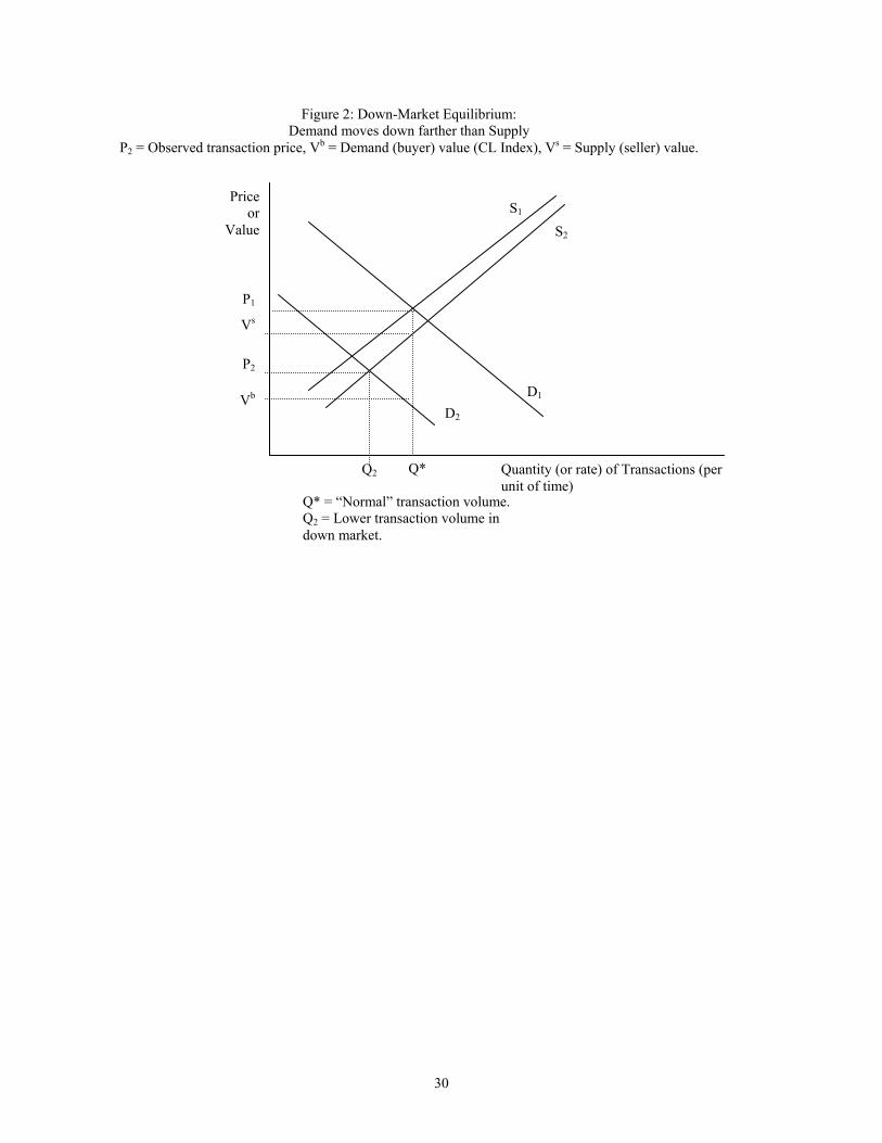
Figure 2: Down-Market Equilibrium: Demand moves down farther than Supply

P2 = Observed transaction price, Vb = Demand (buyer) value (CL Index), Vs = Supply (seller) value.

S2 S1

D2

Quantity (or rate) of Transactions (per unit of time)

Q*

Q* = “Normal” transaction volume. Q2 = Lower transaction volume in down market.

Q2

Price or

Value

D1

P1

Vs

P2

Vb

30

Figure 3: NCREIF Prices (shaded line) & Turnover Ratios (bars), 1984-2001:

NCREIF Prices & Turnover Ratios, 1984-2001

-0.5

-0.4

-0.3

-0.2

-0.1

0

0.1

0.2

84 85 86 87 88 89 90 91 92 93 94 95 96 97 98 99 00 01

Year

Log

Pric

e Le

vel

0%

5%

10%

15%

20%

Perc

ent P

rope

rties

Sol

d

31

Figure 4: Transaction-Based Value Indices of NCREIF vs Appraisal-Based NPI & Securities-Based NAREIT Indices Estimated Log Value Levels (Set AvgLevel=Same 84-01)…

Transaction-Based Value Indices of NCREIF vs Appraisal-Based NPI & Securities-Based NAREIT IndicesEstimated Log Value Levels (Set AvgLevel=Same 84-01)

-0.5

-0.4

-0.3

-0.2

-0.1

0

0.1

0.2

0.3

84 85 86 87 88 89 90 91 92 93 94 95 96 97 98 99 00 01

Transaction IndexSelection Corrected Variable LiquidityNCREIFConstant LiquidityNAREIT June 30

32

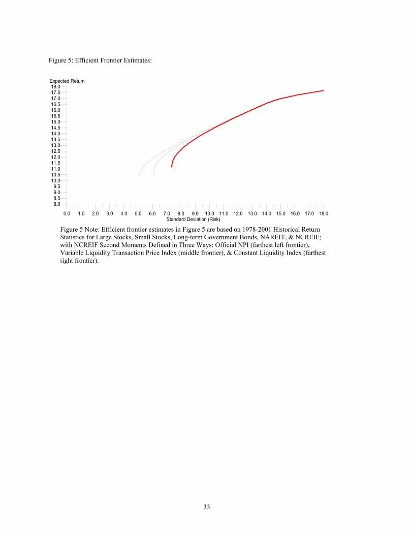
Figure 5: Efficient Frontier Estimates:

Standard Deviation (Risk)

Expected Return

0.0 18.01.0 2.0 3.0 4.0 5.0 6.0 7.0 8.0 9.0 10.0 11.0 12.0 13.0 14.0 15.0 16.0 17.0

8.0

18.0

8.59.09.5

10.010.511.011.512.012.513.013.514.014.515.015.516.016.517.017.5

Figure 5 Note: Efficient frontier estimates in Figure 5 are based on 1978-2001 Historical Return Statistics for Large Stocks, Small Stocks, Long-term Government Bonds, NAREIT, & NCREIF; with NCREIF Second Moments Defined in Three Ways: Official NPI (farthest left frontier), Variable Liquidity Transaction Price Index (middle frontier), & Constant Liquidity Index (farthest right frontier).

33

Table 1 Summary Statistics: Sold, Unsold Sample, and Acquisition Data

(by year) Year

Obs. (all obs.)

Obs. SOLD

Mean Price/SF SOLD

Mean SF (000s) SOLD

Obs. UNSOLD*

Mean SF (000s) UNSOLD

Properties Acquired

1983 769 35 43.83 108.3 734 131.2 1961984 996 73 45.19 89.7 923 175.1 2791985 1058 95 43.54 123.1 963 183.7 2991986 1084 96 53.04 114.4 988 190.8 3631987 1198 85 48.48 146.0 1113 197.7 3631988 1338 118 47.97 218.4 1220 211.4 4671989 1426 142 60.97 159.1 1284 222.7 4951990 1483 93 48.14 146.4 1390 228.6 4061991 1580 97 52.16 169.8 1483 234.9 2601992 1862 84 39.66 147.5 1778 229.7 1811993 1891 129 43.57 176.6 1762 261.4 2021994 1919 169 47.53 228.7 1750 273.4 3831995 1791 157 57.96 221.0 1634 291.1 5291996 2180 321 65.07 213.2 1859 284.1 6001997 2302 411 69.90 278.4 1891 296.8 5821998 2153 351 86.44 273.9 1802 294.2 6981999 2122 296 78.83 253.1 1826 311.0 7092000 2374 271 94.68 270.6 2103 317.2 6522001 1825 190 85.66 245.6 1635 332.6 433Total 31351 3213 28138 * Note: Unsold properties are all those in the database in the second quarter of each year. Data are available from 1982:2 to 2001:4.

34

Table 2: Results of Probit Model of Property Sale Probability, eqn.(10): Dep.Var: Sale Dummy

Explanatory Variable: Coef. Std. Err. t P>|t|95% Conf. Interval:

Jointven -0.10043 0.053277 -1.89 0.059 -0.20485 0.00399 Sqft -0.1192 0.050129 -2.38 0.017 -0.21745 -0.02095 Unleveraged -4.03E-07 4.19E-08 -9.61 0 -4.85E-07 -3.21E-07 yy_1984 dummy 0.243598 0.098751 2.47 0.014 0.050051 0.437145 yy_1985 dummy 0.357355 0.095719 3.73 0 0.169749 0.544961 yy_1986 dummy 0.352578 0.095472 3.69 0 0.165457 0.539698 yy_1987 dummy 0.237408 0.095987 2.47 0.013 0.049277 0.425539 yy_1988 dummy 0.364028 0.09257 3.93 0 0.182594 0.545463 yy_1989 dummy 0.430195 0.09105 4.72 0 0.25174 0.608651 yy_1990 dummy 0.181792 0.094127 1.93 0.053 -0.00269 0.366278 yy_1991 dummy 0.176392 0.093387 1.89 0.059 -0.00664 0.359427 yy_1992 dummy 0.023259 0.093818 0.25 0.804 -0.16062 0.207139 yy_1993 dummy 0.240322 0.090437 2.66 0.008 0.063069 0.417575 yy_1994 dummy 0.384063 0.088787 4.33 0 0.210045 0.558082 yy_1995 dummy 0.386426 0.089482 4.32 0 0.211045 0.561807 yy_1996 dummy 0.689181 0.085608 8.05 0 0.521392 0.85697 yy_1997 dummy 0.826553 0.084785 9.75 0 0.660378 0.992728 yy_1998 dummy 0.758925 0.085448 8.88 0 0.59145 0.926401 yy_1999 dummy 0.663404 0.08602 7.71 0 0.494808 0.832 yy_2000 dummy 0.547098 0.086068 6.36 0 0.378409 0.715788 yy_2001 dummy 0.495162 0.088578 5.59 0 0.321554 0.668771 Constant -1.52244 0.093628 -16.26 0 -1.70594 -1.33893

35

Table 3: Results of Selection-Corrected Hedonic Price Model, eqn.(11): Dep.Var.: Logsalepricepersf Explanatory Variable: Coef. Std. Err. t P>|t| 95% Conf.Interval Prop.Type Dummies: offcbd_dum 0.08638 0.036124 2.39 0.017 0.015578 0.157181offsub_dum 0.008358 0.021501 0.39 0.697 -0.03378 0.050499Regionalmall_dum 0.045721 0.048569 0.94 0.347 -0.04947 0.140914Warehouse_dum 0.015076 0.064085 0.24 0.814 -0.11053 0.14068industrial_dum 0.067487 0.066386 1.02 0.309 -0.06263 0.1976indflexspace_dum -0.20747 0.063151 -3.29 0.001 -0.33125 -0.0837Geog.Loc. Dummies : en_div dum 0.002651 0.031206 0.08 0.932 -0.05851 0.063814me_div dum 0.107814 0.032673 3.3 0.001 0.043776 0.171851se_div dum 0.036236 0.030905 1.17 0.241 -0.02434 0.096809sw_div dum -0.13883 0.031426 -4.42 0 -0.20042 -0.07724wn_div dum -0.03092 0.036955 -0.84 0.403 -0.10335 0.041514wp_div dum 0.194991 0.028543 6.83 0 0.139049 0.250934ne_div dum 0.133461 0.035192 3.79 0 0.064486 0.202437Hedonic Variables: Jointven 0.087378 0.021195 4.12 0 0.045836 0.128919Log Initial P/SF 0.670753 0.014861 45.13 0 0.641625 0.69988Time Dummies: yy_1984 -0.0364 0.088475 -0.41 0.681 -0.20981 0.137012yy_1985 0.008613 0.088112 0.1 0.922 -0.16408 0.181309yy_1986 0.007229 0.08786 0.08 0.934 -0.16497 0.179431yy_1987 -0.07893 0.086116 -0.92 0.359 -0.24771 0.089858yy_1988 -0.13781 0.085388 -1.61 0.107 -0.30517 0.029546yy_1989 -0.12772 0.086793 -1.47 0.141 -0.29784 0.042386yy_1990 -0.21525 0.084823 -2.54 0.011 -0.3815 -0.049yy_1991 -0.20536 0.083796 -2.45 0.014 -0.3696 -0.04112yy_1992 -0.31902 0.084091 -3.79 0 -0.48383 -0.1542yy_1993 -0.44499 0.082001 -5.43 0 -0.60571 -0.28427yy_1994 -0.29022 0.083115 -3.49 0 -0.45312 -0.12732yy_1995 -0.29898 0.083743 -3.57 0 -0.46312 -0.13485yy_1996 -0.25904 0.092656 -2.8 0.005 -0.44064 -0.07744yy_1997 -0.14885 0.098195 -1.52 0.13 -0.34131 0.043611yy_1998 -0.0325 0.0954 -0.34 0.733 -0.21948 0.154477yy_1999 -0.05973 0.09124 -0.65 0.513 -0.23856 0.119098yy_2000 0.039068 0.086277 0.45 0.651 -0.13003 0.208167yy_2001 0.052081 0.086077 0.61 0.545 -0.11663 0.220789Constant 1.867293 0.234462 7.96 0 1.407756 2.32683Lambda -0.26027 0.101305 -2.57 0.01 -0.45883 -0.06172-------------+ ------------ ----------- --------- --------- ------------- ---------- Rho -0.55363 Sigma 0.470126

36

Table 4: Estimated Annual Capital Returns to Institutional Commercial Real Estate, 1984-2001*

Yr UncorHed Heckman NPI Const-Liq** NAREIT84 1.76% -3.64% 7.58% -3.80%85 6.86% 4.50% 5.24% 9.85% 17.61%86 -0.33% -0.14% 2.66% -0.36% -1.67%87 -11.28% -8.62% 0.82% -14.03% -1.14%88 -3.58% -5.89% 0.89% 0.06% -11.31%89 2.87% 1.01% 0.92% 4.12% -6.77%90 -14.11% -8.75% -1.51% -20.43% -30.96%91 0.57% 0.99% -7.20% 0.73% 2.74%92 -14.64% -11.37% -10.72% -18.56% 3.53%93 -8.08% -12.60% -5.58% -2.39% 13.75%94 18.39% 15.48% 0.30% 22.23% -2.99%95 -0.88% -0.88% 2.82% -0.77% -1.88%96 10.53% 3.99% 3.74% 18.23% 8.26%97 13.58% 11.02% 6.40% 17.48% 24.88%98 10.32% 11.63% 9.94% 8.46% -9.42%99 -4.67% -2.72% 5.69% -7.21% -14.73%00 7.13% 9.88% 4.90% 4.41% 4.09%01 0.29% 1.30% 3.19% -1.14% 4.72%

* Index labels as follows: UncorHed = Uncorrected transaction-based hedonic price index based on equation (6), reflecting variable liquidity. Heckman = Selection-corrected (Heckman 2nd-stage) hedonic price index based on equation (11), reflecting variable liquidity. NPI = NCREIF Index appreciation returns (appraisal-based, equally-weighted across properties, including value of capital improvement expenditures, based on September 30 year end, make more contemporaneous with annual average transaction price based indices). Const-Liq = Constant Liquidity Value Index based on equation (15). NAREIT = NAREIT (National Association of Real Estate Investment Trusts) All REIT Price Index capital return (based on year ending June 30, in order to make more contemporaneous with annual average transaction price based indices). ** Note that it is not possible to estimate a constant-liquidity adjustment ( tγ̂ ) in the base year omitted in the model (1983), hence, the constant liquidity index return cannot be computed in the first year (1984 for returns).

37

Table 5: Return Statistics (continuously compounded annual capital returns), 1984-2001: Transaction

Index Selection Corrected

NCREIF Constant Liquidity

NAREIT

Mean 0.76% 0.52% 1.32% 1.22% -0.08% Std.Dev 9.61% 8.33% 5.22% 12.07% 12.99% AutoCorr 8.08% 6.56% 80.06% 8.83% 10.16% Cross Correlation: Transaction Index 1 95.08% 58.39% 96.57% 40.32% Selection Corrected 1 63.07% 83.85% 25.97% NCREIF 1 49.52% 2.43% Constant Liquidity 1 50.17% NAREIT 1 Cycle Amplitude & Turning Points: Fall: Period (yy – yy): 85-93 85-93 89-93 85-93 85-90 Magnitude 48.58% 45.36% 25.02% 50.86% 51.84% Rise: Period (yy – yy): 93-01 93-01 93-01 93-98 90-97 Magnitude 54.69% 49.71% 36.98% 65.63% 48.29%

38

Table 6: Allocations Within 5-Asset Class Maximum Sharpe Ratio Portfolio*:

on:

Official NCREIFVa

Transactions 1 2 3

1 2 3 1 1 18

52.33% 32.56% 9.27%ased on 1978-2001 historical total returns statistics (30-day T-Bill return as riskfree interest te), except as noted for private real estate second moments.

Private real estate second moment inputs based riable Liquidity

Asset Class:

Index IndexConstant Liquidity

IndexLarge Stock 2.09% 6.47% 6.68%Small Stocks 9.10% 5.46% 5.65%Long-term Bonds 6.46% 5.50% .40%REITs 0.00% 0.00% 0.00%Private Real Estate *Bra

39

40

Endnotes

1 Further developments in these procedures in the real estate economics literature have

included Bryan and Colwell (1982), Case and Shiller (1987), Shiller (1991), Clapp and Giacotto

(1992), and Goetzmann (1992). A related approach is the use of “appraised values” or

“assessed valuations” derived from asset valuation professionals. 2 Gompers and Lerner (2000) employ the Heckman correction procedure in a study of the

venture capital market. 3 See, for example, Fisher, Geltner and Webb (1994), and Fisher and Geltner (2000). However,

these procedures do not explicitly or separately identify and control for the effect of variable

liquidity on market value changes. 4 Note also that the seller distribution represents the entire physical stock of the asset in

question. Sellers who are “not in the market” can be characterized as having very high

reservation prices. 5 Allowing for downward-sloping asset demand and upward-sloping asset supply is consistent

with traditional assumptions in the real estate literature. There is also growing acceptance of

such an assumption in the financial economics literature, notably concerning private equity

markets (e.g., see Gompers and Lerner (2000) regarding the venture capital industry), and even

concerning public securities markets (Shleifer 1986). 6 Not all buyers and sellers in the overlap region will transact within any given period of time.

Rather, all buyers and sellers with reservation prices in this region have a possibility of

achieving a match. The overlap region is not a distribution of the expected transaction prices. In

some pairings within the overlap region these two parties’ reservation prices will be very close

and there won’t be much room for negotiation, while in other pairings the two reservation prices

could be quite far apart (i.e., a buyer from far up to the right end of the overlap region deals with

a seller from far down to the left end of the overlap region). 7 The classical model of search represents potential trading partners looking for each other as a

Poisson arrival process. Consider a representative seller whose reservation price is x. Potential

buyers arrive according to a Poisson process with arrival rate λ, and these buyers are drawn

randomly from the buyer frequency distribution. Hence, the probability that any one buyer will be

a compatible partner equals the proportion of the buyer frequency distribution to the right of x.

Label this proportion G(x). Then the sale of this seller’s property (which must be at a price of at

least x) is governed by a Poisson process with arrival rate λG(x). The expected time-on-the-

41

market (“TOM”) for this property in the current market is the inverse of this arrival rate: E[TOM] =

1 / (λG(x)). Clearly, the farther to the right is the buyer frequency distribution (i.e., the greater

the overlap of buyers and sellers), the greater will be G(x), and the shorter will be the expected

TOM (i.e., greater “liquidity” in the market). 8 There are alternative models that could explain pro-cyclical variable liquidity. For example, pro-

cyclical variable liquidity could result from the reservation price distributions retaining their mean

values but spreading out to increase liquidity (due to the increased overlap) and shrinking to

decrease liquidity. This would imply that buyers and/or sellers become less certain about what

the market value is during “up” markets, and more certain during “down” markets, a pattern that

seems implausible. In the real world, bad news seems to engender more uncertainty among

market participants than good news. Another alternative is to have buyer and seller distributions

move equally along the horizontal axis in terms of their mean values, but to have the total

number of buyers increase and decrease in a pro-cyclical manner. In effect, buyers “come out of

the woodwork” during the up market, and retreat out of the picture during the down market. But

this model is effectively the same as the one we are depicting. 9 Formally, one can also define a constant-liquidity index relative to the sellers’ distribution of

prices, where the buyers’ distribution would move in lock-step following the sellers’ lead (just the

opposite to the definition we are pursuing in this paper). (This would correspond to point VS in

Figure 2.) While such an index might be of interest for purposes of tracing out movements on

the supply side of the market, it would not trace out price changes that would enable asset

owners to realistically maintain a constant time-on-the-market across the market cycle. Asset

owners must sell to buyers, hence, it is the buyers who determine the prices that are required to

maintain a constant “ease of selling” (or constant expected time-on-the-market for sellers). 10 The other difference between Figure 1 and Figure 2 is that we have transposed the axes (in

conformity with classical supply and demand diagrams), such that the horizontal axis in Figure 2

is the volume axis, and the vertical axis in Figure 2 is the price or value axis. Thus, movements

down along the vertical axis in Figure 2 correspond to movements to the left along the horizontal

axis in Figure 1. When the market moves “down” (e.g., in response to bad news), both demand

and supply functions move down along the vertical (value) axis, but demand moves farther

under pro-cyclical variable transaction volume. 11 Our assumption of trades at the midpoint is more realistic than the assumption used in many

previous studies in the real estate literature that all trades are at the buyer’s offer price. It is

also consistent with Wheaton’s (1990) assumption in his search model of the housing market.

42

PijtX

bi

12 This model is frequently applied to labor supply, where a market wage is observed only if the

market wage offer exceeds a person’s reservation wage. Such a model is very similar to our

model (there are buyer and seller distributions and observability is determined by an equation

such as (4)), except we have a different assumption about the observed transaction price (our

midpoint price assumption) and we focus on intertemporal changes. Nevertheless, the nature of

the censoring mechanism is identical. A good discussion of this model, applied to the labor

market example, is presented in section 8.4 of Maddala (1985). 13 Recall that Zt is a zero/one time-dummy variable, so the change in the market value between

period t-1 and period t simply equals the difference between the two time-dummy coefficients. 14 For example, in a typical real estate application one of the variables would typically be

property age. To index the market value change over time of a representative property, the

effect of the property’s aging must be included. On the other hand, an index of the overall

property market value changes would not include the age variable. 15 Other potentially interesting applications are suggested by this model. For example, as the

variance in the dispersion terms ( tεsi and tε ) govern the slopes of the demand and supply

schedules in Figure 2, it may be possible to gain insight regarding demand and supply price

elasticity based on the model described here. (See the Appendix for more detail.)

16 The NPI is a quarterly index of U.S. institutionally-held commercial investment real estate total

returns (broken out by “income” and “appreciation” components), commencing in 1977, and

produced by the National Council of Real Estate Investment Fiduciaries (see www.ncreif.org).

As of 2001 the index tracked the performance of about 3,300 properties with an aggregate

market value in excess of $100 billion, and it is widely used as both an investment performance

benchmark and a general investment research tool for the asset class. 17 Both empirical evidence and optimal appraisal theory support this claim. Regarding appraisal

theory, see most notably: Quan and Quigley (1989, 1991), Geltner (1997), Childs, Ott, and

Riddiough (2002a, 2002b), and Fisher and Ong (2002). For empirical evidence of appraisal lag

see recent articles by Diaz and Wolverton (1998), Fisher and Geltner (2000), and Clayton,

Geltner and Hamilton (2001). 18 The NPI database is proprietary and access limited. Direct access to individual property level

data was limited to only one of the authors of this study, Jeff Fisher, NCREIF Consulting

Director of Research and Technology. 19 Properties located in the East and West tend to be of higher values than those located in the

43

South; hence, the value of the properties located in the East, Midwest, West, and South

represent approximately 27, 16, 36, and 21 percent of the aggregate value of the database,

respectively 20 Individual office and retail properties are generally higher in value than the industrial and

apartment properties. Office properties represent approximately 42% of the aggregate value of

the database, while the industrial, retail, and apartment property classes represent 18 to 20%

each. 21 Individual property characteristics (e.g., square footage) are not available prior to 1982:2;

thus, the study period is restricted to begin in 1983. 22 The number of sold properties is less than the difference between the number of properties

that have ever been in the index and the number currently remaining in the index because some

properties exit the index by other means than sales (e.g., the NCREIF member owning the

property quits NCREIF). The number of observations exceeds the number of properties in the

database because most properties are held more than one year, and we obtain annual

observations of the variable values for each property. 23 The price index depicted in Figure 3 is a selection-corrected transaction-price-based index of

the type described in equation (11) (not the appraisal-based official NPI). 24 The property-type dummies include: CBD office, Suburban office, regional shopping mall,

warehouse, industrial research and development facility, and industrial flex space facility. The

geographical location dummy variables include all but one of the eight NCREIF multi-state

regional divisions of the U.S.: Northeast, Mideast (similar to the census Middle Atlantic region),

Southeast, Southwest, East North Central, West North Central, Mountain, and Pacific.

(Mountain was the omitted region in the specification, so the regional coefficients represent

incremental differences relative to that region.) 25 For example, the property purchase price will tend to reflect the value effect of such property

characteristics as size, age, physical and location quality, income earning potential, risk, and so

forth. 26 Successful consummation of a sale transaction for a joint venture property requires a price

that satisfies at least two different owners. This may introduce a greater degree of difficulty

agreeing to a sale, hence requiring a higher price to induce the sale. An alternative hypothesis

would suggest that joint venture ownership may tend to involve agency costs due to possible

conflicts of interest between the two owners. Such agency costs could drive down the

investment value of the property to the joint venture owners, leading them to sell at a lower

44

price. The sign of the coefficient on the jointven variable in the price equation should reflect the

balance of these two possible effects. 27 The official NCREIF Index reports quarterly appreciation returns from which a cumulative

value level index can be developed. However, we have modified the official NCREIF Index in

two respects to make it more comparable to the transaction indices we have developed. First,

we are using an equal-weighted version of the NCREIF Index rather than the value-weighting in

the official index. Second, we have added back in the capital improvement expenditures that the

official NPI subtracts from the end-of-period appraised value to compute the appreciation return.

We want our version of the NCREIF appreciation index to incorporate the value-enhancing

effects of capital improvement expenditures, as reflected in the actual appraisals of the

properties, because the prices on which our transaction-based indices are based certainly

reflect the (market) value of the capital improvements (as perceived by the buyers and sellers).

The result of this second change is that our NCREIF Index rises a little faster and farther over

time than the official NCREIF appreciation index. In addition, we are using NCREIF appreciation

index value levels as of the third quarter each year, for greater comparability with the

transaction-based indices that represent annual average value levels, aggregated across the

entire calendar year. (As the official NCREIF Index includes properties that are not reappraised

every quarter, the third quarter index likely reflects average appraised values as of a quarter or

more previous, more likely around the middle of the calendar year.) 28 This is the "All REIT" share price index produced by the National Association of Real Estate

Investment Trusts (www.NAREIT.org). We are using the NAREIT Index level as of June 30

each year, to make it more compatible with the transaction-based indices that reflect the

average sale price during the calendar year (the same reason that we used the September

NCREIF Index). This is an admittedly “first approximation” type approach for correcting the

asynchronous problem. A more precise approach would be the fractional time-dummy

specification of Bryan & Colwell (1982). However, this approach would likely add estimation

noise to the hedonic regression. 29 The types of properties held by REITs are not exactly identical to the types of properties

represented in the NCREIF database. In addition, REIT management policies and

considerations (including property trading, development projects, and financial strategy) add a

layer of investment performance results on top of that of the underlying “bricks and mortar”

represented by operating property assets in place. 30 See Ling and Ryngaert (1997), and Ling and Naranjo (1999).

45

31 Both REIT equity and CMBS debt markets retrenched particularly in the latter half of 1998

and early 1999. Recall that our transaction-based indices reflect average asset prices

aggregated across the calendar years. Thus, the annual return indicated for 1999 more closely

reflects differences between mid-1999 and mid-1998 (rather than end-of-year based returns). 32 Lower quality properties would tend to suffer the worst performance hit during a severe real

estate slump. Conservative institutional investors such as the pension funds whose capital is

managed by NCREIF members may prefer to unload under-performing real estate during such

a period, even though such a disposition policy makes their investment performance look worse

during the down market. They may then try to recoup the performance hit by selling star

properties in the upswing. The overall average growth in the selection-corrected index across

the entire cycle is very similar to the uncorrected hedonic index that directly reflects observed

sales, a result consistent with such behavior. 33 Data on historical total returns for all five asset classes was obtained from Ibbotson

Associates. The indices used to represent the five asset classes were: For the large stock, small

stock, and long-term Government bonds asset classes the indices taken from the Ibbotson

Stocks, Bonds, Bills & Inflation Yearbook; For the real estate asset classes, the NAREIT All

REIT Index, and the NCREIF Property Index. 34 These two alternative assumptions for the private real estate second moments had to be

based on the capital returns only, during the 1985-2001 period available in the transaction price

indices that we were able to estimate based on transaction price data availability as described

previously. However, periodic returns series second moments are usually determined almost

entirely by the capital returns component of the total returns, and as noted, the 1985-2001

period includes a complete cycle in the private real estate market. Therefore, these limitations in

our data may be less problematical than might be supposed. It should also be noted that

hedonic price models similar to the one used in Equation (11) could be employed to estimate a

total return index for a population of properties such as the NCREIF database, via the procedure

known as “mass appraisal”. The hedonic model would be employed to estimate the current

value of each property in the index as of each period of time, and these disaggregate value

estimates would then be combined with property-level periodic income data to derive the total

return for each property, each period. The disaggregate total returns would then be aggregated

up to the index level. 35 The correlation of the constant-liquidity index during 1985-2001 was 11% with the large stock

index, 29% with the small-stock index, and -2% with the long-term bond index. The correlation

46

of the official NCREIF Index with these other asset classes during the complete 1978-2001

period was 10%, 5%, and -23% respectively. The variable liquidity index correlations were in

between these two extremes: at 10%, 19%, and -7%. 36 One plausible way to interpret the implications of the two alternative transaction-based real

estate indices from an investment policy perspective is as follows. The variable liquidity index

represents the periodic returns that private real estate investors actually achieved based on the

sales volume that actually occurred, which reflected the trade-off that asset owners made

between the transaction prices they chose to agree to and the average time-on-the-market and

sales volume they chose to accept. As this price index reflects sharply lower liquidity during

down markets, the risk statistics implied by such a variable liquidity index might be deemed

appropriate for an investor who is willing to “pre-commit” to largely avoid selling private real

estate assets during down periods in the real estate market (i.e., the investor is willing to

sacrifice liquidity during those periods). On the other hand, the constant liquidity index reflects

the risk that would face an investor who wants to be able to sell private real estate in as great a

volume and/or with as low an expected time-on-the-market when the real estate market is down

as when it is up. Thus, if the investor is not willing to “pre-commit” to sacrificing liquidity during

real estate down markets (which historically have sometimes lasted for prolonged periods of

time), then the risk statistics implied by the constant-liquidity index may be more appropriate for

such an investor’s decision making. As such “pre-commitments” regarding liquidity requirements

are not generally assumed necessary in standard portfolio allocation analyses that are based on

publicly-traded asset classes, the default “apples-vs-apples” private real estate risk statistics to

employ in such analyses might arguably be considered to be those derived from the constant-

liquidity index. 37 The Sharpe Ratio is the portfolio mean return in excess of the riskfree interest rate (T-Bill

return in this case), divided by the volatility of the portfolio. The maximum Sharpe Ratio portfolio

is the risky asset combination that would theoretically be preferred by investors of any degree of

risk aversion or risk tolerance, based on the given risk and return expectations, assuming that

long and short positions in the riskless asset are possible (and that the “riskless” asset is truly

riskless from the investors’ perspective). 38 The REIT asset class does not appear in the Sharpe maximizing portfolio under any of the

private real estate risk assumptions, largely because during the particular historical period

examined here (1978-2001) the REIT Index was nearly dominated by the Small Stock Index.

REITs and small stocks had 63% positive correlation, but small stocks had substantially higher

47

average return (18% versus 13%) and not much more volatility (18% versus 16%). It should be

noted that this result is sensitive to both the historical time period examined, and to the definition

of the REIT index (e.g., all REITs versus only equity REITs).