“Liquidity requirements, liquidity choice and financial stability”*

Douglas W. Diamond

Anil K Kashyap

University of Chicago Booth School of Business and National Bureau of Economic Research

December 2015

Abstract

We study a modification of the Diamond and Dybvig (1983) model in which the bank may hold a liquid asset, some depositors see sunspots that could lead them to run, and all depositors have incomplete information about the bank’s ability to survive a run. The incomplete information means that the bank is not automatically incentivized to always hold enough liquid assets to survive runs. Regulation similar to the liquidity coverage ratio and the net stable funding ratio (that are soon be implemented) can change the bank’s incentives so that runs are less likely. Optimal regulation would not mimic these rules.

* Prepared for the Handbook of Macroeconomics. We thank Franklin Allen, Gary Gorton, Guido Lorenzoni, Annette Vissing-Jorgenson, Nancy Stokey, Nao Sudo, John Taylor, Harald Uhlig and seminar participants at the Asian Development Bank Institute, East Asian Economic Seminar, Imperial College, Melbourne Institute Macroeconomic Policy Meetings, National Bureau of Economic Research Monetary Economics meeting, the Bank of England, European Central Bank, Centre for Economic Policy Research and Centre for Macroeconomics Conference on Credit Dynamics and the Macroeconomy, Riksbank, and the University of Chicago for helpful comments and Adam Jorring for expert research assistance. We thank the Initiative on Global Markets at Chicago Booth, the Fama Miller Center at Chicago Booth and the National Science Foundation for grants administered through the NBER for research support. All errors are solely our responsibility.

1

Introduction

In September 2009 the leaders of 20 major economies created the Financial Stability Board (FSB) whose purpose is to “coordinate at the international level the work of national financial authorities and international standard setting bodies (SSBs) in order to develop and promote the implementation of effective regulatory, supervisory and other financial sector policies.” Since that time the financial system has undergone a regulatory overhaul.

The term “macroprudential” regulation has become synonymous with much of this effort. As we explain in the next section, what that means in practice remains somewhat elusive. But, there are two tangible changes that are on track to occur over the remainder of this decade. One widely studied set of reforms pertain to the rules regarding capital requirements for banks. Less well- understood is that, through their cooperation via the Basel Committee on Bank Supervision, the major economies have also agreed also to implement by 2019 new rules governing banks’ debt structures and requirements to hold certain types of liquid assets.

To date there is a remarkable asymmetry in the economic analysis of the capital and liquidity regulations. The pioneering work of Modigliani and Miller (1958) provides a solid theoretical framework for analyzing capital regulation. Any student taking a first course in corporate finance will encounter this theory and there is a massive empirical literature that explores the theory’s predictions. Capital regulations for banks at the international level go back to 1988 and there many empirical examinations of the impact of these regulations.

In contrast, there is no benchmark theory regarding liquidity provision by intermediaries. Indeed, financial economists even have competing concepts that they have in mind when discussing liquidity, so that there is no generally accepted empirical measure of liquidity economists study. Allen (2014), in his survey of the nascent literature on liquidity regulation, concludes by writing “much more research is required in this area. With capital regulation there is a huge literature but little agreement on the optimal level of requirements. With liquidity regulation, we do not even know what to argue about.”

Nonetheless, the global regulatory community has agreed on certain liquidity requirements (Basel Committee on Bank Supervision (2013a, 2014)). Two new concepts, the liquidity coverage ratio and the net stable funding ratio, have been proposed and banks by 2019 will be compelled to meet requirements for these ratios. Thus, it seems fair to say we are in a situation where practice is ahead of both theory and measurement.

In this paper we survey the existing work on liquidity regulation and develop a framework for discussing the regulation. The theory that we propose suggests, in certain parameterizations, regulations bearing some resemblance to the liquidity coverage ratio and net stable funding ratio can emerge as ones which will improve outcomes relative to an unregulated benchmark. However, the regulations that arise in our model would naturally differ across banks, depending

2

on certain bank characteristics, so they do not mimic exactly the ones that are on track to be implemented.

The critical ingredients in our model are the following. First, we consider banks which are spatially separated and hence do not compete aggressively for deposits. Treating the bank as monopolist simplifies the analysis by allowing us to side-step some complications that arise from having to model the deposit market equilibrium. The model can also be interpreted as a description of the aggregate banking system, which for many financial stability and regulatory discussions is the object of primary concern and under this interpretation ignoring the deposit competition is perhaps more natural.

Second, we assume that intermediaries provide liquidity insurance for customers who have uncertain withdrawal needs (or consumption desires). We build on the Diamond and Dybvig (1983), henceforth DD, model of banking in which banks provide this insurance by relying on the law of large numbers to eliminate idiosyncratic customer liquidity needs.

For those familiar with DD, we make two modifications. The first is allowing the bank to invest in a liquid asset that has a rate of return exceeding the return from liquidating illiquid assets and thus is the efficient way to arrange to pay customers that need liquidity. This introduces a tradeoff between lending and holding liquidity as in Bhattacharya and Gale (1987) and several papers of Allen and Gale (1997 and others).

The other modification to DD is the form of run risk that the banks face. Banks are assumed to have a good assessment of the aggregate needs of their customers for fundamental reasons. But, they also know that some customers will receive a signal about the bank which could lead to a run. The sunspots that we consider are a metaphor for people being concerned with the health of the bank, but not having a fully formed set of beliefs about the bank’s solvency status. In making their decisions we assume that customers are unable to fully evaluate the ability of the bank to honor deposits. Given the complexity of modern banks it seems realistic to presume that most customers cannot precisely determine their bank’s maturity mismatch and hence its vulnerability to a run. The imperfect information creates a challenge for the banks because their customers will not necessarily know if the bank is prudently holding liquidity or not, which reduces the incentive to hold liquidity.

In the event that a run does occur, we depart from DD and Ennis and Keister (2006) to allow for the possibility that not all customers seek to withdraw their funds. We believe it is useful to analyze partial runs for two separate reasons. One is that in practice there do seem to be some sticky deposits that do not flee even in times of considerable banking stress. In addition, even before troubles occur it is usually clear which types of deposits are prone to running. So this allows us to talk about policies for different types of withdrawal risk.

Within this environment we can assess the vulnerability of the financial system to runs under different regulatory arrangements. In the baseline case, we assume that banks simply maximize

3

their profits and see which types of equilibria arise. As usual in DD style models, the outcomes depend critically on how depositors form beliefs. It is possible, under certain parameter configurations, that the pure self-interest motives of the banks will sufficient to insure that the system will be run proof even if depositors had no detailed information about a bank’s liquidity holdings. In these situations, added liquidity could not influence whether a given depositor would choose to join a run if one was feared.

We describe several reasons why depositors may not be able to use some types of disclosure of a bank’s liquidity holdings to determine if the holding is sufficient to allow it to survive a run. To fix ideas, one can consider whether a bank would choose to hold this sufficient amount of liquidity even if its choice between liquid assets and illiquid loans was completely unobservable. In circumstances where depositors cannot be sure about how changes in liquidity holdings impact the robustness of banks to runs, the banks will typically face a tension in deciding how much to fortify themselves against the risk of a run. They can always choose to be sufficiently conservative to be able to withstand a worst case of fundamental withdrawals as well as a panic. But in order to do that, they will engage in very little lending, and the forgone profits from deterring the run will be high. The additional liquidity to survive a run will turn out to be excessive whenever a run is avoided. Hence, it is possible they will make more profits from added lending which would leave them unable to always be able to sustain a run.

We next allow regulatory interventions that place restrictions on present and possibly on future bank portfolio choices. In the baseline set up, the banks have perfectly aligned incentives to prepare to service fundamental aggregate withdrawal needs. So the regulatory challenge is to determine whether a requirement that distorts their private incentives towards being more robust to a run will improve outcomes. We allow for regulation that is inspired by the two impending Basel rules.

One variant requires an initial liquidity position that must be established before depositors make their intentions clear. This can function like the “net stable funding ratio” that is proposed as part of the Basel reforms. A second option is a mandate to always hold additional liquid assets beyond those needed for the fundamental withdrawals. This imposes both present and future minimum holdings of liquid assets. This regulation looks like a traditional reserve requirement for the bank, but can also be interpreted as a kind of “liquidity coverage” ratio that is part of the Basel reforms.

One point of contention regarding the liquidity coverage ratio that has emerged is whether required liquidity can be deployed in the case of a crisis. Goodhart (2008) framed the issue nicely with a now famous analogy of “the weary traveller who arrives at the railway station late at night, and, to his delight, sees a taxi there who could take him to his distant destination. He hails the taxi, but the taxi driver replies that he cannot take him, since local bylaws require that there must always be one taxi standing ready at the station.”

4

One way to interpret the Goodhart conundrum is to recognize that, broadly speaking, there are two ways to think about the purpose behind liquidity regulations. One motivation can be to make sure that banks can better withstand a surge in withdrawals should one occur. From this perspective mandating that the last cab cannot depart the station seems foolish. Another possible motivation is to design regulations aimed at reducing the likelihood of a withdrawal surge in the first place. Our model helps highlight the potential incentive properties of regulation and can potentially explain why mandating the presence of some unused liquidity could be beneficial.

In studying how private and social incentives for liquidity choices diverge, our main conclusion from analyzing the two Basel-style regulations is that they may improve outcomes relative to the ones that arise from pure self-interest, but each brings potential inefficiencies. Hence, we briefly also describe the solution of the mechanism design problem for a social planner who has less information about withdrawal risk than the bank does and seeks to optimally regulate banks to avoid runs. That solution provides a natural benchmark against which to judge the Basel-style regulations.

The remainder of the paper is divided into five parts. Section two contains our selective overview of previous work. We organize this into three sub-sections. We begin with an overview of the emerging policy proposals and research regarding macroprudential regulation. We then hone in on the enormous and rapidly growing literature on capital regulation. We provide our perspective on how to group these papers and highlight several recent excellent surveys on the pure effects of capital regulation. We close with a review of the most relevant papers for our questions that motivate us about liquidity regulation.

Section three introduces the benchmark model. We explain how it works under complete information. We also derive a generic proposition that holds with incomplete information that describes when the bank’s preferred liquidity choice will be sufficient to deter a run. Generically, however, privately chosen levels of liquidity need not be sufficient to deter runs. So this opens the door for regulations that might do so.

In section four we analyze the two types of liquidity regulation that are akin to the ones contemplated under the Basel process. We first demonstrate that a particular type of regulation that requires the bank to hold liquid assets equal to a fixed percentage of deposits at all times can potentially deter runs. This works because the liquidity mandate, combined the bank’s self-interest to prepare to service predictable deposit outflows, leads the bank to hold more overall liquidity than it would otherwise. Because depositors understand this, it removes the incentive to run in some cases. We also consider alternative assumptions about depositors’ knowledge and the information available to regulators and assess the vulnerability of the bank to runs in these scenarios.

In section 5, we describe a couple of extensions of the baseline model. The first sketches a mechanism design problem where the regulator does not have all of the bank’s information and

5

seeks to implement run-free banking. We fully characterize the solution to this problem in Diamond and Kashyap (2016), here we describe the main findings from this exercise. It turns out that a regulator with sufficient tools can induce the bank to hold the proper amount of liquidity despite the private information advantage possessed by the bank.

We also briefly discuss capital regulation. We explain why as a tool for managing liquidity problems, capital requirements can be relatively inefficient compared to the other regulations that we have reviewed. Obviously in a richer model where both credit risk and liquidity risk are present, capital and liquidity regulations can serve different purposes. We describe some of these differences.

Section six presents our conclusions. Besides summarizing our findings, we also pose a few open questions that are natural next steps to consider in addressing the issues analyzed in this paper.

2. Literature Review

Research on financial regulation has exploded since the global financial crisis, and the number of regulatory interventions and tools has also expanded massively. To review all of this work would require a book. To keep our review manageable, we limit our discussion to focusing on the theoretical underpinnings and rationale behind these changes.1

2.1 Macroprudential regulation

Clement (2010) provides the interesting history of the origins and evolution in the meaning of the phrase “macroprudential.” His best estimate is that the term appeared first in 1979 in the documents of the committee that was the fore-runner to the Basel Committee on Bank Supervision. The first public document using the term which he can identify was a report by the committee now known as the Committee on the Global Financial System. It defined macrorpudential policy as promoting “the safety and soundness of the broad financial system and payments mechanism.”

The phrase took on added prominence when it was the focus of a September 2000 speech by Andrew Crockett (who was then the General Manager of the Bank for International Settlements (Crockett (2000)). He defined the objective of macroprudential policy to be “limiting the costs to the economy from financial distress, including those that arise from any moral hazard induced by the policies pursued.” Crockett’s rational for calling for macroprudential policies was his belief that optimal choices for a single institution could create problems for the financial system 1 For a diverse set of perspectives on the changing post-crisis regulatory landscape see Čihák, Demirgüç-Kunt, Martínez-Pería and Mohseni-Cheraghlou (2013), Financial Stability Board (2015), Claessens and Kodres (2014), Basel Committee on Bank Supervision (2013), and Fisher (2015).

6

as a whole. He was explicitly focused on the distinction between the supervisory challenges for monitoring an individual institution and those for protecting the aggregate financial system.

Crockett did not offer precise microeconomic foundations for why the private actions of individual actors would not be aligned with social welfare, but he did give a few examples where he saw the potential for divergence. One possibility he cited is that one bank seeking to limit its credit exposures could choose to cut lending to its clients, but if all banks did this a credit crunch could ensue that would trigger a recession. A second example was the possibility of what we would now dub to be a fire-sale where all agents simultaneously cut back on asset exposures due to falling prices and in the course of doing so exacerbate the price decline. A third problem arises if many lenders shorten the maturity of their funding to a particular borrower, then the risk of a run can increase so that they are all more vulnerable.

Our view is that Crockett’s spotlight on the divergence between the narrow private interests of individual institutions (or supervisors monitoring a single institution) and the interests of overall society is exactly the right focus for considering macroprudential policies. Indeed, this literature would be well-served to move in the direction where all macropurudential papers start by clarifying why (and when) social and private interests diverge. The challenge for both for researchers and policymakers is the difficulty in formalizing and prioritizing the exact reasons for the divergence. To clearly see the problem, compare three prominent perspectives on macroprudential regulation that have followed Crockett.

First, various BIS documents (e.g. Clement (2010)) now interpret Crockett as having identified two types of problems that are to be addressed. One relates to the build-up of risks over time, that are often now referred to as the pro-cyclicality of the financial system or the “time dimension” of the macroprudential policy problem. The other relates to the distribution of risks within the financial system, the so-called “cross-sectional dimension” of the problem. Many official sector documents adopt the convention of separating time-series and cross-sectional macrorprudential problems. As Clement (2010) notes, while the BIS work in this area has been relatively precise in the way these issues are discussed, “the usage of the term in the public sphere has on occasion been loose. It is not uncommon for it to be employed almost interchangeably with policies designed to address systemic risk or concerns that lie at the intersection between the macroeconomy and financial stability, regardless of the specific tools used.”

In contrast, Hanson, Kashyap and Stein (2011) start with a particular view of “how modern financial crises unfold, and why both an unregulated financial system, as well as one based on capital rules that only apply to traditional banks, is likely to be fragile.” Their perspective, appealing to the model in Stein (2012), presumes that banks will find it cheaper to fund themselves with short term debt than equity, so that banks have limited incentives to build strong equity buffers in normal times. If, in a crisis, such banks suffer substantial losses, then the market value of debt claims can fall below the face value, which will deter them from raising

7

new equity (Myers (1977)). Consequently, in this case the banks are likely to comply with capital regulations by shrinking their asset base. Hence, Hanson et al argue that the goal of macroprudential regulation should be to “control the social costs associated with excessive balance-sheet shrinkage on the part of multiple financial institutions hit with a common shock.”

A recent survey by the Norges bank staff, Borchgrevink, Ellingsrud and Hansen (2014), argues that in fact there are six market failures that can give rise to macroprudential concerns. These are pecuniary externalities, interconnectedness externalities, strategic complementarities, aggregate demand externalities, market for lemons and deviations from full rationality. Not surprisingly they conclude “Because of the diversity of these categories, policy lessons diverge. There is yet no “workhorse"model for policy analysis.” Though they do argue that capital and liquidity regulation should tuned to aggregate conditions, not just those of individual banks, and that borrowers should be subjected to time-varying policies that aim to force them to internalize the costs of excessive borrowing.2

We share the Borchgrevink et al (2014) conclusion that the macroprudential literature at this point remains in sufficient flux that it is too soon to reach firm conclusions about where it will lead. Hence, for the remainder of our analysis we focus on capital and liquidity regulation where the range of issues to be considered can be narrowed and where specific global policies are being implemented.

2.2 Capital regulation

For an overview of the literature on capital regulation, it is useful to sort papers along two dimensions. The first regards what is assumed regarding the Modigliani-Miller (1958) (henceforth MM) capital structure propositions. As in all models of corporate finance, absent failures of one of the MM propositions any choices regarding capital structure will be inconsequential. There have been four primary MM violations that have drawn attention in the literature.

One concerns that existence of deposit insurance. If certain parts of a bank’s capital structure is protected from losses by the government, that can create risk-shifting incentives for equity holders. In many models, bank managers working on behalf of the equity owners face an incentive to gamble after adverse shocks that goes unchecked because depositors are immune from losses that they would suffer if the gamble fails.

2 Others have also chosen to organize their analyses around distinctions between the kinds of tools that can be deployed. For example, Aikman, Haldane, and Kapadia (2013) classify tools into three groups: those that operate on financial institutions’ balance sheets; those that affect the terms and conditions on financial transactions; and those that influence market structures. While Cerutti, Claessens, and Laeven (2015) present empirical analyses comparing 12 types of different regulations.

8

A second distortion is concerns over guarantees to protect equity holders of banks from losses. Usually this is couched as a problem of having some banks that are assumed to be “too big” or “too-interconnected” to fail. But, in the recent global financial crisis, there were also cases in some countries where equity owners of smaller, non-systemic banks were insulated from losses due to political connections.

A third violation regards the MM assumption of complete financial markets. With incomplete markets, an institution that creates new securities could be valuable. In the banking context, deposits are a leading example of special security that banks might create.

Finally, there are many models where either asymmetric information or moral hazard problems are considered. Some of the prominent examples include the possibility that borrowers know more about their investment opportunities than lenders, or that borrowers can shift the riskiness of their investments after receiving funding.

So unlike much of the research on non-financial corporations, the trade-off theory of capital structure, whereby firms prefer debt for its tax advantages and balance those benefits against costs of financial distress, has not figured prominently in the banking research on capital regulation. Rather, regulation is usually justified on the grounds of addressing one of these other four problems. The type of regulation that can be welfare improving will differ depending on which of these other frictions is assumed to be present.

The second important dimension one which the literature can be organized concerns the economic services that banks are assumed to provide.3 Broadly, there are three types of services that have been modeled. The first presumes that certain financial institutions can expand the amount of credit that borrowers can obtain (say, relative to direct lending by individual savers). The micro-founded theories typically assume that borrowers can potentially default on loans and so any lender has to be diligent in monitoring borrowers (Diamond (1984)). By concentrating the lending with specialised agents, these monitoring costs can be conserved and the amount of credit extended can be expanded.

A second widely posited role for intermediaries is helping people and businesses share risks (Benston and Smith (1976), Allen and Gale (1997)). There are many ways to formalise how this takes place, but perhaps the simplest is to recognise that because banks offer both deposits and equity to savers, they can create two different types of claims that would be backed by bank assets. These two choices allow savers to hedge some risks associated with lending and this hedging improves the consumption opportunities for savers. More broadly, these theories suppose that banks help pool and tranche risks.4

3 The next few paragraphs are taken from Kashyap, Tsomocos and Vardoulakis (2014) 4 For instance, if there are transactions costs associated with buying securities, a bank that makes no loans but holds traded securities could still be valuable.

9

A third class of models, which complements the second, supposes that the financial system creates liquid claims that facilitate transactions. There are various motivations behind how this can be modelled. In DD style models, an intermediary can cross-insure consumers’ needs for liquidity by exploiting the law of large numbers among customers. But doing so exposes banks to the possibility of a run, which can be disastrous for the bank and its borrowers and depositors. Calomiris and Kahn (1991) and Diamond and Rajan (2001) explain that the very destructive nature of a run is perhaps helpful in disciplining the bank to work hard to honour its claims. So the fragility of runs is potentially important in allowing both high amounts of lending and large amounts of liquidity creation.

Gorton and Winton (2003) give a much more complete review of these three classes of theories and one clear conclusion that emerges is that depending on which of these three services is presumed to be operative, and which of the MM failures are present, one can reach very different conclusions about the efficacy of capital regulation in improving welfare. For instance, in models where liquidity creation is not one of the services provided by banks, the costs of mandating higher amounts of equity financing are often modest. Likewise, the benefits of protecting taxpayers from having to bail out banks or depositors by forcing more equity issuance are potentially substantial.

Rather than reviewing the results from many papers on capital regulation we refer interested readers to several recent surveys including Brooke et al (2015), Martynova (2015), Rochet (2014) (and the references therein). Both Brooke et al. and Rochet attempt to compare the macroeconomic costs and benefits of higher levels of required capital and use a variety of calculations to assess them. In both cases, the benefits are presumed to be a reduction in likelihood and potential severity of financial crises (and the associated reductions in output). While the costs of higher capital requirements are the possible potential reductions in lending and losses of output. One humbling observation from both of these papers is that despite drawing on many different types of evidence, empirically estimating the net effects is difficult and there is substantial uncertainty about the overall net effects.

One other important observation is that most of the papers in these reviews are not very informative regarding liquidity regulation, or the potential interactions of liquidity and capital regulation because in the environment being analyzed there is no value to liquidity creation (and hence no cost to limiting it). Indeed, Bouwman (2015), in a review article, emphasizes the dearth of research on potential interactions between capital and liquidity regulation and argues that it “is critically important to develop a good understanding of how capital and liquidity requirements interact.”

2.3 Liquidity Regulation

As mentioned in the introduction, there are far fewer papers that seek to investigate the purpose and effect of liquidity regulation. Allen (2014) offers a survey of this nascent literature and we

10

share the sentiment of the concluding paragraph of his survey. He writes, “much more research is required in this area. With capital regulation there is a huge literature but little agreement on the optimal level of requirements. With liquidity regulation, we do not even know what to argue about.”

It is possible to again use a similar kind of two-way to classification regarding capital regulation to describe much of the thinking on liquidity. Trivially, if the economic services offered by a bank do not include the provision of liquidity, then regulation that focuses on liquidity will not be particularly interesting to consider. It is possible that in such environments regulating liquidity could make sense to achieve other aims, such as supplementing or substituting for capital requirements. However, if maturity transformation is not one of the outputs of the financial system, assessments of the efficacy of liquidity regulation in such models will be incomplete. Put bluntly, if there are no costs to limiting liquidity provision per se, then obviously the cost of regulations that have this effect cannot be fully assessed.

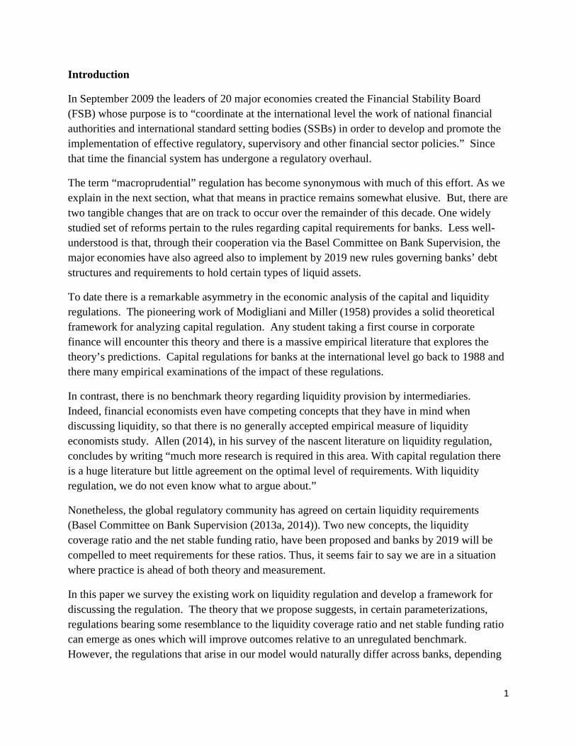
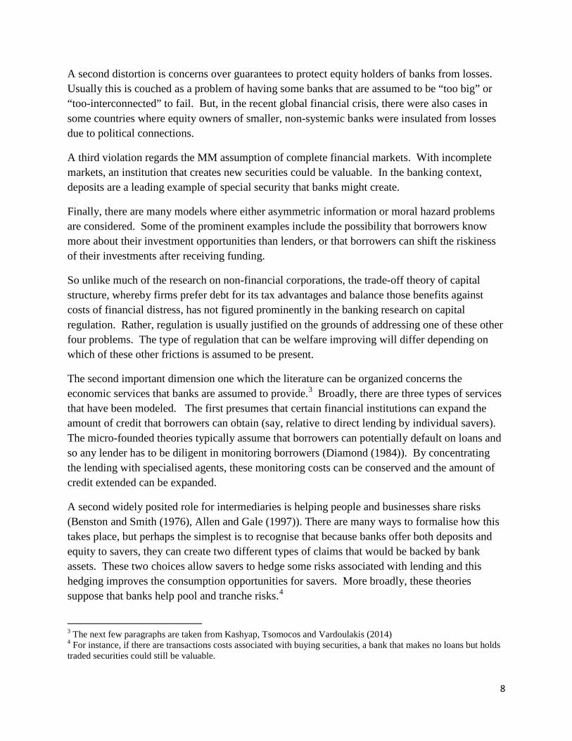
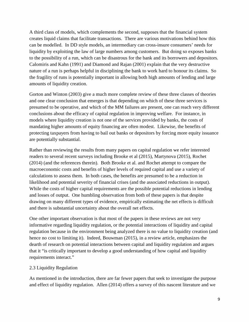
It is worth noting that will most of the literature on liquidity and liquidity regulation label the institutions that that undertake this activity as “banks”. However, as became evident in the global financial crisis this activity is hardly limited to banks. Figure 1, reproduced from Bao, David and Hong (2015) shows the total amount of runnable funding inside the U.S. financial system over the past 30 years.

We draw three conclusions from their estimates that are worth bearing in mind throughout the rest of the discussion. First, there has been a sizable increase in the amount maturity transformation over the last 20 years. From 1995 until 2015, the scale of such activity rose by 50% as measured relative to Gross Domestic Product. Second, as far back as 1985 as much of this activity has occurred outside the banking system as inside it. Third, the decline immediately after the GFC was sizable. The drop in repurchase agreements and money market funds were especially pronounced, but even as a percent of GDP, the level in 2015 is very similar to the level in 2005 (just before the frenzied period ahead of the GFC). Hence, maturity transformation is still happening on a substantial scale even after the GFC and all of the various regulatory reforms that have been introduced.

Given this evidence, we focus only on papers where one of the services of the financial system is to provide liquidity. Among these it is helpful to separate them into papers that model liquidity provision in the same way or similarly to DD, and those that introduce other mechanisms.

11

Figure 1: Bao, David and Han (2015) Estimates of Runnable Funding in the U.S.

Among the DD style models, we focus on three that are closely related to our analysis. Ennis and Keister (2006) have a DD style model (related to Cooper and Ross [1998]) which determines how much liquidity banks need to hold to deter runs. They compute the amount of excess liquidity the bank must hold to buffer it against a run by all depositors, and also determine the optimal amounts to promise depositors. In their model with full information, when depositors desire safe banks, there will be private incentives to hold enough excess liquidity to deter a sunspot-based run. They do not study regulation because there is no need for any under their assumptions, but we will see that some of the same forces that are present in their model arise in ours.

Vives (2014) analyzes a question similar to that in Ennis and Keister (2006): what are the efficient combinations of equity capital and liquidity holdings to make a bank safe when it subject to runs based on private information about its solvency? He studies a global game where a bank can be insolvent or illiquid. The need for regulation is not considered explicitly, but he does examine what capital and liquidity levels would make the bank safer. He finds that capital and liquidity are differentially successful in attending to insolvency and illiquidity. In particular, if depositors are very conservative (and which makes them more inclined to run in the

12

model), increased liquidity holdings which reduce profits by investing more in liquid assets can enhance stability.

Farhi, Golosov, and Tsyvinski (2009) investigate a DD model where consumers need banks to invest and where the consumers can trade bank deposits. Absent a minimum liquidity regulation, it is profitable to free ride on the liquidity held by other banks, because banks offer rates which subsidize those who need to withdraw their deposit early (which is the spirit of Jacklin(1987)). A floor on liquidity holdings removes the incentive for this free riding.

Among the non-DD models, one that is related is Calomiris, Heider, and Hoerova (2014). They have a six period model where banks can potentially engage in risk-shifting so that when banks suffer loan losses they may not be able to honor their deposit contracts. Cash is observable and mandating that banks must have minimum levels of cash reserves can limit the risk-shifting.

Santos and Suraez (2015) examine another role for liquidity when runs occur slowly: it allows time to decide if the bank’s assets are sufficient to imply solvency absent a run. This channel is foreclosed in our set-up with assets which are free of risk.

More generally, our approach is closely related to the mechanism design approach to regulation of monopolists in Baron and Myerson (1982). They also were interested in investigating how regulation could be structured to induce the party being regulated to efficiently use information that is private.

3. Baseline Model

We begin by describing a baseline set up in which the timing and preferences are as in DD. We then modify certain informational assumptions to bound the possible outcomes. Throughout we maintain that there are three dates, T= 0, 1, and 2. The interest rates that bank must offer are taken as given, motivated by a monopoly bank which must meet the outside option of depositors to attract deposits. Equivalently, the single bank can be thought of as representing the overall banking system.

For a unit investment at date 0, the bank offers a demand deposit which pays either r1 at date 1 or r2 at date 2. This effectively offers a gross rate of return r2/r1 between dates 1 and 2 which is equal to the exogenous outside option (such as government bonds) for depositors between these dates. Essentially, the bank offers one period deposits which equal the interest rate on the outside option. We will assume that depositors are sufficiently risk averse that they would like the banking system to supply one period deposits that are riskless. Hence, when we consider interventions they will be designed to deliver as this as the only possible equilibrium.

13

The residual claim after deposits are paid is limited liability equity retained by the banker. All equity payments are made at date 2.5

The bank can invest in two assets with constant returns to scale. One is a liquid asset (which we will interchangeably refer to as the safe asset) that returns R1>0 per unit invested in the previous period. The other is an illiquid asset for which a unit investment at date 0 returns at date 2 an amount that exceeds the return from rolling over liquid assets (R2> R1* R1). The illiquid asset (which we will interchangeably refer to a loan) can be liquidated for θR2 date 1, where θR2< R1 and θ≥0. These restrictions imply that when the bank knows it must make a payment at date 1, it is always more efficient to do that by investing in the safe asset rather than planning to liquidate the loan.

We also assume that banking is profitable even if the bank invests exclusively in the liquid asset, so that 1 1r R≤ and 2

2 1r R≤ . This is a sufficient condition to guarantee that requiring excess liquidity will not make the bank insolvent (though it still will reduce the efficiency of investment). In addition, we assume that bank profits from investing in illiquid assets when depositors hold their deposits for two periods (borrowing short-term repeatedly to fund long-term illiquid investment) is greater than from investing in liquid assets when depositors hold their

deposits for only one period (or 2 1

2 1

r r<R R

). This implies that a bank is most profitable when in

can finance loans returning R2 with deposits for two periods at cost r2 (as compared with financing liquid assets for one period). This second assumption is used only to obtain some results on optimal liquidity holdings.

There are many possible reasons to presume that the illiquid asset can be liquidated for only θR2. For instance, in DD liquidation can be thought of as a non-tradable production technology. Alternatively it could reflect the bank’s lending skills, implying that it would be worth less to a buyer than to the bank because (compared to the bank) the buyer would be able to collect less from a borrower, as in Diamond-Rajan (2001). Nothing in our analysis hinges on why this discount exists, though we do insist that it is operative for everyone in the economy including a potential lender of last resort. Also, our assumption that θ is a constant implies that we are not modeling a situation where the sale price depends only on the amount of remaining liquidity held by potential buyers (as in Bhattacharya-Gale (1987), Allen-Gale (1997) and Diamond (1997)).

For fundamental reasons, a fraction ts of depositors want to withdraw at date 1 and 1-ts want to withdraw at date 2 in state s. The realizations of ts are bounded below by t 0≥ and above byt 1≤ The banker will know the realization of ts when the asset composition choice is made.

This assumption is meant to capture the fact that banks have superior information about their 5 We could introduce another incentive problem for the banker to motive a minimum value of equity at all dates and states, but for now the bank will operate efficiently as long as equity remains positive in equilibrium.

14

customers. Indeed, some early theories of banking supposed that the advantage of tying lending and deposit making was that by watching a customer’s checking account activities a bank could gauge that customer’s creditworthiness (Black(1975)).

Mester, Nakamura and Renault (2007) provide direct evidence supporting the assumption that banks can learn about customer credit needs by monitoring transactions accounts. Drawing on a unique data set from a Canadian bank, they demonstrate the bank is able to infer changes in the value of borrowers’ collateral that is posted against commercial loans by tracking flows into and out of the borrowers’ transaction accounts. At this bank they document that the number of prior borrowings in excess of collateral is an important predictor of credit downgrades and loan write-downs. Most importantly, the bank uses this information in making credit decisions. Loan reviews become longer and more frequent for borrowers with deteriorating collateral.6 In what follows, we make the simplifying assumption ts is always known exactly by the bank, but the analysis also goes through so long as the bank is simply better informed than the depositors and the regulator.

To understand agents’ incentives, note that if the ex-post state is s and there is not a run, a fraction f1=ts will withdraw r1 each, requiring r1ts in date 1 resources, and this will leave a fraction 1-ts depositors at date 2 who are collectively owed r2(1-ts) (in date 2 resources). If we let αs be the fraction of the bank’s portfolio that is invested in the liquid asset and (1-αs) be the portion invested in the illiquid one, then the bank’s profits, and hence its value of equity in general will be

2 1 1 1 1 1 2 1 1 1

1 1 12 1 2 1

2

(1-α )R + (α R f r )R (1 f )r if f r α RValue of equity = (1) (f r -α R ) Max{0, (1-α - )R - (1-f )r } if f r α R

θR

s s s

ss s

- - - ≤ >

Because we are assuming that the bank knows ts, its own self-interest will lead it to make sure to always have enough invested in the liquid asset to cover these withdrawals. So absent a run, the profits are very intuitive and easy to understand. The first term in (1) when 1 1 1f r α Rs≤ represents the returns from the illiquid investment, the second reflects the spread on the safe asset relative to deposits (recognizing that any leftover funds are rolled over), and the third term reflects the funding costs of the remaining two period deposits. When 1 1 1f r α Rs> , the bank needs to pay out more than its liquid assets are worth at date 1. To honor its promises the bank must liquidate illiquid assets worth 2θR each, implying that each unit of withdrawn in excess of 1s Rα removes

2

1θR

loans from the bank’s balance sheet. These loans would each be worth R2 at date 2. For a

6 Norden and Weber (2010) also find that credit line usage, credit limit violations and cash inflows into checking accounts are unusual in the periods preceding defaults by small businesses and individuals in Germany.

15

bank in this situation that can honor all early and late withdrawals the residual profits go to the banker (otherwise the bank is insolvent). Given our assumptions about interest rates and liquidation discounts, if actual withdraws, f1, were known, the bank would choose to hold enough liquid assets to avoid needing to liquidate any loans. We know that at all times, even absent a run in state s, 1 s 1f t r≥ . As a result, the bank will always have an incentive to choose

AIC1s

1

t r αRs

sα ≥ ≡ As a result we refer to AICsα as the automatically incentive compatible liquidity

holding of the bank.

It is interesting to consider what happens when a run is possible. We suppose that a fixed number Δ of the patient depositors are highly likely to see a sunspot. All depositors (and the bank) know Δ and upon seeing the sunspot they must decide whether they believe that the others who see it will decide withdraw their funds early. As mentioned earlier, the sunspot is intended to stand in for general fears about the solvency of the bank, so the inference problem relates to their conjecture about whether others investors might panic. In that case, they have to decide whether to join the run.7 So in general f1> ts is possible.

If the bank will be insolvent with a fraction of withdrawals of any amount less than st +Δ , then

we assume each depositor who sees then sunspot will withdraw and 1 sf =t +Δ . This will give zero to all who do not withdraw, and the goal of bank or its regulator is to prevent this outcome from ever being a Nash equilibrium. We will refer to a bank as unstable if its asset holdings admit the possibility of a run. Alternatively, we refer to a bank as stable if its asset holding eliminate the possibility of a run.

In addition, we will assume that if the bank is exactly solvent at 1 sf =t +Δ , no depositor who does not need to withdraw (and only sees the sunspot) will withdraw. This condition establishes exactly how much liquidity is needed to deter a run (as opposed to providing a floor which must be exceeded). We define the minimum stable amount of liquidity holdings, Stable

sα as the minimum fraction of liquid assets in state s which eliminate the possibility of a run. This implies that a bank with Stable

s sα α≥ will be run-free.

3.1 Complete information.

We presume that depositors desire run-free bank deposits. As a first benchmark, suppose that depositors know all of the choices and information which banks know, and thus observe αs, Δ and ts. In this case, the need to attract deposits will force the bank to make itself run-free. If,

7 Uhlig (2010) shows that partial bank runs in a DD style model can arise if there other types of dispersion in agents’ beliefs. For instance, if depositors are highly uncertainty averse and differ in their estimates of θ that heterogeneity can lead to a partial bank run in his setup.

16

given depositor knowledge of αs, Δ and ts, the bank would remain solvent in a run, then it never is individually rational to react to the sunspot and there will be no runs. Proposition 1 shows that it is possible that the bank will not need to distort its holding of liquidity to implement run-free banking.

( ) ( )

s 1s 1 2 2

1 1 1

1 2

AIC 1s

2 1 1 ss

1 s

1

2

t rt r + (1- )θR - r θR Δr R (equivalently θ ),

r - r θ R R -r t - r R 1-t

t rProposition 1

-Δ

investo

: If the ban

rs will n

k chooses α = , and if

ot run and the bank is stable with

R

t +

α

s

s∆ < ≥

AIC 1s

1

t r= .R

s

AIC

1 1 11

AIC s

12

1

2

1

1 2 So, when

t rthe automatically ince

(f r -α R )Proof: If f r , the bank's equity is positive w

ntive compatible level of initial liquid

hen (1-α -

ity α is chosen (

)R - (1-f )r

α = )

0.θR

R

,

ss

s

Rα> ≥

1

1

s 1 s 11 2 2

1 11

1 2*

s

*

the

t r t rR + (1- )θR - r θR Rvalue of equity is decreasing in f and equal zero when f . Therefore,

r - r θif t +Δ is less than f , then the depositors always know the bank will be solv

=

ent and there is no

Nash equlibrium with a run.QED

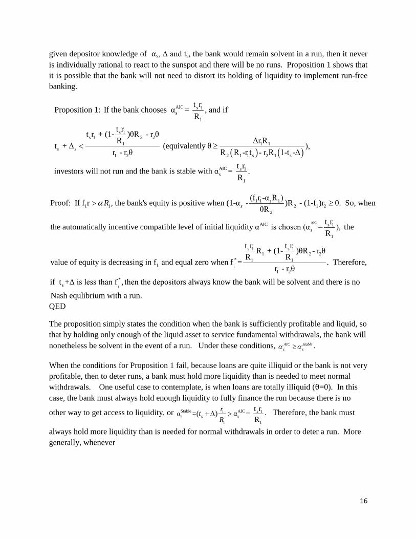
The proposition simply states the condition when the bank is sufficiently profitable and liquid, so that by holding only enough of the liquid asset to service fundamental withdrawals, the bank will nonetheless be solvent in the event of a run. Under these conditions, AIC Stable

s sα α≥ .

When the conditions for Proposition 1 fail, because loans are quite illiquid or the bank is not very profitable, then to deter runs, a bank must hold more liquidity than is needed to meet normal withdrawals. One useful case to contemplate, is when loans are totally illiquid (θ=0). In this case, the bank must always hold enough liquidity to fully finance the run because there is no

other way to get access to liquidity, or 1

1

Stable AIC 1s s

1

=α ( ) t rα = Rs

s Rrt + ∆ > . Therefore, the bank must

always hold more liquidity than is needed for normal withdrawals in order to deter a run. More generally, whenever

17

( ) ( )stable stab

stable

stable

s 1s 1 2 2

1s

1 2

s1ss

1 1s

2 1 1 s 2 1

s

ss

t rt r + (1- )θR - r θ

R or then the bank must increase + to α to

α αdefinitely deter the run, where α is such that

α r - r θ

R + (1t

-+

Δr Rθ<R R -r t - r R 1-t -Δ

t ∆ >

∆ =le

stable

2 2

1 2

1 2 2

1 2s

θR - r θ. This yields

r - r θ

( ) ((1

)

)α

).s st r t r R

RRθ

θ+ ∆ -- - ∆

-

+=

So when it is sufficiently illiquid, merely preparing to service fundamental withdrawals will not

always be enough to deter a run.

This threshold tells us how much liquidity is needed when there is full information such that all variables including ts are known and all parties understand the bank’s incentives. Under the

conditions or Proposition 1, the bank will choose s 1s

1

t rα =R

and no unused liquidity is held from

dates 1 to 2. Because depositors might choose to run and the incentive for this must be removed, this will not be enough liquidity when the conditions for Proposition 1 do not hold. To always deter a possible run, the bank will have to hold Stable

s sαα = .AICsα> This will require that some

unused liquidity, Stable

s 1(α α ) R ( ) 0AICs sU t- ≡ > , to be held from date 1 to 2, after the normal

withdraws are met at date 1. If the bank is free to use all of this unused liquidity if a run should occur, then depositors can see that the liquidity is present and will never choose to run. Once the run is deterred, the liquidity will be in excess of what is needed. This is the simplest example of the benefits of holding unused liquidity or leaving extra taxicabs at the train station.

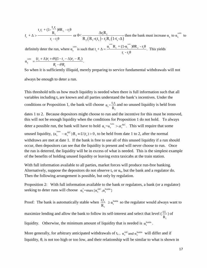
With full information available to all parties, market forces will produce run-free banking. Alternatively, suppose the depositors do not observe ts or αs, but the bank and a regulator do. Then the following arrangement is possible, but only by regulation.

Proposition 2: With full information available to the bank or regulators, a bank (or a regulator) seeking to deter runs will choose * AIC Stable

s s sα =max{α ,α }

Proof: The bank is automatically stable when Stable1 ss

1

r t αR

≥ so the regulator would always want to

maximize lending and allow the bank to follow its self-interest and select that level ( 1 s

1

r tR

) of

liquidity. Otherwise, the minimum amount of liquidity that is needed is Stablesα .

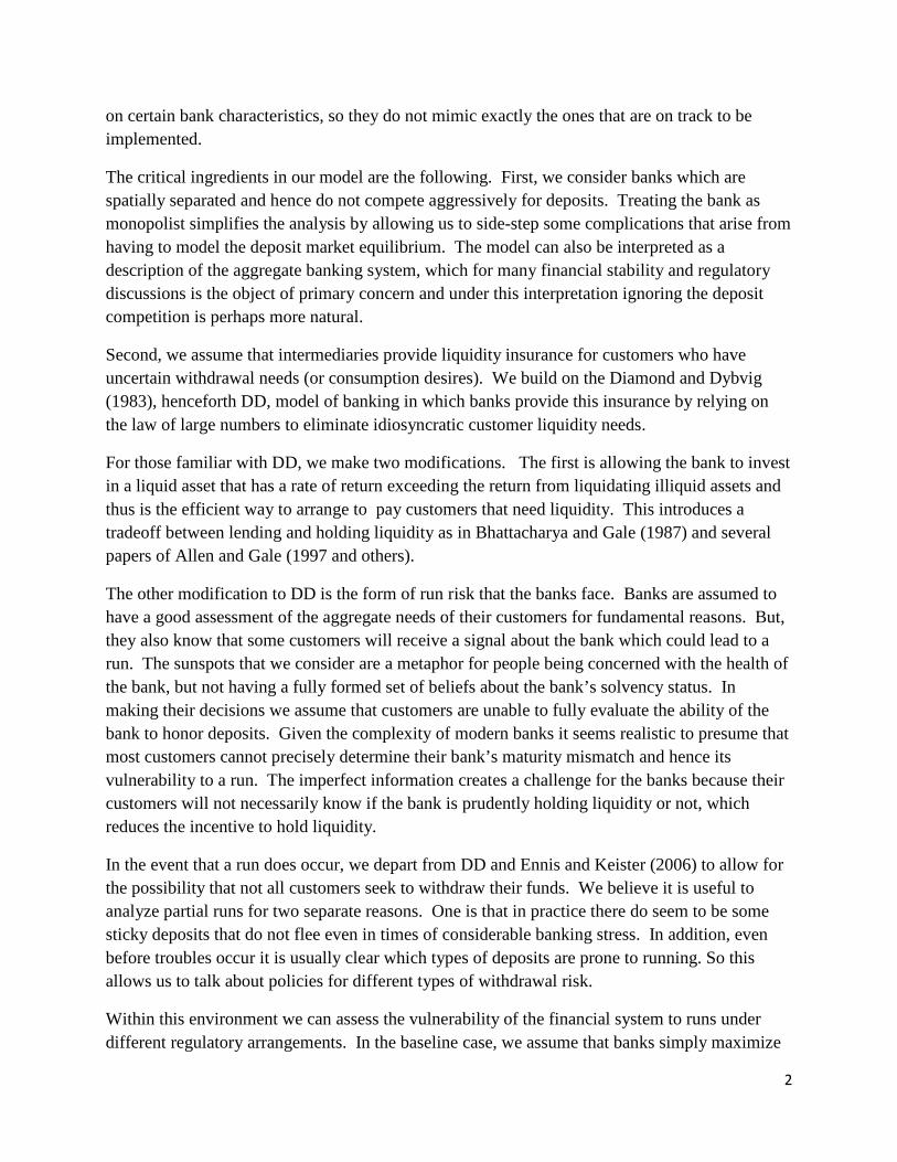
More generally, for arbitrary anticipated withdrawals of ts , StableAICs s αα and will differ and if

liquidity, θ, is not too high or too low, and their relationship will be similar to what is shown in

18

α= fraction

in liquid asset

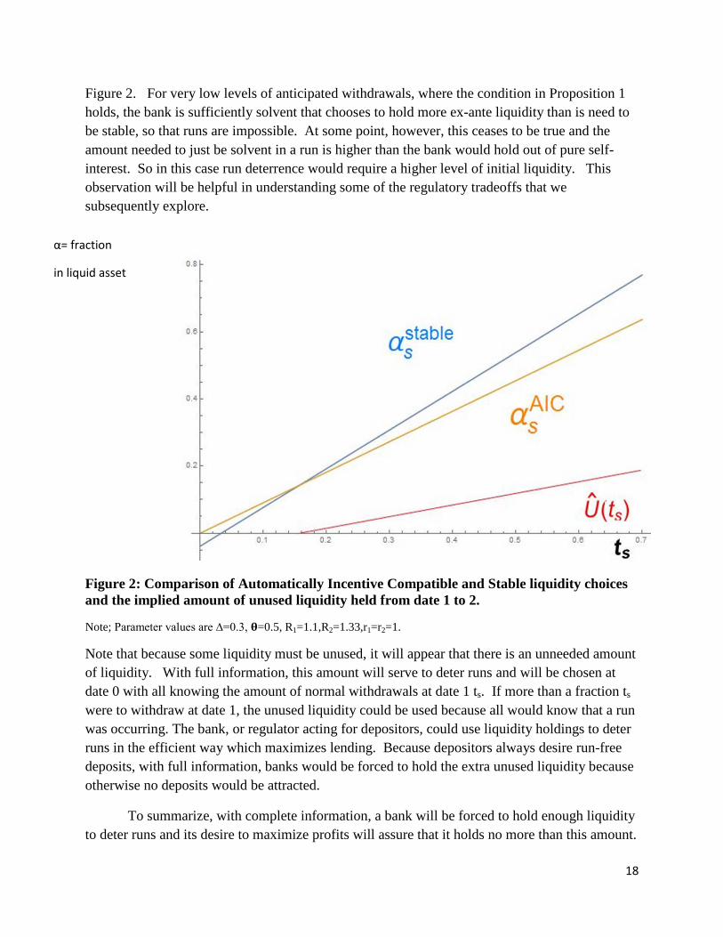
Figure 2. For very low levels of anticipated withdrawals, where the condition in Proposition 1 holds, the bank is sufficiently solvent that chooses to hold more ex-ante liquidity than is need to be stable, so that runs are impossible. At some point, however, this ceases to be true and the amount needed to just be solvent in a run is higher than the bank would hold out of pure self-interest. So in this case run deterrence would require a higher level of initial liquidity. This observation will be helpful in understanding some of the regulatory tradeoffs that we subsequently explore.

Figure 2: Comparison of Automatically Incentive Compatible and Stable liquidity choices and the implied amount of unused liquidity held from date 1 to 2.

Note; Parameter values are ∆=0.3, 𝛉𝛉=0.5, R1=1.1,R2=1.33,r1=r2=1.

Note that because some liquidity must be unused, it will appear that there is an unneeded amount of liquidity. With full information, this amount will serve to deter runs and will be chosen at date 0 with all knowing the amount of normal withdrawals at date 1 ts. If more than a fraction ts

were to withdraw at date 1, the unused liquidity could be used because all would know that a run was occurring. The bank, or regulator acting for depositors, could use liquidity holdings to deter runs in the efficient way which maximizes lending. Because depositors always desire run-free deposits, with full information, banks would be forced to hold the extra unused liquidity because otherwise no deposits would be attracted.

To summarize, with complete information, a bank will be forced to hold enough liquidity to deter runs and its desire to maximize profits will assure that it holds no more than this amount.

19

The next section explains why the complete information benchmark may not be very informative. Once the possibility of incomplete information is considered we can see that arriving at run-free banking can be challenging.

3.2 Incomplete Information: Is it a Problem?

While the full information benchmark is helpful, we think it is too extreme to be realistic. Banks disclosures may be very difficult to interpret. We describe a few compelling reasons to doubt that simply disclosing some information about liquidity holdings will make depositors (or regulators) well-informed about all of these quantities. This suggests that disclosure of such information may not, by itself, force a bank to make the decisions which they would make under complete information.

There is one important situation where incomplete information is not necessarily a problem. Even if there is no disclosure of asset holdings, depositors who know Δ and observe a such ts the conditions of Proposition 1 are satisfied, will know that the bank’s choice will eliminate run-risk

in state s, because AIC Stable1s s

1

t rα = αRs ≥ (the bank is automatically stable in this case). If this was

satisfied for all states, s, a bank would always choose a level of liquid asset holdings which always result in stability even if no one could verify those holdings and if no depositor knew the state s. Whenever this condition is not universally satisfied, the bank’s incentives to hold liquidity will depend on the information available to depositors (or regulators) and on the incentives provided to the bank.

We believe that in most cases a bank’s liquidity choice is not always automatically stable. This suggests that some forms of disclosure or regulation will influence its choice of liquidity. We describe two types of reasons that simple disclosure of liquidity is difficult to interpret. First, if disclosure (or a regulatory requirement) regarding liquidity only applies on some dates (such as the end of an accounting period), the bank can distort the disclosure. Second, even if a liquidity disclosure (or requirement) is on all dates, it is plausible that the bank knows much more about its customers liquidity needs than anyone else, which makes it very difficult to determine if a given level of liquidity is sufficient to make the bank stable and run-free.

3.2.1 Problems with the Periodic Disclosure of Liquidity

One important problem facing depositors is the difficulty in interpreting the kind of accounting data that must be parsed in order to decide whether to join a run. Disclosures that are made on liquidity positions typically occur with a delay and are periodic (such as at the end of a quarter or a fiscal year). The inference problem for depositors can be compounded by the temptation for banks to engage in window dressing of their accounting information.

One eye-opening example of the problem, analyzed in Munyan (2015), is the tendency of (mostly) European banks to disguise borrowing around quarter-end dates. As Munyan (2105)

20

explains, many non-U.S. banks are required to report their accounting information that forms the basis various regulatory ratios only on the last day of the quarter. In the U.S. banks also have to show average daily ratios for critical balance sheet variables which caps the gains from manipulating end-of-quarter data. The non-U.S. banks apparently sell some safe assets just before the end of the quarter and then buy them back shortly afterwards. This transaction allows them to report lower leverage across the quarter-end date.

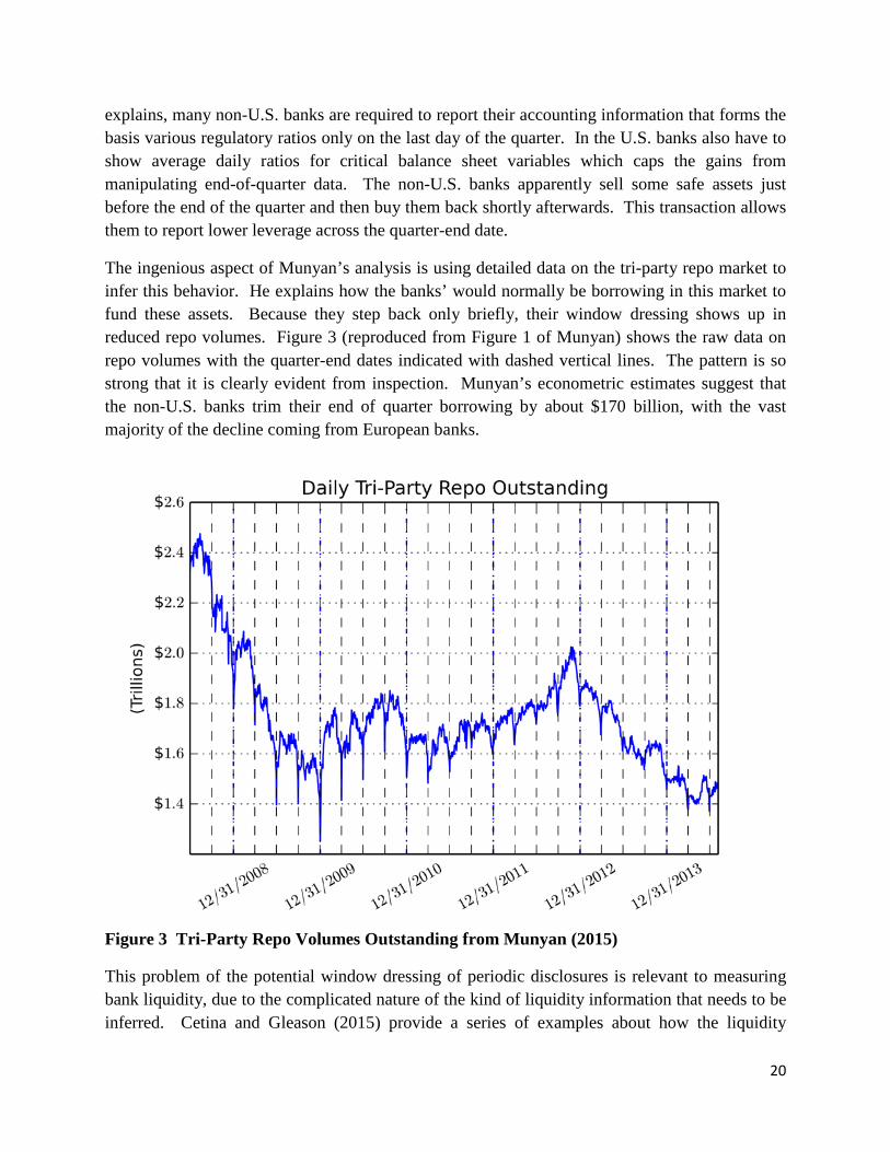
The ingenious aspect of Munyan’s analysis is using detailed data on the tri-party repo market to infer this behavior. He explains how the banks’ would normally be borrowing in this market to fund these assets. Because they step back only briefly, their window dressing shows up in reduced repo volumes. Figure 3 (reproduced from Figure 1 of Munyan) shows the raw data on repo volumes with the quarter-end dates indicated with dashed vertical lines. The pattern is so strong that it is clearly evident from inspection. Munyan’s econometric estimates suggest that the non-U.S. banks trim their end of quarter borrowing by about $170 billion, with the vast majority of the decline coming from European banks.

Figure 3 Tri-Party Repo Volumes Outstanding from Munyan (2015)

This problem of the potential window dressing of periodic disclosures is relevant to measuring bank liquidity, due to the complicated nature of the kind of liquidity information that needs to be inferred. Cetina and Gleason (2015) provide a series of examples about how the liquidity

21

coverage ratio is vulnerable to this type of manipulation. Some of the problems come because of the ability to use repurchase agreements (and reverse repurchase agreements) to move the timing of cash flows. But the rules also distinguish between the assumed levels of liquidity of different asset class and some types of transactions can alter both the numerator and denominator of a ratio in different ways. Moreover, the computations in different jurisdictions vary which further complicates comparisons.

In summary, this possibility for window dressing implies that liquidity disclosures and regulations should hold on all dates rather than being applied periodically. In our model, this will mean that it may be difficult to credibly disclose sα , the initial holding of liquidity, because this could be invested in illiquid loans after the disclosure. Requiring liquidity to be held on all dates (after date 1 in our model) will of course limit its use to meet withdraws of deposits. This again brings back the problem of not allowing the last taxicab to leave the station. In addition, disclosure or regulation of complicated liquidity holdings may require careful auditing (for disclosure) or supervision (for regulation).

3.2.2 Liquidity Disclosures are Difficult to Interpret.

A second challenge facing depositors and regulators in interpreting disclosed information is placing it in appropriate context. Suppose all parties are truthfully told the level of liquid asset holdings in the banking system at a given date (or even on every date). Judging whether these are adequate to service impending withdrawals requires knowledge of how far along a potential run might be on that date and how many normal withdrawals are anticipated. If a bank has a small amount of liquidity after its normal withdraws (of 1t sr in state s), this is very different than if normal withdrawals have not yet occurred. It is possible that very little additional liquidity would be needed if most potential withdrawals have already occurred. How could banks credibly communicate such information? The next section provides a model of this, based on the bank’s private information about the normal level of withdrawals, ts.

3.2.3 A Bank has Private Information about needed Liquidity

Before turning to the details of the model, it is helpful to provide some intuition about how private information possessed by the bank interacts with the incentives of depositors to run. Similar problems arise at both date 0 and date 1 in the model, but we will describe them in turn. One reason for separating out the discussion is because in our framework the most natural analogues to the Basel style regulation can be thought of in terms what they imply as of different dates.

If there is no way to communicate what the bank knows, and it is not automatically stable, then disclosing a level of liquidity at date 0, sα , which would make the bank stable only in some states of nature, ts, will not be adequate completely eliminate runs. In these cases, depositors will have two reasons to be worried. First, in the states of nature where it would not be stable, a run

22

would cause the bank to fail and thus would be self-fulfilling, leading to losses by depositors who did not run.

Second, because depositors do not know ts, a depositor (whom we assume to be very risk averse) who sees a sunspot and worries about a run will always withdraw rather than face losses if the unknown state turns out to be one that makes the bank fail. As a result, a level of liquidity disclosure which is not sufficient to makes a bank run-free for all levels of ts, will lead to runs whenever they are feared, even for the levels of ts where this does not cause bank failure. In the next section, we will explain why a Net Stable Funding Ratio approach to liquidity regulation (which can be mapped into restrictions on date 0 liquidity choices) can be susceptible to such concerns.

Suppose that a positive level of liquidity held at date 1, after withdrawals from a fraction f1 of deposits, is regulated and required. It can also be very difficult to interpret this level when the normal level of withdrawals, ts, is unknown. Any liquidity which must be held from date 1 to date 2 is not available to service withdrawals at date 1. From Proposition 2, we would like to require a level of unused liquidity U(ts) that coincides with the amount specified under full information. This amount would deter runs in state s by being available to be completely used to meet the withdrawals in a run from a fraction ts+∆ of depositors.

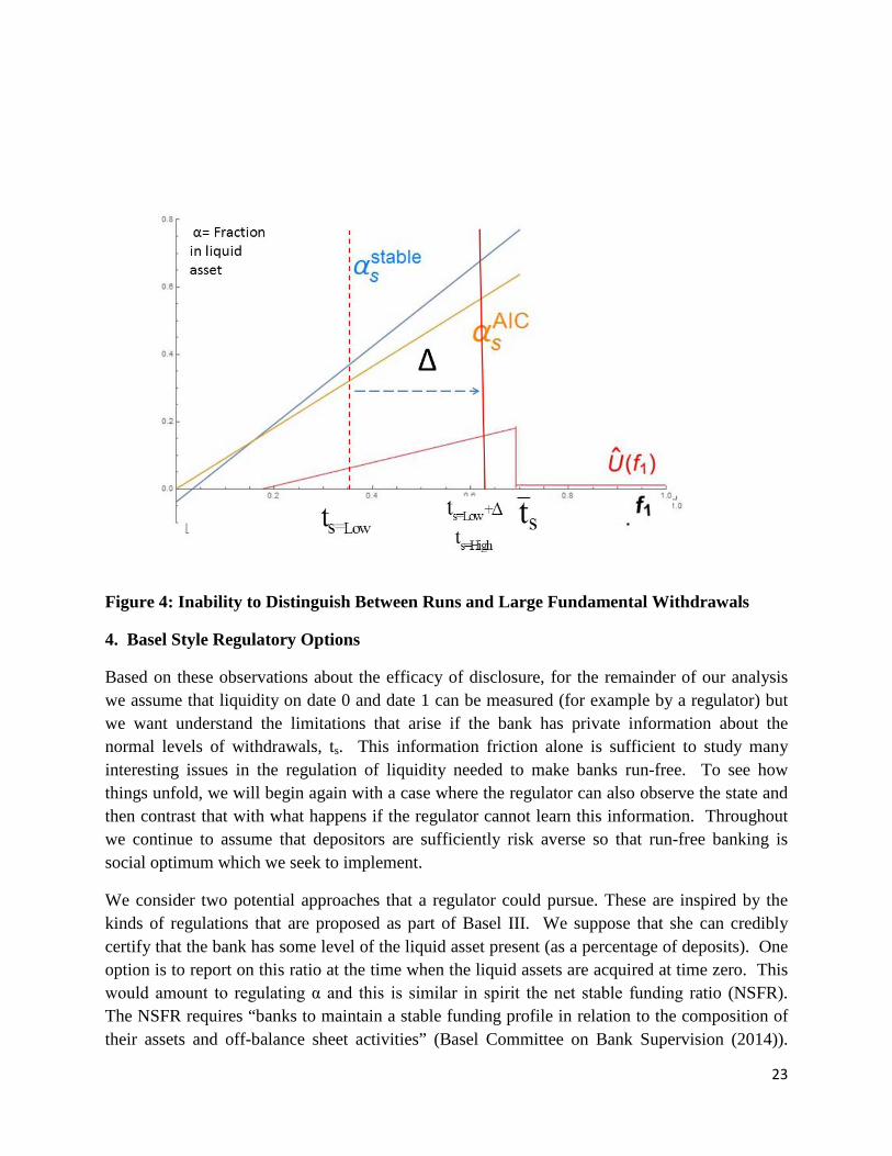
When depositors must guess about the level of normal withdrawals, merely observing the actual outflows in period 1 is not necessarily enough to assure them about the safety of their deposits. To see the problem consider two levels of normal withdrawals, High and Low such that

s=High s=Lowt =t +Δ . A positive level of liquidity which must be held if 1 s=highf =t cannot be released

to meet with the same number of withdrawals during a run with 1 s=lowf =t + ∆ . This is shown in Figure 4. Therefore, the full information level of liquidity required at date 1 cannot be implemented without a way to learn the bank’s information about the normal level of withdrawals, ts. We will show how this is related to the implementation of the Liquidity Coverage Ratio approach to regulating liquidity in the next section.

For the balance of this paper, we assume that liquidity on date 0 and date 1 can be measured (for example by a regulator) but that the bank has private information about the normal levels of withdrawals, ts. This information friction alone is sufficient to study many interesting issues in the regulation of liquidity needed to make banks run-free. If the regulator cannot learn this information, it will constrain the efficiency of regulation.

23

Figure 4: Inability to Distinguish Between Runs and Large Fundamental Withdrawals

4. Basel Style Regulatory Options

Based on these observations about the efficacy of disclosure, for the remainder of our analysis we assume that liquidity on date 0 and date 1 can be measured (for example by a regulator) but we want understand the limitations that arise if the bank has private information about the normal levels of withdrawals, ts. This information friction alone is sufficient to study many interesting issues in the regulation of liquidity needed to make banks run-free. To see how things unfold, we will begin again with a case where the regulator can also observe the state and then contrast that with what happens if the regulator cannot learn this information. Throughout we continue to assume that depositors are sufficiently risk averse so that run-free banking is social optimum which we seek to implement.

We consider two potential approaches that a regulator could pursue. These are inspired by the kinds of regulations that are proposed as part of Basel III. We suppose that she can credibly certify that the bank has some level of the liquid asset present (as a percentage of deposits). One option is to report on this ratio at the time when the liquid assets are acquired at time zero. This would amount to regulating α and this is similar in spirit the net stable funding ratio (NSFR). The NSFR requires “banks to maintain a stable funding profile in relation to the composition of their assets and off-balance sheet activities” (Basel Committee on Bank Supervision (2014)).

24

Loosely speaking, the NSFR can be thought of as forcing banks to match long term assets with long term funding. Our interpretation of this requirement is that the bank is free to violate the requirement temporarily in the future, so it is not always a binding restriction. As a result, it is very much like a requirement that the bank chooses a level of liquid holdings at date 0, αs. From Proposition 2 we know that with complete information a regulation that is bank and state specific can be effective in delivering run-free banking, the question we ask now is what happens in other situations.

Alternatively, a regulator could insist that the bank will always have a certain amount of liquid assets relative to deposits at all times, including after any withdrawals. This kind of regulation is more like the liquidity coverage ratio (LCR). The LCR requires “that banks have an adequate stock of unencumbered high-quality liquid assets (HQLA) that can be converted easily and immediately in private markets into cash to meet their liquidity needs for a 30 calendar day liquidity stress scenario (Basel Committee on Bank Supervision (2013a)).

4.1 A Liquidity Coverage Ratio Regulation

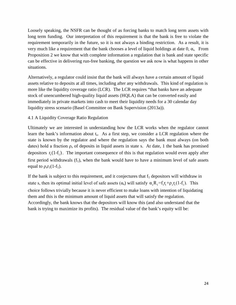
Ultimately we are interested in understanding how the LCR works when the regulator cannot learn the bank’s information about ts. As a first step, we consider a LCR regulation where the state is known by the regulator and where the regulation says the bank must always (on both dates) hold a fraction ρs of deposits in liquid assets in state s. At date, 1 the bank has promised depositors 1 1r (1-f ) . The important consequence of this is that regulation would even apply after first period withdrawals (f1), when the bank would have to have a minimum level of safe assets equal to ρsr1(1-f1).

If the bank is subject to this requirement, and it conjectures that f1 depositors will withdraw in state s, then its optimal initial level of safe assets (αs) will satisfy 1 1 1 1 1α R =f r +ρ r (1-f ).s s This choice follows trivially because it is never efficient to make loans with intention of liquidating them and this is the minimum amount of liquid assets that will satisfy the regulation. Accordingly, the bank knows that the depositors will know this (and also understand that the bank is trying to maximize its profits). The residual value of the bank’s equity will be:

25

1 11 1 1 1

1

1 1 1

1

1 1 12 1

2 1 2

2 1 12 1

2 1

α R -r ρ(α R -f r if f < ,r (1-ρ )

f r -α R +ρ (1-f ) α R -r ρ((1-α )- )R +(ρ R -r )(1-f ) if f and if θR r (1-ρ )

E (f ;.,

)R +(1-α )R -(1-f )r

ρ)=

s ss

s

s s s ss s

s

s

≥

1 2 1 1 21

1 1 1 2

1 2 1 11

α R +(1-α )θR -ρ r (1-θR )-r θ f ,r -ρ r (1-θR )-r θ

α R +(1-α )θR -ρ r (1-θR0 if f >

s s s

s

s s s

≤

2

1 1 1 2

)-r θ . r -ρ r (1-θR )-r θs

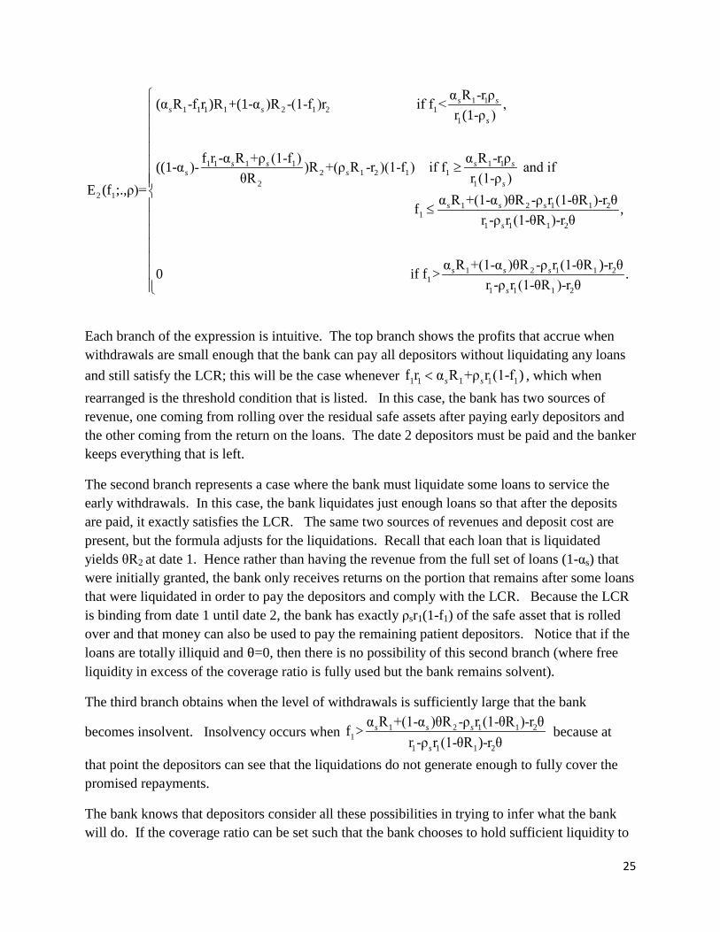
Each branch of the expression is intuitive. The top branch shows the profits that accrue when withdrawals are small enough that the bank can pay all depositors without liquidating any loans and still satisfy the LCR; this will be the case whenever 1 1 11 1f r α R +ρ (1 fr - )s s< , which when rearranged is the threshold condition that is listed. In this case, the bank has two sources of revenue, one coming from rolling over the residual safe assets after paying early depositors and the other coming from the return on the loans. The date 2 depositors must be paid and the banker keeps everything that is left.

The second branch represents a case where the bank must liquidate some loans to service the early withdrawals. In this case, the bank liquidates just enough loans so that after the deposits are paid, it exactly satisfies the LCR. The same two sources of revenues and deposit cost are present, but the formula adjusts for the liquidations. Recall that each loan that is liquidated yields θR2 at date 1. Hence rather than having the revenue from the full set of loans (1-αs) that were initially granted, the bank only receives returns on the portion that remains after some loans that were liquidated in order to pay the depositors and comply with the LCR. Because the LCR is binding from date 1 until date 2, the bank has exactly ρsr1(1-f1) of the safe asset that is rolled over and that money can also be used to pay the remaining patient depositors. Notice that if the loans are totally illiquid and θ=0, then there is no possibility of this second branch (where free liquidity in excess of the coverage ratio is fully used but the bank remains solvent).

The third branch obtains when the level of withdrawals is sufficiently large that the bank

becomes insolvent. Insolvency occurs when 1 2 1 1 21

1 1 1 2

α R +(1-α )θR -ρ r (1-θR )-r θf r -ρ r (1-θR r θ

>)-

s s s

s

because at

that point the depositors can see that the liquidations do not generate enough to fully cover the promised repayments.

The bank knows that depositors consider all these possibilities in trying to infer what the bank will do. If the coverage ratio can be set such that the bank chooses to hold sufficient liquidity to

26

remain solvent during a run, then runs will be deterred. Proposition 3 examines the outcomes if the bank faces a state contingent liquidity coverage ratio in state s, ρ [0,1]s ∈ .

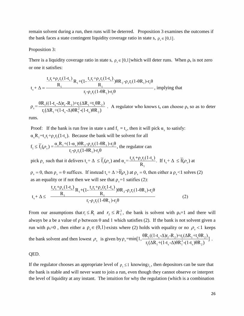
Proposition 3:

There is a liquidity coverage ratio in state s, ρ [0,1]s ∈ which will deter runs. When ρs is not zero or one it satisfies:

s 1 s s 1 s

1 1

1 11 2 1 1 2

s1 1 1 2

r rR +(1- )θR -ρ r (1-θR )t r +ρ (1-t ) t r +ρ ( -r θt + Δ

r -ρ r (1-

1

θR )

t )R R

-r θ

-s

s

ss

= , implying that

1 s 2 2 1 1 s 22

1 1 s 1 s 2

θR ((1-t -Δ)r -R )+r (ΔR +t θR )ρ =r (ΔR +(1-t -Δ)θR (1-t )- θR )s . A regulator who knows ts can choose ρs so as to deter

runs.

1

1 2 1 1 21

1

1 s

1 1 s

1

Proof: If the bank is run free in state s and f = t , then it will pick α to satisfy: α R =t r +ρ r

α R +(1-α )θR -ρ r (1-θR )-r θfr -

(1-t ). Because the bank will be solvent for all

ρ

f ( ) = s

s

s s s

ss s

s

r≤

s 1 s1

1

1 1 2

1s s

s

t r +ρ (1-t )f ( ) and α = .

, the regulator can r (1-θR )-r θ

rpick ρ such that it delivers t + Δ t + Δ

ρ 0, then ρ 0 suffices. If instead t + Δ > ρ 0, then either a ρ <

If f( ) at R

f( ) at

s

s s s s

ss s s

s

r r

r

≤ ≤

= = =

1s 1 s s 11

s

12 1 1 2

s1 2

1

1 1

t r +ρ (

1 solves (2) as an equality or if not then we will see that ρ =1 satifies (2):

rR +(1- )θR -ρ r (1-θR )-r θ t + Δ (2)

r -

1-t ) t r +ρ ( 1-t )R R

ρ r (1-θR )-r θ

s s

s

s

s

≤

From our assumptions that 1 1r R≤ and 22 1r R≤ , the bank is solvent with ρs=1 and there will

always be a be a value of ρ between 0 and 1 which satisfies (2). If the bank is not solvent given a run with ρs=0 , then either a ρ (0,1)s ∈ exists where (2) holds with equality or no 1sr < keeps

the bank solvent and then lowest sr is given by 1 s 2 2 1 1 s 22

1 1 s 1 s 2

θR ((1-t -Δ)r -R )+r (ΔR +t θR )ρ =min[1, ]r (ΔR +(1-t -Δ)θR (1-t )θR- )s .

QED.

If the regulator chooses an appropriate level of ρ 1s ≤ knowing st , then depositors can be sure that the bank is stable and will never want to join a run, even though they cannot observe or interpret the level of liquidity at any instant. The intuition for why the regulation (which is a combination

27

of a rule which can be enforced and credibly auditing) is sufficient to foreclose a run, even when the bank’s liquidity choice is unobservable to depositors, is straightforward. The LCR forces the bank to invest in more liquid assets than it would voluntarily prefer to hold and the depositors know that the regulator is doing this to try to prevent runs. The bank’s own self-interest continues to insure that it plans to always hold enough liquid assets to cover its anticipated fundamental withdrawals and we are assuming that it can do that perfectly. Consequently, knowing that the extra liquidity cannot be avoided removes the incentive to run.

Importantly, once the run has been prevented the liquidity still will have to remain on the bank’s balance sheet. So, under these assumptions it is beneficial to force the last taxi cab to always remain at the train station.

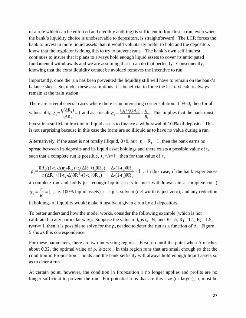
There are several special cases where there is an interesting corner solution. If θ=0, then for all

values of ts, 1 1

1 1

r (ΔR )ρ = 1r ΔRs = and as a result s 1 1 s 1

1 1

t r + (1-t )Rsr r

Rα = = . This implies that the bank must

invest in a sufficient fraction of liquid assets to finance a withdrawal of 100% of deposits. This is not surprising because in this case the loans are so illiquid as to have no value during a run.

Alternatively, if the asset is not totally illiquid, θ>0, but 1 1r R 1= = , then the bank earns no spread between its deposits and its liquid asset holdings and there exists a possible value of ts such that a complete run is possible, st +Δ=1 , then for that value of st

1 s 2 2 1 1 s 2 s 22

1 1 s 1 s 2 s 2

θR ((1-t -Δ)r -R )+r (ΔR +t θR ) Δ-(1-t )θRρ = 1r (ΔR +(1-t -Δ)θR (1-t )θR Δ- (1-t )) - θRs = = . In this case, if the bank experiences

a complete run and holds just enough liquid assets to meet withdrawals in a complete run (1

1

1srR

α = = , i.e. 100% liquid assets), it is just solvent (net worth is just zero), and any reduction

in holdings of liquidity would make it insolvent given a run by all depositors.

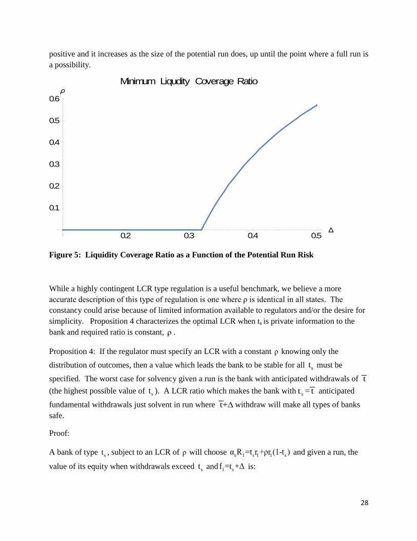
To better understand how the model works, consider the following example (which is not calibrated in any particular way). Suppose the value of ts is ts= ½, and θ= ½, R1= 1.1, R2= 1.5, r1=r2= 1, then it is possible to solve for the ρs needed to deter the run as a function of Δ. Figure 5 shows this correspondence.

For these parameters, there are two interesting regions. First, up until the point when Δ reaches about 0.32, the optimal value of ρs is zero. In this region runs that are small enough so that the condition in Proposition 1 holds and the bank selfishly will always hold enough liquid assets so as to deter a run.

At certain point, however, the condition in Proposition 1 no longer applies and profits are no longer sufficient to prevent the run. For potential runs that are this size (or larger), ρs must be

28

positive and it increases as the size of the potential run does, up until the point where a full run is a possibility.

Figure 5: Liquidity Coverage Ratio as a Function of the Potential Run Risk

While a highly contingent LCR type regulation is a useful benchmark, we believe a more accurate description of this type of regulation is one where ρ is identical in all states. The constancy could arise because of limited information available to regulators and/or the desire for simplicity. Proposition 4 characterizes the optimal LCR when ts is private information to the bank and required ratio is constant, ρ .

Proposition 4: If the regulator must specify an LCR with a constant ρ knowing only the

distribution of outcomes, then a value which leads the bank to be stable for all st must be

specified. The worst case for solvency given a run is the bank with anticipated withdrawals of t (the highest possible value of st ). A LCR ratio which makes the bank with t =ts anticipated

fundamental withdrawals just solvent in run where t+∆withdraw will make all types of banks safe.

Proof:

A bank of type st , subject to an LCR of ρ will choose s 1 s 1 1 sα R =t r +ρr (1-t ) and given a run, the

value of its equity when withdrawals exceed st and 1 sf =t +Δ is:

0.2 0.3 0.4 0.5

0.1

0.2

0.3

0.4

0.5

0.6

Minimum Liqudity Coverage Ratio

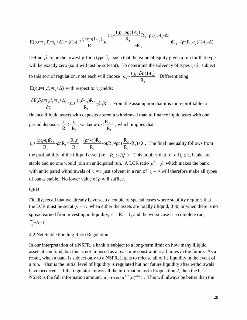
29

s 1 1 ss 1 1 1 s

s 1 1 s 1s 1 s 2 1 1 2 s

1 2

t r +ρr (1-t )t r - R +ρr (1-t -Δ)t r +r ρ(1-t ) RE(ρ,t=t ,f =t +Δ) = ((1-( )- )R +(ρr R -r )(1-t -Δ)

R θR

Define r̂ to be the lowest ρ for a type st̂ , such that the value of equity given a run for that type will be exactly zero (so it will just be solvent). To determine the solvency of types s

ˆt <t s subject

to this sort of regulation, note each will choose s 1 1 ss

1

ˆt r + r (1-t . )α =Rr Differentiating

s 1 sE( ,t=t ,f =t )ˆ +Δr with respect to st yields:

s 1 s 1 22 1

s 11

1E( ,t=t ,f =t +Δ) (r -r )R=r + -ˆ ˆ ˆr R

t Rr r r∂

∂ . From the assumption that it is more profitable to

finance illiquid assets with deposits absent a withdrawal than to finance liquid asset with one

period deposits, 1 2 2 12

1 2 1

r r R r> , we know r <R R R

, which implies that

1 1 2 1 1 2 22 1 1 1 1

1 1 1

2 11 1

1

(ρr -r )R (ρr -r )R Rr + -ρr R r< + =ρr (R -ρr R -RR R R

)<0R

. The final inequality follows from

the profitability of the illiquid asset (i.e., 22 1R R> ). This implies that for all s

ˆt t≤ , banks are

stable and no one would join an anticipated run. A LCR ratio * ˆr r= which makes the bank with anticipated withdrawals of t = ts just solvent in a run of st + ∆will therefore make all types of banks stable. No lower value of ρ will suffice.

QED

Finally, recall that we already have seen a couple of special cases where stability requires that the LCR must be set at 1r = : when either the assets are totally illiquid, θ=0, or when there is no

spread earned from investing in liquidity, 1 1r R 1= = , and the worst case is a complete run,

st +Δ=1 .

4.2 Net Stable Funding Ratio Regulation

In our interpretation of a NSFR, a bank is subject to a long-term limit on how many illiquid assets it can fund, but this is not imposed as a real-time constraint at all times in the future. As a result, when a bank is subject only to a NSFR, it gets to release all of its liquidity in the event of a run. That is the initial level of liquidity is regulated but not future liquidity after withdrawals have occurred. If the regulator knows all the information as in Proposition 2, then the best NSFR is the full information amount, * AIC stable

s sα =max{α ,α } . This will always be better than the

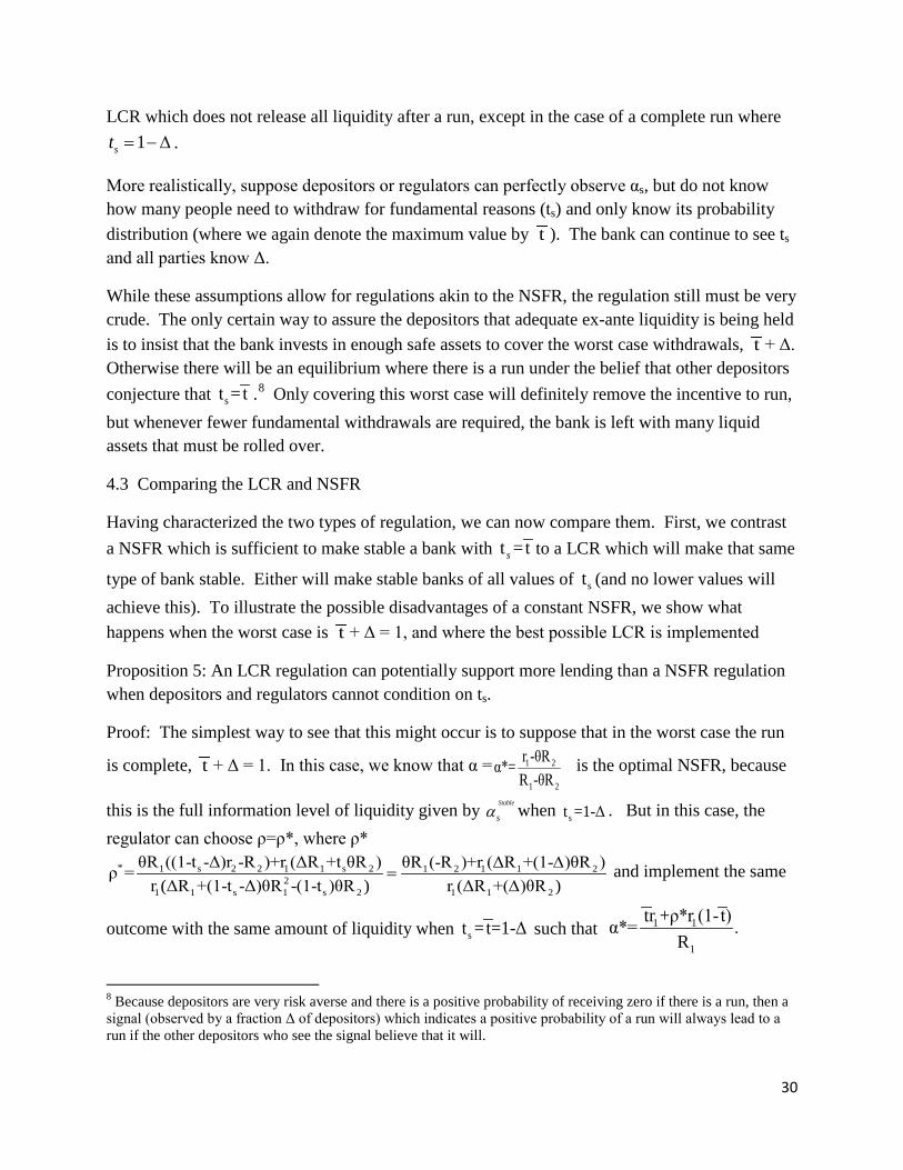
30

LCR which does not release all liquidity after a run, except in the case of a complete run where 1st = -∆ .

More realistically, suppose depositors or regulators can perfectly observe αs, but do not know how many people need to withdraw for fundamental reasons (ts) and only know its probability distribution (where we again denote the maximum value by t ). The bank can continue to see ts and all parties know Δ.

While these assumptions allow for regulations akin to the NSFR, the regulation still must be very crude. The only certain way to assure the depositors that adequate ex-ante liquidity is being held is to insist that the bank invests in enough safe assets to cover the worst case withdrawals, t + Δ. Otherwise there will be an equilibrium where there is a run under the belief that other depositors conjecture that st = t .8 Only covering this worst case will definitely remove the incentive to run, but whenever fewer fundamental withdrawals are required, the bank is left with many liquid assets that must be rolled over.

4.3 Comparing the LCR and NSFR

Having characterized the two types of regulation, we can now compare them. First, we contrast a NSFR which is sufficient to make stable a bank with t = ts to a LCR which will make that same

type of bank stable. Either will make stable banks of all values of st (and no lower values will achieve this). To illustrate the possible disadvantages of a constant NSFR, we show what happens when the worst case is t + Δ = 1, and where the best possible LCR is implemented

Proposition 5: An LCR regulation can potentially support more lending than a NSFR regulation when depositors and regulators cannot condition on ts.

Proof: The simplest way to see that this might occur is to suppose that in the worst case the run

is complete, t + Δ = 1. In this case, we know that α = 1 2

1 2

-α*Rr θR=

-θRis the optimal NSFR, because

this is the full information level of liquidity given by Stable

sα when st =1-Δ . But in this case, the regulator can choose ρ=ρ*, where ρ*

* 1 s 2 2 1 1 s 2 1 2 1 1 22

1 1 s 1 s 2 1 1 2

θR ((1-t -Δ)r -R )+r (ΔR +t θR ) θR (-R )+r (ΔR +(1- )θR )ρ =r (ΔR +(1-t -Δ)θR (1-t )θR r (ΔR +( ) R- ) )θ

∆=

∆ and implement the same

outcome with the same amount of liquidity when st = t=1-Δ such that 1 1

1

tr +ρ*r (1-t)α*= .R

8 Because depositors are very risk averse and there is a positive probability of receiving zero if there is a run, then a signal (observed by a fraction Δ of depositors) which indicates a positive probability of a run will always lead to a run if the other depositors who see the signal believe that it will.

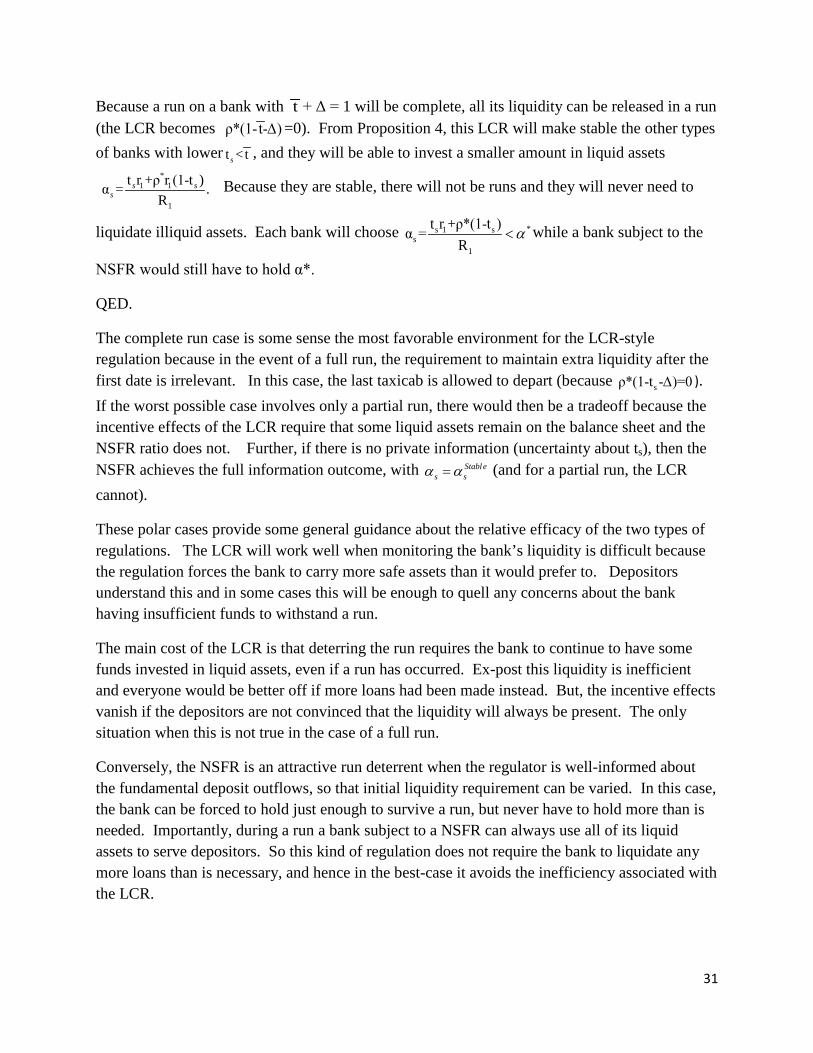
31

Because a run on a bank with t + Δ = 1 will be complete, all its liquidity can be released in a run (the LCR becomes ρ*(1-t- )∆ =0). From Proposition 4, this LCR will make stable the other types of banks with lower t <ts , and they will be able to invest a smaller amount in liquid assets

*1 1

1

t r +ρ r (1-α t )= .R

s ss

Because they are stable, there will not be runs and they will never need to

liquidate illiquid assets. Each bank will choose *s 1 ss

1

t r +ρ*(1-t )α =R

α< while a bank subject to the

NSFR would still have to hold α*.

QED.

The complete run case is some sense the most favorable environment for the LCR-style regulation because in the event of a full run, the requirement to maintain extra liquidity after the first date is irrelevant. In this case, the last taxicab is allowed to depart (because sρ*(1-t - )=0∆ ). If the worst possible case involves only a partial run, there would then be a tradeoff because the incentive effects of the LCR require that some liquid assets remain on the balance sheet and the NSFR ratio does not. Further, if there is no private information (uncertainty about ts), then the NSFR achieves the full information outcome, with Stabl e

s sα α= (and for a partial run, the LCR cannot).

These polar cases provide some general guidance about the relative efficacy of the two types of regulations. The LCR will work well when monitoring the bank’s liquidity is difficult because the regulation forces the bank to carry more safe assets than it would prefer to. Depositors understand this and in some cases this will be enough to quell any concerns about the bank having insufficient funds to withstand a run.

The main cost of the LCR is that deterring the run requires the bank to continue to have some funds invested in liquid assets, even if a run has occurred. Ex-post this liquidity is inefficient and everyone would be better off if more loans had been made instead. But, the incentive effects vanish if the depositors are not convinced that the liquidity will always be present. The only situation when this is not true in the case of a full run.

Conversely, the NSFR is an attractive run deterrent when the regulator is well-informed about the fundamental deposit outflows, so that initial liquidity requirement can be varied. In this case, the bank can be forced to hold just enough to survive a run, but never have to hold more than is needed. Importantly, during a run a bank subject to a NSFR can always use all of its liquid assets to serve depositors. So this kind of regulation does not require the bank to liquidate any more loans than is necessary, and hence in the best-case it avoids the inefficiency associated with the LCR.

32

Once the regulator does not have good knowledge about the fundamental needs of the depositors, using the NSFR becomes less efficient. In this case, depositors cannot generally be confident that the bank will have a portfolio that guarantee solvency in all cases. The best the regulator can, therefore, accomplish is to protect against a worst-case set of withdrawals. This can remove the incentive to run, but doing so will mean that all but the worst case the bank over-invests in safe assets. The LCR potentially is less distorting in this case.

This intuition suggests that the relative advantages of the two approaches to regulation will hinge on two considerations. One is the variability of potential fundamental withdrawal requirements. When ts fluctuates considerably, then regulation that relies on a fixed value of α will only deter runs if the liquidity requirement is set high enough to cover the worst case outcome. When the worst case does not materialize, this will result in the banking holding surplus liquidity. Because the LCR regulation exploits the bank’s knowledge about impending withdrawals and relies on its incentives to plan for these withdrawals, variability of ts is not as severe a problem for this kind of regulation.

The other consideration is the size of the runs that are possible. The Achilles’ heel of the LCR is that is that even after a run has taken place, the bank must continue to hold liquid assets. The NSFR avoids this (ex-post) inefficiency because all the liquid assets that the bank has can be used in the event of a run. So if runs are never complete, the inefficiency associated with the LCR will be at a disadvantage.

It strikes us that the information requirements that would favor the NSFR are relatively onerous. One of the most difficult challenges in a real-time crisis is gauging the extent of a run. In that case, even if it possible to verify and certify that some liquid assets are present at any given point in time, it make be difficult to forecast whether they will be adequate to meet potential subsequent withdrawals. Hence releasing all liquidity on hand can be risky.

One can see a further disadvantage of the NSFR by introducing the possibility that the bank can secretly alter its liquidity holdings after meeting the NSFR, and this can happen at date 0. This is similar to window dressing when liquidity must be reported only at the end of a calendar year. In this case, liquidity must be disclosed at every date and there must be a future commitment to hold liquidity. The LCR is just such a commitment. It does not do as well as the full information commitment, but it does succeed in forcing the bank to remain free of runs (while a NSFR single disclosure will not).

5. Extensions

Having characterized the properties of Basel style regulations in this model, we now discuss the implications of extending the model in two directions. First, there is no reason to restrict regulations to only look like the NSFR and the LCR, so it makes sense to expand the range of regulatory tools considered. Diamond and Kashyap (2016) provide a complete analysis of how

33

to optimally regulate liquidity in this kind of a model and we begin with a review of those results.

Second, we discuss several of the issues that arise if the bank faces capital regulation. Allowing savers to have a choice between investing in deposits and equity greatly complicates the model. Part of the complication comes because our model abstracts from asset risk, and many of the benefits of capital regulation arise from creating a buffer against loan losses so that any discussion of capital without asset risk is necessarily incomplete. Nonetheless, there are a couple of interesting possible comparisons between capital and liquidity regulation that can be made even without developing a full blown model.

5.1 Optimal Regulation of Liquidity

Stepping away from the Basel approach, how should liquidity optimally be regulated in this kind of environment? To find the most efficient set of choices which can be implemented, we describe the results from undertaking a mechanism design analysis.9 This will achieve the best outcome by providing incentives for the bank to reveal to a regulator the information needed to implement run-free banking most efficiently. Proposition 2 already describes the full- information choices and it turns out that these can be implemented with the optimal regulation.

To understand what happens where ts is known only to the bank, we describe a mechanism to which accounts for this information asymmetry and still induces the bank to make efficient choices. The challenge in this situation is that a bank with private information about ts could have an incentive to misreport ts. The condition for efficient investment from the bank’s point of

view without a run remains 1 ss

1

r tα =R

. When the conditions of Proposition 1 regarding the range

of possible withdrawals are satisfied, this level of liquidity automatically leads to a stable, run-free bank. This is what both the bank and its depositors desire and runs will be avoided without any regulation or even any disclosure.

When the bank is not automatically stable, to make it incentive compatible to honestly report st , the bank must be provided an incentive for reporting high levels of anticipated withdrawals that offsets any increased profits that could arise from underreporting. The potential gains from underreporting come from making more loans and hence having less unused liquidity which is held after normal withdrawals occur. Diamond and Kashyap (2016) prove that under our assumptions there is a way to implement the full-information choice of *

sα (from Proposition 2) and which is similar to, but not exactly the same as a liquidity coverage ratio requirement.

9 The analysis here is a special case of the more general treatment in Diamond and Kashyap (2016).

34

This is possible whenever the regulator has sufficient tools to penalize the banker when actual withdrawals deviate from those that the banker reports are anticipated. These tools share the feature that they eliminate the profits that accrue from underreporting. There are various tools that can achieve this outcome. For instance, one approach is to place limits on compensation whenever reports turn out to be inaccurate (to reduce spoils from underreporting). Another strategy is to deploy fines that would be tied to the use of the supposedly required liquidity given the report. If such tools exist then the regulator can require the bank to hold *

sα , can punish any cases where the unused liquidity after the withdrawals departs from what would be needed when the bank is run-free (i.e. when actual withdrawals, f1, deviate from what the bank reports as anticipated withdrawals, ts), but also allow the bank to use the extra liquidity if a run were to occur.

In other words, it is possible to implement the full-information outcomes because if the bank can be induced to be run-free, the actual withdrawals, f1, will be exactly equal to the (state-contingent) fraction of normal withdrawals, ts. In essence, an honestly reported value of ts allows the regulator to determine whether the realized withdrawal f1 is or is not due to a run and release liquidity only in a run. The critical decision by the regulator is to carefully choose how much mandated excess liquidity must be held in all circumstances to create the right incentives for the banker to truthfully report anticipated fundamental withdrawals. Diamond and Kashyap (2016) characterize these choices under various assumptions about the nature of run risk.

The formal mechanism design problem in Diamond and Kashyap (2016) solves for the optimal mechanism by looking for the one where the bank is given incentives to honestly report its private information to the regulator and the regulator uses the honestly reported information to choose a run-free level of liquidity to make the bank stable. Once the bank is run-free, any misreporting of ts by the bank will be measured by a level of withdrawals, f1, which differ from ts. Assessing a sufficiently large penalty (such as driving the banker’s compensation to zero without imposing losses on depositors) for such a misreport will provide incentives for accurate reporting without the need to distort liquidity holding away from the full-information level.

As in the analysis in this paper, the full-information level of liquidity results in excess liquidity held from date 1 to date 2, but with the optimal mechanism all of this liquidity can always be used if a run should occur. While the excess liquidity is available for use, because it deters runs, it is in fact never needed. Returning to our metaphor, the last taxicab is allowed to leave the station, but in equilibrium there are enough cabs such that some always remain at the station.

5.2 Integrating Liquidity Regulation with Lender of Last Resort Policy

If the regulator can also serve as a lender of last resort, then the efficient mechanism, that we just described above, can be implemented by requiring a level of liquidity holdings which depends on the quantity of deposits. This is essentially a generalized LCR. In this case, no actual report of anticipated withdrawals, ts, is required. This is implemented by requiring the amount of unused

35

liquidity at date 1 (to be held until date 2) equal to the full information level from Proposition 2, sStableα , which is given by U(f1=ts)= 1Max[0, ]Rs

Stable AICsα α- , and allowing the bank to use this

liquidity in a run, but with a penalty which drives banker compensation to zero in that case.

The goal from this this policy is to induce the bank to always use its private information to choose to hold just enough liquidity to make sure that after normal withdrawals, ts, it will meet the requirement, U(f1=ts). This is the equal to the investment in liquidity from the full-information level presented in Proposition 2.

To accomplish this outcome, liquidity requirements and lender of last resort policy should be integrated in the following way. Banks are forced to hold the specified amount of liquidity but are allowed to borrow against it for use during a run. If there is a sufficient penalty to the bank for violating its liquidity requirement, the bank will hold the specified amount of liquidity and will never use borrowing to meet normal withdrawals. As a result, the run will be deterred and the extra liquidity need not be borrowed against.

Remarkably, there is historical precedent for this sort of policy: the original United States Federal Reserve Act prohibited dividend payments for banks which were in violation of the reserve (liquidity) requirement. In that period, most banks were closely held, implying that a dividend was a significant part of management compensation. This policy is not necessarily akin to charging a high interest rate for such borrowing, because a penalty rate could be so severe that it might make the bank fail due to a run (making the bank unstable and defeating the purpose of holding extra liquidity).

Note that this type of lender of last resort lends against liquid assets, allowing them to be used during a crisis while providing incentives to get the bank to hold the higher level of liquidity needed to make it stable. This lending does not have moral hazard of inducing the bank to hold excessive amounts of illiquid assets (as described in Bagehot (1873), Goodfriend and King (1988) and Diamond and Rajan (2012)). It may appear pointless to lend against liquid assets, but the ability to penalize the bank for such the borrowing induces the bank to make the proper ex-ante liquidity choice. Once the liquidity is in place, its existence can deter bank runs. Finally, notice that if the lender of last resort acquired (or lent against) illiquid assets and could then only recover their illiquid value, 2θR if the bank were to fail, then lending an amount in excess of this value could distort bank incentives and lead to losses by the lender of last resort. Lending against liquid assets has no such problem.

To summarize, the optimal mechanism induces a bank to hold excess liquidity but allows access to it during a run. The robust conclusion from this analysis is that the optimal regulation requires less unused liquidity than the simple Basel style regulations because the excess liquidity can be released if a run should occur. If there are additional constraints on what the regulator can do, which limit the ability to release this liquidity, then a regulation like the LCR could be nearly

36

optimal. If all liquidity cannot be released in a run, then the best regulations will have the property that as anticipated withdrawals rise, the amount of required surplus liquidity falls.

5.3 Interactions between Capital and Liquidity Regulations

Finally, it is worth noting several observations about interactions between capital and liquidity regulation. In our baseline model, there is no credit risk associated with loans, so the usual arguments for capital requirements do not hold. Generically, however, the incentive to run is still related to depositors’ assessments about the solvency of the bank so the presence of equity could still matter.

The role that capital would play in deterring a run is subtle. On the one hand, if the bank issued capital (non-demandable liabilities) and invested the proceeds in loans, this can leave the bank more solvent when a fixed number of deposits are withdrawn, moving the bank to a situation where it is solvent during a (potential) run of fixed size. This is due to the liquidation value of the additional loans made. On the other hand, added equity would be irrelevant if a (potential) run of given size given is still going to make the bank insolvent. In our framework, this is easiest to see if the liquidation value of the loans (θ) is zero. In that case, the future value of the assets that would otherwise be the basis of the equity value would be of no value in a run. So the liquidity requirements needed to deliver stability would be unchanged and capital requirements would be completely ineffective.

Once assets become risky, the analysis becomes much more complicated. In this kind of environment, depositors will make withdrawals based both on their fundamental liquidity needs and based on beliefs about the future value a bank’s assets. In addition, if the bank can fail simply because loans turn out to default, the bank’s choice between loans and liquid assets can also be distorted if there is limited liability; banks in this kind of an environment can in some situations have an incentive to shift risk on depositors.

A full analysis of this kind of model is beyond the scope of our survey, especially because there are so many additional assumptions that are needed to maintain tractability. However, Kashyap, Tsomocos and Vardoulakis (2015) have solved one particular version of this kind of model and their analysis does deliver one apparently general result about the interactions between capital and liquidity requirements in deterring runs that is worth mentioning.

They show that there is a fundamental asymmetry in the way that liquidity and capital regulations work in preventing runs. Capital requirements essentially work on the liability-side of a bank’s balance sheet without directly constraining the bank’s asset choices. Hence, when a bank is forced to have higher equity, it can on the margin reduce its reliance on deposit financing. The need for fewer deposits means that the bank can marginally reduce liquid asset holdings too. This frees up the bank to make marginally more loans. While this marginal

37

adjustment is not enough to raise the overall risk of a run, it does suggest that the bank’s assets will become less liquid.10

Conversely, liquidity regulation, either in the form of an LCR or NSFR, work very differently. The LCR, as we have seen, directly forces the bank to substitute from illiquid assets towards liquid assets. So the run deterrence automatically is accompanied by having less liquidity risk. The NSFR forces the bank to finance illiquid assets with long-term liabilities. Therefore, if the bank wants to take on additional illiquid assets, it cannot fund them with runnable deposits. Instead, short-term deposits will shrink along with liquid assets.

Kashyap, Tsomocos and Vardoulakis (2015) describe many other ways in which capital regulations and liquidity regulations can complement or substitute for each other. The asymmetry in how they marginally influence asset illiquidity is robust.

6. Conclusion

Our analysis provides some novel insights that can inform subsequent discussions of how to design liquidity regulation. Our starting point is the recognition that for a forward looking intermediary, anticipated withdrawals and access to other funding influences the desired ex-ante, profit-maximizing choice of how much liquidity to hold. Absent any regulation, the bank will voluntarily opt to hold more liquidity when higher exogenous deposit reductions are anticipated. Hence it is helpful to understand whether, and when, this incentive alone will lead to banking stability even when it is not directly a goal of the bank.

In the kind of model we have explored,ρ stability is not guaranteed when bank assets are sufficiently illiquid and profitability is below a certain level because depositors may have doubts about whether the bank will make choices which lead it to able to withstand a panic. The lack of confidence that creates this problem can arise for various reasons. Banks are opaque and even for sophisticated counterparties assessing their balance sheet can be challenging. Information about the balance sheet is rarely available contemporaneously, so some forecasting (about the bank’s condition and the decisions of other depositors) is inevitable. This will cause problems when the bank’s incentives are not automatically aligned with enhancing stability.

Imperfect information also creates a problem for the bank. Cutting back on lending and holding additional liquidity is not fully rewarded when depositors cannot determine if the given amount of liquidity is sufficient to make the bank stable, so the bank’s private incentive to become super-safe is limited (unless it can show depositors that it is sufficiently stable to cover all possible

10 This is not arising because of a Modigliani Miller type fallacy whereby depositors fail to recognize that the bank’s deposits are safer. Instead, this happens because the liquid assets are held only to deter runs and when capital requirements make them less likely the bank cut back on liquid assets.

38

circumstances). Regulation that mandates some additional liquidity can potentially circumvent this problem.

Analogs to both of the two regulations contemplated as part of the Basel process, the net stable funding ratio and liquidity coverage ratio, are among the various types of regulations that we explore. These can arise as approximations of a general type of regulation that is optimally designed to resolve the information friction. All of the ones we consider are designed to eliminate runs.

The generic form of the optimal regulation specifies that the bank must hold a level of liquid assets that is tied to anticipated withdrawals, but which often will exceed the level that it would choose on its own. If the regulator is well-informed about these withdrawals (and the risk of a run), then there are many equivalent ways to guarantee that the bank makes adequate liquidity choices. In particular, stability can be achieved either by having the bank hold the correct amount of liquid assets up-front as with a NSFR, or by imposing restrictions that require liquidity be available even after withdrawals are underway (as with a LCR). Using combinations of these kinds of policies will work too.

To achieve the efficient outcome (which in our model is the same as that which would prevail with full-information available to all), the regulator must be able to induce the bank to disclose everything it knows about the deposit risk that it faces (or have access to that information from some other way). With the ability to impose taxes on bank compensation, the regulator could elicit this from the bank. This need not even involve any direct communication of information to regulators by the bank. A liquidity regulation combined with a lender of last resort policy which penalizes liquidity regulation violations by limiting compensation, but allows the bank to borrow can implement this optimal arrangement.

One generic property of all of the optimally designed regulations when banks are not automatically stable is that they involve requiring the bank to hold some liquidity that goes unused. So even in the best possible case, the last taxi cab often remains at the station. Fundamentally, this occurs because the unused liquidity is needed to deter the run.

There are two separate forces that lead to this result. First, a prudent provision that that forecloses a run necessarily requires that the bank has enough liquidity to be able to service depositors if they did run. This might be possible through liquidating loans. But liquidations are highly inefficient so this typically this will not be sufficient and the bank needs to have some liquid assets which could be deployed if needed. By mandating the “dry powder”, the regulator preserves solvency in a run and thus removes the depositors’ incentive to run.

The second consideration is that a regulator cannot count on being able to distinguish a run from a situation where fundamental withdrawal needs are simply high. The goal in preventing runs is to do so without mandating more dry powder than is needed. Unfortunately, even when exceptionally high levels of withdrawals are anticipated, some dry powder is needed.

39

These observations suggest are a number of other directions that would be interesting to explore. In Diamond and Kashyap (2016) we generalize the environment to allow for different types of run dynamics and investigate the implications for regulation. Let us close with three much broader issues that merit further consideration.

First, our analysis suggests a novel type of interaction between lender of last resort (LOLR) policy and liquidity regulation. Most discussions of the LOLR start with the Bagehot dictum of lending freely against good collateral but at a penalty rate. However, the reason which many loans are illiquid is because they are difficult to quickly value and their value may depend on actions or relationships of the bank. A system where all assets were illiquid and all liquidity (even for normal withdrawals) is provided by the LOLR could be highly problematic. If a private bank is to provide much of its own liquidity, our analysis shows that there is a role for integrating liquidity regulation with a LOLR which lends against required liquid holdings of a bank. This allows banks to access to liquidity without distorting their incentives to minimize the risk of a run.

Carlson, Duygan-Bump, and Nelson (2015) make one attempt to investigate the degree to which liquidity requirements and LOLR policies complement each other. More work in this vein that could probe other interactions between these tools seems promising.

Second, it would also be interesting in future research to examine other mechanisms to provide incentives for banks to hold sufficient liquidity to make them stable and run-free. We focus on liquid asset quantity requirements, but there may be interesting price-based mechanisms. One example is adjusting the interest rates paid on central bank reserves. This is especially relevant in times (like today) when the aggregate quantity of central bank reserves is large in many countries. On a related note, the large central bank balance sheets and the low interest rates in the many counties today make it difficult to use historical data to calibrate the incentive effect of liquidity requirements or the effects of changes in the interest on reserves on endogenous liquidity holdings.

Finally, there are interesting issues involving the need for and effect of liquidity regulation on interbank competition for funding and liquidity sharing between banks. When banks can raise liquidity from the customers of other banks (or from others outside the banking system) then some interactions that we have ignored come into play. As noted by Bhattacharya and Gale (1987) and Farhi, Golosov and Tsyvinki (2009), in these circumstances liquidity regulation can be needed to prevent banks from free-riding on others’ liquidity. This becomes even more difficult if some of the participants in the market are unregulated “shadow banks”. It would be interesting to examine how this interacts with our notion of providing incentives for banks to choose an efficient level of liquidity based on their private information about their own future needs for liquidity.

40

References

Admati, A R, P M DeMarzo, M F Hellwig and P Pfleiderer (2010), “Fallacies, Irrelevant Facts, and Myths in the Discussion of Capital Regulation: Why Bank Equity is not Expensive,” Rock Center for Corporate Governance Working Paper No. 86, Stanford University.

Aikman D, Haldane A and S Kapadia, (2013), “Operationalising a macroprudential regime: goals, tools and open issues,” Banco de Espana Financial Stabilitity Journal, 24, 9-30.

Allen, F, (2014), “How Should Bank Liquidity be Regulated?,” mimeo.

Allen, F and D Gale (1997), "Financial Markets, Intermediaries, and Intertemporal Smoothing”, Journal of Political Economy 105(3), 523–546.

Bagehot, W, (1873), Lombard Street: a Description of the Money Market. London: H. S. King.

Basel Committee on Bank Supervision (2013a), “Basel III: The Liquidity Coverage Ratio and liquidity risk monitoring tools,” Bank for International Settlements.

Basel Committee on Bank Supervision (2013b), “Liquidity stress testing: a survey of theory, empirics and current industry and supervisory practices,” Basel Committee on Bank Supervision Working Paper 24, Bank for International Settlements.

Basel Committee on Bank Supervision (2014), “Basel III: the net stable funding ratio”, Bank for International Settlements.

Baron, David P and Roger B. Myerson (1982), “Regulating a Monopolist with Unknown Costs,” Econometrica 50, 911-930.

Benston, G J and C W Smith (1976), “A Transactions Cost Approach to the Theory of Financial Intermediation”, Journal of Finance 31(2), 215–231.

Bhattacharya, S. and D. Gale (1987), Preference shocks, liquidity and central bank policy, in: W.A. Barnett and K.J. Singleton, eds., New approaches to monetary economics (Cambridge University Press, Cambridge).

Black, F (1975), “Bank funds management in an efficient market,” Journal of Financial Economics, Volume 2, Issue 4: 323–339.

Borchgrevink, H, Ellingsrud S and F Hansen (2014), “Macroprudential Regulation: What, Why and How,” Norges Bank Staff Memo Number 13, 2014.

Bouwman C H S, 2015, “Liquidity: How Banks Create It and How It Should Be Regulated,” in: Allen Berger, Phil Molyneux, and John Wilson (eds.), The Oxford Handbook of Banking (2nd edition), Oxford University Press, 184 – 218.

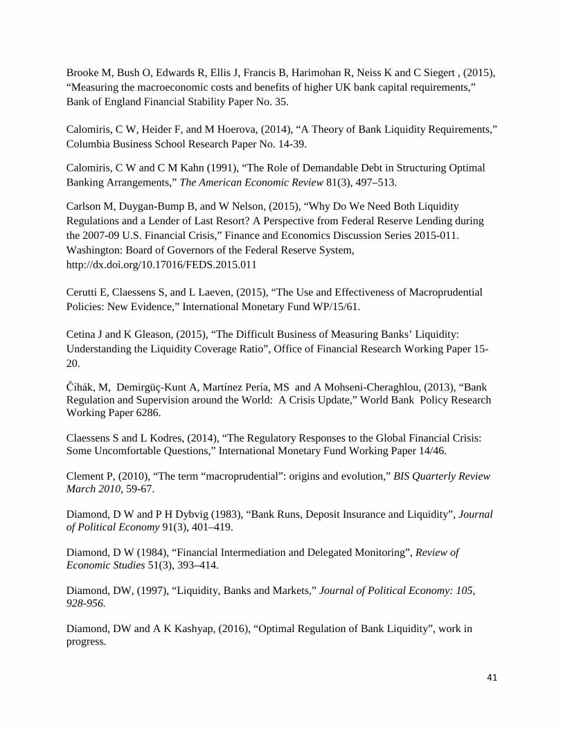
41

Brooke M, Bush O, Edwards R, Ellis J, Francis B, Harimohan R, Neiss K and C Siegert , (2015), “Measuring the macroeconomic costs and benefits of higher UK bank capital requirements,” Bank of England Financial Stability Paper No. 35.

Calomiris, C W, Heider F, and M Hoerova, (2014), “A Theory of Bank Liquidity Requirements,” Columbia Business School Research Paper No. 14-39.

Calomiris, C W and C M Kahn (1991), “The Role of Demandable Debt in Structuring Optimal Banking Arrangements,” The American Economic Review 81(3), 497–513.

Carlson M, Duygan-Bump B, and W Nelson, (2015), “Why Do We Need Both Liquidity Regulations and a Lender of Last Resort? A Perspective from Federal Reserve Lending during the 2007-09 U.S. Financial Crisis,” Finance and Economics Discussion Series 2015-011. Washington: Board of Governors of the Federal Reserve System, http://dx.doi.org/10.17016/FEDS.2015.011

Cerutti E, Claessens S, and L Laeven, (2015), “The Use and Effectiveness of Macroprudential Policies: New Evidence,” International Monetary Fund WP/15/61.

Cetina J and K Gleason, (2015), “The Difficult Business of Measuring Banks’ Liquidity: Understanding the Liquidity Coverage Ratio”, Office of Financial Research Working Paper 15-20.

Čihák, M, Demirgüç-Kunt A, Martínez Pería, MS and A Mohseni-Cheraghlou, (2013), “Bank Regulation and Supervision around the World: A Crisis Update,” World Bank Policy Research Working Paper 6286. Claessens S and L Kodres, (2014), “The Regulatory Responses to the Global Financial Crisis: Some Uncomfortable Questions,” International Monetary Fund Working Paper 14/46. Clement P, (2010), “The term “macroprudential”: origins and evolution,” BIS Quarterly Review March 2010, 59-67. Diamond, D W and P H Dybvig (1983), “Bank Runs, Deposit Insurance and Liquidity”, Journal of Political Economy 91(3), 401–419. Diamond, D W (1984), “Financial Intermediation and Delegated Monitoring”, Review of Economic Studies 51(3), 393–414. Diamond, DW, (1997), “Liquidity, Banks and Markets,” Journal of Political Economy: 105, 928-956. Diamond, DW and A K Kashyap, (2016), “Optimal Regulation of Bank Liquidity”, work in progress.

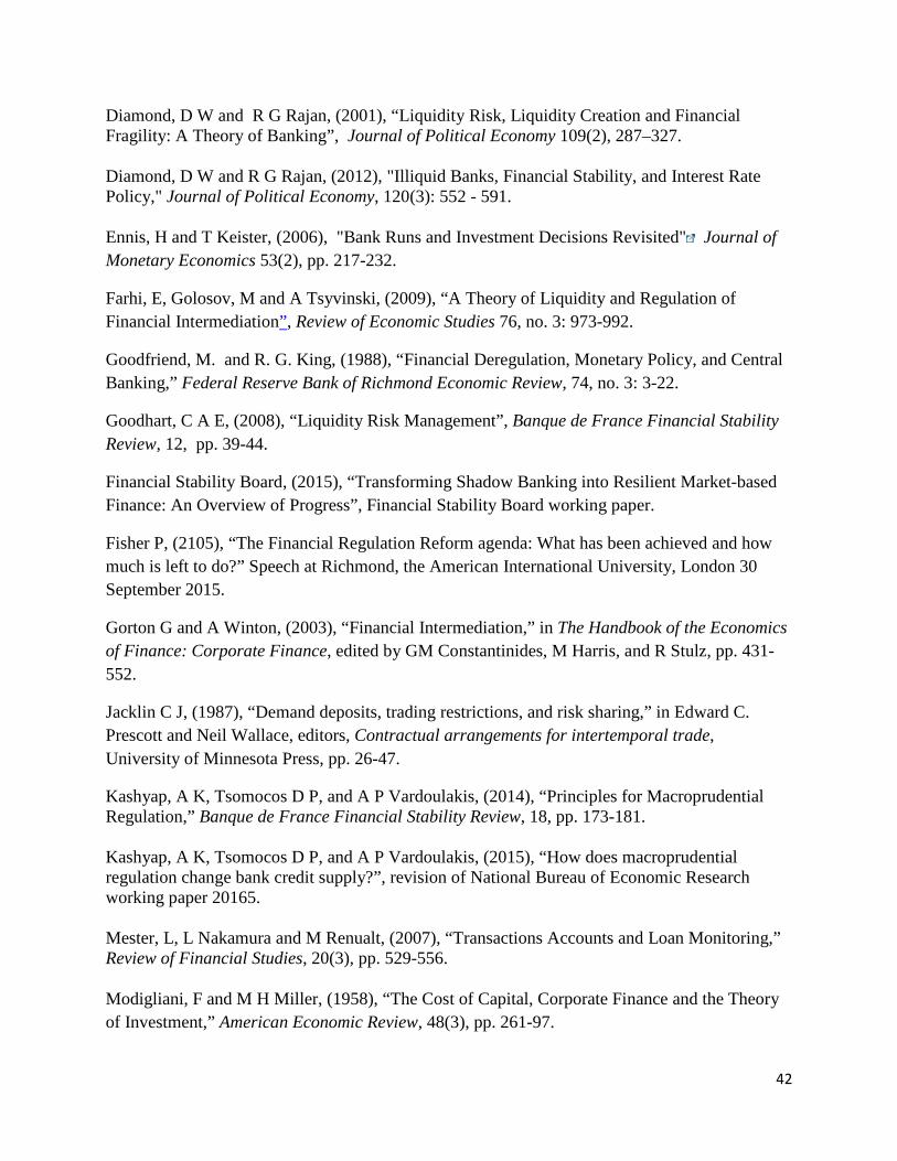
42

Diamond, D W and R G Rajan, (2001), “Liquidity Risk, Liquidity Creation and Financial Fragility: A Theory of Banking”, Journal of Political Economy 109(2), 287–327. Diamond, D W and R G Rajan, (2012), "Illiquid Banks, Financial Stability, and Interest Rate Policy," Journal of Political Economy, 120(3): 552 - 591. Ennis, H and T Keister, (2006), "Bank Runs and Investment Decisions Revisited" Journal of Monetary Economics 53(2), pp. 217-232.

Farhi, E, Golosov, M and A Tsyvinski, (2009), “A Theory of Liquidity and Regulation of Financial Intermediation”, Review of Economic Studies 76, no. 3: 973-992.

Goodfriend, M. and R. G. King, (1988), “Financial Deregulation, Monetary Policy, and Central Banking,” Federal Reserve Bank of Richmond Economic Review, 74, no. 3: 3-22.

Goodhart, C A E, (2008), “Liquidity Risk Management”, Banque de France Financial Stability Review, 12, pp. 39-44.

Financial Stability Board, (2015), “Transforming Shadow Banking into Resilient Market-based Finance: An Overview of Progress”, Financial Stability Board working paper.

Fisher P, (2105), “The Financial Regulation Reform agenda: What has been achieved and how much is left to do?” Speech at Richmond, the American International University, London 30 September 2015.

Gorton G and A Winton, (2003), “Financial Intermediation,” in The Handbook of the Economics of Finance: Corporate Finance, edited by GM Constantinides, M Harris, and R Stulz, pp. 431-552.

Jacklin C J, (1987), “Demand deposits, trading restrictions, and risk sharing,” in Edward C. Prescott and Neil Wallace, editors, Contractual arrangements for intertemporal trade, University of Minnesota Press, pp. 26-47.

Kashyap, A K, Tsomocos D P, and A P Vardoulakis, (2014), “Principles for Macroprudential Regulation,” Banque de France Financial Stability Review, 18, pp. 173-181. Kashyap, A K, Tsomocos D P, and A P Vardoulakis, (2015), “How does macroprudential regulation change bank credit supply?”, revision of National Bureau of Economic Research working paper 20165. Mester, L, L Nakamura and M Renualt, (2007), “Transactions Accounts and Loan Monitoring,” Review of Financial Studies, 20(3), pp. 529-556. Modigliani, F and M H Miller, (1958), “The Cost of Capital, Corporate Finance and the Theory of Investment,” American Economic Review, 48(3), pp. 261-97.

43

Munyan, B, (2015), “Regulatory Arbitrage in Repo Markets”, Office of Financial Research Working Paper 15-22.

Myers, S C, (1977), “Determinants of Corporate Borrowing,” Journal of Financial Economics 5, 147-175.

Norden, L and M Weber, (2010), “Credit line usage, checking account activity, and default risk of bank borrowers”, Review of Financial Studies, 23(10), pp. 3665-3699

Rochet, J C, (2014), “The extra cost of Swiss banking regulation”, Swiss Finance Institute White Paper.

Cooper, R and T W Ross, (1998), “Bank runs: Liquidity costs and investment distortions,”

Journal of Monetary Economics, 41, no. 1: 27–38.Santos, J C and J Suarez, (2015), “Liquidity standards and the value of an informed lender of last resort,” working paper, Federal Reserve Bank of New York, May.

Stein, J C, (2012), “Monetary Policy as Financial-Stability Regulation,” Quarterly Journal of Economics, 127 (1), pp. 57-95.

Uhlig, H, (2010), "A Model of a Systemic Bank Run," Journal of Monetary Economics 57, pp. 78-96.

Vives X, (2014), “Strategic Complementarity, Fragility, and Regulation”, Review of Financial Studies, 2014, 27(12), pp. 3547-3592.