The Liquidity and Liquidity Distribution Effects in Emerging Markets: The Case of

Jordan

Jérôme Vandenbussche, Szabolcs Blazsek, and Stanley Watt

WP/09/228

© 2009 International Monetary Fund WP/09/228 IMF Working Paper Monetary and Capital Markets Department

The Liquidity and Liquidity Distribution Effects in Emerging Markets: The Case of Jordan

Prepared by Jérôme Vandenbussche, Szabolcs Blazsek, and Stanley Watt1

Authorized for distribution by Daniel Hardy

October 2009

Abstract

This Working Paper should not be reported as representing the views of the IMF. The views expressed in this Working Paper are those of the author(s) and do not necessarily represent those of the IMF or IMF policy. Working Papers describe research in progress by the author(s) and are published to elicit comments and to further debate.

This paper analyzes the determinants of daily changes in Jordan’s interbank market overnight rate. It not only quantifies the classic liquidity effect, but also uncovers a liquidity distribution effect on both sides of the market, and shows that their magnitude is a decreasing and convex function of the level of excess reserves. It finds that the volatility of rate changes depends much more on the reserve surplus accumulated within a maintenance period than on the level of excess reserves. As Carpenter and Demiralp (2006), it uses the series of the central bank’s daily forecast errors to identify the liquidity effect. JEL Classification Numbers: E 43, E 52, E 58 Keywords: interbank market; liquidity effect; liquidity distribution; monetary operations

Authors’ E-Mail Addresses: jvandenbussche@imf.org; sblazsek@unav.es;

sbwatt@yahoo.com

1 The authors are affiliated to the International Monetary Fund, Universidad de Navarra, and Cornerstone Research respectively. They are very grateful to Ms. Nelly Batchoun for sharing with them the data for this paper as well as for helping interpret them, and to Daniel Hardy, Alain Ize, and Vance Martin for their useful comments on an earlier draft. This research project started when Mr. Watt was an economist at the International Monetary Fund.

2

Contents Page

I. Introduction ............................................................................................................................3

II. Literature review ...................................................................................................................6

III. The Monetary Framework and the Overnight Interbank Market in Jordan.........................8 A. The Monetary Framework and the CBJ’s Operations ..............................................8 B. The Data and a Description of the Overnight Money Market...................................9 C. Analysis of the market within a maintenance period ..............................................14

IV. Measuring the Liquidity Effect and the Liquidity Distribution Effects ............................17 A. Results of the Baseline Specification......................................................................18 B. Results of the Extended Specification.....................................................................20

V. Conclusion ..........................................................................................................................23

Tables 1. Summary Statistics.......................................................................................................13 2. Baseline Specification..................................................................................................21 3. Extended Specification (by Day of the Maintenance Period)......................................22 Figures 1. Deposits on the Overnight Window as a Ratio of Required Reserves on the Last Day

of the Maintenance Period ...........................................................................................10 2. Ratio of Excess to Required Reserves and the Interbank Rate....................................10 3. Ratio of Interbank Trading Volume to Required Reserves and the Interbank Spread to

Overnight Window Rate ..............................................................................................11 4. Window Deposit, Interbank, and Repo Rates..............................................................12 5. Interbank Window Rate Spread and Supplier Herfindahl Index .................................13 6. Interbank Window Rate Spread and Demander Herfindahl Index ..............................14 7. Interbank Spread (Over Overnight Deposit Rate) by Maintenance Day .....................17 8. Evening Ratio of Window Deposits to Required Reserves by Maintenance Day.......17 9. Ratio of Cumulative Excess Reserves (Net of Window Deposits) to Cumulative

Required Reserves by Maintenance Day .....................................................................17

3

I. INTRODUCTION

As the operational frameworks for monetary policy implementation in emerging market countries rely more and more on short-term interest rates, it is important for these countries to understand the main determinants of domestic money market rates. Accordingly, a quantitative diagnostic tool can be useful to a central bank to help interpret fluctuations in the level and volatility of short-term market rates and possibly to decide when and how much to intervene in the market, whether on a regular or an exceptional basis.2 In this paper, we perform such a quantitative analysis in the case of the Jordanian overnight interbank market over the period January 10, 2005 to March 29, 2007. As in existing studies made in the context of other countries, we discuss the existence of a liquidity effect in the overnight market—how changes in the amount of reserves in the banking system affect the overnight rate—and quantify it. In addition, we pay attention to three factors that have been previously ignored in the literature. The first is the effect of the level of daily excess reserves on the liquidity effect, and the volatility of the overnight rate. Since the typical emerging market banking system is or has historically been in a situation of time-varying excess liquidity, this factor should not be ignored. The second factor is the effect of the pattern of reserve accumulation within a reserve period on the liquidity effect and the volatility of the overnight rate. The third is the effect of changes in the distribution of daily excess reserves across banks on the overnight rate. Excess liquidity is a common feature of many emerging market banking systems and is often the result of only partial sterilization of the central bank’s accumulation of foreign assets, in particular in the case of less than fully flexible exchange rate regimes. It often also reflects the central bank’s decision to let banks hold a significant amount of precautionary excess reserves when the money market or the interbank payment system is still developing. When the level of excess liquidity in the banking system is high, banks need to rely less on the money market to satisfy their reserve requirements, and therefore the effect of a given variation in daily liquidity or daily liquidity distribution conditions can be expected to be muted. Because banks can satisfy their reserve requirements on average over the reserve maintenance period,3 the impact of a given change in daily liquidity conditions is also likely 2 Daily fluctuations in the overnight market may not be all noise. Hardy (1997) studies how a central bank should decide on the frequency with which it will conduct open market operations and the variability in short-term money market rates it will allow. He shows how the optimal operating procedure balances the value of attaining an immediate target against the value of extracting information from the free play of market forces. The contributions in Mayes and Toporowski (2007) also shed light on the issue of when, how and how much to intervene.

3 The maintenance period is the period during which banks are required to maintain reserves against their reservable deposits held during the related required reserves calculation period.

4

to depend on how far ahead or behind banks are in satisfying their reserve requirement during a given maintenance period. Similarly, the daily volatility of the overnight rate should depend on whether the banking system is advanced or is trailing in terms of satisfying the requirement. Our study focuses not only on the liquidity effect, but also on the effect of the distribution of the supply and demand for daily liquidity across banks because our dataset contains anonymous individual daily bank-by-bank data. These distribution effects have largely been ignored in the existing literature mainly because of a focus on developed economies where the interbank market is more likely to be close to perfectly competitive. By contrast, in emerging market economies with a smaller number of banks and greater market segmentation, the distribution of supply of and demand for liquidity across banks is likely to be an important factor in price formation in the money market. In the context of its currency peg to the U.S. dollar (USD), the Central Bank of Jordan (CBJ) during the period of our study typically set the level of its overnight deposit facility—which provides a floor to the overnight rate—equal to the level of the Fed Funds target, thus imposing a positive spread over the U.S. rate. However, because the CBJ did not use the overnight rate as its operating target, it typically intervened only bi-weekly in the money market through open market operations and maintained a spread of at least 250 bps between its short-term deposit and credit facilities.4 As a result, day-to-day variations of the overnight rate were much larger than in the U.S. market and largely reflected changes in local liquidity conditions. To address potential objections of endogeneity of daily changes in reserves, we follow an identification strategy similar to Carpenter and Demiralp’s (2006) and use the difference between morning projections by the CBJ and evening realizations of nonborrowed excess reserves as a highly plausibly exogenous source of variations in the daily change in nonborrowed excess reserves. Moreover, because our individual bank data are daily morning (pre-trade) projections of excess reserves for each bank, we are confident we do identify properly the effect of the distribution of excess reserves on the market rate with these data. Our variable of interest is the daily change of the spread between the overnight rate and the rate of the overnight deposit facility and we aim at understanding the determinants of its mean and variance. Our econometric model for the first difference of this spread is made of two equations considered simultaneously: (i) an ARMA(1,1)-X for the mean equation; and (ii) an EGARCH(1,1)-X for the variance equation. This type of dynamic model of mean and

4 The CBJ later introduced changes to its credit facilities in May of 2007, more than two months after the end of our sample period.

5

variance has been employed in several papers in the money market literature as discussed in the review below. Our estimates provide robust evidence that the vigor of the liquidity effect is a negative and convex function of the liquidity conditions of the day. On days when excess liquidity is scarcer, the liquidity effect gets stronger. Our dataset contains 543 observations and is therefore relatively small. Nevertheless, we also investigate the presence of a quadratic liquidity effect by day of the maintenance period and find clear evidence of a strong effect on 3 days out of the 10 in each maintenance period, in spite of the loss of identification power in that extended specification. In addition, in that same extended specification, we find weak evidence that an accumulated reserves surplus or deficit over the maintenance period has a small direct effect on the overnight rate, and stronger evidence of an additional indirect effect through its impact on the vigor of the liquidity effect. When the banking system is behind in the satisfaction of reserve requirements, the liquidity effect appears to be more powerful. Therefore, the liquidity conditions of the day and also the pattern of reserve accumulation over the maintenance period affect the determination of the overnight rate. To measure the effects of the daily distribution of liquidity across banks, we construct two normalized Herfindahl indices, one for banks with projected positive excess reserves on that day (the “suppliers”) and one for banks with negative projected excess reserves on that day (the “demanders”). We do find a statistically significant effect both for the concentration of demanders and for the concentration of suppliers. A more concentrated supply pushes the rate up, while a more concentrated demand pulls it down. As for the liquidity effect, the vigor of these distribution effects is a negative and convex function of the daily liquidity conditions, i.e., it is stronger on days when the total excess reserves of the banking system are low. Finally, our estimates for the variance equation validate our choice of an EGARCH model and indicate that the volatility of the overnight interest rate is clearly stronger when liquidity is low and especially stronger when the banking system has accumulated a reserve deficit since the start of the maintenance period The remainder of the paper is organized as follows. Section II reviews the relevant literature. Section III provides further background on the monetary framework in Jordan and contains a descriptive analysis of its overnight interbank market. Section IV presents our empirical strategy to estimate the liquidity effect and the liquidity distribution effect as well as our econometric estimates. Section V concludes.

6

II. LITERATURE REVIEW

Hamilton (1997) is the earliest paper to identify econometrically a liquidity effect at the daily frequency in the U.S. market for overnight funds. Because the level of reserves in the banking system affects the interbank rate and because the Federal Reserve also targets the interbank rate through open market operations, endogeneity of the level of reserves is a concern. Hamilton (1997) identifies the effect of exogenous liquidity shocks by constructing estimates of the forecast error of changes in the Treasury balance—the main autonomous factor of liquidity—made by the Federal Reserve trading desk. He argues that unexpected changes in the government balance provide an exogenous change to bank reserve holdings. Carpenter and Demiralp (2006) extend Hamilton’s analysis with a longer sample period and with the actual series of forecast errors made by the Federal Reserve Board—not the trading desk5—while preparing daily open market operations. They identify a liquidity effect on most days of the maintenance period. They also find that this effect is nonlinear, i.e., large changes in reserves have a more significant effect than small changes. Moreover, they find that the aggregate level of total reserve balances in the banking system also affects the magnitude of the liquidity effect. Other econometric analyses of the daily liquidity effect can be found (among others) in Thornton (2006, 2007) for the US; Bindseil and Seitz (2001), Angelini (2002), Moschitz (2004) as well as Wurtz and Krylova (2004) for the Euro Area; and Uesugi (2002) for Japan. Prati, Bartolini, and Bertola (2003) provide a comparative cross-country analysis of the overnight interbank market in G-7 countries and the Eurozone. They find that many previous models of the interbank market are not robust to changes in the institutional environment and/or style of central bank intervention. Theoretical analyses of the overnight interbank market are scarcer. One contribution of interest is Gaspar, Quirós, and Mendizábal (2004) who show how the central bank’s operational framework causes a reduction in the elasticity of the supply of funds by banks throughout the reserve maintenance period. This reduction in the elasticity together with market segmentation and heterogeneity are able to generate distributions for the interest rates and quantities traded with the same properties as in Eurozone data. To the best of our knowledge, the literature on the daily liquidity effect in emerging markets is limited to Jurgilas (2006) who studies the overnight markets of Lithuania and Bulgaria. Because these two countries operate a currency board, the central bank is prevented from

5 Thornton (2006) argues that the forecasts made by the Board (as opposed to the trading desk) are not necessarily very good ones. Because our forecasts are those made by the actual desk at the CBJ (i.e., the monetary operations department), one could argue that our instrument has greater validity than Carpenter and Demiralp’s (2006).

7

intervening in the money market through open market operations, and day-to-day fluctuations in the level of banks’ reserves solely reflect changes in autonomous factors of liquidity. In particular, because the currency board prohibits the central bank from offsetting daily fluctuations in reserves, these variations are plausibly exogenous. Using variations in the level of the Treasury account, Jurgilas (2006) does not find evidence of a daily liquidity effect in either country. However, he finds that the average deficit in reserves—the cumulative amount of closing balances below required reserves every day—is positively associated with the overnight rate in Lithuania, except for the last three days of the maintenance period. He also finds that the pattern of reserve accumulation has a significant effect on the volatility of the overnight rate in both countries. Our focus on the distribution of liquidity on the level of the overnight rate, on the effect of daily liquidity conditions on the volatility of that rate, and on the effect of the accumulation of reserves on the liquidity effect are therefore new contributions to the literature. Turning to more technical aspects, the literature has again followed the steps of the seminal paper by Hamilton (1997). He measures the instantaneous effect of an open market operation on the federal funds rate. His mean equation has an AR(p)-X structure and contains contemporaneous values of exogenous dummy variables, lagged values of interest rates and several lagged values of the endogenous variables, while his variance equation is a GARCH(1,1). The subsequent literature has typically adopted an AR(1)-X specification for the mean and an EGARCH (1,1)-X specification for the variance. Our specification is in line with the existing literature with the following exceptions. First, while previous papers have often focused on the determinants of the level of interest rates, we prefer analyzing the determinants of daily changes (i.e., the first difference), which we believe is more interesting from an operational point of view. Second, we consider a richer set of explanatory variables as discussed above, and allow the mean equation to contain a moving average term.

8

III. THE MONETARY FRAMEWORK AND THE OVERNIGHT INTERBANK MARKET IN

JORDAN

A. The Monetary Framework and the CBJ’s Operations

The Jordanian dinar (JD) has been pegged to the USD6 in a context of open capital account since 1997, which significantly limits the degree of monetary independence. As a result of a strong balance of payments since the early 2000’s, in particular sustained foreign direct investment and remittance flows, the gross usable international reserves reached the comfortable level of USD 6.1 billion (or 11 times short-term external debt at remaining maturity) as of end-December 2006. During the period of our study (January 10, 2005 to March 29, 2007), monetary operations were articulated around a system of reserve requirements (both in local and foreign currency), an overnight deposit facility, a 7-day refinancing facility7, and bi-weekly open-market operations8. The maintenance period for required reserves was 14 days, starting on Monday and ending the Sunday of the following week.9 Banks were required to maintain 65 percent of reserve requirements at all times at the central bank while the remaining 35 percent could be averaged over the maintenance period. Required reserves in local currency were 8 percent10 of daily average balances of deposits with the bank during the preceding month. Bank balances held at the CBJ (not cash in vault) were the only source of eligible reserves. Reserves requirements were set on the 5th of each month. Required reserves for the days preceding the 5th were based on the previous month’s deposit base while requirements after the 5th were based on the new deposit base. The period of study was one of financial stability and sustained economic growth both in Jordan and in the United States. During that period , the rate of the overnight deposit facility was consistently adjusted on the Sunday following a change in the U.S. Fed funds’ target rate. The rate of the refinancing facility was 250 bps above that of the overnight deposit facility before October 9, 2005, and 300 bps thereafter. The CBJ’s open market operations took the form of an auction of central bills with maturities of 3 months and 6 months

6 Since October 1995, the Dinar has been officially pegged to the SDR but in practice has been pegged to the USD. The parity is fixed at 0.709 Jordanian Dinar per USD and there is a band of +/- 0.15 percent around the central parity.

7 In May of 2007, the maturity of that facility was reduced to overnight.

8 On very rare occasions, the CBJ intervened once in-between two auctions.

9 The week-end is Friday and Saturday in Jordan.

10 These rules for reserve requirements were in place since September 6, 2004.

9

typically on the second Wednesday of each maintenance period.11 Settlement proceeded two working days later, typically the following Sunday. Finally, the CBJ stood ready to buy or sell any amount in foreign exchange based on their bid/ask quotes published daily. Our analysis focuses on all banks operating in Jordan at the time with the exclusion of the two Islamic banks, which did not participate in the money market, did not deposit funds on the overnight facility and did not take part in auctions of central bank bills or government securities. Therefore, for our purposes, the banking sector consisted of 21 banks, all private.12 The banking system was usually characterized as concentrated, with the top three banks having a combined market share over 40 percent as of end-2006.

B. The Data and a Description of the Overnight Money Market

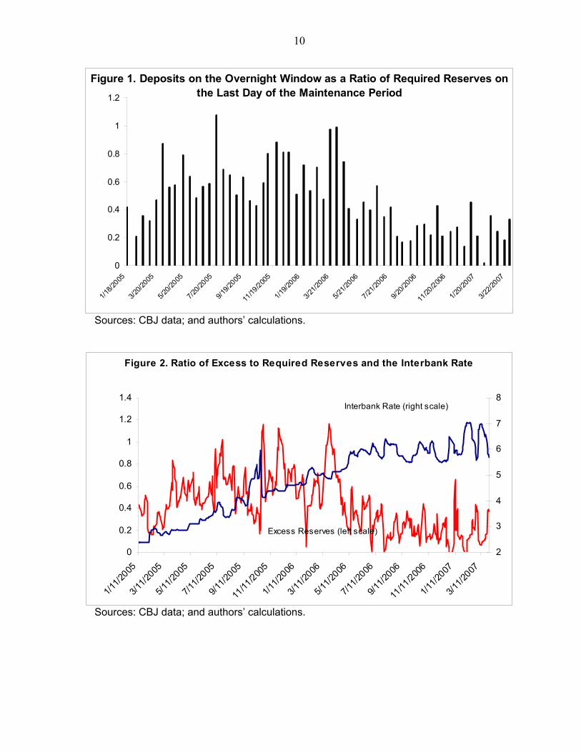
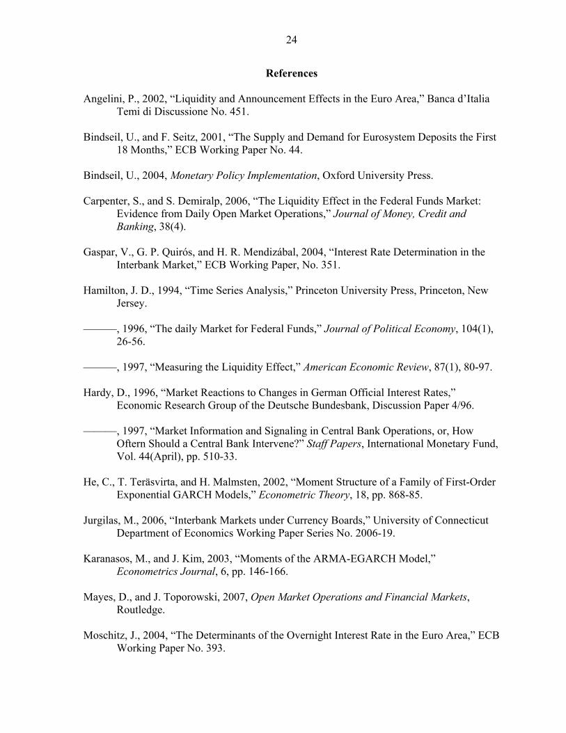
The data covers the period January 10, 2005 to March 29, 2007. For the aggregate banking system, we have daily data on the interbank overnight interest rate, the volume of transactions, the rates of the two CBJ facilities, and the end-of-the-day reserves position. For each individual bank,13 we have the amount of deposits on the overnight deposit window, the amount of borrowings from the refinancing window, required reserves, and a morning projection of evening reserves made by the CBJ’s monetary operations department. During the period of study, the banking system in Jordan was generally in a situation of excess liquidity, as the total banking system held large deposits on the overnight window on the last day of each maintenance period (Figure 1). While until mid-2006, excess liquidity represented about fifty percent of required reserves, it dropped by half on average in the most recent period as the CBJ sought to rein in an acceleration in private sector credit growth. In parallel, the daily volatility of excess reserves also declined somewhat after mid-2006 but variations in excess reserves looked more closely associated with movements in the overnight rate (Figure 2). Interbank trading volume also increased over the sample period, in connection with the decline in excess liquidity (Figure 3).

11 In a few instances, auctions took place during the first week of the maintenance period.

12 The banking system as a whole had JD 24.2 billion of assets, or 240 percent of GDP, and was well capitalized by international standards as of end-2006.

13 These data are completely anonymous.

10

Sources: CBJ data; and authors’ calculations.

Sources: CBJ data; and authors’ calculations.

0

0.2

0.4

0.6

0.8

1

1.2

1/18

/2005

3/20

/2005

5/20

/2005

7/20

/2005

9/19

/2005

11/19

/200

5

1/19

/2006

3/21

/2006

5/21

/2006

7/21

/2006

9/20

/2006

11/20

/200

6

1/20

/2007

3/22

/2007

Figure 1. Deposits on the Overnight Window as a Ratio of Required Reserves onthe Last Day of the Maintenance Period

0

0.2

0.4

0.6

0.8

1

1.2

1.4

1/11

/2005

3/11

/2005

5/11

/2005

7/11

/2005

9/11

/2005

11/11

/200

5

1/11

/2006

3/11

/2006

5/11

/2006

7/11

/2006

9/11

/2006

11/11

/200

6

1/11

/2007

3/11

/2007

2

3

4

5

6

7

8

Figure 2. Ratio of Excess to Required Reserves and the Interbank Rate

Excess Reserves (left scale)

Interbank Rate (right scale)

11

Sources: CBJ data; and authors’ calculations. In spite of this situation of excess liquidity, the spread between the interbank rate and the rate of the overnight deposit window remained strictly positive, ranging between 12 and 192 bps (see Figures 3 and 4)14. This is suggestive of market imperfections and justifies our focus on the effect of the distribution of liquidity on the determination of the interbank rate. In addition, on a few episodes early in the sample period, the market rate did not fully adjust to changes in the U.S. rate the day following a Fed announcement (typically a Wednesday), although banks could anticipate that the CBJ would follow suit the following Sunday. This suggests a lack of full arbitrage across days within a maintenance period. Evidence of incomplete arbitrage is also clear from the spike in the interest rate on October 19-20, 2005 followed by a drop of 170 bps on October 21, the 7th day of the maintenance period and a day when a large amount of central bank bills matured, an injection of liquidity which would have been expected by market participants.15

14 Of course a positive interbank spread could also coexist with sizeable surplus liquidity if banks’ end-of-the-day (i.e., post interbank market) reserves position is volatile, reflecting the nature of the payments system.

15 It is likely that the requirement to hold at least 65 percent of required reserves each day (i.e., less-than-full averaging) played a role during that episode.

0

0.1

0.2

0.3

0.4

1/11

/2005

3/11

/2005

5/11

/2005

7/11

/2005

9/11

/2005

11/11

/200

5

1/11

/2006

3/11

/2006

5/11

/2006

7/11

/2006

9/11

/2006

11/11

/200

6

1/11

/2007

3/11

/2007

0

0.5

1

1.5

2

2.5

Figure 3. Ratio of Interbank Trading Volume to Required Reserves and the Interbank Spread to Overnight Window Rate

Interbank Trading Volume (left scale)

Interbank Spread (right scale)

12

Sources: CBJ data; and authors’ calculations.

To gauge distribution effects, we construct two normalized Herfindahl indices based on morning (and therefore pre-interbank trade) projections of bank-by-bank excess liquidity. A Herfindahl index is constructed for banks with projected reserves exceeding their required reserves on the day (“suppliers”) and one for banks with projected reserves below their required reserves for the day (“demanders”). We acknowledge that this is an imperfect way to capture the supply and demand for liquidity, as a bank’s behavior depends not only on its liquidity position at one point in time, but also on the average reserves it has accumulated on previous days of the maintenance period and its forecast of its future reserve holdings until the end of the maintenance period. Table 1 presents summary statistics of our main variables of interest.

Figure 5 and 6 show the evolution over time of the distribution of excess reserves as well as of that of reserve deficits as measured by the two indices. While fluctuations around the mean of each series are typically small, one observes occasional spikes of concentration on both sides of the market. Moreover, variations of the supplier index appear to be larger in the second half of the sample period, at a time when aggregate excess liquidity was generally lower, which should help the identification.

2

3

4

5

6

7

8

9

1/10

/2005

3/12

/2005

5/12

/2005

7/12

/2005

9/11

/2005

11/11

/200

5

1/11

/2006

3/13

/2006

5/13

/2006

7/13

/2006

9/12

/2006

11/12

/200

6

1/12

/2007

3/14

/2007

Figure 4. Window Deposit, Interbank, and Repo Rates

Repo Rate

Window Deposit Rate

Interbank Rate

13

Table 1. Summary Statistics Observations Mean Std Dev Min Max Interbank Rate 543 4.78 1.26 2.38 7.04Window Rate 543 4.30 1.03 2.25 5.25Interbank Spread 543 0.48 0.39 0.12 1.95∆(Interbank Spread) 543 0.00 0.11 -1.70 0.60Required Reserves (JD Millions) 543 485.8 76.8 381.3 644.9Excess Reserves (JD Millions) 543 199.2 114.1 -69.2 542.1Excess to Required Reserves 543 0.43 0.26 -0.11 1.16∆(Excess to Required Reserves) 543 0.00 0.10 -0.46 0.88Interbank Volume to Required Reserves 543 0.16 0.07 0.02 0.37Window Deposits to Required Reserves 543 0.41 0.25 0.00 1.20Repo Borrowings to Required Reserves 543 0.00 0.02 0.00 0.17Cumulative Sum 543 0.05 0.04 -0.03 0.21Herfindahl Supplier 543 0.13 0.06 0.04 0.60Herfindahl Demander 543 0.09 0.07 0.01 0.74

Sources: CBJ data and authors calculations.

Sources: CBJ data; and authors’ calculations.

0

0.5

1.0

1.5

2.0

2.5

1/11

/2005

3/11

/2005

5/11

/2005

7/11

/2005

9/11

/2005

11/11

/200

5

1/11

/2006

3/11

/2006

5/11

/2006

7/11

/2006

9/11

/2006

11/11

/200

6

1/11

/2007

3/11

/2007

0.06

0.16

0.26

0.36

0.46

0.56

0.66

Figure 5. Interbank Window Rate Spread and Supplier Herfindahl Index

Interbank Spread (left scale)

Herfindahl Index (right scale)

14

Sources: CBJ data; and authors’ calculations.

C. Analysis of the market within a maintenance period

We next turn to examining the behavior of some of our main variables of interest within the maintenance period. With rational expectations, the overnight rate should theoretically be a martingale, as only unexpected shocks should affect the interbank rate (see chapter 3 in Bindseil (2004)).16 Hamilton’s (1996) econometric study of the U.S. federal funds rate questioned the empirical validity of the martingale hypothesis, suggesting that banks in fact do not regard reserves held on different days of the week as perfect substitutes. In the Jordanian data, although the interbank rate seems to peak near the end of the first week of the maintenance period, the difference across days is small (Figure 7). Thus, at first glance, we do not seem to find evidence contradicting a martingale hypothesis. Nevertheless, episodes such as that of October 19-21, 2005 described above indicate that arbitrage is sometimes far from perfect.

16 In probability theory, a martingale is a stochastic process in which the conditional expectation of the next value, given the current and preceding values, is the current value. If the martingale property holds, predictable changes in reserves should not cause predictable changes in interest rates within reserve maintenance periods.

0

0.5

1.0

1.5

2.0

2.5

1/11

/2005

3/11

/2005

5/11

/2005

7/11

/2005

9/11

/2005

11/11

/200

5

1/11

/2006

3/11

/2006

5/11

/2006

7/11

/2006

9/11

/2006

11/11

/200

6

1/11

/2007

3/11

/2007

0.06

0.16

0.26

0.36

0.46

0.56

0.66

Figure 6. Interbank Window Rate Spread and Demander Herfindahl Index

Interbank Spread (left scale)

Herfindahl Index (right scale)

15

Looking next at the amount banks deposit at the central bank overnight window by day of the maintenance period, it appears that as the maintenance period progresses, banks tend to deposit larger and larger amounts at the overnight window (Figure 8). This is consistent with a system with generally a surplus in reserves. Banks try to satisfy their reserve requirements early in the period as insurance against a possible future negative shock. Since the system tends to end in surplus, as the maintenance period progresses, banks deposit their excess liquidity at the interest bearing facility at the central bank. This behavior may explain why overnight rates appear marginally higher during the first week of the maintenance period. Analogously, the ratio of cumulative excess reserves to cumulative required reserves over the maintenance period falls as the period progresses (Figure 9). Again, in a system with general surplus liquidity, banks develop a buffer for their reserve requirements early in the maintenance period and draw down their buffer with the overnight window as the period progresses.

IV. MEASURING THE LIQUIDITY EFFECT AND THE LIQUIDITY DISTRIBUTION EFFECTS

We next move on to measure the liquidity effect in the overnight interbank market by examining the relationship between the daily change in the banking system’s excess reserves and the daily change in the interbank overnight rate. More precisely, our dependent variable is the first difference of the spread between the interbank rate and the deposit window rate, as the overnight window rate (set by the CBJ) is the guaranteed rate than any bank would be able to attain. Our measure of liquidity is the level of non-borrowed excess reserves in the banking system (defined as the evening closing balance of the system minus required reserves plus the amount held at the overnight window net of any repo borrowings outstanding) which we normalize by dividing by the amount of required reserves. Estimating the relationship in first differences has three advantages. First, it allows us to obtain estimates that are more useful from an operational perspective. Second, interest rates, especially at short horizons, are often close to unit root processes and we cannot reject the null of a unit root in levels in the data. Third, as described further below, a series of plausibly exogenous shocks to the daily change in excess reserves is available. Because of the averaging system, the amount of excess liquidity on any given day does not fully capture overall liquidity conditions. A day with large amounts of excess reserves but which also finds banks behind in their reserve accumulation is different from a day with an equal amount of aggregate excess reserves but where banks are well ahead in satisfying their reserve requirement. To control for these differences, we also include as an explanatory variable a cumulative sum variable which is defined as the cumulative sum of the closing balance minus required reserves of the whole system since the first day of the maintenance period normalized by the cumulative sum of required reserves since the first day of the maintenance period.

16

Sources: CBJ data; and authors’ calculations.

Sources: CBJ data; and authors’ calculations.

Sources: CBJ data; and authors’ calculations.

0.30

0.35

0.40

0.45

0.50

1 2 3 4 7 8 9 10 11 14

Figure 7. Interbank Spread (over Overnight Deposit Rate) by Maintenance Day

0.30

0.35

0.40

0.45

0.50

1 2 3 4 7 8 9 10 11 14

Figure 8. Evening Ratio of Window Deposits to Required Reserves by Maintenance Day

0.000

0.015

0.030

0.045

0.060

0.075

0.090

1 2 3 4 7 8 9 10 11 14

Figure 9. Ratio of Cumulative Excess Reserves (Net of Window Deposits) to Cumulative Required Reserves by Maintenance Day

17

As already mentioned above, to measure the impact of the distribution of liquidity among banks on the overnight rate we compute normalized Herfindahl indices for banks that have positive excess reserves and for banks that have negative excess reserves. This gives us a sense of the concentration and potential market power of banks that are suppliers or demanders on the interbank market. Although we have good reasons to expect to find a liquidity effect and distribution effects, the strength of these effects should presumably be contingent on general liquidity conditions. In fact, casual inspection of Figure 2 suggests that the liquidity effect is more prevalent on days when excess reserves are low. We test this hypothesis by including various interaction terms. We interact the change in the aggregate liquidity level and changes in liquidity distribution both with the level of liquidity and its square (to capture possible non-linearities), and also interact our cumulative sum variable with the change in the liquidity level. We include dummies for each day of the maintenance period, the beginning and end of each month, the beginning and end of each quarter, the day before and after a holiday, and the day of and days surrounding a change in the overnight window rate, to account for possible shifts in the demand for reserves on these special days. As in the existing literature, we are also interested in modeling the volatility of our dependent variable. Our error process is thus assumed to display autoregressive conditional heteroskecasticity. Specifically, we employ an EGARCH model that allows the effect of yesterday’s error term on today’s error term to differ depending on whether the shock was positive or negative and allows explanatory variables of the variance equation to have a negative sign. We conjecture that the volatility of our dependent variable is determined by the liquidity conditions of the day, our cumulative sum variable and a subset of the dummies included in the mean equation. Days when liquidity conditions are tighter should witness higher volatility. For the whole banking system, once reserve requirements are set, we know that reserve holdings between two regular open market operations are essentially exogenous as their variation depends only on that of the autonomous factors of liquidity. Yet, to address concerns about the potential endogeneity of day-to-day changes in the supply of reserves, we focus our analysis on the effect of the unexpected component of the day-to-day changes in reserves. To do so, we construct the series of the forecast error made by the CBJ in its daily morning liquidity forecasting exercise17 and use this forecast error (normalized by required reserves) as our key variable to identify the liquidity effect in equation (1) below. This forecast error series is a valid source of exogenous shocks because the CBJ can arguably

17 This is the difference between actual evening closing balances and CBJ morning projections of the closing balances.

18

anticipate and forecast high-frequency variations in autonomous factors of liquidity much better than market participants. After trying specifications with various lag and MA structures, we finally decided to include one lag of the dependent variable and to allow the error term of our mean equation to be MA(1). Our model is thus ARMA(1,1)-EGARCH(1,1)-X and can be written as follows:

(Δs)t = φ (Δs)t-1 + m·Xt + εt + ψ εt-1 (1) __ ___

log ht = ω + β log ht-1 + ν·Yt + α | ε t-1 / √ ht-1 | + γ ε t-1 / √ ht-1 (2) __

ε t = √ht ut (3) where (Δs) is the daily change in the spread between the market rate and the rate of the deposit facility, ut ~ N(0,1) is an i.i.d. error term, m and ν are vectors of real parameters and φ, ψ, ω, β, α, γ are scalars. The Xt and Yt vectors denote the explanatory variables in the mean and variance equations respectively. In our empirical application, we shall consider two different sets of Xt and Yt variables. Therefore, we shall be more specific regarding these components later. One advantage of the EGARCH formulation for log volatility is that there are no sign restrictions for the v parameters of the explanatory variables. The φ and β parameters capture AR(1) and GARCH(1) dynamics, while the ψ and α parameters measure the MA(1) and ARCH(1) dynamics. As discussed in He et al. (2002) and Karanasos and Kim (2003),18 the stationarity of the ARMA(1,1)-EGARCH(1,1)-X model is provided by the following two conditions: (1) | φ | < 1; and (2) | β | < 1. These conditions turn out to be satisfied in the three specifications we discuss below. Finally, the γ parameter introduces the possibility of asymmetry into the volatility equation.

A. Results of the Baseline Specification

The upper part of Table 2 provides our estimates for the mean equation while the lower part presents the results for the variance equation. The X vector includes the CBJ’s forecast error (“Shock”), its interactions with the level of excess reserves (RER) and its square, its interaction with the level of accumulated reserves since the beginning of the reserve period (“cumulative sum”), the first difference of that cumulative sum variable, the first difference of our Herfindahl index for liquidity suppliers (“herf suppliers”) and its interactions with the level of excess reserves and its square, the first difference of our Herfindahl index for liquidity demanders (“herf demanders”) and its interactions with the level of excess reserves and its square, and our full set of dummy variables. The Y vector includes the level of excess reserves, the level of accumulated reserves since the beginning of the reserve period and our

18 These authors build on Hamilton (1994); and Nelson (1991).

19

set of dummy variables excluding dummies for days of the maintenance period which all turn out to be econometrically insignificant. Liquidity effect We do find robust evidence of a liquidity effect, the strength of which is a negative and convex function of the level of excess reserves on that day. In this baseline specification, the accumulation of reserves since the beginning of the reserve period does not seem to affect the day-to-day changes in interest rate, either directly or through its impact on the liquidity effect but this more encouraging results appear when we look at the extended specification below. A positive supply shock to bank reserves representing 26 percent of required reserves (i.e., the equivalent of one standard deviation of that variable) would decrease the spread by about 10 bps when the level of the excess to required reserves ratio is close to minimum sample value, but would not move when liquidity conditions are loose. Of course, these effects represent only the impact on the day of the shock. The first-order auto-correlation coefficient of 0.62 implies an additional effect on the second and third day as well. Distribution effects We also find strong evidence of econometrically significant distribution effects on both sides of the market which are also contingent on the level of daily excess reserves. As for the liquidity effect, the relationship is negative and convex (in both cases, the quadratic term is at the border of conventional levels of significance). The effect on the supply side is about twice as strong as that on the demand side. Days where excess liquidity becomes more concentrated experience an increase in interbank interest rates, especially when the level of excess reserves is low. A positive one-standard-deviation shock to our Herfindahl index for suppliers (resp. demanders) increases (resp. decrease) the spread by about 4 bps (resp. 2 bps) when the excess to required reserves is at the sample minimum, but has no impact when there is ample liquidity. Nevertheless, a sudden shift in the distribution of excess reserves which would bring the one of our Herfindahl indices from the sample mean to its maximum sample value would impact the spread by 20 to 25 basis points on the same day if the level of excess reserves is low. Special day effects In our regression, only one maintenance day dummy (for day 8) is significant but the effect is small. We do not observe any special end-of-the-month or holiday effect either. Interestingly, not adjusting for the effect of its lagged changes, the spread declines by 12 bps on days where the policy rate (i.e. the rate of the overnight deposit facility) is adjusted and climbs by 5 bps the day before and 5 bps the day after. As can be seen in Figure 4, the policy rate was only adjusted upward during our sample period, typically with a three day lag after a change in the U.S. Fed Funds rate, and our estimates indicate that the adjustment of the spread to the

20

new policy rate is gradual over three business days. This finding of a run-up to the day of the policy decision echoes the work of Hardy (1996) who analyzes the reaction of market interest rates to both anticipated and unanticipated components of changes in the Bundesbank’s official policy rates. Volatility and excess reserves Results for the variance equation clearly show that a higher level of excess reserves decreases the volatility of the spread, as expected. Perhaps more interestingly, they also indicate that the sum of accumulated reserves above the required amount has an even stronger volatility-reducing effect. Our estimates also indicate the presence of bouts of volatility at the end of the month and after a holiday, probably because of increased payment activity and sudden shifts in the demand for reserves on those days. Changes in policy rates are associated with more volatility beforehand as the market shows signs of small tension in the run-up to the day of a policy decision, and less volatility once the announced policy change has actually been implemented and potential uncertainty surrounding policy changes has vanished.

B. Results of the Extended Specification

We also analyze the liquidity effect by day within the maintenance period as previous authors have done. We take our baseline specification and systematically replace the forecast error (whether interacted or not) by the forecast error multiplied by each of the 10 day dummies. As discussed above, this specification is very demanding given the relatively short dataset we have (543 observations). Results presented in Table 3 indicate that a highly significant liquidity effect can be observed on days 4, 7, and 11 of the maintenance period and is particularly strong on day 7 when liquidity in the banking system is scarce. The effect observed on days 4 and 11 possibly reflects the fact that reserves deposited at the central bank on a day before the two-day week-end actually count three times toward the satisfaction of reserve requirements, which makes reserves relatively more valuable on those days. We do not find an econometrically significant liquidity effect on the last day of the maintenance period, perhaps reflecting the fact that reserve requirements are already almost fully met by the end of day 13. Both distribution effects are again present. The effect on the supply side is of the same magnitude as before, while that on the demand side is stronger and significantly convex. Interestingly, the effect of the reserve accumulation pattern since the beginning of the reserve period on the liquidity effect is now significant and strong. Estimates for dummy variables and the variance equation are largely similar to those obtained under the baseline.

21

Dependent Variable: First Difference of Spread (∆s)t

Mean EquationCoefficient St.dev. p-value

(∆s)t-1 0.62 *** 0.05 0.00Shock -0.33 *** 0.05 0.00Shock*RER 0.91 *** 0.21 0.00Shock*(RER)² -0.65 *** 0.22 0.00Shock*Cumulative Sum 0.05 0.60 0.93∆(Cumulative Sum) -0.02 0.05 0.73∆(Herf. Suppliers) 0.52 *** 0.13 0.00∆(Herf Suppliers) * RER -1.10 ** 0.48 0.02∆(Herf Suppliers) * (RER)² 0.62 0.41 0.13∆(Herf. Demanders) -0.27 ** 0.13 0.04∆(Herf. Demanders) * RER 0.65 * 0.37 0.08∆(Herf. Demanders) * (RER)² -0.39 0.25 0.12Dummy day1 0.00 0.00 0.47Dummy day2 0.01 0.01 0.19Dummy day3 0.00 0.00 0.67Dummy day4 0.00 0.00 0.41Dummy day7 0.00 0.01 0.95Dummy day8 -0.01 * 0.00 0.09Dummy day9 0.00 0.00 0.64Dummy day10 0.00 0.00 0.24Dummy day11 0.00 0.00 0.56Dummy day14 0.00 0.01 0.69Dummy end-of-month 0.00 0.01 0.46Dummy start-of-month 0.00 0.01 0.50Dummy (holiday + 1) 0.00 0.01 0.59Dummy (holiday - 1) 0.00 0.00 0.56Dummy (policy change + 1) 0.05 *** 0.01 0.00Dummy policy change -0.12 *** 0.02 0.00Dummy (policy change - 1) 0.05 *** 0.01 0.00MA(1) -0.31 *** 0.07 0.00

Variance EquationCoefficient St.dev. p-value

Constant -1.33 *** 0.10 0.00Alpha: ARCH(1) 0.96 *** 0.07 0.00Gamma: Asymmetry parameter 0.31 *** 0.05 0.00Beta: GARCH(1) 0.87 *** 0.02 0.00Excess Reserves -0.81 *** 0.09 0.00Cumulative Sum -4.43 *** 0.97 0.00Dummy end-of-month 1.39 *** 0.34 0.00Dummy start-of-month -0.36 0.32 0.26Dummy (holiday + 1) 2.35 *** 0.15 0.00Dummy (holiday - 1) -0.47 *** 0.14 0.00Dummy (policy change + 1) -2.18 *** 0.71 0.00Dummy policy change -1.07 0.84 0.20Dummy (policy change - 1) 2.27 *** 0.71 0.00

Regression Summary Statistics

R-squared 0.13Adjusted R-squared 0.08S.E. of regression 0.11Sum squared resid 6.07Log likelihood 963.57Akaike info criterion -3.40Schwarz criterion -3.06Durbin-Watson stat 1.89

Sources: CBJ data; and authors calculations.Note: three, two, and one star indicate significance at the 1, 5 and 10 percent levelrespectively. RER is the ratio of excess to required reserves."Shock" is the forecast error.

Table 2. Baseline Specification

22

Dependent Variable: First Difference of Spread (∆s)t

Mean EquationCoefficient St.dev. p-value Coefficient St.dev. p-value

(∆s)t-1 0.39 *** 0.05 0.00 Dummy day1 -0.01 0.01 0.24

Shock*Dummy day 1 1.10 0.93 0.24 Dummy day2 0.02 ** 0.01 0.01Shock*Dummy day 2 1.41 0.94 0.13 Dummy day3 0.01 ** 0.00 0.01Shock*Dummy day 3 -0.46 0.49 0.35 Dummy day4 0.00 0.01 0.91Shock*Dummy day 4 -0.86 *** 0.30 0.00 Dummy day7 0.01 0.01 0.65Shock*Dummy day 7 -2.14 *** 0.44 0.00 Dummy day8 -0.01 *** 0.00 0.00Shock*Dummy day 8 -0.12 0.30 0.69 Dummy day9 0.00 0.00 0.87Shock*Dummy day 9 -0.30 0.73 0.68 Dummy day10 0.00 0.00 0.64Shock*Dummy day 10 0.25 0.26 0.34 Dummy day11 0.00 0.01 0.53Shock*Dummy day 11 -0.56 *** 0.16 0.00 Dummy day14 -0.01 0.01 0.47Shock*Dummy day 14 -1.47 0.96 0.13 Dummy end-of-month -0.01 0.01 0.42Shock*RER*Dummy day 1 -7.94 * 4.73 0.09 Dummy start-of-month 0.01 ** 0.00 0.04Shock*RER*Dummy day 2 -5.47 3.47 0.12 Dummy (holiday + 1) 0.00 0.01 0.68Shock*RER*Dummy day 3 -0.21 1.84 0.91 Dummy (holiday - 1) 0.00 0.01 0.47Shock*RER*Dummy day 4 1.23 0.98 0.21 Dummy (policy change + 1) 0.05 *** 0.01 0.00Shock*RER*Dummy day 7 6.37 *** 1.46 0.00 Dummy policy change -0.11 *** 0.02 0.00Shock*RER*Dummy day 8 2.48 ** 1.14 0.03 Dummy (policy change - 1) 0.05 *** 0.01 0.00Shock*RER*Dummy day 9 0.33 3.03 0.91 MA(1) 0.06 0.06 0.35Shock*RER*Dummy day 10 -2.32 * 1.35 0.09Shock*RER*Dummy day 11 0.45 0.70 0.52 Variance EquationShock*RER*Dummy day 14 5.79 * 3.29 0.08 Coefficient St.dev. p-valueShock*(RER)²*Dummy day 1 9.59 * 5.27 0.07 Constant -1.87 *** 0.14 0.00Shock*(RER)²*Dummy day 2 3.40 3.13 0.28 Alpha: ARCH(1) 1.10 *** 0.10 0.00Shock*(RER)²*Dummy day 3 0.26 1.41 0.85 Gamma: Asymmetry paramet 0.34 *** 0.06 0.00Shock*(RER)²*Dummy day 4 -1.29 * 0.72 0.07 Beta: GARCH(1) 0.78 *** 0.02 0.00Shock*(RER)²*Dummy day 7 -4.73 *** 1.16 0.00 Excess Reserves -0.98 *** 0.14 0.00Shock*(RER)²*Dummy day 8 -4.77 *** 1.06 0.00 Cumulative Sum -4.95 *** 1.38 0.00Shock*(RER)²*Dummy day 9 -0.57 2.72 0.83 Dummy end-of-month 0.54 0.34 0.12Shock*(RER)²*Dummy day 10 2.39 * 1.38 0.08 Dummy start-of-month -0.28 0.32 0.38Shock*(RER)²*Dummy day 11 0.08 0.74 0.91 Dummy (holiday + 1) 2.38 *** 0.17 0.00Shock*(RER)²*Dummy day 14 -6.47 ** 2.88 0.02 Dummy (holiday - 1) -0.54 *** 0.18 0.00Shock * (Cumulative Sum) 6.13 *** 1.71 0.00 Dummy (policy change + 1) -1.07 0.85 0.21∆(Cumulative Sum) -0.10 0.07 0.12 Dummy policy change -1.34 * 0.70 0.06∆(Herf. Suppliers) 0.53 *** 0.14 0.00 Dummy (policy change - 1) 1.89 ** 0.79 0.02∆(Herf Suppliers) * RER -1.27 ** 0.60 0.04∆(Herf Suppliers) *(RER)² 0.77 0.55 0.16 Regression Summary Statistics∆(Herf. Demanders) -0.41 ** 0.17 0.01∆(Herf. Demanders) * RER 1.13 ** 0.47 0.02 R-squared 0.15∆(Herf. Demanders) *(RER)² -0.74 ** 0.32 0.02 Adjusted R-squared 0.05

S.E. of regression 0.11Sum squared resid 5.92Log likelihood 937.82Akaike info criterion -3.21Schwarz criterion -2.65Durbin-Watson stat 2.25

Sources: CBJ data; and authors calculations

Note: three, two, and one star indicate significance at the 1, 5 and 10 percent level respectively."Shock" is the forecast error. RER is the ratio of excess to required reserves.

Table 3. Extended Specification (by Day of the Maintenance Period)

23

V. CONCLUSION

Using daily Jordanian data, we perform a comprehensive econometric study of the overnight interbank market. We find a robust negative relationship between daily changes in the amount of excess reserves and daily changes in the spread between the interbank rate and the rate of the overnight deposit facility. We find strong evidence that this effect is much more powerful when excess reserves on a given day are low and some evidence that it is also more vigorous when banks have accumulated a reserve deficit since the beginning of the maintenance period. On a day with tight liquidity conditions and where the banking system has no surplus in accumulated reserves, our estimates suggest that a supply shock equivalent to 26 percent of required reserves would affect the spread by about 10 basis points on the day of the shock, with smaller additional impacts over the next 1-2 days because of the auto-regressive pattern of the first difference in the spread. Using anonymous individual bank data, we are able to calculate Herfindahl indices for both potential demanders and suppliers of reserves in the interbank market. We find evidence for distribution effects on both sides of the market. As for the level of reserves, the effect of the distribution of excess reserves is a decreasing and convex function of the level of excess reserves and thus we estimate much stronger effects when liquidity conditions are tight. A shock of one standard deviation to our suppliers (resp. demanders) index would barely move the rate under average liquidity conditions and would move it by 3 to 4 (resp. 2 to 3) basis points on the day of the shock under tight liquidity conditions. Our econometric estimates were obtained in the context of a specific operational framework for monetary policy implementation and there is no guarantee that they would be perfectly robust to a change in this framework and/or procedures. Nevertheless, we believe our approach is general enough that it could easily be adjusted or replicated under a different framework and also therefore in the context of other emerging market countries. To the extent that this approach has successfully identified truly exogenous shocks to the supply of bank reserves, it makes it possible to deliver a quantitative assessment of the control that a central bank can exert on the interbank overnight rate through regular or exceptional open market operations. Changes in the distribution of excess reserves are largely out of the day-to-day control of a central bank, but our analysis has provided both an easy-to-compute indicator to monitor daily the evolution of the distribution of excess reserves in the banking system and a practical way to measure its impact in the market for reserves and, therefore, to assess how to neutralize it through monetary operations if so desired.

24

References

Angelini, P., 2002, “Liquidity and Announcement Effects in the Euro Area,” Banca d’Italia Temi di Discussione No. 451. Bindseil, U., and F. Seitz, 2001, “The Supply and Demand for Eurosystem Deposits the First 18 Months,” ECB Working Paper No. 44. Bindseil, U., 2004, Monetary Policy Implementation, Oxford University Press. Carpenter, S., and S. Demiralp, 2006, “The Liquidity Effect in the Federal Funds Market:

Evidence from Daily Open Market Operations,” Journal of Money, Credit and Banking, 38(4).

Gaspar, V., G. P. Quirós, and H. R. Mendizábal, 2004, “Interest Rate Determination in the Interbank Market,” ECB Working Paper, No. 351. Hamilton, J. D., 1994, “Time Series Analysis,” Princeton University Press, Princeton, New

Jersey. ———, 1996, “The daily Market for Federal Funds,” Journal of Political Economy, 104(1), 26-56. ———, 1997, “Measuring the Liquidity Effect,” American Economic Review, 87(1), 80-97. Hardy, D., 1996, “Market Reactions to Changes in German Official Interest Rates,”

Economic Research Group of the Deutsche Bundesbank, Discussion Paper 4/96. ———, 1997, “Market Information and Signaling in Central Bank Operations, or, How

Oftern Should a Central Bank Intervene?” Staff Papers, International Monetary Fund, Vol. 44(April), pp. 510-33.

He, C., T. Teräsvirta, and H. Malmsten, 2002, “Moment Structure of a Family of First-Order Exponential GARCH Models,” Econometric Theory, 18, pp. 868-85. Jurgilas, M., 2006, “Interbank Markets under Currency Boards,” University of Connecticut Department of Economics Working Paper Series No. 2006-19. Karanasos, M., and J. Kim, 2003, “Moments of the ARMA-EGARCH Model,” Econometrics Journal, 6, pp. 146-166. Mayes, D., and J. Toporowski, 2007, Open Market Operations and Financial Markets, Routledge. Moschitz, J., 2004, “The Determinants of the Overnight Interest Rate in the Euro Area,” ECB Working Paper No. 393.

25

Nelson, D. B., 1991, “Conditional Heteroscedasticity in Asset Returns: A New Approach,”

Econometrica, 59(2), pp. 347-70. Prati, A., L. Bartolini, and G. Bertola, 2003, “The Overnight Interbank Market: Evidence from the G-7 and the Euro Zone,” Journal of Banking and Finance, 27, pp. 2045-83. Thornton, D.L., 2001, “Identifying the Liquidity Effect at the Daily Frequency,” Federal

Reserve Bank of St. Louis Review, 83(4), pp. 59-78. ———, 2006, “The Daily Liquidity Effect,” Federal Reserve Bank of Saint Louis Working Paper 2006-020. ———, 2007, “The Daily and Policy-Relevant Liquidity Effects,” Federal Reserve Bank of Saint Louis Working Paper 2007-001A. Uesugi, I., 2002, “Measuring the Liquidity Effect: The Case of Japan,” Journal of the Japanese and International Economies, 16(3), pp. 289-316. Wurtz, F.R., and E. Krylova, 2004, “The Liquidity Effect in the Euro Area,” paper presented

at the January 20-21, 2005 ECB Conference on Monetary Policy Implementation: Lessons from the Past and Challenges Ahead.