Conforming and non-conforming functional a posteriori ...

Russ. J. Numer. Anal. Math. Modelling, Vol. 28, No. 6, pp. 577–596 (2013)DOI 10.1515/ rnam-2013-0032c© de Gruyter 2013

Conforming and non-conforming functionala posteriori error estimates for ellipticboundary value problems in exterior domains:theory and numerical tests

O. MALI∗, A. MUZALEVSKIY†, and D. PAULY‡§

Dedicated to Sergey Igorevich Repinon the occasion of his 60th birthday

Abstract — This paper is concerned with the derivation of conforming and non-conformingfunctional a posteriori error estimates for elliptic boundary value problems in exterior do-mains. These estimates provide computable and guaranteed upper and lower bounds for thedifference between the exact and the approximate solution of the respective problem. Weextend the results from [5] to non-conforming approximations, which might not belong tothe energy space and are just considered to be square integrable. Moreover, we present somenumerical tests.

1. Introduction

Similarly to [5], we consider the standard elliptic Dirichlet boundary valueproblem

−divA∇u = f in Ω (1.1)

u = u0 on Γ (1.2)

where Ω⊂RN with N > 3 is an exterior domain, i.e., a domain with a com-pact complement, having for simplicity a Lipschitz continuous boundary∗Department of Mathematical Information Technology, University of Jyvaskyla, FI-

40014, Finland†Applied Mathematics Department, St. Petersburg Polytechnic University, St. Petersburg

195251, Russia‡Fakultat fur Matematik, Universitat Duisburg–Essen, Campus Essen, Thea-Leymann

Str. 9, 45141 Essen, Germany§University of Jyvaskyla, FI-40014, Finland

Bereitgestellt von | Universitätsbibliothek Duisburg - EssenAngemeldet

Heruntergeladen am | 24.03.15 19:14

578 O. Mali, A. Muzalevskiy, and D. Pauly

Γ := ∂Ω. Moreover, A : Ω→ RN×N is a real and symmetric L∞(Ω)-matrixvalued function such that

∃α > 0 ∀ξ ∈ RN ∀x ∈Ω A(x)ξ ·ξ > α−2|ξ |2

holds. As usual, when working with exterior domain problems, we use thepolynomially weighted Lebesgue spaces

L2s (Ω) := u : ρ

su ∈ L2(Ω), ρ := (1+ r2)1/2 ∼= r, s ∈ R

where r(x) := |x| is the absolute value. Throughout the paper at handwe just need the values s ∈ −1,0,1 of the weights. If s = 0, then wewrite L2(Ω) := L2

0(Ω). Moreover, we introduce the polynomially weightedSobolev spaces

H1−1(Ω) := u : u ∈ L2

−1(Ω), ∇u ∈ L2(Ω)D(Ω) := v : v ∈ L2(Ω), divv ∈ L2

1(Ω)

which we equip as L2s (Ω) with the respective scalar products. We will not

distinguish in our notation between scalar and vector valued spaces. More-over, to model homogeneous boundary traces, we define as a closure of testfunctions

H1−1(Ω) :=

C∞(Ω)

H1−1(Ω)

.

Note that all these spaces are Hilbert spaces and for the norms we have

|u|2L2s (Ω) = |ρsu|2L2(Ω) =

∫Ω

(1+ r2)s|u|2 dl

|u|2H1−1(Ω) =

∣∣ρ−1u∣∣2L2(Ω) + |∇u|2L2(Ω)

|v|2D(Ω) = |v|2L2(Ω) + |ρ divv|2L2(Ω) .

Also, let us introduce for vector fields v ∈ L2(Ω) the weighted norm

|v|L2(Ω),A := 〈v,v〉1/2L2(Ω),A

:= 〈Av,v〉1/2L2(Ω)

=∣∣A1/2v

∣∣L2(Ω). (1.3)

LetcN :=

2N−2

, cN,α := αcN .



A posteriori error estimates 579

From [2] we cite the Poincare estimate III (see also the appendix of [5]):

∀u ∈H1−1(Ω) |u|L2

−1(Ω) 6 cN |∇u|L2(Ω) 6 cN,α |∇u|L2(Ω),A (1.4)

which is the proper coercivity estimate for the problem at hand. Using thisestimate, it is not difficult by standard Lax–Milgram theory of unique solu-

tions to get u∈H1−1(Ω)+u0 of (1.1)–(1.2) depending continuously on the

data for any f ∈ L21(Ω) and u0 ∈ H1

−1(Ω). Note that the solution u satisfiesthe variational formulation

∀u ∈H1−1(Ω) 〈∇u,∇u〉L2(Ω),A = 〈A∇u,∇u〉L2(Ω) = 〈 f ,u〉L2(Ω) (1.5)

where we use the L2(Ω)-inner product notation also for the L2−1(Ω)-L2

1(Ω)-duality. Note that

〈 f ,u〉L2(Ω) =∫

Ω

f udl

is well defined, since the product f u belongs to L1(Ω). Moreover, we notethat

A∇u ∈ D(Ω), −divA∇u = f .

Let u be an approximation of u. The aim of this contribution is twofold.First, we extend the results from [5] to non-conforming approximations u,which no longer necessarily belong to the natural energy space H1

−1(Ω) andhence lack regularity. We will just assume that we have been given an ap-proximation v∈ L2(Ω) of A∇u without any regularity except of L2(Ω). Sec-ond, we validate the conforming a posteriori error estimates for problem(1.1)–(1.2) by numerical computations in the exterior domain Ω and, there-fore, demonstrate that this technique also works in unbounded domains.Such a posteriori error estimates have been extensively derived and dis-cussed earlier for problems in bounded domains (see, e.g., [4, 7, 8]) and theliterature cited therein. The underlying general idea is to construct estimatesvia Lagrangians. In linear problems this can be done by splitting the residualfunctional into two natural parts using simply integration by parts of rela-tions, which then immediately yields guaranteed and computable lower andupper bounds. In fact, one adds a zero to the weak form.




2. Conforming a posteriori estimates

For the convenience of the reader, we repeat for the conforming case themain arguments from [5] to obtain the desired a posteriori estimates. Wewant to deduce estimates for the error

e := u− u

in the natural energy norm |∇e|L2(Ω),A. In this section we only consider con-

forming approximations, i.e., u∈H1−1(Ω)+u0 and therefore e∈

H1−1(Ω).

Introducing an arbitrary vector field v ∈ D(Ω) and inserting a zero into

(1.5), for all u ∈H1−1(Ω) we have

〈∇(u− u),∇u〉L2(Ω),A = 〈 f ,u〉L2(Ω)−〈A∇u− v+ v,∇u〉L2(Ω)

= 〈 f +divv,u〉L2(Ω)−⟨∇u−A−1v,∇u

⟩L2(Ω),A

(2.1)

since u satisfies the homogeneous boundary condition. Therefore, by (1.4)we have

〈∇e,∇u〉L2(Ω),A 6 | f +divv|L21(Ω) |u|L2

−1(Ω) +∣∣∇u−A−1v

∣∣L2(Ω),A |∇u|L2(Ω),A

6(

cN,α | f +divv|L21(Ω) +

∣∣∇u−A−1v∣∣L2(Ω),A︸︷︷︸

=: M+(∇u,v; f ,A) =: M+(∇u,v)

)|∇u|L2(Ω),A .

(2.2)

Taking u := e ∈H1−1(Ω) we obtain the upper bound

|∇e|L2(Ω),A 6 infv∈D(Ω)

M+(∇u,v). (2.3)

We note that for v := A∇u we have M+(∇u,v) = |∇e|L2(Ω),A. Therefore, in(2.3) we even have equality.

The lower bound can be obtained as follows. Let u ∈H1−1(Ω). Then, by

the trivial inequality |∇(u− u)−∇u|2L2(Ω),A > 0 and (1.5) we obtain

|∇(u− u)|2L2(Ω),A > 2〈∇(u− u),∇u〉L2(Ω),A−|∇u|2L2(Ω),A

= 2〈 f ,u〉L2(Ω)−〈∇(2u+u),∇u〉L2(Ω),A︸︷︷︸=: M−(∇u,u; f ,A) =: M−(∇u,u)




and hence we get the lower bound

|∇e|2L2(Ω),A > supu∈H1−1(Ω)

M−(∇u,u). (2.4)

Again, we note that for u := u− u = e we have M−(∇u,u) = |∇e|2L2(Ω),A.Therefore, also in (2.4) the equality holds. Let us summarize the result.

Theorem 2.1 (conforming a posteriori estimates). Let u ∈H1−1(Ω)+

u0. Then

maxu∈H1−1(Ω)

M−(∇u,u) = |∇(u− u)|2L2(Ω),A = minv∈D(Ω)

M2+(∇u,v)

where the upper and lower bounds are given by

M+(∇u,v) = cN,α | f +divv|L21(Ω) +

∣∣∇u−A−1v∣∣L2(Ω),A

M−(∇u,u) = 2〈 f ,u〉L2(Ω)−〈∇(2u+u),∇u〉L2(Ω),A .

The functional error estimators M+ and M− are referred as the majorantand the minorant, respectively. They possess the usual features, e.g., theycontain just one constant cN,α , which is well known, and they are sharp.Hence the variational problems for M± themselves provide new and equiv-alent variational formulations for system (1.1)–(1.2). Moreover, since thefunctions u and vector fields v are at our disposal, one can generate differentnumerical schemes to estimate the energy norm of the error |∇e|L2(Ω),A. Fordetails see, e.g., [3, 4, 8] and references therein.

Remark 2.1. It is often desirable to have the majorant in the quadraticform

M2+(∇u,v) 6 inf

β>0

(c2

N,α(1+1/β ) | f +divv|2L21(Ω)

+(1+β )∣∣∇u−A−1v

∣∣2L2(Ω),A

).

This form is well suited for computations, since the minimization with re-spect to the vector fields v ∈ D(Ω) over some finite dimensional subspace(e.g., generated by finite elements) reduces to solving a system of linearequations.




Remark 2.2. If v ≈ A∇u, then the first term of the majorant is close tozero and the second term can be used as an error indicator to study thedistribution of the error over the domain, i.e.,

(∇u−A−1v) · (A∇u− v)≈ ∇(u− u) ·A∇(u− u) in Ω.

The question how to measure the actual performance of the error indicator(the ‘accuracy’ of the symbol≈) is addressed extensively in the forthcomingbook [3].

3. Non-conforming a posteriori estimates

To achieve estimates for non-conforming approximations u /∈H1−1(Ω) +

u0, we utilize the simple Helmholtz decomposition

L2(Ω) = ∇H1−1(Ω)⊕A A−1D0(Ω), (3.1)

where D0(Ω) := v ∈D(Ω) : divv = 0 and ⊕A denotes the orthogonal sumwith respect to the weighted A-L2(Ω)-scalar product, see (1.3). The decom-position (3.1) follows immediately from the projection theorem in Hilbertspaces

L2(Ω) = ∇H1(Ω)⊕A A−1D0(Ω)

and the fact that ∇H1−1(Ω) = ∇

H1(Ω) is closed in L2(Ω) by (1.4). Note that

the negative divergence

−div : D(Ω)⊂ L2(Ω)→ L2(Ω)

is the adjoint of the gradient

∇ :

H1(Ω)⊂ L2(Ω)→ L2(Ω)

i.e.,∇∗ = −div, and thus L2(Ω) = R(

∇)⊕N(

∇∗). Here, we have used the

unweighted standard Sobolev spacesH1(Ω) and D(Ω) and the notation R

and N for the range and the null space or the kernel of a linear operator,respectively.




Let us now assume that we have an approximation v ∈ L2(Ω) of A∇u.According to (3.1), we decompose the ‘gradient-error’ orthogonally

L2(Ω) 3 E := ∇u−A−1v = ∇ϕ +A−1ψ, ϕ ∈

H1−1(Ω), ψ ∈ D0(Ω)

(3.2)

and note that it decomposes by Pythagoras’ theorem into

|E|2L2(Ω),A = |∇ϕ|2L2(Ω),A +∣∣A−1

ψ∣∣2L2(Ω),A (3.3)

which allows us to estimate the two error terms separately.

For u ∈H1−1(Ω) we have by orthogonality

〈∇ϕ,∇u〉L2(Ω),A = 〈E,∇u〉L2(Ω),A = 〈 f ,u〉L2(Ω)−〈v,∇u〉L2(Ω) .

Now we can proceed exactly as in (2.1) and (2.2) replacing A∇u by v. Moreprecisely, for all v ∈ D(Ω) we have

〈∇ϕ,∇u〉L2(Ω),A = 〈 f ,u〉L2(Ω)−〈v− v+ v,∇u〉L2(Ω)

= 〈 f +divv,u〉L2(Ω)−〈v− v,∇u〉L2(Ω)

and hence

〈∇ϕ,∇u〉L2(Ω),A 6 | f +divv|L21(Ω) |u|L2

−1(Ω) +∣∣A−1(v− v)

∣∣L2(Ω),A |∇u|L2(Ω),A

6(

cN,α | f +divv|L21(Ω) +

∣∣A−1(v− v)∣∣L2(Ω),A︸︷︷︸

=: M+(A−1v,v; f ,A) =: M+(A−1v,v)

)|∇u|L2(Ω),A .

Setting u := ϕ yields

|∇ϕ|L2(Ω),A 6 infv∈D(Ω)

M+(A−1v,v). (3.4)

This estimate is no longer sharp, contrary to the conforming case. We justhave the equality M+(A−1v,v) = |E|L2(Ω),A for v = A∇u.

For v ∈ D0(Ω) and u ∈H1−1(Ω)+ u0, we have by orthogonality and




since u−u belongs toH1−1(Ω):⟨

A−1ψ,A−1v

⟩L2(Ω),A =

⟨E,A−1v

⟩L2(Ω),A

= 〈∇(u−u),v〉L2(Ω)︸︷︷︸= 0

+⟨∇u−A−1v,A−1v

⟩L2(Ω),A

6∣∣∇u−A−1v

∣∣L2(Ω),A︸︷︷︸

=: M+(A−1v,∇u;A) =: M+(A−1v,∇u)

∣∣A−1v∣∣L2(Ω),A .

Setting v := ψ yields∣∣A−1ψ∣∣L2(Ω),A 6 inf

u∈H1−1(Ω)+u0

M+(A−1v,∇u). (3.5)

Again, this estimate is no longer sharp. We just have M+(A−1v,∇u) =|E|L2(Ω),A for u = u.

For the lower bounds we pick an arbitrary u ∈H1−1(Ω) and compute

|∇ϕ|2L2(Ω),A > 2 〈∇ϕ,∇u〉L2(Ω),A︸︷︷︸= 〈E,∇u〉L2(Ω),A

−|∇u|2L2(Ω),A

= 2〈∇u,∇u〉L2(Ω),A−2⟨A−1v,∇u

⟩L2(Ω),A−|∇u|2L2(Ω),A

= 2〈 f ,u〉L2(Ω)−⟨∇u+2A−1v,∇u

⟩L2(Ω),A

= M−(A−1v,u; f ,A) = M−(A−1v,u).

Substituting u = ϕ shows that this lower bound is sharp, since M−(A−1v,u)=|∇ϕ|2L2(Ω),A.

Now we choose v ∈ D0(Ω) and u ∈H1−1(Ω)+u0 getting∣∣A−1

ψ∣∣2L2(Ω),A > 2

⟨A−1

ψ,A−1v⟩

L2(Ω),A︸︷︷︸=⟨E,A−1v

⟩L2(Ω),A

−∣∣A−1v

∣∣2L2(Ω),A

= 2⟨∇(u−u),A−1v

⟩L2(Ω),A︸︷︷︸

= 0

+2⟨∇u−A−1v,A−1v

⟩L2(Ω),A

−∣∣A−1v

∣∣2L2(Ω),A =

⟨2∇u−A−1(2v+ v),A−1v

⟩L2(Ω),A

=: M−(A−1v,A−1v,∇u;A) =: M−(A−1v,A−1v,∇u)




since u−u ∈H1−1(Ω). Also, this second lower bound is still sharp, since we

have M−(A−1v,A−1v,∇u) =∣∣A−1ψ

∣∣2L2(Ω),A for v = ψ and any u ∈

H1−1(Ω)+

u0.

Theorem 3.1 (non-conforming a posteriori estimates). Let v∈L2(Ω).Then∣∣∇u−A−1v

∣∣2L2(Ω),A 6M+(v) := inf

v∈D(Ω)M2

+(A−1v,v)

+ infu∈H1−1(Ω)+u0

M2+(A−1v,∇u)

∣∣∇u−A−1v∣∣2L2(Ω),A >M−(v) := sup

u∈H1−1(Ω)

M−(A−1v,u)

+ supu∈H1−1(Ω)+u0

supv∈D0(Ω)

M−(A−1v,A−1v,∇u)

where

M+(A−1v,v) = cN,α | f +divv|L21(Ω) +

∣∣A−1(v− v)∣∣L2(Ω),A

M+(A−1v,∇u) =∣∣∇u−A−1v

∣∣L2(Ω),A

M−(A−1v,u) = 2〈 f ,u〉L2(Ω)−⟨∇u+2A−1v,∇u

⟩L2(Ω),A

M−(A−1v,A−1v,∇u) =⟨2∇u−A−1(2v+ v),A−1v

⟩L2(Ω),A .

Moreover, as in Remark 2.1 we have

M2+(A−1v,v) 6 inf

β>0

(c2

N,α(1+1/β ) | f +divv|2L21(Ω)

+(1+β )∣∣A−1(v− v)

∣∣2L2(Ω),A

).

Remark 3.1. The lower bound is still sharp also in this non-conformingestimate. As shown before, taking u = ϕ yields M−(A−1v,u) = |∇ϕ|2L2(Ω),A

and for v = ψ and arbitrary u ∈H1−1(Ω)+u0 we have

M−(A−1v,A−1v,∇u) =∣∣A−1

ψ∣∣2L2(Ω),A .




Thus, we even have∣∣∇u−A−1v∣∣2L2(Ω),A > M−(v) > |∇ϕ|2L2(Ω),A +

∣∣A−1ψ∣∣2L2(Ω),A

=∣∣∇u−A−1v

∣∣2L2(Ω),A

i.e., M−(v) =∣∣∇u−A−1v

∣∣2L2(Ω),A. The upper bound might no longer be

sharp. Taking, e.g., u := u and v = A∇u, we get

M+(A−1v,v) = M+(A−1v,∇u) =∣∣∇u−A−1v

∣∣L2(Ω),A

and thus M+(v) 6 2∣∣∇u−A−1v

∣∣2L2(Ω),A. So, an overestimation by 2 is pos-

sible.

Remark 3.2. For conforming approximations v = A∇u, i.e., A−1v = ∇u,

with some u ∈H1−1(Ω)+u0, we obtain the estimates from Theorem 2.1,

since

infu∈H1−1(Ω)+u0

M+(A−1v,∇u) = infu∈H1−1(Ω)+u0

|∇(u− u)|L2(Ω),A = 0

and

supu∈H1−1(Ω)+u0

supv∈D0(Ω)

M−(A−1v,A−1v,∇u)︸︷︷︸=⟨2∇(u− u)−A−1v,A−1v

⟩L2(Ω),A

= supv∈D0(Ω)

−∣∣A−1v

∣∣2L2(Ω),A = 0

because⟨∇(u− u),A−1v

⟩L2(Ω),A= 〈∇(u− u),v〉L2(Ω)= 0 by u− u∈

H1−1(Ω).

Remark 3.3. The terms M± measure the boundary error. To see this, letus introduce the scalar trace operator γ : H1

−1(Ω)→ H1/2(Γ) and a corre-sponding extension operator γ : H1/2(Γ)→H1(Ω). These are both linear andcontinuous (let’s say with constants cγ and cγ ) and γ is surjective. Moreover,γ is a right inverse to γ . For an approximation v = A∇u with u ∈H1

−1(Ω) we




define u := u+ γγ(u0− u). Then γ u = γu0 and hence u−u0 ∈H1−1(Ω). We

obtain

infu∈H1−1(Ω)+u0

M+(A−1v,∇u)︸︷︷︸= |∇(u− u)|L2(Ω),A

6 |∇(u− u)|L2(Ω),A = |∇γγ(u0− u)|L2(Ω),A

6 cγ |γ(u0− u)|H1/2(Γ)

and since v ∈ D0(Ω) by partial integration using the normal trace γνv ∈H−1/2(Γ) we have

supu∈H1−1(Ω)+u0

supv∈D0(Ω)

M−(A−1v,A−1v,∇u)︸︷︷︸= 2〈∇(u− u),v〉L2(Ω)−

∣∣A−1v∣∣2L2(Ω),A

> supv∈D0(Ω)

(2〈∇(u− u),v〉L2(Ω)−

∣∣A−1v∣∣2L2(Ω),A

)= sup

v∈D0(Ω)

(2〈γ(u0− u),γνv〉H1/2(Γ),H−1/2(Γ)−

∣∣A−1v∣∣2L2(Ω),A

).

Remark 3.4. The results of this contribution can be easily extended in acanonical way to exterior elliptic boundary value problems with pure Neu-mann or mixed boundary conditions, such as

−divA∇u = f in Ω

u = u0 on Γ1

ν ·A∇u = v0 on Γ2

where the boundary Γ decomposes into two parts Γ1 and Γ2.

4. Numerical tests

Let BR := x ∈ RN : |x|< R denote an open ball, ER := x ∈ RN : |x|> Rthe exterior domain and SR := x ∈ RN : |x| = R a sphere of the radius Rcentered at the origin, respectively, as well as ΩR := Ω∩BR. Moreover, letN = 3, thus cN = 2. In our examples we set A = id, f = 0 and u0 = 1. Hencewe have α = 1 and cN,α = 2.




Therefore, we will consider the exterior Dirichlet Laplace problem, i.e.,find u ∈ H1

−1(Ω) such that

∆u = 0 in Ω (4.1)

u = 1 on Γ. (4.2)

It is classical that any solution u ∈ L2−1(Ω) (even u ∈ L2

s (Ω) with somes >−3/2 is sufficient) of ∆u = 0 in ER can be represented as as a sphericalharmonics expansion with only negative powers, more precisely as a seriesof spherical harmonics Yn,m of the order n multiplied by the proper powersof the radius r−(n+1), i.e., for r > R:

uΦ(r,θ ,ϕ) = ∑n>0

−n6m6n

ζn,mr−n−1Yn,m(θ ,ϕ), ζn,m ∈ R (4.3)

where uΦ := u Φ and Φ denotes the usual polar coordinates (see, e.g.,[1, 9]).

Remark 4.1. For Ω = E1 the unique solution of (4.1)-(4.2) is u = 1/r,which is the first term in expansion (4.3) corresponding to n = 0. We notethat even u ∈ L2

s (Ω), as well as |∇u| = 1/r2 ∈ L2s+1(Ω) hold for every

s < −1/2. For any 1 < R < R′ it is also the unique solution of the exteriorDirichlet Laplace problem

∆u = 0 in ER

u = 1/R on SR

with u ∈ H1−1(ER) and of the Dirichlet Laplace problem

∆u = 0 in BR′ ∩ER

u = 1/R on SR

u = 1/R′ on SR′

with u ∈ H1(BR′ ∩ER).

Of course, system (4.1)–(4.2) is equivalent to find u ∈ H1−1(Ω) with

u|Γ = 1 and

∀ϕ ∈H1−1(Ω) 〈∇u,∇ϕ〉L2(Ω) = 0




RN

ER

SRΓ

ΩR

RRN \Ω

Figure 1. Domains.

or to minimize the energy

E (u) := |∇u|2L2(Ω)

over the set u ∈ H1−1(Ω) : u|Γ = 1. In order to generate an approximate

solution u, we split Ω into an unbounded and a bounded subdomain, namelyER and ΩR, where we pick R > 0 such that R3 \Ω ⊂ BR. The domains aredepicted in Fig. 1. Our approximation method is based on the assumptionthat if R is ‘large enough’, then the first term of the expansion (4.3) dom-inates in the unbounded subdomain ER and hence we simply assume fromour approximation u ∈ H1

−1(Ω) the asymptotic behaviour

u|ER =ζ

r

where ζ is an unknown real constant. In the bounded subdomain ΩR, theapproximation uR := u|ΩR ∈ H1(ΩR) must satisfy the boundary conditionuR|Γ = 1 and the continuity condition uR|SR = ζ/R to ensure u ∈ H1

−1(Ω).Then, for approximations of the prescribed type, the problem is reduced tominimize the energy

E (uR,ζ ,ζ ) := E (u) = |∇u|2L2(Ω) =∣∣∇uR,ζ

∣∣2L2(ΩR) +

4πζ 2

R

with respect to ζ ∈ R and uR,ζ ∈ H1(ΩR) with uR,ζ |Γ = 1 and uR,ζ |SR =ζ/R. We propose an iteration procedure to minimize the quadratic energy




or functional E , which is described in Algorithm 4.1 below. It is based onthe decomposition

uR,ζ = uR,ζ ,0 + uR,1 +ζ

RuR,2

where uR,ζ ,0 ∈H1(ΩR) and uR,1, uR,2 ∈ H1(ΩR) satisfy certain boundary

conditions, i.e.,

uR,1|Γ = 1, uR,1|SR = 0, uR,2|Γ = 0, uR,2|SR = 1 (4.4)

as well as

∆uR,2 6= 0. (4.5)

The two functions uR,1, uR,2 take care only of the boundary conditionsand are fixed during the iteration procedure. This means that the energy

E (uR,ζ ,ζ ) is minimized with respect to ζ ∈ R and uR,ζ ,0 inH1(ΩR). We

note that (4.5) is crucial for the iteration process, since otherwise the updateuk in Algorithm 4.1 would not depend on the previous ζk.

Algortihm 4.1. Minimization of the energy E (uR,ζ ,ζ ).

Step 0: Pick any uR,1, uR,2 ∈ H1(ΩR) with (4.4) and (4.5) and set k := 1and ζk := 1.

Step 1: Minimize the quadratic energy

Ek(u) := E(

u+ uR,1 +ζk

RuR,2,ζk

)with respect to u ∈

H1(ΩR), i.e., find u ∈

H1(ΩR) such that

∀ϕ ∈H1(ΩR)

〈∇u,∇ϕ〉L2(ΩR) =−〈∇uR,1,∇ϕ〉L2(ΩR)−ζk

R〈∇uR,2,∇ϕ〉L2(ΩR) .

Set uk := u.




Step 2: Minimize the second-order polynomial

pk(ζ ) :=E(uk + uR,1 +

ζ

RuR,2,ζ

)=∣∣∣∣∇uk +∇uR,1 +

ζ

R∇uR,2

∣∣∣∣2L2(ΩR)

+4πζ 2

R

with respect to ζ , i.e., set

ζ :=−R〈∇(uk + uR,1),∇uR,2〉L2(ΩR)

4πR+ |∇uR,2|2L2(ΩR)

.

Set ζk+1 := ζ .

Step 3: Set k := k+1 and return to Step 1, unless |ζk−ζk−1|/|ζk| is small.

Step 4: Set uR,ζ ,0 := uk−1, ζ := ζk and

u :=

uR,ζ := uR,ζ ,0 + uR,1 +

ζ

RuR,2 in ΩR

ζ

rin ER.

The conforming estimates from Theorem 2.1 involving the free vari-

ables u ∈H1−1(Ω) and v ∈ D(Ω) are used to estimate the approximation

error. For the variable u we simply choose uR ∈H1(ΩR) and extend uR by

zero to Ω, which defines a proper u. To restrict all computations to ΩR, thebest choice for v in ER is v|ER := ∇u|ER =−ζ r−2er with the unit radial vec-tor er(x) := x/|x|. Picking vector fields vR as restrictions from D(Ω) to ΩR,i.e., vR ∈ D(ΩR), we need that the extensions

v :=

vR in ΩR

−ζ r−2er in ER(4.6)

belong to D(Ω). Hence, er ·v, the normal component of v, must be con-tinuous across SR. Therefore, we get on SR the transmission conditioneR·vR =−ζ/R2. Thus, any vR in

V(ΩR) := ψ ∈ D(ΩR) : eR·ψ|SR =−ζ/R2




which is extended by (4.6) to Ω, belongs to D(Ω). We note that then ∇u = vand divv = ∆u = 0 holds in ER. Now, the estimates from Theorem 2.1 read

|∇e|2L2(Ω) = |∇(u− u)|2L2(Ω)

6 infv∈D(Ω)

infβ>0

(4(1+

1β

) |divv|2L21(Ω) +(1+β ) |∇u− v|2L2(Ω)

)= inf

v∈D(Ω)infβ>0

(4(1+

1β

)∫

Ω

(1+ r2)|divv|2 dl +(1+β )∫

Ω

|∇u− v|2 dl)

6 infvR∈V(ΩR)

infβ>0

(4(1+β )

∫ΩR

(1+ r2)|divvR|2 dl +(1+β )∫

ΩR

|∇u− vR|2 dl)

︸︷︷︸=: M2

+,R,β (∇u,vR)

and

|∇e|2L2(Ω) = |∇(u− u)|2L2(Ω)

> supu∈H1−1(Ω)

−〈∇(2u+u),∇u〉L2(Ω) = supu∈H1−1(Ω)

−∫

Ω

∇(2u+u) ·∇udl

> supuR∈

H1(ΩR)

−∫

ΩR

∇(2u+uR) ·∇uR dl︸︷︷︸=: M−,R(∇u,uR)

.

Therefore, we have reduced the computations of the lower and upper boundsto minimization problems taking place only in the bounded domain ΩR.

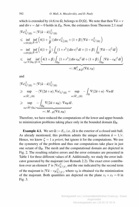
Example 4.1. We set Ω := E1, i.e., Ω is the exterior of a closed unit ball.As already mentioned, this problem admits the unique solution u = 1/r.Hence, we know ζ = 1 a priori, but ignore it for the computations. We usethe symmetry of the problem and thus our computations take place in justone octant of ΩR. The mesh and the computational domain are depicted inFig. 2. The resulting relative errors and the error estimates are presented inTable 1 for three different values of R. Additionally, we study the error indi-cator generated by the majorant (see Remark 2.2). The exact error contribu-tion over an element T is |∇e|2L2(T ) and the one indicated by the second term

of the majorant is |∇u− vR|2L2(T ), where vR is obtained via the minimizationof the majorant. Both quantities are depicted on the plane x1 + x3 = 0 inFig. 3.




(a) (b)Figure 2. Computational domains and meshes (one octant of ΩR, where R = 10) for Exam-ple 4.1 (a) and Example 4.2 (b).

(a) (b)Figure 3. Example 4.1, true error |∇e|2L2(T ) (a) and error indicator |∇u− vR|2L2(T ) (b).

The boundary value problem in Step 1 of Algorithm 4.1 was solvedby the finite element method. We applied first-order nodal tetrahedral ele-ments, where the mesh was constructed by Comsol 4.3 and the emergingsystem of linear equations was solved using a standard Matlab solver. Whenminimizing the majorant M2

+,R,β (∇u,vR) with respect to vR ∈ V(ΩR), weapplied second-order tetrahedral finite elements for each component of vR

with vR|SR =−ζ R−2eR and hence eR·vR|SR =−ζ/R2. Similarly, the minorantM−,R(∇u,uR) was maximized using second-order tetrahedral finite elements

for uR ∈H1(ΩR). A natural choice is to use H(div)-conforming Raviart–

Thomas elements [6] to compute vR. However, H1-elements are applicablefor smooth problems.




Table 1.Example 4.1, the exact error and the computed errorestimates.

R NtM2

+,R,β (∇u,vR)

|∇u|2L2(Ω)

|∇e|2L2(Ω)

|∇u|2L2(Ω)

M−,R(∇u,uR)|∇u|2L2(Ω)

5 1926 4.57% 3.75% 3.61%5 6223 1.39% 1.31% 1.29%5 17742 0.63% 0.62% 0.61%

10 2214 7.19% 5.68% 5.43%10 5264 2.82% 2.55% 2.51%10 11506 1.80% 1.68% 1.65%

20 3446 7.26% 5.73% 5.47%20 6676 2.95% 2.64% 2.60%20 13370 1.86% 1.74% 1.71%

Table 2.Error bounds for Example 4.2.

NtM2

+,R,β (∇u,vR)

|∇u|2L2(Ω)

M−,R(∇u,uR)|∇u|2L2(Ω)

2513 12.52% 4.65%5015 9.48% 2.91%

13772 7.08% 1.63%

Example 4.2. We set Ω := R3 \ [−1,1]3, i.e., Ω is the exterior of a closedcube. For this problem, the exact solution u is not known. The octant ofΩR for R = 10 used in the computations is depicted in Fig. 2. In Algo-rithm 4.1, we have selected uR,1 and uR,2 as finite element solutions ofDirichlet Laplace problems with proper boundary conditions. The respec-tive error bounds are presented in Table 2.

These examples show that functional a posteriori error estimates pro-vide two-sided bounds of the error. Of course, the accuracy depends on themethod used to generate the free variables v and u in the majorant and mi-norant, respectively. The applied methods should be selected balancing thedesired accuracy of the error estimate and the computational expenditures.

Appendix A. Easier but weaker estimatesWe want to point out that we can prove a variant of Theorem 3.1 by an-other, much simpler technique using just the triangle inequality instead of




the Helmholtz decomposition. The drawbacks are that we get for the upperbound a factor larger than 1, e.g., 5, which overestimates a bit more, and for

the lower bound we miss one term. To see this, let u∈H1−1(Ω)+u0. Then

|E|L2(Ω),A =∣∣∇u−A−1v

∣∣L2(Ω),A 6 |∇(u−u)|L2(Ω),A +

∣∣∇u−A−1v∣∣L2(Ω),A

and we can further estimate by Theorem 2.1 with u = u for any v ∈ D(Ω)

|E|L2(Ω),A 6 cN,α | f +divv|L21(Ω) +

∣∣∇u−A−1v∣∣L2(Ω),A︸︷︷︸

= M+(∇u,v)

+∣∣∇u−A−1v

∣∣L2(Ω),A

6 cN,α | f +divv|L21(Ω) +

∣∣A−1(v− v)∣∣L2(Ω),A︸︷︷︸

= M+(A−1v,v)

+2∣∣∇u−A−1v

∣∣L2(Ω),A︸︷︷︸

= M+(A−1v,∇u)

.

Therefore, we get the same upper bound, but with less good factors, i.e., forany θ > 0

|E|2L2(Ω),A 6 M+(v) :=(1+4θ

) infv∈D(Ω)

M2+(A−1v,v)

+(4+θ) infu∈H1−1(Ω)+u0

M2+(A−1v,∇u)

with M+(v) > M+(v). For example, for θ = 1 we have 1+4/θ = 4+θ = 5

and M+(v) = 5M+(v). For the lower bound and u ∈H1−1(Ω) we simply

have

|E|2L2(Ω),A =∣∣∇u−A−1v

∣∣2L2(Ω),A

> 2⟨∇u−A−1v,∇u

⟩L2(Ω),A−|∇u|2L2(Ω),A

= 2〈 f ,u〉L2(Ω)−⟨∇u+2A−1v,∇u

⟩L2(Ω),A = M−(A−1v,u)

and the additional term M−(A−1v,A−1v,∇u) does not appear. Thus,

|E|2L2(Ω),A > M−(v) := supu∈H1−1(Ω)

M−(A−1v,u)

with M−(v) 6 M−(v).

Acknowledgement

We heartily thank Sergey Repin for his continuous support and many inter-esting and enlightening discussions.




References

1. R. Courant and D. Hilbert, Methoden der Mathematischen Physik, Band 1. Springer,Heidelberg, 1924.

2. R. Leis, Initial Boundary Value Problems in Mathematical Physics. Teubner, Stuttgart,1986.

3. O. Mali, P. Neittaanmaki, and S. Repin, Accuracy verification methods, theory andalgorithms (in print).

4. P. Neittaanmaki and S. Repin, Reliable Methods for Computer Simulation, Error Con-trol, and A posterioroi Estimates. Esliver, New York, 2004.

5. D. Paule and S. Repin, Functional a posteriori error estimates for elliptic problems inexterior domains. J. Math. Sci. N. Y. (2009) 162, No. 3, 393–406.

6. P. A. Raviart and J. M. Thomas, Primal hybrid finite element methods for 2nd orderelliptic equations. Math. Comp. (1977) 31, 391–413.

7. S. Repin, A posteriori error estimates for variational problems with uniformly convexfunctionals. Math. Comp. (2000) 69, No. 230, 481–500.

8. S. Repin, A posteriori estimates for partial differential equations. Radon Series Comp.Appl. Math. Walter de Gruyter, Berlin, 2008.

9. S. L. Sobolev, Partial Differential Equations of Mathematical Physics. Oxford Univer-sity Press (Pergamon Press), New York, 1964.



Conforming and non-conforming functional a posteriori ...

Documents

Transcript of Conforming and non-conforming functional a posteriori ...