Classical Conditioning. Experiencing Classical Conditioning.

Conditioning Prices on Search Behaviour�
Mark Armstrong
University College London
Jidong Zhou
University College London
January 2010
Abstract
We consider a market in which �rms can partially observe each consumer�s
search behavior in the market. In our main model, a �rm knows whether a
consumer is visiting it for the �rst time or whether she is returning after a previous
visit. Firms have an incentive to o¤er a lower price on a �rst visit than a return
visit, so that new consumers are o¤ered a �buy-now�discount. The ability to o¤er
such discounts acts to raise all prices in the market. If �rms cannot commit to
their buy-later price, in many cases �rms make �exploding�o¤ers, and consumers
never return to a previously sampled �rm. Likewise, if �rms must charge the same
price to all consumers, regardless of search history, we show that they sometimes
have the incentive to make exploding o¤ers. We also consider other ways in which
�rms could use information about search behaviour to determine their prices.
Keywords: Consumer search, oligopoly, price discrimination, high-pressure sell-ing, exploding o¤ers, costly recall.
1 Introduction
In a variety of markets in which consumers sequentially search through �rms�options,
sellers know something about their potential customers�search behaviour. For example,
a seller may be able to distinguish visitors who come to the store for the �rst time from
those who have returned after a previous visit. Salesmen may try to elicit information
from a customer about how many other sellers she has already sampled and how many
more she plans to sample. In online markets, sellers may be able to monitor the entire
search process of a potential customer.
�We are grateful to Simon Anderson, Marco Haan, Preston McAfee, Meg Meyer, Andrew Rhodes
and Asher Wolinsky, and to the Economic and Social Research Council (UK) and the British Academy
for funding assistance.
1

There are two broad reasons why a �rm may wish to condition its price on a con-
sumer�s search behaviour. First, search history may reveal relevant information about
a consumer�s tastes. For example, a seller may wish to charge a higher price to those
consumers who have already investigated other sellers, because their decision to keep
searching indicates they are unsatis�ed with previously sampled products when search
is costly. (If consumers have heterogenous search costs, it may also reveal that such
consumers have relatively low search costs, which may by contrast induce a seller to set
a low price.) Second, �rms may have a strategic reason to condition its price on search
history, which is to deter a potential consumer from going on to search rival o¤ers. For
example, if a �rm can distinguish new visitors from consumers who have previously
visited, a �rm can o¤er new customers a relatively low price or force them to buy its
product now or not at all, which makes customers more reluctant to investigate rival
o¤ers. This paper investigates whether setting prices conditional on search behaviour,
if feasible, can emerge as an equilibrium outcome, and, if so, how this practice a¤ects
market performance.
Our underlying framework is a duopoly sequential search model with horizontally
di¤erentiated products in which consumers search both for price and product �tness.
Each �rm has three sources of demand: consumers who sample its product �rst and buy
immediately (�fresh consumers�), consumers who sample the �rm �rst, go on to sample
the rival�s product, but eventually come back (�returning consumers�), and consumers
who sample the rival �rst but go on to buy from the �rm in question (�incoming
consumers�). In the standard search model, �rms cannot distinguish between these
three groups and so o¤er the same price to all their visitors. In our models, �rms
are able to recognize and price discriminate between at least some of these di¤erent
consumer groups.
In our main model, presented in section 3, �rms can distinguish returning consumers
from other consumers (i.e., they can tell old faces from new faces), and can charge
them a di¤erent price. We show that in equilibrium the price for returning consumers
is higher than that o¤ered to others, or equivalently the consumers who visit a �rm
for the �rst time will be o¤ered a �buy-now discount�. Consumers are therefore more
reluctant to sample the rival �rm�s product. Due to this e¤ect, even the discounted
buy-now price is higher than the non-discriminatory price. As such, this form of price
discrimination lowers both consumer surplus and total welfare. When the search cost
is relatively high, price discrimination will lead to excessively high prices even from the
�rms�perspective, and the ability to o¤er buy-now discounts reduces industry pro�ts.
In section 3.3 we relax our assumption that �rms commit to their buy-later price when
consumers make their �rst visit. When �rms can commit to an upper bound on buy-
later prices (e.g., by displaying a credible �regular price�on the shop shelves) then the
full commitment outcome is still achieved. When �rms have no commitment power,
2

we argue that they are often forced to make �exploding o¤ers�, i.e., new visitors are
forced to buy immediately or not at all. In section 3.4, we present a related model
in which �rms cannot price discriminate but can arti�cially in�ate a consumer�s cost
of returning. (Thus, only the �strategic e¤ect�mentioned above is relevant.) In this
situation, we derive conditions under which �rms choose to make exploding o¤ers.
In section 4, we investigate other ways in which �rms can condition their prices
on search behaviour. We �rst suppose that �rms can distinguish all three groups of
consumers and so, in principle can set three di¤erent prices. We show that �rms in
equilibrium will set the same (high) price to returning and to incoming customers,
and o¤er a discount only to fresh customers. Thus, �rms discriminate equally against
those customers who have sampled the rival, regardless of whether they are incoming
or returning customers. We then consider the case in which each �rm can distinguish
consumers who sample it �rst (i.e., fresh and returning consumers) from those who
sample its rival �rst (i.e., incoming consumers). Since incoming consumers must be
unsatis�ed with the rival�s product, in equilibrium �rms charge them a high price.
There has apparently been little research exploring the question of how �rms might
make use of knowledge of consumer search behaviour or search history to re�ne their
pricing decisions. Nevertheless, as we discuss next, our paper relates to several strands
of the industrial organization literature. In the recent literature on ordered search,
consumers sequentially search through options according to some publicly known order,
which automatically reveals part of their search history to sellers. Armstrong, Vickers,
and Zhou (2009) consider a model where consumers search for both price and product
�tness (as in this paper) and where consumers consider one �prominent��rm �rst. In
equilibrium the prominent �rm sets a lower price than the others: �rms further back
in the search order know that any customer who reaches them does not particularly
value the previous o¤ers made, and so such �rms can exploit their market power by
setting a higher price. (This paper is discussed further in section 4 below.) Arbatskaya
(2007) analyzes a related model where consumers care only about price but di¤er in
their search cost. She obtains the reverse �nding, which is that �rms further back in
the search order set lower prices. Intuitively, this is because these �rms are only visited
by consumers with relatively low search costs and so face more competition.1
Related e¤ects can be obtained in models of simultaneous, as opposed to sequential,
search. For instance, in a di¤erentiated product setting, Gal-Or, Gal-Or, and Dukes
(2007) suppose that the buyer can announce from how many sellers she is soliciting
quotes, and sellers can condition their price on that information. As is intuitive, in
many cases (see their Corollary 1 ) �rms o¤er a lower price when they know they
1More distantly related is the idea of a �stigma e¤ect�of long-term unemployment. For instance,
Vishwanath (1989) supposes that potential employers can observe how many times a worker has failed
to generate a job o¤er, and can condition wage o¤ers on this variable.
3

must compete against more rivals. Deck and Wilson (2006) conduct an experimental
study of a related market. Firms (played by experimental subjects) sell a homogenous
product, and consumers (played by price-minimizing robots) are exogenously divided
into several groups according to the number of �rms they sample. Each �rm knows how
many other �rms a consumer samples and can condition the price on that information.
In their experiment, more informed consumers are treated better when sellers can price
discriminate relative to when sellers do not observe a consumer�s search behaviour.
In our main model �rms o¤er a �buy-now�discount, and this acts to increase the
cost of returning to a previous �rm. As such, our analysis is related to models of search
with costly recall. Janssen and Parakhonyak (2008) study the optimal stopping rule
when consumers care only about price and must incur a cost to return to a previous
�rm. This stopping rule is signi�cantly more complicated than when return is costless.
When there are more than two �rms, a consumer�s stopping rule is non-stationary, her
reservation surplus level is not independent of her previous o¤ers, and a consumer may
end up buying a product which is more expensive than others she has sampled. (This
is the pragmatic reason why we focus on a duopoly model, where these complexities
are absent.) However, in their model, the supply side is passive and sellers�prices are
randomly drawn from an exogenous distribution. Our paper is also related to models of
search with endogenous recall. Daughety and Reinganum (1992) make the point that
the extent of consumer recall may be endogenously determined by �rms�equilibrium
strategies. In their model, the instrument that a �rm can use to in�uence consumer
recall is the length of time that it will hold the good for consumers at the quoted price.
(In our main model, that instrument is the buy-now discount.) In contrast to our
assumption that a consumer can discover a seller�s return cost only after investigating
that seller, Daughety and Reinganum suppose that sellers can announce their recall
policies to the population of consumers before search begins.
Our paper relates also to situations with high-pressure selling. Broadly speaking,
�high-pressure selling�can be classi�ed into at least two types. One type aims to �per-
suade�(maybe boundedly rational or socially nervous) consumers to buy unnecessary
or over-priced products such as some extended warranties, some payment protection
insurance, and so on.2 Another type of high-pressure selling aims to reduce the con-
sumer�s incentive to search further. For example, the seller can commit (or at least
claim) that the current price o¤er� or even the availability of the product� will expire
if consumers do not buy immediately. Sellers of �nancial products may sometimes at-
tempt this sales technique, especially if they are in the home, and the practice is also
used in some specialized labour markets.3
2See, for instance, Chu, Gerstner, and Hess (1995) for a model of this type of persuasive high-
pressure selling.3One of the authors encountered an in-home salesman of �nancial products, and when he said he
4

Firms often bene�t from the reduction of consumer search intensity, since this usu-
ally softens price competition. In our model, the buy-now discount or the exploding
o¤er serves this purpose. Alternatively, Ellison and Wolitzky (2008) present a model in
which consumers have convex search costs (i.e., a consumer�s incremental search cost
increases with her cumulative search e¤ort). Then if a �rm increases its in-store search
cost (say, by making its price harder to comprehend), it will make further search more
costly, and thus less likely. Though very di¤erent, the two models lead to a similar
result that, even if the exogenous search cost tends to zero, the market may not be
frictionless in equilibrium.
De los Santos (2008) presents a rare empirical study of individual consumer search
behaviour prior to making a purchase, using data from online book purchases. In this
particular market there is no evidence of price discrimination of the kind we study in this
paper (as far as we know), but the patterns of search behaviour are nevertheless relevant
for our work. In his data, De los Santos (2008, section 4) �nds that three-quarters
of consumers search only one retailer before making their purchase, i.e., using our
terminology, fresh demand makes up 75% of total demand. Of the remaining consumers
who search at least twice, approximately two-thirds buy from the �nal �rm searched
(�incoming demand�) and one-third go back to a �rm searched earlier (�returning
demand�). De los Santos also �nds that the initial search is non-random (unlike our
main model below), and one �rm (Amazon.com) was sampled �rst by about two-thirds
of all consumers making a purchase. (We discuss the impact of having one �rm more
prominent in section 5 below.)
Our analysis of buy-now discounts is also somewhat related to the emerging lit-
erature on auctions with a �buy now� price (see Reynolds and Wooders (2009), for
instance). Online auctions such as those run by eBay sometimes o¤er bidders the op-
tion to buy the item immediately at a speci�ed price rather than enter an auction
against other bidders. In these situations, a seller has one item to sell to a number of
potential bidders, and so a bidder needs to pay a high buy-now price in order to induce
the seller from going on to �search�for other bidders by running an auction, whereas
our model involves sellers o¤ering a low buy-now price so as to induce a buyer from
going on to search for other sellers. Common rationales for buy-now prices in auctions
are impatience or risk-aversion on the part of bidders, neither of which is needed in our
framework with costly search.
Although there is not a great deal of work on conditioning prices on search history,
wished to think about the o¤er and get back to the salesman, the salesman claimed it was his last
day in his current job. Roth and Xing (1994, page 1001) document some examples of high-pressure
job o¤ers. For instance, in the market for judicial clerkships, some judges use exploding o¤ers which
would be withdrawn if they are not accepted in some very short time, or even during the telephone
conversation itself.
5

there is a substantial literature about how �rms can use the information of consumer
purchase history to re�ne their pricing decisions. See, for instance, Hart and Tirole
(1988), Chen (1997), Fudenberg and Tirole (2000), and Acquisti and Varian (2005).
These models often predict that a �rm will price low to a customer who previously
purchased from a rival (or consumed the outside option in the case of monopoly), since
such a customer has revealed she has only a weak preference for the �rm�s product. In
the current paper, though, we will see that a �rm will price high to a customer who
previously searched a rival, since that customer has revealed she has relatively weak
preferences for the rival�s product.
2 A Model and Preliminary Results
Our underlying model of consumer choice is based on Wolinsky (1986), simpli�ed to
duopoly.4 (See Anderson and Renault (1999) for a further development of Wolinksy�s
model.) There are two �rms i = A;B in the market, each supplying a horizontally
di¤erentiated product at zero production cost. A consumer�s valuation of product i,
ui, is a random draw from some common distribution with support [0; umax] and with
cumulative distribution function F (�) and density f(�). We suppose that the realizationof match utility is independent across consumers and products. In particular, there
are no systematic quality di¤erences across the products. Each consumer has a unit
demand for only one product, and for expositional simplicity the number of consumers
is normalized to two.
Consumers initially have imperfect information about prices and match utilities.
But they can gather this information through a sequential search process: by incurring
a search cost s � 0, a consumer can visit a �rm and �nd out its price and match value.5
After sampling the �rst �rm, a consumer can choose to buy at this �rm immediately or
continue on to investigate the second �rm. If she continues to search, she can buy from
the second �rm or return to buy from the �rst �rm, or neither. If she returns to buy
from the �rst �rm, she does not incur a further search cost.6 We focus on symmetric
4Note that if there were in�nitely many �rms, there is no role for conditioning prices on search
history. Even if consumers can costlessly return to a previously sampled product, when consumers
have unlimited options it is a standard result in search theory that consumers optimally do not return
to previous options, but always prefer to search for a new option. Note also that this duopoly model
applies when there are more than two sellers if, for some reason, consumers never consider more than
two options.5If the search cost is zero, we require that consumers nevertheless consider products sequentially.6Our analysis could straightforwardly extend to situations where consumers have an intrinsic cost
of returning to a previously sampled �rm, but few new insights emerge with that extension. The
main exception is in section 3.3, where we consider the situation where �rms cannot commit to their
buy-later price and show that the presence of even a small returning cost will shut down the market
for returning customers altogether.
6

situations in which half the consumers sample �rm A �rst, while the other half �rst
sample B.7 Each �rm has three sources of demand: consumers who sample its product
�rst and buy immediately (�fresh consumers�), consumers who sample its product �rst,
go on to investigate the rival �rm, but eventually come back (�returning consumers�),
and consumers who sample its rival �rst but go on to buy from the �rm in question
(�incoming consumers�).
Firms maximize their pro�ts, and set prices simultaneously based on their expec-
tation of consumer behavior. However, their pricing decisions depend on how much
information they have about consumers�search history. If all consumers are indistin-
guishable, as in Wolinsky (1986), each �rm must set a uniform price. But if some groups
of consumers are distinguishable, �rms may be able to price discriminate. There are
a number of di¤erent kinds of price discrimination which could be considered. In our
main model, analyzed in section 3, we suppose that �rms can distinguish returning con-
sumers from other consumers, but cannot distinguish incoming from fresh consumers.
For instance, this might apply when a consumer needs to interact with a seller to discuss
speci�c requirements which reveal the consumer�s identity, and it is therefore clear if a
consumer has previously consulted the seller. (Examples might include job o¤ers, med-
ical insurance, or home improvements.) Likewise, in online markets sellers might place
�cookies� on a consumer�s computer which reveal whether the consumer has visited
previously. In such cases, it is often the case that a seller does not know whether the
consumer has also interacted with rival sellers. In section 4, we consider the alternative
situation in which a �rm does observe whether a consumer has visited a rival.
When a �rm sets a higher price to returning customers than to customers on their
�rst visit, a customer faces a returning cost if she chooses to leave and then return
to the �rm, since the price she has to pay will then rise. Similarly, in our model of
high-pressure selling in section 3.4, �rms impose a non-monetary returning cost. As
a necessary ingredient for each of these models, we next derive the optimal stopping
rule for consumers in a search model with an arbitrary (monetary or non-monetary)
returning cost, which may be �rm speci�c and is denoted � i.
A consumer�s optimal stopping rule balances the surplus of the �rst sampled product
and the expected surplus from searching on. Denote by
V (p) �Z umax
p
(u� p) dF (u)� s (1)
the expected surplus of sampling the second product if a consumer expects that the
second �rm will charge price p and she surely does not return to buy the �rst product.
De�ne
a� � z� + � ; (2)
7We discuss the impact of one �rm being more prominent in section 5 below.
7

where z� solves
V (z� ) � � : (3)
Note that both z� and a� decrease with � . Indeed,
da�d�
=�F (z� )1� F (z� )
: (4)
As we show next, a� determines the consumer�s reservation utility level when she an-
ticipates a returning cost � if she leaves and then returns to a �rm. That is, if the
two �rms charge the same tari¤s, a consumer will investigate the second �rm when the
match utility of the �rst product is below a� . In more detail:
Lemma 1 Consider a consumer who encounters �rm i �rst and is o¤ered the price
pi and match utility ui. Suppose the consumer expects that �rm j will charge p with
V (p) > 0 and expects that she will incur a returning cost � i if she returns to �rm i after
sampling �rm j (in addition to �rm i�s price pi).
(i) If � i < V (p), she will search on to �rm j if and only if
ui � pi < a� i � p ; (5)
and she will return to �rm i after sampling �rm j if ui � pi � � i > maxf0; uj � pjg,where pj is �rm j�s actual price.
(ii) If � i � V (p), she will search on to �rm j if and only if
ui � pi < V (p) ;
and she will never return to �rm i after sampling �rm j (regardless of �rm j�s actual
price pj).
(All omitted proofs can be found in the Appendix.)
Note that when � i = V (p), the cut-o¤ surplus levels in cases (i) and (ii) coincide.
Note also that in case (i) some consumers will indeed return to �rm i after investigating
�rm j. Those consumers with match utility just below the threshold in (5) will go on
to investigate j, and if j�s match utility is low (below pj say), then the consumer still
obtains positive utility if she returns to i.8
When there is no returning cost (� i = 0), Lemma 1 implies that the consumer will
sample the second �rm whenever ui�pi < a0�p.9 This is the stopping rule in the search8Formally, when ui � a� i+pi�p so that (5) is nearly satis�ed, then ui�pi�� i � a� i�� i�p = z� i�p,
which is positive since V (�) is a decreasing function and by assumption V (z� i) = � i < V (p).9Notice that the stopping rule also applies for a negative returning cost � i � �s. (If � i < �s,
consumers will always sample the second product.) We show later that this does not occur in equilib-
rium. In addition, if � i < 0 (which might occur if a �rm�s buy-later price p̂i is lower than its buy-now
price pi) then a consumer has an incentive to leave �rm i and return, even if she has no intention of
investigating the rival. If this kind of consumer arbitrage behavior� of stepping out the door and then
back in again� cannot be prevented, then setting p̂i < pi is equivalent to setting a uniform price p̂i,
and so without loss of generality we can assume �rms are constrained to set � i � 0.
8

model with costless recall as described in Wolinsky (1986). Since a� decreases with the
returning cost � , it follows that if the returning cost increases, a consumer becomes less
willing to investigate the rival �rm. (The utility from sampling the rival falls with �
since there are fewer pro�table opportunities to return to the initial �rm.) The case
where � i < V (p) is illustrated in Figure 1, where the shaded area is the region where the
consumer buys neither product. (Recall that p is the price which consumers anticipate
�rm j will charge, while pj is the price that �rm j actually o¤ers.) When � i exceeds
V (p), the returning cost is so great that the consumer never returns to �rm i once she
leaves it and returning demand vanishes. Hence, the continuation payo¤ for sampling
the second �rm is V (p), and she will sample both products whenever ui � pi < V (p).
-
6
�����������
0 pi + � i a� i + pi � pui
uj
pj buy product iafter sampling j
(i�s returningdemand)
buy product iimmediately
(i�s fresh demand)
buy product j
(j�s incoming demand)
ppppppppppppppppppppppppppppppppppppppppppppppppppppppppppppppppppppppppppppppppppppppppppppppppppppppppppppppppppppppppppppppppppppppppppppppp
Figure 1: Pattern of demand for consumers who sample �rm i �rst (� i < V (p))
In the remainder of the paper, an important consideration is whether a higher cost
for returning to a �rm acts to boost or reduce that �rm�s total demand. First, it is
clear that a �rm�s returning cost � i cannot a¤ect its incoming demand, since incoming
consumers buy immediately or not at all. Second, Figure 1 shows that increasing � iboosts a �rm�s fresh demand. Third, the �gure also shows that the �rm�s returning
demand contracts with a higher � i. Thus, the impact on the �rm�s total demand is
unclear a priori. The next result discusses the net impact in some special cases:
Lemma 2 Suppose that �rm j�s actual incoming price pj is equal to the anticipated
price p. Then an increase in �rm i�s returning cost � i will:
(i) increase the �rm�s total demand if the density f is increasing with u;
9

(ii) decrease the �rm�s total demand if the density f is decreasing with u;
(iii) leave the �rm�s total demand unchanged if u is uniformly distributed.
The intuition for this result is as follows. A fresh consumer who buys at �rm i
immediately has a higher valuation of the product than a returning consumer. When f
is increasing, there are more consumers with higher valuations in the population, and
so the e¤ect of a higher recall cost on increasing fresh demand is more signi�cant than
its impact on returning consumers. When f is decreasing, the opposite is true. When
utilities are uniformly distributed, the net impact of the returning cost on total demand
is zero, and an increase in � i causes demand to be substituted from returning to fresh
demand in a one-for-one manner.
As discussed earlier, a �rm has two broad reasons to condition its o¤er on a con-
sumer�s search behaviour: an informational motive based on what it learns about the
consumer�s preferences, and a strategic motive to in�uence the consumer�s decision to
engage in further search. The strategic motive is essentially captured by the impact
of the return cost on a �rm�s total demand. Thus, if the density is increasing, a �rm
has an incentive to make it hard for consumers to return to it, as the resulting gain
in fresh demand outweighs the loss of returning customers. As we discuss further in
section 3.4, this implies that when the density is increasing, �rms have an incentive to
force potential consumers to buy �now or never�.
3 �Buy-Now�Discounts
Consider the situation in which �rms are able to recognize returning consumers and
charge them a di¤erent price. Each �rm then potentially sets two prices: pi is �rm i�s
price to those consumers who visit it for the �rst time (comprising both the fresh and
incoming consumers), while p̂i is its price o¤ered to a consumer when she returns to
the �rm. An interpretation is that each �rm sets a �regular�(or �buy-later�) price p̂iand o¤ers the �rst-time visitors a �buy-now�discount � i � p̂i � pi. We assume that a�rm can commit to p̂i when it o¤ers new visitors the buy-now price pi. (We discuss the
impact of more limited commitment later in section 3.3.)
For simplicity, from now on we focus mostly on the case where match utility ui is
uniformly distributed on [0; 1], so that F (u) � u and expression (2) becomes
a� = 1 + � �p2(s+ �) :
As we saw in Lemma 2, this assumption essentially shuts down a �rm�s �strategic�
motive to make return more costly, since a �rm�s total demand is una¤ected by its
return cost with a uniform distribution. This greatly simpli�es the algebra and enables
us to check second-order conditions for the candidate equilibrium. However, our main
10

result that �rms will choose to o¤er a buy-now discount continues to hold for more
general distributions for the match utility, provided that the density function for u
does not decrease �too fast�. (See Table 1 below for illustrations of the equilibrium
when the distribution of match utility is non-uniform.)
To ensure an active market we assume a relatively small search cost 0 � s � 18. (If
s > 18then there is no equilibrium in which consumers sample even one �rm�s o¤er.)
We also focus on symmetric equilibria where both �rms o¤er the same price pair (p; p̂).
3.1 Equilibrium prices
For convenience, we analyze the model in terms of the buy-now price p and the total
returning cost � = p̂� p (rather than in terms of p and p̂). Suppose �rm j adopts the
equilibrium strategy (p; �) and consumers expect that both �rms will o¤er these prices.
If �rm i unilaterally deviates to (pi; � i), with � i � V (p), its pro�t is10
piQT + � iQR ; (6)
where QT is �rm i�s total demand and QR is the portion of demand from its returning
customers. (The �rm obtains revenue pi from all its customers, plus the incremental
revenue p̂i � pi = � i from its returning customers.) These demand functions can be
derived by calculating the areas of the various regions in Figure 1 to yield11
QT = 1� (pi + a� i � p)| {z }fresh demand
+1
2(a� i � � i)2 �
1
2p2| {z }
returning demand QR
+ a� (1� pi)�1
2(a� � p� �)2| {z }
incoming demand
: (7)
Note that the �rm�s returning demand does not depend on its buy-now price pi over
the relevant range. (By examining Figure 1, we see that varying pi simply shifts the
region of returning demand uniformly to the left or right.) Note also that the �rm�s
total demand QT does not depend on its buy-now discount � i. (This follows from part
(iii) of Lemma 2.) Thus, a �rm�s pro�t in (6) is additively separable in its buy-now
price pi and its buy-now discount � i.
In particular, �rm i will choose its returning cost � i to maximize � iQR(� i), the
extra revenue from its returning consumers. We deduce that given the equilibrium
buy-now price p, the buy-now discount � maximizes the incremental industry pro�t
from returning customers, which is
�((a� � �)2 � p2) = �(z2� � p2) : (8)
10When � i � V (p), the returning demand disappears and fresh demand becomes 1� [pi+V (p)]; andso the pro�t will be independent of � i. Hence, our restriction to � i � V (p) is without loss of generality.11To calculate �rm i�s incoming demand use Figure 1 to calculate �rm j�s incoming demand, but
permute the two �rms, i.e., replace pj with pi and replace pi with p. (A consumer who visits �rm j
�rst expects that �rm i will o¤er the equilibrium price p, although �rm i in fact has price pi.)
11

It is clear (e.g., by using a revealed preference argument) that the value of � which
maximizes (8) is a decreasing function of p.12 In equilibrium, as we will show, we
have p < a0 = z0 provided that s < 18. Since z� is a decreasing function of � , it
follows that the pro�t generated from returning consumers in (8) is negative whenever
� < 0, and strictly positive for � in a neighborhood above 0. We deduce that �rms
in equilibrium will choose a strictly positive buy-now discount if s < 18. Note that a
�rm has an incentive to o¤er a positive buy-now discount even if its rival does not.
Moreover, returning demand falls to zero if � � V (p), i.e., if z� � p, and from (8) we
can deduce that in equilibrium p < z� whenever s < 18. From Figure 1, it follows that
there is indeed a region of returning demand in equilibrium. That is to say, although
�rms could force consumers to buy �now or never� by choosing a very large � , it is
more pro�table for them to induce at least some consumers to return after sampling
the rival�s o¤er and to extract some additional revenue � from them.
One can show that (8) is concave in � in the (relevant) region 0 � � � 18(and is
decreasing in � for larger �).13 From (8) and noting that dz�=d� = �1=(1 � z� ), the�rst-order condition for equilibrium � given p is
z2� � p2 �2�z�1� z�
= 0 : (9)
Turning to the equilibrium choice of buy-now price p, note that �rm i�s total demand
in (7) is linear in pi, and so its pro�t is concave in pi. Therefore, the �rst-order condition
for pi to be optimal is also su¢ cient. Each �rm�s equilibrium total demand is QT =
1� p(p+ �). That is, a consumer will leave the market without buying anything if andonly if she neither buys at the second �rm nor wants to go back to the �rst one. Using
this fact, one can see that the �rst-order condition for the equilibrium buy-now price
p, given � , is1
p� p = 1 + z� + 2� : (10)
The right-hand side of (10) is at least 32.14 Since the left-hand side of (10) is decreasing in
p, it follows that the solution to this �rst-order condition satis�es p � 12. (In particular,
since a0 = z0 � 12, it follows that p < a0 = z0 as claimed previously.) Moreover,
for 0 � � � 18� s, which will be the relevant range of � , the right-hand side of (10)
12More precisely, the �rm�s optimal choice for � i decreases with its rival�s buy-now price.13Expression (8) is decreasing in � if and only if z2� � p2 + 2�z�z0� < 0, which is certainly true if
z� + 2�z0� < 0. But since z0� = �1=(1 � z� ), this is true if 2� > z� (1 � z� ), which in turn is always
true if � > 18 . Thus, pro�t decreases in � for � >
18 . Next, suppose that � �
18 . Di¤erentiating the
�rst-order condition once more shows that (8) is concave in � if and only if � < 2z� (1 � z� )2, i.e., if�=(s+ �) < 4(1�
p2(s+ �)). But when s; � < 1
8 the right-hand side of this is greater than 1, and so
the claim follows.14Note that z� + 2� is a convex function which is minimized by setting � = 1
8 � s, which makes theright-hand side of (10) equal to 7
4 � 2s. Since s �18 , the claim follows.
12

is decreasing in � , and so the buy-now price p in (10) is an increasing function of � .
Intuitively, a buy-now discount increases search frictions in the market, which in turn
allows �rms to charge a higher price.
As an aside, note that expression (10) reveals the equilibrium price in the alterna-
tive situation where �rms choose a uniform price p and consumers have an exogenous
returning cost � for returning to a previously-sampled �rm. (In this situation, �rm i�s
pro�t is modi�ed from (6) to be piQT , where we set � i = � in (7). The �rst-order
condition for the equilibrium price is therefore still (10).) As far as we know, this is
only example where equilibrium price is derived in an oligopoly model with a returning
cost.15
The equilibrium strategy (p; �) is then found by solving the pair of nonlinear equa-
tions (9)�(10), which can typically be done only numerically. For instance, when s = 0,
so that there are no intrinsic search frictions in the market, solving these equations
shows that p � 0:45 and � � 0:06 and hence a buy-later price of p̂ � 0:51 (which is
actually slightly above the monopoly price of 0.5). In this example, although the mar-
ket has no intrinsic search frictions, �rms in equilibrium impose �tari¤ intermediated�
search frictions on consumers via the buy-now discount, which here is about 12% of
the buy-later price. By contrast, in a market with s = 18, which is the highest intrinsic
search cost which induces consumers to participate, one can check that the (exact) so-
lution to this pair of equations is p = 12and � = 0, so that there is no buy-now discount.
(When s = 18, search costs are so high that consumers will accept the �rst o¤er which
yields them a non-negative surplus. In particular, there are no returning consumers
even with costless recall.)
More generally, the equilibrium buy-now discount � decreases with the search cost
s. That is, the higher is the intrinsic search cost, the less incentive �rms have to deter
consumers from searching on. This can be seen from Figure 2A below, which depicts
how the buy-later price p̂ = p + � (the upper solid curve) and the buy-now price p
(the middle solid curve) vary with s. As is expected, the buy-now price increases with
the search cost. Less expected is the observation that the buy-later price depends
non-monotonically on s (and is always above the monopoly price).
Further details of the equilibrium are provided in this formal result.16
Proposition 1 Given s 2 [0; 18], the system of (9) and (10) has a solution (p; �) 2
[0; 12]� [0; 1
8� s], and the solution satis�es p � z� .
15As mentioned in the Introduction, Janssen and Parakhonyak (2008) examine consumer behaviour
in a model where consumers incur a recall cost. Although their model is in other respects more general
than ours, they do not model �rms�price choices.16As discussed, � decreases with p in (8) and p increases with � in the range 0 � � � 1
8 � s in (10),and so there is a unique equilibrium with (p; �) 2 [0; 12 ]� [0;
18 �s]. Numerical simulations suggest that
in the wider region of (p; �) 2 [0; 1]2 there are no other equilibria.
13

This analysis assumes that �rms cannot distinguish fresh from incoming customers
and so must charge both groups the same price. In section 4 we suppose instead that
�rms can distinguish all three customer groups, in which case it turns out that �rms will
o¤er incoming consumers the same price as the returning consumers, a price which is
higher than that o¤ered to fresh customers. Thus, if feasible, �rms have an incentive to
discriminate against customers who have investigated the rival �rm (i.e., the returning
and incoming customers), rather than discriminate between returning customers and
those customers who come to the �rm for the �rst time.
3.2 Comparison with uniform pricing
In the more familiar search model where �rms can only charge a uniform price p0,
consumers face no returning cost and so expression (10) implies that the �rst-order
condition for the price is1
p0� p0 = 1 + a0 : (11)
(Unlike the discriminatory prices, this uniform price can be explicitly computed.) Recall
that the price which solves (10) increases with the returning cost � for � 2 [0; 18� s].
We can therefore deduce the following result immediately:
Proposition 2 Price discrimination over returning consumers leads to higher prices,i.e., p0 � p � p̂.
That is, even the discounted buy-now price in the discriminatory case is higher than
the uniform price, and the ability to o¤er discounts for immediate purchase drives up
both prices.17 The intuition for this comes in two steps. First, a �rm�s total demand
is inelastic with respect to changes in the buy-now discount (perfectly so when match
utility is uniformly distributed). Since a �rm makes additional pro�t of � i from its
returning customers, it surely wishes to set a positive buy-now discount. Second, the
buy-now discount adds to the intrinsic search frictions in the market, and this allows
�rms to charge a higher price. (Relative to the uniform-price case, consumers become
less willing to search on, and so the �rms�demand is less price elastic.) Figure 2A
depicts the three prices, where from the bottom up the three curves represent p0, p
and p̂, respectively. In particular, when s = 18the search cost is so high such that no
consumers want to search beyond the �rst sampled �rm, there is no returning demand
in either regime, and so all three prices coincide.
In the discriminatory case, each �rm�s equilibrium demand is 1� pp̂. This is clearlylower than the counterpart 1�p20 in the uniform-pricing case since p; p̂ � p0. Hence, this17It is not unusual that the ability to price discriminate in oligopoly leads to falls in all prices, but
cases where all prices rise are less familiar.
14

form of price discrimination excludes more consumers from the market. In addition,
one can show that fresh demand rises, and returning demand falls, when this form of
price discrimination is used. This is illustrated in the case s = 0 in Table 2 below.
However, whether price discrimination leads to higher pro�t depends on the mag-
nitude of the search cost. In the non-discriminatory case, each �rm�s pro�t is �0 =
p0(1� p20). In the discriminatory case, from (6) each �rm�s pro�t is
� = p(1� pp̂) + 12�(z2� � p2) :
Figure 2B shows how �0 (the dashed curve) and � (the solid curve) vary with the
search cost s. We see that price discrimination leads to higher pro�t (i.e., � > �0)
only if the search cost is relatively small. When the search cost is relatively high, price
discrimination leads to prices which exclude too many consumers. In these cases, �rms
are engaged in a prisoner�s dilemma: when feasible an individual �rm wishes to o¤er a
buy-now discount, but when both do so industry pro�ts fall.18
0.00 0.02 0.04 0.06 0.08 0.10 0.12
0.42
0.44
0.46
0.48
0.50
0.52
s
Figure 2A: Prices and search cost
0.00 0.02 0.04 0.06 0.08 0.10 0.120.34
0.35
0.36
0.37
0.38
s
Figure 2B: Pro�ts and search cost
Finally, we observe that aggregate consumer surplus and total welfare (measured
by the sum of consumer surplus and pro�t) fall when �rms discriminate in this man-
ner. Consumer surplus falls since both prices rise compared to the non-discriminatory
regime. (Even if p̂ = p, i.e., if �rms charged returning consumers the buy-now price,
consumers would obtain lower surplus in the price-discrimination case since p � p0.
The buy-later premium � � 0 only adds to their loss.) As far as total welfare is con-cerned, relative to uniform pricing, price discrimination not only induces suboptimal
consumer search (i.e., consumers on average cease their search too early due to the
18This bears some similarities to situations with competitive bundling. There, a �rm often has a
unilateral incentive to o¤er consumers a discount for buying two products rather than one, but when
all �rms do this industry pro�ts fall. However, in contrast to the current case where the discount
relaxes competition and drives prices up, with bundling the discount intensi�es competition and drives
prices down. For instance, see Armstrong and Vickers (2010) for more details.
15

buy-now discount), but also excludes more consumers from the market, both of which
harm e¢ ciency.19
Our analysis of buy-now discounts so far has assumed that the match utility is uni-
formly distributed. It is possible to derive equilibrium prices in non-uniform examples
by calculating the measure, rather than simply the area, of the regions in Figure 1. As
a robustness check on our results, we report numerical calculations for the equilibrium
tari¤ in examples where the density function f is linear rather than constant. Speci�-
cally, suppose that the density takes the form f(u) = 2�u + 1 � �, where � 2 [�1; 1],so that the density function is a straight line with slope 2� passing through the point
(12; 1). Table 1 reports the equilibrium prices for various values of �, assuming that the
search cost s is zero.
� = �1 � = �0:5 � = 0 � = 0:5 � = 1
p0 0.312 0.382 0.414 0.405 0.360
p 0.313 0.392 0.450 0.474 0.470
� 0.017 0.032 0.060 0.091 0.124
�=(p+ �) 0.05 0.075 0.12 0.16 0.21
Table 1: Equilibrium prices when utilities are not uniformly distributed (s = 0)
Here, the �rst row reports the equilibrium non-discriminatory price, the second and
third rows report the buy-now price and discount, while the �nal row reports the buy-
now discount as a fraction of the buy-later price. The central column with � = 0 is
the uniform case previously discussed. As expected, when the density is increasing, the
incentive to set a buy-now discount is reinforced by an additional strategic e¤ect: as
shown in Lemma 2, with an increasing density a �rm�s total demand is boosted if it
makes it costly to return. Thus, we see that the size of the buy-now discount increases
with �, both in absolute terms and as a proportion of the buy-later price. Nevertheless,
over all linear density functions, the equilibrium buy-now discount remains positive.
Notice also that all prices are higher with price discrimination than without discrimi-
nation, even when the density is decreasing. In particular, consumers in aggregate are
worse o¤ with this form of price discrimination.
3.3 Buy-now discounts without commitment
We discuss next whether buy-now discounts can still emerge as an equilibrium outcome
if we relax the assumption that a �rm can commit to its buy-later price when consumers
�rst visit. We consider two cases: one with partial commitment in which �rms can
commit to a returning purchase price cap (but cannot commit to a speci�c price), and
19The proof of Proposition 3 in Armstrong, Vickers, and Zhou (2009) can be adapted to prove this
welfare result formally.
16
the other with no commitment at all. The �rst case may be reasonable in situations
where �rms can post a �regular� price. For example, the price printed on the price
label in a store usually has this kind of commitment power. The second case may be
more relevant in bargaining situations where it is infeasible to sign a contract for the
returning purchase price. In both cases, we argue that a buy-now discount can still
arise in equilibrium.
Partial Commitment: Here, there is an equilibrium with the same outcome as in thefull commitment case. Speci�cally, in this equilibrium, �rms charge a buy-now price p,
commit to a buy-later price cap p̂, and actually charge returning consumers p̂, where
both p and p̂ take the same values as the commitment case analyzed in section 3.1.
To sustain this equilibrium, we assume that all consumers believe that for any (maybe
o¤-equilibrium) committed price cap p̂i the �rm�s actual buy-later price will be p̂i.
To prove this claim, it su¢ ces to observe that when consumers hold the above belief,
they will return to the �rst sampled �rm, say �rm i, only if ui � p̂i, where p̂i is �rm
i�s buy-later price cap. This implies that �rm i can have no incentive to charge them
a price below p̂i. (It may have an incentive to raise the price above p̂i, but that is
not permitted given that the �rm commits to this cap.) This in turn ful�lls consumer
beliefs. Thus, the price cap can be used as a full commitment device.20
No Commitment: We turn next to the case where �rms can make no credible com-mitments about their buy-later prices when consumers �rst visit. Here, and unlike the
rest of this paper, it makes an important di¤erence whether or not consumers face an
intrinsic returning cost when they come back to a �rm. If consumers face no such cost
(as we assumed in the rest of the paper) it is possible to construct equilibria of the con-
stant markup form which are qualitively similar to the commitment prices: consumers
anticipate that a �rm will set a return price p̂i = pi + � if that �rm o¤ers the buy-now
price pi, and given these expectations �rms have no incentive to set a di¤erent buy-later
price. (There is a continuum of such � which can make up an equilibrium of this form,
and which induce some consumers to return to their initial �rm.) There is also an
�exploding o¤er�equilibrium: consumers anticipate that �rms o¤er very high prices if
they return and so never return, and given this behaviour �rms have no incentive to
reduce their return prices.
However, if there is even a small intrinsic returning cost, say r > 0, it turns out that
the only equilibrium involves exploding o¤ers where the returning demand segment is
shut down altogether. To see this, suppose in some equilibrium that each consumer
forecasts that a �rm�s buy-later price is p̂(pi) when its buy-now price is pi, where p̂(�)can take any form. Suppose that the buy-now price in this equilibrium is p�, say, and
20There may exist other equilibria involving di¤erent consumer beliefs.
17

suppose� contrary to the claim� there is some returning demand in this equilibrium.
(Formally, from Figure 1 this implies that r+p̂(p�)�p� < V (p�), where r+p̂(p�)�p� is aconsumer�s total returning cost.) But if a consumer returns to �rm i after �rst sampling
�rm i and then �rm j, it follows that her match utility satis�es ui � p̂(p�) + r, since
the consumer must also pay the returning cost r > 0. Since all its returning customers
have match utility at least p̂(p�) + r, the �rm�s optimal price for these customers must
be at least p̂(p�) + r, which contradicts the assumption that p̂(p�) was the correctly
anticipated buy-later price.
Thus, when there an intrinsic returning cost, no matter how small, consumers an-
ticipate that the buy-later prices will be so high that it is never worthwhile to return
to the �rst �rm after leaving it. In e¤ect, �rms are forced to make exploding o¤ers,
and consumers have just one chance to buy from any �rm. This result is analogous to
Diamond�s (1971) paradox, showing how a small search cost can cause a market to shut
down. Diamond�s result relies on consumers knowing their match utility in advance,
and one major advantage of Wolinsky�s formulation with ex ante unknown match util-
ities is that this paradox can be avoided. But even in our Wolinsky-type framework,
the returning consumers know their match utility, and so the returning market fails for
the same reason as the primary market failed in Diamond�s framework.
3.4 Non-monetary returning costs and exploding o¤ers
The previous section suggested that exploding o¤ers would often arise when �rms can-
not commit to their buy-later prices. In this section we discuss an alternative rationale
for exploding o¤ers. In the buy-now discount model, the discount � induces a return-
ing cost, but it also directly a¤ects �rms�revenue since �rms gain revenue from the
high prices their returning consumers must pay. In other situations it is plausible that
�rms must o¤er the same price to all consumers, but can a¤ect the cost of returning
with various non-price means.21 The case of exploding o¤ers, where aggressive sellers
force new visitors to buy �now or never�, is represented by the extreme case of a very
large returning cost. In these situations when �rms must o¤er the same price to all
consumers, the only reason to increase the returning cost is the �strategic�motive to
deter a consumers from searching further.
Suppose that each �rm chooses a returning cost � i and a uniform price pi. Suppose
�rms can freely choose and � i � 0 without incurring additional costs. Since the strategicmotive to make it hard to return is paramount in this setting, suppose in this section
that the match utility u comes from a general distribution distribution F rather than
the special case of the uniform distribution. (Recall that the strategic motive is absent
21For example, online sellers can ask customers to log on to their accounts or input information
again; �rms can ask consumers to queue or make another appointment if they want to come back.
18

with a uniform distribution.) To calculate the symmetric equilibrium strategy (p; �),
suppose that �rm i chooses (pi; � i) while its rival follows the equilibrium strategy (p; �).
Firm i�s pro�t is just pi multiplied by its total demand. Thus, a �rm�s returning cost � iis chosen simply to maximize its total demand given its own price and its rival�s price
and returning cost.
From Lemma 2 we can deduce: (i) if u has an increasing density, �rms will choose
a returning cost as high as possible, and in equilibrium there is no returning demand,
and (ii) if u has a decreasing density, �rms will choose the lowest possible returning
cost � i = 0. In case (i) the price p is the equilibrium price in a search model without
the possibility of consumer recall, while in case (ii) p is the equilibrium price in a search
model with costless recall. Thus, when the density of the match utility is increasing
the equilibrium involves each �rm forcing fresh consumers to buy �now or never�, while
when the density decreases �rms allow consumers to return freely if they do not wish
to buy immediately.22
In the particular case of the uniform distribution, where f � 1, given a particularprice p �rms are indi¤erent between all levels of the returning cost, and altering � imerely shifts returning demand to fresh demand in a one-for-one manner. In this case
there are multiple equilibria. Consider for simplicity the case of costless search, so that
s = 0. Then when consumers can freely return to their initial �rm (so that � = 0), one
can check from (10) with � = s = 0 that the equilibrium price is p =p2�1 � 0:41. By
contrast, if new consumers are forced to buy �now or never�(� � V (p)), one can checkfrom (10) with s = 0 and � = V (p) that the equilibrium price solves p3 + 2p � 1 = 0so that p � 0:45. Either of these strategies make up a symmetric equilibrium (and
there are interior symmetric equilibria as well, where �rms make it costly to return but
not prohibitively so). Clearly, consumer surplus is higher in the free-return equilibrium
(since consumers have the option of buying �now-or-never� even when they are not
forced to). It turns out that industry pro�ts are also a little lower with high-pressure
selling: the price is higher than with free return, but signi�cantly fewer consumers
then buy either product. In this example then, a laissez-faire market may exhibit high-
pressure sales techniques being employed in equilibrium, while both consumers and
�rms would be better o¤ if such practices were prohibited.23
Table 2 summarizes the outcomes with s = 0 and a uniform distribution for match
utilities in the three situations we have now encountered. When consumers can freely
return to their initial �rm, the equilibrium price (buy-now or buy-later) is 0.41. With
22If the density if non-monotonic, it is possible that �rms will adopt an intermediate returning cost,
which is positive but still induces some consumers to return.23The use of exploding o¤ers could be prohibited by mandating a �cooling o¤ period�, so that
consumers have the right to return a product in some speci�ed time after agreeing to purchase. (They
could then return a product if they subsequently �nd a preferred option.) Many jurisdictions impose
cooling o¤ periods for some products, especially those sold in the home.
19

costless search and return no consumer will ever choose to buy from the �rst �rm
immediately, and so fresh demand is zero. In equilibrium, �rms set the same price and
so each �rm�s total demand is split equally between returning and incoming consumers.
When �rms o¤er a buy-now discount, section 3.1 shows that the buy-now discount is
about 12% of the buy-later price, and as a result there is signi�cant fresh demand and
less returning demand. Finally, when exploding o¤ers are used, there is no returning
demand at all.
p p̂ fresh returning incoming excluded
no discount 0.41 0.41 0% 41% 41% 17%
with discount 0.45 0.51 29% 11% 37% 23%
exploding o¤er 0.45 n/a 40% 0% 33% 27%
Table 2: The impact on prices and demand of buy-now discounts and exploding o¤ers
4 Other Forms of Search-Based Discrimination
In this section we consider alternative methods of price discrimination in this market.
In some situations, �rms may be able to distinguish more �nely between consumers,
and can identify fresh from incoming consumers. (For instance, an online �rm may be
able to track whether a consumer has previously paid it a visit and whether she has
already visited the rival seller.) What are equilibrium prices when �rms can distinguish
all three types of consumers? We continue to assume a uniform distribution for match
utilities, that the search cost lies in the range s 2 [0; 18], and that �rms can commit
to their buy-later prices when a consumer visits for the �rst time. Let p, p̂, and P
be the corresponding prices for fresh consumers, returning consumers, and incoming
consumers, respectively. Then the pattern of demand for those consumers who �rst
visit �rm i is just as depicted in Figure 1, except that �rm j�s prices are changed from
its buy-now prices (p; pj) to its incoming prices (P; Pj). As the following proposition
shows, in this setting there continues to be an equilibriumwith active returning purchase
and a buy-now discount, but now the discount applies only to a �rm�s fresh consumers.
Proposition 3 When �rms can distinguish all three groups of consumers, there is aunique equilibrium with � 2 [0; 1
8� s] and P = p̂ = p+ � � 1
2� z� .
A little surprisingly, in equilibrium �rms charge exactly the same price to returning
consumers and incoming consumers.24 Thus, in equilibrium a �rm discriminates equally
against all consumers who have investigated the rival seller, regardless of whether the
consumer �rst sampled it or the rival seller. It is clear that �rms have a motive to
24This result also holds for general distributions, and so it is not driven by the assumption of a
uniform distribution.
20

discriminate against consumers who have investigated the rival, since by revealed pref-
erence such consumers do not much care for the rival�s product. But it is less clear
why a �rm discriminates equally against all such consumers. After all, a returning
consumer has also revealed that she does not much care for the �rm�s product either
(for otherwise she would have purchased immediately).
Whenever a consumer samples the second product, that consumer makes her choice
under complete information and without search frictions: she knows both of her match
utilities and both prices, and she needs to incur no further search costs to buy either
product. There are two opposing factors a¤ecting the �rst seller�s choice of buy-later
price. First, the �rst seller o¤ers a lower match utility on average than its rival, and
hence its buy-later price should be lower than the rival�s (incoming) price for these
consumers. Second, raising its buy-later price reduces a consumer�s incentive to search
further, which therefore allows the �rm compete for fewer consumers in a disadvanta-
geous situation. For reasons which are not yet fully clear, these two forces cancel out
exactly, and the equilibrium buy-later and incoming prices coincide.
0.00 0.02 0.04 0.06 0.08 0.10 0.12
0.42
0.44
0.46
0.48
0.50
s
Figure 3: Prices with full discrimination
Figure 3 describes the relative positions of the fresh demand price p (the lower solid
curve), the returning/incoming demand price p̂ = P (the upper solid curve), and the
uniform price p0 (the dashed curve, already depicted on Figure 2A). Relative to the
uniform price, the price for returning and incoming consumers becomes higher, but the
price for fresh consumers may be higher or lower, depending on the magnitude of the
search cost. Note also that, in contrast to the case in Figure 2A, here the non-discounted
price depends monotonically on the search cost and never exceeds the monopoly level
of 0.5. However, numerical simulations suggest that the impacts of price discrimination
on pro�t, consumer surplus, and total welfare are similar to our main model.
The consequence of relaxing the ability to commit to the buy-later price is also
similar to our main model. If �rms cannot commit to the buy-later price at all, and if
21

there is even a small exogenous returning cost, then in equilibrium consumers expect a
prohibitively high buy-later price and never return to the �rst sampled seller. Then each
�rm acts as a monopolist over its incoming consumers and charges them the monopoly
price 12. This further implies that a consumer samples the second seller if and only if
the �rst product�s net surplus is below V (12), and so the price o¤ered to fresh consumers
is 12[1� V (1
2)] � 0:44 if s = 0.
Other forms of price discrimination could also be considered, depending on which
consumer groups can be separately identi�ed by �rms. We have seen in Proposition 3
that when �rms can separately identify all three groups, they do not set distinct prices
to incoming and returning customers even though they could do so. It follows that in
the alternative setting where �rms cannot distinguish these two groups of customers
the equilibrium prices are as described in Proposition 3 and Figure 3. (It is not clear,
however, how relevant this particular information structure is for real markets.)
A perhaps more relevant situation is where �rms can identify incoming consumers,
but cannot distinguish fresh from returning customers. This implies that a �rm sets
price p for those consumers who sample it �rst (i.e., for both fresh and returning con-
sumers), and price P for the incoming consumers who have sampled the rival �rst. Since
fresh consumers and returning consumers pay the same price, consumers no longer face
a returning cost. This case might also apply when a �rm is somehow prevented from
o¤ering di¤erent prices to fresh and returning customers.25
This variant essentially replicates the model in Armstrong, Vickers, and Zhou (2009),
specialized to duopoly. (In the earlier paper, all consumers visited a prominent �rm �rst,
while in the current paper consumers have a random search order. But the assumption
that �rms can observe the search order makes the two situations the same.) Armstrong
et al. (2009, Proposition 1) showed that prices were ordered as
p � p0 � P ;
where p0 is the equilibrium uniform price in (11). In other words, all consumers who
buy the �rst sampled product will pay less than before, while all consumers who buy
the second sampled product will pay more than before. This is because the incoming
consumers for each �rm must be those consumers who were relatively unsatis�ed with
the rival�s product, and so the �rm holds greater market power and can a¤ord to set
a high price. Separating these consumers makes the remaining demand more price
sensitive, and so the associated price becomes lower. For comparison with our previous
�gures, Figure 4 below depicts how these three prices vary with the search cost, where
25For instance, consider a consumer buying an item online. If she �rst investigates �rm i, that �rm
o¤ers her a price and match utility knowing that the consumer has not yet visited the rival seller. The
consumer can keep �rm i�s screen (and its price o¤er) open while she goes on to investigate the rival.
She can then return to i if dissatis�ed with j, and pay its original price.
22

the middle dashed curve is p0 (already shown on Figures 2A and 3 above), and the lower
and upper solid curves are p and P , respectively. Unlike previous cases in this paper,
the three prices coincide when s = 0. When search and recall is costless, consumers
will always sample both products, and so whether or not consumers have �rst seen the
rival product reveals no useful information with which to set discriminatory prices.
0.00 0.02 0.04 0.06 0.08 0.10 0.12
0.42
0.44
0.46
0.48
0.50
0.52
s
Figure 4: Prices when incoming consumers
can be identi�ed
The welfare impacts of price discrimination over incoming consumers are again sim-
ilar to our main model: relative to the uniform-pricing case, price discrimination lowers
both consumer surplus and total welfare, and (at least in our duopoly setting) it boosts
industry pro�ts if and only if the search cost is relatively small.
5 Discussion and Extensions
This paper has explored how �rms could use their knowledge of consumer search be-
haviour to re�ne their pricing decisions, and how this practice could a¤ect market per-
formance. Our main model studied the case in which a �rm knows whether a consumer
is visiting it for the �rst time or whether the consumer is returning after a previous
visit. We saw that �rms have an incentive to o¤er a lower price on a �rst visit than a
second visit, so that new consumers are o¤ered a �buy-now�discount. The ability to
o¤er such discounts acts to raise all prices in the market, which lowers both consumer
surplus and total welfare and may even harm �rms themselves when the search cost is
relatively high. We also explored �rms�s incentives to use exploding o¤ers, so that a
new visitor to a �rm is forced to make her purchase decision immediately, before she
has the chance to investigate the rival o¤ering.
Several extensions to this analysis are worthwhile, including the following:
23

The impact of prominence: In many circumstances, one seller is more prominentthan others, with the result that more consumers sample it �rst. (Recall that De los
Santos (2008) showed how one seller in the online book market attracted a greatly
disproportionate share of the initial searches by consumers.) We now discuss how
prominence could a¤ect our results in the main model. For instance, will a prominent
�rm o¤er a greater or smaller buy-now discount than its rival, or will a prominent �rm
have a greater incentive to use exploding o¤ers than its rival? (In the variants presented
in section 4, �rms compete for consumers with di¤erent search orders separately, so
prominence does not a¤ect prices at all.)
In the non-monetary returning cost model presented in section 3.4, each �rm just
chooses its returning cost to maximize the sum of its fresh demand and returning
demand (recall that a �rm�s incoming demand is not a¤ected by its returning cost).
Given prices, this decision is independent of how many consumers sample the �rm �rst.
Hence, at least for monotonic utility density functions (in which cases the choice of
returning cost is independent of prices), prominence does not alter �rms�incentive to
choose their returning cost. In particular, if the density for match utility is increasing,
a �rm has an incentive to make exploding o¤ers regardless of how prominent it is.
Turning to the buy-now discount model, consider �rst the extreme case where all
consumers �rst visit one of the �rms, say �rm A. Thus, �rm A has only fresh and
returning demand, with respective prices p and p̂, while �rm B only has incoming
demand with price P . It is then clear that the equilibrium choices for these three prices
are exactly as described in Proposition 3 when full discrimination is possible. (When
calculating equilibrium prices in the fully discriminating case, the share of consumers
who �rst sample one �rm makes no di¤erence to the analysis, since the segments of
consumers who �rst sample A and consumers who �rst sample B are treated entirely
separately by the �rms.) Hence, when one �rm is prominent, its buy-now price is the
lower solid line on Figure 3 and its buy-later price is the higher solid line, which is also
the (single) price o¤ered by the less prominent �rm. Since each of the prominent �rm�s
prices are (weakly) lower than the its rival�s price, consumers have a strict incentive to
investigate the prominent �rm �rst, even if they have a choice over their search order.26
However, this extreme case cannot shed light on the less prominent �rm�s incentive
to o¤er buy-now discount (since it has no opportunity to do so when its only demand
comes from incoming consumers). In a less extreme setting where 1 + � (with � < 1)
consumers sample the prominent �rm �rst, one can show that the prominent �rm�s
buy-now discount decreases with � while the less prominent �rm�s buy-now discount
increases with �. That is, the less prominent �rm will actually o¤er a deeper buy-now
26In particular, the buy-now discount model with ex ante symmetric �rms also has two asymmetric
equilibria (in addition the symmetric equilibrium discussed in section 3) in which all consumers sample
a certain �rm �rst and this �rm then provides better deals.
24

discount than its rival. For example, if s = 0, the prominent �rm�s buy-now discount
decreases from 0:06 to 0:053 as � varies from zero to one, while the less prominent �rm�s
buy-now discount increases from 0:06 to 0:063.27
More ornate schemes: In our buy-now discount model, sellers may be able to extractmore surplus from buyers by o¤ering them an additional option� namely, buyers can
pay a deposit d for the option to return and buy at a speci�ed price q.28 With this
new option, more consumers may opt to search on, and among the consumers who
do search on, those having relatively high valuations of the �rst product will buy the
deposit contract while others having relatively low valuations will not since they rarely
come back. In the uniform distribution case, one can show numerically that: (i) starting
from the equilibrium in our main model, each �rm has a strict incentive to introduce
a deposit contract; (ii) the purchase price in the deposit contract is even lower than
the buy-now price (i.e., q < p) but the consumers who buy the deposit contract and
eventually come back pay more than fresh consumers (i.e., d+q > p); (iii) with the new
instrument �rms earn less in equilibrium. This extension could be extended further, so
that �rms o¤er a menu of deposit contracts (a bigger deposit would grant the right to
come back and buy at a lower price).
Using search behaviour to infer search cost: When consumers have heterogenoussearch costs, which plausibly will be private information initially, consumer search be-
haviour may be informative of search costs. The consumers who buy the �rst sampled
product immediately have (on average) relatively high search costs, which may induce
�rms to charge them a high price when they are distinguishable. Meanwhile, those
consumers who keep searching have (on average) relatively low search costs, which may
induce �rms to charge them a low price.
To illustrate in a stark model, consider the situation in which �rms can distinguish
all three groups of consumer (fresh, returning and incoming) and so charge each group a
distinct price. Suppose that products are homogeneous, and each consumer is willing to
pay up to v for a unit. Suppose there are two possible costs of search: some consumers
have costless search (i.e., s = 0), while the others have extremely high costs of searching
the second �rm, and so will immediately buy from the �rst �rm they visit provided that
that �rm�s price is below v. Then the equilibrium in this market involves each �rm
setting the buy-now price equal to monopoly price v, and the incoming and returning
27This is because, as we pointed out in footnote 12, in equilibrium a �rm�s buy-now discount decreases
with its rival�s buy-now price. When a �rm becomes more prominent, it will charge a lower buy-now
price as it has fewer incoming consumers (over whom it has more monopoly power), which in turn
induces its rival to o¤er a greater buy-now discount.28For example, some business schools demand a deposit from applicants who want to keep the ad-
mission o¤er for a longer time. It is also a common practice in many business-to-business transactions.
25

price equal to marginal cost (which is zero).29 Thus, �rms will attempt to exploit the
inert consumers with a high buy-now price, but once a consumer reveals she is willing
to shop around, she is o¤ered a competitive deal.
Consumers�incentives to conceal/reveal their search history. Notice that froman ex ante perspective, in all our models a consumer will be better o¤ if she can conceal
her search history, so that �rms are forced to set the non-discriminatory price.30 Thus, if
it is costless to pretend to be a new visitor (e.g., by deleting cookies on your computer),
all consumers will do this, and the market will operate as a standard search market
with uniform prices (as in Wolinsky�s framework). But if there are some costs involved
in concealing search history, or if some consumers do not think to do so, there will
remain an incentive to condition prices on observed search history.
Consumers may also have incentive to (selectively) reveal their search history. For
instance, they may want to force the current seller to o¤er a better deal by providing
hard information of a previous price o¤er (if this is possible).31 Investigating how such
a possibility could a¤ect price competition and market performance is an interesting
topic for future investigation.
APPENDIX
Proof of Lemma 1: We calculate the consumer�s optimal strategy by backward
induction. Denote by v(ui) the consumer�s expected continuation payo¤ if she decides
to investigate �rm j when her match utility from �rm i is ui. For convenience, write
p̂i = pi + � i for the total expected cost of buying from �rm i if a consumer �rst leaves
and then returns to the �rm. Thus, a returning customer for �rm i expects to pay p̂iand so she will never do this if ui < p̂i. Therefore, v(ui) = V (p) when ui < p̂i. On the
other hand, if ui � p̂i then she will return to i after sampling j if ui � p̂i > uj � pj,where pj is �rm j�s actual (not expected) price. Since the consumer expects j to charge
p, her expected payo¤ from investigating j is thenZ p+ui�p̂i
0
(ui� p̂i)dF (uj)+Z umax
p+ui�p̂i(uj�p)dF (uj)�s = V (p)+
Z ui�p̂i
0
F (p+x)dx ; (12)
29The argument is similar to Armstrong, Vickers and Zhou (2009, section 4).30This is somewhat related to models of sequential bargaining. If one buyer is negotiating with a
sequence of sellers, then the buyer may gain from keeping the order (and the outcome) of negotiations
secret from sellers. Noe and Wang (2004) present such a model, and �nd that when the objects sold
are complements for the buyer, then the buyer obtain greater surplus when he randomizes and conceals
the order in which he approaches the sellers.31In the model in Daughety and Reinganum (1992), if a consumer makes contact with two sellers,
she can force the sellers to compete in Bertrand fashion and force her price down to marginal cost.
26

where the equality follows after integrating by parts and the de�nition of V in (1). In
sum, the consumer�s expected payo¤ if she decides to investigate �rm j is
v(ui) =
8><>:V (p) if ui � p̂i
V (p) +R ui�p̂i0
F (p+ x)dx if ui � p̂i :
Note that v(�) is a (weakly) increasing function with slope no greater than 1.Clearly, the consumer will decide to investigate �rm j if and only if
ui � pi < v (ui) : (13)
Since (13) holds when ui = 0, and the left-hand side has slope 1 while the right-hand
side has slope less than 1, there is at most one point, say u� where the curves in (13)
cross so that u� � pi = v(u�), and (13) holds if and only if ui < u�. If the curves nevercross, so that (13) always holds for ui � umax, then the price pi is so high that the
consumer will always continue onto the rival no matter how high the match utility from
i is. Otherwise the curves will cross, and u� is the reservation utility level for continuing
onto j.
The curves cross at the ��at�portion of v(�), i.e., u� < p̂i, if and only if � i = p̂i�pi �V (p). When the three prices satisfy this inequality, the consumer will continue onto j
if and only if ui�pi < V (p). Moreover, the consumer will never return to i if she leavesit, no matter how low is uj or how high the actual (as opposed to the expected) pj is.
(To check this, observe that her payo¤ if she returns to i after leaving it is ui � p̂i, andsince she chooses to continue to j we have ui � p̂i < V (p) + pi � p̂i which is negativegiven that p̂i � pi � V (p).) This proves part (ii) of the lemma.Now suppose � i = p̂i� pi < V (p), so that the curves cross on the increasing portion
of v(�). In this case, from the expression for the continuation payo¤ on the left-hand
side of (12) the threshold utility u� satis�es
u� � pi = v(u�),Z umax
p+u��p̂i[uj � (p+ u� � p̂i)]dF (uj)� s = � i
, V (p+ u� � p̂i) = � i, z� i = p+ u
� � p̂i, u� = a� i + pi � p :
In sum, when � i < V (p) the consumer should continue on to investigate the second
product if and only if ui�pi < a� i�p. And if she does continue to j, she should returnto i whenever ui � p̂i > uj � pj where pj is �rm j�s actual price. This completes the
proof of part (i).
27

Proof of Lemma 2: As discussed in the text, changing � i has no impact on �rmi�s incoming demand and so the impact on the �rm�s total demand is the sum of the
impacts on its fresh and its returning demand. Suppose that pj = p on Figure 1, and
also that � i < V (p) so that there is a region of returning demand. Then by inspecting
Figure 1 the impact of a small increase in � i on the sum of fresh and returning demand
is proportional to
�f(pi + � i)F (p)� f(a� i + pi � p)(1� F (z� i))da� id� i
�Z z�i
p
f(uj)f(pi + � i + uj � p)duj
where the �rst term re�ects the shrinkage of returning demand from the left, the second
term re�ects the net expansion of fresh demand and the shrinkage of returning demand
from the right, and the last integral term represents the impact of shifting the diagonal
line in Figure 1 to the right. From (4) and integration by parts, the above expression
equals Z z�i
p
F (u) f 0 (u+ pi � p+ � i) du :
Since the �rm�s total demand is continuous in � i and does not depend on � i when
� i � V (p), all results in the Lemma follow immediately.
Proof of Proposition 1: Given the discussion in the text, the only part of this resultwhich remains to be proved is that there is a pair (p; �) in the rectangle [0; 1
2]� [0; 1
8�s]
which solves (9) and (10). Let 0 < p� � 12be the p which solves (10) given � . Now
consider (9) with p replaced by p� . We show that this has a solution � 2 [0; 18 � s].First, if � = 0, the left-hand side becomes z20 � p20 which is positive because z0 � 1
2for
s � 18, while p0 � 1
2. Second, if � = 1
8� s then z� = 1
2and the left-hand side of (9) is
negative if1
4� p2� � 2� : (14)
When z� = 12, (10) implies 1
p�� p� � 3
2= 2� . Hence, (14) is equivalent to
p3� � p2� �7
4p� + 1 = (p� �
1
2)(p2� �
p�2� 2) � 0 ;
which is true for p� 2 (0; 12 ].
Proof of Proposition 3 Suppose �rm i deviates to (pi; p̂i; Pi) while �rm j follows
the equilibrium strategy (p; p̂; P ). Let � i � p̂i � pi and � = p̂ � p. Then �rm i�s total
demand can be calculated to be
QT = 1� (pi + a� i � P )| {z }fresh demand
+1
2(z2� i � P
2)| {z }returning demand
+ (a� + p� P )(1� Pi)�1
2(z� � P )2| {z }
incoming demand
:
28
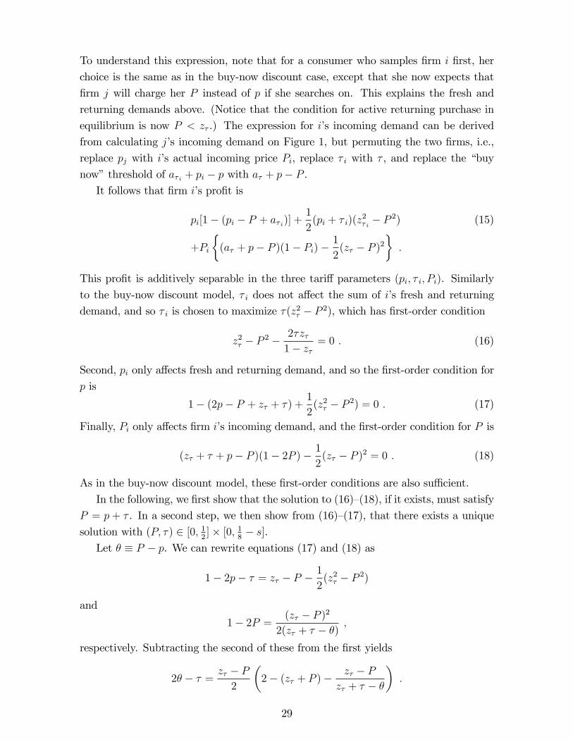
To understand this expression, note that for a consumer who samples �rm i �rst, her
choice is the same as in the buy-now discount case, except that she now expects that
�rm j will charge her P instead of p if she searches on. This explains the fresh and
returning demands above. (Notice that the condition for active returning purchase in
equilibrium is now P < z� .) The expression for i�s incoming demand can be derived
from calculating j�s incoming demand on Figure 1, but permuting the two �rms, i.e.,
replace pj with i�s actual incoming price Pi, replace � i with � , and replace the �buy
now�threshold of a� i + pi � p with a� + p� P .It follows that �rm i�s pro�t is
pi[1� (pi � P + a� i)] +1
2(pi + � i)(z
2� i� P 2) (15)
+Pi
�(a� + p� P )(1� Pi)�
1
2(z� � P )2
�:
This pro�t is additively separable in the three tari¤ parameters (pi; � i; Pi). Similarly
to the buy-now discount model, � i does not a¤ect the sum of i�s fresh and returning
demand, and so � i is chosen to maximize �(z2� � P 2), which has �rst-order condition
z2� � P 2 �2�z�1� z�
= 0 : (16)
Second, pi only a¤ects fresh and returning demand, and so the �rst-order condition for
p is
1� (2p� P + z� + �) +1
2(z2� � P 2) = 0 : (17)
Finally, Pi only a¤ects �rm i�s incoming demand, and the �rst-order condition for P is
(z� + � + p� P )(1� 2P )�1
2(z� � P )2 = 0 : (18)
As in the buy-now discount model, these �rst-order conditions are also su¢ cient.
In the following, we �rst show that the solution to (16)�(18), if it exists, must satisfy
P = p + � . In a second step, we then show from (16)�(17), that there exists a unique
solution with (P; �) 2 [0; 12]� [0; 1
8� s].
Let � � P � p. We can rewrite equations (17) and (18) as
1� 2p� � = z� � P �1
2(z2� � P 2)
and
1� 2P = (z� � P )22(z� + � � �)
;
respectively. Subtracting the second of these from the �rst yields
2� � � = z� � P2
�2� (z� + P )�
z� � Pz� + � � �
�:
29

Rewrite (16) as
� =1� z�z�
z2� � P 22
;
and subtracting it from the above equation yields
2(� � �) = z� � P2
�2� z� � P
z� + � � �� z� + P
z�
�=(z� � P )2(� � �)2z� (z� + � � �)
:
Hence, the solution if exists must satisfy � = �, i.e., P = p̂ = p+ � .
We now show existence and uniqueness. Let us focus on (16)�(17). First, we have
already shown that in equation (16) � decreases with P . Second, replace p in (17) by
P � � and then the two equations imply
P = 1� z� +�
1� z�;
which increases with � . Hence, the solution if exists must be unique. Substituting this
expression for P into (16) yields
z2� ��1� z� +
�
1� z�
�2=2�z�1� z�
:
If � = 0, then z� = 1�p2s � 1
2since s � 1
8. So the left-hand side is positive, greater
than the right-hand side which is zero. If � = 18� s, then z� = 1
2. So the left-hand side
is negative, less than the right-hand side which is positive. Hence, this equation has a
solution � 2 [0; 18� s]. Finally, given that � belongs to this interval, it follows from (16)
that P � 12.
References
Acquisti, A., and H. Varian (2005): �Conditioning Prices on Purchase History,�
Marketing Science, 24(3), 1�15.
Anderson, S., and R. Renault (1999): �Pricing, Product Diversity, and Search
Costs: A Bertrand-Chamberlin-Diamond Model,� RAND Journal of Economics,
30(4), 719�735.
Arbatskaya, M. (2007): �Ordered Search,�Rand Journal of Economics, 38(1), 119�
126.
Armstrong, M., and J. Vickers (2010): �Competitive Nonlinear Pricing and
Bundling,�Review of Economic Studies, 77(1), 30�60.
Armstrong, M., J. Vickers, and J. Zhou (2009): �Prominence and Consumer
Search,�Rand Journal of Economics, 40(2), 209�233.
30

Chen, Y. (1997): �Paying Customers to Switch,�Journal of Economics and Manage-
ment Strategy, 6(4), 877�897.
Chu, W., E. Gerstner, and J. Hess (1995): �Costs and Bene�ts of Hard-Sell,�
Journal of Marketing Research, 32(1), 97�102.
Daughety, A., and J. Reinganum (1992): �Search Equilibrium with Endogenous
Recall,�Rand Journal of Economics, 23(2), 184�202.
De los Santos, B. (2008): �Consumer Search on the Internet,�NET Institute Work-
ing Paper 08-15.
Deck, C., and B. Wilson (2006): �Tracking Customer Search to Price Discriminate,�
Economic Inquiry, 44(2), 280�295.
Diamond, P. (1971): �A Model of Price Adjustment,�Journal of Economic Theory,
3, 156�168.
Ellison, G., and A. Wolitzky (2008): �A Search Cost Model of Obfuscation,�
mimeo, MIT.
Fudenberg, D., and J. Tirole (2000): �Customer Poaching and Brand Switching,�
Rand Journal of Economics, 31(4), 634�657.
Gal-Or, E., M. Gal-Or, and A. Dukes (2007): �Optimal Information Revelation
in Procurement Schemes,�Rand Journal of Economics, 38(2), 400�418.
Hart, O., and J. Tirole (1988): �Contract Renegotiation and Coasian Dynamics,�
Review of Economic Studies, 55(1), 509�540.
Janssen, M., and A. Parakhonyak (2008): �Consumer Search with Costly Recall,�
mimeo.
Noe, T., and J. Wang (2004): �Fooling All the People Some of the Time: A Theory of
Endongenous Sequencing in Con�dential Negotiations,�Review of Economic Studies,
71(3), 855�881.
Reynolds, S., and J. Wooders (2009): �Auctions with a Buy Price,�Economic
Theory, 38(1), 9�39.
Roth, A., and X. Xing (1994): �Jumping the Gun: Inperfections and Institutions
Related to the Timing of Market Transactions,�American Economic Review, 84(4),
992�1044.
Vishwanath, T. (1989): �Job Search, Stigma E¤ects, and Escape Rate from Unem-
ployment,�Journal of Labor Economics, 7(4), 487�502.
31
Wolinsky, A. (1986): �True Monopolistic Competition as a Result of Imperfect In-
formation,�Quarterly Journal of Economics, 101(3), 493�511.
32