Comparisons of Performance between Quantum and Classical ...

SMU Data Science Review

Volume 1 | Number 4 Article 11

2018

Comparisons of Performance between Quantumand Classical Machine LearningChristopher HavensteinSouthern Methodist University, [email protected]

Damarcus ThomasSouthern Methodist University, [email protected]

Swami [email protected]

Follow this and additional works at: https://scholar.smu.edu/datasciencereview

Part of the Categorical Data Analysis Commons, Other Computer Sciences Commons, and theQuantum Physics Commons

This Article is brought to you for free and open access by SMU Scholar. It has been accepted for inclusion in SMU Data Science Review by anauthorized administrator of SMU Scholar. For more information, please visit http://digitalrepository.smu.edu.

Recommended CitationHavenstein, Christopher; Thomas, Damarcus; and Chandrasekaran, Swami (2018) "Comparisons of Performance between Quantumand Classical Machine Learning," SMU Data Science Review: Vol. 1 : No. 4 , Article 11.Available at: https://scholar.smu.edu/datasciencereview/vol1/iss4/11

https://scholar.smu.edu/datasciencereview?utm_source=scholar.smu.edu%2Fdatasciencereview%2Fvol1%2Fiss4%2F11&utm_medium=PDF&utm_campaign=PDFCoverPages

https://scholar.smu.edu/datasciencereview/vol1?utm_source=scholar.smu.edu%2Fdatasciencereview%2Fvol1%2Fiss4%2F11&utm_medium=PDF&utm_campaign=PDFCoverPages

https://scholar.smu.edu/datasciencereview/vol1/iss4?utm_source=scholar.smu.edu%2Fdatasciencereview%2Fvol1%2Fiss4%2F11&utm_medium=PDF&utm_campaign=PDFCoverPages

https://scholar.smu.edu/datasciencereview/vol1/iss4/11?utm_source=scholar.smu.edu%2Fdatasciencereview%2Fvol1%2Fiss4%2F11&utm_medium=PDF&utm_campaign=PDFCoverPages

https://scholar.smu.edu/datasciencereview?utm_source=scholar.smu.edu%2Fdatasciencereview%2Fvol1%2Fiss4%2F11&utm_medium=PDF&utm_campaign=PDFCoverPages

http://network.bepress.com/hgg/discipline/817?utm_source=scholar.smu.edu%2Fdatasciencereview%2Fvol1%2Fiss4%2F11&utm_medium=PDF&utm_campaign=PDFCoverPages



https://scholar.smu.edu/datasciencereview/vol1/iss4/11?utm_source=scholar.smu.edu%2Fdatasciencereview%2Fvol1%2Fiss4%2F11&utm_medium=PDF&utm_campaign=PDFCoverPages

http://digitalrepository.smu.edu

Comparisons of Performance between Quantumand Classical Machine Learning

Christopher L. Havenstein1, Damarcus T. Thomas1, andSwami Chandrasekaran2

1 Master of Science in Data Science, Southern Methodist University,Dallas, TX 75275 USA

2 Managing Director, Innovation & Enterprise Solutions,KPMG

{chavenstein, dtthomas}@[email protected]

Abstract. In this paper, we present a performance comparison of ma-chine learning algorithms executed on traditional and quantum comput-ers. Quantum computing has potential of achieving incredible results forcertain types of problems [1], and we explore if it can be applied to ma-chine learning. First, we identified quantum machine learning algorithmswith reproducible code and had classical machine learning counterparts.Then, we found relevant data sets with which we tested the compara-ble quantum and classical machine learning algorithms performance. Weevaluated performance with algorithm execution time and accuracy. Wefound that quantum variational support vector machines in some caseshad higher accuracy than classical support vector machines on multi-class classification problems. The main conclusion was that quantummulti-class SVM classifiers have the potential to be useful in the futureas quantum computer's available number of qubits increases.

1 Introduction

Quantum computing is an area of computing touted with achieving incredibleresults for factoring and unordered search problems [1]. Due to a phenomenoncalled quantum parallelism, which occurs because of superposition, quadratic orexponential increases in solution speed are possible with quantum computerswhen compared with classical computers [1]. However, quantum computing doesnot provide such a speedup for all problems and researchers are still learning inwhat situations it is best applied. The question we have is when quantum com-puting is combined with machine learning, do we still see these solution speedupsor perhaps does the machine learning solution accuracy increase? Researchershave already shown that quantum computing and machine learning can be com-bined. Through the concept of quantum parallelism, quantum computing canbe combined with machine learning when the machine learning algorithm canbe sufficiently parallelized [2]. The problem we are trying to solve is how doesquantum machine learning compare to classical machine learning and can theirrelative performance be measured?

1

Havenstein et al.: Quantum and Classical Machine Learning Performance Comparisons

Published by SMU Scholar, 2018

First, to solve this problem, we have performed a thorough search of availablequantum machine learning algorithms in research literature with reproduciblecode. Next, we required that the quantum machine learning algorithm to have acomparable classical machine learning algorithm available for comparison. Onceidentifying reproducible code to apply quantum machine learning algorithms, weidentified data sets which would be suitable for the type of quantum machinelearning algorithm—regression or classification. Through this process, we wereintroduced to quantum support vector machine (SVM) algorithms by a paper on“quantum enhanced feature spaces” that are applicable for classification machinelearning problems [3].

Second, solving our problem required access to a quantum computer to runquantum machine learning algorithms on. We were introduced to the IBM®Quantum Experience [4], which can be combined with IBM® application pro-gramming interfaces (APIs) to interact with quantum computers. This IBM®Quantum Experience allows a user to make an account, be granted an APIkey, and an allotment of credits to use. This API key uniquely identifies a userand their available credits to access quantum compute. Through IBM® QiskitAqua API, quantum machine learning algorithms were available to be used onIBM® quantum computers [5]. Last, to compare quantum and classical machinelearning algorithm performance, we decided on evaluation metrics to evaluatetheir relative performance. To determine if there was a quantum speedup overthe relevant classical machine learning algorithm, we utilized wall time, whichmeasures the program execution time on the classical or quantum hardware inmicroseconds. We additionally used accuracy as an evaluation metric to find therelative algorithm performance on the data sets selected.

Then, to describe our main results, an overview of our experiments are pro-vided. Through our experiments, we compared two types of quantum SVMseach against a classical SVM. For the quantum SVMs compared, a kernel-basedSVM and a variational SVM were both independently compared to a classicalSVM for a binary classification problem. Then, we compared the quantum vari-ational SVM to a classical SVM for a multi-class classification problem withthree classes. We found that for binary classification problems, there was nosignificant improvement over the classical SVM. However, for the multi-classclassification problem, the quantum variational SVM had higher accuracy thanthe classical SVM. Our main conclusions were that quantum variational SVMsperformed better in our experiments than classical SVMs for multi-class classi-fication problems. However, we observed no quantum speedups when comparingwall times for algorithm executions. We also experienced long queuing timesbefore we could run our quantum algorithms on an IBM® quantum computer.

This paper is structured in a way to provide the reader with relevant back-ground information and intuition to understand the key concepts. We beginby providing a conceptual overview of classical computing and machine learn-ing algorithms—focused on areas that are relevant to quantum computing. Anoverview of quantum machine learning follows, concluding with a summary onwhen quantum machine learning should be considered for use and when it should

2

SMU Data Science Review, Vol. 1 [2018], No. 4, Art. 11

https://scholar.smu.edu/datasciencereview/vol1/iss4/11

not. Next, descriptions of the binary classification data set and the multi-classclassification data set follow. Subsequently, the methods used and experimentsthat were performed are defined. After providing the methods and experiments,the results of our experiments are given in more detail. After providing an anal-ysis of the experiments, a descriptive analysis of the results is delivered. Theauthors then key ethical issues and relevant ethical principles are explored. Last,the authors supply their conclusions.

2 Classical Computing and Machine Learning

In classical computing, at the lowest level, data is stored with bits. Bits can takeon only one of two possible values based on whether an electron charge exists[6]. If no electron charge exists, the value of a bit is 0. Whereas, if there is anelectron charge, the value of a bit is 1. A sequence of bits is known as a bitstream[7]. Bitstreams store information which can be later analyzed. Table 1 on thenext page shows a sampling of different configurations of bits. It should also benoted as an aside that one letter can be stored in a byte [8].

Table 1. Bit configurations

Number of bits Example Name

1 0 Bit4 0, 1, 0, 0 Nibble8 0, 0, 1, 1, 0, 0, 1, 0 Byte

One or more input bitstreams are operated on by using logic gates. TheOxford Dictionary of Computing states that a logic gate is “a device, usuallybut not exclusively electronic, that implements an elementary logic function;examples include AND, OR, NAND, and NOR gates, and inverters [9].” Logicgates tend to make more sense when shown pictorially. Please view table 2 forexamples of input bit values and their output value after passing through variouslogic gates. Please note that table two spans across two pages. We created thistable after learning concepts found in [10].

Next, bitstreams can be processed in serial or parallel. In serial processing,only one input bitstream can be processed at a given time to generate output.Please refer to figure 1 for a pictorial example of serial processing.

Next, parallel processing can utilize multiple input bitstreams to generatemultiple outputs at a given time, which is a crucial distinction when evaluat-ing machine learning within quantum computing. Please refer to figure 2 for apictorial example of parallel processing. Later, in the quantum computing andmachine learning section, we discuss why parallel processing is more importantthan serial processing for quantum computers.

3



Table 2. Logic gate examples

Type of logic gate Logic gate diagram Table representation

And gate

Input 1 Input 2 Output

0 0 01 0 00 1 01 1 1

Or gate


0 0 01 0 10 1 11 1 1

XOR gate


0 0 01 0 10 1 11 1 0

Fig. 1. A simple figure illustrating serial processing. Notice an input bitstreamfeeds into a “black box” which abstracts a series of logic gates or other processing.Then, a bit is output from the black box.

4



Fig. 2. A simple figure illustrating parallel processing. Notice there are four inputbitstreams that feed into a “black box” which abstracts a series of logic gates orother processing. Then, two bits are output from the black box simultaneously.

Thankfully, we can abstract these concepts generally and not be botheredwith them. However, they will later become relevant when describing quantumcomputing and how it pertains to machine learning. Though, we do have someexamples of machine learning algorithms that do have components that are sim-ilar to logic gates. One such example are activation functions in neural networks.We do not expect the reader to fully understand neural networks. Conceptually,the activation function takes a series of weighted inputs to produce an outputwithin a range defined by the type of activation function. There are various typesof activation functions, but one example is a sigmoid function that restricts theoutput to either a 0 or 1. An example of a neural network is provided in figure3.

As we alluded to, it is more typical in machine learning to think at an algo-rithmic level. Algorithms generally are comprised of a series of steps and mayhave iteration [11] and/or recursion [12]. In algorithms, the order of these steps isimperative, and sometimes the algorithm will not work if the steps are performedin the wrong order. Algorithms can be implemented using serial or parallel pro-cessing. However, a serial algorithm may not work well or at all in parallel. Thereverse is also possible.

Machine learning algorithms are broadly described as applicable to classifi-cation or regression problems. First, we begin describing classification problems.In classification problems, the objective for the machine learning algorithm is totrain a classifier to predict a label of a class. To do this, the machine learningalgorithm learns from patterns in the distribution of the data for input variables,also known as features. The label being predicted, also known as a target, mustbe provided for training purposes. Overall, the data used to train a machinelearning algorithm is called training data. Then, the classifier uses the input fea-

5



Fig. 3. A figure of a neural network architecture. Activation functions are similarto logic gates since they take a number of inputs to generate outputs.

tures for new unseen data, known as test data, to predict an unknown label. Forinstance, the classifier would be trained to predict given input features to predictthe target label of “this” or “that” (binary classification), or perhaps “this” or“that” or “the other thing” and etc. (which is multi-class classification). Second,for regression machine learning problems, we still have training and test dataand input features, but the predicted target is a real number—often known as acontinuous value.

In this paper, we do not explore all of the available classification and regres-sion machine learning algorithms that are usable on a classical computer. Re-gardless, the reader should be aware that machine learning algorithms typicallyfall into one of these two categories. Next, an overview of quantum computingand the concepts relevant to quantum machine learning is presented.

3 Quantum Computing and Machine Learning

Quantum computers look much different in person than the computers we useevery day. The writers believe quantum computers look similar to metal chan-deliers. For copyright purposes, we cannot provide a picture of a quantum com-puter in-line, but the writers suggest that you refer to the link in [13]. Toparaphrase IBM® Research division, quantum computers require an extremelycold environment and containment from outside “electromagnetic radiation” toguard against the introduction of error into the quantum processing chip [13].The quantum processing chip must be kept at “[approximately] -459.67 degreesFahrenheit”, according to IBM® [13].

While classical computers operate on bitstreams where each bit can take onone of two values each (0 or 1), quantum computers have quantum bits with

6



unique properties. First, we describe quantum bits, which are most commonlyknown as qubits. Qubits can be in multiple states at once, which can be easiestexplained as spinning in the electron. If the electron spin is in the “up” position,then the qubit would equal 1 [14]. Whereas, if the electron spin were in thedown position, the qubit would equal 0 [14]. However, in quantum computing,we have no way of knowing at a given time whether the qubit is in the up ordown position. Therefore, a superposition (i.e. a sphere) of all potential valuesis created [14]. To compare bits to qubits visually, please refer to figure 4. Thesphere created by the spinning of the qubit is commonly known in quantumcomputing as a “Bloch sphere [14].”

Fig. 4. A figure of a qubit. The notation used for the 1 and 0 values comes fromDirac, and is known as a “ket [14].” A series of qubit values are notated within aket. The red arrows represent the spinning of the qubit, which creates a spherepattern. This spinning represents the superposition of values available to thequbit.

In quantum computing, we still use logic gates, but the logic gates havedifferent purposes. Quantum logic gates are commonly known as quantum gates,and they are essentially a transformation on one or more qubits. In table 3, wehave provided a sample of quantum gate types from [15].

Table 3. Quantum gate examples

Quantum gate Input Classical gate Short description

Hadamard gate 1 qubit None Creates superpositionPauli-X gate 1 qubit Not gate Creates x rotationPauli-Y gate 1 qubit None Creates y rotation

Controlled not gate 2 or more qubits Not gate Used to measure 2nd qubit

For this paper, the reader does not need to become intimately familiar withquantum gates. However, the reader should know quantum gates are impor-

7



tant because they transform input qubits with transformations. These quantumtransformations include but are not limited to establishing the quantum state(e.g., superposition) and to measure qubits (e.g., with the CNOT gate) [15].However, if the reader would like a more in-depth mathematical explanation ofquantum gates, please refer to [16].

Quantum computing becomes much more interesting when multiple qubitsare entangled together [16]. In [16], entanglement is described as having “deepconnections between spatially separated entities.” When qubits are entangled,the superposition of values also increases. When some qubits, n, are entangled,the superposition of values is 2n [16]. For two entangled qubits, we have repre-sented the available values in the superposition in figure 5.

Fig. 5. A figure of a two entangled qubits. Notice that there are four uniquevalues in the superposition of values.

At this juncture, the reader may intuit that a large number of qubits entan-gled leads to a large superposition of values available to perform operations on aquantum computer. At the authors time of writing this paper, IBM® currentlyhas 5 qubit (“IBM® Q 5 Tenerife”), 14 qubit (“IBM® Q 14 Melbourn”), and16 qubit (“IBM® Q 16 Rschlikon”) quantum computers available for public use[17]. Also, IBM® has a 20 qubit quantum computer available for private use(“IBM® Q 20 Tokyo”) [17]. Current quantum computing researchers in [16]suggest that the current highest performance supercomputers are only able torepresent the superposition of values in a quantum computer up to 50 qubits.At 50 qubits, the superposition of values available to the quantum computer ata given time would be 1,125,899,906,842,624, or 250.

Regarding machine learning, it is beneficial to know the circumstances ofwhen a quantum computer should be used. When a machine learning algorithmcan be parallelized, “quantum parallelism” may be possible to apply, accordingto [2]. According to [18], when you have a quantum computer with large super-

8



position of values due to many entangled qubits, you can measure the functionoutput for many values simultaneously. However, for a serial machine learningalgorithm, a quantum computer's large superposition of values is wasted, sinceonly a small portion of the superposition is utilized.

To reinforce the idea of when machine learning may be able to be appliedon a quantum computer, we provide a conceptual example of a good potentialquantum machine learning algorithm candidate. Random Forests are a type ofmachine learning algorithm that can be run in parallel and may make a goodquantum machine learning algorithm. Leo Breiman introduced the random forestmachine learning algorithm in his 2001 paper, which can be used for classificationor regression problems [19]. For Random Forests, the overall data set (as inmost machine learning algorithms) is broken into a training and test data set.However, from the training data set, approximately one third is set aside asan “out of bag” set. The out of bag set is used to evaluate the performance ofthe Random Forest model created from the training data set. Random Forestsutilize “bagging” which is short for bootstrap aggregating, and we describe next[19]. Then, the n bootstrap samples are selected from the training data withreplacement to create trees in the random forest. With replacement means thatonce an observation is selected, it is put back into the pool to be potentiallysampled again. Then, for each bootstrapped sample, the process of creatinga tree begins. For each bootstrap sample with a predetermined sample size,a random feature (e.g. a variable) is chosen to create a binary split from thetraining data [19]. This process of creating random binary splits continues untila user-defined maximum tree depth is reached. After all n trees are created inthis way (which can be in parallel), the tree results are aggregated together tocreate the fitted random forest model. These aggregations generally are votes forclassification problems and averages for regression problems. The fitted randomforest model then predicts the target variable from the out of bag set to reportthe training error. Then, the model can be used to predict the target on the testdata set. An example of a Random Forest is provided in figure 6.

While a Random Forest is a good potential candidate for a quantum ma-chine learning algorithm, a Boosted Trees model is a bad example of a quantummachine learning algorithm. This is because boosted trees are fit in serial. XG-Boost is a type of Boosted Trees machine learning algorithm that is currentlyheavily used on classical computers [21]. Without going into as much depth aswith Random Forest models, Boosted Tree models are required to fit a series oftrees. After each tree is fit, the prediction errors are up-weighted and the correctpredictions are down-weighted. Then, the next tree is fit after incorporating thenew weights. This process continues until a number of trees are fit. Then, theresults are aggregated together and weighted by the trees that had the best in-dividual tree accuracy. An example of part of the boosted tree fitting process isprovided in figure 7.

In summary, quantum machine learning should be considered when a partic-ular machine learning algorithm candidate can be parallelized—to benefit fromquantum parallelism. However, serial machine learning algorithms should be kept

9



Fig. 6. A figure showing the Random Forest algorithm fitting process.

Fig. 7. A figure showing the Boosted Trees algorithm fitting process.

10



on a classical computer. Next, we began searching for viable quantum machinelearning algorithms. We found that there was a common algorithm used as afoundation for many of these quantum machine learning algorithms, Grover'sSearch. Grover's Search is a quantum algorithm that has been shown to be use-ful for clustering, Support Vector Machines, and Quantum Neural Networks [1].For data that is in unordered sets, Grover's Search can find a globally optimumvalue extremely quickly and has been shown very valuable for machine learning[20]. For quantum clustering problems, Grover's Search is used almost exclusively[21].

The following observation we made is that many of the types of quantummachine learning algorithms found in our literary review did not have repro-ducible code that we could find. We considered this a serious issue. There wasonly one type of quantum machine learning algorithm with reproducible codethat we found, for quantum support vector machines. In table 4, we provide:(1) the types of quantum machine learning algorithms we found; (2) the type ofmachine learning problem the algorithm can be applied to; and (3) the citationsfound. We were only able to find reproducible code for quantum support vectormachines. At this point, we proceed to our descriptions of the data sets used tosolve our problem.

Table 4. Quantum machine learning algorithms found through literary review

Quantum ML algorithm Applicable ML problems Citations

Quantum annealing Regression [1], [22], [23]Quantum adiabatic algorithms Classification [24], [25], [26]Quantum neural networks Regression or Classification [27]Quantum process tomography Regression [1], [28]Quantum support vector machines Classification [3]

4 Data Sets

There were two data sets used to solve our problem. The first data set thatwas chosen is the UCI ML Breast Cancer Wisconsin (Diagnosis) data set thatis available from scikit learn [29]. Features are computed from a digitized imageof a fine needle aspirate (FNA) of a breast mass. They describe characteristicsof the cell nuclei present in the image. This data set has 569 observations with30 columns that are used as features to predict the diagnosis value of a benignbreast cancer cell nuclei, 1. The default diagnosis value, 0, indicates that a breastcancer cell nuclei is malignant. The breast cancer data set is suitable for quantummachine learning algorithms that solve supervised binary classification problems.For more in-depth explanation of the columns and their values in the breastcancer data set, please refer to Appendix I: Data Set Descriptions. The quoted

11



column descriptions in the breast cancer data dictionary came from a Kaggleentry for the breast cancer data set [29].

The second data set that was chosen is the UCI ML Wine data set. Thefeatures are the results of a chemical analysis of wines grown in the same regionin Italy but derived from three different cultivars. The analysis determined thequantities of 13 constituents found in each of the three types of wines [30]. Thedata set has 178 observations and the class identifier are 1, 2, 3. For more indepth explanation of the columns and their values in the wine data set, pleaserefer to Appendix I: Data Set Descriptions. The quoted column descriptions inthe breast cancer data dictionary came from the UCI data repository. The Winedata set is suitable for multi-classification quantum machine learning algorithms.

5 Methods and Experiments

We utilized Qiskit Aqua for quantum machine learning. We used both a lo-cal quantum computer simulator and a real quantum chip as our backend. Weapplied two quantum machine learning algorithms, Support Vector Machine'svariational method and the Support Vector Machine's quantum kernel-basedmethod for supervised classification. The direct kernel-based method for SVMwas run on a classical computer that utilized a regular CPU.

We used the methods discovered by Vojtech Havlicek et al. [3] to apply twoquantum machine learning methods to classification problems. We have appliedtwo quantum support vector machine learning methods for binary classificationproblems, using the breast cancer data set. These two methods are the quantumvariational method and the quantum kernel-based method.

In [3], the authors suggest that their quantum support vector machine algo-rithms could be applied in the near future on quantum architectures. They haveeven provided an example Jupyter notebook to show how one of their algorithmsworks [31]. We utilized their Jupyter notebook as a baseline for this analysis,since the reader will likely have the aptitude to apply quantum machine learn-ing in Python with such a Jupyter notebook—after downloading the requiredpackage libraries. The authors in [3] state that their methods were run on aquantum computer, but they have not shown this in their Jupyter notebook.Since, their code in their notebook is rerunning with a local quantum simula-tor in Qiskit Aqua. Next, we describe the quantum variational method and thequantum kernel-based method, beginning with the quantum variational method.

With the quantum variational method, hyperplane(s) are calculated and usedfor classification of new test data. In the simplest sense, if the training data areused and plotted in two dimensions, similar to a scatterplot, a hyperplane isthe line (or curve in higher dimensions) that separates the class values that thetraining data belongs to (often denoted as the yi values). The main advantage ofthe quantum variational method is that it can handle classification of more thantwo classes for the response variable. The disadvantage of the quantum varia-tional method is that it requires two sequential quantum algorithms to be run,which is much more computationally intensive than the quantum kernel-based

12



method. The first algorithm is used when trying to compute the hyperplane(s)with the training data. This first algorithm can be found in figure 8. The secondalgorithm runs after the hyperplane(s) from the first algorithm are calculatedand are used to begin classifying the new test data. You can find the secondalgorithm in figure 9 [3].

Fig. 8. A figure showing the first algorithm in the quantum variational SVMmethod. This algorithm was found in [3].

The second quantum support vector method, is the quantum kernel-basedmethod, is restricted to only binary classification problems. However, it is muchquicker to complete since the quantum computer is only used for one algorithm.Whereas, the quantum variational method has to run two algorithms, one tocalculate the hyperplane(s) and another to classify the test data. Accordingto the authors of [32], the kernel approach used by the quantum kernel-basedmethod “cannot be estimated classically.” They also mention in their paper,that there won't be an advantage to using quantum kernel-based Support VectorMachines (SVM) if the data are not already complex to fit on classical silicon-based computers.

The steps for the quantum kernel-based SVM algorithm follow. As statedpreviously, with the quantum kernel-based method, we are restricted to onlyhaving two labels to classify (e.g. binary classification). The authors stated in [3]that it is technically possible to classify more than two labels, but partitioningwould have to occur into two label sets, and the developer would require a deeperunderstanding of quantum hardware. First, a kernel matrix is estimated withthe quantum computer by using all of the training data rows. Then, the classicalcomputer takes this quantum kernel matrix of the training data to calculate

13



Fig. 9. A figure showing the first algorithm in the quantum variational supportvector machine method. This algorithm was found in [3].

the support vectors with the classical computer. After the support vectors arecalculated with the classical computer, classification can begin by the classicalcomputer to predict the labels for the test data set. Because the support vectorswere already calculated and the quantum kernel matrix from the training datais available, the label can be directly calculated for each of the test data rows.

The classical support vector machine method used for comparative purposesis the “Support Vector Machine Radial Basis Function Kernel (SVM RBF Ker-nel)” which is made available in Qiskit Aqua and is briefly described in theirdocumentation [32].

For our experiments, we used code from our Jupyter Notebook which canbe found in Appendix II: Python Code from Quantum SVM Analysis JupyterNotebook. Table 5 lists out the complete experimental configurations. Pleasenote that the runtime and accuracy percentage will be compared amongst thetwo different algorithms. We also utilized four different types of back-ends, whichwere: (1) the local CPU; (2) the quantum simulator; (3) the state vector simu-lator; and (4) a real quantum chip. In the first approach, we use a variationalcircuit as given in [33] [34] that generates a separating hyperplane in the quan-tum feature space. In the second approach, we use the quantum computer toestimate the kernel function of the quantum feature space directly and imple-ment a conventional SVM.

6 Analysis

After deciding on how to setup the experiments, we began the analysis. We triedapplying the quantum variational SVM model to the same training and test splitfor the breast cancer data set (with 20 training and 10 test observations). Asexpected, this model took too long to fit, with a total approximate run timeof 25 minutes. However, the accuracy when we use the quantum simulator forthe quantum variational SVM model completed was 95%, as we show in Table6. The classic SVM had a slower wall time with only an 85% accuracy. The

14



Table 5. Experimental setup configurations

Algorithmcompared

Quantum orclassical

Back-end Runtime Data setEvaluationmetric

Kernel-basedSVM

QuantumQuantumback-end(ibmqx4)

Wall time(µs)

UCI BreastCancerWisconsin

Accuracy

Kernel-basedSVM

QuantumQuantumsimulator

Wall time(µs)


Accuracy

Kernel-basedSVM

QuantumStatevectorsimulator

Wall time(µs)


Accuracy

Classic SVM ClassicalLocal CPUenvironment

Wall time(µs)


Accuracy

VariationalSVM


Wall time(µs)


Accuracy

Variational(multi-class)SVM

QuantumQuantumback-end(ibmqx4)

Wall time(µs)

Wine Accuracy



Wall time(µs)

Wine Accuracy


ClassicalLocal CPUenvironment

Wall time(µs)

Wine Accuracy

15



simulated variational model outperformed the local CPU as it should have sincesuch variational circuit classifiers are directly related to conventional SVMs [35].

Table 6. Quantum variational SVM results on the Breast Cancer Wisconsindata set

Classifiers Back-end Algorithm Wall Time Accuracy

QuantumSVM

Quantumsimulator

VariationalSVM

5.96 µs 95.00%

Classic SVMLocal CPUenvironment

SVM 6.20 µs 85.00%

Next, as our control, we applied the classical “Support Vector Machine RadialBasis Function Kernel (SVM RBF Kernel)” to the same training and test splitfor the breast cancer data set (with 20 training and 10 test observations) [32].Table 7 summarizes the kernel-based binary classification results. The quantumstate vector simulator had 100% accuracy in approximately 6 microseconds. Theclassic SVM run on a local CPU had 85% accuracy.

Table 7. Quantum kernel-based SVM results on the Breast Cancer Wisconsindata set


QuantumSVM

ibmqx4SVM RBFKernel

6.91 µs 80.00%

QuantumSVM

Statevectorsimulator

SVM RBFKernel

5.96 µs 100.00%


SVM 6.20 µs 85.00%

We ran the classical SVM RBF Kernel model a few more times, and receivedthe same result, of 85% prediction accuracy each time. It was after this werealized that the quantum SVM methods appeared to have more variabilityduring the model fit process than the classical SVM model did. We were also

16



impressed with how easy it was after running through one example dataset to fitquantum machine learning models. On multi-class variational SVM comparisonsas noted in Table 8, the quantum simulator had the best accuracy (100%). Thequantum SVM run on a quantum chip had an accuracy of 93%. The local CPUSVM had 90% accuracy.

Table 8. Quantum multi-class variational SVM results on the Wine data set


QuantumMulti-classSVM

ibmqx4VariationalSVM

6.44 µs 93.33%

QuantumMulti-classSVM

Statevectorsimulator

VariationalSVM

5.96 µs 100.00%


SVM 6.20 µs 90.00%

7 Results

The results on the Breast Cancer Wisconsin data set are reviewed first. On theBreast Cancer Wisconsin data set, only simulator results were obtained for thequantum variational SVM while quantum computer results were obtained forthe quantum kernel-based SVM. The quantum variational SVM results werenot obtained after waiting for approximately a day for the results to return.It was unclear if this wait was due to queuing issues or the run time of thequantum variational SVM on the IBM® quantum computer. For the quantumvariational SVM simulator results, the accuracy was 95.00% when compared to85.00% with the classical SVM to predict benign or malignant breast cancertumors. For the quantum kernel-based SVM, the best results were obtained bythe quantum SVM simulator with 100.00% accuracy. The classical SVM hadthe next highest accuracy at 85.00%. Then last, the quantum kernel-based SVMrun on a quantum computer performed the worst with 80.00% accuracy on theBreast Cancer Wisconsin data set.

The results for the Wine data set are reviewed next. The quantum multi-class variational SVM run on the simulator had the best accuracy at 100.00% topredict the three types of wine. Next, the quantum multi-class variational SVMrun on the quantum computer had 93.33% accuracy. Last, the classic SVM had90.00% accuracy on the Wine data set.

17



There were a few key insights gained after reviewing these results on bothdata sets. First, fitting quantum SVM models on large data sets for binaryclassification problems appeared initially to be computationally inefficient. Theauthors believe that using 20 training and 10 test observations isn’t enough forpractical use, and is primarily useful only as a proof of concept. The authorswould like to see if the performance improves with a quantum computer withmore qubits. The authors will also state that the most likely explanation for longruntime of the SVMs on IBM® quantum computers was due to long queuingtimes. The justification for this statement is due to the low wall-times (measuredin microseconds) returned from the quantum computer, while the overall runtimewas typically long (greater than 20 minutes).

Second, the difference in predictive accuracy between the simulated quantumSVM and the actual quantum SVM suggests that the simulator tends to overstatethe accuracy of quantum SVMs run on quantum computers.

Finally, The most interesting results were found from the quantum variationalSVM to perform multi-class classification on the Wine Data Set. Since, thequantum variational SVM for the multi-class classification problem had higheraccuracy than the classical SVM (93.33% compared to 90.00%).

8 Ethics

During our analysis, we discovered a potential ethical issue that we deemedworthy of discussion. Here, we provide some background to introduce the po-tential ethical issue. While the wall times we observed to fit the quantum SVMswere short—typically taking a few microseconds—the queuing times were longin comparison. We do acknowledge that in our python code we initially did notthink to include a runtime timer in addition to the wall time timer. If we did,we would have recorded from our experiences very long code run times. For thekernel-based quantum SVM on the Breast Cancer Wisconsin data set, the codeexecution time from running the line to receiving results back from the quan-tum computer was approximately 20 to 30 minutes. Then, with the variationalquantum SVM on the Wine data set, we received results back from the quantumcomputer in approximately 5 to 6 hours. This queueing time for the variationalSVM on the Wine multi-class classification data set was unfortunate since theresults were the most promising.

The experience of waiting in a slow queue to access the IBM® quantumcompute led us to wonder, what if clients were provided unequal access to thequantum computers queue? This is a potential ethical issue, which right nowdoesn't have much impact other than being an annoyance, but in the future couldbecome a serious ethical issue. We believe that access to quantum computersshouldn't be restricted.

As a framework to evaluate the ethical issue we are exploring—access toquantum computers shouldn't be restricted—we used two ethical principles. Thefirst ethical principle we used for evaluation of this ethical issue was beneficenceaccessed from the Stanford Encyclopedia of Philosophy [36]. Then, we used the

18



ethical principle Be fair and take action not to discriminate from the ACM codeof ethics [37].

Initially, we evaluated the ethical issue, access to quantum computers shouldnot be restricted, with the ethical principle “beneficence [36].” According to [36],the ethical principle of beneficence alludes to a moral obligation to provide someservice or to perform an action to help others. If IBM® intends to providea free quantum computing service, then that service should be provided withequal access to all requesting clients. If IBM® is not providing equal accessto their free quantum computing service, then beneficence is violated. Fromthe authors' perspective, IBM® is doing a great job with providing access toquantum compute currently. In the probable future where quantum computersbecome more impactful, we believe that IBM® should continue to provide thisfree quantum computing service for educational purposes.

Last, we evaluated this potential ethical issue with the ethical principle “Befair and take action not to discriminate [37].” This ethical principle is similar tobeneficence, but also focuses on equal treatment of all people. For IBM® not tobe discriminating with access to their free quantum compute, all clients wouldhave to be treated equally. To not violate this ethical principle, no discriminatingon clients on any basis can occur when requesting access with a valid API key tothe free IBM® quantum compute. If any discriminating or unequal treatmentoccurs where some clients are more equal than others, then the ACM ethicalprinciple “be fair and take action not to discriminate” is violated. We challengeIBM® in the future to keep comparable free access available to their quantumcomputers as is available now for educational purposes.

9 Conclusions and Future Work

Experimentally we have shown that a classifier can exploit a quantum featurespace. The kernel of this feature space has been conjectured to be hard to esti-mate classically. In the experiment we find that even in the presence of noise, weare capable of achieving success rates up to 93.00% with quantum compute. Inthe future it becomes intriguing to find suitable feature maps for this techniquewith provable quantum advantages while providing significant improvement onreal world data sets. With the ubiquity in machine learning, we are optimisticthat our technique will find application beyond with SVM classifiers. Two ma-jor issues should be addressed, for one, the quantum simulator was executedon a local classical machine. Despite the efforts of the backend, it is not feasi-ble for a classical computer to imitate a quantum computer without some typeof high-performance computing power, and so the simulator results are purelyobservational. Furthermore, the presence of noise diminishes the results on areal quantum chip especially with the limited number of qubits. Small quantumcomputers and larger special purpose quantum simulators, annealers, etc., ex-hibit promising applications in machine learning and data analysis [38]. Howeverwe are in a certain quantum era called, the Noisy Intermediate-Scale Quantum(NISQ) era. Here “intermediate scale” refers to the size of quantum computers

19



which will be available in the next few years. NISQ tends to refer to quantumcomputers having number of qubits ranging from 50 to a few hundred 50 qubitsas a significant milestone. This is because that's beyond what can be simulatedby brute force using the most powerful existing digital supercomputers. “Noisy”emphasizes that we will have imperfect control over those qubits; the noise willplace serious limitations on what quantum devices can achieve in the near term[39]. It is unknown whether the NISQ era will yield great developments andtechnologies that speed up the time to solutions. Nonetheless, we are living inexciting times where experimentation on real quantum chips are possible, and anew quantum community is developing and trickling over to the curiosity of thegeneral public minds.

References

1. Peter Wittek. Quantum machine learning: what quantum computing means to datamining. Academic Press, 2014.

2. Daoyi Dong, Chunlin Chen, Hanxiong Li, and Tzyh-Jong Tarn. Quantum rein-forcement learning. IEEE Transactions on Systems, Man, and Cybernetics, PartB (Cybernetics), 38(5):1207–1220, 2008.

3. Vojtech Havlicek, Antonio D Corcoles, Kristan Temme, Aram W Harrow, Jerry MChow, and Jay M Gambetta. Supervised learning with quantum enhanced featurespaces. arXiv preprint arXiv:1804.11326, 2018.

4. IBM Staff. Ibm quantum experience. https://quantumexperience.ng.bluemix.

net/qx/experience.5. IBM Staff. Quantum information science kit. https://qiskit.org/aqua.6. David Deutsch. Quantum theory, the church–turing principle and the universal

quantum computer. Proc. R. Soc. Lond. A, 400(1818):97–117, 1985.7. Community Editor. Bitstream. https://en.wikipedia.org/wiki/Bitstream.8. Ashley Taylor. Bits bytes. https://web.stanford.edu/class/cs101/

bits-bytes.html.9. Reference Staff. Logic gates quick reference. http://www.oxfordreference.com/

view/10.1093/oi/authority.20110810105307777.10. Margaret Rouse. logic gate (and, or, xor, not, nand, nor

and xnor). https://whatis.techtarget.com/definition/

logic-gate-AND-OR-XOR-NOT-NAND-NOR-and-XNOR.11. Reference Staff. Iteration. https://www.oxfordlearnersdictionaries.com/us/

definition/english/iteration.12. Chris Alvin. Recursive function. http://pages.cs.wisc.edu/~calvin/cs110/

RECURSION.html.13. IBM Staff. Inside look: Quantum computer. https://www.research.ibm.com/

ibm-q/learn/what-is-ibm-q/images/infographic-inside.jpg.14. Eleanor G Rieffel and Wolfgang H Polak. Quantum computing: A gentle introduc-

tion. MIT Press, 2011.15. Community Editor. Quantum logic gates. https://en.wikipedia.org/wiki/

Quantum_logic_gate.16. Krysta M Svore and Matthias Troyer. The quantum future of computation. Com-

puter, 49(9):21–30, 2016.17. IBM Staff. Quantum devices simulators. https://www.research.ibm.com/ibm-q/

technology/devices/.

20



https://quantumexperience.ng.bluemix.net/qx/experience

https://quantumexperience.ng.bluemix.net/qx/experience

https://qiskit.org/aqua

https://en.wikipedia.org/wiki/Bitstream

https://web.stanford.edu/class/cs101/bits-bytes.html

https://web.stanford.edu/class/cs101/bits-bytes.html

http://www.oxfordreference.com/view/10.1093/oi/authority.20110810105307777

http://www.oxfordreference.com/view/10.1093/oi/authority.20110810105307777

https://whatis.techtarget.com/definition/logic-gate-AND-OR-XOR-NOT-NAND-NOR-and-XNOR

https://whatis.techtarget.com/definition/logic-gate-AND-OR-XOR-NOT-NAND-NOR-and-XNOR

https://www.oxfordlearnersdictionaries.com/us/definition/english/iteration

https://www.oxfordlearnersdictionaries.com/us/definition/english/iteration

http://pages.cs.wisc.edu/~calvin/cs110/RECURSION.html

http://pages.cs.wisc.edu/~calvin/cs110/RECURSION.html

https://www.research.ibm.com/ibm-q/learn/what-is-ibm-q/images/infographic-inside.jpg

https://www.research.ibm.com/ibm-q/learn/what-is-ibm-q/images/infographic-inside.jpg

https://en.wikipedia.org/wiki/Quantum_logic_gate

https://en.wikipedia.org/wiki/Quantum_logic_gate

https://www.research.ibm.com/ibm-q/technology/devices/

https://www.research.ibm.com/ibm-q/technology/devices/

18. J. Lanzagorta, M. Uhlmann. Quantum parallel real? https:

//www.researchgate.net/profile/Marco_Lanzagorta/publication/

252477910_Is_quantum_parallelism_real/links/54982fc80cf2eeefc30f7e2c/

Is-quantum-parallelism-real.pdf.19. L. Breiman. Random forest. https://www.stat.berkeley.edu/~breiman/

randomforest2001.pdf.20. Christoph Durr and Peter Hoyer. A quantum algorithm for finding the minimum.

arXiv preprint quant-ph/9607014, 1996.21. Esma Aımeur, Gilles Brassard, and Sebastien Gambs. Quantum speed-up for un-

supervised learning. Machine Learning, 90(2):261–287, 2013.22. Emile HL Aarts et al. Simulated annealing: Theory and applications. 1987.23. AB Finnila, MA Gomez, C Sebenik, C Stenson, and JD Doll. Quantum annealing:

a new method for minimizing multidimensional functions. Chemical physics letters,219(5-6):343–348, 1994.

24. Hartmut Neven, Vasil S Denchev, Geordie Rose, and William G Macready. Train-ing a binary classifier with the quantum adiabatic algorithm. arXiv preprintarXiv:0811.0416, 2008.

25. Wim Van Dam, Michele Mosca, and Umesh Vazirani. How powerful is adiabaticquantum computation? In Foundations of Computer Science, 2001. Proceedings.42nd IEEE Symposium on, pages 279–287. IEEE, 2001.

26. David DiVincenzo. Quantum information processing. lecture notes.27. Sanjay Gupta and RKP Zia. Quantum neural networks. Journal of Computer and

System Sciences, 63(3):355–383, 2001.28. Isaac L Chuang and Michael A Nielsen. Prescription for experimental determina-

tion of the dynamics of a quantum black box. Journal of Modern Optics, 44(11-12):2455–2467, 1997.

29. Nick Street. Scikit learn dataset load. http://scikit-learn.org/stable/

modules/generated/sklearn.datasets.load_breast_cancer.html.30. Nick Street. Breast cancer wisconsin (diagnostic) data set. https://www.kaggle.

com/uciml/breast-cancer-wisconsin-data/version/2.31. Qiskit Community. Qiskit aqua-tutorials. https://github.com/Qiskit/

aqua-tutorials/blob/master/artificial_intelligence/svm_qkernel.ipynb.32. Qiskit Community. Support vector machine radial basis function kernel

svm rbf kernel. https://qiskit.org/documentation/aqua/algorithms.html#

support-vector-machine-radial-basis-function-kernel-svm-rbf-kernel.33. Abhinav Kandala, Antonio Mezzacapo, Kristan Temme, Maika Takita, Markus

Brink, Jerry M Chow, and Jay M Gambetta. Hardware-efficient variational quan-tum eigensolver for small molecules and quantum magnets. Nature, 549(7671):242,2017.

34. Edward Farhi, Jeffrey Goldstone, Sam Gutmann, and Hartmut Neven. Quantumalgorithms for fixed qubit architectures. arXiv preprint arXiv:1703.06199, 2017.

35. Christopher JC Burges. A tutorial on support vector machines for pattern recog-nition. Data mining and knowledge discovery, 2(2):121–167, 1998.

36. T Beauchamp. The principle of beneficence in applied ethics. https://plato.

stanford.edu/entries/principle-beneficence/.37. Committee Editor. Acm code of ethics. https://www.acm.org/code-of-ethics.38. Rodion Neigovzen, Jorge L Neves, Rudolf Sollacher, and Steffen J Glaser. Quantum

pattern recognition with liquid-state nuclear magnetic resonance. Physical ReviewA, 79(4):042321, 2009.

39. John Preskill. Quantum computing in the nisq era and beyond. arXiv preprintarXiv:1801.00862, 2018.

21



https://www.researchgate.net/profile/Marco_Lanzagorta/publication/252477910_Is_quantum_parallelism_real/links/54982fc80cf2eeefc30f7e2c/Is-quantum-parallelism-real.pdf




https://www.stat.berkeley.edu/~breiman/randomforest2001.pdf

https://www.stat.berkeley.edu/~breiman/randomforest2001.pdf

http://scikit-learn.org/stable/modules/generated/sklearn.datasets.load_breast_cancer.html

http://scikit-learn.org/stable/modules/generated/sklearn.datasets.load_breast_cancer.html

https://www.kaggle.com/uciml/breast-cancer-wisconsin-data/version/2

https://www.kaggle.com/uciml/breast-cancer-wisconsin-data/version/2

https://github.com/Qiskit/aqua-tutorials/blob/master/artificial_intelligence/svm_qkernel.ipynb

https://github.com/Qiskit/aqua-tutorials/blob/master/artificial_intelligence/svm_qkernel.ipynb

https://qiskit.org/documentation/aqua/algorithms.html#support-vector-machine-radial-basis-function-kernel-svm-rbf-kernel

https://qiskit.org/documentation/aqua/algorithms.html#support-vector-machine-radial-basis-function-kernel-svm-rbf-kernel

https://plato.stanford.edu/entries/principle-beneficence/

https://plato.stanford.edu/entries/principle-beneficence/

https://www.acm.org/code-of-ethics

Appendix I: Data Set Descriptions

First, information about the Breast Cancer Wisconsin (Diagnostic) Data Set wasacquired from the UCI Machine Learning Repository of data sets. The data sethad 32 features, 569 rows, and a diagnosis/classification for each row of either amalignant breast cancer tumor or a benign breast cancer tumor. In other words,this is a binary classification data set. Then, three values were provided for eachof the features in table 9.

Table 9. Breast Cancer Wisconsin (Diagnosis) feature names acquired from theUCI Machine Learning Repository. Note that there are three values captured foreach feature below for each row in the data set.

Feature number Feature name

1 Radius2 Texture3 Perimeter4 Area5 Smoothness6 Compactness7 Concavity8 Concave points9 Symmetry10 Fractal dimension

Second, information about the Wine data set was acquired from the UCIMachine Learning Repository of data sets. The dataset had 13 attributes, 178rows, and a classification of one of three types of wine. In other words, this is amulti-class classification data set. The feature names are listed in table 10.

22



Table 10. Wine data set feature names acquired from the UCI Machine LearningRepository.

Feature number Feature name

1 Alcohol2 Malic Acid3 Ash4 Alcalinity of ash5 Magnesium6 Total phenols7 Flavanoids8 Nonflavanoid phenols9 Proanthocyanins10 Color intensity11 Hue12 OD280/OD315 of diluted wines13 Proline

Appendix II: Python Code from Quantum SVM AnalysisJupyter Notebook

#Breast Cancer on a Real Quantum chip Kernel Direct Method

from datasets import *

from qiskit_aqua.utils import split_dataset_to_data_and_labels

from qiskit_aqua.input import get_input_instance

from qiskit_aqua import run_algorithm

from qiskit import execute, register

import getpass

try:

APItoken = getpass.getpass(’Please input your token and hit enter:

’)

qx_config = {

"APItoken": APItoken,

"url":"https://quantumexperience.ng.bluemix.net/api"}

except (ConnectionError, ValueError, RuntimeError, TypeError,

NameError):

print("That was not a valid token. Try again...")

register(qx_config[’APItoken’], qx_config[’url’])

sample_Total, training_input, test_input, class_labels = \

Breast_cancer(training_size=10, test_size=10, n=2, # 2 is the

dimension of each data point

gap=0.3, PLOT_DATA=False)

23



datapoints, class_to_label =

split_dataset_to_data_and_labels(test_input)

params = {

’problem’: {’name’: ’svm_classification’, ’random_seed’: 10598},

’algorithm’: {

’name’: ’QSVM.Kernel’

},

’backend’: {’name’: ’ibmqx4’, ’shots’: 1024},

’feature_map’: {’name’: ’SecondOrderExpansion’, ’depth’: 2,

’entanglement’: ’linear’}

}

algo_input = get_input_instance(’SVMInput’)

algo_input.training_dataset = training_input

algo_input.test_dataset = test_input

algo_input.datapoints = datapoints[0] # 0 is data, 1 is labels

result = run_algorithm(params, algo_input)

print(result)

#Breast Cancer Data set Variational method on QASM simulator


from qiskit_aqua.utils import split_dataset_to_data_and_labels,

map_label_to_class_name



n = 2 # dimension of each data point

sample_Total, training_input, test_input, class_labels =

Breast_cancer(training_size=10, test_size=10, n=n, gap=0.3,

PLOT_DATA=False)



params = {


’algorithm’: {’name’: ’QSVM.Variational’, ’override_SPSA_params’:

True},

’backend’: {’name’: ’qasm_simulator’, ’shots’: 1024},

’optimizer’: {’name’: ’SPSA’, ’max_trials’: 200, ’save_steps’: 1},

’variational_form’: {’name’: ’RYRZ’, ’depth’: 3},

’feature_map’: {’name’: ’SecondOrderExpansion’, ’depth’: 2}

}




24



algo_input.datapoints = datapoints[0]


print(result)

#Breast Cancer on QASM simulator Kernel Direct Method





sample_Total, training_input, test_input, class_labels = \

Breast_cancer(training_size=10, test_size=10, n=2, # 2 is the

dimension of each data point

gap=0.3, PLOT_DATA=False)



params = {


’algorithm’: {

’name’: ’QSVM.Kernel’

},



’entanglement’: ’linear’}

}




algo_input.datapoints = datapoints[0] # 0 is data, 1 is labels


print(result)

#Wine Data set QVSM kernel direct method





import numpy as np

n = 2 # dimension of each data point

sample_Total, training_input, test_input, class_labels =

Wine(training_size=40, test_size=10, n=n, PLOT_DATA=False)

temp = [test_input[k] for k in test_input]

25



total_array = np.concatenate(temp)

params = {


’algorithm’: {

’name’: ’QSVM.Kernel’,

},


# ’multiclass_extension’: {’name’: ’OneAgainstRest’},

’multiclass_extension’: {’name’: ’AllPairs’},

# ’multiclass_extension’: {’name’: ’ErrorCorrectingCode’,

’code_size’: 5},


’entangler_map’: {0: [1]}}

}




algo_input.datapoints = total_array


print(result)

#SVM Classical algorithm Code

# load required libraries

import numpy as np

import scipy

from scipy.linalg import expm

import matplotlib.pyplot as plt

from mpl_toolkits.mplot3d import Axes3D

from sklearn import datasets

from sklearn.model_selection import train_test_split

from sklearn.preprocessing import StandardScaler, MinMaxScaler

from sklearn.decomposition import PCA

from qiskit_aqua.svm.data_preprocess import *



from qiskit import register, available_backends

import logging

logger = logging.getLogger()

logger.setLevel(logging.DEBUG) # uncomment it to see detailed logging

### import Qconfig and set APIToken and API url and prepare backends

### Used https://hk.saowen.com/a/

## 5070648b000bbba96268d1f35ba20d241fbccff1e520590f8a3327f2c5c15f0a

to set up Qconfig.py

26



### get Qconfig set up for API token

try:

import sys

sys.path.append("../../") # go to parent dir

import Qconfig

except Exception as e:

print(e)

#set api

APItoken=getattr(Qconfig, ’APItoken’, None)

url = Qconfig.config.get(’url’, None)

#hub = Qconfig.config.get(’hub’, None)

#group = Qconfig.config.get(’group’, None)

#project = Qconfig.config.get(’project’, None)

try:

#register(APItoken, url, hub, group, project)

register(APItoken)

except Exception as e:

print(e)

print("Backends: {}".format(available_backends()))

# Create Breast_cancer data preparation function

def Breast_cancer(training_size, test_size, n, PLOT_DATA):

class_labels = [r’Malignant’, r’Benign’]

data, target = datasets.load_breast_cancer(True)

sample_train, sample_test, label_train, label_test =

train_test_split(data, target, test_size=0.3, random_state=12)

# Now we standarize for gaussian around 0 with unit variance

std_scale = StandardScaler().fit(sample_train)

sample_train = std_scale.transform(sample_train)

sample_test = std_scale.transform(sample_test)

# Now reduce number of features to number of qubits

pca = PCA(n_components=n).fit(sample_train)

sample_train = pca.transform(sample_train)

sample_test = pca.transform(sample_test)

# Scale to the range (-1,+1)

samples = np.append(sample_train, sample_test, axis=0)

minmax_scale = MinMaxScaler((-1, 1)).fit(samples)

sample_train = minmax_scale.transform(sample_train)

sample_test = minmax_scale.transform(sample_test)

# Pick training size number of samples from each distro

training_input = {key: (sample_train[label_train == k,

:])[:training_size] for k, key in enumerate(class_labels)}

test_input = {key: (sample_train[label_train == k,

:])[training_size:(

training_size+test_size)] for k, key in enumerate(class_labels)}

27



if PLOT_DATA:

for k in range(0, 2):

plt.scatter(sample_train[label_train == k,

0][:training_size], sample_train[label_train == k,

1][:training_size])

plt.title("PCA dim. reduced Breast Cancer dataset")

plt.show()

return sample_train, training_input, test_input, class_labels

#Call the Breast Cancer function to prepare the data

sample_train, training_input, test_input, class_labels =

Breast_cancer(training_size=20, test_size=10, n=2, PLOT_DATA=True)

#sample_train, training_input, test_input, class_labels =

Breast_cancer(training_size=105, test_size=45, n=2,

PLOT_DATA=True)

#sample_Total, training_input, test_input, class_labels =

Breast_cancer(training_size=210, test_size=90, n=2,

PLOT_DATA=True)

print(class_labels)

total_array, label_to_labelclass = get_points(test_input,

class_labels)

#Set SVM_Variational parameter JSON string

params = {

’problem’: {’name’: ’svm_classification’},

’backend’: {’name’: ’local_qasm_simulator’, ’shots’:1000},

’algorithm’: {

’name’: ’SVM_Variational’, #SVM_RBF_Kernel for classical,

SVM_QKernel

’print_info’ : True

}

}





#Run Quantum Variational SVM model

result = run_algorithm(params,algo_input)

print("testing success ratio: ", result[’test_success_ratio’])

print("predicted labels:", result[’predicted_labels’])

28



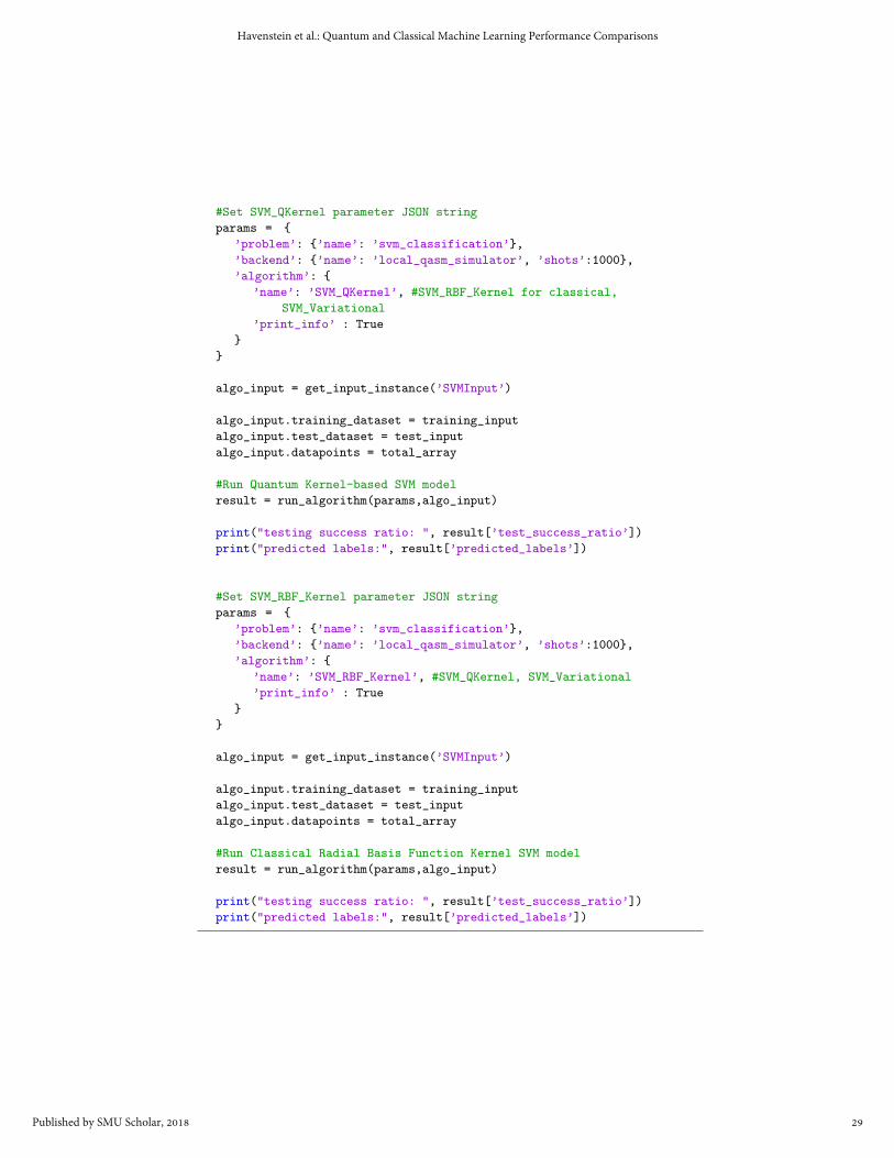
#Set SVM_QKernel parameter JSON string

params = {



’algorithm’: {

’name’: ’SVM_QKernel’, #SVM_RBF_Kernel for classical,

SVM_Variational


}

}





#Run Quantum Kernel-based SVM model




#Set SVM_RBF_Kernel parameter JSON string

params = {



’algorithm’: {

’name’: ’SVM_RBF_Kernel’, #SVM_QKernel, SVM_Variational


}

}





#Run Classical Radial Basis Function Kernel SVM model




29



Comparisons of Performance between Quantum and Classical ...

Documents

Transcript of Comparisons of Performance between Quantum and Classical ...