Classical and Quantum Ideal Gases

Chapter 2Classical and Quantum Ideal Gases

Abstract Bose and Einstein’s prediction of Bose–Einstein condensation came outof their theory for how quantum particles in a gas behaved, and was built on thepioneering statistical approach of Boltzmann for classical particles. Here we followBoltzmann, Bose and Einstein’s footsteps, leading to the derivation of Bose–Einsteincondensation for an ideal gas and its key properties.

2.1 Introduction

Consider the air in the room around you. We ascribe properties such as temperatureand pressure to characterise it, motivated by our human sensitivity to these prop-erties. However, the gas itself has a much finer level of detail, being composed ofspecks of dust, molecules and atoms, all in random motion. How can we explainthe macroscopic, coarse-grained appearance in terms of the fine-scale behaviour?An exact classical approach would proceed by solving Newton’s equation of motionfor each particle, based on the forces it experiences. For a typical room (volume∼50 m3, air particle density ∼2×1025 m−3 at room temperature and pressure) thiswould require solving around 1028 coupled ordinary differential equations, an utterlyintractable task. Since the macroscopic properties we experience are averaged overmany particles, a particle-by-particle description is unnecessarily complex. Instead itis possible to describe the fine-scale behaviour statistically through the methodologyof statistical mechanics. By specifying rules about how the particles behave and anyphysical constraints (boundaries, energy, etc.), the most likely macroscopic state ofthe system can be deduced.

Wedevelop these ideas for an ideal gas of N identical andnon-interactingparticles,with temperature T and confined to a box of volume V . The system is isolated, withno energy or particles entering or leaving the system1 Our aim is to predict theequilibrium state of the gas. After performing this for classical (point-like) particles,we extend it to quantum (blurry) particles. This leads directly to the prediction ofBose–Einstein condensation of an ideal gas. In doing so, we follow the seminal

1In the formalism of statistical mechanics, this is termed the microcanonical ensemble.

© The Author(s) 2016C.F. Barenghi and N.G. Parker, A Primer on Quantum Fluids,SpringerBriefs in Physics, DOI 10.1007/978-3-319-42476-7_2

9

10 2 Classical and Quantum Ideal Gases

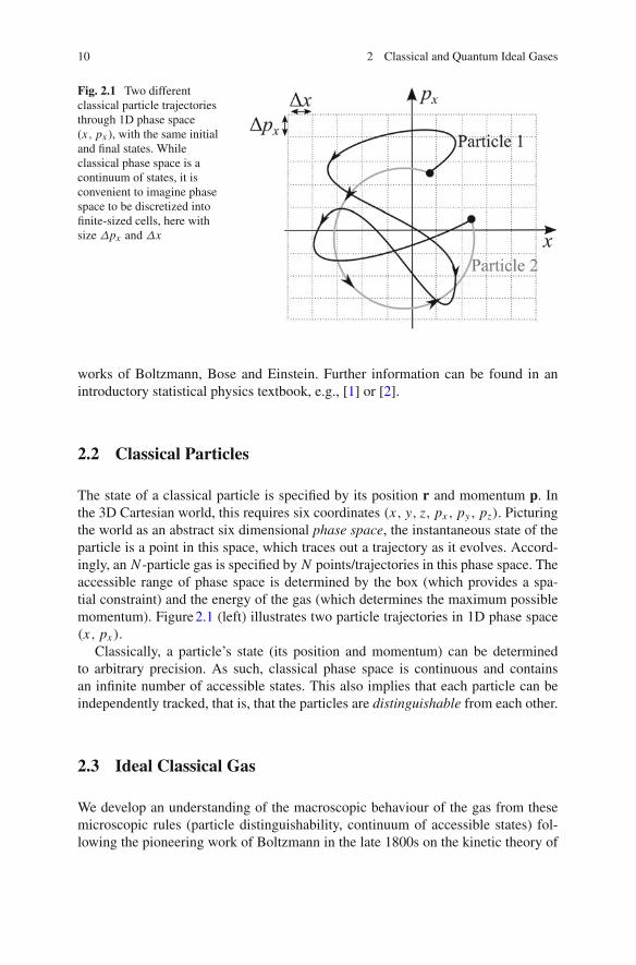
Fig. 2.1 Two differentclassical particle trajectoriesthrough 1D phase space(x, px ), with the same initialand final states. Whileclassical phase space is acontinuum of states, it isconvenient to imagine phasespace to be discretized intofinite-sized cells, here withsize Δpx and Δx

works of Boltzmann, Bose and Einstein. Further information can be found in anintroductory statistical physics textbook, e.g., [1] or [2].

2.2 Classical Particles

The state of a classical particle is specified by its position r and momentum p. Inthe 3D Cartesian world, this requires six coordinates (x, y, z, px , py, pz). Picturingthe world as an abstract six dimensional phase space, the instantaneous state of theparticle is a point in this space, which traces out a trajectory as it evolves. Accord-ingly, an N -particle gas is specified by N points/trajectories in this phase space. Theaccessible range of phase space is determined by the box (which provides a spa-tial constraint) and the energy of the gas (which determines the maximum possiblemomentum). Figure2.1 (left) illustrates two particle trajectories in 1D phase space(x, px ).

Classically, a particle’s state (its position and momentum) can be determinedto arbitrary precision. As such, classical phase space is continuous and containsan infinite number of accessible states. This also implies that each particle can beindependently tracked, that is, that the particles are distinguishable from each other.

2.3 Ideal Classical Gas

We develop an understanding of the macroscopic behaviour of the gas from thesemicroscopic rules (particle distinguishability, continuum of accessible states) fol-lowing the pioneering work of Boltzmann in the late 1800s on the kinetic theory of

2.3 Ideal Classical Gas 11

gases. Boltzmann’s work caused great controversy, as its particle and statistical basiswas at odds with the accepted view of matter as being continuous and determinis-tic. To overcome the practicalities of dealing with the infinity of accessible states,we imagine phase space to be discretized into cells of finite (but otherwise arbitrary)size, as shown in Fig. 2.1, and our N particles to be distributed across them randomly.Let there be M accessible cells, each characterised by its average momentum andposition. The number of particles in the i th cell—its occupancy number—is denotedas Ni . The number configuration across the whole system is specified by the fullset of occupancy numbers {N1, N2, . . . , NM }. We previously assumed that the totalparticle number is conserved, that is,

N =i=M∑

i=1

Ni .

Conservation of energy provides a further constraint; for now, however, we ignoreenergetic considerations.

2.3.1 Macrostates, Microstates and the Most LikelyState of the System

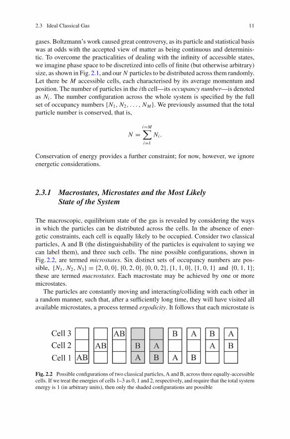
The macroscopic, equilibrium state of the gas is revealed by considering the waysin which the particles can be distributed across the cells. In the absence of ener-getic constraints, each cell is equally likely to be occupied. Consider two classicalparticles, A and B (the distinguishability of the particles is equivalent to saying wecan label them), and three such cells. The nine possible configurations, shown inFig. 2.2, are termed microstates. Six distinct sets of occupancy numbers are pos-sible, {N1, N2, N3} = {2, 0, 0}, {0, 2, 0}, {0, 0, 2}, {1, 1, 0}, {1, 0, 1} and {0, 1, 1};these are termed macrostates. Each macrostate may be achieved by one or moremicrostates.

The particles are constantly moving and interacting/colliding with each other ina random manner, such that, after a sufficiently long time, they will have visited allavailable microstates, a process termed ergodicity. It follows that each microstate is

Fig. 2.2 Possible configurations of two classical particles, A and B, across three equally-accessiblecells. If we treat the energies of cells 1–3 as 0, 1 and 2, respectively, and require that the total systemenergy is 1 (in arbitrary units), then only the shaded configurations are possible


equally likely (the assumption of “equal a priori probabilities”). Thus the most prob-ablemacrostate of the system is the onewith themostmicrostates. In our example, themacrostates {1, 1, 0}, {1, 0, 1} and {0, 1, 1} are most probable (having 2 microstateseach). In a physical gas, each macrostate corresponds to a particular macroscopicappearance, e.g. a certain temperature, pressure, etc. Hence, these abstract proba-bilistic notions become linked to the most likely macroscopic appearances of thegas.

For a more general macrostate {N1, N2, N3, .., NI }, the number of microstates is,

W = N !∏i Ni ! . (2.1)

Invoking the principle of equal a priori probabilities, the probability of being in thej th macrostate is,

Pr( j) = Wj∑j W j

. (2.2)

Wj , and hence Pr(j), is maximised for the most even distribution of particles acrossthe cells. This is true when each cell is equally accessible; as we discuss next, energyconsiderations modify the most preferred distribution across cells.

2.3.2 The Boltzmann Distribution

In the ideal-gas-in-a-box, each particle carries only kinetic energy p2/2m = (p2x +p2y + p2z )/2m. Having discretizing phase space, particle energy also becomes

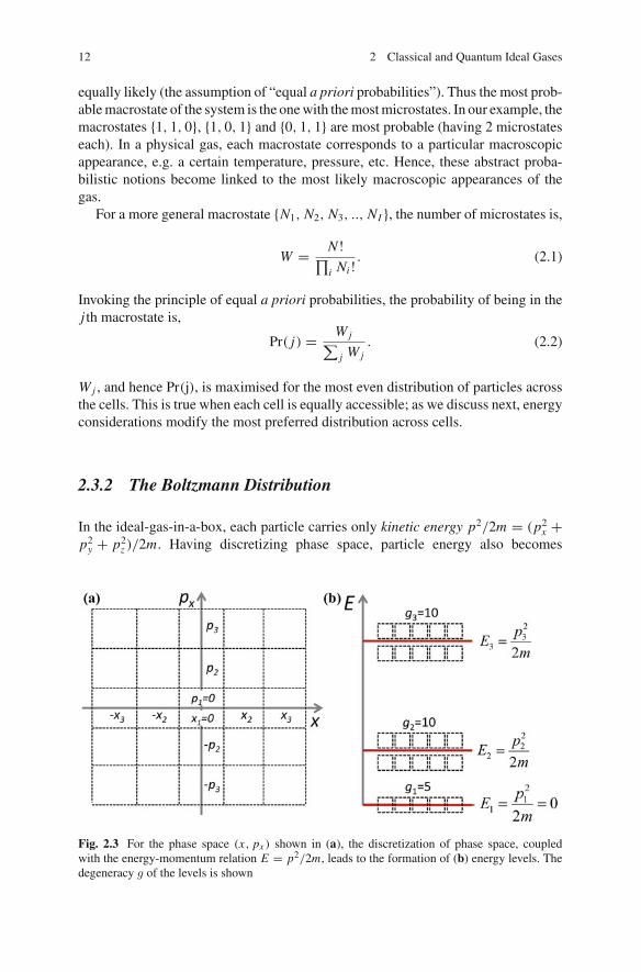
Fig. 2.3 For the phase space (x, px ) shown in (a), the discretization of phase space, coupledwith the energy-momentum relation E = p2/2m, leads to the formation of (b) energy levels. Thedegeneracy g of the levels is shown

2.3 Ideal Classical Gas 13

discretized, forming the notion of energy levels (familiar from quantum mechan-ics). This is illustrated in Fig. 2.3 for (x, px ) phase space. Three energy levels,E1 = 0, E2 = p21/2m and E3 = p22/2m, are formed from the five momentum values(p = 0,±p1,±p2). In two- and three-spatial dimensions, cells of energy Ei fall oncircles and spherical surfaces which satisfy p2x + p2y = 2mEi and p2x + p2y + p2z =2mEi , respectively. The lowest energy state E1 is the ground state; the higher energystates are excited states.

The total energy of the gas U is,

U =∑

i

Ni Ei ,

where Ei is the energy of cell i . TakingU to be conserved has important consequencesfor the microstates and macrostates. For example, imposing some arbitrary energyvalues in Fig. 2.2 restricts the allowed configurations. Particle occupation at highenergy is suppressed, skewing the distribution towards low energy.

For a system at thermal equilibrium with a large number of particles, onemacrostate (or a very narrow range of macrostates) will be greatly favoured. Thepreferred macrostate can be analytically predicted by maximising the number ofmicrostates W with respect to the set of occupancy numbers {N1, N2, N3, . . . , NI };details can be found in, e.g. [1, 2]. The result is,

Ni = fB(Ei ), (2.3)

where fB(E) is the famous Boltzmann distribution,

fB(E) = 1

e(E−μ)/kBT. (2.4)

The Boltzmann distribution tells us the most probable spread of particle occupancyacross states in an ideal gas, as a function of energy. This is associated with thethermodynamic equilibrium state. Here kB is Boltzmann’s constant (1.38 × 10−23 m2

kg s−2 K−1) and T is temperature (in Kelvin degrees, K). On average, each particlecarries kinetic energy 3

2kBT ( 12kBT in each direction of motion); this property isreferred to as the equipartition theorem.

The Boltzmann distribution function fB is normalized to the number of particles,N , as accommodated by the chemical potential μ. Writing A = eμ/kBT gives fB =A/eE/kBT , evidencing that A, and therebyμ, controls the amplitude of the distributionfunction.

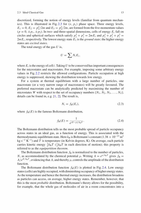
The Boltzmann distribution function fB(E) is plotted in Fig. 2.4. Low energystates (cells) are highly occupied,with diminishingoccupancyof higher energy states.As the temperature and hence the thermal energy increases, the distribution broadensas particles can access, on average, higher energy states. Remember, however, thatthis is the most probable distribution. Boltzmann’s theory allows for the possibility,for example, that the whole gas of molecules of air in a room concentrates into a


Fig. 2.4 The Boltzmanndistribution function fB(E)

for 3 different temperatures(the direction of increasingtemperature is indicated)

corner of the room. Due to the strong statistical bias towards an even distribution ofenergy, momenta and position, such an occurrence has incredibly low probability,but it is nonetheless possible, a fact which caused great discomfort with the scientificcommunity at the time.

It is often convenient towork in terms of the occupancy of energy levels rather thanstates (phase space cells). To relate the Boltzmann result to energy levels, we musttake into account the number of states in a given energy level, termed the degeneracyand denoted g j (we reserve i as the labelling of states). The occupation of the j thenergy level is then,

N j = g j fB(E j ). (2.5)

2.4 Quantum Particles

Having introduced classical particles, their statistics and the equilibrium propertiesof the ideal gas, nowwe turn to the quantum case. The statistics of quantum particles,developed in the 1920s, was pivotal to the development of quantum mechanics, pre-dating the well-known Schrödinger equation and uncertainty principle.

2.4.1 A Chance Discovery

Quantum physics arose from the failure of classical physics to describe the emissionof radiation from a black body in the ultraviolet range (the “ultraviolet catastrophe”).In 1900, Max Planck discovered a formula which empirically fit the data for allwavelengths and led him to propose that energy is emitted in discrete quanta of unitsh f (h being Planck’s constant and f the radiation frequency). Einstein extended thisidea with his 1905 prediction that the light itself was quantized.

The notion of quantum particles was discovered by accident. Around 1920, theIndian physicist Satyendra Bose was giving a lecture on the failure of the classical

2.4 Quantum Particles 15

theory of light using statistical arguments; a subtlemistake led to him prove the oppo-site. Indeed, he was able to derive Planck’s empirical formula from first principles,based on the assumptions that (a) the radiation particles are indistinguishable and(b) phase space was discretized into cells of size h3. Bose struggled at first to getthese results published and sought support from Nobel Laureate Einstein; Bose’spaper “Planck’s law and the light quantum hypothesis” was then published in 1924[3]. Soon after Einstein extended the idea to particles with mass in the paper “Quan-tum theory of the monoatomic ideal gas” [4].

The division of phase space was mysterious. Bose wrote “Concerning the kind ofsubdivision of this type, nothing definitive can be said”, while Einstein confided ina colleague that Bose’s “derivation is elegant but the essence remains obscure”. It isnow established as a fundamental property of particles, consistent with de Broglie’snotion of wave-particle duality (that particles are smeared out, over a lengthscalegiven by the de Broglie wavelength λdB = h/p) and with Heisenberg’s uncertaintyprinciple (that the position and momentum of a particle have an inherent uncertaintyΔxΔyΔzΔpxΔpyΔpz = h3). Each cell represents a distinct quantum state. Theindistinguishability of particles follows since it becomes impossible to distinguishtwo blurry particles in close proximity in phase space.

2.4.2 Bosons and Fermions

Quantum particles come in two varieties—bosons and fermions:

Fermions Soon after Bose and Einstein’s work, Fermi and Dirac developed Fermi-Dirac statistics for fermions. Fermions possess half-integer spin, and include elec-trons, protons and neutrons. Fermions obey the Pauli exclusion principle (Pauli,1925), which states that two identical fermions cannot occupy the same quantumstate simultaneously.

Bosons Bosons obey Bose–Einstein statistics, as developed by Bose and Einstein(above), and include photons and the Higgs boson. Bosons have integer spin, andsince spin is additive, composite bosons may be formed from equal numbers offermions, e.g. 4He, 87Rb and 23Na. Unlike fermions, any number of bosons canoccupy the same quantum state simultaneously.

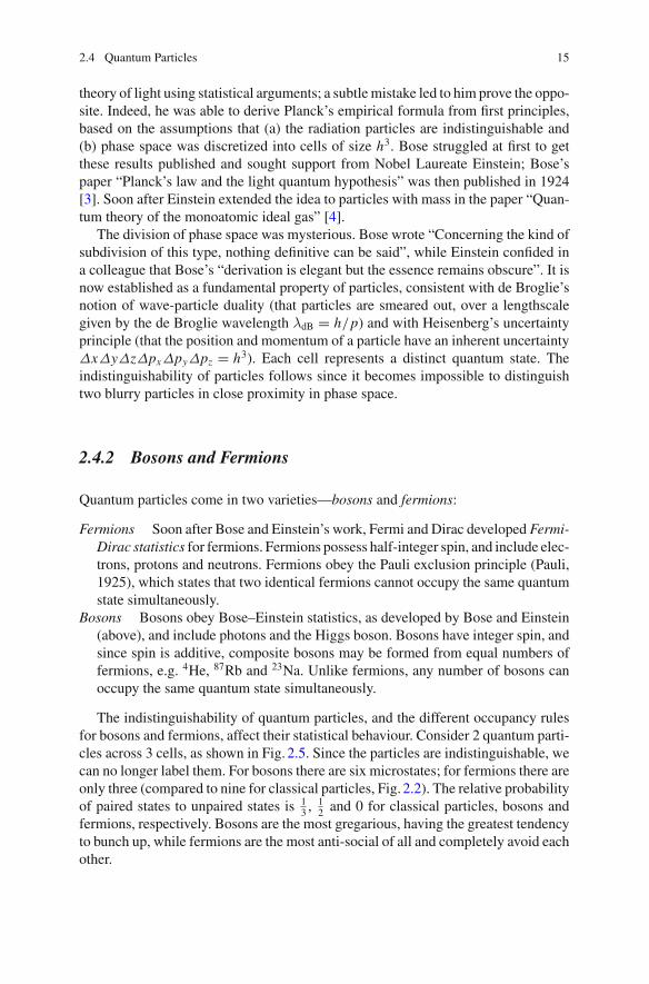
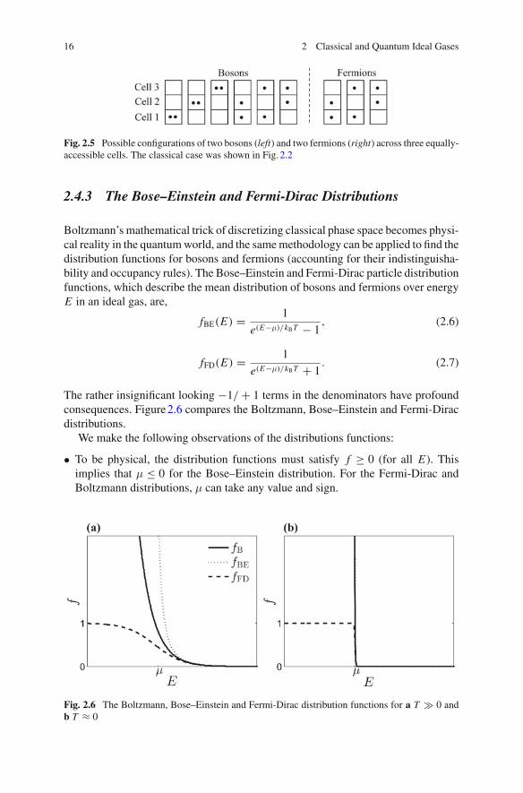
The indistinguishability of quantum particles, and the different occupancy rulesfor bosons and fermions, affect their statistical behaviour. Consider 2 quantum parti-cles across 3 cells, as shown in Fig. 2.5. Since the particles are indistinguishable, wecan no longer label them. For bosons there are six microstates; for fermions there areonly three (compared to nine for classical particles, Fig. 2.2). The relative probabilityof paired states to unpaired states is 1

3 ,12 and 0 for classical particles, bosons and

fermions, respectively. Bosons are the most gregarious, having the greatest tendencyto bunch up, while fermions are the most anti-social of all and completely avoid eachother.


Fig. 2.5 Possible configurations of two bosons (left) and two fermions (right) across three equally-accessible cells. The classical case was shown in Fig. 2.2

2.4.3 The Bose–Einstein and Fermi-Dirac Distributions

Boltzmann’s mathematical trick of discretizing classical phase space becomes physi-cal reality in the quantumworld, and the samemethodology can be applied to find thedistribution functions for bosons and fermions (accounting for their indistinguisha-bility and occupancy rules). The Bose–Einstein and Fermi-Dirac particle distributionfunctions, which describe the mean distribution of bosons and fermions over energyE in an ideal gas, are,

fBE(E) = 1

e(E−μ)/kBT − 1, (2.6)

fFD(E) = 1

e(E−μ)/kBT + 1. (2.7)

The rather insignificant looking −1/ + 1 terms in the denominators have profoundconsequences. Figure2.6 compares the Boltzmann, Bose–Einstein and Fermi-Diracdistributions.

We make the following observations of the distributions functions:

• To be physical, the distribution functions must satisfy f ≥ 0 (for all E). Thisimplies that μ ≤ 0 for the Bose–Einstein distribution. For the Fermi-Dirac andBoltzmann distributions, μ can take any value and sign.

Fig. 2.6 The Boltzmann, Bose–Einstein and Fermi-Dirac distribution functions for a T � 0 andb T ≈ 0

2.4 Quantum Particles 17

• For (E − μ)/kBT � 1, theBose–Einstein andFermi-Dirac distributions approachthe Boltzmann distribution. Here, the average state occupancy is much less thanunity, such that the effects of particle indistinguishability become negligible. Notethat the classical limit condition (E − μ)/kBT � 1 should not be interpreted toodirectly, as it seems to predict, counter-intuitively, that low temperatures favourclassical behaviour; this is because μ itself has a non-trivial temperature depen-dence.

• As E → μ from above, the Bose–Einstein distribution diverges, i.e. particles accu-mulate in the lowest energy states.

• For E � μ, the Fermi-Dirac distribution saturates to one particle per state, asrequired by the Pauli exclusion principle.

• For decreasing temperature, the distributions develop a sharper transition aboutE = μ, approaching step-like forms for T → 0.

2.5 The Ideal Bose Gas

Ayear after Einstein andBose set forth their newparticle statistics for a gas of bosons,Einstein published “Quantum theory of the monoatomic ideal gas: a second treatise”[5], elaborating on this topic. Here he predicted Bose–Einstein condensation. Wenow follow Einstein’s derivation of this phenomena and predict some key propertiesof the gas.

2.5.1 Continuum Approximation and Density of States

We consider an ideal (non-interacting) gas of bosons confined to a box, with energylevel occupation according to the Bose–Einstein distribution (2.6). For mathemat-ical convenience we approximate the discrete energy levels by a continuum, validproviding there are a large number of accessible energy levels. Replacing the levelvariables with continuous quantities (E j → E, g j → g(E) and N j → N (E)), thenumber of particles at energy E is written,

N (E) = fBE(E) g(E) = g(E)

e(E−μ)/kBT − 1, (2.8)

where g(E) is the density of states. The total number of particles and total energyfollow as the integrals,

N =∫

N (E) dE, (2.9)

U =∫

E N (E) dE . (2.10)


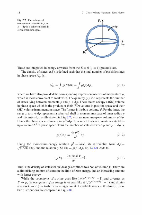
Fig. 2.7 The volume ofmomentum space from p top + dp is a spherical shell in3D momentum space

These are integrated in energy upwards from the E = 0 ( j = 1) ground state.The density of states g(E) is defined such that the total number of possible states

in phase space Nps is,

Nps =∫

g(E)dE =∫

g(p)dp, (2.11)

where we have also provided the corresponding expression in terms of momentum p,which is more convenient to work with. The quantity g(p)dp represents the numberof states lying between momenta p and p + dp. These states occupy a (6D) volumein phase space which is the product of their (3D) volume in position space and their(3D) volume inmomentum space. The former is the box volume,V . For the latter, therange p to p + dp represents a spherical shell in momentum space of inner radius pand thickness dp, as illustrated in Fig. 2.7, with momentum-space volume 4π p2dp.Hence the phase space volume is 4π p2Vdp. Now recall that each quantum state takesup a volume h3 in phase space. Thus the number of states between p and p + dp is,

g(p)dp = 4π p2Vh3

dp. (2.12)

Using the momentum-energy relation p2 = 2mE , its differential form dp =√m/2E dE), and the relation g(E) dE = g(p) dp, Eq. (2.12) leads to,

g(E) = 2π(2m)32V

h3E

12 . (2.13)

This is the density of states for an ideal gas confined to a box of volume V . There area diminishing amount of states in the limit of zero energy, and an increasing amountwith larger energy.

While the occupancy of a state goes like 1/(e(E−μ)/kBT − 1) and diverges asE → μ, the occupancy of an energy level goes like E

12 /(e(E−μ)/kBT − 1) and dimin-

ishes as E → 0 (due to the decreasing amount of available states in this limit). Thesetwo distributions are compared in Fig. 2.8a.

2.5 The Ideal Bose Gas 19

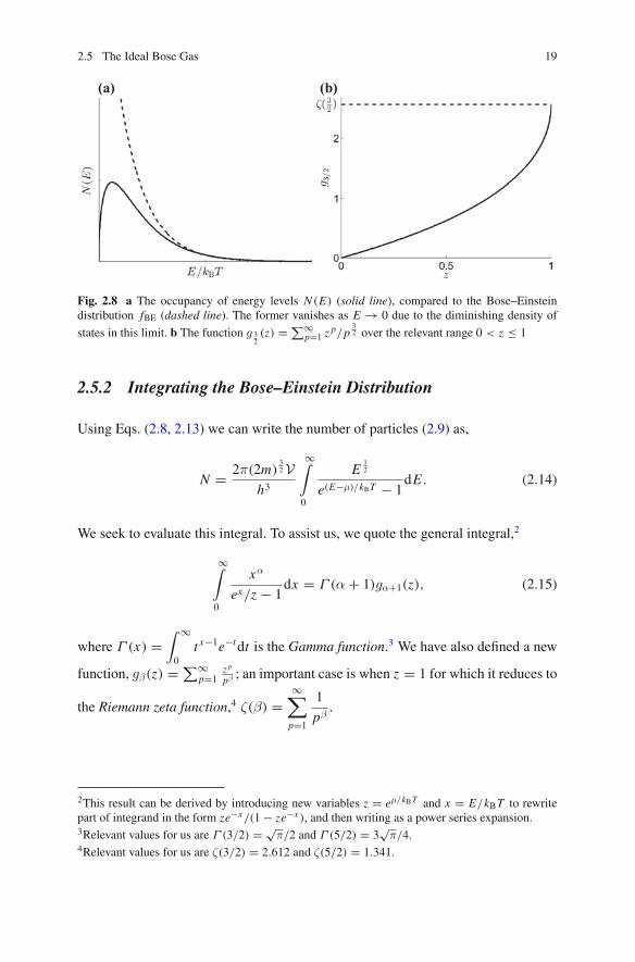
Fig. 2.8 a The occupancy of energy levels N (E) (solid line), compared to the Bose–Einsteindistribution fBE (dashed line). The former vanishes as E → 0 due to the diminishing density of

states in this limit. b The function g 32(z) = ∑∞

p=1 zp/p

32 over the relevant range 0 < z ≤ 1

2.5.2 Integrating the Bose–Einstein Distribution

Using Eqs. (2.8, 2.13) we can write the number of particles (2.9) as,

N = 2π(2m)32V

h3

∞∫

0

E12

e(E−μ)/kBT − 1dE . (2.14)

We seek to evaluate this integral. To assist us, we quote the general integral,2

∞∫

0

xα

ex/z − 1dx = Γ (α + 1)gα+1(z), (2.15)

where Γ (x) =∫ ∞

0t x−1e−tdt is the Gamma function.3 We have also defined a new

function, gβ(z) = ∑∞p=1

z p

pβ ; an important case is when z = 1 for which it reduces to

the Riemann zeta function,4 ζ(β) =∞∑

p=1

1

pβ.

2This result can be derived by introducing new variables z = eμ/kBT and x = E/kBT to rewritepart of integrand in the form ze−x/(1 − ze−x ), and then writing as a power series expansion.3Relevant values for us are Γ (3/2) = √

π/2 and Γ (5/2) = 3√

π/4.4Relevant values for us are ζ(3/2) = 2.612 and ζ(5/2) = 1.341.


Taking α = 12 , x = E/kBT and z = eμ/kBT in the general result (2.15), we eval-

uate Eq. (2.14) as,

N = (2πmkBT )32V

h3g 3

2(z), (2.16)

where we have used the result Γ (3/2) = √π/2. Note that the relevant range of z

is 0 < z ≤ 1: the lower limit is required since z = eμ/kBT > 0 while the upper limitz ≤ 1 is required to prevent negative populations. Note also that μ ≤ 0 over thisrange, as required for the Bose–Einstein distribution (recall Sect. 2.4.3). In Fig. 2.8bwe plot g 3

2(z) over this range.

2.5.3 Bose–Einstein Condensation

The prediction of Bose–Einstein condensation in the style of Einstein arises directlyfrom Eq. (2.16). Consider adding particles to the box, while at constant temperature.An increase in N is accommodated by an increase in the function g 3

2(z). However,

g 32(z) is finite, reaching a maximum value of g 3

2= ζ( 32 ) = 2.612 at z = 1. In other

words, the system becomes saturatedwith particles. This critical number of particles,denoted Nc, follows as,

Nc = (2πmkBT )32V

h3ζ(

3

2). (2.17)

Our derivation predicts a limit to how many particles the Bose–Einstein distribu-tion can hold, but common sense tells us that it should always be possible to addmoreparticles to the box. In fact, we made a subtle mistake. In calculating N we replacedthe summation over discrete energy levels (from the i = 1 ground state upwards) byan integral over a continuum of energies (from E = 0 upwards). However, this con-tinuum approximation does not properly account for the population of the groundstate, since the density of states, g(E) ∝ E

12 , incorrectly predicts zero population

in the ground state. What we have predicted is the saturation of the excited states;any additional particles added to the system enter the ground state (which comesat no energetic cost). For N � Nc, the ground state acquires an anomalously largepopulation.

As Einstein put it [5], “a number of atoms which always grows with total densitymakes a transition to the ground quantum state, whereas the remaining atoms distrib-ute themselves... A separation occurs; a part condenses, the rest remains a saturatedideal gas.” This effect is Bose–Einstein condensation, and the collection of particlesin the ground state is the Bose–Einstein condensate. The effect is a condensation inmomentum space, referring to the occupation of the zero momentum state. In prac-tice, when the system is confined by a potential, a condensation in real space alsotakes place, towards the region of lowest potential. Bose–Einstein condensation isa phase transition, but whereas conventional phase transitions (e.g. transformation


from gas to liquid or liquid to solid) are driven by particle interactions, Bose–Einsteincondensation is driven by the particle statistics.

Based on the above hindsight, we note that the total atom number N appearing inEqs. (2.9), (2.14) and (2.16) should be replaced by the number in excited states, Nex.

2.5.4 Critical Temperature for Condensation

If, instead, the particle number and volume are fixed, then there exists a critical tem-perature Tc below which condensation occurs. The population of excited particles ata given temperature is given by Eq. (2.16). For T > Tc, this is sufficient to accommo-date all of the particles, and the gas is in the normal phase. As temperature is lowered,however, the excited state capacity also decreases. At the point where the excitedstates no longer accommodate all the particles, Bose–Einstein condensation occurs.The critical temperature is obtained by setting z = 1 in Eq. (2.16) and rearrangingfor T ,

Tc = h2

2πmkB

(N

ζ( 32 )V

) 23

. (2.18)

For further decreases in temperature, Nex decreases and so more and more particlesmust enter the ground state. In the limit T → 0, excited states can carry no particlesand all particles enter the condensate.

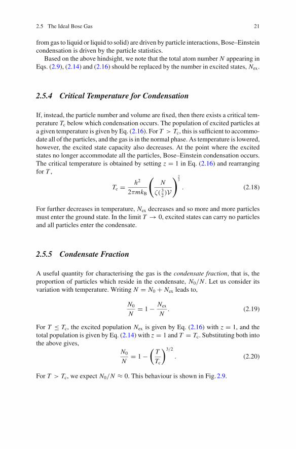
2.5.5 Condensate Fraction

A useful quantity for characterising the gas is the condensate fraction, that is, theproportion of particles which reside in the condensate, N0/N . Let us consider itsvariation with temperature. Writing N = N0 + Nex leads to,

N0

N= 1 − Nex

N. (2.19)

For T ≤ Tc, the excited population Nex is given by Eq. (2.16) with z = 1, and thetotal population is given by Eq. (2.14) with z = 1 and T = Tc. Substituting both intothe above gives,

N0

N= 1 −

(T

Tc

)3/2

. (2.20)

For T > Tc, we expect N0/N ≈ 0. This behaviour is shown in Fig. 2.9.


Fig. 2.9 a Illustration ofenergy level occupations inthe boxed ideal Bose gas. AtT = 0 all particles lie in theground state. For0 < T < Tc, some particlesare in excited levels but thereis still macroscopicoccupation of the groundstate. For T > Tc, there isnegligible occupation of theground state. b Variation ofcondensate fraction, N0/N ,with temperature, as perEq. (2.20)

2.5.6 Particle-Wave Overlap

Bose–Einstein condensation occurs when N > Nc, with Nc given by Eq. (2.17).It is equivalent to write this criterion in terms of the number density of particles,n = N/V , as,

n > ζ

(3

2

)(2πmkBT )3/2

h3. (2.21)

According to de Broglie, particles behave like waves, with a wavelength λdB = h/p.

For a thermally-excited gas, the particle wavelength is λdB = h√2πmkBT

. Employ-

ing this, the above criterion becomes,

nλ3dB > ζ

(3

2

). (2.22)

Upon noting that the average inter-particle distance d = n− 13 and ζ( 32 )

13 ∼ 1 we

arrive at,

λdB � d. (2.23)

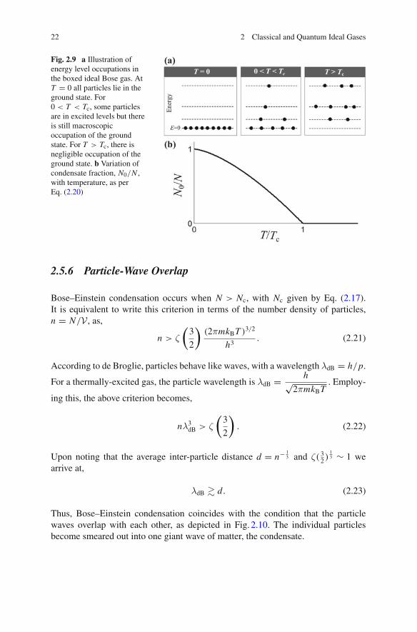
Thus, Bose–Einstein condensation coincides with the condition that the particlewaves overlap with each other, as depicted in Fig. 2.10. The individual particlesbecome smeared out into one giant wave of matter, the condensate.


Fig. 2.10 Schematic of the transition between a classical gas and a Bose–Einstein condensate. Athigh temperatures (T � Tc) the gas is a thermal gas of point-like particles. At low temperatures(but still exceeding Tc) the de Broglie wavelength λdB becomes significant, yet smaller than theaverage spacing d. At Tc, the matter waves overlap (λdB ∼ d), marking the onset of Bose–Einsteincondensation

2.5.7 Internal Energy

The internal energy of the gas U is determined by the excited states only, since theground state possesses zero energy; therefore we can expressU by integrating acrossthe excited state particles as,

U =∞∫

0

E Nex(E) dE . (2.24)

Upon evaluating this integral below and above Tc we find,

U =

⎧⎪⎪⎨

⎪⎪⎩

3

2

ζ(5/2)

ζ(3/2)NkBT

(T

Tc

)3/2

for T < Tc,

3

2NkBT for T � Tc.

(2.25)

The T � Tc result is consistent with the classical equipartition theorem for an idealgas, which states that each particle has on average 1

2kBT of kinetic energy per direc-tion of motion. The different behavior for T < Tc confirms the presence of a distinctstate of matter.


2.5.8 Pressure

The pressure of an ideal gas is P = 2U/3V . From Eq. (2.25), then for T � Tc werecover the standard result for a classical ideal gas that P ∝ T/V . For T < Tc, andrecalling that Tc ∝ 1/V2/3, we find that P ∝ T 5/2. The pressure of the condensate iszero at absolute zero and does not depend on the volume of the box! A consequenceof this is that the condensate has infinite compressibility, as explored in Problem 2.6.

2.5.9 Heat Capacity

The heat capacity of a substance is the energy required to raise its temperature byunit amount. At constant volume it is defined as,

CV =(

∂U

∂T

)

V. (2.26)

From Eq. (2.25) we find,

CV =⎧⎨

⎩1.93NkBT 3/2 for T < Tc,3

2NkB for T � Tc.

(2.27)

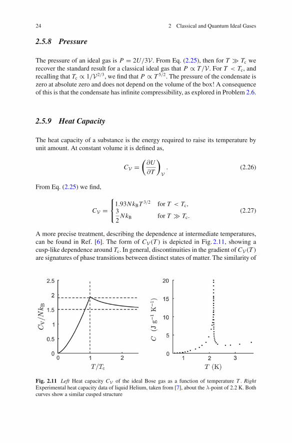
A more precise treatment, describing the dependence at intermediate temperatures,can be found in Ref. [6]. The form of CV(T ) is depicted in Fig. 2.11, showing acusp-like dependence around Tc. In general, discontinuities in the gradient of CV(T )

are signatures of phase transitions between distinct states of matter. The similarity of

Fig. 2.11 Left Heat capacity CV of the ideal Bose gas as a function of temperature T . RightExperimental heat capacity data of liquid Helium, taken from [7], about the λ-point of 2.2 K. Bothcurves show a similar cusped structure


this prediction to measured heat capacity curves for Helium about the λ-point waskey evidence in linking helium II to Bose–Einstein condensation.

2.5.10 Ideal Bose Gas in a Harmonic Trap

2.5.10.1 Critical Temperature and Condensate Fraction

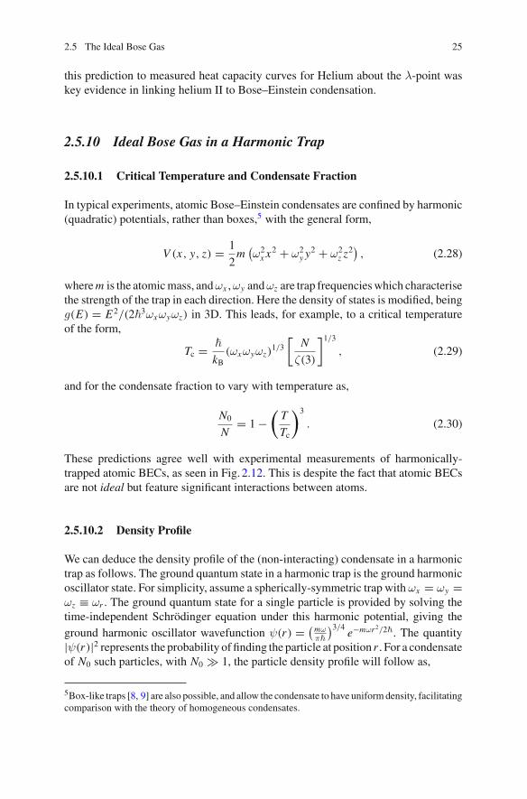
In typical experiments, atomic Bose–Einstein condensates are confined by harmonic(quadratic) potentials, rather than boxes,5 with the general form,

V (x, y, z) = 1

2m

(ω2x x

2 + ω2y y

2 + ω2z z

2), (2.28)

wherem is the atomicmass, andωx ,ωy andωz are trap frequencieswhich characterisethe strength of the trap in each direction. Here the density of states is modified, beingg(E) = E2/(2�

3ωxωyωz) in 3D. This leads, for example, to a critical temperatureof the form,

Tc = �

kB(ωxωyωz)

1/3

[N

ζ(3)

]1/3

, (2.29)

and for the condensate fraction to vary with temperature as,

N0

N= 1 −

(T

Tc

)3

. (2.30)

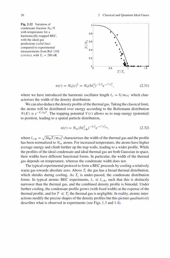
These predictions agree well with experimental measurements of harmonically-trapped atomic BECs, as seen in Fig. 2.12. This is despite the fact that atomic BECsare not ideal but feature significant interactions between atoms.

2.5.10.2 Density Profile

We can deduce the density profile of the (non-interacting) condensate in a harmonictrap as follows. The ground quantum state in a harmonic trap is the ground harmonicoscillator state. For simplicity, assume a spherically-symmetric trap with ωx = ωy =ωz ≡ ωr . The ground quantum state for a single particle is provided by solving thetime-independent Schrödinger equation under this harmonic potential, giving theground harmonic oscillator wavefunction ψ(r) = (

mωπ�

)3/4e−mωr2/2�. The quantity

|ψ(r)|2 represents the probability of finding the particle at position r . For a condensateof N0 such particles, with N0 � 1, the particle density profile will follow as,

5Box-like traps [8, 9] are also possible, and allow the condensate to have uniformdensity, facilitatingcomparison with the theory of homogeneous condensates.


Fig. 2.12 Variation ofcondensate fraction N0/Nwith temperature for aharmonically-trapped BEC,with the ideal-gaspredictions (solid line)compared to experimentalmeasurements from Ref. [10](circles), with Tc = 280 nK

n(r) = N0|ψ|2 = N0(��2r )−3/2e−r2/�2r , (2.31)

where we have introduced the harmonic oscillator length �r = �/mωr which char-acterises the width of the density distribution.

Wecan also deduce the density profile of the thermal gas. Taking the classical limit,the atoms will be distributed over energy according to the Boltzmann distributionN (E) ∝ e−E/kBT . The trapping potential V (r) allows us to map energy (potential)to position, leading to a spatial particle distribution,

n(r) = Nex(��2r,th)−3/2e−r2/�2r,th , (2.32)

where �r,th = √2kBT/mω2

r characterises the width of the thermal gas and the profilehas been normalized to Nex atoms. For increased temperature, the atoms have higheraverage energy and climb further up the trap walls, leading to a wider profile. Whilethe profiles of the ideal condensate and ideal thermal gas are both Gaussian in space,their widths have different functional forms. In particular, the width of the thermalgas depends on temperature, whereas the condensate width does not.

The typical experimental protocol to form a BEC proceeds by cooling a relativelywarm gas towards absolute zero. Above Tc the gas has a broad thermal distribution,which shrinks during cooling. As Tc is under-passed, the condensate distributionforms. In typical atomic BEC experiments, �r � �r,th, such that this is distinctlynarrower than the thermal gas, and the combined density profile is bimodal. Underfurther cooling, the condensate profile grows (with fixed width) at the expense of thethermal profile, and for T � Tc the thermal gas is negligible. In reality, atomic inter-actions modify the precise shapes of the density profiles but this picture qualitativelydescribes what is observed in experiments (see Figs. 1.3 and 1.4).

http://dx.doi.org/10.1007/978-3-319-42476-7_1

http://dx.doi.org/10.1007/978-3-319-42476-7_1

2.6 Ideal Fermi Gas 27

2.6 Ideal Fermi Gas

We outline the corresponding behaviour of the ideal Fermi gas. Since (identical)fermions are restricted to up to one per state, Bose–Einstein condensation is prohib-ited, and the Fermi gas behaves very differently as T → 0. At T = 0 the Fermi-Diracdistribution (2.7) reduces to a step function,

fFD(E) ={1 forE ≤ EF,

0 forE > EF.(2.33)

All states are occupied up to an energy threshold EF, termed the Fermi energy (equalto the T = 0 chemical potential).With this simplified distribution it is straightforwardto integrate the number of particles,

N =∫

N (E) dE =EF∫

0

g(E) fFD(E) dE = 4πV3

(2mEF

h2

)3/2

, (2.34)

where we have used the density of states (2.13). Note that the continuum approxi-mation N = ∫

g(E) N (E) dE holds for N � 1 fermions since the unit occupationof the ground state is always negligible. Rearranging for the Fermi energy in termsof the particle density n = N/V gives,

EF = �2

2m

(6π2n

)2/3. (2.35)

From this we define the Fermi momentum pF = �kF where kF = (6π2n)1/3 is theFermi wavenumber. In momentum space, all states are occupied up to momentumpF, termed the Fermi sphere.

Similarly, the total energy of the gas at T = 0 is,

U =∫

N (E)E dE = 4πV5

(2m

h2

)3/2

E5/2F = 3

5NEF. (2.36)

From the pressure relation for an ideal gas, P = 2U/3V , the pressure of the idealFermi gas at T = 0 is,

P = 2

5nEF. (2.37)

This pressure is finite even at T = 0, unlike the Bose and classical gases, and doesnot arise from thermal agitation. Instead it is due to the stacking up of particles inenergy levels, as constrained by the quantum rules for fermions. This degeneracypressure prevents very dense stars, such as neutron stars, from collapsing under theirown gravitational fields.


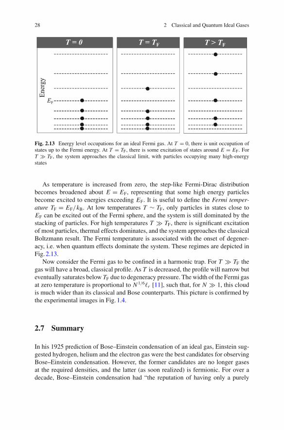
Fig. 2.13 Energy level occupations for an ideal Fermi gas. At T = 0, there is unit occupation ofstates up to the Fermi energy. At T = TF, there is some excitation of states around E = EF. ForT � TF, the system approaches the classical limit, with particles occupying many high-energystates

As temperature is increased from zero, the step-like Fermi-Dirac distributionbecomes broadened about E = EF, representing that some high energy particlesbecome excited to energies exceeding EF. It is useful to define the Fermi temper-ature TF = EF/kB. At low temperatures T ∼ TF, only particles in states close toEF can be excited out of the Fermi sphere, and the system is still dominated by thestacking of particles. For high temperatures T � TF, there is significant excitationof most particles, thermal effects dominates, and the system approaches the classicalBoltzmann result. The Fermi temperature is associated with the onset of degener-acy, i.e. when quantum effects dominate the system. These regimes are depicted inFig. 2.13.

Now consider the Fermi gas to be confined in a harmonic trap. For T � TF thegas will have a broad, classical profile. As T is decreased, the profile will narrow buteventually saturates below TF due to degeneracy pressure. The width of the Fermi gasat zero temperature is proportional to N 1/6�r [11], such that, for N � 1, this cloudis much wider than its classical and Bose counterparts. This picture is confirmed bythe experimental images in Fig. 1.4.

2.7 Summary

In his 1925 prediction of Bose–Einstein condensation of an ideal gas, Einstein sug-gested hydrogen, helium and the electron gas were the best candidates for observingBose–Einstein condensation. However, the former candidates are no longer gasesat the required densities, and the latter (as soon realized) is fermionic. For over adecade, Bose–Einstein condensation had “the reputation of having only a purely

http://dx.doi.org/10.1007/978-3-319-42476-7_1

2.7 Summary 29

imaginary character” [12], deemed too fragile to occur in real gases with their finitesize and particle interactions. In 1938 Einstein’s idea became revived when FritzLondon recognized the similarity to the heat capacity curves in Helium as it enteredthe superfluid phase. It took several more decades to cement this link with micro-scopic theory. Bose–Einstein condensation is now know to underly superfluid He4

and He3, superconductors and the ultracold atomic Bose gases. We explore the latterin the next chapter.

Problems

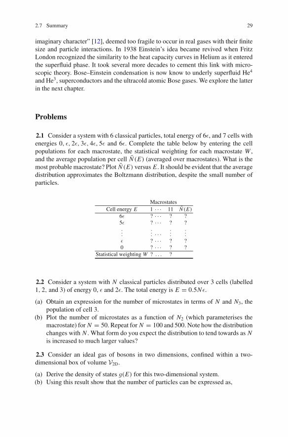
2.1 Consider a system with 6 classical particles, total energy of 6ε, and 7 cells withenergies 0, ε, 2ε, 3ε, 4ε, 5ε and 6ε. Complete the table below by entering the cellpopulations for each macrostate, the statistical weighting for each macrostate W ,and the average population per cell N̄ (E) (averaged over macrostates). What is themost probable macrostate? Plot N̄ (E) versus E . It should be evident that the averagedistribution approximates the Boltzmann distribution, despite the small number ofparticles.

MacrostatesCell energy E 1 · · · 11 N̄ (E)

6ε ? · · · ? ?5ε ? · · · ? ?...

.

.

. · · ·...

.

.

.

ε ? · · · ? ?0 ? · · · ? ?

Statistical weighting W ? . . . ?

2.2 Consider a system with N classical particles distributed over 3 cells (labelled1, 2, and 3) of energy 0, ε and 2ε. The total energy is E = 0.5Nε.

(a) Obtain an expression for the number of microstates in terms of N and N3, thepopulation of cell 3.

(b) Plot the number of microstates as a function of N2 (which parameterises themacrostate) for N = 50. Repeat for N = 100 and 500. Note how the distributionchanges with N . What form do you expect the distribution to tend towards as Nis increased to much larger values?

2.3 Consider an ideal gas of bosons in two dimensions, confined within a two-dimensional box of volume V2D.

(a) Derive the density of states g(E) for this two-dimensional system.(b) Using this result show that the number of particles can be expressed as,


Nex = 2πmV2DkBT

h2

∫ ∞

0

ze−x

1 − ze−xdx,

where z = eμ/kBT and x = E/kBT . Solve this integral using the substitutiony = ze−x .

(c) Obtain an expression for the chemical potential μ and thereby show that Bose–Einstein condensation is possible only at T = 0.

2.4 Equation (2.25) summarizes how the internal energy of the boxed 3D ideal Bosegas scales with temperature. Derive the full expressions for the internal energy forthe two regimes (a) T < Tc (for which z = 1), and (b) T � Tc (for which z � 1).Extend your results to derive the expressions for the heat capacity given in Eq. (2.27).

2.5 Bose–Einstein condensates are typically confined in harmonic trapping poten-tials, as given by Eq. (2.28). Using the corresponding density of states provided inSect. 2.5.10.1:

(a) Derive the expression for the critical number of particles.(b) Derive the expression (2.29) for the critical temperature.(c) Determine the expression (2.30) for the variation of condensate fraction N0/N

with T/Tc.(d) In one of the first BEC experiments, a gas of 40, 000 Rubidium-87 atoms (atomic

mass 1.45 × 10−25 kg) underwent Bose–Einstein condensation at a temperatureof 280 nK. The harmonic trap was spherically-symmetric with with ωr = 1130Hz. Calculate the critical temperature according to the ideal Bose gas prediction.Howdoes this compare to the result for the boxedgas (youmayassume the atomicdensity as 2.5 × 1018 m−3).

2.6 The compressibility β of a gas, a measure of how much it shrinks in responseto a compressional force, is defined as,

β = − 1

V∂V∂P

.

Determine the compressibility of the ideal gas for T < Tc.Hint: Since Tc is a function of V , you should ensure the full V-dependence is

present before differentiating.

References

1. F. Mandl, Statistical Physics, 2nd edn. (Wiley, Chichester, 1988)2. L.D. Landau, E.M. Lifshitz, Statistical Physics, 3rd edn. (Elsevier, Oxford, 1980)3. S.N. Bose, Z. Phys. 26, 178 (1924)4. A. Einstein, Kgl. Preuss. Akad. Wiss. 261 (1924)5. A. Einstein, Kgl. Preuss. Akad. Wiss. 3 (1925)

References 31

6. L.P. Pitaevskii, S. Stringari, Bose-Einstein Condensation (International Series of Monographson Physics) (Oxford Science Publications, Oxford, 2003)

7. M.J. Buckingham, W.M. Fairbank, The nature of the lambda-transition in liquid helium, inProgress in Low Temperature Physics, vol. 3, ed. by C.J. Gorter (North Holland, Amsterdam,1961)

8. A.L. Gaunt, T.F. Schmidutz, I. Gotlibovych, R.P. Smith, Z. Hadzibabic, Phys. Rev. Lett. 110,200406 (2013)

9. L. Chomaz et al., Nat. Comm. 6, 6162 (2015)10. J.R. Ensher, D.S. Jin, M.R. Matthews, C.E. Wieman, E.A. Cornell, Phys. Rev. Lett. 77, 4984

(1996)11. D.A. Butts, D.S. Rokhsar, Phys. Rev. A 55, 4346 (1997)12. F. London, Nature 141, 643 (1938)

http://www.springer.com/978-3-319-42474-3

Classical and Quantum Ideal Gases

Documents

Transcript of Classical and Quantum Ideal Gases