Comparison of Five Modeling Approaches to Quantify and ...

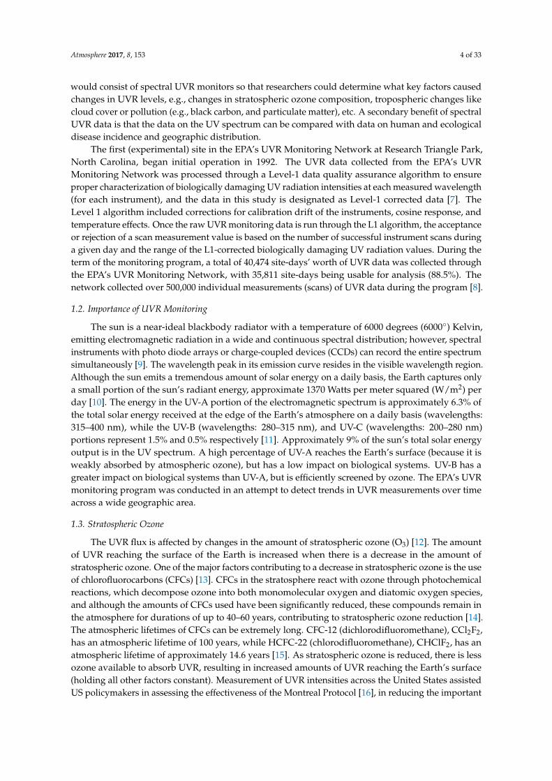
atmosphere

Article

Comparison of Five Modeling Approaches toQuantify and Estimate the Effect of Clouds on theRadiation Amplification Factor (RAF) for SolarUltraviolet Radiation

Eric S. Hall ID

National Exposure Research Laboratory, Office of Research and Development, US Environmental ProtectionAgency, Mail Drop E205-03, 109 T. W. Alexander Drive, Research Triangle Park, NC 27711, USA;[email protected]

Received: 16 June 2017; Accepted: 16 August 2017; Published: 18 August 2017

Abstract: A generally accepted value for the Radiation Amplification Factor (RAF), with respect tothe erythemal action spectrum for sunburn of human skin, is −1.1, indicating that a 1.0% increasein stratospheric ozone leads to a 1.1% decrease in the biologically damaging UV radiation in theerythemal action spectrum reaching the Earth. The RAF is used to quantify the non-linear changein the biologically damaging UV radiation in the erythemal action spectrum as a function of totalcolumn ozone (O3). Spectrophotometer measurements recorded at ten US monitoring sites wereused in this analysis, and over 71,000 total UVR measurement scans of the sky were collected atthose 10 sites between 1998 and 2000 to assess the RAF value. This UVR dataset was examined todetermine the specific impact of clouds on the RAF. Five de novo modeling approaches were used onthe dataset, and the calculated RAF values ranged from a low of −0.80 to a high of −1.38.

Keywords: Radiation Amplification Factor (RAF); solar zenith angle (SZA); Dobson Unit (DU);ultraviolet (UV); ultraviolet radiation (UVR); cloudiness

1. Introduction

The Radiation Amplification Factor (RAF) is defined as the measured percentage change inultraviolet (UV) irradiance for each one-percent change in total column ozone [1]. Understandingvariations in measured ultraviolet radiation (UVR) over time, along with associated RAF values,assists health scientists in determining risks associated with UVR exposure through the RAF forindividuals and the environment [2]. Exposure to ultraviolet radiation (UVR) poses risks to bothhumans and the environment, therefore a number of national and international government, industrial,and university research organizations initiated programs to measure the amount of UVR reachingthe Earth’s surface, since stratospheric ozone affects the amount of UVR reaching the Earth. TheUnited States Environmental Protection Agency (US EPA) conducted a research program from 1996to 2004 to measure ultraviolet radiation (UVR) at 21 network sites throughout the continental US,Alaska, Hawaii and the US Virgin Islands (St. John) under all weather conditions. The US EPANational Exposure Research Laboratory (NERL) developed the UV Radiation Research Program tomeasure intensity of UVR at distinct locations throughout the US that differed in spatial location,geography, climate, altitude, and ecology. The three major categories of research-grade instrumentsthat have been used to detect UVR are broadband, narrowband, and spectral. NERL chose spectralUVR monitors called Brewer Spectrophotometers. When operated within a disciplined calibration andmaintenance program, the instruments precisely measure UVR levels through a well-defined portionof electromagnetic spectrum wavelengths (286.5 nm to 363 nm). Maintaining long-term calibration

Atmosphere 2017, 8, 153; doi:10.3390/atmos8080153 www.mdpi.com/journal/atmosphere

http://www.mdpi.com/journal/atmosphere

http://www.mdpi.com

https://orcid.org/0000-0002-0528-2014

http://dx.doi.org/10.3390/atmos8080153

http://www.mdpi.com/journal/atmosphere

Atmosphere 2017, 8, 153 2 of 33

of spectral instruments requires great effort. They are more expensive to operate in comparison tobroadband or narrowband instruments, because they require highly skilled operators.

The Brewer instruments were calibrated for biologically damaging UV radiation in the erythemalaction spectrum at each of the 21 sites using a secondary (travelling) standard lamp traceable toa primary (stationary) National Institute of Standards and Technology (NIST) 1000-W lamp. Thecalibrations were performed by scientists at the University of Georgia at Athens (UGA) National UVMonitoring Center (NUVMC) on an annual basis. The calibrated Brewer data used a daily temporalresponse (estimated) based on the annual calibration. In addition, independent quality assuranceaudits of the Brewers were performed by scientists from the National Oceanic and AtmosphericAdministration (NOAA) Central UV Calibration Facility (CUCF). Quarterly checks on the transferof the calibration standard from the NIST 1000-W lamp to the traveling secondary standard wereperformed at the NUVMC. The response function of each instrument was calculated daily from a linearinterpolation between the two (temporally) closest response functions. Brewer data were corrected fordark count, dead time, and stray light.

Clouds affect the relative absorption/reflectance of UVR. Transmittance of UVR through cloudsis shown to be wavelength dependent, ranging from 45% in the UV-A region to 60% in the UV-Bregion as stated in Chapter 4, page 105 of [3]. Cloud features known to affect the transmission of UVRinclude cloud amount and coverage (e.g., percentage of sky covered), particle size distribution, cloudspatial and temporal variability, season, location, etc., [4]. Realistically, clouds can either increase ordecrease the amount of UVR at the surface [5]. Due to the unpredictable nature of clouds, the extentof cloudiness (percent clearness) of the sky had to be determined for this analysis in a consistent,logically defensible manner, to determine the effect of clouds on the Radiation Amplification Factor(RAF). Using a consistent definition of cloudiness, the results seem to indicate that average RAF valuesgenerally approximate −1.1 at these 10 sites (two urban sites and eight US National Parks sites),and that total column ozone (O3) and solar zenith angle (SZA) are the most important parametersin determining the biologically damaging UV radiation in the erythemal action spectrum reachingthe Earth’s surface. Five modeling approaches, labelled A, B, C, D, and E, were used to estimate theimpact of clouds on the biologically damaging UV radiation in the erythemal action spectrum.

1.1. Development of the EPA’s UVR Monitoring Network

In the early 1990s, the EPA’s Office of Research and Development (ORD) originally designed aUVR monitoring network of five to seven sites principally in urban areas, with a few “pristine” ruralsites for monitoring background UVR levels. The EPA’s role in UVR research was to monitor in urbanareas. The United States Department of Agriculture (USDA) was responsible for monitoring UVR inrural areas. The focus of the EPA’s original UVR network design was shifted in 1996. In September 1996,the US EPA and US National Parks Service (NPS), of the US Department of the Interior (DOI), signedan Interagency Agreement (IAG) to cooperate on a program of long-term monitoring of environmentalstressors, including UVR, at 21 separate locations throughout the United States. When the NPS siteswere added to the network, it greatly expanded the EPA’s UVR monitoring program. The EPA’sUVR Monitoring Network facilitated research on the observed effects that environmental stressors,including UVR, pose on various ecosystems and on human health. The 21 EPA UVR monitoring sites(displayed in Figure 1) were located throughout the continental United States, Alaska (Denali NationalPark), Hawaii (Hawaii Volcanoes National Park) and the US Virgin Islands (Virgin Islands NationalPark, St. Johns, VI). Fourteen of the sites were located in US National Parks, and seven sites werelocated in urban settings. Data collected from the 21 sites was processed through a quality assuranceprotocol to ensure proper characterization of UVR intensities measured at each site.

Atmosphere 2017, 8, 153 3 of 33

Atmosphere 2017, 8, 153 3 of 32

and dose rate of UVR received at the Earth’s surface at various times throughout the day. The instruments were mounted on an azimuth tracker and tripod unit connected to a desktop computer running the Disk Operating System (DOS) and GWTM Basic Software for instrument control.

The major objectives of the EPA’s UVR Monitoring Network were to:

1. Improve understanding of the nature and intensity of UVR reaching the Earth’s surface. 2. Characterize the physical and chemical parameters that modify UVR flux. 3. Obtain better estimates of UVR exposures at multiple times, locations, meteorological

conditions, altitudes, terrain characteristics, topologies, and air pollution conditions. 4. Evaluate human and ecosystem/environmental exposure to surface UVR across the US. 5. Assess the impact of changes in stratospheric ozone and tropospheric pollution on biologically

damaging UV radiation in the erythemal action spectrum. 6. Assess the effectiveness of control strategies (e.g., Montreal Protocol) designed to reduce the

amount of greenhouse gases in the stratosphere, and increase the amount of stratospheric ozone. 7. Serve as a component of the EPA’s National Environmental Monitoring Strategy.

Figure 1. Location of Brewer Spectrophotometers in the Environmental Protection Agency (EPA) ultraviolet radiation (UVR) Monitoring Network.

During the development phase of the EPA’s UVR Monitoring Network, the experimental design and site selection were planned to test specific hypotheses, which fulfilled the stated research objectives listed above. Sites were selected which provided UVR data for a variety of conditions (e.g., high and low elevation, high and low cloud cover, high and low air pollution levels, latitude and longitude variation, ecosystem variations [fresh and marine water], etc.). The EPA decided that the network would consist of spectral UVR monitors so that researchers could determine what key factors caused changes in UVR levels, e.g., changes in stratospheric ozone composition, tropospheric changes like cloud cover or pollution (e.g., black carbon, and particulate matter), etc. A secondary benefit of spectral UVR data is that the data on the UV spectrum can be compared with data on human and ecological disease incidence and geographic distribution.

Figure 1. Location of Brewer Spectrophotometers in the Environmental Protection Agency (EPA)ultraviolet radiation (UVR) Monitoring Network.

The 21 deployed UVR monitoring instruments measured full sky UV radiation. These instrumentstracked the sun and monitored the variation in solar energy throughout the day. The instrumentsmeasured UVR at wavelengths between 286.5 nm and 363 nm in 0.5 nm wavelength increments [6].Therefore, each scan produced 154 discrete wavelength values for which UVR would be measured.The data collected at each network site could then be used to calculate both the dose and dose rateof UVR received at the Earth’s surface at various times throughout the day. The instruments weremounted on an azimuth tracker and tripod unit connected to a desktop computer running the DiskOperating System (DOS) and GWTM Basic Software for instrument control.

The major objectives of the EPA’s UVR Monitoring Network were to:

1. Improve understanding of the nature and intensity of UVR reaching the Earth’s surface.2. Characterize the physical and chemical parameters that modify UVR flux.3. Obtain better estimates of UVR exposures at multiple times, locations, meteorological conditions,

altitudes, terrain characteristics, topologies, and air pollution conditions.4. Evaluate human and ecosystem/environmental exposure to surface UVR across the US.5. Assess the impact of changes in stratospheric ozone and tropospheric pollution on biologically

damaging UV radiation in the erythemal action spectrum.6. Assess the effectiveness of control strategies (e.g., Montreal Protocol) designed to reduce the

amount of greenhouse gases in the stratosphere, and increase the amount of stratospheric ozone.7. Serve as a component of the EPA’s National Environmental Monitoring Strategy.

During the development phase of the EPA’s UVR Monitoring Network, the experimental designand site selection were planned to test specific hypotheses, which fulfilled the stated research objectiveslisted above. Sites were selected which provided UVR data for a variety of conditions (e.g., high andlow elevation, high and low cloud cover, high and low air pollution levels, latitude and longitudevariation, ecosystem variations [fresh and marine water], etc.). The EPA decided that the network

Atmosphere 2017, 8, 153 4 of 33

would consist of spectral UVR monitors so that researchers could determine what key factors causedchanges in UVR levels, e.g., changes in stratospheric ozone composition, tropospheric changes likecloud cover or pollution (e.g., black carbon, and particulate matter), etc. A secondary benefit of spectralUVR data is that the data on the UV spectrum can be compared with data on human and ecologicaldisease incidence and geographic distribution.

The first (experimental) site in the EPA’s UVR Monitoring Network at Research Triangle Park,North Carolina, began initial operation in 1992. The UVR data collected from the EPA’s UVRMonitoring Network was processed through a Level-1 data quality assurance algorithm to ensureproper characterization of biologically damaging UV radiation intensities at each measured wavelength(for each instrument), and the data in this study is designated as Level-1 corrected data [7]. TheLevel 1 algorithm included corrections for calibration drift of the instruments, cosine response, andtemperature effects. Once the raw UVR monitoring data is run through the L1 algorithm, the acceptanceor rejection of a scan measurement value is based on the number of successful instrument scans duringa given day and the range of the L1-corrected biologically damaging UV radiation values. During theterm of the monitoring program, a total of 40,474 site-days’ worth of UVR data was collected throughthe EPA’s UVR Monitoring Network, with 35,811 site-days being usable for analysis (88.5%). Thenetwork collected over 500,000 individual measurements (scans) of UVR data during the program [8].

1.2. Importance of UVR Monitoring

The sun is a near-ideal blackbody radiator with a temperature of 6000 degrees (6000◦) Kelvin,emitting electromagnetic radiation in a wide and continuous spectral distribution; however, spectralinstruments with photo diode arrays or charge-coupled devices (CCDs) can record the entire spectrumsimultaneously [9]. The wavelength peak in its emission curve resides in the visible wavelength region.Although the sun emits a tremendous amount of solar energy on a daily basis, the Earth captures onlya small portion of the sun’s radiant energy, approximate 1370 Watts per meter squared (W/m2) perday [10]. The energy in the UV-A portion of the electromagnetic spectrum is approximately 6.3% ofthe total solar energy received at the edge of the Earth’s atmosphere on a daily basis (wavelengths:315–400 nm), while the UV-B (wavelengths: 280–315 nm), and UV-C (wavelengths: 200–280 nm)portions represent 1.5% and 0.5% respectively [11]. Approximately 9% of the sun’s total solar energyoutput is in the UV spectrum. A high percentage of UV-A reaches the Earth’s surface (because it isweakly absorbed by atmospheric ozone), but has a low impact on biological systems. UV-B has agreater impact on biological systems than UV-A, but is efficiently screened by ozone. The EPA’s UVRmonitoring program was conducted in an attempt to detect trends in UVR measurements over timeacross a wide geographic area.

1.3. Stratospheric Ozone

The UVR flux is affected by changes in the amount of stratospheric ozone (O3) [12]. The amountof UVR reaching the surface of the Earth is increased when there is a decrease in the amount ofstratospheric ozone. One of the major factors contributing to a decrease in stratospheric ozone is the useof chlorofluorocarbons (CFCs) [13]. CFCs in the stratosphere react with ozone through photochemicalreactions, which decompose ozone into both monomolecular oxygen and diatomic oxygen species,and although the amounts of CFCs used have been significantly reduced, these compounds remain inthe atmosphere for durations of up to 40–60 years, contributing to stratospheric ozone reduction [14].The atmospheric lifetimes of CFCs can be extremely long. CFC-12 (dichlorodifluoromethane), CCl2F2,has an atmospheric lifetime of 100 years, while HCFC-22 (chlorodifluoromethane), CHClF2, has anatmospheric lifetime of approximately 14.6 years [15]. As stratospheric ozone is reduced, there is lessozone available to absorb UVR, resulting in increased amounts of UVR reaching the Earth’s surface(holding all other factors constant). Measurement of UVR intensities across the United States assistedUS policymakers in assessing the effectiveness of the Montreal Protocol [16], in reducing the important

Atmosphere 2017, 8, 153 5 of 33

ozone-depleting substances such as CFCs. Title VI of the Clean Air Act [17] also governs the protectionof stratospheric ozone.

2. Materials and Methods

2.1. Measurement of the Ultraviolet (UV) Spectrum

Spectral instruments measuring UVR are called scanning spectroradiometers, and theseinstruments make continuous, spectrally resolved measurements either across the entireelectromagnetic spectrum or specific portions of it. Most spectral instruments contain photomultiplierdetectors with either single or double monochromators, where light passes through an initial diffractiongrating (usually 1200 or 2400 lines per nm) and through a middle slit which directs the light onto asecond diffraction grating. The multiple grating configuration minimizes stray light from adjacentwavelengths caused by the rapid change of UVR intensity at wavelengths below 320 nm. Multiplediffraction gratings also improve the wavelength resolution of scanning spectroradiometers, whichcan be as low as 0.5 nm [18]. It usually takes several minutes for scanning spectroradiometers to makea single complete scan. The Brewers used in the EPA’s network were spectral instruments requiringapproximately six min to complete a single scan, which introduced temporal variability when cloudspass overhead during a scan period.

2.2. UVR Monitoring Instruments

The Brewer is manufactured by Kipp and Zonen (formerly SCI-TEC, Saskatoon, SK, Canada).Figure 2 displays a Mark III Brewer Spectrophotometer that was located in Theodore RooseveltNational Park in North Dakota as part of the EPA’s UVR Monitoring Network. Brewers measure UVRin wavelengths ranging from 286.5 nm to 363 nm. The measurement resolution for this device is 0.5 nm.This means that 154 separate UVR values are recorded, one value for each wavelength, during each fullscan of the instrument. Brewers complete 22 to 39 measurement scans per day during summer daylighthours depending on the latitude of the instrument, with 32 measurement scans being the minimumnumber of ideal scans per day for each instrument during that period. Throughout a full year, theexpected number of daily scans is approximately 15–20. Normal instrument repair and maintenancecaused by components such as its nickel sulfate filter, photomultiplier tube, bearings, and surgesdue to lightning strikes and power interruptions reduced instrument availability and subsequentlythe number of scans. The device’s scan rate is controlled by ephemeris scheduling software, takingmore UVR measurement scans as solar noon approaches at its particular location. The recorded UVRdata is stored in the computer and archived for post-processing through an algorithm that checks forinconsistent data and other anomalies.

The instrument computer controls the azimuth tracker which rotates the entire Brewer, allowingit to track the sun. Brewer software has an ephemeris algorithm, which calculates both the azimuthand zenith angles of the sun as seen from its (current) location. Brewers accomplish this usingits latitude and longitude placement along with its GMT time and date. Angles calculated by theephemeris algorithm along with latitude and longitude are transmitted to both the zenith trackerand azimuth tracker systems to properly position the Brewer towards the sun. Brewers measurebiologically damaging UV radiation at each wavelength (spectral irradiance) in the instrument’smeasurement range during each scan of the instrument. Spectral irradiance is expressed as powerdensity per unit wavelength (i.e., watts [or milliwatts] per square meter per nanometer [mW/m2/nm]).UVR data collected by the instruments is important because it helps us understand the implicationsof increased UVR associated with decreasing stratospheric ozone concentrations. The instrumentsprovide accurate UVR measurements of known quality in assessing the effectiveness of the EPA’sstratospheric ozone policies. The data allows scientists to evaluate the “climatology” affecting UVRin the environment. The EPA’s quality-assured UVR data is posted to a publicly accessible web site:https://www.epa.gov/hesc/rsig-data-inventory (Last Accessed: 4 August 2017).

https://www.epa.gov/hesc/rsig-data-inventory

Atmosphere 2017, 8, 153 6 of 33

Atmosphere 2017, 8, 153 6 of 32

Figure 2. Brewer Spectrophotometer located in Theodore Roosevelt National Park, North Dakota.

Each instrument in the EPA’s UVR monitoring network was programmed to measure UV spectra during daylight hours (generally between 6 a.m. and 6 p.m. local time). A Brewer’s schedule for scanning the local sky was programmed based on zenith angle of the sun at its particular location. The first UV spectrum scan recorded each day by a Brewer occurred at a local solar zenith angle (SZA) of 85 degrees (i.e., approximately 5 degrees above the local horizon at sunrise). The instrument is programmed to make subsequent spectral scans at 5-degree increments after that point, since the SZA is changing rapidly. Near local noon, when the local SZA does not change rapidly, the scanning schedule was programmed to occur at intervals of approximately 20 min. On a typical summer day at mid-latitudes, approximately 30 UV spectral scans were recorded. The raw UV spectral data from each Brewer in the network was collected daily and processed through a data correction algorithm, which performed numerous quality control checks. The algorithm corrected the data for known systematic biases caused by temporal drift in Brewer calibration, non-ideal cosine response, and temperature dependence.

2.3. Determining Cloudiness in a Consistent Manner

To determine the dependence of the RAF on cloudiness, the parameter “cloudiness” must first be defined. Most Brewer sites had no additional instrumentation to independently measure clouds or broadband solar radiation, but general sky conditions were manually recorded in site operator logs. Therefore, Brewer UV spectral measurements were used to derive the cloudiness, or percent “clearness” (e.g., percent clear sky) indicator, where the sum of percent clearness and cloudiness equals 1.0. The selected indicator of percent clearness was based on the amount of light received with clouds compared to the amount of light received when the sky is cloudless. The percent clearness indicator was selected to be (1) independent of total column ozone, and (2) able to be determined as closely to the biologically damaging UV radiation measurement temporally as possible. Furthermore, the percent clearness indicator needed to be a value derived entirely from the recorded UV spectral data, rather than from the output of a radiative transfer model. The measurement of UV spectral irradiance is not an instantaneous measurement. The Brewer records UV spectral irradiance, progressing from shorter to longer wavelengths, while its internal diffraction grating is physically

Figure 2. Brewer Spectrophotometer located in Theodore Roosevelt National Park, North Dakota.

Each instrument in the EPA’s UVR monitoring network was programmed to measure UV spectraduring daylight hours (generally between 6 a.m. and 6 p.m. local time). A Brewer’s schedule forscanning the local sky was programmed based on zenith angle of the sun at its particular location. Thefirst UV spectrum scan recorded each day by a Brewer occurred at a local solar zenith angle (SZA)of 85 degrees (i.e., approximately 5 degrees above the local horizon at sunrise). The instrument isprogrammed to make subsequent spectral scans at 5-degree increments after that point, since theSZA is changing rapidly. Near local noon, when the local SZA does not change rapidly, the scanningschedule was programmed to occur at intervals of approximately 20 min. On a typical summer dayat mid-latitudes, approximately 30 UV spectral scans were recorded. The raw UV spectral data fromeach Brewer in the network was collected daily and processed through a data correction algorithm,which performed numerous quality control checks. The algorithm corrected the data for knownsystematic biases caused by temporal drift in Brewer calibration, non-ideal cosine response, andtemperature dependence.

2.3. Determining Cloudiness in a Consistent Manner

To determine the dependence of the RAF on cloudiness, the parameter “cloudiness” must firstbe defined. Most Brewer sites had no additional instrumentation to independently measure cloudsor broadband solar radiation, but general sky conditions were manually recorded in site operatorlogs. Therefore, Brewer UV spectral measurements were used to derive the cloudiness, or percent“clearness” (e.g., percent clear sky) indicator, where the sum of percent clearness and cloudiness equals1.0. The selected indicator of percent clearness was based on the amount of light received with cloudscompared to the amount of light received when the sky is cloudless. The percent clearness indicatorwas selected to be (1) independent of total column ozone, and (2) able to be determined as closely to thebiologically damaging UV radiation measurement temporally as possible. Furthermore, the percentclearness indicator needed to be a value derived entirely from the recorded UV spectral data, ratherthan from the output of a radiative transfer model. The measurement of UV spectral irradiance is notan instantaneous measurement. The Brewer records UV spectral irradiance, progressing from shorter

Atmosphere 2017, 8, 153 7 of 33

to longer wavelengths, while its internal diffraction grating is physically rotated. An entire UV spectralscan, from 286.5 nm to 363 nm, takes approximately six min. This yields a rate of approximately13 nm/min of wavelength scan progression.

Although Brewers are capable of measuring total column ozone, the Brewer instruments in theEPA’s network were never initialized or calibrated to measure total column ozone. For that reason,NASA’s Total Ozone Mapping Spectrometer (TOMS) satellite provided total column ozone, in DobsonUnits (DUs), from its daily overpass for each of the 10 sites analyzed in this study. Since only onedaily satellite overpass was accomplished per site, the recorded daily total column ozone values wereconstant for each site. The biologically damaging UV radiation is largely determined from energy inwavelengths less than 320 nm (which are very sensitive to changes in total column ozone). The effectiveUV wavelength band range for ozone impacts occurs at wavelengths from 290 nm to 325 nm [19].Changes in UVR flux at wavelengths of 320 nm and greater are associated with trends in aerosols,haze, and clouds, therefore wavelengths between 325 nm and 330 nm were selected to account forclouds as described below. There is less UVR sensitivity to ozone in this wavelength range.

The UV spectral data scanned and recorded by the Brewers between 325–330 nm was used as theindicator for percent clearness. This particular wavelength segment was chosen because it lies abovethe wavelengths that are affected by total column ozone. The rational for selecting this wavelengthsegment (325–330 nm) was to ensure that any changes observed could be attributed to clouds and notto any potential impacts from total column ozone. This portion of the electromagnetic spectrum alsoprovides a stable measurement basis. This wavelength segment is temporally close (within two min) tothe wavelength segment which provides the major contribution to biologically damaging UV radiation.Given that the peak biologically damaging UV radiation contribution occurs at approximately 310 nm,the following calculation illustrates the temporal resolution (difference) between the wavelengthsunaffected by total column ozone and those contributing to maximum biologically damaging UVradiation (e.g., the difference between 330 nm and 310 nm is 20 nm; with an instrument scan rateof 13 nm/min: 20 nm/(13 nm/min) = 1.538 min, yielding approximately 1.5 minutes’ temporaldifference). The wavelength segment between 330–363 nm was also used, which is minimally affectedby clouds, to ensure that a consistent definition of cloudiness could be determined at each site usingthe appropriate UV wavelength segment least impacted by clouds based on local site conditions. Therational for selecting this particular wavelength segment (330–363 nm) was to attribute observedchanges to total column ozone and to remove impacts from clouds. For each of the 10 selected sites,a data set was generated with each observation consisting of four pieces of data including: (a) SZAmeasurement; (b) a total column ozone (O3) measurement from TOMS; (c) a biologically damagingUV radiation (Brewer) measurement; (d) an unweighted, integrated Brewer UVR measurement takenbetween the 325 nm and 330 nm wavelength segment (designated UV325). Using the data collected atthe 10 selected UVR monitoring sites from 1998 through 2000, a plot of UV325 (in mW/m2) versusSZA, shown in Figure 3, clearly indicates an upper envelope of UV325, which is indicative of thepercent clearness of the sky at a given SZA. The objective is to define separate indicators for percent(sky) clearness that are unaffected by total column ozone and unaffected by clouds.

Examination of the UV325 versus SZA plots for the 10 selected sites led to the determinationof CLR1 (a parameter describing a cloud free day, based on the maximum range of UV irradiancevalues) which was added to the datasets, containing (a) through (d) above, from an SZA-dependentpolynomial approximation of the 95th percentile of the UV325 measurements for each site {as shown bythe black lines in Figure 3}. The polynomial regression fit for the 95th percentile is: UV95 = {cos(SZA)}3

+ {cos(SZA)}2 + {cos(SZA)}, (0). The parameter CLR1 is a line which represents a boundary indicatingwhere most (95%) of the UV measurements between 325 nm and 330 nm are found based on SZA ateach particular site. CLR1 is the parameter describing a cloud free day, according to the maximumrange of UV irradiance values, which would not occur on a cloudy or partially cloudy day. CLR1 tendsto approach the upper limit of UV325 values at each SZA, but some values can exceed CLR1 valuesplotted along the 95th percentile line by up to 20 percent, most likely due to cloud reflections. The

Atmosphere 2017, 8, 153 8 of 33

generated data set for each site could now be supplemented with an additional parameter (CLR1)derived from the UV325 versus SZA plots: CLR1 = UV325/(95th percentile of measurements ateach SZA). The ten sites selected for the analysis are provided in Table 1. Brewer 105 was operated,maintained, and calibrated by the National Institute of Standards and Technology (NIST). Brewer 087was operated and maintained by the US EPA. The remaining eight sites were operated, maintained,and calibrated by the NPS. The graphs, residuals, and histograms were generated using SASTM

statistical software.

Table 1. Ten EPA UV Radiation Research Program Sites Used in the Analysis.

BrewerNumber Site Location GPS

LatitudeGPS

LongitudeElevation(Meters)

Elevation(Feet)

StartDate Site Type

087 Research TrianglePark (RTP), NC 35.8924 N 78.8771 W 104 341 1995 Urban

105 Gaithersburg, MD 39.1342 N 77.2167 W 43 141 1994 Urban

130 Big Bend, TX 29.3050 N 103.1770 W 329 1079 1997 NationalPark

132 Great SmokyMountains, TN 35.6044 N 83.7829 W 564 1850 1996 National

Park

133 Canyonlands, UT 38.4584 N 109.8211 W 814 2671 1997 NationalPark

134 Glacier, MT 48.7409 N 113.4325 W 424 1391 1997 NationalPark

135 Everglades, FL 25.3906 N 80.6805 W 18 59 1997 NationalPark

137 Shenandoah, VA 38.5226 N 78.4349 W 325 1066 1997 NationalPark

138 Acadia, ME 44.3769 N 68.2609 W 137 449 1998 NationalPark

144 St. John, USVI 18.3360 N 64.7960 W 30 98 1998 NationalPark

Atmosphere 2017, 8, 153 8 of 32

parameter (CLR1) derived from the UV325 versus SZA plots: CLR1 = UV325/(95th percentile of measurements at each SZA). The ten sites selected for the analysis are provided in Table 1. Brewer 105 was operated, maintained, and calibrated by the National Institute of Standards and Technology (NIST). Brewer 087 was operated and maintained by the US EPA. The remaining eight sites were operated, maintained, and calibrated by the NPS. The graphs, residuals, and histograms were generated using SASTM statistical software.

The vertical lines shown in Figure 3 are an artifact of how the Brewer is configured to capture UV scan measurement data.

Table 1. Ten EPA UV Radiation Research Program Sites Used in the Analysis.

Brewer Number Site Location GPS

Latitude GPS

Longitude Elevation (Meters)

Elevation (Feet)

Start Date Site Type

087 Research Triangle

Park (RTP), NC 35.8924 N 78.8771 W 104 341 1995 Urban

105 Gaithersburg, MD 39.1342 N 77.2167 W 43 141 1994 Urban 130 Big Bend, TX 29.3050 N 103.1770 W 329 1079 1997 National Park

132 Great Smoky

Mountains, TN 35.6044 N 83.7829 W 564 1850 1996 National Park

133 Canyonlands, UT 38.4584 N 109.8211 W 814 2671 1997 National Park 134 Glacier, MT 48.7409 N 113.4325 W 424 1391 1997 National Park 135 Everglades, FL 25.3906 N 80.6805 W 18 59 1997 National Park 137 Shenandoah, VA 38.5226 N 78.4349 W 325 1066 1997 National Park 138 Acadia, ME 44.3769 N 68.2609 W 137 449 1998 National Park 144 St. John, USVI 18.3360 N 64.7960 W 30 98 1998 National Park

(a)

Figure 3. Cont.

Atmosphere 2017, 8, 153 9 of 33Atmosphere 2017, 8, 153 9 of 32

(b)

(c)

(d)

Figure 3. Cont.


(e)

(f)

(g)

Figure 3. Cont.


(h)

(i)

(j)

Figure 3. Plot of UV325 versus solar zenith angle (SZA) at (a) Research Triangle Park, NC; (b) Gaithersburg, MD; (c) Big Bend National Park, TX; (d) Great Smoky Mountain National Park, TN; (e) Canyonlands National Park, UT; (f) Glacier National Park, MT; (g) Everglades National Park, FL; (h) Shenandoah National Park, VA; (i) Acadia National Park, ME; (j) Virgin Islands National Park (St. John), USVI (CLR1, illustrated by the black line, represents the polynomial of the 95th percentile measurement at each SZA).

Figure 3. Plot of UV325 versus solar zenith angle (SZA) at (a) Research Triangle Park, NC;(b) Gaithersburg, MD; (c) Big Bend National Park, TX; (d) Great Smoky Mountain National Park,TN; (e) Canyonlands National Park, UT; (f) Glacier National Park, MT; (g) Everglades National Park,FL; (h) Shenandoah National Park, VA; (i) Acadia National Park, ME; (j) Virgin Islands National Park(St. John), USVI (CLR1, illustrated by the black line, represents the polynomial of the 95th percentilemeasurement at each SZA).

Atmosphere 2017, 8, 153 12 of 33

The vertical lines shown in Figure 3 are an artifact of how the Brewer is configured to capture UVscan measurement data.

2.4. Variability in Biologically Damaging UV Radiation Data

It is preferable for conditions to remain constant during a scan, but that was not always the case.The temporal gap between the bulk of the contribution to the biologically damaging UV (at 310 nm)and the UV325 wavelength segment introduced some variability in the data. The variability appearedto be systematic, and can be illustrated through the following two examples. Hypothetical Situation: Aday with widely scattered cumulus clouds; Example 1: At one point during the day, the sun is exposed(i.e., no clouds) at the beginning of an instrument spectral scan. Then, at the 320 nm wavelengthportion of a spectral scan, a cloud passes in front of the sun. The calculated UV325 will be lowered toapproximately 50% of the previous CLR1 value, and the measured biologically damaging UV radiationvalue will be higher than the UV325 value. Example 2: At another point during the same day, the sunis hidden in the early stages of a spectral scan and then emerges at approximately 320 nm, the UV325will record nearly 100% clear, and will be higher than the previous CLR1 value, and the measuredbiologically damaging UV radiation value will be lower than the UV325 value. The frequency ofsuch systematic variations tends to diminish as the sky becomes either heavily overcast (0% clear) orcloud-free (100% clear).

2.5. Relationship between Biologically Damaging UV Radiation, Cloudiness, Column Ozone, and RAF

Data sets were compiled for the ten selected sites in the UVR network containing the measuredparameters (SZA, total column ozone [O3], biologically damaging UV radiation in the erythemal actionspectrum, UV325), and the derived CLR1 parameter. These parameters were then used to plot thebiologically damaging UV radiation in the erythemal action spectrum versus total column ozone (O3),for different values of CLR1 and SZA. The biologically damaging UV radiation values were thennormalized for the seasonal change in Earth–sun distance. Finally, although the polynomials defining“clear” (sky) UVR are approximately the same, there should be some systematic differences based onaltitude, topographic obstruction, and haze/pollution at each site. For this analysis, the biologicallydamaging UV radiation values were normalized between sites to produce a nearly identical definitionof “clear” sky. The data from all ten sites were then combined to produce the four plots shownin Figure 4 below, which display the biologically damaging UV radiation in the erythemal actionspectrum versus total column ozone (O3) for percent clearness PCLR of 25% (black), 50% (blue), 75%(green), and 100% (red) ±3% and SZA from 25 to 30 degrees. The curved line relationship for theRAF = −1.1 is based on the power law:

Biologically Damaging UV Radiation = PCLR × A × ((O3)/cos (SZA))−1.1 (1)

where A is determined from the mean value of the biologically damaging UV radiation for total columnozone (O3), approximately 350 Dobson Units (DU).

There was considerable skewing of the measurements for the different percentages of clearness(100% clear [red, downward]) and (50% clear [blue, upward]) as would be expected from suddenappearance or disappearance of direct sun due to cloud configuration/movement, as discussed in twohypothetical examples described above. This skewing affected the regression analyses designed todetermine the RAF theoretically.

Figure 4 illustrates that as total column ozone (O3) increases, biologically damaging UV radiationin the erythemal action spectrum decreases in a consistent manner. Clouds may have a systematiceffect in altering the generally accepted value of a 1.1% decrease in the biologically damaging UVradiation in the erythemal action spectrum (–1.1%) for each 1.0% increase in total column ozone, asmeasured in Dobson Units (DUs).


Figure 4. The biologically damaging UV radiation versus O3/cos(SZA) for percent clearness of 25%, 50%, 75%, and 100% (±3%) and SZA from 25 to 30 degrees. 100% (red) light clouds; 75% (green) thin clouds; 50% (blue) moderate clouds; 25% (black) thick clouds.

2.6. Experimental Approach Used to Determine Radiation Amplification Factor (RAF)

An initial description of the relationship between cloud coverage and its effect on the RAF was obtained from 71,000 total UV measurement scans taken between 1998 and 2000 at ten Brewer sites in the EPA’s UVR Monitoring Network. The range of solar zenith angles for which measurements were taken was less than 60 degrees (60°). The relationship between the biologically damaging UV radiation, total column ozone (O3), cloudiness/percent clearness of the sky, and solar zenith angle was determined using the experimental setup. The RAF is a parameter which is designed to answer the question, “If total column ozone increases by one percent, what is the percentage change in the biologically damaging UV radiation (weighted integral of short wave UVR)”? If the assumption is that the RAF is a reasonable concept, an experiment must be designed to determine if there is a relationship between the RAF and cloudiness. The idea is to isolate the changes due to atmospheric ozone and minimize the impact of clouds when measuring changes in UVR at different wavelengths.

2.7. Ideal Experiment

An ideal experiment to assess the RAF would collect biologically damaging UV radiation measurements for a period of time and would be designed as follows. For a series of fixed SZA’s (e.g., constrained between SZA = 90 degrees [the local horizon at sunrise], with SZA = 0 being directly overhead, and SZA = −90 degrees [the local horizon at sunset]):

a. Measure the total column ozone [O3] levels (using either TOMS satellite measurements or ground measurements with spectrophotometers as applicable, etc.) at each fixed SZA.

b. Measure the biologically damaging UV radiation levels (using ground measurements with spectrophotometers, etc.) at each fixed SZA at measured:

i. Percent clearness = 0% [100% cloud cover] to Percent clearness = 100% [0% cloud cover]

Figure 4. The biologically damaging UV radiation versus O3/cos(SZA) for percent clearness of 25%,50%, 75%, and 100% (±3%) and SZA from 25 to 30 degrees. 100% (red) light clouds; 75% (green) thinclouds; 50% (blue) moderate clouds; 25% (black) thick clouds.

2.6. Experimental Approach Used to Determine Radiation Amplification Factor (RAF)

An initial description of the relationship between cloud coverage and its effect on the RAF wasobtained from 71,000 total UV measurement scans taken between 1998 and 2000 at ten Brewer sitesin the EPA’s UVR Monitoring Network. The range of solar zenith angles for which measurementswere taken was less than 60 degrees (60◦). The relationship between the biologically damaging UVradiation, total column ozone (O3), cloudiness/percent clearness of the sky, and solar zenith anglewas determined using the experimental setup. The RAF is a parameter which is designed to answerthe question, “If total column ozone increases by one percent, what is the percentage change in thebiologically damaging UV radiation (weighted integral of short wave UVR)”? If the assumption is thatthe RAF is a reasonable concept, an experiment must be designed to determine if there is a relationshipbetween the RAF and cloudiness. The idea is to isolate the changes due to atmospheric ozone andminimize the impact of clouds when measuring changes in UVR at different wavelengths.

2.7. Ideal Experiment

An ideal experiment to assess the RAF would collect biologically damaging UV radiationmeasurements for a period of time and would be designed as follows. For a series of fixed SZA’s(e.g., constrained between SZA = 90 degrees [the local horizon at sunrise], with SZA = 0 being directlyoverhead, and SZA = −90 degrees [the local horizon at sunset]):

a. Measure the total column ozone [O3] levels (using either TOMS satellite measurements orground measurements with spectrophotometers as applicable, etc.) at each fixed SZA.

b. Measure the biologically damaging UV radiation levels (using ground measurements withspectrophotometers, etc.) at each fixed SZA at measured:

Atmosphere 2017, 8, 153 14 of 33

i. Percent clearness = 0% [100% cloud cover] to Percent clearness = 100% [0% cloud cover]ii. Percent clearness = 100% to 120% [accounting for cloud “reflections”]—Note: enhancement

of UVR by cloud reflections has been measured at up to 30 percent [20], therefore using a20% enhancement (120%) for maximum biologically damaging UV radiation values providesa reasonable and conservative estimate where the percent clearness (cloudiness) would bemeasured by satellites and/or from ground-based instruments. Total column ozone was notmeasured using instruments at the sites, and cloudiness could not be assessed independent ofhuman observation. The instruments could not (and cannot) measure biologically damagingUV radiation at fixed SZAs for extended periods, therefore the ideal experimental setup hadto be adjusted to conform to the limitations of real-world constraints. When developing apreliminary methodology for implementing this hypothesis, an examination of the initial set ofUV325 versus SZA plots that were generated by the statistical software indicated that “clear”was best defined as a SZA-dependent polynomial approximation of the 95th percentile of theUV325 measurements. This polynomial approximation was determined to be satisfactory, sinceit captured almost all of the upper values, and allowed some values to exceed clear by at least20 percent, possibly due to cloud reflections, as noted in the literature [20].

2.8. Realizable Experiment (Driven by Real-World Constraints)

The total column ozone [O3] was measured, in DUs, from the TOMS satellite. The biologicallydamaging UV radiation is measured, in mW/m2, from the ground using Brewers. The computerizedBrewer scan schedule does not accommodate measuring the biologically damaging UV radiationat fixed SZAs for long periods of time. There were no independent or reliable measurements orestimates of cloud cover either from ground-based measurements or from satellites at either Brewersite. However, operator logs at each site recorded the general sky condition and amount of cloudiness(e.g., overcast, rain, clear, sunny, etc.). This left the question of how to determine percent clearness(cloudiness) unanswered. Since there was no instrument-based measurement of cloudiness (percentclearness) available at either of the Brewer sites, a theoretically determined methodology for assessingpercent clearness (cloudiness) was used as described below.

2.9. A Theoretical Definition of Cloudiness (Percent Clearness)

We used the wavelength segment between 325–330 nm (UV325) because it is minimally affectedby total column ozone, and the wavelength segment between 330–363 nm (UV330) which is minimallyaffected by clouds. This was done so that a consistent and site-appropriate definition of cloudinesswas used based on local site conditions, due to the differences in location, geography, climate, altitude,and ecology for each site. The polynomial representing the 95th percentile of all UVA measurements,between 330–363 nm, as a function of SZA is defined as 100 percent clear sky. The parameter CLR2,denoting the percentage of clear sky is calculated by:

CLR2 = (100 × (UVA/95th percentile of UVA)) (2)

2.10. Measured and Calculated Parameters

The parameters used in determining the RAF for each of the five modeling approaches, asdisplayed in Figures 6, 7, 13, 16, and 17, are as follows:

SZA = measured solar zenith angle of the sun, where SZA = 90 degrees [the local horizon atsunrise], SZA = 0 is directly overhead, and SZA = −90 degrees [the local horizon at sunset].

O3 = total column ozone (in Dobson Units)—from TOMS satellite measurements.Biologically Damaging UV Radiation = Brewer spectrophotometer measurements.

Atmosphere 2017, 8, 153 15 of 33

CLR2 = percent clear (percent clear sky measurement at a selected SZA)—calculated value,derived from the polynomial representing the 95th percentile of all UVA measurements, between330–363 nm, as a function of SZA.

To ensure that all potential confounding parameters are eliminated from the calculation andonly RAF versus percent clear curves are generated for each modeling approach, the following stepswere taken:

a. The UVR calculations were normalized with respect to the distance between the sun and theEarth during the year. Note: Earth is closest to sun on 5 January. The formula used to calculatethe normalized UVR values is:

UVR = {1−0.034 cos(2π(jday−5)/365))} × Biologically Damaging UV Radiation (3)

where jday = 1, 2, . . . , 365, with jday = 5 being 5 January, [21].b. The UVR values were normalized with respect to systematic differences due to site altitude,

topography, pollution, aerosol, haze, etc.c. The data from all ten sites was combined into curves of RAF versus percent clear sky for each of

the five modeling approaches, Model A through Model E, (as shown in Figures 6, 7, 13, 16, and17 respectively).

Figure 5 illustrates the unweighted UVR measurements taken between the 330–363 nm wavelengthsegments. This wavelength segment is minimally affected by clouds, and is designated as UV330. The95th percentile envelope for UV330, defined by a non-linear polynomial approximation for each site,is identical in shape to that of UV325, matching the behavior of CLR1 in that wavelength segmentover the same SZA range, with the only difference being that the power values are higher for theUV330 envelopes.

For each of the 10 selected sites, a data set was generated with each observation consisting offour pieces of data including: (a) solar zenith angle (SZA) measurement; (b) a total column ozone(O3) measurement from TOMS; (c) biologically damaging UV radiation (Brewer measurement); (d) anunweighted, integrated Brewer UVR measurement taken between the 330 nm and 363 nm wavelengthsegment (designated UV330). Using the data collected at the 10 selected UVR monitoring sites from1998 through 2000, a plot of UV330 (in mW/m2) versus SZA, shown in Figure 5, clearly indicates anupper envelope of UV330, which is indicative of the percent clearness of the sky at a given SZA.

Examination of the UV330 versus SZA plots for the 10 selected sites led to the determination ofthe derived “clear” (CLR2) parameter added to the datasets, (containing a through d above), from anSZA-dependent polynomial approximation of the 95th percentile of the UV330 measurements for eachsite {as shown in Figure 5}. CLR2 tends to approach the upper limit of UV330 values at each SZA,but some values can exceed CLR2 values plotted along the 95th percentile line by up to 20 percent,most likely due to cloud reflections. The generated data set for each site could now be supplementedwith an additional parameter (CLR2) derived from the UV330 versus SZA plots: CLR2 = UV330/(95thpercentile of measurements at each SZA).

Atmosphere 2017, 8, 153 16 of 33

Atmosphere 2017, 8, 153 15 of 32

a. The UVR calculations were normalized with respect to the distance between the sun and the Earth during the year. Note: Earth is closest to sun on 5 January. The formula used to calculate the normalized UVR values is:

UVR = {1−0.034 cos(2π(jday−5)/365))} × Biologically Damaging UV Radiation (3)

where jday = 1, 2, …, 365, with jday = 5 being 5 January, [21]. b. The UVR values were normalized with respect to systematic differences due to site altitude,

topography, pollution, aerosol, haze, etc. c. The data from all ten sites was combined into curves of RAF versus percent clear sky for each of

the five modeling approaches, Model A through Model E, (as shown in Figures 6, 7, 13, 16, and 17 respectively).

Figure 5 illustrates the unweighted UVR measurements taken between the 330–363 nm wavelength segments. This wavelength segment is minimally affected by clouds, and is designated as UV330. The 95th percentile envelope for UV330, defined by a non-linear polynomial approximation for each site, is identical in shape to that of UV325, matching the behavior of CLR1 in that wavelength segment over the same SZA range, with the only difference being that the power values are higher for the UV330 envelopes.

For each of the 10 selected sites, a data set was generated with each observation consisting of four pieces of data including: (a) solar zenith angle (SZA) measurement; (b) a total column ozone (O3) measurement from TOMS; (c) biologically damaging UV radiation (Brewer measurement); (d) an unweighted, integrated Brewer UVR measurement taken between the 330 nm and 363 nm wavelength segment (designated UV330). Using the data collected at the 10 selected UVR monitoring sites from 1998 through 2000, a plot of UV330 (in mW/m2) versus SZA, shown in Figure 5, clearly indicates an upper envelope of UV330, which is indicative of the percent clearness of the sky at a given SZA.

Examination of the UV330 versus SZA plots for the 10 selected sites led to the determination of the derived “clear” (CLR2) parameter added to the datasets, (containing a through d above), from an SZA-dependent polynomial approximation of the 95th percentile of the UV330 measurements for each site {as shown in Figures 5}. CLR2 tends to approach the upper limit of UV330 values at each SZA, but some values can exceed CLR2 values plotted along the 95th percentile line by up to 20 percent, most likely due to cloud reflections. The generated data set for each site could now be supplemented with an additional parameter (CLR2) derived from the UV330 versus SZA plots: CLR2 = UV330/(95th percentile of measurements at each SZA).

(a)

Atmosphere 2017, 8, 153 16 of 32

(b)

(c)

(d)

Figure 5. Cont.


(e)

(f)

(g)

Figure 5. Cont.


(h)

(i)

(j)

Figure 5. Plot of UV330 versus SZA at (a) Research Triangle Park, NC; (b) Gaithersburg, MD; (c) Big Bend National Park, TX; (d) Great Smoky Mountain National Park, TN; (e) Canyonlands National Park, UT; (f) Glacier National Park, MT; (g) Everglades National Park, FL; (h) Shenandoah National Park, VA; (i) Acadia National Park, ME; (j) Virgin Islands National Park (St. John), USVI (CLR2, illustrated by the black line, represents the polynomial of the 95th percentile measurement at each SZA).

Figure 5. Plot of UV330 versus SZA at (a) Research Triangle Park, NC; (b) Gaithersburg, MD; (c) BigBend National Park, TX; (d) Great Smoky Mountain National Park, TN; (e) Canyonlands National Park,UT; (f) Glacier National Park, MT; (g) Everglades National Park, FL; (h) Shenandoah National Park,VA; (i) Acadia National Park, ME; (j) Virgin Islands National Park (St. John), USVI (CLR2, illustratedby the black line, represents the polynomial of the 95th percentile measurement at each SZA).

Atmosphere 2017, 8, 153 19 of 33

The vertical lines shown in Figure 5 are an artifact of how the Brewer is configured to captureUV scan measurement data. During the analysis of the UVR data, various parameters were kept in alimited range such as SZA, at less than 60 degrees (60◦), and wavelengths, at less than 330 nm, to ensurethat only the effect of clouds would manifest itself in the analysis. There were five modeling approachesused in the analysis of the 71,000 data points analyzed between 1998 and 2000 at the 10 UVR monitoringsites. Four of the five modeling approaches are based on “thought experiments”, using empirical data,and one model is based on a purely empirical relationship (Beer–Lambert’s Law). The five differentmodeling approaches were compared to each other, and these five models each related the biologicallydamaging UV radiation to the following set of parameters (as illustrated in Table 2: Model A—(1)total column ozone [O3], (2) percent (%) clear sky {i.e., percent clearness/cloudiness} [CLR], (3) SZA;Model B—(1) total column ozone [O3], (2) “clear” [replaces the “CLR” term, and is calculated byperforming a regression on percentage “classes” of cloud cover, and the result of the regression is callediclear]; “iclear” is the parameter describing cloudiness (as discrete percentage levels grouped intodifferent classes), based on the maximum range of UV irradiance values, (3) SZA; Model C—(1) totalcolumn ozone [O3], (2) “iclear*” [replaces the “CLR” term, and is calculated by performing a regressionon percentage “classes” of cloud cover, with the removal of the tails of the biologically damaging UVradiation distribution, i.e., censor “bad” data (remove the extreme values below the 2.5th percentile andabove the 97.5th percentile), and the result is called iclear*], (3) SZA—Note: This is the same as Model B,except with the tails of the biologically damaging UV radiation distribution removed; Model D—(1)total column ozone [O3], (2) CLRˆ [replaces CLR with a linear function in percent clearness {“classes”of CLR} between 40% and 100% clear skies], (3) SZA; Model E—(1) total column ozone [O3]/cos(SZA),and (2) cos(SZA): This is an empirical relationship known as Beer–Lambert’s Law. At the 10 UVRmonitoring sites selected for the analysis, the NASA Total Ozone Mapping Spectrometer (TOMS)satellites were used to measure total column ozone. This provided the benefit of an independentmeasurement source for determining atmospheric (total column) ozone.

Table 2. Comparison of the RAF Values for Modeling Approaches Used.

Model Low RAF HighRAF Functional Relationship Calculate RAF—Use Functional Relationship between

Biologically Damaging UV Radiation and:

A −0.84 −1.38biologically damaging UVradiation ~f (O3, CLR, SZA)

total column ozone [O3]

CLR [percent (%) clear sky {i.e., percent clearness/cloudiness}]

solar zenith angle [SZA]

B −0.88 −1.375biologically damaging UVradiation ~f (O3, iclear, SZA)


“iclear” [eliminate CLR term, and perform a regression on“classes” of CLR, and replace the parameter CLR with the resultof the regression on the “classes” of clear, called iclear]


C −1.00 −1.18

biologically damaging UVradiation ~f (O8, iclear#,SZA)—with data censoring(tails of the biologicallydamaging UV radiationdistribution)


revised “iclear” [eliminate CLR term, and perform a regression on“classes” of CLR, and replace the parameter CLR with the resultof the regression on the “classes” of clear, called iclear, andremove the tails of the biologically damaging UV radiationdistribution, i.e., censor “bad” data; This is the same as Model B,except with the tails of the biologically damaging UV radiationdistribution removed]


D −0.80 −1.30

biologically damaging UVradiation ~f (O3, CLRˆ,SZA)—CLR is a linearfunction between 40% and100% clear skies


CLR [assume a linear function in percent clearness {“classes” ofCLR} between 40% and 100% clear skies]


E −0.80 −1.28biologically damaging UVradiation ~f (O3/cos[SZA],cos[SZA])

total column ozone [O3]/cos(SZA)

cos(SZA)

This is known as Beer–Lambert’s Law

Atmosphere 2017, 8, 153 20 of 33

3. Results

Each model is based on the 71,000 total UVR measurements taken at the ten sites listed in Table 1between 1998 and 2000. The five modeling approaches, Model A through Model E, all yield averageRAF values of approximately −1.1 for all sky conditions (e.g., 0% to 120% clear sky) at the ten selectedUVR monitoring sites. A consistent “definition” of sky cloudiness (clearness) was provided at eachsite using the segment of UVR wavelengths least impacted by clouds (or ozone as applicable). Thisprovided a stable baseline for comparison of each set of model-derived RAF values. Since Model Ewas solely based on an empirical relationship, it can be compared against the four hypothetical models(A through D). The summary results for each modeling approach is described below.

Model A: The average RAF value from Model A for all 10 sites and for all sky conditions (i.e., in% [sky] clearness from 0% to 120%: parameter—CLR) and solar zenith angles less than 60◦ is −1.167.Model A is the base model from which Models B, C, and D are derived.

Model B: The average RAF value for all 10 sites and for all sky conditions and solar zenith anglesless than 60◦ is −1.1936. This model performed a regression on the discrete “classes” of the parameterCLR and replaced it with the result (called iclear). This model produced the highest average RAFvalue of the five models.

Model C: The average RAF value for all 10 sites and for all sky conditions (i.e., in % [sky] clearnessfrom 0% to 120%: parameter—iclear*) and solar zenith angles less than 60◦ is −1.105. This model isidentical to Model B, except data censoring was applied (i.e., the “tails” of the biologically damagingUV radiation distribution [below the 2.5th percentile and above the 97.5th percentile] was removed).

Model D: The average RAF for all 10 sites and for all sky conditions (i.e., in % [sky] clearnessfrom 0% to 120%: parameter—CLRˆ) and solar zenith angles less than 60◦ is −1.087. The parameterrepresenting the percentage of clear sky (CLRˆ), was assumed to be a linear function between 40% and100% clear skies. This model provided the lowest average RAF value of the five models.

Model E: The average RAF value for all 10 sites and for all sky conditions (i.e., in % [sky]clearness from 0% to 120%) and solar zenith angles less than 60◦ is −1.119. Model E is based on aphysical/empirical model (Beer–Lambert’s Law).

The overall average RAF value from the five methods used for the ten selected network sites was−1.134, with the RAF values for individual methods ranging from a low of −0.80 to a high of −1.38, asshown in Table 2. The ensemble average of the low RAF values resulting from the five models, appliedacross the ten selected sites, is −0.864. The ensemble average of the high RAF values resulting fromthe five models, applied across the ten selected sites, is −1.302. The comparison of the five models ispresented in Table 2.

3.1. Experimental Determination of the RAF: Five Modeling Approaches

3.1.1. Model A

The relationship between the biologically damaging UV radiation and the following parameters:(1) total column ozone [O3]; (2) CLR [percent (%) clear sky {i.e., percent clearness/cloudiness}]; (3) solarzenith angle [SZA], is given as follows (where a = RAF, and b and c are regression coefficients):

Biologically Damaging UV Radiation = A × (O3)a × (CLR)b × (cos(SZA))c (4)

The slope of the UVR–ozone relationships derived for clear skies, light cloudy skies, mediumcloudy skies and heavy cloudy skies for this model, can be found using the formula:

ln (Biologically Damaging UV Radiation) = ln (A) + a × ln (O3) +

b × ln (CLR) + c × ln (cos(SZA))(5)

Atmosphere 2017, 8, 153 21 of 33

(with ln representing the natural logarithm) which can be rewritten as:

ln (Biologically Damaging UV Radiation) = a × ln (O3) + b × ln (CLR)

+ c × ln (cos(SZA)) + d(6)

where d = ln (A), a constant.If we generate a graph of “a”, where a = RAF, as a function of CLR (% clearness, where 100% clear

is defined as the 95th percentile of all integrated UVR measurements for 330–363 nm [where cloudeffects are minimized], as a function of SZA = solar zenith angle), the black line envelope in Figure 6gives the 2-sigma (95%) confidence interval around the value of the RAF.

Atmosphere 2017, 8, 153 21 of 32

The slope of the UVR–ozone relationships derived for clear skies, light cloudy skies, medium cloudy skies and heavy cloudy skies for this model, can be found using the formula:

ln (Biologically Damaging UV Radiation) = ln (A) + a × ln (O3) + b × ln (CLR) + c × ln (cos(SZA)) (5)

(with ln representing the natural logarithm) which can be rewritten as:

ln (Biologically Damaging UV Radiation) = a × ln (O3) + b × ln (CLR) + c × ln (cos(SZA)) + d (6)

where d = ln (A), a constant. If we generate a graph of “a”, where a = RAF, as a function of CLR (% clearness, where 100%

clear is defined as the 95th percentile of all integrated UVR measurements for 330–363 nm [where cloud effects are minimized], as a function of SZA = solar zenith angle), the black line envelope in Figure 6 gives the 2-sigma (95%) confidence interval around the value of the RAF.

With Model A, the RAF tends to increase (i.e., become less negative) as the clear sky percentage decreases (from 45% clear sky radiation [transmitted] to 15% clear sky radiation [transmitted]). This behavior is expected, as an increase in cloudiness (decrease in percent clear sky radiation transmitted) tends to reduce the amount of UV radiation reaching the Earth’s surface for each 1% change in total column ozone. At 45% clear sky radiation, where the lowest RAF value (−1.38) is found, there is an inflection point, after which RAF values tend to increase in general, with negligible decreases (between 55% to 65% clear sky radiation and between 105% to 115% clear sky radiation).

Figure 6. Model A: RAF versus percent clear sky radiation transmitted (cloudiness) parameter (CLR).

3.1.2. Model B

The relationship between the biologically damaging UV radiation and the following parameters: (1) total column ozone [O3]; (2) “iclear” [Note: to obtain “iclear”, replace the “CLR” term {used in Model A}, with a regression performed on “classes” of CLR; the result of the regression on the “classes” of CLR is called “iclear”]; (3) solar zenith angle [SZA], is given as follows:


The slope of the UVR–ozone relationships derived for clear skies, light cloudy skies, medium cloudy skies and heavy cloudy skies for this model, can be found using the formula used in Model A:

ln (Biologically Damaging UV Radiation) = ln (A) + a × ln (O3) + b × ln (CLR) + c × ln (cos(SZA))

(8)

% c

hang

e D

UV p

er

% c

hang

e o

zone

-1.5

-1.4

-1.3

-1.2

-1.1

-1.0

-0.9

-0.8

-0.7

percent of clear sky radiation0 10 20 30 40 50 60 70 80 90 100 110 120

Figure 6. Model A: RAF versus percent clear sky radiation transmitted (cloudiness) parameter (CLR).

With Model A, the RAF tends to increase (i.e., become less negative) as the clear sky percentagedecreases (from 45% clear sky radiation [transmitted] to 15% clear sky radiation [transmitted]). Thisbehavior is expected, as an increase in cloudiness (decrease in percent clear sky radiation transmitted)tends to reduce the amount of UV radiation reaching the Earth’s surface for each 1% change in totalcolumn ozone. At 45% clear sky radiation, where the lowest RAF value (−1.38) is found, there is aninflection point, after which RAF values tend to increase in general, with negligible decreases (between55% to 65% clear sky radiation and between 105% to 115% clear sky radiation).

3.1.2. Model B

The relationship between the biologically damaging UV radiation and the following parameters:(1) total column ozone [O3]; (2) “iclear” [Note: to obtain “iclear”, replace the “CLR” term {used inModel A}, with a regression performed on “classes” of CLR; the result of the regression on the “classes”of CLR is called “iclear”]; (3) solar zenith angle [SZA], is given as follows:


The slope of the UVR–ozone relationships derived for clear skies, light cloudy skies, mediumcloudy skies and heavy cloudy skies for this model, can be found using the formula used in Model A:

ln (Biologically Damaging UV Radiation) = ln (A) + a × ln (O3) +

b × ln (CLR) + c × ln (cos(SZA))(8)

Atmosphere 2017, 8, 153 22 of 33

which can be rewritten in its derivative form as:

[δBiologically Damaging UV Radiation/δO3]/Biologically Damaging UV Radiation

= a/(O3) + b × [δCLR/δO3]/CLR(9)

Note: The ln (A) term and the c × ln (cos(SZA)) term both are reduced to 0 when derivatives aretaken since ln (A) is a constant and cos(SZA) is a constant, since 0 < cos(SZA) < 1. Equation (9) can bereduced to:

[∆Biologically Damaging UV Radiation/Biologically Damaging UV

Radiation]/[∆O3/O3] = a = RAF(10)

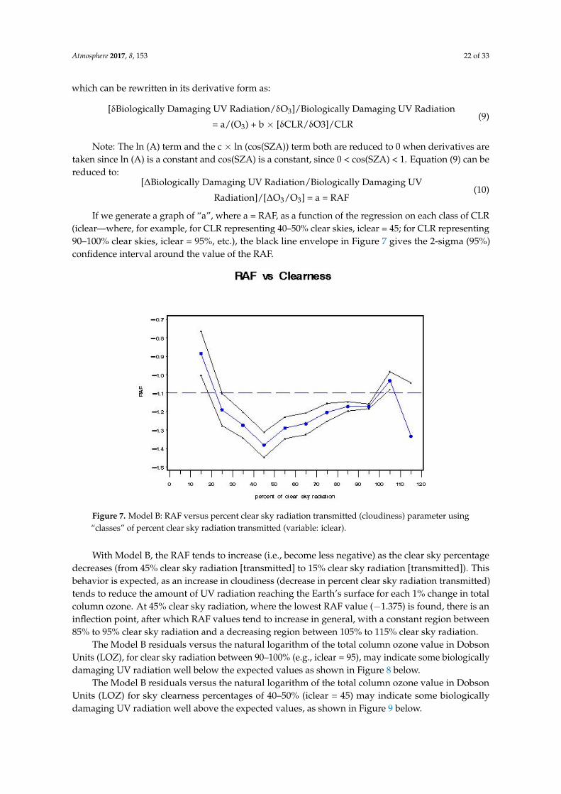
If we generate a graph of “a”, where a = RAF, as a function of the regression on each class of CLR(iclear—where, for example, for CLR representing 40–50% clear skies, iclear = 45; for CLR representing90–100% clear skies, iclear = 95%, etc.), the black line envelope in Figure 7 gives the 2-sigma (95%)confidence interval around the value of the RAF.

Atmosphere 2017, 8, 153 22 of 32


[δBiologically Damaging UV Radiation/δO3]/Biologically Damaging UV Radiation = a/(O3) + b × [δCLR/δO3]/CLR

(9)

Note: The ln (A) term and the c × ln (cos(SZA)) term both are reduced to 0 when derivatives are taken since ln (A) is a constant and cos(SZA) is a constant, since 0 < cos(SZA) < 1. Equation 9 can be reduced to:

[ΔBiologically Damaging UV Radiation/Biologically Damaging UV Radiation]/[ΔO3/O3] = a = RAF

(10)

If we generate a graph of “a”, where a = RAF, as a function of the regression on each class of CLR (iclear—where, for example, for CLR representing 40–50% clear skies, iclear = 45; for CLR representing 90–100% clear skies, iclear = 95%, etc.), the black line envelope in Figure 7 gives the 2-sigma (95%) confidence interval around the value of the RAF.

Figure 7. Model B: RAF versus percent clear sky radiation transmitted (cloudiness) parameter using “classes” of percent clear sky radiation transmitted (variable: iclear).

With Model B, the RAF tends to increase (i.e., become less negative) as the clear sky percentage decreases (from 45% clear sky radiation [transmitted] to 15% clear sky radiation [transmitted]). This behavior is expected, as an increase in cloudiness (decrease in percent clear sky radiation transmitted) tends to reduce the amount of UV radiation reaching the Earth’s surface for each 1% change in total column ozone. At 45% clear sky radiation, where the lowest RAF value (−1.375) is found, there is an inflection point, after which RAF values tend to increase in general, with a constant region between 85% to 95% clear sky radiation and a decreasing region between 105% to 115% clear sky radiation.

The Model B residuals versus the natural logarithm of the total column ozone value in Dobson Units (LOZ), for clear sky radiation between 90–100% (e.g., iclear = 95), may indicate some biologically damaging UV radiation well below the expected values as shown in Figure 8 below.

The Model B residuals versus the natural logarithm of the total column ozone value in Dobson Units (LOZ) for sky clearness percentages of 40–50% (iclear = 45) may indicate some biologically damaging UV radiation well above the expected values, as shown in Figure 9 below.

The residuals for the for sky clearness class 90% to 100% (iclear = 95), Figure 8, and for the sky clearness class 40% to 50% (iclear = 45), Figure 9, would seem to indicate that Model B fits the data well. But note that residuals vs LOZ for iclear = 95 seems to indicate some biologically damaging UV

Figure 7. Model B: RAF versus percent clear sky radiation transmitted (cloudiness) parameter using“classes” of percent clear sky radiation transmitted (variable: iclear).

With Model B, the RAF tends to increase (i.e., become less negative) as the clear sky percentagedecreases (from 45% clear sky radiation [transmitted] to 15% clear sky radiation [transmitted]). Thisbehavior is expected, as an increase in cloudiness (decrease in percent clear sky radiation transmitted)tends to reduce the amount of UV radiation reaching the Earth’s surface for each 1% change in totalcolumn ozone. At 45% clear sky radiation, where the lowest RAF value (−1.375) is found, there is aninflection point, after which RAF values tend to increase in general, with a constant region between85% to 95% clear sky radiation and a decreasing region between 105% to 115% clear sky radiation.

The Model B residuals versus the natural logarithm of the total column ozone value in DobsonUnits (LOZ), for clear sky radiation between 90–100% (e.g., iclear = 95), may indicate some biologicallydamaging UV radiation well below the expected values as shown in Figure 8 below.

The Model B residuals versus the natural logarithm of the total column ozone value in DobsonUnits (LOZ) for sky clearness percentages of 40–50% (iclear = 45) may indicate some biologicallydamaging UV radiation well above the expected values, as shown in Figure 9 below.

Atmosphere 2017, 8, 153 23 of 33

Atmosphere 2017, 8, 153 23 of 32

radiation well below the expected values. The residuals vs LOZ for iclear = 45 may indicate some biologically damaging UV radiation well above the expected values.

The distributions of the biologically damaging UV radiation as shown in Figure 10 are skewed in opposite directions for iclear = 45 (right) and iclear = 95 (left). Partial cloud covering during the measurement of the spectrum (which takes six min to complete) is a potential cause of the skewed biologically damaging UV radiation distributions.

The distributions of the biologically damaging UV radiation as shown in Figure 11 for iclear = 45 and iclear = 95 are less skewed, and closer to normality, for this larger total column ozone range as compared to the total column ozone range (250–280 DU) in Figure 10.

The distributions of the biologically damaging UV radiation as shown in Figure 12 are skewed in opposite directions for iclear = 45 (right) and iclear = 95 (left) for solar zenith angles constrained near 30 degrees.

Figure 8. Model B: Residuals versus the natural logarithm of the total column ozone value in Dobson Units (LOZ) for sky clearness class 90% to 100% (iclear = 95)—Note: LCZA = natural logarithm of the cosine of the solar zenith angle, LDUV = natural logarithm of the biologically damaging UV radiation, and LOZ = natural logarithm of the total column ozone.


Figure 8. Model B: Residuals versus the natural logarithm of the total column ozone value in DobsonUnits (LOZ) for sky clearness class 90% to 100% (iclear = 95)—Note: LCZA = natural logarithm of thecosine of the solar zenith angle, LDUV = natural logarithm of the biologically damaging UV radiation,and LOZ = natural logarithm of the total column ozone.

Atmosphere 2017, 8, 153 23 of 32

radiation well below the expected values. The residuals vs LOZ for iclear = 45 may indicate some biologically damaging UV radiation well above the expected values.

The distributions of the biologically damaging UV radiation as shown in Figure 10 are skewed in opposite directions for iclear = 45 (right) and iclear = 95 (left). Partial cloud covering during the measurement of the spectrum (which takes six min to complete) is a potential cause of the skewed biologically damaging UV radiation distributions.

The distributions of the biologically damaging UV radiation as shown in Figure 11 for iclear = 45 and iclear = 95 are less skewed, and closer to normality, for this larger total column ozone range as compared to the total column ozone range (250–280 DU) in Figure 10.

The distributions of the biologically damaging UV radiation as shown in Figure 12 are skewed in opposite directions for iclear = 45 (right) and iclear = 95 (left) for solar zenith angles constrained near 30 degrees.



Figure 9. Model B: Residuals versus the natural logarithm of the total column ozone value in DobsonUnits (LOZ) for sky clearness class 40% to 50% (iclear = 45)—Note: LCZA = natural logarithm of thecosine of the solar zenith angle, LDUV = natural logarithm of the biologically damaging UV radiation,and LOZ = natural logarithm of the total column ozone.

The residuals for the for sky clearness class 90% to 100% (iclear = 95), Figure 8, and for the skyclearness class 40% to 50% (iclear = 45), Figure 9, would seem to indicate that Model B fits the datawell. But note that residuals vs. LOZ for iclear = 95 seems to indicate some biologically damaging UVradiation well below the expected values. The residuals vs. LOZ for iclear = 45 may indicate somebiologically damaging UV radiation well above the expected values.

The distributions of the biologically damaging UV radiation as shown in Figure 10 are skewedin opposite directions for iclear = 45 (right) and iclear = 95 (left). Partial cloud covering during the

Atmosphere 2017, 8, 153 24 of 33

measurement of the spectrum (which takes six min to complete) is a potential cause of the skewedbiologically damaging UV radiation distributions.Atmosphere 2017, 8, 153 24 of 32

Figure 10. Model B: The biologically damaging UV radiation (adjusted for SZA) for 45% clear skies (green) and 95% clear skies (black) for total column ozone from 250 Dobson Units (DU) to 280 DU—Note: x-axis shows distribution of biologically damaging UV radiation wavelengths seen at 45% clear skies (green) and 95% clear skies (black) and the y-axis shows the percentage of biologically damaging UV radiation at each wavelength range.

Figure 11. Model B: The biologically damaging UV radiation (adjusted for SZA) for 45% clear skies (green) and 95% clear skies (black) for total column ozone from 375 DU to 450 DU—Note: x-axis shows distribution of biologically damaging UV radiation wavelengths seen at 45% clear skies (green) and 95% clear skies (black) and the y-axis shows the percentage of biologically damaging UV radiation at each wavelength range.

Figure 10. Model B: The biologically damaging UV radiation (adjusted for SZA) for 45% clear skies(green) and 95% clear skies (black) for total column ozone from 250 Dobson Units (DU) to 280 DU—Note:x-axis shows distribution of biologically damaging UV radiation wavelengths seen at 45% clear skies(green) and 95% clear skies (black) and the y-axis shows the percentage of biologically damaging UVradiation at each wavelength range.

The distributions of the biologically damaging UV radiation as shown in Figure 11 for iclear = 45and iclear = 95 are less skewed, and closer to normality, for this larger total column ozone range ascompared to the total column ozone range (250–280 DU) in Figure 10.

Atmosphere 2017, 8, 153 24 of 32

Figure 10. Model B: The biologically damaging UV radiation (adjusted for SZA) for 45% clear skies (green) and 95% clear skies (black) for total column ozone from 250 Dobson Units (DU) to 280 DU—Note: x-axis shows distribution of biologically damaging UV radiation wavelengths seen at 45% clear skies (green) and 95% clear skies (black) and the y-axis shows the percentage of biologically damaging UV radiation at each wavelength range.

Figure 11. Model B: The biologically damaging UV radiation (adjusted for SZA) for 45% clear skies (green) and 95% clear skies (black) for total column ozone from 375 DU to 450 DU—Note: x-axis shows distribution of biologically damaging UV radiation wavelengths seen at 45% clear skies (green) and 95% clear skies (black) and the y-axis shows the percentage of biologically damaging UV radiation at each wavelength range.

Figure 11. Model B: The biologically damaging UV radiation (adjusted for SZA) for 45% clear skies(green) and 95% clear skies (black) for total column ozone from 375 DU to 450 DU—Note: x-axis showsdistribution of biologically damaging UV radiation wavelengths seen at 45% clear skies (green) and95% clear skies (black) and the y-axis shows the percentage of biologically damaging UV radiation ateach wavelength range.

Atmosphere 2017, 8, 153 25 of 33

The distributions of the biologically damaging UV radiation as shown in Figure 12 are skewed inopposite directions for iclear = 45 (right) and iclear = 95 (left) for solar zenith angles constrained near30 degrees.Atmosphere 2017, 8, 153 25 of 32

Figure 12. Model B: The biologically damaging UV radiation for 45% clear skies (green) and 95% clear skies (black) for solar zenith angles from 27 degrees to 33 degrees—Note: x-axis shows distribution of biologically damaging UV radiation wavelengths seen at 45% clear skies (green) and 95% clear skies (black) and the y-axis shows the percentage of biologically damaging UV radiation at each wavelength range.

3.1.3. Model C

The relationship between the biologically damaging UV radiation and the following parameters: (1) total column ozone [O3]; (2) “iclear” [Note: to obtain “iclear”, replace the “CLR” term {used in Model A}, with a regression performed on “classes” of CLR; the result of the regression on the “classes” of CLR is called “iclear*”, and remove the tails of the biologically damaging UV radiation distribution, i.e., censor “bad” data; (3) solar zenith angle [SZA], is identical to Model B (using the same equations) except the tails of the biologically damaging UV radiation distributions are removed (data censoring).

If we generate a graph of “a”, where a = RAF, as a function of the regression on each class of CLR (iclear—where, for example, for CLR representing 40–50% clear skies, iclear = 45; for CLR representing 90–100% clear skies, iclear = 95%, etc.), with data censoring (biologically damaging UV radiation distribution tails removed), the black line envelope in Figure 13 gives the 2-sigma (95%) confidence interval around the value of the RAF. When the data in the tails of the biologically damaging UV radiation distributions are removed, there is minimal effect of percent clear sky (cloudiness) on the RAF as compared to Model A or Model B.

With Model C, the RAF tends to increase (i.e., become less negative) as the clear sky percentage decreases (from 25% clear sky radiation [transmitted] to 15% clear sky radiation [transmitted]). This behavior is expected, as an increase in cloudiness (decrease in percent clear sky radiation transmitted) tends to reduce the amount of UV radiation reaching the Earth’s surface for each 1% change in total column ozone. Between 25% and 45% clear sky radiation, there is no visible change in RAF value. This may be a result of the removal of the “tails” of the biologically damaging UV radiation distributions, which would be expected to drive the values of the distributions closer to the mean value. This is the only model without an inflection point at 45% clear sky value, which seems reasonable given the censoring of the tails of the biologically damaging UV radiation distributions. The lowest RAF value (−1.18) occurs at 95% clear sky radiation, which again might be attributable to

Figure 12. Model B: The biologically damaging UV radiation for 45% clear skies (green) and 95% clearskies (black) for solar zenith angles from 27 degrees to 33 degrees—Note: x-axis shows distributionof biologically damaging UV radiation wavelengths seen at 45% clear skies (green) and 95% clearskies (black) and the y-axis shows the percentage of biologically damaging UV radiation at eachwavelength range.

3.1.3. Model C

The relationship between the biologically damaging UV radiation and the following parameters:(1) total column ozone [O3]; (2) “iclear” [Note: to obtain “iclear”, replace the “CLR” term {used inModel A}, with a regression performed on “classes” of CLR; the result of the regression on the “classes”of CLR is called “iclear*”, and remove the tails of the biologically damaging UV radiation distribution,i.e., censor “bad” data; (3) solar zenith angle [SZA], is identical to Model B (using the same equations)except the tails of the biologically damaging UV radiation distributions are removed (data censoring).

If we generate a graph of “a”, where a = RAF, as a function of the regression on each class of CLR(iclear—where, for example, for CLR representing 40–50% clear skies, iclear = 45; for CLR representing90–100% clear skies, iclear = 95%, etc.), with data censoring (biologically damaging UV radiationdistribution tails removed), the black line envelope in Figure 13 gives the 2-sigma (95%) confidenceinterval around the value of the RAF. When the data in the tails of the biologically damaging UVradiation distributions are removed, there is minimal effect of percent clear sky (cloudiness) on theRAF as compared to Model A or Model B.

With Model C, the RAF tends to increase (i.e., become less negative) as the clear sky percentagedecreases (from 25% clear sky radiation [transmitted] to 15% clear sky radiation [transmitted]). Thisbehavior is expected, as an increase in cloudiness (decrease in percent clear sky radiation transmitted)tends to reduce the amount of UV radiation reaching the Earth’s surface for each 1% change in totalcolumn ozone. Between 25% and 45% clear sky radiation, there is no visible change in RAF value. This

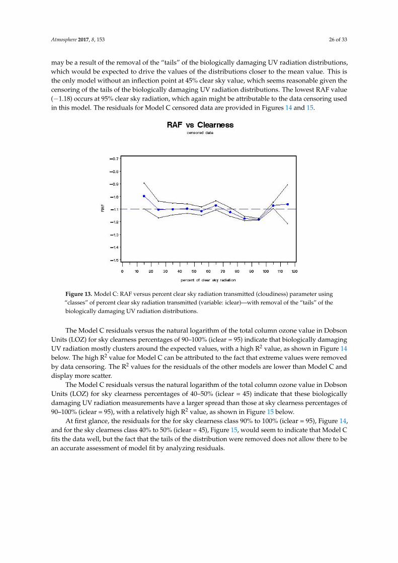
Atmosphere 2017, 8, 153 26 of 33

may be a result of the removal of the “tails” of the biologically damaging UV radiation distributions,which would be expected to drive the values of the distributions closer to the mean value. This isthe only model without an inflection point at 45% clear sky value, which seems reasonable given thecensoring of the tails of the biologically damaging UV radiation distributions. The lowest RAF value(−1.18) occurs at 95% clear sky radiation, which again might be attributable to the data censoring usedin this model. The residuals for Model C censored data are provided in Figures 14 and 15.

Atmosphere 2017, 8, 153 26 of 32

the data censoring used in this model. The residuals for Model C censored data are provided in Figures 14 and 15.

Figure 13. Model C: RAF versus percent clear sky radiation transmitted (cloudiness) parameter using “classes” of percent clear sky radiation transmitted (variable: iclear)—with removal of the “tails” of the biologically damaging UV radiation distributions.

The Model C residuals versus the natural logarithm of the total column ozone value in Dobson Units (LOZ) for sky clearness percentages of 90–100% (iclear = 95) indicate that biologically damaging UV radiation mostly clusters around the expected values, with a high R2 value, as shown in Figure 14 below. The high R2 value for Model C can be attributed to the fact that extreme values were removed by data censoring. The R2 values for the residuals of the other models are lower than Model C and display more scatter.

Figure 14. Model C: Residuals versus the natural logarithm of the total column ozone value in Dobson Units (LOZ) for sky clearness class 90% to 100% (iclear = 95) with removal of the “tails” of the biologically damaging UV radiation distributions—Note: LCZA = natural logarithm of the cosine of the solar zenith angle, LDUV = natural logarithm of the biologically damaging UV radiation, and LOZ = natural logarithm of the total column ozone.

Figure 13. Model C: RAF versus percent clear sky radiation transmitted (cloudiness) parameter using“classes” of percent clear sky radiation transmitted (variable: iclear)—with removal of the “tails” of thebiologically damaging UV radiation distributions.

The Model C residuals versus the natural logarithm of the total column ozone value in DobsonUnits (LOZ) for sky clearness percentages of 90–100% (iclear = 95) indicate that biologically damagingUV radiation mostly clusters around the expected values, with a high R2 value, as shown in Figure 14below. The high R2 value for Model C can be attributed to the fact that extreme values were removedby data censoring. The R2 values for the residuals of the other models are lower than Model C anddisplay more scatter.

The Model C residuals versus the natural logarithm of the total column ozone value in DobsonUnits (LOZ) for sky clearness percentages of 40–50% (iclear = 45) indicate that these biologicallydamaging UV radiation measurements have a larger spread than those at sky clearness percentages of90–100% (iclear = 95), with a relatively high R2 value, as shown in Figure 15 below.

At first glance, the residuals for the for sky clearness class 90% to 100% (iclear = 95), Figure 14,and for the sky clearness class 40% to 50% (iclear = 45), Figure 15, would seem to indicate that Model Cfits the data well, but the fact that the tails of the distribution were removed does not allow there to bean accurate assessment of model fit by analyzing residuals.

Atmosphere 2017, 8, 153 27 of 33

Atmosphere 2017, 8, 153 26 of 32

the data censoring used in this model. The residuals for Model C censored data are provided in Figures 14 and 15.

Figure 13. Model C: RAF versus percent clear sky radiation transmitted (cloudiness) parameter using “classes” of percent clear sky radiation transmitted (variable: iclear)—with removal of the “tails” of the biologically damaging UV radiation distributions.

The Model C residuals versus the natural logarithm of the total column ozone value in Dobson Units (LOZ) for sky clearness percentages of 90–100% (iclear = 95) indicate that biologically damaging UV radiation mostly clusters around the expected values, with a high R2 value, as shown in Figure 14 below. The high R2 value for Model C can be attributed to the fact that extreme values were removed by data censoring. The R2 values for the residuals of the other models are lower than Model C and display more scatter.


Figure 14. Model C: Residuals versus the natural logarithm of the total column ozone value inDobson Units (LOZ) for sky clearness class 90% to 100% (iclear = 95) with removal of the “tails” ofthe biologically damaging UV radiation distributions—Note: LCZA = natural logarithm of the cosineof the solar zenith angle, LDUV = natural logarithm of the biologically damaging UV radiation, andLOZ = natural logarithm of the total column ozone.

Atmosphere 2017, 8, 153 27 of 32

The Model C residuals versus the natural logarithm of the total column ozone value in Dobson Units (LOZ) for sky clearness percentages of 40–50% (iclear = 45) indicate that these biologically damaging UV radiation measurements have a larger spread than those at sky clearness percentages of 90–100% (iclear = 95), with a relatively high R2 value, as shown in Figure 15 below.


At first glance, the residuals for the for sky clearness class 90% to 100% (iclear = 95), Figure 14, and for the sky clearness class 40% to 50% (iclear = 45), Figure 15, would seem to indicate that Model C fits the data well, but the fact that the tails of the distribution were removed does not allow there to be an accurate assessment of model fit by analyzing residuals.

3.1.4. Model D

The relationship between the biologically damaging UV radiation and the following parameters: (1) total column ozone [O3]; (2) CLR^ [assuming a linear function in percent clearness {“classes” of CLR} for skies between 40% clear and 100% clear]; (3) solar zenith angle [SZA], is given as follows:

Biologically Damaging UV Radiation = A × (O3)a + b × CLR^ × (cos(SZA))c (11)

where a + b × CLR^ represents a linear function in percent clearness for 40–100% clear skies. The slope of the UVR–ozone relationships derived for clear skies, light cloudy skies, medium

cloudy skies and heavy cloudy skies for this model, can be found using the formula:

ln (Biologically Damaging UV Radiation) = ln(A) + a × ln (O3) + b × CLR^ × ln (O3) + c × ln(cos(SZA)) (12)


[δBiologically Damaging UV Radiation/δO3]/Biologically Damaging UV Radiation = (a + b × CLR^)/(O3)

(13)

Note: The ln (A) term and the c × ln (cos(SZA)) term both are reduced to 0 when derivatives are taken since ln (A) is a constant and cos(SZA) is a constant, since 0 < cos(SZA) < 1. Equation 13 can be reduced to:

Figure 15. Model C: Residuals versus the natural logarithm of the total column ozone value in DobsonUnits (LOZ) for sky clearness class 40% to 50% (iclear = 45) with removal of the “tails” of the biologicallydamaging UV radiation distributions—Note: LCZA = natural logarithm of the cosine of the solarzenith angle, LDUV = natural logarithm of the biologically damaging UV radiation, and LOZ = naturallogarithm of the total column ozone.

3.1.4. Model D

The relationship between the biologically damaging UV radiation and the following parameters:(1) total column ozone [O3]; (2) CLRˆ [assuming a linear function in percent clearness {“classes” ofCLR} for skies between 40% clear and 100% clear]; (3) solar zenith angle [SZA], is given as follows:

Biologically Damaging UV Radiation = A × (O3)a + b × CLRˆ × (cos(SZA))c (11)

Atmosphere 2017, 8, 153 28 of 33

where a + b × CLRˆ represents a linear function in percent clearness for 40–100% clear skies.The slope of the UVR–ozone relationships derived for clear skies, light cloudy skies, medium

cloudy skies and heavy cloudy skies for this model, can be found using the formula:

ln (Biologically Damaging UV Radiation) = ln(A) + a × ln (O3) + b × CLRˆ × ln (O3) +

c × ln(cos(SZA))(12)



= (a + b × CLRˆ)/(O3)(13)

Note: The ln (A) term and the c × ln (cos(SZA)) term both are reduced to 0 when derivatives aretaken since ln (A) is a constant and cos(SZA) is a constant, since 0 < cos(SZA) < 1. Equation (13) can bereduced to:

[∆Biologically Damaging UV Radiation/Biologically Damaging UV Radiation] [∆O3/O3]

= (a + b × CLRˆ) = RAF(14)

The black line envelope in Figure 16 gives the 2-sigma (95%) confidence interval around the valueof the RAF. The results were similar to those found in Model B for individual regressions using the“iclear*” parameter to represent classes of percent clearness. Note in Figure 16 the “dip” in RAF valuesbetween 45–55% clearness. This could indicate isolated clouds passing over the sun during individualmeasurement scan periods.

Atmosphere 2017, 8, 153 28 of 32

[ΔBiologically Damaging UV Radiation/Biologically Damaging UV Radiation] [ΔO3/O3] = (a + b × CLR^) = RAF

(14)

The black line envelope in Figure 16 gives the 2-sigma (95%) confidence interval around the value of the RAF. The results were similar to those found in Model B for individual regressions using the “iclear*” parameter to represent classes of percent clearness. Note in Figure 16 the “dip” in RAF values between 45–55% clearness. This could indicate isolated clouds passing over the sun during individual measurement scan periods.

Figure 16. Model D: RAF versus percent clear sky radiation transmitted (cloudiness) parameter (CLR^): a linear function between 40% and 100% clear sky radiation transmitted.

With Model D, the RAF tends to increase (i.e., become less negative) as the clear sky percentage decreases (from 45% clear sky radiation [transmitted] to 15% clear sky radiation [transmitted]). This behavior is expected, as an increase in cloudiness (decrease in percent clear sky radiation transmitted) tends to reduce the amount of UV radiation reaching the Earth’s surface for each 1% change in total column ozone. At 45% clear sky radiation, where the lowest RAF value (−1.3) is found, there is an inflection point, after which RAF values increase, with one exception between 85% to 95% clear sky radiation. The RAF values between 40–60% clear sky radiation could possibly indicate an isolated cloud over the sun during a scan.

3.1.5. Model E—(A Model Based on an Empirical Relationship: Beer–Lambert’s Law)

The functional relationship between the biologically damaging UV radiation and the following parameters: total column ozone [O3]/cos(SZA), and cos(SZA), based on Beer–Lambert’s Law is shown in Equation 15 (where k = −RAF/{O3/cos(SZA)}):

Biologically Damaging UV Radiation = A × exp (−k × O3/cos(SZA)) × (cos(SZA))c (15)

The slope of the UVR–ozone relationships derived for clear skies, light cloudy skies, medium cloudy skies and heavy cloudy skies for this model, can be found using Equation 16:

ln (Biologically Damaging UV Radiation) = ln (A)−k × O3/cos(SZA) + c × ln (cos(SZA))

(16)


[δBiologically Damaging UV Radiation/δO3]/Biologically Damaging UV Radiation =−k × O3/cos(SZA) (17)

Figure 16. Model D: RAF versus percent clear sky radiation transmitted (cloudiness) parameter (CLRˆ):a linear function between 40% and 100% clear sky radiation transmitted.

With Model D, the RAF tends to increase (i.e., become less negative) as the clear sky percentagedecreases (from 45% clear sky radiation [transmitted] to 15% clear sky radiation [transmitted]). Thisbehavior is expected, as an increase in cloudiness (decrease in percent clear sky radiation transmitted)tends to reduce the amount of UV radiation reaching the Earth’s surface for each 1% change in totalcolumn ozone. At 45% clear sky radiation, where the lowest RAF value (−1.3) is found, there isan inflection point, after which RAF values increase, with one exception between 85–95% clear sky

Atmosphere 2017, 8, 153 29 of 33

radiation. The RAF values between 40–60% clear sky radiation could possibly indicate an isolatedcloud over the sun during a scan.

3.1.5. Model E—(A Model Based on an Empirical Relationship: Beer–Lambert’s Law)

The functional relationship between the biologically damaging UV radiation and the followingparameters: total column ozone [O3]/cos(SZA), and cos(SZA), based on Beer–Lambert’s Law is shownin Equation (15) (where k = −RAF/{O3/cos(SZA)}):

Biologically Damaging UV Radiation = A × exp (−k × O3/cos(SZA)) × (cos(SZA))c (15)

The slope of the UVR–ozone relationships derived for clear skies, light cloudy skies, mediumcloudy skies and heavy cloudy skies for this model, can be found using Equation (16):

ln (Biologically Damaging UV Radiation) = ln (A)−k × O3/cos(SZA) + c × ln (cos(SZA)) (16)

Which can be rewritten in its derivative form as:


= −k × O3/cos(SZA)(17)

Note: The ln (A) term and the c × ln (cos(SZA)) term both are reduced to 0 when derivatives aretaken since ln (A) is a constant and cos (SZA) is a constant, since 0 < cos(SZA) < 1. Equation (17) can bereduced to:

[∆Biologically Damaging UV Radiation/Biologically Damaging UV Radiation]/[∆O3/O3]

=−k × O3/cos(SZA) = RAF(18)

Using fixed values for average total column ozone and average solar zenith angle facilitatessensitivity analysis of the RAF.

RAF =−k × avg O3/cos(avg SZA): [avg O3 = 315 DU, avg SZA = 36 deg] (19)

In order to make the definition of UV-A temporally closer to the definition of the biologicallydamaging UV radiation, for this model (Model E), use the UVR wavelength range of 325–330 nm{UV325: Figure 3}, which is unaffected by ozone, not 330–363 nm (Figure 5) used previously inModels A through D. Since the empirical relationship is proportional to total column ozone, it isnecessary to find the portion of the electromagnetic spectrum where UVR is unaffected by atmosphericozone and observe the variation of SZA and cloudiness on biologically damaging UV radiation. Theblack line envelope in Figure 17 gives the 2-sigma (95%) confidence interval around the value ofthe RAF. Beer–Lambert’s Law suggests that a more suitable physical model implies that the RAF isnot constant but is proportional to (O3/cos(SZA)). However, using average ozone and SZA valuesyielded results similar to those provided in Figure 17. Note in Figure 17 the “dip” in RAF valuesbetween 40–50% clearness. This could indicate isolated clouds passing over the sun during individualmeasurement scan periods. Note: There may be a relationship between the seasonal ozone cycle(i.e., high ozone = spring, low ozone = fall), cloud types, and cloud coverage amounts requiringfurther exploration.

With Model E, the RAF tends to increase (i.e., become less negative) as the clear sky percentagedecreases (from 45% clear sky radiation [transmitted] to 15% clear sky radiation [transmitted]). Thisbehavior is expected, as an increase in cloudiness (decrease in percent clear sky radiation transmitted)tends to reduce the amount of UV radiation reaching the Earth’s surface for each 1% change in totalcolumn ozone. At 45% clear sky radiation, where the lowest RAF value (−1.28) is found, there is an

Atmosphere 2017, 8, 153 30 of 33

inflection point, after which RAF values increase, with exceptions between 75% and 85% clear skyradiation, and between 105% and 115% clear sky radiation, consistent with [22].

Atmosphere 2017, 8, 153 29 of 32

Note: The ln (A) term and the c × ln (cos(SZA)) term both are reduced to 0 when derivatives are taken since ln (A) is a constant and cos (SZA) is a constant, since 0 < cos(SZA) < 1. Equation 17 can be reduced to:

[ΔBiologically Damaging UV Radiation/Biologically Damaging UV Radiation]/[ΔO3/O3] =−k × O3/cos(SZA) = RAF (18)

Using fixed values for average total column ozone and average solar zenith angle facilitates sensitivity analysis of the RAF.

RAF =−k × avg O3/cos(avg SZA): [avg O3 = 315 DU, avg SZA = 36 deg] (19)

In order to make the definition of UV-A temporally closer to the definition of the biologically damaging UV radiation, for this model (Model E), use the UVR wavelength range of 325–330 nm {UV325: Figures 3}, which is unaffected by ozone, not 330–363 nm (Figures 5) used previously in Models A through D. Since the empirical relationship is proportional to total column ozone, it is necessary to find the portion of the electromagnetic spectrum where UVR is unaffected by atmospheric ozone and observe the variation of SZA and cloudiness on biologically damaging UV radiation. The black line envelope in Figure 17 gives the 2-sigma (95%) confidence interval around the value of the RAF. Beer–Lambert’s Law suggests that a more suitable physical model implies that the RAF is not constant but is proportional to (O3/cos(SZA)). However, using average ozone and SZA values yielded results similar to those provided in Figure 17. Note in Figure 17 the “dip” in RAF values between 40–50% clearness. This could indicate isolated clouds passing over the sun during individual measurement scan periods. Note: There may be a relationship between the seasonal ozone cycle (i.e., high ozone = spring, low ozone = fall), cloud types, and cloud coverage amounts requiring further exploration.

Figure 17. Model E: RAF versus percent clear sky radiation transmitted (cloudiness) parameter: {O3/cos(SZA)/cos(SZA)}.

With Model E, the RAF tends to increase (i.e., become less negative) as the clear sky percentage decreases (from 45% clear sky radiation [transmitted] to 15% clear sky radiation [transmitted]). This behavior is expected, as an increase in cloudiness (decrease in percent clear sky radiation transmitted) tends to reduce the amount of UV radiation reaching the Earth’s surface for each 1% change in total column ozone. At 45% clear sky radiation, where the lowest RAF value (−1.28) is found, there is an inflection point, after which RAF values increase, with exceptions between 75% and 85% clear sky radiation, and between 105% and 115% clear sky radiation, consistent with [22].

Although Model A and Model B have average RAF values closer to −1.2, while Model D has an average value of nearly −1.1 (−1.087), Model A, Model B, and Model D behave in a similar fashion, as

Figure 17. Model E: RAF versus percent clear sky radiation transmitted (cloudiness) parameter:{O3/cos(SZA)/cos(SZA)}.

Although Model A and Model B have average RAF values closer to −1.2, while Model D has anaverage value of nearly −1.1 (−1.087), Model A, Model B, and Model D behave in a similar fashion,as they each display the relationship where RAF decreases as clear sky increases (percent cloudinessdecreases) between the 100% to 120% clear sky values. Each of these three models displays thelowest RAF values (−1.3 to −1.38) at the 45% clear sky value. Due to the censoring of the tails of thebiologically damaging UV radiation distribution, understandably, Model C has a “flattened” RAFversus clear sky response curve. Model E, like Model A, Model B, and Model D, also has its lowestRAF value (−1.28) at the 45% clear sky value. The average RAF value of Model E is −1.119 (lessthan Model A), and it displays the relationship where RAF increases as clear sky increases (percentcloudiness decreases) between the 85% to 105% clear sky values, unlike Models A, B, and D.

4. Conclusions

This research project utilized a large dataset of UVR measurements from ten monitoring sites thatwere diverse with respect to spatial location, geography, climate, altitude, and ecology to calculateRAF using four hypothetical approaches and one empirical model. This research project developeda consistent definition of cloudiness, independent of total column ozone, and temporally close tobiologically damaging UV radiation measurements to facilitate direct and consistent comparisonsbetween each of the approaches for modeling RAF. Model C, which censors the tails of the biologicallydamaging UV radiation distribution, should not be used to assess RAF, since the RAF value isartificially driven to a mean value (−1.1). While Models A, B, and D are consistent and comparable inthe relationship between RAF and clear sky radiation between 100% and 120%, the empirically-basedmodel, Model E, behaves differently in that range.

The results show that for all models except Model C (censored tails), in the 35% to 65% range ofclear sky radiation (65% to 35% cloudiness), as cloudiness decreases, RAF increases, ranging from −1.2to −1.4, where it reaches its highest level before decreasing. Between 15% and 25% clear sky radiation(85% to 75% cloudiness), there is an increase in RAF for all models. In general, RAF tends to increaseas the sky conditions change from high to moderate cloudiness. Clouds block biologically damagingUV radiation in this range and the behavior is qualitatively the same as if stratospheric ozone was

Atmosphere 2017, 8, 153 31 of 33

increased. UVR can experience a 4.3% increase per kilometer of altitude, from 0 km to 6.2 km, and isalso affected by atmospheric pressure and aerosol density [23]. It is noted in the literature that meancloud attenuation of UVR in the UV-B (wavelengths: 280–315 nm) is approximately 15–30% [24]. UVradiation is also reflected by both clouds and the Earth’s surface [25], which complicates analyses inthis area. Erythemally-weighted UV-B has displayed a 3–7% decadal increase in mid and high latitudesfrom Nimbus 7 satellite observations [26]. For 105% to 120% clear sky radiation, RAF increases forModels A, B and E, while decreasing for Models C and D. The RAF is important because it serves asa sensitivity metric that directly relates changes in stratospheric ozone to changes in the UVR fluxreaching the Earth’s surface. Overall, the resulting RAF values from the five modeling approaches areconsistent with those found in [27].

Acknowledgments: The author appreciates the advice and guidance on this manuscript from Symielle A. Gastonand Timothy M. Barzyk from the US EPA Office of Research and Development (ORD) National Exposure ResearchLaboratory (NERL). The author gives special thanks to Jack H. Shreffler, US EPA ORD/NERL (retired), who laidthe foundation for this research and was an understanding mentor.

Author Contributions: Eric S. Hall is solely responsible for the development of this manuscript, the analysis, andinterpretation of the results.

Conflicts of Interest: The author declares no conflict of interest. The United States Environmental ProtectionAgency through its office of Research and Development funded and managed the research described here undercontract 68-D-04-001 with the University of Georgia at Athens (UGA); partially funded through InteragencyAgreement Number DW13921546-01 in collaboration with the National Institute for Standards and Technology(NIST); partially funded through Interagency Agreement Number DW139392300-01 in collaboration with theNational Oceanic and Atmospheric Administration (NOAA); and partially funded through Interagency AgreementNumber DW14939466-01-0 in collaboration with the National Parks Service (NPS). It has been subjected to theAgency review and approved for publication. Although this work was reviewed by U.S. EPA and approved forpublication, it may not necessarily reflect official Agency policy. Mention of trade names or commercial productsdoes not constitute endorsement or recommendation for use.

Abbreviations

CCD charge-coupled deviceCFC chlorofluorocarbonCLR percent clear sky radiationDOI US Department of the InteriorDOS disk operating systemDU Dobson UnitDUV biologically damaging UV radiationEPA US Environmental Protection AgencyGMT Greenwich Mean TimeIAG Interagency AgreementLCZA natural logarithm of the cosine of the solar zenith angleLDUV natural logarithm of the biologically damaging UV radiationLOZ natural logarithm of the total column ozonePCLR fraction of clear sky radiationNASA National Aeronautics and Space AdministrationNERL EPA National Exposure Research LaboratoryNIST US National Institute for Standards and TechnologyNOAA National Oceanographic and Atmospheric AdministrationNUVMC National UV Monitoring CenterNPS US National Parks ServiceO3 total column ozoneORD EPA Office of Research and DevelopmentRAF Radiation Amplification FactorSZA Solar Zenith AngleTOMS NASA Total Ozone Mapping SpectrometerUGA University of Georgia at AthensUS United StatesUV ultravioletUVR ultraviolet radiation

Atmosphere 2017, 8, 153 32 of 33

References

1. Gerstl, S.A.W.; Zardecki, A.; Wiser, H.L. Biologically damaging radiation amplified by ozone depletions.Nature 1981, 294, 352–354. [CrossRef]

2. Smertenko, P.; Stepanov, V.; Ol’khovik, C.; Durzan, D.J. New approach to a radiation amplification factor.In Cell Biology and Instrumentation: UV Radiation, Nitric Oxide, and Cell Death in Plants; Blume, Y., Durzan, D.J.,Smertenko, P., Eds.; IOS Press: Amsterdam, The Netherlands, 2006; ISBN 1-58603-574-6.

3. Parisi, A.V.; Sabburg, J.; Kimlin, M.G. Scattered and Filtered Solar UV Measurements; Kluwer AcademicPublishers: Dordrecht, The Netherlands, 2004.

4. Madronich, S.; McKenzie, R.L.; Bjorn, L.O.; Caldwell, M.M. Changes in biologically active ultravioletradiation reaching the Earth’s surface. J. Photochem. Photobiol. B 1998, 46, 5–19. [CrossRef]

5. Pfister, G.; McKenzie, R.L.; Liley, J.B.; Thomas, A.; Forgan, B.W.; Long, C.N. Cloud coverage based on all-skyimaging and its impact on surface solar irradiance. J. Appl. Meteorol. Clim. 2003, 42, 1421–1434. [CrossRef]

6. Hall, E.S. Ground-Based Measurement of Solar Ultraviolet Radiation. In McGraw-Hill Yearbook of Science andTechnology; Kotowski, F., Jr., Ed.; McGraw-Hill Book Co.: New York, NY, USA, 2009; pp. 150–155.

7. Sabburg, J. EPA/UGA, UV/QA Data Correction Project Specification (v2.3); Unpublished work, 2001.8. Weatherhead, E.C.; Frederick, J.E. Report on Geographic and Seasonal Variability of UV Affecting Human and

Ecological Health. Available online: https://cfpub.epa.gov/si/si_public_record_Report.cfm?dirEntryID=133325 (accessed on 17 August 2017).

9. Lenoble, J. Atmospheric Radiation Transfer; A. Deepak Publishing: Hampton, VA, USA, 1993.10. Warhaft, Z. An Introduction to Thermal-Fluid Engineering: The Engine and the Atmosphere; Cambridge University

Press: Cambridge, UK, 1997; ISBN 0-521-58100-1.11. Frederick, J.E.; Snell, H.E.; Haywood, E.K. Solar ultraviolet radiation at the earth’s surface. Photochem.

Photobiol. 1989, 50, 443–450. [CrossRef]12. Crist, K.C.; Carmichael, G.R.; John, K. UV-B exposure and atmospheric ozone: Evaluation of radiative flux to

changes in ambient ozone levels. J. Hazard. Mater. 1994, 37, 527–538. [CrossRef]13. Sivasakthivel, T.; Reddy, K.S.K. Ozone Layer Depletion and Its Effects: A Review. Available online: http:

//www.ijesd.org/papers/93-D500.pdf (accessed on 17 August 2017).14. Rowland, F.S. Stratospheric Ozone Depletion. Philos. T. Roy. Soc. B 2006, 361, 769–790. [CrossRef] [PubMed]15. McCulloch, A.; Midgley, P.M.; Ashford, P. Releases of refrigerant gases (CFC-12, HCFC-22, and HFC-134a) to

the atmosphere. Atmos. Environ. 2003, 37, 889–902. [CrossRef]16. United Nations Environment Programme (UNEP). The 1987 Montreal Protocol on Substances that Deplete

the Ozone Layer. Available online: http://ozone.unep.org/new_site/en/Treaties/treaties_decisions-hb.php?sec_id=342&show_all (accessed on 17 August 2017).

17. US Environmental Protection Agency (US EPA). Clean Air Act Title VI—Stratospheric Ozone Protection.42 USC 7671 (Title 42 [The Public Health and Welfare], Chapter 85 [Air Pollution Prevention and Control],Subchapter VI [Stratospheric Ozone Protection]). Available online: https://www.epa.gov/clean-air-act-overview/clean-air-act-title-vi-stratospheric-ozone-protection (accessed on 4 August 2017).

18. Brewer MKIV Spectrophotometer Operator’s Manual. Available online: https://www.esrl.noaa.gov/gmd/grad/neubrew/docs/manuals/Brewer_MkIV_service_manual.pdf (accessed on 17 August 2017).

19. Binyamin, J.; Davies, J.; McArthur, B. Validation of spectral and broadband UV-B (290–325 nm) irradiance forCanada. Atmos. Clim. Sci. 2011, 1, 69–85. [CrossRef]

20. Feister, U.; Cabrol, N.; Häder, D. UV enhancements by scattering of solar radiation from clouds. Atmosphere2015, 6, 1211–1228. [CrossRef]

21. ITACA. The Sun as a Source of Energy, Part 4: Irradiation Calculations. Available online: http://www.itacanet.org/the-sun-as-a-source-of-energy/part-4-irradiation-calculations/ (accessed on 17 August 2017).

22. El-Nouby, A.M. Effect of stratospheric ozone in UVB solar radiation reaching the Earth’s surface at Qena,Egypt. Atmos. Pollut. Res. 2010, 1, 155–160. [CrossRef]

23. Varotsos, C. Airborne measurements of aerosol, ozone, and solar ultraviolet irradiance in the troposphere.J. Geophys. Res. Atmos. 2005, 110, 2156–2202. [CrossRef]

24. Mckenzie, R.L.; Bjorn, L.O.; Bais, A.; Ilyas, M. Changes in biologically active ultraviolet radiation reachingthe Earth’s surface. Photochem. Photobiol. Sci. 2003, 2, 5–15. [CrossRef] [PubMed]

http://dx.doi.org/10.1038/294352a0

http://dx.doi.org/10.1016/S1011-1344(98)00182-1

http://dx.doi.org/10.1175/1520-0450(2003)042<1421:CCBOAI>2.0.CO;2

https://cfpub.epa.gov/si/si_public_record_Report.cfm?dirEntryID=133325

https://cfpub.epa.gov/si/si_public_record_Report.cfm?dirEntryID=133325

http://dx.doi.org/10.1111/j.1751-1097.1989.tb05548.x

http://dx.doi.org/10.1016/0304-3894(93)E0096-K

http://www.ijesd.org/papers/93-D500.pdf

http://www.ijesd.org/papers/93-D500.pdf

http://dx.doi.org/10.1098/rstb.2005.1783

http://www.ncbi.nlm.nih.gov/pubmed/16627294

http://dx.doi.org/10.1016/S1352-2310(02)00975-5

http://ozone.unep.org/new_site/en/Treaties/treaties_decisions-hb.php?sec_id=342&show_all

http://ozone.unep.org/new_site/en/Treaties/treaties_decisions-hb.php?sec_id=342&show_all

https://www.epa.gov/clean-air-act-overview/clean-air-act-title-vi-stratospheric-ozone-protection

https://www.epa.gov/clean-air-act-overview/clean-air-act-title-vi-stratospheric-ozone-protection

https://www.esrl.noaa.gov/gmd/grad/neubrew/docs/manuals/Brewer_MkIV_service_manual.pdf

https://www.esrl.noaa.gov/gmd/grad/neubrew/docs/manuals/Brewer_MkIV_service_manual.pdf

http://dx.doi.org/10.4236/acs.2011.13008

http://dx.doi.org/10.3390/atmos6081211

http://www.itacanet.org/the-sun-as-a-source-of-energy/part-4-irradiation-calculations/

http://www.itacanet.org/the-sun-as-a-source-of-energy/part-4-irradiation-calculations/

http://dx.doi.org/10.5094/APR.2010.020

http://dx.doi.org/10.1029/2004JD005397

http://dx.doi.org/10.1039/B211155C


Atmosphere 2017, 8, 153 33 of 33

25. McKenzie, R.L.; Aucamp, P.J.; Bais, A.F.; Björn, L.O.; Ilyas, M. Changes in biologically active ultravioletradiation reaching the Earth’s surface. Photochem. Photobiol. Sci. 2007, 6, 218–231. [CrossRef] [PubMed]

26. Ziemke, J.R.; Chandra, S.; Herman, J.; Varotsos, C. Erythemally weighted UV trends over northern latitudesderived from Nimbus 7 TOMS measurements. J. Geophys. Res. Atmos. 2000, 105, 7373–7382. [CrossRef]

27. Massen, F. Computing the Radiation Amplification Factor RAF Using a Sudden Dip in Total Ozone ColumnMeasured at Diekirch, Luxembourg. Available online: http://meteo.lcd.lu/papers/MASSEN/RAF_from_sudden_TOC_dip.pdf (accessed on 17 August 2017).

© 2017 by the author. Licensee MDPI, Basel, Switzerland. This article is an open accessarticle distributed under the terms and conditions of the Creative Commons Attribution(CC BY) license (http://creativecommons.org/licenses/by/4.0/).

http://dx.doi.org/10.1039/B700017K


http://dx.doi.org/10.1029/1999JD901131

http://meteo.lcd.lu/papers/MASSEN/RAF_from_sudden_TOC_dip.pdf

http://meteo.lcd.lu/papers/MASSEN/RAF_from_sudden_TOC_dip.pdf

http://creativecommons.org/

http://creativecommons.org/licenses/by/4.0/.

Comparison of Five Modeling Approaches to Quantify and ...

Documents

Transcript of Comparison of Five Modeling Approaches to Quantify and ...