Comparison of Continuous and Discontinuous Galerkin Approaches ...

Zeitschrift fur Angewandte Mathematik und Mechanik, 24 August 2015

Comparison of Continuous and Discontinuous Galerkin Approaches forVariable-Viscosity Stokes Flow

Ragnar S. Lehmann1,2∗, Maria Lukacova-Medvid’ova1,3, Boris J. P. Kaus1,2, and Anton A. Popov2

1 Max Planck Graduate Center with the Johannes Gutenberg-Universitat Mainz (MPGC), Germany2 Institute of Geosciences, Johannes Gutenberg-Universitat Mainz, Germany3 Institute of Mathematics, Johannes Gutenberg-Universitat Mainz, Germany

Received XXXX, revised XXXX, accepted XXXXPublished online XXXX

Key words variable-viscosity Stokes Flow, Discontinuous Galerkin, Finite Element Method, Computational Fluid Dy-namics, mixed methods, Computational Geodynamics, incompressible fluid flow, divergence-conforming elements.MSC (2010) 04A25

We describe a Discontinuous Galerkin (DG) scheme for variable-viscosity Stokes flow which is a crucial aspect of manygeophysical modelling applications and conduct numerical experiments with different elements comparing the DG ap-proach to the standard Finite Element Method (FEM). We compare the divergence-conforming lowest-order Raviart-Thomas (RT0P0) and Brezzi-Douglas-Marini (BDM1P0) element in the DG scheme with the bilinear Q1P0 and biquadraticQ2P1 elements for velocity and their matching piecewise constant/linear elements for pressure in the standard continuousGalerkin (CG) scheme with respect to accuracy and memory usage in 2D benchmark setups.

We find that for the chosen geodynamic benchmark setups the DG scheme with the BDM1P0 element gives the expectedconvergence rates and accuracy but has (for fixed mesh) higher memory requirements than the CG scheme with the Q1P0

element without yielding significantly higher accuracy. The DG scheme with the RT0P0 element is cheaper than the otherfirst-order elements and yields almost the same accuracy in simple cases but does not converge for setups with non-zeroshear stress. The known instability modes of the Q1P0 element did not play a role in the tested setups leading to theBDM1P0 and Q1P0 elements being equally reliable. Not only for a fixed mesh resolution, but also for fixed memorylimitations, using a second-order element like Q2P1 gives higher accuracy than the considered first-order elements.

Copyright line will be provided by the publisher

1 Introduction and Geophysical Motivation

Numerical simulations of geological and geodynamic processes is an important and growing research field which helps tointerprete geological observations in a physically meaningful manner. Typical questions that are addressed include: Howare sedimentary basins formed (e.g., [1])? How do lithospheric plates collide and how are mountains formed (e.g., [2–5])?Why do we have plate tectonics on Earth and not on other planets (e.g., [6,7])? What is the rheology of magma [8] and howdoes magma move through the Earth and why does it only sometimes result in volcanic eruptions [9]? How does mantleconvection work [7], and was this different in the early Earth [10]? While the rheology of rocks is rather complex andnonlinear and is best described as viscoelastoplastic, inertial terms are not important for these processes and the governingequations that need to be solved in this case are often very similar to the incompressible Stokes equations [7, 11–14].Yet, different than in many classical CFD applications, geological processes have viscosities that vary by many orders ofmagnitude over spatially small domains as the viscosity of rocks depends on pressure, temperature, strain rate. The locationof these viscosity jumps are typically not known a-priori but might form spontaneously during a simulation, for examplewhen a plastic shear band forms [15]. Obviously, geodynamic models need to capture these variations, see, e.g., [9,16,17].The reliability of the numerical method is influenced by its stability and accuracy for the case of discontinuous modelparameters, cf. [18, 19].

Most geodynamic models contain a Stokes flow component, e.g. [20–22], as typical time scales are long, inertial effectsare negligible and rocks can often be considered nearly incompressible. Therefore, finding a good way of solving theStokes system is likely to contribute to a better understanding of, e.g., mantle convection, subduction of tectonic plates orcontinental collision. The choice of the discretization method represents the first step in that solution process. Grid-basedmethods such as finite differences [12, 23], finite elements and finite volumes [24] are predominantly used. Each of thesemethods algebraically yields a saddle point problem with a coefficient matrix that is, typically, very large, ill-conditioned

∗ Corresponding author, e-mail: [email protected]


4 R. S. Lehmann et al.: Comparison of CG and DG Approaches for Variable-Viscosity Stokes Flow

and indefinite [25]. Particularly for solving 3D problems, massively parallel systems need to be solved, for which iterativemethods are crucial although finding fast methods is still an open question, cf. [26]. We refer to recent works dealingwith block preconditioning with algebraic multigrid [25,27,28], Krylov subspace methods on decoupled and fully coupledsystems [22, 29] and projection-based preconditioners [30, 31].

The Finite Element Method (FEM) is one of the standard means for the simulation of geodynamic processes usedin, e.g., [32–37]. However, the “natural” trade-off between accuracy and computational expenses accounts for searchingenhanced methods. As discontinuous Galerkin methods have been demonstrated to be very efficient for solving (seismic)wave propagation in heterogeneous media [38], they might be as useful for solving variable viscosity Stokes problemsas well. Our aim is therefore to test how the Continuous Galerkin (CG) and the Discontinuous Galerkin (DG) methodscompare with the two most commonly used quadrilateral elements for Stokes flow (Q1P0 and Q2P1). We do not considerthe Q1Q1/stab element [39–41], as stabilization of this element is achieved by introducing an artificial compressibilitythat dominates for flows mainly driven by buoyancy variations [37]. In geophysical flow models this yields unphysicalpressure artifacts for cases where both the free surface of the Earth and mantle flow are considered, because the drivingdensity contrast between cold sinking plates and the warmer surrounding Earth’s mantle is much smaller than the densitydifference between rocks and air [15,35,36]. In our experience, this results in artificial “compaction” of the Earth’s mantleif Q1Q1/stab element is used, which makes them unsuitable for these purposes.

The DG method generalizes the FEM by eliminating continuity constraints and providing the tools to handle potentialjumps via numerical fluxes. In this respect it transfers a classical advantage of the finite volume methods to a finiteelement approach [42]. Hence, it provides additional flexibility in designing the shape functions that are discontinuous, andmeans to stabilize discontinuities or steep gradient regions. DG methods are inherently local requiring less communicationbetween neighbouring mesh cells. This facilitates the enforcement of local mass conservation (i.e., per mesh cell) [43–45],the development of multiscale methods [46], hp-adaptivity [47, 48] and parallelization [49, 50]. On the other hand, DGmethods yield additional degrees of freedom compared to CG.

Since about two decades DG methods have become increasingly popular in the mathematical community [51, 52] andare tested and used more and more in different fields of applications. Geophysical applications using DG methods arehitherto mainly restricted to seismology (wave modelling, waveform inversion), see, e.g., [38, 53, 54]. Wilcox et al. giveas reasons for employing a DG method (among others) strong wave speed contrasts and the need for h-adaptive non-conforming meshes to track solution features [38]. Although steep gradients and discontinuities are present in solutionsand material properties of typical geodynamic models, so far DG methods have not been applied to common geodynamicmodel benchmarks. The aim of this paper is to realize a first step in this direction. We employH(div)-conforming elementsof Raviart-Thomas and of Brezzi-Douglas-Marini kind. Thus, the velocity approximation is globally divergence free in theSobolev space H1, cf. (4c). It is a well-known fact that exactly divergence-free basis functions can be advantageous for theapproximation of the Navier-Stokes and Darcy flows, see, e.g., [55, 56].

This article is organized as follows: in section 2 we give a brief review on the main differences between CG and DGmethods, present the elements, show the derivation of a DG scheme for the Stokes flow, and describe the benchmark setupswe used in the numerical experiments. In particular, we enforce local mass conservation by preserving the divergence-freecondition using div-conforming approximation for velocities in our DG scheme as described in section 2.3. In section 3 weconfer the results of the benchmark setups and the computational costs arising from the different elements and schemes.Finally, these results are discussed and conclusions are drawn.

2 Derivation of the Numerical Method

2.1 Governing Equations

Stokes flow plays a major role in geodynamic processes like, e.g., mantle convection. It is also called creeping motiondescribing a flow where viscous forces dominate over inertial forces. If the material is assumed to be incompressible,Stokes flow can be described by the following conservation laws of momentum and mass:

−∇ · τ +∇p = −ρgz, (1a)∇ · v = 0, (1b)

where v denotes velocity, p pressure, τ the deviatoric stress tensor, ρ density, g the gravitational acceleration and z theunity vector pointing in (vertical) z direction. The equation of state specifying the deviatoric stress τ completes the system,

τ = 2µε (2)


ZAMM header will be provided by the publisher 5

where µ denotes the viscosity and ε ≡ ε(v) = 12

(∇v +∇vT

)the strain rate. In the following, we only consider the 2D

case with (x, z) coordinates and the following boundary conditions,

Free-slip: v · n = 0,∂v

∂n= 0 on Γ1 ⊂ ∂Ω, (3a)

No-slip: v = 0 on Γ2 ⊂ ∂Ω, (3b)

where n is the normal and tangential unit vectors on the boundaries Γ1, Γ2 of the open domain Ω; Γ1 ∪ Γ2 = ∂Ω,Γ1 ∩ Γ2 = ∅.

2.2 Overview – CG and DG

The CG method (classical FEM) is a numerical method for solving (systems of) differential equations. It is based on (i) acomputational domain discretized into cells of finite (not infinitesimal) size (finite elements), (ii) a variational formulationof the differential equation and (iii) a finite set of shape functions, each one being non-zero only on a small patch of meshcells. The shape functions are usually chosen as piecewise polynomials that form a basis of a discrete space approximatingthe solution space, cf. section 2.3. Being a linear combination of those shape functions, also the approximate solution ispiecewise polynomial. An FEM is said to be conforming if the approximation it yields is continuous in every point.

The DG method generalizes the FEM in such a way that in general no continuity along the mesh cell edges is enforced.Thus, the approximate solution is piecewise polynomial, meaning polynomial on every single mesh cell. However, it mayhave jumps across the cell edges of the mesh. This jump resembles a non-zero flux from one mesh cell to the adjacent onegiven by the cell interface integrals. Describing and handling this flux is the main difference in the numerical scheme for aCG and a DG method.

2.3 Numerical Scheme

In what follows we will derive a numerical approximation of (1)–(3). We will in particular concentrate on the derivation ofthe DG method, since the CG FEM is a standard method also in the framework of geophysical applications. Let Ω ⊂ R2 bean open, bounded polygonal computational domain and Th (h > 0 is a mesh parameter denoting the maximal edge length)denote a partition of the closure Ω into a finite number of mesh elements. We denote a general mesh element by E andset Th := Eii∈I , where I is a suitable index set of all elements. We call two elements Ei, Ej neighbouring elements,if Ei ∩ Ej contains their common edge. We will only consider quadrilateral elements in this article, but results can begeneralized also to the triangular case.

The approximate solution to our problem (1)–(3) is sought in the space of polynomial functions. We denote by Pk(E)the space of polynomials of (total) degree ≤ k on a mesh element E and Qk(E) = Pk,k(E), where

Pk1,k2(E) = p(x1, x2)| p(x1, x2) =∑

i≤k1j≤k2

aijxi1xj2.

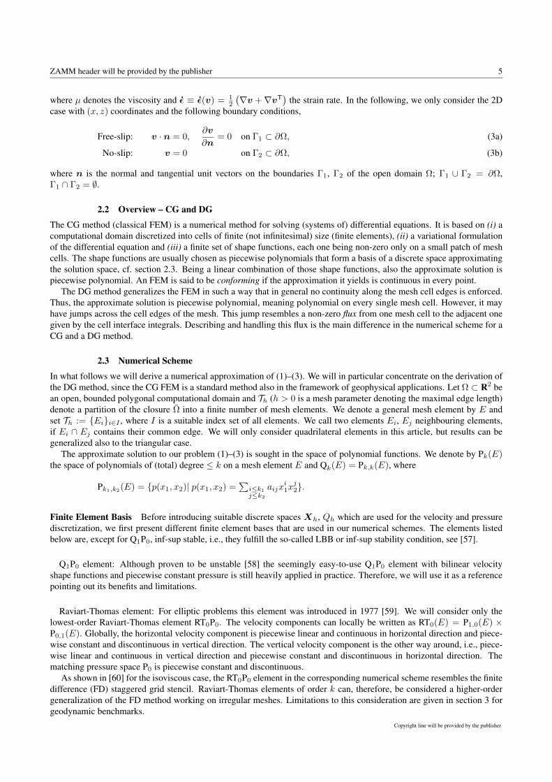
Finite Element Basis Before introducing suitable discrete spaces Xh, Qh which are used for the velocity and pressurediscretization, we first present different finite element bases that are used in our numerical schemes. The elements listedbelow are, except for Q1P0, inf-sup stable, i.e., they fulfill the so-called LBB or inf-sup stability condition, see [57].

Q1P0 element: Although proven to be unstable [58] the seemingly easy-to-use Q1P0 element with bilinear velocityshape functions and piecewise constant pressure is still heavily applied in practice. Therefore, we will use it as a referencepointing out its benefits and limitations.

Raviart-Thomas element: For elliptic problems this element was introduced in 1977 [59]. We will consider only thelowest-order Raviart-Thomas element RT0P0. The velocity components can locally be written as RT0(E) = P1,0(E) ×P0,1(E). Globally, the horizontal velocity component is piecewise linear and continuous in horizontal direction and piece-wise constant and discontinuous in vertical direction. The vertical velocity component is the other way around, i.e., piece-wise linear and continuous in vertical direction and piecewise constant and discontinuous in horizontal direction. Thematching pressure space P0 is piecewise constant and discontinuous.

As shown in [60] for the isoviscous case, the RT0P0 element in the corresponding numerical scheme resembles the finitedifference (FD) staggered grid stencil. Raviart-Thomas elements of order k can, therefore, be considered a higher-ordergeneralization of the FD method working on irregular meshes. Limitations to this consideration are given in section 3 forgeodynamic benchmarks.



Fig. 1 Degrees of freedom (DOFs) for the elements Q1P0, Q2P1, lowest-order Raviart-Thomas RT0P0 and Brezzi-Douglas-MariniBDM1P0 (left to right). Crosses and circles denote DOFs for horizontal and vertical velocity, respectively. Squares and arrows denotepressure and pressure gradient DOFs.

0

1

0

1

0

1

0

1

Fig. 2 Instances of basis functions for (horizontal) velocity component of the elements Q1P0, Q2P1, RT0P0, BDM1P0 (left to right).

Brezzi-Douglas-Marini element: This element was introduced in 1985 [61] following the Raviart-Thomas element inits approach to design a discrete basis of H0(div,Ω), cf. (4c), see also [62, §III.3]. Locally, it is bilinear like the Q1P0

element, BDM1(E) = Q1(E)2 with Q1(E) defined above. Across mesh edges, it is continuous in normal direction anddiscontinuous in tangential direction like the RT0P0 element. The matching pressure space is piecewise constant anddiscontinuous.

Q2P1 element: This element is based on a biquadratic approximation for velocity and a piecewise linear approximationfor pressure. On the same mesh this element reaches higher accuracy at increased computational cost compared to theQ1P0 element. As for the other elements the pressure approximation may encounter discontinuities across mesh edges.This element is commonly used for discretization of the Stokes flow.

In what follows we use the abbreviation Q1P0 or Q2P1 for the FEM based on using either the Q1P0 or the Q2P1 element,respectively. On the other hand we use the abbreviation RT0P0 or BDM1P0 for the DG method based on using either theRT0P0 or the BDM1P0 element, respectively.

Function Spaces The finite element bases Q1P0 and Q2P1 yield well-known continuous finite element methods, see,e.g., [63, III.§6]. In what follows we define suitable discrete spacesXh, Qh for the discretization of velocity and pressure,respectively, that will be used in the framework of the discontinuous Galerkin scheme.

Xh = u ∈ H0(div,Ω) : u|E ∈ RT0(E) or BDM1(E) ∀E, u · n = 0 on ∂Ω, (4a)

Qh = q ∈ L2(Ω) : q|E ∈ P0(E) ∀E,∫

Ωq = 0, (4b)

H0(div,Ω) = u ∈ (L2(Ω))2 : ∇ · u ∈ L2(Ω),u · n = 0 on ∂Ω. (4c)

Thus, the approximation for the velocity is div-conforming, i.e. included in H0(div,Ω). It has continuous normalcomponents across elements and will be globally divergence free in the space H0(div,Ω), cf. [60].

Scheme Derivation We now introduce notations for the jump and average of a (scalar or vector-valued) quantity u ∈ Rn,n ≥ 1, along an edge e = Ei ∩ Ej shared by two neighbouring mesh elements Ei, Ej with the respective outer normalvectors ni pointing to Ej , and nj pointing to Ei,

[u] ij := uj − ui, 〈u〉ij :=ui + uj

2, (5)



where ui denotes the limiting value of u from the mesh elements Ei along edge e. The analogous notation holds foruj . Fixing either of the normal vectors ni, nj as belonging to the edge e, we drop the index notation for the jump sinceni = −nj and thus [u] ijnj = [u] jini =: [u]ne. Consequently, we fix either of the normal vectors on interior edges andrefer to it as ne. For boundary edges e ⊂ ∂Ω the notation ne refers to the unique outward pointing normal. Secondly, wenote without proof the following Lemma, cf. e.g., [64],

Lemma 2.1 For a, b ∈ Rn, n ≥ 1, (or a ∈ R, b ∈ Rn, n > 1) the following equality applies:

[a · b] = 〈a〉 · [b] + [a] · 〈b〉 . (6)

Now, we will derive our DG approximation following [42], [65, 4.2 and 6.2], [66, 14.2]. Note that the different approachof [55] yields similar forms. First, multiplying the momentum conservation equation (1a) with a test function φ ∈ Xh

yields after elementwise integration by parts,∫E

2µ ε(φ) : ε(v)−∫∂E

φ · (τnE)−∫E

p(∇ · φ) +

∫∂E

pφ · nE =

∫E

−ρgz · φ, (7)

where nE denotes the unit outer normal of the mesh cell E and a : b the so-called Frobenius product, i.e., componentwiseinner product of two matrices. Let us look in more details at the second term summed with respect to the mesh cells:

−∑E∈Th

∫∂E

φ · (τnE) = −∑e∈Fh

∫e

[φ · τ ]ne −∑e⊂∂Ω

∫e

φ · τne. (8)

First, we would like to mention that the integrals along the boundary edges e ⊂ ∂Ω vanish due to the boundary conditions(3). Indeed, on Γ2 the test function vanishes due to the Dirichlet boundary conditions. On Γ1 we have

∑e⊂Γ1

∫eφµ(∇v+

(∇v)T)ne =∑e⊂Γ1

∫eφµ(∇v)Tne, since ∇v · ne = ∂v

∂ne= 0. Furthermore, we recall that Ω is a polygonal domain,

thus on each boundary segment we have a constant outer normal. Applying both conditions from (3a) we finally obtain that

(∇v)Tne =(∑2

j=1∂vj∂x1

ne,j ,∑2j=1

∂vj∂x2

ne,j

)T= 0 on Γ1.

Further, we exploit Lemma 2.1 and, as argued in [66], we apply the interior penalty method. Thus, we replace thenormal flux term, τn, by the discrete flux, 〈2µε(v)〉ne − σ

|e| [v], where σ is a suitable positive weight parameter, cf.also, e.g., [42, 4.6], [60]. In our numerical experiments presented in section 3 the parameter σ was chosen to be globallyconstant.

−∑e∈Fh

∫e

[φ · τ ]ne = −∑e∈Fh

∫e

[φ] · 〈τ 〉ne + 〈φ〉 · [τ ]ne (9)

= −∑e∈Fh

∫e

[φ] · τne (10)

' −∑e∈Fh

∫e

[φ] ·(〈2µε(v)〉ne −

σ

|e|[v]

). (11)

We have also used the fact that τne is continuous across mesh edges for v being the exact solution, cf. [67]. Further, µdenotes an average viscosity value depending on the values of µ on the mesh cells that adhere to the respective edge e. Wechoose µ to be the geometric average accommodating the fact that µ may change by orders of magnitude. We note that,for the chosen benchmark setups, this yields smaller errors than taking the arithmetic or harmonic mean. For other ways ofcomputing weighted averages in this context compare, e.g., [65, 4.5.2].

We note that the term [v] · 〈2µε(φ)〉 is zero for v being the exact solution. Therefore, we could add it to (or subtract itfrom) the previous term without losing consistency. These considerations yield the following bilinear form ah, which willbe used for the numerical scheme,

ah(v,φ) =∑E

∫E

2µε(φ) : ε(v) +∑e∈Fh

σ

|e|

∫e

[φ] · [v] (12a)

−∑e∈Fh

∫e

[φ] · 〈2µε(v)〉ne − ε∑e∈Fh

∫e

[v] · 〈2µε(φ)〉ne, v,φ ∈Xh. (12b)

For ε = 1,−1, 0, this is refered to as the symmetric, nonsymmetric or incomplete interior penalty Galerkin method(SIPG, NIPG, IIPG), respectively. SIPG methods have been introduced in [64], NIPG in [68], IIPG in [69]. We refer also



to other works, see, e.g., [52,70–73] and the references therein, where full numerical analysis of the discontinous Galerkinmethod with SIP for the Laplace equation is available. For more details on the differences of these methods, we refer thereader to [74, 1.2], [65, 5.3] and the references therein. Numerical results presented in this paper were obtained using theNIPG (ε = −1) that yielded best results for the considered benchmark problems.

The weak form of the incompressibility condition (1b) yields the bilinear form bh and is given by:

0 = bh(v, q) =∑E

∫E

(∇ · v)q, q ∈ Qh. (13)

To discretize the pressure terms from the momentum equation we extend the bilinear form bh, cf. [65, 6.1],

b∗h(φ, p) = −bh(φ, p) +∑e∈Fh

∫e

[p]φ · ne +∑e⊂∂Ω

∫e

pφ · ne, (14)

where we used that φ · ne is continuous across mesh edges. Note again that the boundary integrals vanish due to eq. (3).Now, we can state our DG approximation scheme: Find (v, p) ∈Xh ×Qh such that

ah(v,φ) + b∗h(φ, p) =

∫Ω

−ρgz · φ, ∀φ ∈Xh, (15a)

bh(v, q) = 0, ∀q ∈ Qh. (15b)

In [55] analytic properties of a large class of divergence-free DG methods have been investigated. The authors studieddiv-conforming spaces, which satisfy the condition ∇ · X(E) ⊆ P (E), where X(E) and P (E) are local spaces for theapproximation of velocity and pressure, respectively. Note that our local element RT0P0 satisfies the above condition. Theuse of the local space BDMk+1/Pk for velocity and pressure, respectively, have been analyzed in [75] in the frameworkof DG FEM. For a large class of DG methods (including our particular choice (15)) the stability and accuracy have beeninvestigated theoretically in [55]. In particular, it has been proven that the resulting methods satisfy the inf-sup stabilitycondition and that the following error estimates hold.

Let us denote by v, p, vh, ph the exact and approximate solutions (velocity vector and pressure), respectively. Moreoverlet v ∈ Hk+1(Ω), p ∈ Hk(Ω) is a regular solution and ‖·‖1,h is a suitable discrete H1 norm in the broken Sobolev spaceXh, i.e., ‖uh‖21,h =

∑E

∫E

(∇uh)2dx+∑e

∫eσh | [uh] |2 for any uh ∈Xh. Then it holds

‖v − vh‖1,h + ‖p− ph‖L2(Ω) ≤ chk (‖v‖k+1 + ‖p‖k) , (16)

where k ≥ 1, c > 0 is a constant independent of the mesh size h. Moreover, the approximate velocity vh is exactlydivergence-free and the resulting DG methods are conservative, energy-stable and optimally convergent, cf. [55] and [75].

Let us also point out that in [60] the author investigates the use of the RT0P0 element in the framework of divergence-freeDG methods. It has been proven that such a DG scheme is algebraically equivalent to the standard MAC finite differencescheme, that is often used in engineering applications in order to approximate the Stokes problem. Using this fact, we canapply the recent result of Li and Sun [76] who have proven superconvergence of the MAC scheme, i.e., the discrete L2

errors of pressure, velocity as well as gradient of velocity are of second order.In this paper we compare the behaviour of the above DG methods and standard, i.e. continuous finite elements, for some

typical geophysical tests. Recall that when we apply CG-FEM method the space Xh is a discrete space approximating(H1(Ω))2 with cellwise bilinear Q1 or cellwise biquadratic functions Q2. For the latter the pressure space Qh is the spaceof cellwise linear functions with mean value zero. Thus, we do not require that the discrete velocities for CG-FEM arediv-conforming (i.e., in H0(div,Ω)). Note that using the same bilinear forms without edge integrals the formulation abovecoincides with the standard variational formulation of incompressible Stokes flow in a CG-FEM setting, see, e.g., [63,III.§6], [66, 12.2].

2.4 Benchmark Setups

SolCx Benchmark The analytic solution to this benchmark was derived by Zhong [77] and our implementation fol-lows [22]. We include a Matlab function (SolCx.m) to compute the analytic solution in the online supplement to this articlethat is based on the one provided in Underworld [33]. The setup resembles a simplified mantle convection model with alateral viscosity jump caused by, e.g., a material interface. The flow is driven by a prescribed smooth density field.



free-slip

free-slip

1free-slip

free-slip

μ2μ1

ρ=sin(πz)cos(πx)

xz 1

free-slip

free-slip

1

μ2, ρ2

A

λ

0.1 μ1, ρ1

no-slip

no-slip

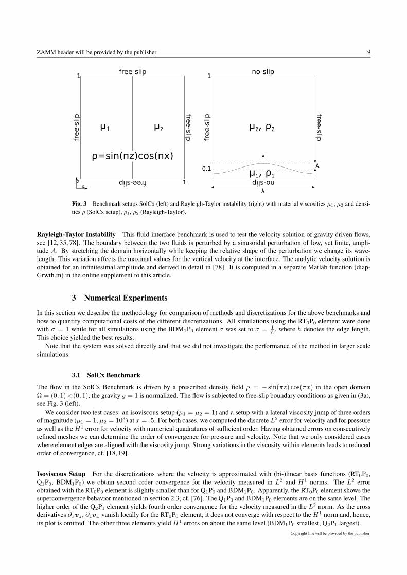
Fig. 3 Benchmark setups SolCx (left) and Rayleigh-Taylor instability (right) with material viscosities µ1, µ2 and densi-ties ρ (SolCx setup), ρ1, ρ2 (Rayleigh-Taylor).

Rayleigh-Taylor Instability This fluid-interface benchmark is used to test the velocity solution of gravity driven flows,see [12, 35, 78]. The boundary between the two fluids is perturbed by a sinusoidal perturbation of low, yet finite, ampli-tude A. By stretching the domain horizontally while keeping the relative shape of the perturbation we change its wave-length. This variation affects the maximal values for the vertical velocity at the interface. The analytic velocity solution isobtained for an infinitesimal amplitude and derived in detail in [78]. It is computed in a separate Matlab function (diap-Grwth.m) in the online supplement to this article.

3 Numerical Experiments

In this section we describe the methodology for comparison of methods and discretizations for the above benchmarks andhow to quantify computational costs of the different discretizations. All simulations using the RT0P0 element were donewith σ = 1 while for all simulations using the BDM1P0 element σ was set to σ = 1

h , where h denotes the edge length.This choice yielded the best results.

Note that the system was solved directly and that we did not investigate the performance of the method in larger scalesimulations.

3.1 SolCx Benchmark

The flow in the SolCx Benchmark is driven by a prescribed density field ρ = − sin(πz) cos(πx) in the open domainΩ = (0, 1)× (0, 1), the gravity g = 1 is normalized. The flow is subjected to free-slip boundary conditions as given in (3a),see Fig. 3 (left).

We consider two test cases: an isoviscous setup (µ1 = µ2 = 1) and a setup with a lateral viscosity jump of three ordersof magnitude (µ1 = 1, µ2 = 103) at x = .5. For both cases, we computed the discrete L2 error for velocity and for pressureas well as the H1 error for velocity with numerical quadratures of sufficient order. Having obtained errors on consecutivelyrefined meshes we can determine the order of convergence for pressure and velocity. Note that we only considered caseswhere element edges are aligned with the viscosity jump. Strong variations in the viscosity within elements leads to reducedorder of convergence, cf. [18, 19].

Isoviscous Setup For the discretizations where the velocity is approximated with (bi-)linear basis functions (RT0P0,Q1P0, BDM1P0) we obtain second order convergence for the velocity measured in L2 and H1 norms. The L2 errorobtained with the RT0P0 element is slightly smaller than for Q1P0 and BDM1P0. Apparently, the RT0P0 element shows thesuperconvergence behavior mentioned in section 2.3, cf. [76]. The Q1P0 and BDM1P0 elements are on the same level. Thehigher order of the Q2P1 element yields fourth order convergence for the velocity measured in the L2 norm. As the crossderivatives ∂xvz , ∂zvx vanish locally for the RT0P0 element, it does not converge with respect to the H1 norm and, hence,its plot is omitted. The other three elements yield H1 errors on about the same level (BDM1P0 smallest, Q2P1 largest).



Fig. 4 Analytic solution in SolCx benchmark as given by [77] for velocity (arrows) and pressure (color-coded). Left: Isoviscous setup,µ1 = µ2 = 1. Right: Viscosity jump of three orders of magnitude, µ1 = 1, µ2 = 103. The reference arrow lengths are 2.53 × 10−2

and 3.60 × 10−3, respectively, for the arrow originating at the point (x = 0, z = .5). Note that the pressure is discontinuous inthe variable viscosity setup and the jump is aligned with the viscosity jump. The analytic solution for the isoviscous setup is v =[− sin(πx) cos(πz); cos(πx) sin(πz)]/4π2, p = − cos(πx) cos(πz)/2π. The analytic solution of the variable-viscosity setup can befound in [77].

The L2 pressure error differs only slightly for the RT0P0 and the Q2P1 element as well as for the Q1P0 and the BDM1P0

element. For the latter ones it is at least two orders of magnitude smaller and has higher rate of convergence, which seemsto be influenced by superconvergence effects for this particular setup.

Let us consider the errors with respect to the number of degrees of freedom (DOFs) needed to reach a certain accuracy.The Q2P1 element still yields the smallest velocity error in the L2 norm. On the other hand, the Q1P0 element performsslightly better than the BDM1P0 element (and a lot better than the Q2P1 element) in terms of the H1 error in the velocityand the pressure error.

For the velocity and pressure error in the isoviscous SolCx setup see Figs. 5 and 6.

Lateral Viscosity Jump In this setup the velocity errors show a similar behavior as for the isoviscous case, i.e., theBDM1P0 and Q1P0 element converge with second order to the analytic solution with the error being at the same order ofmagnitude, while the Q2P1 element converges with fourth order and, therefore, reaches much higher accuracy at the sameresolution. For the BDM1P0 element the convergence order measured in the H1 norm is only 1.3, approximately, while thetwo conforming elements keep the order 2. The pressure errors for these three elements are of similar order and convergewith second order.

Considering the number of degrees of freedom the elements’ performance is similar to the isoviscous case. The Q2P1

element yields the best L2 error for the velocity while the Q1P0 element yields highest accuracy in terms of the H1 errorfor the velocity and L2 error for the pressure. For the velocity and pressure error in the SolCx setup with discontinuousviscosity see Figs. 7 and 8.

We omit the RT0P0 element for this setup as it does not converge to the analytic solution. Due to the simple structure ofthis element no coupling of the two velocity components can be captured in the numerical scheme given in section 2.3. Asthe cross derivatives ∂xvz , ∂zvx vanish element-wise, shear stress components are not taken into account in the discretescheme. Shear stress is zero in the isoviscous SolCx setup but non-zero for discontinuous viscosity. This explains why theRT0P0 element converges in the isoviscous case but not in the discontinuous viscosity case. We aim to further investigatethis problem in a future study.

We can deduce from Figs. 5 and 7 that the BDM1P0 element has about the same accuracy (in terms of the L2 errors)as the Q1P0 element for any fixed resolution. This is to be expected as both elements are of the same order, i.e. velocityis approximated with piecewise bilinear, pressure is approximated with piecewise constant shape functions. The RT0P0

element is computationally cheaper, yielding similar accuracy in simple setups like the isoviscous SolCx setup but fails forsetups with non-zero shear stress. The Q2P1 element, being of higher order, yields higher accuracy and higher order ofconvergence at the price of increased computational costs.



10−2

10−1

10−10

10−6

10−2 Slope: 2.0

Grid size

L 2error(v)

10−2

10−1

10−6

10−4

10−2

Slope: 2.0

Grid sizeH

1error(v)

10−2

10−1

10−10

10−6

10−2 Slope: 2.0

Grid size

L 2error(p)

Q1Q2RTBDM

Fig. 5 Isoviscous SolCx Benchmark: L2 (left) and H1 (center) errors for velocity and L2 error for pressure (right) for the four dis-cretizations Q1P0, Q2P1, RT0P0 and BDM1P0. The slope of the plots corresponds to the order of convergence towards the analyticsolution when increasing the mesh resolution, i.e., decreasing the grid size.

103

105

10−10

10−6

10−2

Slope: 1.0

#DOFs

L 2error(v)

103

105

10−6

10−4

10−2

Slope: 1.0

#DOFs

H1error(v)

103

105

10−10

10−6

10−2

Slope: 1.0

#DOFsL 2

error(p)

Q1Q2RTBDM

Fig. 6 Isoviscous SolCx Benchmark: L2 (left) and H1 (center) errors for velocity and L2 error for pressure (right) for the four dis-cretizations Q1P0, Q2P1, RT0P0 and BDM1P0. The slope of the plots corresponds to the order of convergence towards the analyticsolution when increasing the number of degrees of freedom.

10−2

10−1

10−10

10−6

10−2 Slope: 2.0

Slope: 4.0

Grid size

L 2error(v)

10−2

10−1

10−6

10−4

10−2

Slope: 1.28

Slope: 2.0

Grid size

H1error(v)

10−2

10−1

10−6

10−4

10−2

Slope: 2.0

Grid size

L 2error(p)

Q1Q2BDM

Fig. 7 Variable Viscosity SolCx Benchmark: L2 (left) and H1 (center) errors for velocity and L2 error for pressure (right) for the threediscretizations Q1P0, Q2P1 and BDM1P0. The slope of the plots corresponds to the order of convergence towards the analytic solutionwhen increasing the mesh resolution, i.e., decreasing the grid size.

103

105

10−10

10−6

10−2

Slope: 1.0

Slope: 2.0

#DOFs

L 2error(v)

103

105

10−6

10−4

10−2

Slope: 0.50

Slope: 1.0

#DOFs

H1error(v)

103

105

10−6

10−4

10−2

Slope: 1.0

#DOFs

L 2error(p)

Q1Q2BDM

Fig. 8 Variable Viscosity SolCx Benchmark: L2 (left) and H1 (center) errors for velocity and L2 error for pressure (right) for the threediscretizations Q1P0, Q2P1 and BDM1P0. The slope of the plots corresponds to the order of convergence towards the analytic solutionwhen increasing the number of degrees of freedom.



Table 1 Relative errors erel =∣∣∣K−Kan

Kan

∣∣∣ for the three elements at ϕ(λ∗exp) in the middle of the chosen range. Resolution

for all elements fixed at 50 by 50 elements.

erel(λ∗exp)

µ2/µ1 Q1P0 Q2P1 BDM1P0

103 4.9× 10−1 1.5× 10−3 5.0× 10−1

101 2.8× 10−1 1.4× 10−3 2.6× 10−1

100 6.0× 10−2 8.4× 10−4 1.0× 10−1

10−3 2.7× 10−1 3.6× 10−4 3.7× 10−1

While the Q1P0 and Q2P1 element keep the L2 order of convergence for the velocity when changing to the H1 norm,the convergence order of the BDM1P0 element decreases.

3.2 Rayleigh-Taylor Instability

In the Rayleigh-Taylor instability benchmark the flow is driven by the density difference ∆ρ = ρ2− ρ1 of the two materiallayers. Both, the density difference ∆ρ = 1 and the gravity g = 1 are normalized. The computational domain is setto be Ω = (0, λ) × (0, zmax), where zmax = 1, see Fig. 3 (right). The material interface follows a mesh edge with asinusoidal perturbation of amplitude A and wavelength λ, i.e., the elements adjacent to the perturbed edge are slightlydeformed. Hence, the mesh is not globally regular anymore. We vary the viscosity contrast 10−3 ≤ µ2/µ1 ≤ 103 andstudy the vertical velocity vz at the tip of the sinusoidal perturbation. The magnitude of this velocity also depends on thewavelength λ, i.e., for every viscosity contrast there is one dominant wavelength λ∗ that yields a maximal magnitude forthe vertical velocity in this location. We vary the wavelength λ in a certain range around the dominant wavelength λ∗exp thatwe determined experimentally, see the axis labels in Fig. 9 for the ranges of ϕ = 2π(zmax−zjump)/λ, zmax = 1, zjump = 0.1.

In this setup, the free-slip condition is imposed at the vertical boundaries, no-slip at the horizontal boundaries, see (3).We run two sets of experiments. Firstly, we fix the resolution to 50 by 50 elements. Secondly, we choose the resolution suchthat for all elements it yields approximately the same number of non-zero entries in the system matrix. In both cases wecompute the maximum vertical velocity vz for different wavelengths λ of the sinusoidal perturbation by changing the widthof the domain and we vary the viscosity contrasts between 10−3 and 103, fixing the perturbation amplitude at A = 10−4.A non-dimensional growth factor Kan = vz

A2µ2

∆ρ zjumpgcan be analytically derived as given in [78, sec. 6] and [12, sec. 16.2].

We compare the numerically retrieved value of K to the analytic one. For the same reasons as in the previous section weomit the RT0P0 element here.

We shall first consider the case µ2/µ1 ≤ 1, i.e., the top layer viscosity being less or equal to the bottom layer viscosity,with fixed resolution of 50 by 50 elements, see Fig. 9, bottom left. The Q2P1 element, as in all other cases, very accuratelyresembles the analytic value of the maximum vertical velocity while the Q1P0 and the BDM1P0 elements deviate stronger,see Tab. 1. Yet, the relative errors for the latter two stay in the same range.

For the same viscosity contrasts, but roughly equivalent memory usage of all three elements (Fig. 9, bottom right), theQ2P1 element is still the best choice. The relative error for the Q1P0 element is less than half of the error for the BDM1P0

element, see Tab. 2.In the case µ2/µ1 > 1, i.e. the top layer being more viscous than the bottom layer, the BDM1P0 element yields a

better approximation to the maximum vertical velocity than the Q1P0 element. Still, the Q2P1 element gives much higheraccuracy, see Fig. 9, top left, and Tab. 1. For equivalent memory usage (Fig. 9, top right, Tab. 2), this behavior changespartially. For some wavelengths at viscosity contrast µ2/µ1 = 103 the BDM1P0 element yields a smaller error, for othersthe Q1P0 element does. For µ2/µ1 = 101 the Q1P0 error, all in all, is smaller than the error obtained with the BDM1P0

element.Similar to the SolCx benchmark, using the Q2P1 element in the Rayleigh-Taylor instability benchmark, see Fig. 9, we

obtain very accurate approximations for any considered viscosity contrast. On the one hand, we can see the BDM1P0 andQ1P0 elements yielding an error of equal order of magnitude for the bottom layer viscosity being greater or equal to the toplayer viscosity (µ1 ≥ µ2). On the other hand, when the top layer viscosity exceeds the bottom layer viscosity, the BDM1P0

element yields better results than the Q1P0 element.

3.3 Computational Costs

Finally, we list the number of entries in the system matrix for the different discretizations as an indicator for computationalcosts of the solution and how much memory its assembly requires, see Tab. 3. It can be observed that the RT0P0 element is



φ

K

15 19 230

0.1

0.34

φ

K

15 19 230

0.1

0.34

AnalyticalQ1Q2BDM1

φ

K

11 15 190

0.1

0.25

φ

K

11 15 190

0.1

0.25

φ

K

6 9 120

0.01

0.08

φ

K6 9 12

00.01

0.08

φ

K [

×1

0–3

]

5/3 3 13/30

1

3.6

φ

K [

×1

0–3

]

5/3 3 13/30

1

3.6

Fig. 9 Rayleigh-Taylor Instability Benchmark: Non-dimensional growth factor K versus frequency ϕ = 2π(zmax − zjump)/λ, zmax = 1,zjump = .1. Solid lines give the analytically obtained value Kan at the tip of the sinusoidal perturbation (i.e., where vertical velocity ismaximal). Top to bottom: Viscosity contrasts µ2/µ1 = 103, 101, 100, 10−3. Left: Errors for Q1P0, Q2P1, BDM1P0 at fixed meshresolution of 50 by 50. Right: Errors for Q1P0(mesh resolution 90 by 90), Q2P1(40 by 40), BDM1P0 (60 by 60), i.e., such that thesystem matrix has approximately 4.5× 105 non-zero entries.

the cheapest one considered here. However, its drawbacks are obvious, as it fails to converge in relevant variable viscositybenchmark setups.

If one considers memory usage instead of mesh resolution one obtains different observations. For a fixed memory theQ1P0 element gives a higher accuracy than the BDM1P0 element that seemed to be competitive when fixing the meshresolution, cf. Figs. 6, 8.

In any case, regarding fixed memory limitations or fixed resolution, the Q2P1 element has best over-all performance.Copyright line will be provided by the publisher


Table 2 Relative errors erel =∣∣∣K−Kan

Kan

∣∣∣ for the three elements at ϕ(λ∗exp) in the middle of the chosen range. Resolution

for Q1P0, Q2P1, BDM1P0 element is 90 by 90, 40 by 40, 60 by 60 elements, respectively, yielding approximately thesame memory usage for all three elements (≈ 4.5× 105 non-zero entries in system matrix).

erel(λ∗exp)

µ2/µ1 Q1P0 Q2P1 BDM1P0

103 1.6× 10−1 2.4× 10−3 3.5× 10−1

101 9.7× 10−2 2.5× 10−3 1.8× 10−1

100 1.6× 10−2 1.6× 10−3 7.7× 10−2

10−3 9.0× 10−2 7.5× 10−4 2.6× 10−1

Table 3 Number of global degrees of freedom (DOFs) and of non-zero entries (NNZs) in the system matrix on a square32-by-32-mesh for the four discretizations. Note that the Q1P0 and Q2P1 elements are used in the standard finite elementframework while the RT0P0 and the BDM1P0 elements are used in the DG scheme derived in section 2.3.

Element DOFs NNZsRT0P0 3136 2.6× 104

Q1P0 3202 4.8× 104

BDM1P0 5248 1.2× 105

Q2P1 11 522 3.1× 105

4 Conclusions

The main aim of this paper was to study behaviour of the DG finite element method based on the use of div-conformingelements to approximate the Stokes flow with variable viscosity and examine how it compares in terms of accuracy andmemory usage to the standard CG finite element method for some typical geodynamic benchmark setups. In the DG schemewe employ the Raviart-Thomas (RT0P0) and the Brezzi-Douglas-Marini element (BDM1P0). In contrast to the Q1P0 finiteelement they fulfill the LBB stability condition, implying that they are more reliable.

We showed that the overall results are as accurate or more accurate than the ones obtained with the Q1P0 element in astandard finite element scheme considering a fixed mesh resolution. Yet, the Q1P0 CG method yields better results than theDG method using the BDM1P0 element when considering a fixed memory limitation. Secondly, being of first order bothof them are computationally less expensive than the Q2P1 element. However, whenever a second-order FEM like Q2P1 iscomputationally feasible, higher accuracy can be obtained compared to the DG method based on the BDM1P0 element orthe Q1P0 element in the classical FEM scheme.

The divergence-conforming property of the BDM1P0 and the RT0P0 element has been seen to be advantageous for, e.g.,Navier-Stokes equations [55] or Darcy flow [56]. However, in the tested benchmark setups this does not produce noticablebenefits. We would like to investigate this point in our future study on different test cases.

The BDM1P0 element yields good results in all tested setups and offers an alternative to the LBB-unstable Q1P0 element.The setups presented in this article do not lead to common instabilities of the Q1P0 element. However, we want to pointout that for the Stokes flow the reliability of the BDM1P0 element is its major advantage when being compared to the Q1P0

element. This could well be taken as justification to deploy this discretization.Due to the flexibility of hp-refinement within the DG methods, it is possible to apply low order discretizations in the

vicinity of viscosity jumps, but higher order polynomials in the areas with constant or smoothly varying viscosity. Thismight be a promising future direction for complex geodynamic simulations.

Acknowledgements This work has been funded and supported by the Computational Sciences Center and by the Max Planck GraduateCenter with the Johannes Gutenberg-Universitat Mainz (MPGC).

The deployed Matlab code is provided as an electronic supplement with the article web resource.

References

[1] P. A. Allen and J. R. Allen, Basin Analysis: Principles and Applications (Wiley, 2005).[2] C. J. Warren, C. Beaumont, and R. A. Jamieson, Modelling tectonic styles and ultra-high pressure (UHP) rock exhumation during

the transition from oceanic subduction to continental collision, Earth Planet. Sc. Lett. 267(1–2), 129–145 (2008).[3] B. J. P. Kaus, C. Steedman, and T. W. Becker, From passive continental margin to mountain belt: Insights from analytical and

numerical models and application to Taiwan, Phys. Earth Planet. Inter. 171(1–4), 235–251 (2008).



[4] S. M. Lechmann, S. M. Schmalholz, G. Hetenyi, D. A. May, and B. J. P. Kaus, Quantifying the impact of mechanical layering andunderthrusting on the dynamics of the modern India-Asia collisional system with 3-D numerical models, J. Geophys. Res. 119(1),616–644 (2014).

[5] L. Moresi, P. G. Betts, M. S. Miller, and R. A. Cayley, Dynamics of continental accretion, Nature(Advance online publication)(2014).

[6] F. Crameri, H. Schmeling, G. J. Golabek, T. Duretz, R. Orendt, S. J. H. Buiter, D. A. May, B. J. P. Kaus, T. V. Gerya, and P. J.Tackley, A comparison of numerical surface topography calculations in geodynamic modelling: An evaluation of the ‘sticky air’method, Geophys. J. Int. 189(1), 38–54 (2012).

[7] G. Schubert, D. L. Turcotte, and P. Olson, Mantle Convection in the Earth and Planets (Cambridge University Press, 2001).[8] Y. Deubelbeiss, B. J. P. Kaus, J. A. D. Connolly, and L. Caricchi, Potential causes for the non-Newtonian rheology of crystal-

bearing magmas, Geochem. Geophy. Geosy. 12(5) (2011).[9] T. Keller, D. A. May, and B. J. P. Kaus, Numerical modelling of magma dynamics coupled to tectonic deformation of lithosphere

and crust, Geophys. J. Int. 195(3), 1406–1442 (2013).[10] T. E. Johnson, M. Brown, B. J. P. Kaus, and J. A. van Tongeren, Delamination and recycling of Archaean crust caused by gravita-

tional instabilities, Nature Geosci. 7(1), 47–52 (2014).[11] D. L. Turcotte and G. Schubert, Geodynamics (Cambridge University Press, 2002).[12] T. V. Gerya, Introduction to Numerical Geodynamic Modelling (Cambridge University Press, 2010).[13] A. Ismail-Zadeh and P. Tackley, Computational Methods for Geodynamics (Cambridge University Press, 2010).[14] T. W. Becker and B. J. P. Kaus, Numerical Geodynamics – An introduction to computational methods with focus on solid Earth

applications of continuum mechanics, http://geodynamics.usc.edu/%7Ebecker/preprints/Geodynamics540.pdf (Lecture Notes),2010.

[15] B. J. P. Kaus, H. Muhlhaus, and D. A. May, A stabilization algorithm for geodynamic numerical simulations with a free surface,Physics of the Earth and Planetary Interiors 181(1–2), 12–20 (2010).

[16] P. J. Tackley, Modelling compressible mantle convection with large viscosity contrasts in a three-dimensional spherical shell usingthe yin-yang grid, Phys. Earth Planet. Inter. 171(1–4), 7–18 (2008).

[17] M. Thielmann and B. J. P. Kaus, Shear heating induced lithospheric-scale localization: Does it result in subduction?, Earth Planet.Sc. Lett. 359–360, 1–13 (2012).

[18] Y. Deubelbeiss and B. J. P. Kaus, Comparison of Eulerian and Lagrangian numerical techniques for the Stokes equations in thepresence of strongly varying viscosity, Phys. Earth Planet. Inter. 171(1–4), 92–111 (2008).

[19] M. Thielmann, D. May, and B. Kaus, Discretization errors in the hybrid finite element particle-in-cell method, Pure Appl. Geo-phys. 171(9), 2165–2184 (2014).

[20] P. J. Tackley, Effects of strongly temperature-dependent viscosity on time-dependent, three-dimensional models of mantle con-vection, Geophys. Res. Lett. 20(20), 2187–2190 (1993).

[21] T. V. Gerya and D. A. Yuen, Characteristics-based marker-in-cell method with conservative finite-differences schemes for model-ing geological flows with strongly variable transport properties, Phys. Earth Planet. Inter. 140(4), 293–318 (2003).

[22] D. A. May and L. Moresi, Preconditioned Iterative Methods for Stokes Flow Problems Arising in Computational Geodynamics,Phys. Earth Planet. Inter. 171(1–4), 33–47 (2008).

[23] T. Duretz, D. A. May, T. V. Gerya, and P. J. Tackley, Discretization errors and free surface stabilization in the finite difference andmarker-in-cell method for applied geodynamics: A numerical study, Geochem. Geophy. Geosy. 12(7), 1200–1225 (2011).

[24] C. Huttig and K. Stemmer, Finite volume discretization for dynamic viscosities on Voronoi grids, Phys. Earth Planet. Inter.171(1–4), 137–146 (2008).

[25] S. A. Melchior, V. Legat, P. v. Dooren, and A. J. Wathen, Analysis of preconditioned iterative solvers for incompressible flowproblems, Int. J. Numer. Meth. Fluids 68(3), 269–286 (2012).

[26] M. Benzi, G. H. Golub, and J. Liesen, Numerical solution of saddle point problems, Acta numerica 14, 1–137 (2005).[27] C. Burstedde, O. Ghattas, M. Gurnis, G. Stadler, E. Tan, T. Tu, L. C. Wilcox, and S. Zhong, Scalable adaptive mantle convection

simulation on petascale supercomputers, in: Proceedings of the 2008 ACM/IEEE Conference on Supercomputing, , SC ’08 (IEEEPress, Piscataway, NJ, USA, 2008), pp. 62:1–62:15.

[28] C. Burstedde, G. Stadler, L. Alisic, L. C. Wilcox, E. Tan, M. Gurnis, and O. Ghattas, Large-scale adaptive mantle convectionsimulation, Geophys. J. Int. 192(3), 889–906 (2013).

[29] M. Furuichi, D. A. May, and P. J. Tackley, Development of a Stokes flow solver robust to large viscosity jumps using a Schurcomplement approach with mixed precision arithmetic, J. Comput. Phys. 230(24), 8835–8851 (2011).

[30] B. E. Griffith, An accurate and efficient method for the incompressible Navier-Stokes equations using the projection method as apreconditioner, J. Comput. Phys. 228(20), 7565–7595 (2009).

[31] M. Cai, A. J. Nonaka, J. B. Bell, B. E. Griffith, and A. Donev, Efficient Variable-Coefficient Finite-Volume Stokes Solvers, arXivpreprint arXiv:1308.4605v2 (2013).

[32] S. Zhong, Constraints on thermochemical convection of the mantle from plume heat flux, plume excess temperature, and uppermantle temperature, J. Geophys. Res. 111(B4) (2006).

[33] L. Moresi, S. Quenette, V. Lemiale, C. Meriaux, B. Appelbe, and H. B. Muhlhaus, Computational approaches to studying non-linear dynamics of the crust and mantle, Phys. Earth Planet. Inter. 163(1–4), 69–82 (2007).

[34] M. Dabrowski, M. Krotkiewski, and D. W. Schmid, MILAMIN: MATLAB-based finite element method solver for large problems,Geochem. Geophy. Geosy. 9(4) (2008).

[35] A. A. Popov and S. V. Sobolev, SLIM3D: A Tool for Three-dimensional Thermomechanical Modeling of Lithospheric Deforma-tion with Elasto-visco-plastic Rheology, Phys. Earth Planet. Inter. 171(1–4), 55–75 (2008).



[36] Y. Mishin, Adaptive multiresolution methods for problems of computational geodynamics, PhD thesis, ETH Zurich, 2011.[37] D. A. May, J. Brown, and L. Le Pourhiet, ptatin3d: High-performance methods for long-term lithospheric dynamics, 2014.[38] L. C. Wilcox, G. Stadler, C. Burstedde, and O. Ghattas, A high-order discontinuous Galerkin method for wave propagation

through coupled elastic-acoustic media, J. Comput. Phys. 229(24), 9373–9396 (2010).[39] C. R. Dohrmann and P. B. Bochev, A stabilized finite element method for the Stokes problem based on polynomial pressure

projections, Int. J. Numer. Meth. Fluids 46(2), 183–201 (2004).[40] P. Bochev, C. Dohrmann, and M. Gunzburger, Stabilization of Low-order Mixed Finite Elements for the Stokes Equations, SIAM

J. Numer. Anal. 44(1), 82–101 (2006).[41] C. Burstedde, O. Ghattas, G. Stadler, T. Tu, and L. C. Wilcox, Parallel scalable adjoint-based adaptive solution of variable-

viscosity Stokes flow problems, Comput. Method. Appl. M. 198(21–26), 1691–1700 (2009).[42] M. Feistauer, J. Felcman, and I. Straskraba, Mathematical and Computational Methods for Compressible Flow (Oxford University

Press, 2003).[43] B. Cockburn and C. Shu, The Local Discontinuous Galerkin Method for Time-Dependent Convection-Diffusion Systems, SIAM

J. Numer. Anal. 35(6), 2440–2463 (1998).[44] M. J. Guillot, B. Riviere, and M. F. Wheeler, Discontinuous Galerkin methods for mass conservation equations for environmental

modelling, Dev. Water Sci. 47, 939–946 (2002).[45] M. Feistauer and V. Kucera, On a Robust Discontinuous Galerkin Technique for the Solution of Compressible Flow, J. Comput.

Phys. 224(1), 208–221 (2007).[46] J. Aarnes and B. O. Heimsung, Multiscale Discontinuous Galerkin Methods for Elliptic Problems with Multiple Scales, in: Mul-

tiscale Methods in Science and Engineering, edited by B. Engquist, P. Lotstedt, and O. Runborg, Lecture Notes in ComputationalScience and Engineering Vol. 44 (Springer, 2005), pp. 1–20.

[47] N. K. Burgess and D. J. Mavriplis, hp-Adaptive Discontinuous Galerkin Solver for the Navier-Stokes Equations, AIAA J. 50(12),2682–2694 (2012).

[48] S. Giani, High-order/hp-adaptive discontinuous Galerkin finite element methods for acoustic problems, Computing 95(1), 215–234 (2013).

[49] A. Baggag, H. Atkins, and D. Keyes, Parallel Implementation of the Discontinuous Galerkin Method, Tech. rep., Institute forComputer Applications in Science and Engineering (ICASE), 1999.

[50] H. Luo, L. Luo, A. Ali, R. Nourgaliev, and C. Cai, A Parallel, Reconstructed Discontinuous Galerkin Method for the CompressibleFlows on Arbitrary Grids, Commun. Comput. Phys. 9(2), 363–389 (2011).

[51] B. Cockburn, G. E. Karniadakis, and C. W. Shu (eds.), Discontinuous Galerkin Methods: Theory, Computation, and Applications,Lecture Notes in Computational Science and Engineering, Vol. 11 (Springer, 2000).

[52] D. N. Arnold, F. Brezzi, B. Cockburn, and L. D. Marini, Unified Analysis of Discontinuous Galerkin Methods for Elliptic Prob-lems, SIAM J. Numer. Anal. 39(5), 1749–1779 (2002).

[53] V. Etienne, E. Chaljub, J. Virieux, and N. Glinsky, An hp-adaptive discontinuous Galerkin finite-element method for 3-D elasticwave modelling, Geophys. J. Int. 183(2), 941–962 (2010).

[54] D. Pageot, S. Operto, M. Vallee, R. Brossier, and J. Virieux, A parametric analysis of two-dimensional elastic full waveforminversion of teleseismic data for lithospheric imaging, Geophys. J. Int. 193(3), 1479–1505 (2013).

[55] B. Cockburn, G. Kanschat, and D. Schotzau, A Note on Discontinuous Galerkin Divergence-free Solutions of the Navier-StokesEquations, J. Sci. Comput. 31(1–2), 61–73 (2007).

[56] V. J. Ervin, Computational bases for RTk and BDMk on triangles, Comput. Math. Appl. 64(8), 2765–2774 (2012).[57] Z. Cai and S. Zhang, Mixed methods for stationary Navier-Stokes equations based on pseudostress-pressure-velocity formulation,

Math. Comput. 81(280), 1903–1927 (2012).[58] D. Griffiths and D. Silvester, Unstable modes of the Q1-P0 element, MIMS EPrint 2011.44, Manchester Institute for Mathematical

Sciences, University of Manchester, Manchester, UK, 2011, This item originally appeared as MCCM Report 257 in 1994.[59] P. Raviart and J. Thomas, A Mixed Finite Element Method for 2-nd Order Elliptic Problems, in: Mathematical Aspects of Finite

Element Methods, edited by I. Galligani and E. Magenes, Lecture Notes in Mathematics Vol. 606 (Springer, 1977), chap. 19,pp. 292–315.

[60] G. Kanschat, Divergence-free Discontinuous Galerkin Schemes for the Stokes Equations and the MAC Scheme, Int. J. Numer.Meth. Fluids 56(7), 941–950 (2008).

[61] F. Brezzi, J. Douglas, Jr., and L. D. Marini, Two Families of Mixed Finite Elements for Second Order Elliptic Problems, Numer.Math. 47(2), 217–235 (1985).

[62] F. Brezzi and M. Fortin, Mixed and Hybrid Finite Element Methods (Springer, New York, NY, USA, 1991).[63] D. Braess, Finite elements: Theory, fast solvers, and applications in solid mechanics, 3rd edition (Cambridge University Press,

2007).[64] M. F. Wheeler, An Elliptic Collocation-Finite Element Method with Interior Penalties, SIAM J. Numer. Anal. 15(1), 152–161

(1978).[65] D. A. Di Pietro and A. Ern, Mathematical Aspects of Discontinuous Galerkin Methods, Mathematiques et Applications, Vol. 69

(Springer, Berlin, 2012).[66] M. Larson and F. Bengzon, The Finite Element Method: Theory, Implementation and Applications (Springer, 2013).[67] J. Necas, Direct Methods in the Theory of Elliptic Equations (Springer, 2012).[68] J. T. Oden, I. Babuska, and C. E. Baumann, A Discontinuous hp Finite Element Method for Diffusion Problems, J. Comput. Phys.

146(2), 491–519 (1998).



[69] C. Dawson, S. Sun, and M. F. Wheeler, Compatible algorithms for coupled flow and transport, Comput. Method. Appl. M.193(23–26), 2565–2580 (2004).

[70] D. N. Arnold, An interior penalty finite element method with discontinuous elements, SIAM J. Numer. Anal. 19(4), 742–760(1982).

[71] B. Riviere, M. F. Wheeler, and V. Girault, Improved energy estimates for interior penalty, constrained and discontinuous Galerkinmethods for elliptic problems. Part I, Comput. Geosci. 3(3-4), 337–360 (1999).

[72] F. Brezzi, G. Manzini, D. Marini, P. Pietra, and A. Russo, Discontinuous Galerkin approximations for elliptic problems, Numer.Meth. Part. D. E. 16(4), 365–378 (2000).

[73] Z. Chen and H. Chen, Pointwise Error Estimates of Discontinuous Galerkin Methods with Penalty for Second-Order EllipticProblems, SIAM J. Numer. Anal. 42(3), 1146–1166 (2004).

[74] B. Riviere, Discontinuous Galerkin Methods For Solving Elliptic And Parabolic Equations: Theory and Implementation (Societyfor Industrial and Applied Mathematics, Philadelphia, PA, USA, 2008).

[75] B. Cockburn, G. Kanschat, and D. Schotzau, A locally conservative LDG method for the incompressible Navier-Stokes equations,Math. Comput. 74(251), 1067–1095 (2005).

[76] J. Li and S. Sun, The Superconvergence Phenomenon and Proof of the MAC Scheme for the Stokes Equations on Non-uniformRectangular Meshes, J. Sci. Comput. pp. 1–22 (2014).

[77] S. Zhong, Analytic Solutions for Stokes’ Flow with Lateral Variations in Viscosity, Geophys. J. Int. 124(1), 18–28 (1996).[78] H. Ramberg, Instability of Layered Systems in the Field of Gravity, Phys. Earth Planet. Inter. 1(7), 427–447 (1968).


Comparison of Continuous and Discontinuous Galerkin Approaches ...

Documents

Transcript of Comparison of Continuous and Discontinuous Galerkin Approaches ...