EXPERIMENTAL COMPARISON OF DISCRIMINATIVE LEARNING APPROACHES...
100
EXPERIMENTAL COMPARISON OF DISCRIMINATIVE LEARNING APPROACHES FOR CHINESE WORD SEGMENTATION by Dong Song B.Sc., Simon Fraser University, 2005 a thesis submitted in partial fulfillment of the requirements for the degree of Master of Science in the School of Computing Science c Dong Song 2008 SIMON FRASER UNIVERSITY Summer 2008 All rights reserved. This work may not be reproduced in whole or in part, by photocopy or other means, without the permission of the author.
Transcript of EXPERIMENTAL COMPARISON OF DISCRIMINATIVE LEARNING APPROACHES...
EXPERIMENTAL COMPARISON OF DISCRIMINATIVE
LEARNING APPROACHES
FOR CHINESE WORD SEGMENTATION
by
Dong Song
B.Sc., Simon Fraser University, 2005
a thesis submitted in partial fulfillment
of the requirements for the degree of
Master of Science
in the School
of
Computing Science
c© Dong Song 2008
SIMON FRASER UNIVERSITY
Summer 2008
All rights reserved. This work may not be
reproduced in whole or in part, by photocopy
or other means, without the permission of the author.

APPROVAL
Name: Dong Song
Degree: Master of Science
Title of thesis: Experimental Comparison of Discriminative Learning Approaches
for Chinese Word Segmentation
Examining Committee: Dr. Ke Wang
Chair
Dr. Anoop Sarkar, Senior Supervisor
Dr. Fred Popowich, Supervisor
Dr. Ping Xue, External Examiner
Date Approved:
ii

Abstract
Natural language processing tasks assume that the input is tokenized into individual words.
In languages like Chinese, however, such tokens are not available in the written form. This
thesis explores the use of machine learning to segment Chinese sentences into word tokens.
We conduct a detailed experimental comparison between various methods for word seg-
mentation. We have built two Chinese word segmentation systems and evaluated them on
standard data sets.
The state of the art in this area involves the use of character-level features where the
best segmentation is found using conditional random fields (CRF). The first system we
implemented uses a majority voting approach among different CRF models and dictionary-
based matching, and it outperforms the individual methods. The second system uses novel
global features for word segmentation. Feature weights are trained using the averaged
perceptron algorithm. By adding global features, performance is significantly improved
compared to character-level CRF models.
Key words: word segmentation; machine learning; natural language processing.
iii

To my homeland
iv

Acknowledgments
I would like to express my sincere gratitude and respect to my senior supervisor, Dr. Anoop
Sarkar. His immense knowledge in natural language processing, his enthusiasm, support,
and patience, taken together, make him an excellent mentor and advisor.
I would also like to thank my supervisor, Dr. Fred Popowich, and my thesis examiner,
Dr. Ping Xue, for their great help towards my thesis. Also, I thank all members in the
natural language lab at Simon Fraser University and all my other friends for their continuous
support, and I thank Adam Lein for proofreading my thesis.
The most important, I am grateful to my parents for their endless love, encouragement
and support.
v

Contents
Approval ii
Abstract iii
Dedication iv
Acknowledgments v
Contents vi
List of Tables ix
List of Figures xi
1 Introduction 1
1.1 Challenges of Chinese Word Segmentation . . . . . . . . . . . . . . . . . . . . 1
1.2 Motivation to Study This Problem . . . . . . . . . . . . . . . . . . . . . . . . 2
1.3 Introduction to SIGHAN Bakeoff . . . . . . . . . . . . . . . . . . . . . . . . . 4
1.4 Approaches and Contributions . . . . . . . . . . . . . . . . . . . . . . . . . . 5
1.5 Thesis Outline . . . . . . . . . . . . . . . . . . . . . . . . . . . . . . . . . . . 6
2 General Approaches 7
2.1 Dictionary-based Matching . . . . . . . . . . . . . . . . . . . . . . . . . . . . 8
2.1.1 Greedy longest matching algorithm . . . . . . . . . . . . . . . . . . . . 8
2.1.2 Segmentation using unigram word frequencies . . . . . . . . . . . . . . 9
2.2 Sequence Learning Algorithms . . . . . . . . . . . . . . . . . . . . . . . . . . 11
2.2.1 HMM - A Generative Model . . . . . . . . . . . . . . . . . . . . . . . 12
vi

2.2.2 CRF - A Discriminative Model . . . . . . . . . . . . . . . . . . . . . . 18
2.3 Global Linear Models . . . . . . . . . . . . . . . . . . . . . . . . . . . . . . . 21
2.3.1 Perceptron Learning Approach . . . . . . . . . . . . . . . . . . . . . . 22
2.3.2 Exponentiated Gradient Approach . . . . . . . . . . . . . . . . . . . . 26
2.4 Summary . . . . . . . . . . . . . . . . . . . . . . . . . . . . . . . . . . . . . . 30
3 Majority Voting Approach 31
3.1 Overall System Description . . . . . . . . . . . . . . . . . . . . . . . . . . . . 31
3.2 Greedy Longest Matching . . . . . . . . . . . . . . . . . . . . . . . . . . . . . 33
3.3 CRF Model with Maximum Subword-based Tagging . . . . . . . . . . . . . . 33
3.4 CRF Model with Minimum Subword-based Tagging . . . . . . . . . . . . . . 34
3.5 Character-level Majority Voting . . . . . . . . . . . . . . . . . . . . . . . . . . 37
3.5.1 The Voting Procedure . . . . . . . . . . . . . . . . . . . . . . . . . . . 37
3.6 Post-processing Step . . . . . . . . . . . . . . . . . . . . . . . . . . . . . . . . 37
3.7 Experiments and Analysis . . . . . . . . . . . . . . . . . . . . . . . . . . . . . 39
3.7.1 Experiment Corpora Statistics . . . . . . . . . . . . . . . . . . . . . . 39
3.7.2 Results on the Experiment Corpora . . . . . . . . . . . . . . . . . . . 39
3.7.3 Error analysis . . . . . . . . . . . . . . . . . . . . . . . . . . . . . . . . 44
3.8 Minimum Subword-based CRF versus Character-based CRF . . . . . . . . . . 45
3.8.1 Experiments . . . . . . . . . . . . . . . . . . . . . . . . . . . . . . . . 45
3.8.2 Significance Test . . . . . . . . . . . . . . . . . . . . . . . . . . . . . . 49
3.9 Summary of the Chapter . . . . . . . . . . . . . . . . . . . . . . . . . . . . . . 50
4 Global Features and Global Linear Models 52
4.1 Averaged Perceptron Global Linear Model . . . . . . . . . . . . . . . . . . . . 53
4.2 Detailed System Description . . . . . . . . . . . . . . . . . . . . . . . . . . . . 54
4.2.1 N-best Candidate List . . . . . . . . . . . . . . . . . . . . . . . . . . . 54
4.2.2 Feature Templates . . . . . . . . . . . . . . . . . . . . . . . . . . . . . 55
4.2.3 A Perceptron Learning Example with N-best Candidate List . . . . . 57
4.3 Experiments . . . . . . . . . . . . . . . . . . . . . . . . . . . . . . . . . . . . . 60
4.3.1 Parameter Pruning . . . . . . . . . . . . . . . . . . . . . . . . . . . . . 60
4.3.2 Experiment Results . . . . . . . . . . . . . . . . . . . . . . . . . . . . 63
4.3.3 Significance Test . . . . . . . . . . . . . . . . . . . . . . . . . . . . . . 63
4.3.4 Error Analysis . . . . . . . . . . . . . . . . . . . . . . . . . . . . . . . 67
vii

4.4 Global Feature Weight Learning . . . . . . . . . . . . . . . . . . . . . . . . . 67
4.5 Comparison to Beam Search Decoding . . . . . . . . . . . . . . . . . . . . . . 69
4.5.1 Beam search decoding . . . . . . . . . . . . . . . . . . . . . . . . . . . 69
4.5.2 Experiments . . . . . . . . . . . . . . . . . . . . . . . . . . . . . . . . 69
4.6 Exponentiated Gradient Algorithm . . . . . . . . . . . . . . . . . . . . . . . . 75
4.7 Related Work . . . . . . . . . . . . . . . . . . . . . . . . . . . . . . . . . . . . 78
4.8 Summary of the Chapter . . . . . . . . . . . . . . . . . . . . . . . . . . . . . . 79
5 Conclusion 80
5.1 Thesis Summary . . . . . . . . . . . . . . . . . . . . . . . . . . . . . . . . . . 80
5.2 Contribution . . . . . . . . . . . . . . . . . . . . . . . . . . . . . . . . . . . . 81
5.3 Future Research . . . . . . . . . . . . . . . . . . . . . . . . . . . . . . . . . . 81
Bibliography 83
viii

List of Tables
2.1 An example for segmentation using unigram word frequencies . . . . . . . . . 10
2.2 Transition matrix . . . . . . . . . . . . . . . . . . . . . . . . . . . . . . . . . . 15
2.3 Emission matrix . . . . . . . . . . . . . . . . . . . . . . . . . . . . . . . . . . 15
2.4 Example for updating dual variables and the weight parameter vector in EG 29
3.1 CRF feature template . . . . . . . . . . . . . . . . . . . . . . . . . . . . . . . 35
3.2 An example for the character-level majority voting . . . . . . . . . . . . . . . 37
3.3 Performance (in percentage) on the MSRA held-out set . . . . . . . . . . . . 38
3.4 Performance (in percentage) after post-processing on the MSRA heldout set . 39
3.5 Statistics for the CityU, MSRA and UPUC training corpora . . . . . . . . . . 39
3.6 Number of sentences for the CityU, MSRA and UPUC test sets . . . . . . . . 40
3.7 Performance (in percentage) on the CityU corpus . . . . . . . . . . . . . . . . 40
3.8 Performance (in percentage) on the MSRA corpus . . . . . . . . . . . . . . . 40
3.9 Performance (in percentage) on the UPUC corpus . . . . . . . . . . . . . . . 42
3.10 Performance (in percentage) on the MSRA corpus, substituting the greedy
longest matching method with the unigram word frequency-based method in
majority voting . . . . . . . . . . . . . . . . . . . . . . . . . . . . . . . . . . . 43
3.11 Performance (in percentage) for majority voting using character-based CRF
algorithm on MSRA held-out set . . . . . . . . . . . . . . . . . . . . . . . . . 45
3.12 Performance (in percentage) on the CityU corpus, voting using the character-
based CRF algorithm . . . . . . . . . . . . . . . . . . . . . . . . . . . . . . . 46
3.13 Performance (in percentage) on the MSRA corpus, voting using the character-
based CRF algorithm . . . . . . . . . . . . . . . . . . . . . . . . . . . . . . . 46
3.14 Performance (in percentage) on the UPUC corpus, voting using the character-
based CRF algorithm . . . . . . . . . . . . . . . . . . . . . . . . . . . . . . . 48
ix
3.15 Word error distribution on the CityU corpus, from majority voting methods . 49
3.16 Word error distribution on the MSRA corpus, from majority voting methods 49
3.17 Word error distribution on the UPUC corpus, from majority voting methods 49
3.18 P-values computed using the McNemar’s test on the CityU, MSRA and
UPUC corpora, for comparison of majority voting methods . . . . . . . . . . 50
4.1 Local feature templates . . . . . . . . . . . . . . . . . . . . . . . . . . . . . . 56
4.2 Global feature templates . . . . . . . . . . . . . . . . . . . . . . . . . . . . . . 56
4.3 Updated weight vector w1 in the perceptron learning example . . . . . . . . . 58
4.4 Updated weight vector w2 in the perceptron learning example . . . . . . . . . 59
4.5 Final weight vector in the perceptron learning example . . . . . . . . . . . . . 60
4.6 Performance (in percentage) on CityU, MSRA, and UPUC Corpora . . . . . 64
4.7 Word error distribution on the CityU corpus . . . . . . . . . . . . . . . . . . 65
4.8 Word error distribution on the MSRA corpus . . . . . . . . . . . . . . . . . . 66
4.9 Word error distribution on the UPUC corpus . . . . . . . . . . . . . . . . . . 66
4.10 P-values computed using the McNemar’s test on the CityU, MSRA and
UPUC corpora, for comparison between the averaged perceptron using global
features and the character-based CRF . . . . . . . . . . . . . . . . . . . . . . 66
4.11 F-scores (in percentage) obtained by using various ways to transform global
feature weights and by updating their weights in averaged perceptron learn-
ing. The experiments are done on the UPUC and CityU corpora. . . . . . . . 68
4.12 F-scores (in percentage) with different training set sizes for the averaged
perceptron learning with beam search decoding . . . . . . . . . . . . . . . . . 71
4.13 Performance (in percentage) Comparison between the averaged perceptron
training using beam search decoding method and that using re-ranking method 73
4.14 The ratio from examining how many sentences in the gold standard also
appear within the 20-best candidate list, for the CityU, MSRA, UPUC, and
PU test sets . . . . . . . . . . . . . . . . . . . . . . . . . . . . . . . . . . . . . 74
4.15 Performance (in percentage) from the EG algorithms, comparing with those
from the perceptron learning methods and the character-based CRF method 77
x

List of Figures
2.1 Graph with different paths for segmentation using unigram word frequencies . 10
2.2 An HMM example . . . . . . . . . . . . . . . . . . . . . . . . . . . . . . . . . 13
2.3 The Viterbi algorithm . . . . . . . . . . . . . . . . . . . . . . . . . . . . . . . 14
2.4 Step 1 of the Viterbi algorithm for the example . . . . . . . . . . . . . . . . . 16
2.5 Step 2 of the Viterbi algorithm for the example . . . . . . . . . . . . . . . . . 16
2.6 Step 3.2 of the Viterbi algorithm for the example . . . . . . . . . . . . . . . . 17
2.7 Back Traversing Step of the Viterbi algorithm for the example . . . . . . . . 17
2.8 Graphical structure of a chained CRF . . . . . . . . . . . . . . . . . . . . . . 19
2.9 Graphical structure of a general chained CRF . . . . . . . . . . . . . . . . . . 20
2.10 The original perceptron learning algorithm . . . . . . . . . . . . . . . . . . . 23
2.11 The voted perceptron algorithm . . . . . . . . . . . . . . . . . . . . . . . . . . 24
2.12 The averaged perceptron learning algorithm . . . . . . . . . . . . . . . . . . . 25
2.13 The averaged perceptron learning algorithm with lazy update procedure . . . 27
2.14 The batch EG algorithm . . . . . . . . . . . . . . . . . . . . . . . . . . . . . . 28
2.15 The online EG algorithm . . . . . . . . . . . . . . . . . . . . . . . . . . . . . 29
3.1 Overview of the majority voting segmentation system . . . . . . . . . . . . . 32
3.2 Overview of the minimum subword-based tagging approach . . . . . . . . . . 36
3.3 Comparison for F-scores on the CityU corpus, with histogram representation 41
3.4 Comparison for F-scores on the MSRA corpus, with histogram representation 41
3.5 Comparison for F-scores on the UPUC corpus, with histogram representation 42
3.6 Comparison for F-scores on the CityU corpus, voting using the character-
based CRF algorithm, with histogram representation . . . . . . . . . . . . . . 47
3.7 Comparison for F-scores on the MSRA corpus, voting using the character-
based CRF algorithm, with histogram representation . . . . . . . . . . . . . . 47
xi
3.8 Comparison for F-scores on the UPUC corpus, voting using the character-
based CRF algorithm, with histogram representation . . . . . . . . . . . . . . 48
4.1 Overview of the averaged perceptron system . . . . . . . . . . . . . . . . . . . 53
4.2 The averaged perceptron learning algorithm on the N-best list . . . . . . . . . 55
4.3 F-score on the UPUC development set with different n . . . . . . . . . . . . . 61
4.4 F-scores on the CityU development set . . . . . . . . . . . . . . . . . . . . . . 62
4.5 F-scores on the MSRA development set . . . . . . . . . . . . . . . . . . . . . 62
4.6 F-scores on the UPUC development set . . . . . . . . . . . . . . . . . . . . . 63
4.7 Comparison for F-scores on the CityU, MSRA, and UPUC corpora, with
histogram representation . . . . . . . . . . . . . . . . . . . . . . . . . . . . . . 65
4.8 Beam search decoding algorithm, from Figure 2 in Zhang and Clark’s paper [53] 70
4.9 F-scores (in percentage) on the PU development set with increasing training
corpus size . . . . . . . . . . . . . . . . . . . . . . . . . . . . . . . . . . . . . . 71
4.10 F-scores on the PU development set . . . . . . . . . . . . . . . . . . . . . . . 72
4.11 Comparison for F-scores between the averaged perceptron training using
beam search decoding method and that using re-ranking method, with his-
togram representation . . . . . . . . . . . . . . . . . . . . . . . . . . . . . . . 74
4.12 F-scores on the UPUC development set for EG algorithm . . . . . . . . . . . 76
4.13 Comparison for F-scores from the EG algorithms, with those from the percep-
tron learning methods and the character-based CRF method, using histogram
representation . . . . . . . . . . . . . . . . . . . . . . . . . . . . . . . . . . . . 77
4.14 EG algorithm convergence on the UPUC corpus . . . . . . . . . . . . . . . . . 78
xii

Chapter 1
Introduction
Word segmentation refers to the process of demarcating blocks in a character sequence
such that the produced output is composed of separated tokens and is meaningful. For
example, “we live in an information age” is a segmented form of the unsegmented text
“weliveinaninformationage”. Word segmentation is an important task that is prerequisite
for various natural language processing applications. For instance, only if we have identified
each word in a sentence, can part of speech tags (e.g. NNP or DT) then be assigned and
the syntax tree for the whole sentence be built. In systems dealing with English or French,
tokens are assumed to be already available since words have always been separated by
spaces in these languages. While in Chinese, characters are written next to each other
without marks identifying words. As an illustration, the character sequence “·¢Ùóf
å�S” in Chinese written text has the same meaning as “we live in an information age”
in English; nevertheless, no white-space is used between the noun “·¢”(we), the verb “
Ù”(live), the preposition “ó”(in) and the nouns “få”(information), “�S”(age). To
better understand Chinese and to achieve more accurate results for machine translation,
named entity recognition, information extraction and other natural language tasks dealing
with Chinese, segmentation has to be performed in advance so that words are isolated from
each other.
1.1 Challenges of Chinese Word Segmentation
Chinese word segmentation is considered to be a significantly challenging task for the fol-
lowing reasons:
1

CHAPTER 1. INTRODUCTION 2
• First, it is challenging to produce the most plausible segmentation output. For ex-
ample, given the Chinese character sequence “ð®L¦�”(Competition among
university students in Beijing), a plausible segmentation would be “ð®(Beijing)/L
¦(university students)/�(competition)”. On the other hand, the character se-
quence “ð®L¦”(Beijing University) is a named entity word, representing an insti-
tution. If we recognize “ð®L¦” as the institution name, the segmentation for the
above character sequence would become “ð®L¦(Beijing University)/(give birth
to)/�(competition)”(Beijing University gives birth to the competition), which is
not plausible. Also, there may be other segmentation results, such as “ð®(Beijing)/L
¦(university)/(give birth to)/�(competition)”, many of which, however, are not
plausible, either. Thus, different technical approaches can produce different segmen-
tations, and picking up the most plausible one is desirable while challenging.
• Second, out-of-vocabulary words are a major bottleneck in the segmentation process.
Resources are scarce, and the Chinese word repository is huge. As a result, any piece
of Chinese text may include character sequences that do not appear in dictionaries.
This greatly complicates the task of segmentation. For example, suppose we encounter
an unknown Chinese character, there are at least two possibilities: (1) this character
itself is an out-of-vocabulary word; (2) this character combining with the preceding
sequence of characters form an out-of-vocabulary word. In addition, various productive
processes can derive words that are inevitably omitted by any dictionary, for instance,
including morphologically derived words “¦¢”(students), derived by appending
the suffix “¢” to the singular noun “¦”(student). Moreover, new words are created
every day reflecting the political, social and cultural changes of the world. For example,
before the year 2002, the word “:�” (Severe Acute Respiratory Syndrome) was never
in the dictionary. As a consequence, it is expensive and unfeasible to frequently update
dictionaries, collecting and inserting these newly appearing words; therefore, there are
always going to be out-of-vocabulary words.
1.2 Motivation to Study This Problem
Due to the challenges it encounters, Chinese word segmentation is never considered a closed
problem, and in spite of the above difficulties, this task becomes more attractive for the
following reasons:

CHAPTER 1. INTRODUCTION 3
• Accurately segmenting text is an important preprocessing step for related applications,
such as Chinese named entity recognition and machine translation. Before either of
these tasks can take place, it is convenient to segment text into words [4, 5, 50]. Also,
in speech synthesis applications, word boundary information is central to identify
tone changes in Mandarin spoken language. To illustrate, the character “�”(one) is
pronounced in its first-tone if it is a single-character word, but changes to second-tone
when it is combined in front of a fourth-tone character to form a word, such as in “�
¡”(one piece). In order to make the correct tone modification, the speech generator
must be aware of word boundaries in text.
• Similar to Chinese, certain other human languages, such as Thai and Japanese Kanji,
don’t contain spaces in their writing system, but display similar properties, such as
word length distribution, as in Chinese. Therefore, by exploring approaches to Chi-
nese word segmentation, given sufficient data, we can easily transfer segmentation
algorithms onto these other unsegmented writing systems to achieve more accurate
segmentation results, and better support various natural language processing tasks on
these other languages as well.
• The Chinese word segmentation task has similarities with certain other sequence learn-
ing problems. If we understand the word segmentation problem, we will be able
to apply the underlying technique to these other problems. For instance, in speech
recognition, an important sub-problem is automatic speech segmentation, in which
the sound signals are broken down and classified into a string of phonemes for pho-
netic segmentation. Also, another sub-problem, lexical segmentation, decomposes a
complex spoken sentence into smaller lexical segments. Other sequence learning tasks
include part-of-speech tagging, in which a word sequence is associated with a part-
of-speech tag sequence, which corresponds to grammatical categories like noun, verb,
and etc. Similar to tagging, another sequence learning task is finding non-recursive
phrasal chunks in a word sequence. Research into sequence learning can be re-used in
these different natural language processing tasks.
CHAPTER 1. INTRODUCTION 4
1.3 Introduction to SIGHAN Bakeoff
To encourage and to promote better research in Chinese word segmentation, SIGHAN, the
Association for Computational Linguistics (ACL) Special Interest Group on Chinese Lan-
guage Processing, has been holding the International Chinese Word Segmentation Bakeoff
for several years.
The first bakeoff was held in 2003, and the results were presented at the second SIGHAN
Workshop at ACL 2003 in Sapporo, Japan [39]. The second bakeoff was held in 2005, and
the results were presented at the fourth SIGHAN Workshop at IJCNLP-05 on Jeju Island,
Korea [12]. The third bakeoff was held in 2006, and the results were presented at the fifth
SIGHAN Workshop at ACL 2006 in Sydney, Australia [25].
In each bakeoff, several corpora are available for the word segmentation task. For ex-
ample, in the third bakeoff, four corpora, one from Academia Sinica (CKIP), one from City
University of Hong Kong (CityU), one from Microsoft Research Asia (MSRA) and the other
one from University of Pennsylvania/University of Colorado (UPUC), were evaluated. The
participating teams may return results on any subset of these corpora. The only constraint
is that they are not allowed to select a corpus where they have previous access to the testing
portion of the corpus. Each training corpus is provided in the format of one sentence per
line, separating words and punctuation by spaces; while the corresponding test data is in
the same format, except that the spaces are absent.
Each bakeoff consists of an open test and a closed test. In the open test, the participants
are allowed to train on the training set for a particular corpus, and in addition, they may use
any other material including material from other training corpora, proprietary dictionaries,
material from the world wide web and so forth. In the closed test, however, they may only
use training material from the training data for the particular corpus they are testing on. No
other material or knowledge is allowed, including, but not limited to, part-of-speech infor-
mation, externally generated word-frequency counts, Arabic and Chinese numbers, feature
characters for place names, and common Chinese surnames.
Each submitted output is compared with the gold standard segmentation for that test
set, and is evaluated in terms of precision (P), recall (R), evenly-weighted F-score(F ), out-of-
vocabulary recall rate (ROOV ), and in-vocabulary recall rate (RIV ). In each year’s bakeoff,
a scoring script, implementing the standard evaluation methodology, is officially provided.
Precision is defined as the number of correctly segmented words divided by the total
CHAPTER 1. INTRODUCTION 5
number of words in the segmentation result, where the correctness of the segmented words
is determined by matching the segmentation with the gold standard test set. Recall is
defined as the number of correctly segmented words divided by the total number of words
in the gold standard test set. Evenly-weighted F-score is calculated by the following formula:
F-score =Precision× Recall× 2
Precision + Recall
The out-of-vocabulary recall rate is defined as the number of correctly segmented words
that are not in the dictionary, divided by the total number of words which are in the gold
standard test set but not in the dictionary. The in-vocabulary recall rate is defined as the
number of correctly segmented words that are in the dictionary, divided by the total number
of words which are in the gold standard test set and also in the dictionary.
1.4 Approaches and Contributions
In this thesis, two approaches solving the Chinese word segmentation problem are proposed.
The first approach adapts character-level majority voting among outputs from three different
methods to obtain performance higher than any of the individual methods. The second
approach uses global features, such as the sentence language model score, along with local
features in a discriminative learning approach to word segmentation. We use the averaged
perceptron as a global linear model over the N-best output of a character-based conditional
random field. Both systems are evaluated on the CityU, MSRA and UPUC corpora from
the third SIGHAN Bakeoff.
The main contributions of this thesis are as follows:
• We show that the majority voting approach improves the segmentation performance
over the individual methods. The voting procedure combines advantages from each of
its individual methods and produces results with high in-vocabulary recall rate and
high out-of-vocabulary recall rate.
• We discover that by including global features and combining them with local features
in averaged perceptron learning, the segmentation F-score is improved significantly,
compared to the character-based one-best CRF tagger and the perceptron algorithm
merely applying local features.

CHAPTER 1. INTRODUCTION 6
1.5 Thesis Outline
The rest of the thesis is organized as follows. In Chapter 2, we provide an overview of
general approaches in Chinese word segmentation problem. In Chapter 3, the majority
voting method and its experimental results on the three corpora from the third SIGHAN
bakeoff are described in detail, and in Chapter 4, training a perceptron with global and local
features for Chinese word segmentation is explored. Finally, in Chapter 5, we summarize
the methods of this thesis and point out possible future work.

Chapter 2
General Approaches
In the literature, different methods have been proposed to deal with Chinese word segmen-
tation problem. In this chapter, we provide a general review of various types of approaches,
classified into three main categories: the dictionary-based matching approach, the character-
based or subword-based sequence learning approach, and the global linear model approach.
The dictionary-based matching approach is simple and efficient. It uses a machine-
readable lexical dictionary, which can be prepared beforehand, and it maps possible words
in sentences to entries in the dictionary. One major difficulty of this kind of approach is that,
in order to get a high-quality result, the dictionary has to be as complete as possible. Also,
dictionary matching using the greedy longest match can ignore plausible word sequences in
favor of implausible ones.
In the sequence learning approach, each character is assigned a particular tag, indicating
the position of that character within a word. Patterns or statistical information are obtained
from the tagged training examples with machine learning techniques, and this information is
then used to predict tags for unseen test data so that the optimal tag sequence is produced.
A global linear model, on the other hand, attempts not to attach probabilities to de-
cisions, but instead to compute scores for the entire word segmentation sentence using a
variety of features from the training set. It tends to choose the highest scoring candidate
y∗ as the most plausible output from GEN (x ), a set of possible outputs for a given input x.
That is,
y∗ = argmaxy∈GEN(x)
Φ(x, y) ·w
where Φ(x, y) represents the set of features, and w is the parameter vector assigning a
7
CHAPTER 2. GENERAL APPROACHES 8
weight to each feature in Φ(x, y).
Having briefly introduced these three general categories, in the subsequent sections of
this chapter, a few common methods from each category will be explained in detail.
2.1 Dictionary-based Matching
2.1.1 Greedy longest matching algorithm
The simplest and easiest-to-implement algorithm for Chinese word segmentation is the
greedy longest matching method. It is a dictionary-based approach, by traversing from
left to right in the current test sentence, greedily taking the longest match based on the
words in the lexical dictionary.
The basic form is quite simple, and it has been officially used as the model to produce
baseline scores in all SIGHAN bakeoffs [12, 25, 39]. It starts from the beginning of a sentence,
matches a character sequence as long as possible with words in the dictionary, and then it
continues the process, beginning from the next character after the identified word, until the
entire sentence is segmented. Suppose we have a character sequence “C1C2C3 . . .”. First,
we check to see whether “C1” appears in the dictionary. Then, “C1C2” is matched with
words in the dictionary, and “C1C2C3” is examined, and so on. This process continues
until a character sequence with length longer than the longest word in the dictionary is
encountered. After that, the longest match will be considered as the most plausible one and
be chosen as the first output word. Suppose “C1C2” is the most plausible word, then we
start from the next character “C3” and repeat the above process over again. If, however,
none of the words in the dictionary starts with the character “C1”, then “C1” is segmented
as a single-character word, and the segmentation process continues from “C2”. This whole
procedure is repeated until the character sequence is completely segmented.
As an example, suppose the dictionary, extracted from the training set, contains the
following words: “·¢”(we), “ó”(in), “få”(information), and “�S”(age). For the un-
segmented test sentence “·¢Ùófå�S”(we live in an information age), starting from
the beginning of this sentence, we find the first longest character sequence “·¢”, matching
entries in the dictionary, and we identify it as a word. Next, the character “” doesn’t
have a corresponding entry in the dictionary; therefore, we output it as a single-character
word. Similarly, “Ù” is determined to be a single-character word as well. Continuing this
matching process from the character “ó”, we eventually produce the segmentation result

CHAPTER 2. GENERAL APPROACHES 9
as “·¢//Ù/ó/få/�S”. This example shows the simplicity of the greedy longest
matching algorithm, and in addition, by comparing the segmentation result with the gold
standard “·¢/Ù/ó/få/�S”, produced by human experts, we observe that it is
different from the gold standard and clearly realize the necessity of a large dictionary in
order to achieve the correct segmentation.
2.1.2 Segmentation using unigram word frequencies
At the Linguistic Data Consortium (LDC), Zhibiao Wu implemented a Chinese word seg-
mentation system1, which uses the dictionary words together with their unigram frequencies,
both of which are extracted from the training data set. Given an unsegmented sentence, its
segmentation is no longer based on the greedy longest match alone. Instead, the sentence is
segmented into a list of all possible candidates using the dictionary. Then, words from these
candidates are connected to form different segmentation paths for the whole sentence, and
dynamic programming is adapted to find the path which has the highest score. The score
for a sentence is the product of the unigram probabilities of the words in that sentence:
y∗1, . . . , y∗n = argmax
y1,...,yn
P (y1, . . . , yn) = argmaxy1,...,yn
n∏i=1
P (yi)
If two paths return the identical score, then the one which contains the least number of
words is selected as the final path.
Here is a simple example. Suppose from the training data set, dictionary words and
their frequency counts are summarized in Table 2.1. We can also easily calculate each
word’s probability.
To segment the sequence “abcd”, we first produce all its possible segmentations using
words in the dictionary. That is,
• a/b/c/d
• ab/c/d
• a/bc/d
Figure 2.1 shows all paths from the start towards the end of this sentence.
1http://projects.ldc.upenn.edu/Chinese/LDC ch.htm

CHAPTER 2. GENERAL APPROACHES 10
Word Frequency Count Probabilitya 2 0.2b 3 0.3c 1 0.1d 2 0.2ab 1 0.1bc 1 0.1
TOTAL 10 1.0
Table 2.1: An example for segmentation using unigram word frequencies
start end
bc
ab
dcba
Figure 2.1: Graph with different paths for segmentation using unigram word frequencies
CHAPTER 2. GENERAL APPROACHES 11
Given the words’ probability information, the score for each path in Figure 2.1 is deter-
mined:
• a → b → c → d: 0.2 × 0.3 × 0.1 × 0.2 = 0.0012
• ab → c → d: 0.1 × 0.1 × 0.2 = 0.002
• a → bc → d: 0.2 × 0.1 × 0.2 = 0.004
Thus, the path “a → bc → d” has the highest score, and “abcd” is segmented as “a/bc/d”.
Comparing it with the greedy longest match which produces the result “ab/c/d”, we can
see that these two algorithms are different.
In our experiments for Chinese word segmentation, to evaluate the above algorithm, we
uses the Perl program which implements the unigram word frequency segmenter, originally
written by Zhibiao Wu. The version we used in our experiments was a revision, kindly
provided to us by Michael Subotin2 and David Chiang3, that has been fixed to work with
UTF-8 and to do full Viterbi for finding the best segmentation. However, as we shall see in
the experimental results in Section 3.7, it does not perform better than the greedy longest
matching algorithm.
2.2 Sequence Learning Algorithms
Chinese word segmentation can also be treated as a sequence learning task in which each
character is assigned a particular tag, indicating the position of that character within a
word. Patterns or statistical information is obtained from the tagged training examples
with machine learning techniques, and this information is then used to predict tags for
unseen test data so that the optimal tag sequence is produced.
Various tagsets have been explored for Chinese word segmentation [48]. Although differ-
ent tagsets can be used to recognize different features inside a word, on the other hand, the
choice of tagset has only a minor influence to the performance [35]. Combining the tagsets
in a voting scheme can sometimes lead to an improvement in accuracy as shown in [37]. The
two most typical types of tagset are the 3-tag “IOB” set and the 4-tag “BMES” set. In the
“IOB” tagset, the first character of a multi-character word is assigned the “B” (Beginning)
[email protected]@isi.edu

CHAPTER 2. GENERAL APPROACHES 12
tag, and each remaining character of the multi-character word is assigned the “I” (Inside)
tag. For a single-character word, that character is assigned the “O” (Outside) tag, indicat-
ing that character is outside a multi-character word. While in the “BMES” tagset, for each
multi-character word, its first character is given the “B” (Beginning) tag , its last character
is given the “E” (End) tag, while each remaining character is given the “M” (Middle) tag.
In addition, for a single-character word, “S” (Single) is used as its tag (same as the “O” tag
in “IOB” tagset). For instance, the sentence “c�ö/Þ0/�Û/��/�” (Report from
Xinhua News Agency on February 10th in Shanghai) is tagged as follows:
• With “IOB” Tagset: c-B �-I ö-I Þ-B 0-I �-B Û-I �-B �-I �-O
• With “BMES” Tagset: c-B �-M ö-E Þ-B 0-E �-B Û-E �-B �-E �-S
After assigning tags to the training data, generative modeling or discriminative modeling
can be used to learn how to predict a sequence of character tags for the input unsegmented
sentence.
2.2.1 HMM - A Generative Model
A generative model is one which explicitly states how the observations are assumed to have
been generated. It defines the joint probability Pr(x,y), given the input x and the label y,
and it makes predictions by calculating Pr(y | x) and Pr(x), and then picks the most likely
label y ∈ y. The Hidden Markov Model [32] is the typical model for Pr(x,y).
The Hidden Markov Model (HMM) defines a set of states. Suppose N is the number of
states in the model so that we can denote the individual states as s = {s1, s2, . . . , sN}, and
the state at time t as qt. Also, M, the number of distinct observation symbols per state,
is known, and the individual symbols are denoted as v = {v1, v2, . . . , vM}. In addition,
the transition probability a = {aij} where aij = P (qt+1 = sj | qt = si), and the emission
probability b = {bj(k)} where bj(k) = P (vk at t | qt = sj) (1 ≤ j ≤ N and 1 ≤ k ≤ M) are
given. Moreover, the initial state distribution π = {πi}, where πi = P (q1 = si) (1 ≤ i ≤N), is defined.
For example, the sentence “·-B ¢-I -B Ù-I ó-O f-B å-I �-B S-I” can be de-
scribed as follows in Figure 2.2. Inside this figure, there are 3 states: B, I, and O. For this
sentence, the state sequence is (B, I, B, I, O, B, I, B, I), and (·, ¢, , Ù, ó, f, å, �,
S) represents its observation sequence (o1, o2, o3, o4, o5, o6, o7, o8, o9), where each observa-
tion ot is one of the symbols from v. Every arrow from one state to another state introduces

CHAPTER 2. GENERAL APPROACHES 13
B I B I O B I B I
我 们 生 活 在 信 息 时 代
Figure 2.2: An HMM example
a transition probability, and every arrow from one state to its observation introduces an
emission probability.
In HMM, only the observation, not the state, is directly observable, and the data itself
does not tell us which state xi is linked with a particular observation. An HMM computes
Pr(x1, x2, . . . , xT , o1, o2, . . . , oT ) where the state sequence is hidden. Once we have an HMM
λ and an observation sequence o = o1, o2, . . . , oT , there are three problems of interest as
originally stated in [32]:
• The Evaluation Problem: What is the probability that the observations are gen-
erated by the model? In other words, what is Pr(o | λ)?
• The Decoding Problem: What is the most likely state sequence x∗1, x∗2, . . . , x
∗T in
the model that produced the observation? In other words, we want to find the state
sequence that satisfies argmaxx1,x2,...,xT
Pr(x1, x2, . . . , xT , o1, o2, . . . , oT ).
• The Learning Problem: How should we adjust the model parameters in order to
maximize Pr(o | λ)?
There are some crucial assumptions made in HMMs. First, in first order HMMs, the
next state is dependent only on the current state. That is, aij = P (qt+1 = sj | qt = si).
Even though the next state may depend on the past k states in a kth order HMM, due to the
high computational complexity, first order HMMs are the most commonly applied model.
Second, it is assumed that state transition probabilities are independent of the actual time at
which the transitions take place. That is, P (qt1+1 = sj | qt1 = si) = P (qt2+1 = sj | qt2 = si)
for any t1 and t2. Third, the current observation is statistically independent of the previous
observations. Mathematically, Pr(o1, o2, . . . , ot | q1, q2, . . . , qt) =t∏
i=1
P (oi | qi).

CHAPTER 2. GENERAL APPROACHES 14
The Chinese word segmentation task can be treated as an example of the decoding
problem, finding the most likely state(tag) sequence given the observed character sequence:
x∗1, x∗2, . . . , x
∗T = argmax
x1,x2,...,xT
Pr(x1, x2, . . . , xT , o1, o2, . . . , oT ) (2.1)
where Pr(x1, x2, . . . , xT , o1, o2, . . . , oT ) =t∏
i=1
P (xi+1 | xi) × P (oi | xi) by the above Markov
assumptions.
A formal technique to solve this decoding problem is the Viterbi algorithm [45], a dy-
namic programming method. The Viterbi algorithm operates on a finite number of states.
At any time, the system is in some state, represented as a node. Multiple sequences of
states can lead to a particular state. In any stage, the algorithm examines all possible paths
leading to a state and only the most likely path is kept and used in exploring the most likely
path toward the next state. At the end of the algorithm, by traversing backward along
the most likely path, the corresponding state sequence can be found. Figure 2.3 shows the
pseudo-code for the Viterbi algorithm.
Initialization:for i = 1, . . ., N do
φ1(i) = πi · bi(o1)s1(i) = i
end forRecursion:
for t = 1, . . ., T-1 and j = 1, . . ., N doφt+1(j) = maxi=1,...,N (φt(i) · aij · bj(ot))st+1(j ) = st(i).append(j ), where i = argmaxi=1,...,N (φt(i) · aij · bj(ot))
end forTermination:
p∗ = maxi=1,...,N (φT (i))s∗ = sT (i), where i = argmaxi=1,...,N (φT (i)), and s∗ is the optimal state sequence.
Figure 2.3: The Viterbi algorithm
For example, suppose we have the character sequence “·(I)ó(at)Y(here)°(in)” (I am
here). Table 2.2 shows the transition matrix, and Table 2.3 shows the emission matrix.
Suppose the initial state distribution is {πB = 0.5, πI = 0.0, πO = 0.5}.The Viterbi algorithm to find the most likely tag sequence for this sentence proceeds as

CHAPTER 2. GENERAL APPROACHES 15
B I OB 0.0 1.0 0.0I 0.3 0.5 0.2O 0.8 0.0 0.2
Table 2.2: Transition matrix
B I O·(I) 0.4 0.2 0.4ó(at) 0.1 0.1 0.8Y(here) 0.6 0.2 0.2°(in) 0.2 0.7 0.1
Table 2.3: Emission matrix
follows:
1. Suppose we have an initial start state s. For the first observation character “·(I)”,
the score Score({oB1 }) for leading to the state “B” equals
πB × p(o1 = · | x1 = B) = 0.5× 0.4 = 0.2
Similarly, the score Score({oO1 }) for leading to the state “O” can be calculated, and
it equals 0.2. Since there is no transition from the start state s to the state “I”, its
corresponding path is ignored. This step is shown in Figure 2.4, in which the bold
arrows represent the most likely paths towards each of the two possible states “B” and
“O”.
2. For the second observation character “ó(at)”, the path score from each of the previous
paths to each of the current possible states is examined. For example, the path score
Score({oB1 , oI
2}) is calculated as
Score({oB1 })× p(x2 = I | x1 = B)× p(o2 = ó | x2 = I) = 0.2× 1.0× 0.1 = 0.02
Similarly, Score({oB1 , oB
2 }), Score({oB1 , oO
2 }), Score({oO1 , oB
2 }), Score({oO1 , oI
2}), and
Score({oO1 , oO
2 }) are calculated as well, and the most likely paths towards each of the
three possible states “B”, “I” and “O” are recorded (See Figure 2.5).

CHAPTER 2. GENERAL APPROACHES 16
0.2
S
B
O
0.2
我(I)
Figure 2.4: Step 1 of the Viterbi algorithm for the example
0.2 0.016
S
B B
I
O O
0.02
0.2 0.032
我(I) 在(at)
Figure 2.5: Step 2 of the Viterbi algorithm for the example

CHAPTER 2. GENERAL APPROACHES 17
3. Continuing this procedure for each of the remaining observations “Y(here)” and
“°(in)”, we eventually reach the final state f, and the best path to each interme-
diate state is produced (See Figure 2.6).
0.2 0.016 0.01536 0.0002048
S
BB B B
FII I
OO O O
0.0107520.02
0.032
0.0032
0.00128
0.010752
0.0000640.2
这(here) 里(in)我(I) 在(at)
Figure 2.6: Step 3.2 of the Viterbi algorithm for the example
4. Then, starting from this final state f, we traverse back along the arrows in bold so that
the optimal path, which is the tag sequence we would like to get, is generated (See
Figure 2.7). In our example, it is the tag sequence “·-Oó-OY-B°-I”, representing
the segmentation result “·/ó/Y°”(I am here).
S
BB B B
FII I
OO O O
0.2 0.016 0.01536 0.0002048
0.0107520.02
0.032
0.0032
0.00128
0.010752
0.0000640.2
这(here) 里(in)我(I) 在(at)
Figure 2.7: Back Traversing Step of the Viterbi algorithm for the example

CHAPTER 2. GENERAL APPROACHES 18
Although the generative model has been employed in a wide range of applications [1, 17,
29, 44], the model itself, especially a higher order HMM, has some limitations due to the
complexity in modeling Pr(x) which may contain many highly dependent features which are
difficult to model while retaining tractability. To reduce such complexity, in the first order
HMM, the next state is dependent only on the current state, and the current observation is
independent of previous observations. These independence assumptions, on the other hand,
seriously hurt the performance [2].
2.2.2 CRF - A Discriminative Model
Different from generative models that are used to represent the joint probability distribution
Pr(x,y), where x is a random variable over data sequences to be labeled, and where y is a
random variable over corresponding label sequences, a discriminative model directly models
Pr(y | x), the conditional probability of a label sequence given an observation sequence,
and it aims to select the label sequence that maximizes this conditional probability. For
many NLP tasks, the current most popular method to model this conditional probability is
using the Conditional Random Field (CRF) [24] framework. The prime advantage of CRF
over the generative model HMM is that it is no longer necessary to retain the independence
assumptions. Therefore, rich and overlapping features can be included in this discriminative
model.
Here is the formal definition of CRF, described by Lafferty et al. in [24]:
Definition Let g = (v, e) be a graph such that y = (yv)v∈v, so that y is indexed by the
vertices of g. Then (x,y) is a conditional random field in case, when conditioned on x, the
random variable yv obey the Markov property with respect to the graph: P (yv | x,yw, w 6=v) = P (yv | x,yw, w ∼ v), where w∼v means that w and v are neighbors in g.
As seen from the definition, CRF globally conditions on the observation x, and thus,
arbitrary features can be incorporated freely. In the usual case of sequence modeling, g is
a simple linear chain, and its graphical structure is shown in Figure 2.8.
The conditional distribution Pr(y | x) of a CRF follows from the joint distribution
Pr(x,y) of an HMM. This explanation of CRF is taken from [43]. Consider the HMM joint
probability equation:
Pr(x,y) =T∏
t=1
Pr(yt | yt−1) Pr(xt | yt) (2.2)

CHAPTER 2. GENERAL APPROACHES 19
yt-1 yt yt+1
xt-1 xt xt+1
Figure 2.8: Graphical structure of a chained CRF
We rewrite Equation 2.2 as
Pr(x,y) =1Z
exp
∑t
∑i,j∈s
λijδ(yt = i)δ(yt−1 = j) +∑
t
∑i∈s
∑o∈o
µoiδ(yt = i)δ(xt = o)
(2.3)
where θ = {λij , µoi} are the parameters of the distribution, and they can be any real
numbers. δ represents a set of features. For instance,
δ(yt = B) =
{1 If yt is assigned the tag B
0 Otherwise
Every HMM can be written in Equation 2.3 by setting λij = log P (yt = i | yt−1 = j) and µoi
= log P (xt = o | yt = i). Z is a normalization constant to guarantee that the distribution
sums to one.
If we introduce the concept of feature functions:
fk(yt, yt−1, xt) =
{fij(y, y
′, x) = δ(y = i)δ(y
′= j) for each transition (i, j)
fio(y, y′, x) = δ(y = i)δ(x = o) for each state-observation pair (i, o)
then Equation 2.3 can be rewritten more compactly as follows:
P (x,y) =1Z
exp
{K∑
k=1
λkfk(yt, yt−1, xt)
}. (2.4)
Equation 2.4 defines exactly the same family of distributions as Equation 2.3, and therefore
as the original HMM Equation 2.2.
To derive the conditional distribution P (y | x) from the HMM Equation 2.4, we write
P (y | x) =P (x,y)∑y′ P (x,y′)
=exp
{∑Kk=1 λkfk(yt, yt−1, xt)
}∑
y′ exp{∑K
k=1 λkfk(y′t, y
′t−1, xt)
} (2.5)

CHAPTER 2. GENERAL APPROACHES 20
This conditional distribution in Equation 2.5 is a linear chain, in particular one that includes
features only for the current word’s identity. At this point, the graphical structure for the
CRF is almost identical to the HMM, allowing features that condition only on the current
word. However, the graphical structure can be generalized slightly to allow each feature
function to optionally condition on the entire input sequence. This new graphical structure
is shown in Figure 2.9. This leads to the general definition of linear chain CRFs:
P (y | x) =1
Z(x)exp
{K∑
k=1
λkfk(yt, yt−1,x)
}, (2.6)
where the subscript t in yt−1 and yt refers to the graphical structure of the linear-chain CRF
as in Figure 2.9, and Z(x) is an instance-specific normalization function
Z(x) =∑
y exp{∑K
k=1 λkfk(yt, yt−1,x)}
.
yt-1 yt yt+1
xt-1 xt xt+1
Figure 2.9: Graphical structure of a general chained CRF
For example, in Chinese word segmentation, given an input sentence x=���, the
CRF calculates conditional probabilities of different tagging sequences such as
p(tagging = SBMME | input = x) =exp{
∑Kk=1 λkfk(yt, yt−1,x)}
Z(all possible taggings for x),
and picks the tag sequence that gives the highest probability. During this calculation,
various features are applied. For instance, one possible feature fk might be
f100(yt, yt−1,x) =
{1 if yt−1=B, yt=M, x−2=�(to), x0=(heavy)
0 otherwise
where “x−2=�(to)” represents that the character two positions to the left of the current
character is the character “�(to)”, and where “x0=(heavy)” represents that the cur-
rent character is “(heavy)”. The estimation of the parameters λ is typically performed

CHAPTER 2. GENERAL APPROACHES 21
by penalized maximum likelihood. For a conditional distribution and training data D =
{xi,yi}Ni=1, where each xi is a sequence of inputs, and each yi is a sequence of the de-
sired predictions, we want to maximize the following log likelihood, sometimes called the
conditional log likelihood:
L(λ) =N∑
i=1
log p(yi | xi). (2.7)
After substituting the CRF model (Equation 2.6) into this likelihood (Equation 2.7) and
applying regularization to avoid over-fitting, we get the expression:
L(λ) =N∑
i=1
T∑t=1
K∑k=1
λkfk(y(i)t , y
(i)t−1,x
(i))−T∑
t=1
log Z(x(i))−K∑
k=1
λ2k
2σ2. (2.8)
Regularization in Equation 2.8 is given by the last term∑K
k=1λ2
k2σ2 . To optimize L(λ),
approaches such as the steepest ascent along the gradient, Newton’s method, or BFGS
algorithm, can be applied.
CRF has been widely adopted in natural language processing tasks. For example, part-
of-speech tagging with CRF such as in [11], base noun-phrase chunking with CRF such as
in [36], or named entity extraction with CRF such as in [21, 55]. Moreover, the toolkit,
CRF++4 [23], coded in C++ programming language, has successfully implemented the
CRF framework for sequence learning, and it is used extensively in our experiments.
2.3 Global Linear Models
For sequence learning approaches, tagged training sentences are broken into series of deci-
sions, each associated with a probability. Parameter values are estimated, and tags for test
sentences are chosen based on related probabilities and parameter values. While a global
linear model [9] computes a global score based on various features.
A global linear model is defined as follows: Let x be a set of inputs, and y be a set of
possible outputs. For instance, x could be unsegmented Chinese sentences, and y could be
the set of possible word segmentation corresponding to x.
• Each y ∈ y is mapped to a d -dimensional feature vector Φ(x,y), with each dimension
being a real number, summarizing partial information contained in (x,y).
4available from http://crfpp.sourceforge.net/
CHAPTER 2. GENERAL APPROACHES 22
• A weight parameter vector w ∈ <d assigns a weight to each feature in Φ(x,y), repre-
senting the importance of that feature. The value of Φ(x,y) ·w is the score of (x,y).
The higher the score, the more plausible it is that y is the output for x.
• In addition, we have a function GEN (x ), generating the set of possible outputs y for
a given x.
Having Φ(x,y), w, and GEN (x ) specified, we would like to choose the highest scoring
candidate y∗ from GEN (x ) as the most plausible output. That is,
F (x) = argmaxy∈GEN(x)
Φ(x, y) ·w (2.9)
where F (x ) returns the highest scoring output y∗ from GEN (x ).
To set the weight parameter vector w, different kinds of learning methods have been
applied. Here, we describe two general types of approaches for training w: the perceptron
learning approach and the exponentiated gradient approach.
2.3.1 Perceptron Learning Approach
A perceptron [34] is a single-layered neural network. It is trained using online learning,
that is, processing examples one at a time, during which it adjusts a weight parameter
vector that can then be applied on input data to produce the corresponding output. The
weight adjustment process awards features appearing in the truth and penalizes features not
contained in the truth. After the update, the perceptron ensures that the current weight
parameter vector is able to correctly classify the present training example.
Suppose we have m examples in the training set. The original perceptron learning
algorithm [34] is shown in Figure 2.10.
The weight parameter vector w is initialized to 0. Then the algorithm iterates through
those m training examples. For each example x, it generates a set of candidates GEN (x ),
and picks the most plausible candidate, which has the highest score according to the current
w. After that, the algorithm compares the selected candidate with the truth, and if they
are different from each other, w is updated by increasing the weight values for features
appearing in the truth and by decreasing the weight values for features appearing in this
top candidate. If the training data is linearly separable, meaning that it can be discriminated
by a function which is a linear combination of features, the learning is proven to converge
in a finite number of iterations [13].

CHAPTER 2. GENERAL APPROACHES 23
Inputs: Training Data 〈(x1, y1), . . . , (xm, ym)〉; number of iterations TInitialization: Set w = 0Algorithm:
for t = 1, . . . , T dofor i = 1, . . . ,m do
Calculate y′i, where y
′i = argmax
y∈GEN(x)Φ(xi, y) ·w
if y′i 6= yi then
w = w + Φ(xi, yi)− Φ(xi, y′i)
end ifend for
end forOutput: The updated weight parameter vector w
Figure 2.10: The original perceptron learning algorithm
This original perceptron learning algorithm is simple to understand and to analyze.
However, the incremental weight updating suffers from over-fitting, which tends to classify
the training data better, at the cost of classifying the unseen data worse. Also, the algorithm
is not capable to deal with training data that is linearly inseparable.
Freund and Schapire [13] proposed a variant of the perceptron learning approach —
the voted perceptron algorithm. Instead of storing and updating parameter values inside
one weight vector, its learning process keeps track of all intermediate weight vectors, and
these intermediate vectors are used in the classification phase to vote for the answer. The
intuition is that good prediction vectors tend to survive for a long time and thus have larger
weight in the vote. Figure 2.11 shows the voted perceptron training and prediction phases
from [13], with slightly modified representation.
The voted perceptron keeps a count ci to record the number of times a particular weight
parameter vector (wi, ci) survives in the training. For a training example, if its selected top
candidate is different from the truth, a new count ci+1, being initialized to 1, is used, and
an updated weight vector (wi+1, ci+1) is produced; meanwhile, the original ci and weight
vector (wi, ci) are stored.
Compared with the original perceptron, the voted perceptron is more stable, due to
maintaining the list of intermediate weight vectors for voting. Nevertheless, to store those
weight vectors is space inefficient. Also, the weight calculation, using all intermediate weight
parameter vectors during the prediction phase, is time consuming.

CHAPTER 2. GENERAL APPROACHES 24
Training PhaseInput: Training data 〈(x1, y1), . . . , (xm, ym)〉, number of iterations TInitialization: k = 0, w0 = 0, c1 = 0Algorithm:
for t = 1, . . . , T dofor i = 1, . . . ,m do
Calculate y′i, where y
′i = argmax
y∈GEN(x)Φ(xi, y) ·wk
if y′i = yi then
ck = ck + 1else
wk+1 = wk + Φ(xi, yi)− Φ(xi, y′i)
ck+1 = 1k = k + 1
end ifend for
end forOutput: A list of weight vectors 〈(w1, c1), . . . , (wk, ck)〉
Prediction PhaseInput: The list of weight vectors 〈(w1, c1), . . . , (wk, ck)〉, an unsegmented sentence xCalculate:
y∗ = argmaxy∈GEN(x)
(k∑
i=1
ciΦ(x, y) ·wi
)Output: The voted top ranked candidate y∗
Figure 2.11: The voted perceptron algorithm

CHAPTER 2. GENERAL APPROACHES 25
The averaged perceptron algorithm [7], an approximation to the voted perceptron, on
the other hand, maintains the stability of the voted perceptron algorithm, but significantly
reduces space and time complexities. In an averaged version, rather than using w, the aver-
aged weight parameter vector γ over the m training examples is used for future predictions
on unseen data:
γ =1
mT
∑i=1...m,t=1...T
wi,t
In calculating γ, an accumulating parameter vector σ is maintained and updated using w
for each training example. After the last iteration, σ/(mT) produces the final parameter
vector γ. The entire algorithm is shown in Figure 2.12.
Inputs: Training Data 〈(x1, y1), . . . , (xm, ym)〉; number of iterations TInitialization: Set w = 0, γ = 0, σ = 0Algorithm:
for t = 1, . . . , T dofor i = 1, . . . ,m do
Calculate y′i, where y
′i = argmax
y∈GEN(x)Φ(xi, y) ·w
if y′i 6= yi then
w = w + Φ(xi, yi)− Φ(xi, y′i)
end ifσ = σ + w
end forend for
Output: The averaged weight parameter vector γ = σ/(mT)
Figure 2.12: The averaged perceptron learning algorithm
When the number of features is large, it is expensive to calculate the total parameter
σ for each training example. To further reduce the time complexity, Collins [8] proposed
the lazy update procedure. After processing each training sentence, not all dimensions
of σ are updated. Instead, an update vector τ is used to store the exact location (p,t)
where each dimension of the averaged parameter vector was last updated, and only those
dimensions corresponding to features appearing in the current sentence are updated. p
represents the training example index where this particular feature was last updated, and
t represents its corresponding iteration number. While for the last example in the final

CHAPTER 2. GENERAL APPROACHES 26
iteration, each dimension of τ is updated, no matter whether the candidate output is correct
or not. Figure 2.13 shows the averaged perceptron with lazy update procedure.
2.3.2 Exponentiated Gradient Approach
Different from the perceptron learning approach, the exponentiated gradient (EG) method [22]
formulates the problem directly as the margin maximization problem. A set of dual vari-
ables αi,y is assigned to data points x. Specifically, to every point xi ∈ x, there corresponds
a distribution αi,y such that αi,y ≥ 0 and∑
y αi,y = 1. The algorithm attempts to optimize
these dual variables αi,y for each i separately. In the word segmentation case, xi is a training
example, and αi,y is the dual variable corresponding to each possible segmented output y
for xi.
Similar to the perceptron, the goal in the EG approach is to find
F (x) = argmaxy∈GEN(x)
Φ(x, y) ·w
as well, and the weight parameter vector w is expressed as
w =∑i,y
αi,y [Φ(xi, yi)− Φ(xi, y)] (2.10)
where αi,ys are dual variables to be optimized during the EG update process.
Given a training set {(xi, yi)}ni=1 and the weight parameter vector w, the margin on the
segmentation candidate y for the ith training example is defined as the difference in score
between the true segmentation and the candidate y. That is,
Mi,y = Φ(xi, yi) ·w − Φ(xi, y) ·w (2.11)
For each dual variable αi,y, a new α′i,y is obtained as
α′i,y ←
αi,yeη∇i,y∑
y αi,yeη∇i,y(2.12)
where
∇i,y =
{0 for y = yi
1−Mi,y for y 6= yi

CHAPTER 2. GENERAL APPROACHES 27
Inputs: Training Data 〈(x1, y1), . . . , (xm, ym)〉; number of iterations TInitialization: Set w = 0, γ = 0, σ = 0, τ = 0Algorithm:
for t = 1,. . ., T dofor i = 1,. . ., m do
Calculate y′i, where y
′i = argmax
y∈GEN(x)Φ(xi, y) ·w
if t 6= T or i 6= m thenif y
′i 6= yi then
// Update active features in the current sentencefor each dimension s in (Φ(xi, yi)− Φ(xi, y
′i)) do
if s is a dimension in τ then// Include the total weight during the time// this feature remains inactive since last updateσs = σs + ws · (t ·m + i− tτs ·m− iτs)
end if// Also include the weight calculated from comparing y
′i with yi
ws = ws + Φ(xi, yi)− Φ(xi, y′i)
σs = σs + Φ(xi, yi)− Φ(xi, y′i)
// Record the location where the dimension s is updatedτs = (i, t)
end forend if
else// To deal with the last sentence in the last iterationfor each dimension s in τ do
// Include the total weight during the time// each feature in τ remains inactive since last updateσs = σs + ws · (T ·m + m− tτs ·m− iτs)
end for// Update weights for features appearing in this last sentenceif y
′i 6= yi then
w = w + Φ(xi, yi)− Φ(xi, y′i)
σ = σ + Φ(xi, yi)− Φ(xi, y′i)
end ifend if
end forend for
Output: The averaged weight parameter vector γ = σ/(mT)
Figure 2.13: The averaged perceptron learning algorithm with lazy update procedure

CHAPTER 2. GENERAL APPROACHES 28
and η is the learning rate which is positive and controls the magnitude of the update.
With these general definitions, Globerson et al. [15] proposed the EG algorithm with two
schemes: the batch scheme and the online scheme. Suppose we have m training examples. In
the batch scheme, at every iteration, the αis are simultaneously updated for all i = 1, . . . ,m
before the weight parameter vector w is updated; while for the online scheme, at each
iteration, a single i is chosen and its αi’s are updated before the weight parameter vector
w is updated. The pseudo-code for the batch scheme is given in Figure 2.14, and that for
the online scheme is given in Figure 2.15.
Inputs: Training Data 〈(x1, y1), . . . , (xm, ym)〉; learning rate η > 0; number of iterations TInitialization: Set αi,y to initial values; calculate w =
∑i,y αi,y [Φ(xi, yi)− Φ(xi, y)]
Algorithm:for t = 1, . . . , T do
for i = 1, . . . ,m doCalculate Margins: ∀y, Mi,y = Φ(xi, yi) ·w − Φ(xi, y) ·w
end forfor i = 1, . . . ,m do
Update Dual Variables: ∀y, α′i,y ←
αi,yeη∇i,y
Py αi,yeη∇i,y
end forUpdate Weight Parameters: w =
∑i,y α
′i,y [Φ(xi, yi)− Φ(xi, y)]
end forOutput: The weight parameter vector w
Figure 2.14: The batch EG algorithm
Hill and Williamson [16] analyzed the convergence of the EG algorithm, and Collins [7]
also pointed out that the algorithm converges to the minimum of∑i
maxy
(1−Mi,y)+ +12‖w‖2 (2.13)
where
(1−Mi,y)+ =
{(1−Mi,y) if (1−Mi,y) > 0
0 otherwise
While in the dual optimization representation, the problem becomes choosing αi,y values to
maximize
Q(α) =∑
i,y 6=yi
αi,y −12‖w‖2 (2.14)

CHAPTER 2. GENERAL APPROACHES 29
Inputs: Training Data 〈(x1, y1), . . . , (xm, ym)〉; learning rate η > 0; number of iterations TInitialization: Set αi,y to initial values; calculate w =
∑i,y αi,y [Φ(xi, yi)− Φ(xi, y)]
Algorithm:for t = 1, . . . , T do
for i = 1, . . . ,m doCalculate Margins: ∀y, Mi,y = Φ(xi, yi) ·w − Φ(xi, y) ·wUpdate Dual Variables: ∀y, α
′i,y ←
αi,yeη∇i,y
Py αi,yeη∇i,y
Update Weight Parameters: w =∑
i,y α′i,y [Φ(xi, yi)− Φ(xi, y)]
end forend for
Output: The weight parameter vector w
Figure 2.15: The online EG algorithm
where
w =∑
i,y αi,y [Φ(xi, yi)− Φ(xi, y)]
Here is a simple example for updating dual variables and the weight parameter vector
in one iteration. Suppose for a particular training example, there are four segmentation
candidates, each with its feature vector f containing three features f1, f2 and f3. Let’s
assume that segmentation candidate 1 (i.e. Seg #1) is the truth. Table 2.4 shows the
update that occurs in one iteration.
Seg #1 (truth) Seg #2 Seg #3 Seg #4f {f1 = 2, f2 = 2} {f1 = 2, f3 = 1} {f2 = 1, f3 = 1} {f1 = 1, f2 = 3}
Initial α 0.25 0.25 0.25 0.25Initial w {0.5, 1.5, -1.25}Margin 0 1.5 2 6.75∇ 0 1 - 1.5 = -0.5 1 - 2 = -1 1 - 6.75 = -5.75
e∇, with η = 1 e0 = 1 e−0.5 ≈ 0.61 e−1 ≈ 0.37 e−5.75 ≈ 0.0032Updated α 0.5042 0.3076 0.1866 0.0016Updated w {0.1882, 0.3764, -0.1914}
Table 2.4: Example for updating dual variables and the weight parameter vector in EG

CHAPTER 2. GENERAL APPROACHES 30
2.4 Summary
In this chapter, various general methods that deal with Chinese word segmentation have been
explained. The dictionary-based matching methods, used in [12, 25, 39, 52], are simple and
efficient. However, the performance is dependent on the size of the dictionary. On the other
hand, sequence learning approach does not carry out word matching, but rather it considers
segmentation as a character or subword tagging task, attaching probabilities to tagging
decisions. This state-of-the-art type of approach is applied extensively in segmentation
systems such as [24, 29, 30, 48, 52, 54]. In addition, global linear models compute global
scores based on features computed over the whole sentence [19, 26, 53].

Chapter 3
Majority Voting Approach
In this chapter, we discuss our Chinese word segmentation system, which is based on ma-
jority voting among three models: a greedy longest matching model, a conditional random
field (CRF) model with maximum subword-based tagging [52], and a CRF model with mini-
mum subword-based tagging. In addition, our system contains a post-processing component
to deal with data inconsistencies. Testing our system in the third SIGHAN bakeoff on the
closed track of CityU, MSRA and UPUC corpora, we show that our majority voting method
combines the strength from these three models and outperforms the individual methods.
3.1 Overall System Description
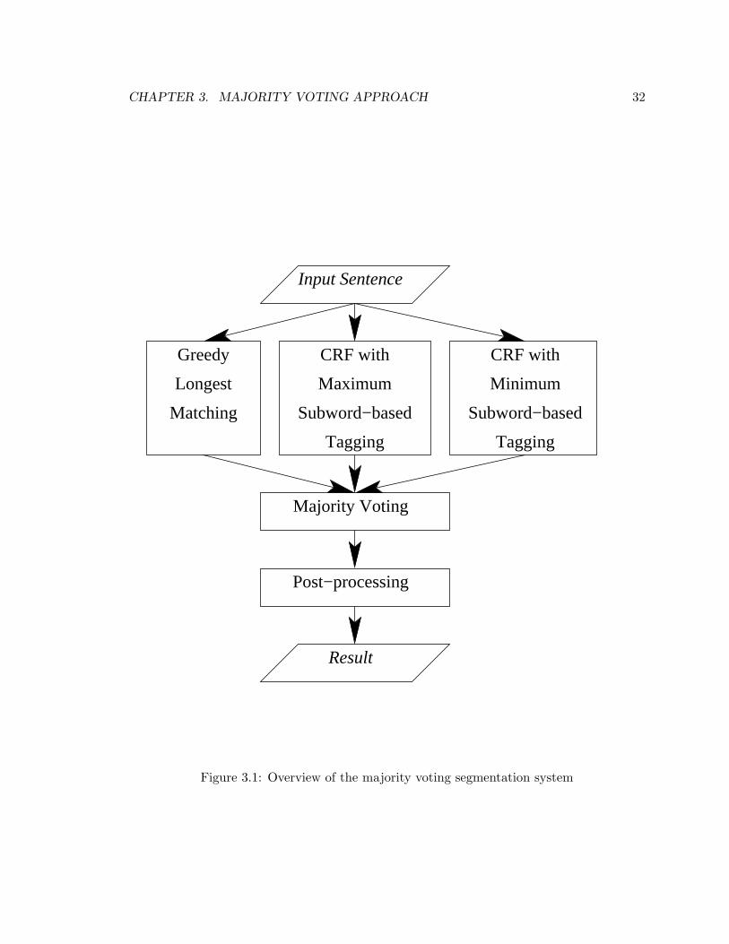
Our majority voting word segmentation system proceeds in three steps. In the first step, the
greedy longest matching method, which is a dictionary-based matching approach, is used
to generate a segmentation result. Also at the same time, the CRF model with maximum
subword-based tagging and the CRF model with minimum subword-based tagging, both of
which will be explained later in this chapter, are used individually to produce segmentation
results. In the second step, a character-level majority voting method takes these three seg-
mentation results as input and creates the initial output. In the last step, a post-processing
procedure is applied on this initial output to correct certain data inconsistency errors and
to get the final output. This post-processing procedure merges adjoining word candidates
to match with the dictionary entries and splits word candidates which are inconsistent with
entries in the training corpus. The overview of the whole system is shown in Figure 3.1.
This chapter is organized as follows: In Section 3.2, we provide a brief review of the
31
CHAPTER 3. MAJORITY VOTING APPROACH 32
Input Sentence
Longest
Greedy
Result
Post−processing
Majority Voting
Matching
CRF with
Maximum
Subword−based
Tagging
CRF with
Minimum
Subword−based
Tagging
Figure 3.1: Overview of the majority voting segmentation system

CHAPTER 3. MAJORITY VOTING APPROACH 33
greedy longest matching method. Section 3.3 describes the CRF model using maximum
subword-based tagging. Section 3.4 describes the CRF model using minimum subword-
based tagging, and in Section 3.5, the majority voting process is discussed. Section 3.6
talks about the post-processing step, attempting to correct the mistakes. Section 3.7 shows
the experimental results and analyzes the errors. Section 3.8 briefly discusses a modified
majority voting system in which minimum subword-based CRF-tagged candidate is substi-
tuted with character-based CRF-tagged candidate, while Section 3.9 summarizes this whole
chapter.
3.2 Greedy Longest Matching
Recall from Chapter 2 that the greedy longest matching algorithm is a dictionary-based
segmentation algorithm. It starts from the beginning of a sentence and proceeds through
the whole sentence, attempting to find the longest sub-sequence of characters matching any
dictionary word at each point. This algorithm is simple to understand, easy to implement,
efficient, and it maximizes the usage of dictionary. However, limited dictionary sizes com-
bined with frequent occurrences of unknown words become a major bottleneck if the greedy
longest matching approach is applied by itself.
3.3 CRF Model with Maximum Subword-based Tagging
Conditional random field, the discriminative sequence learning method, has been widely
used in various tasks [11, 21, 36, 55], including Chinese word segmentation [30, 52, 54].
In this approach, most existing systems apply the character-based tagger. For example,
“Ñ(all)/���(extremely important)” is labeled as “Ñ-O�-B�-I-I�-I”, using the
3-tagset.
In 2006, Zhang et al. [52] proposed a maximum subword-based “IOB” tagger for Chinese
word segmentation. This tagger proceeds as follows:
• First, the entire word list is extracted from the training corpus. Meanwhile, the
frequency count for each word in the list is recorded, and the words are sorted in
decreasing order according to their frequency count.
• Next, all the single-character words and the most frequent multi-character words are
extracted from this sorted list to form a lexicon subset.

CHAPTER 3. MAJORITY VOTING APPROACH 34
• Then, this subset is applied on the training data to tag the whole corpus in subword
format. For example, suppose we have the single-character words “Ñ”(all), “�”(to)
and “�”(close), and the most frequent multi-character word “�”(important) in
the lexical subset, then “Ñ/���” in the previous example is labeled as “Ñ-O
�-B �-I �-I” instead.
• After that, the tagged corpus is fed into CRF++, for training the discriminative model.
At the same time, the test data is segmented with the greedy longest matching method,
using the lexicon subset as the dictionary.
• In the last step, CRF++ labels these initially segmented test data, according to the
learnt model, to produce the final segmentation result.
We implemented this maximum subword-based CRF learning as one of our three systems
to produce an initial segmentation for majority voting. Also, in all our experiments, we
defined the most frequent words to be the top 5% in the sorted multi-character word list.
Zhang et al. [52] observed in their experiments that, with the CRF-based tagging approach,
a higher out-of-vocabulary recall rate is achieved, at the cost of getting a very low in-
vocabulary recall rate. We claim that the majority voting procedure will take advantage
of the dictionary information used in the greedy longest matching method and that of the
frequent word information used in this maximum subword-based CRF model to raise the
low in-vocabulary recall rate. Also, the voting procedure will benefit from the high out-of-
vocabulary recall rate achieved from the CRF-based tagging algorithms.
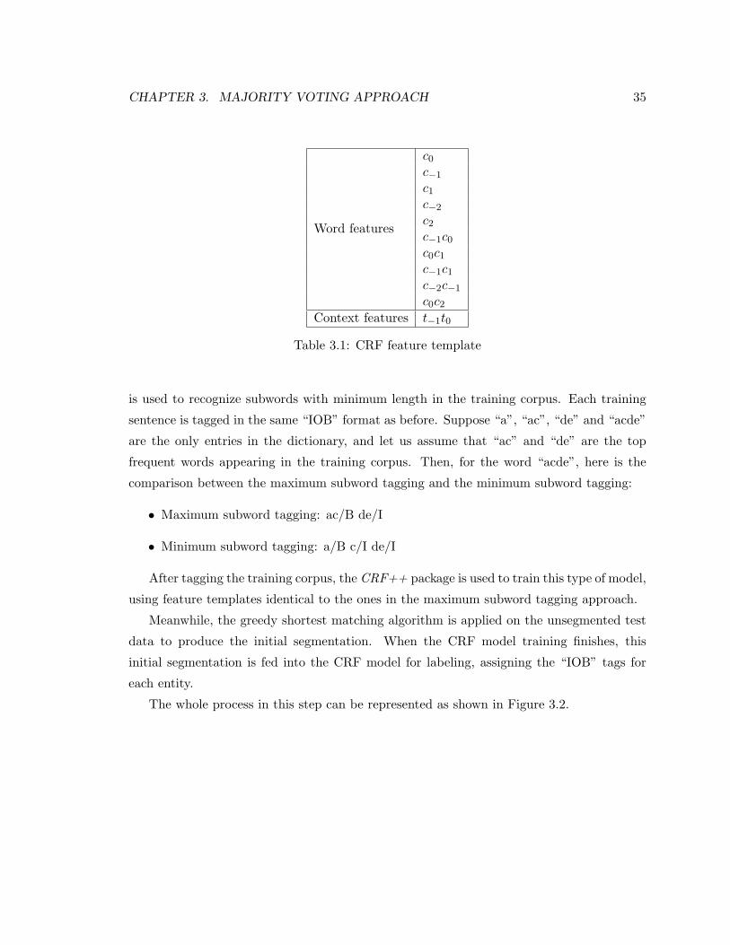
The feature template for sequence learning in this method and in all our CRF-related
experiments is adapted from [52] and summarized in Table 3.1, defining the symbol c to be
character in a character-based CRF method or word in a subword-based CRF method, and
defining the symbol t to be the observation. 0 means the current position; -1, -2, the first
or second position to the left; 1, 2, the first or second position to the right.
3.4 CRF Model with Minimum Subword-based Tagging
In our third model, we apply a similar approach as in the previous model. However, instead
of using the maximum subwords, we explore the minimum subword-based tagger. At the
beginning, we build the dictionary using the whole training corpus. Without extracting
the most frequent words as is done in the maximum subword tagger, the whole dictionary
CHAPTER 3. MAJORITY VOTING APPROACH 35
Word features
c0
c−1
c1
c−2
c2
c−1c0
c0c1
c−1c1
c−2c−1
c0c2
Context features t−1t0
Table 3.1: CRF feature template
is used to recognize subwords with minimum length in the training corpus. Each training
sentence is tagged in the same “IOB” format as before. Suppose “a”, “ac”, “de” and “acde”
are the only entries in the dictionary, and let us assume that “ac” and “de” are the top
frequent words appearing in the training corpus. Then, for the word “acde”, here is the
comparison between the maximum subword tagging and the minimum subword tagging:
• Maximum subword tagging: ac/B de/I
• Minimum subword tagging: a/B c/I de/I
After tagging the training corpus, the CRF++ package is used to train this type of model,
using feature templates identical to the ones in the maximum subword tagging approach.
Meanwhile, the greedy shortest matching algorithm is applied on the unsegmented test
data to produce the initial segmentation. When the CRF model training finishes, this
initial segmentation is fed into the CRF model for labeling, assigning the “IOB” tags for
each entity.
The whole process in this step can be represented as shown in Figure 3.2.

CHAPTER 3. MAJORITY VOTING APPROACH 36
Minimum SubwordTagging
CRF Decoding
Matching
Input Sentence
CRF Model
CRF Learning
Matching
Training Corpus
Output
Minimum Subword
Figure 3.2: Overview of the minimum subword-based tagging approach

CHAPTER 3. MAJORITY VOTING APPROACH 37
3.5 Character-level Majority Voting
3.5.1 The Voting Procedure
In this next step, with the segmentation results from the greedy longest matching, from the
CRF model with maximum subword-based tagging, and from the CRF model with minimum
subword-based tagging in hand, we apply the character-level majority voting algorithm.
First, for each character in a segmented sentence, we tag it either as “B” if it is the first
character of a word or a single-character word, or as “I” otherwise. (In word segmentation,
there is no “O” tag required – it can be always replaced with “B” tag. So for example,
“OBI” can be written as “BBI” without loss of information.) Then, for each corresponding
character from a specific sentence, if at least two of the models provide the same tag, that
specific tag will be assigned as the final tag for that character. For instance, considering the
character sequence “acde”, Table 3.2 illustrates the voting procedure. Suppose “a/c/de”
Method OutputGreedy Longest Matching a/B c/B d/B e/ICRF model with Maximum Subword Tagging a/B c/I d/I e/BCRF model with Minimum Subword Tagging a/B c/I d/B e/BVoting Result a/B c/I d/B e/B
Table 3.2: An example for the character-level majority voting
is the segmentation result from the greedy longest matching. “acd/e” is the result from
the CRF model with maximum subword-based tagging, and “ac/d/e” is the result from the
CRF model with minimum subword-based tagging. Then, for “a”, since all segmentation
results assign “B’ to it, “a” is tagged as “B”; for “c”, because two of the segmentation
methods tag it as “I”, “c” is tagged as “I”. Similarly, the tag for each remaining character
is determined by this majority voting process, and we get “ac/d/e” as the final output in
this example.
3.6 Post-processing Step
To test the performance of each of the three models and that of the majority voting, we
divide the MSRA corpus into a training set and a held-out set. The training set takes 80%

CHAPTER 3. MAJORITY VOTING APPROACH 38
of the whole MSRA training corpus sentences, and the held-out set takes the remaining
20% of the MSRA training corpus sentences. Table 3.3 shows the performance on the held-
out set. Throughout the experiments we conduct, we discover that those two CRF models
produced segmentation results with high F-scores, and that the voting process improves the
performance further.
P R F ROOV RIV
Greedy Longest Matching 91.9 95.7 93.7 2.1 98.3CRF with Maximum Subword Tagging 95.6 95.4 95.5 68.9 96.1CRF with Minimum Subword Tagging 95.5 95.0 95.3 68.6 95.8Majority Voting 96.2 96.3 96.2 65.2 97.1
Table 3.3: Performance (in percentage) on the MSRA held-out set
While analyzing errors with the segmentation result from the held-out set, we find two
types of inconsistency problem: first, the inconsistency between the dictionary and the
segmentation result: that is, certain characters that consistently appear together as a single
word in the dictionary are separated into consecutive word candidates in the test result.
Second, the inconsistency among words in the dictionary. For instance, both “)¦Ï
Ä”(scientific research) and “)¦(science)/ÏÄ(research)” appear in the training corpora,
reflecting different semantic meaning or being merely an error made by the human expert.
To deal with the first phenomena, for the segmented result, we merge adjoining word
candidates to match the dictionary entries, if the frequency of the adjoined word in the
training corpus is higher than that of the separated word sequence in the same corpus. Sup-
pose “a/b/c/de” is the original voting result, and the word “abc” appears more frequently
than the word sequence “a/b/c” in the training corpus. Then, we merge “a”, “b” and “c”
together to form the output “abc/de”.
For the second problem, we introduce the split procedure, which examines the word and
word sequence frequencies in the training corpus as well. In our system, we only consider
two consecutive word candidates. First, all word bigrams are extracted from the training
corpus, and their frequencies are counted. After that, for example, if the word bigram
“a/b” appears more often than the word candidate “ab”, then whenever in the test result
we encounter “ab”, we split it into “a/b”.
The post-processing steps detailed above take word and word sequence frequencies into

CHAPTER 3. MAJORITY VOTING APPROACH 39
consideration, attempt to maximize the value of known words in the training corpus as
well as deal with the word segmentation inconsistencies in the training corpus. The perfor-
mance after post-processing on MSRA held-out set is shown in Table 3.4 with bold numbers
representing the highest F-score. From the table, we see that, after post-processing, the
performance catches up with that produced by the character-based CRF method.
P R F ROOV RIV
Majority Voting 96.2 96.3 96.2 65.2 97.1After Post-Processing 96.5 96.4 96.5 65.2 97.3Character-based CRF 96.5 96.4 96.5 65.2 97.3
Table 3.4: Performance (in percentage) after post-processing on the MSRA heldout set
3.7 Experiments and Analysis
3.7.1 Experiment Corpora Statistics
The majority voting system is evaluated with the CityU corpus, the MSRA corpus, and the
UPUC corpus from the third SIGHAN bakeoff. The statistics, including sentence, word,
and character information for each training corpus, is summarized in Table 3.5. In addition,
Table 3.6 shows their corresponding test set sizes, counting the number of sentences.
CityU corpus MSRA corpus UPUC corpusNumber of Sentences 57, 275 46, 364 18, 804Number of Words 70, 290, 106 1, 266, 171 1, 144, 899Number of Word Types 151, 180 125, 266 74, 764Number of Characters 15, 074, 091 2, 169, 879 1, 235, 673Number of Character Types 10, 224 9, 534 8, 586
Table 3.5: Statistics for the CityU, MSRA and UPUC training corpora
3.7.2 Results on the Experiment Corpora
To observe the result of majority voting and the contribution of the post-processing step, the
experiment is run on each corpus by first producing the result of majority voting and then
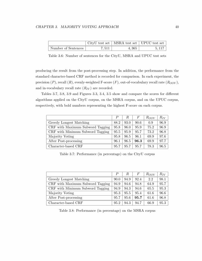
CHAPTER 3. MAJORITY VOTING APPROACH 40
CityU test set MSRA test set UPUC test setNumber of Sentences 7, 511 4, 365 5, 117
Table 3.6: Number of sentences for the CityU, MSRA and UPUC test sets
producing the result from the post-processing step. In addition, the performance from the
standard character-based CRF method is recorded for comparison. In each experiment, the
precision (P), recall (R), evenly-weighted F-score (F ), out-of-vocabulary recall rate (ROOV ),
and in-vocabulary recall rate (RIV ) are recorded.
Tables 3.7, 3.8, 3.9 and Figures 3.3, 3.4, 3.5 show and compare the scores for different
algorithms applied on the CityU corpus, on the MSRA corpus, and on the UPUC corpus,
respectively, with bold numbers representing the highest F-score on each corpus.
P R F ROOV RIV
Greedy Longest Matching 88.2 93.0 90.6 0.9 96.9CRF with Maximum Subword Tagging 95.8 96.0 95.9 75.2 96.9CRF with Minimum Subword Tagging 95.5 95.9 95.7 73.2 96.8Majority Voting 95.8 96.5 96.1 69.9 97.6After Post-processing 96.1 96.5 96.3 69.9 97.7Character-based CRF 95.7 95.7 95.7 78.3 96.5
Table 3.7: Performance (in percentage) on the CityU corpus
P R F ROOV RIV
Greedy Longest Matching 90.0 94.9 92.4 2.2 98.1CRF with Maximum Subword Tagging 94.9 94.6 94.8 64.9 95.7CRF with Minimum Subword Tagging 94.9 94.3 94.6 65.5 95.3Majority Voting 95.3 95.5 95.4 61.6 96.6After Post-processing 95.7 95.6 95.7 61.6 96.8Character-based CRF 95.2 94.3 94.7 66.9 95.3
Table 3.8: Performance (in percentage) on the MSRA corpus

CHAPTER 3. MAJORITY VOTING APPROACH 41
90
91
92
93
94
95
96
97
F-sc
ore
(in p
erce
ntag
e)Greedy LongestMatching
CRF with MaximumSubword Tagging
CRF with MinimumSubword Tagging
Majority Voting
After Post-processing
Character-based CRF
Figure 3.3: Comparison for F-scores on the CityU corpus, with histogram representation
92
92.5
93
93.5
94
94.5
95
95.5
96
F-sc
ore
(in p
erce
ntag
e)
Greedy LongestMatching
CRF with MaximumSubword Tagging
CRF with MinimumSubword Tagging
Majority Voting
After Post-processing
Character-based CRF
Figure 3.4: Comparison for F-scores on the MSRA corpus, with histogram representation

CHAPTER 3. MAJORITY VOTING APPROACH 42
P R F ROOV RIV
Greedy Longest Matching 79.0 86.9 82.8 1.1 95.1CRF with Maximum Subword Tagging 91.0 92.7 91.8 66.6 95.2CRF with Minimum Subword Tagging 90.8 92.5 91.7 66.9 95.0Majority Voting 90.9 93.2 92.0 63.0 96.1After Post-processing 91.0 93.2 92.1 62.9 96.0Character-based CRF 92.2 93.1 92.7 71.4 95.2
Table 3.9: Performance (in percentage) on the UPUC corpus
82
84
86
88
90
92
94
F-sc
ore
(in p
erce
ntag
e)
Greedy LongestMatching
CRF with MaximumSubword Tagging
CRF with MinimumSubword Tagging
Majority Voting
After Post-processing
Character-based CRF
Figure 3.5: Comparison for F-scores on the UPUC corpus, with histogram representation
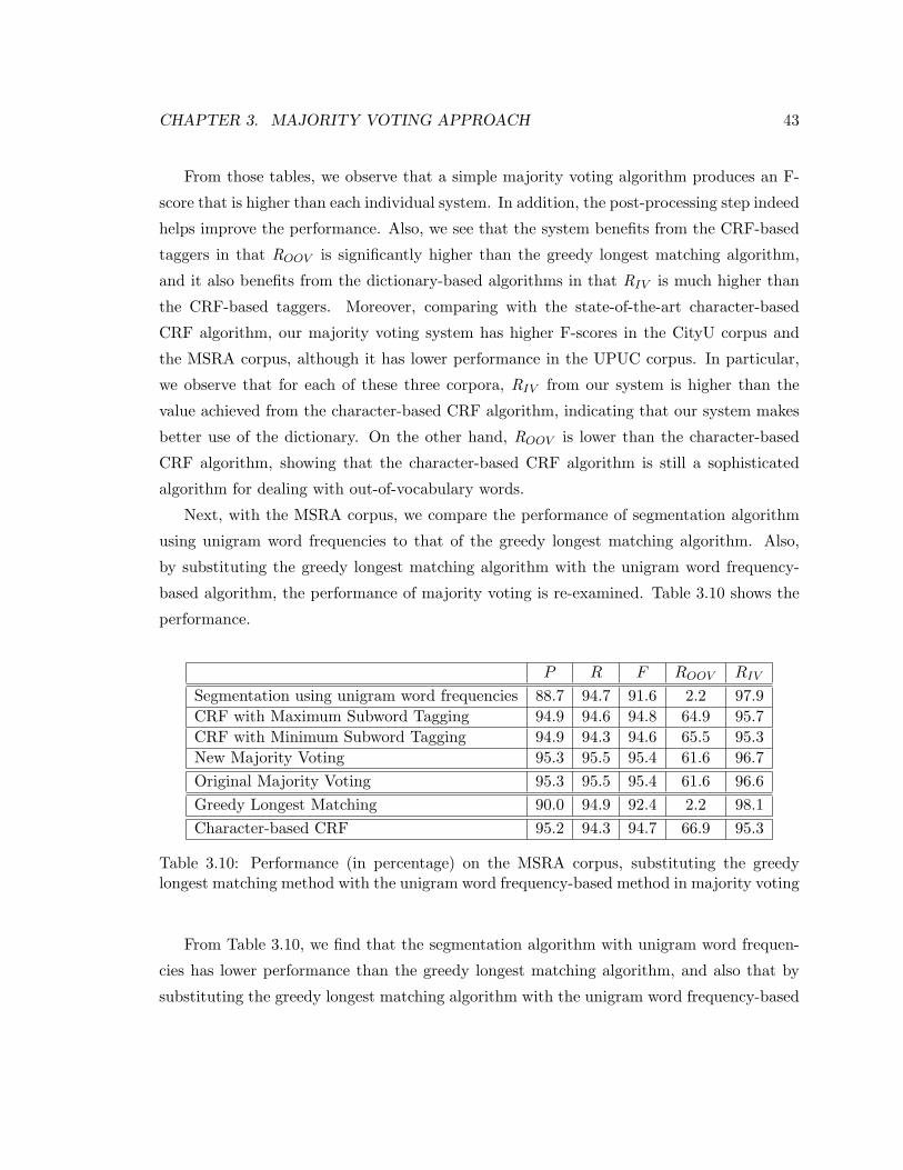
CHAPTER 3. MAJORITY VOTING APPROACH 43
From those tables, we observe that a simple majority voting algorithm produces an F-
score that is higher than each individual system. In addition, the post-processing step indeed
helps improve the performance. Also, we see that the system benefits from the CRF-based
taggers in that ROOV is significantly higher than the greedy longest matching algorithm,
and it also benefits from the dictionary-based algorithms in that RIV is much higher than
the CRF-based taggers. Moreover, comparing with the state-of-the-art character-based
CRF algorithm, our majority voting system has higher F-scores in the CityU corpus and
the MSRA corpus, although it has lower performance in the UPUC corpus. In particular,
we observe that for each of these three corpora, RIV from our system is higher than the
value achieved from the character-based CRF algorithm, indicating that our system makes
better use of the dictionary. On the other hand, ROOV is lower than the character-based
CRF algorithm, showing that the character-based CRF algorithm is still a sophisticated
algorithm for dealing with out-of-vocabulary words.
Next, with the MSRA corpus, we compare the performance of segmentation algorithm
using unigram word frequencies to that of the greedy longest matching algorithm. Also,
by substituting the greedy longest matching algorithm with the unigram word frequency-
based algorithm, the performance of majority voting is re-examined. Table 3.10 shows the
performance.
P R F ROOV RIV
Segmentation using unigram word frequencies 88.7 94.7 91.6 2.2 97.9CRF with Maximum Subword Tagging 94.9 94.6 94.8 64.9 95.7CRF with Minimum Subword Tagging 94.9 94.3 94.6 65.5 95.3New Majority Voting 95.3 95.5 95.4 61.6 96.7Original Majority Voting 95.3 95.5 95.4 61.6 96.6Greedy Longest Matching 90.0 94.9 92.4 2.2 98.1Character-based CRF 95.2 94.3 94.7 66.9 95.3
Table 3.10: Performance (in percentage) on the MSRA corpus, substituting the greedylongest matching method with the unigram word frequency-based method in majority voting
From Table 3.10, we find that the segmentation algorithm with unigram word frequen-
cies has lower performance than the greedy longest matching algorithm, and also that by
substituting the greedy longest matching algorithm with the unigram word frequency-based

CHAPTER 3. MAJORITY VOTING APPROACH 44
algorithm in majority voting, the F-score does not have any improvement. Thus, in the re-
maining experiments of this thesis, we will ignore the segmentation algorithm using unigram
word frequencies.
3.7.3 Error analysis
Examining the segmentation result from these three corpora, we find that the errors that
occur in the system are mainly caused by the following factors:
First, there is inconsistency between the gold segmentation and the training corpus,
and even within the training corpus or within the gold segmentation itself. Although the
inconsistency problem within the training corpus is intended to be tackled in the post-
processing step, we cannot conclude that the segmentation for certain words in the gold
test set always follows the convention in the training data set. Moreover, errors made
by human experts in the gold standard test set contribute to the inconsistency issue as
well. For instance, in the UPUC gold set, the person name “v]L”(Lai, Yingzhao) has
two distinct segmentations, “v/]L”, and “v]L”. In addition, the inconsistency issue,
perhaps as a result of some subtle context-based differences, is hard to model by current
methods. For example, in the MSRA training corpus, “¥)u�”(Chinese government)
and “¥)/u�” both appear, but in distinct surrounding context. Either of these two
segmentations is acceptable. For instance, in the phrase “¥)u�Z|ÌéqÄø)ßwf
e”(Chinese government and people are confident to achieve the goal), it is segmented as “¥
)(Chinese)/u�(government)/Z(and)/|Ì(people)/é(to)/qÄ(achieve)/ø)(goal)/ß
w(fulfill)/fe(confidence))” since the adjective “¥)”(Chinese) is related to both the
nouns “u�”(government) and “|Ì”(people). On the other hand, for the phrase “¥)u
��feqÄY�ø)”(Chinese government is confident to achieve this goal), “¥)u�”
is considered as a single unique entity and thus is not separated. This inconsistency issue
lowers the system performance.
Second, we don’t have specific steps to deal with words having common suffixes such as
“V”(person). Compared to our system, Zhang et al. [51] proposed a segmentation system
that contains a morphologically derived word recognition post-processing component to
solve this problem. We only focus on the closed track and thus we cannot include such a
step. This prevents us from identifying certain types of words such as “�ÄV”(worker).
In addition, unknown words are still troublesome because of the limited size of the
training corpora. In the class of unknown words, we encounter person names, numbers,
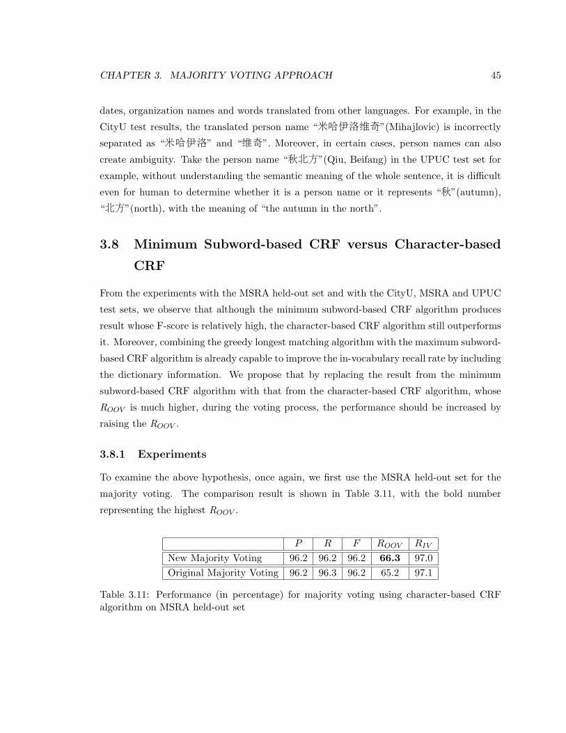
CHAPTER 3. MAJORITY VOTING APPROACH 45
dates, organization names and words translated from other languages. For example, in the
CityU test results, the translated person name “²-�b�Û”(Mihajlovic) is incorrectly
separated as “²-�b” and “�Û”. Moreover, in certain cases, person names can also
create ambiguity. Take the person name “Bð0”(Qiu, Beifang) in the UPUC test set for
example, without understanding the semantic meaning of the whole sentence, it is difficult
even for human to determine whether it is a person name or it represents “B”(autumn),
“ð0”(north), with the meaning of “the autumn in the north”.
3.8 Minimum Subword-based CRF versus Character-based
CRF
From the experiments with the MSRA held-out set and with the CityU, MSRA and UPUC
test sets, we observe that although the minimum subword-based CRF algorithm produces
result whose F-score is relatively high, the character-based CRF algorithm still outperforms
it. Moreover, combining the greedy longest matching algorithm with the maximum subword-
based CRF algorithm is already capable to improve the in-vocabulary recall rate by including
the dictionary information. We propose that by replacing the result from the minimum
subword-based CRF algorithm with that from the character-based CRF algorithm, whose
ROOV is much higher, during the voting process, the performance should be increased by
raising the ROOV .
3.8.1 Experiments
To examine the above hypothesis, once again, we first use the MSRA held-out set for the
majority voting. The comparison result is shown in Table 3.11, with the bold number
representing the highest ROOV .
P R F ROOV RIV
New Majority Voting 96.2 96.2 96.2 66.3 97.0Original Majority Voting 96.2 96.3 96.2 65.2 97.1
Table 3.11: Performance (in percentage) for majority voting using character-based CRFalgorithm on MSRA held-out set

CHAPTER 3. MAJORITY VOTING APPROACH 46
From the statistics, we see that, comparing with our previous voting strategy, after
voting, with sightly changes in R and RIV , ROOV increases more than 1%.
Then, we applied this new majority voting system with the CityU, MSRA and UPUC
test sets. Tables 3.12, 3.13, 3.14 and Figures 3.6, 3.7, 3.8 show and compare the scores for
different algorithms applied on the CityU corpus, on the MSRA corpus, and on the UPUC
corpus, respectively, with bold numbers representing the highest F-score on each corpus.
P R F ROOV RIV
Greedy Longest Matching 88.2 93.0 90.6 0.9 96.9CRF with Maximum Subword Tagging 95.8 96.0 95.9 75.2 96.9Character-based CRF 95.7 95.7 95.7 78.3 96.5New Majority Voting 96.3 96.6 96.4 74.1 97.5After Post-processing 96.5 96.6 96.6 74.1 97.6Original Majority Voting 95.8 96.5 96.1 69.9 97.6
Table 3.12: Performance (in percentage) on the CityU corpus, voting using the character-based CRF algorithm
P R F ROOV RIV
Greedy Longest Matching 90.0 94.9 92.4 2.2 98.1CRF with Maximum Subword Tagging 94.9 94.6 94.8 64.9 95.7Character-based CRF 95.2 94.3 94.7 66.9 95.3New Majority Voting 95.4 95.4 95.4 62.9 96.6After Post-processing 95.8 95.6 95.7 62.9 96.8Original Majority Voting 95.3 95.5 95.4 61.6 96.6
Table 3.13: Performance (in percentage) on the MSRA corpus, voting using the character-based CRF algorithm
We observe that by replacing the minimum subword-based CRF algorithm with the
character-based CRF algorithm during the voting process, the ROOV for the MSRA test set
increases 1.1%. Moreover, the F-score for the CityU test set increases 0.3%, and its ROOV
increases 4.2%. In addition, for the UPUC test set, its F-score even increases 0.7%, and its
ROOV increases 2.6%.

CHAPTER 3. MAJORITY VOTING APPROACH 47
90
91
92
93
94
95
96
97
F-sc
ore
(in p
erce
ntag
e)
Greedy Longest Matching
CRF with MaximumSubword Tagging
Character-based CRF
New Majority Voting
After Post-processing
Original Majority Voting
Figure 3.6: Comparison for F-scores on the CityU corpus, voting using the character-basedCRF algorithm, with histogram representation
92
92.5
93
93.5
94
94.5
95
95.5
96
F-sc
ore
(in p
erce
ntag
e)
Greedy Longest Matching
CRF with MaximumSubword Tagging
Character-based CRF
New Majority Voting
After Post-processing
Original Majority Voting
Figure 3.7: Comparison for F-scores on the MSRA corpus, voting using the character-basedCRF algorithm, with histogram representation

CHAPTER 3. MAJORITY VOTING APPROACH 48
P R F ROOV RIV
Greedy Longest Matching 79.0 86.9 82.8 1.1 95.1CRF with Maximum Subword Tagging 91.0 92.7 91.8 66.6 95.2Character-based CRF 92.2 93.1 92.7 71.4 95.2New Majority Voting 91.4 93.3 92.4 65.6 96.0Post-processing 91.5 93.3 92.4 65.6 96.0Original Majority Voting 90.9 93.2 92.0 63.0 96.1
Table 3.14: Performance (in percentage) on the UPUC corpus, voting using the character-based CRF algorithm
82
84
86
88
90
92
94
F-sc
ore
(in p
erce
ntag
e)
Greedy Longest Matching
CRF with MaximumSubword Tagging
Character-based CRF
New Majority Voting
After Post-processing
Original Majority Voting
Figure 3.8: Comparison for F-scores on the UPUC corpus, voting using the character-basedCRF algorithm, with histogram representation
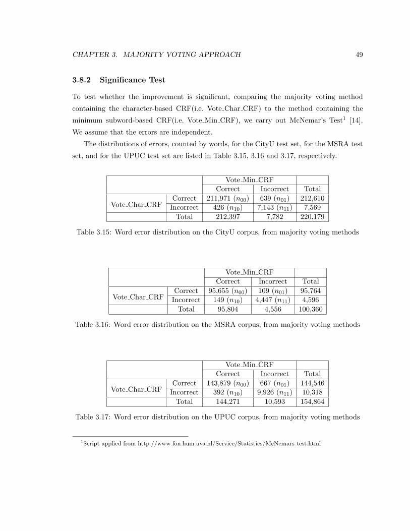
CHAPTER 3. MAJORITY VOTING APPROACH 49
3.8.2 Significance Test
To test whether the improvement is significant, comparing the majority voting method
containing the character-based CRF(i.e. Vote Char CRF) to the method containing the
minimum subword-based CRF(i.e. Vote Min CRF), we carry out McNemar’s Test1 [14].
We assume that the errors are independent.
The distributions of errors, counted by words, for the CityU test set, for the MSRA test
set, and for the UPUC test set are listed in Table 3.15, 3.16 and 3.17, respectively.
Vote Min CRFCorrect Incorrect Total
Vote Char CRFCorrect 211,971 (n00) 639 (n01) 212,610Incorrect 426 (n10) 7,143 (n11) 7,569
Total 212,397 7,782 220,179
Table 3.15: Word error distribution on the CityU corpus, from majority voting methods
Vote Min CRFCorrect Incorrect Total
Vote Char CRFCorrect 95,655 (n00) 109 (n01) 95,764Incorrect 149 (n10) 4,447 (n11) 4,596
Total 95,804 4,556 100,360
Table 3.16: Word error distribution on the MSRA corpus, from majority voting methods
Vote Min CRFCorrect Incorrect Total
Vote Char CRFCorrect 143,879 (n00) 667 (n01) 144,546Incorrect 392 (n10) 9,926 (n11) 10,318
Total 144,271 10,593 154,864
Table 3.17: Word error distribution on the UPUC corpus, from majority voting methods
1Script applied from http://www.fon.hum.uva.nl/Service/Statistics/McNemars test.html
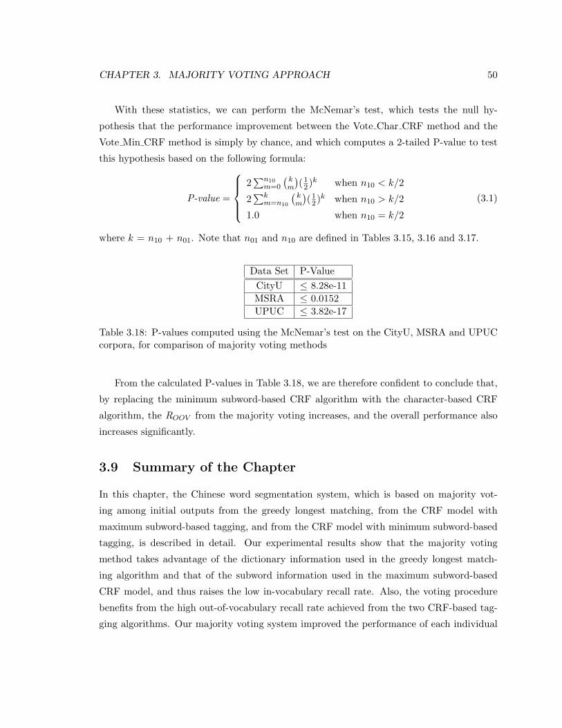
CHAPTER 3. MAJORITY VOTING APPROACH 50
With these statistics, we can perform the McNemar’s test, which tests the null hy-
pothesis that the performance improvement between the Vote Char CRF method and the
Vote Min CRF method is simply by chance, and which computes a 2-tailed P-value to test
this hypothesis based on the following formula:
P-value =
2∑n10
m=0
(km
)(12)k when n10 < k/2
2∑k
m=n10
(km
)(12)k when n10 > k/2
1.0 when n10 = k/2
(3.1)
where k = n10 + n01. Note that n01 and n10 are defined in Tables 3.15, 3.16 and 3.17.
Data Set P-ValueCityU ≤ 8.28e-11MSRA ≤ 0.0152UPUC ≤ 3.82e-17
Table 3.18: P-values computed using the McNemar’s test on the CityU, MSRA and UPUCcorpora, for comparison of majority voting methods
From the calculated P-values in Table 3.18, we are therefore confident to conclude that,
by replacing the minimum subword-based CRF algorithm with the character-based CRF
algorithm, the ROOV from the majority voting increases, and the overall performance also
increases significantly.
3.9 Summary of the Chapter
In this chapter, the Chinese word segmentation system, which is based on majority vot-
ing among initial outputs from the greedy longest matching, from the CRF model with
maximum subword-based tagging, and from the CRF model with minimum subword-based
tagging, is described in detail. Our experimental results show that the majority voting
method takes advantage of the dictionary information used in the greedy longest match-
ing algorithm and that of the subword information used in the maximum subword-based
CRF model, and thus raises the low in-vocabulary recall rate. Also, the voting procedure
benefits from the high out-of-vocabulary recall rate achieved from the two CRF-based tag-
ging algorithms. Our majority voting system improved the performance of each individual
CHAPTER 3. MAJORITY VOTING APPROACH 51
algorithm. In addition, we experimented with various steps in post-processing which effec-
tively improved the overall performance. Moreover, we examined that by substituting the
minimum subword-based CRF model with character-based CRF model during the majority
voting, we can make better usage of its higher out-of-vocabulary recall rate to raise ROOV
and the overall performance.

Chapter 4
Global Features and Global Linear
Models
In this chapter, we propose the use of global features to assist with local features in training
an averaged perceptron on N-best candidates for Chinese word segmentation. Our experi-
ments show that by adding global features, performance is significantly improved compared
to the character-based CRF tagger. Performance is also improved compared to using only
local features. Testing on the closed track of the CityU, MSRA and UPUC corpora from
the third SIGHAN bakeoff, our system obtains a significant improvement in F-score from
95.7% to 97.1%, from 95.2% to 95.8%, and from 92.8% to 93.1%, respectively, comparing
with the character-based CRF tagger.
The chapter is organized as follows: Section 4.1 provides an overview of the system;
Section 4.2 describes the system architecture in depth; Section 4.3 shows and analyzes the
experimental results; Section 4.4 explores the weight learning for global features; Section 4.5
compares the N-best list re-ranking method with the beam search decoding approach; while
Section 4.6 briefly explores another global linear model – the exponential gradient learning
approach; Section 4.7 discusses related works, and Section 4.8 gives the summary for this
chapter.
52

CHAPTER 4. GLOBAL FEATURES AND GLOBAL LINEAR MODELS 53
4.1 Averaged Perceptron Global Linear Model
Our averaged perceptron word segmentation system implements the re-ranking technique.
The overview of the entire system is shown in Figure 4.1. For each of the training corpora,
we produce a 10-fold split: in each fold, 90% of the corpus is used for training and 10% is
used to produce an N-best list of candidates. The N-best list is produced using a character-
based CRF tagger. The true segmentation can now be compared with the N-best list in
order to train with an averaged perceptron algorithm. This system is then used to predict
the best word segmentation from an N-best list for each sentence in the test data.
Training Corpus
Weight Vector
N−best Candidates
Training With
Decoding With
Conditional Random
N−best Candidates
Field
Local Features Global Features
Average PerceptronInput Sentence
Average Perceptron
Output
Conditional RandomField
(10−Fold Split)
Figure 4.1: Overview of the averaged perceptron system

CHAPTER 4. GLOBAL FEATURES AND GLOBAL LINEAR MODELS 54
4.2 Detailed System Description
Recall from Chapter 2 that, given an unsegmented sentence x, the Chinese word segmenta-
tion problem can be defined as finding the most plausible output sentence F (x ) from a set
of possible segmentations of x :
F (x ) = argmaxy∈GEN(x)
Φ(x, y) ·w
where GEN (x ) is the set of possible segmentations for the input sentence x. The weight
parameter vector w, being initially set to 0, is maintained and updated while iterating
through the training set during the perceptron learning process (See Figure 2.10).
In our system, the averaged perceptron algorithm, which is capable of reducing over-
fitting on the training data and producing a more stable solution, is implemented. Also, the
lazy update process is adapted to reduce the time taken for training.
4.2.1 N-best Candidate List
In Figure 2.10, in order to calculate GEN(xi) in argmaxy∈GEN(xi), the naıve method can be
implemented to first generate all possible segmented candidates for the character sequence.
For a sentence with L characters, there are 2L−1 possible segmentations. For example,
suppose we have a sentence with 3 characters “abc”, then the following 4 candidates are to
be generated: “abc”, “a/bc”, “ab/c”, and “a/b/c”. When L is large, however, generating
those segmentations and picking the one with the highest score is time consuming. For
instance, if L=20, then over 500,000 candidates are required to be produced and examined.
Our system makes use of the re-ranking approach. Re-ranking has been broadly applied
in various natural language tasks such as parsing [6] and machine translation [38]. The
general intuition of any re-ranking method is to apply a separate model to re-rank the
output of a base system. For each input sentence, this base system produces a set of
candidate outputs, and defines an initial ranking for these candidates. The second model
attempts to improve upon this initial ranking so that candidates that are closer to the truth
get a higher rank. In our system, only a small portion of all possible segmentations, that
is, the N-best ranked candidate segmentations, are produced by the CRF++ package, and
the perceptron learning model tends to re-rank these candidates to pick the one closest to
the truth.

CHAPTER 4. GLOBAL FEATURES AND GLOBAL LINEAR MODELS 55
We use the standard method for producing N-best candidates in order to train our re-
ranker which uses global and local features: 10-folds of training data are used to train the
tagger on 90% of the data and then produce N-best lists for the remaining 10%. This process
gives us an N-best candidate list for each sentence and the candidate that is most similar
to the true segmentation, called yb. Notice that in this modeling process, the characters in
the training sentences are assigned “BMES” tags1, and the same feature templates listed in
Table 3.1 are applied in CRF tagging.
Figure 4.2 shows the modified averaged perceptron algorithm on the N-best candidate
list.
Inputs: Training Data 〈(x1, y1), . . . , (xm, ym)〉; number of iterations TInitialization: Set w = 0, γ = 0, σ = 0Algorithm:
for t = 1, . . . , T dofor i = 1, . . . ,m do
Calculate y′i, where y
′i = argmax
y∈N-best CandidatesΦ(y) ·w
if y′i 6= yb then
w = w + Φ(yb)− Φ(y′i)
end ifσ = σ + w
end forend for
Output: The averaged weight parameter vector γ = σ/(mT)
Figure 4.2: The averaged perceptron learning algorithm on the N-best list
4.2.2 Feature Templates
The feature templates used in our system include both local features and global features.
For local features, the 14 feature types from Zhang and Clark’s paper [53] in ACL 2007 are
adapted, and they are shown in Table 4.1.
While a local feature indicates the occurrence of a certain pattern in a partially seg-
mented sentence, a global feature provides information about the entire sentence. Our
1Performance of the CRF tagger might be improved with the use of other tagsets. However, this doesnot affect our comparative experiments
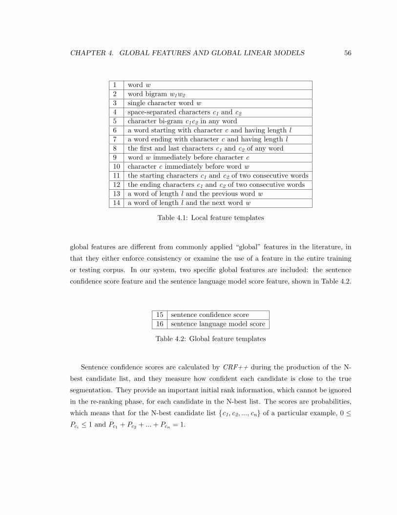
CHAPTER 4. GLOBAL FEATURES AND GLOBAL LINEAR MODELS 56
1 word w2 word bigram w1w2
3 single character word w4 space-separated characters c1 and c2
5 character bi-gram c1c2 in any word6 a word starting with character c and having length l7 a word ending with character c and having length l8 the first and last characters c1 and c2 of any word9 word w immediately before character c10 character c immediately before word w11 the starting characters c1 and c2 of two consecutive words12 the ending characters c1 and c2 of two consecutive words13 a word of length l and the previous word w14 a word of length l and the next word w
Table 4.1: Local feature templates
global features are different from commonly applied “global” features in the literature, in
that they either enforce consistency or examine the use of a feature in the entire training
or testing corpus. In our system, two specific global features are included: the sentence
confidence score feature and the sentence language model score feature, shown in Table 4.2.
15 sentence confidence score16 sentence language model score
Table 4.2: Global feature templates
Sentence confidence scores are calculated by CRF++ during the production of the N-
best candidate list, and they measure how confident each candidate is close to the true
segmentation. They provide an important initial rank information, which cannot be ignored
in the re-ranking phase, for each candidate in the N-best list. The scores are probabilities,
which means that for the N-best candidate list {c1, c2, ..., cn} of a particular example, 0 ≤Pci ≤ 1 and Pc1 + Pc2 + ... + Pcn = 1.

CHAPTER 4. GLOBAL FEATURES AND GLOBAL LINEAR MODELS 57
Sentence language model scores are produced using the SRILM [41] toolkit2. They
indicate how likely a sentence can be generated given the training data, and they help
capture the usefulness of features extracted from the training data. The n-gram word
statistics, where n is between 1 and 3, for the whole training corpus, is generated by this
toolkit and is then applied on each N-best candidate to calculate its language model score.
It is normalized using the formula P1/L, where P is the probability-based language model
score and L is the length of the sentence in words (not in characters). Since SRILM returns
the score in log-probability form, the value we will use for this feature is | (log(P))/L |.In our perceptron learning process, the weights for local features are updated so that
whenever a mismatch is found between the best candidate yb and the current top-scored
candidate Ctop, the weight parameter values for features in yb are incremented, and the
weight parameter values for features appearing in Ctop are decremented. For the global
features, however, their weights are not learned using the perceptron algorithm but are
determined using a development set.
4.2.3 A Perceptron Learning Example with N-best Candidate List
To illustrate the process of perceptron training using N-best candidate list, we provide an
example for weight learning, assuming that only local features are applied and that the
weights for global features are all zero. For simplicity, only Features 1–5 in Table 4.1 are
applied in this example.
Suppose the whole training set only contains one training example, and its N-best list
includes 6-best possible segmentation sentences, as shown below, and the number of iteration
t is set to be 3:
• The Best Candidate: ·¢(we)/Ù(live)/ó(in)/få(information)/�S(age)
• Candidate 1: ·¢(we)/(born)/Ù(alive)/ó(in)/få(information)/�S(age)
• Candidate 2: ·¢(we)/Ùó(live in)/få(information)/�S(age)
• Candidate 3: ·¢(we)/Ù(live)/ó(in)/få�S(information age)
• Candidate 4: ·¢(we)/Ùó(live in)/få�S(information age)
2available from http://www.speech.sri.com/projects/srilm/

CHAPTER 4. GLOBAL FEATURES AND GLOBAL LINEAR MODELS 58
• Candidate 5: ·¢(we)/(born)/Ù(alive)/ó(in)/få�S(information age)
• Candidate 6: ·¢(we)/Ù(live)/ó(in)/få(information)/�S(age)
During the first iteration, since w is initialized to zero, all those six candidates have
equal possibility of being chosen as the top-scored one because the score for each of them
is zero. We choose Candidate 1 to be our candidate. Comparing the best candidate and
Candidate 1,
• The Best Candidate: ·¢(we)/Ù(live)/ó(in)/få(information)/�S(age)
• Candidate 1: ·¢(we)/(born)/Ù(alive)/ó(in)/få(information)/�S(age)
we see that they are not identical. Thus, we reward features appearing in the best candidate
and penalize features in this chosen candidate, and achieve the following weight vector w1:
F1Ù(live) : 1 (born) : -1Ù(alive) : -1(·¢(we), Ù(live)) : 1 (Ù(live), ó(in)) : 1
F2 (·¢(we), (born)) : -1 ((born), Ù(alive)) : -1(Ù(alive), ó(in)) : -1
F3 (born) : -1 Ù(alive) : -1F4 ((born), Ù(alive)) : -1F5 ((born), Ù(alive)) : 1
Table 4.3: Updated weight vector w1 in the perceptron learning example
In the second iteration, each candidate in the 6-best list is re-scored using this updated
weight vector. For example, for Candidate 3, its weight corresponding to each feature is
summarized to be:
• Weight for F1 in Sentence 3: Ù(live) : 1
• Weight for F2 in Sentence 3: (·¢(we), Ù(live)) : 1 ; (Ù(live), ó(in)) : 1
• Weight for F5 in Sentence 3: ((born), Ù(alive)) : 1
Therefore, the score for Candidate 3 is 4 (i.e. Score(s3) = 4). Similarly, we calculate
scores for the remaining sentences in this 6-best list, and get Score(s1) = -8, Score(s2) = 1,
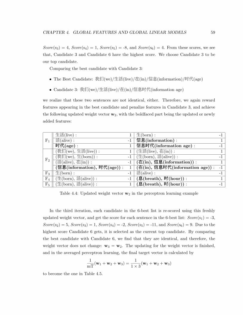
CHAPTER 4. GLOBAL FEATURES AND GLOBAL LINEAR MODELS 59
Score(s3) = 4, Score(s4) = 1, Score(s5) = -8, and Score(s6) = 4. From these scores, we see
that, Candidate 3 and Candidate 6 have the highest score. We choose Candidate 3 to be
our top candidate.
Comparing the best candidate with Candidate 3:
• The Best Candidate: ·¢(we)/Ù(live)/ó(in)/få(information)/�S(age)
• Candidate 3: ·¢(we)/Ù(live)/ó(in)/få�S(information age)
we realize that these two sentences are not identical, either. Therefore, we again reward
features appearing in the best candidate and penalize features in Candidate 3, and achieve
the following updated weight vector w2, with the boldfaced part being the updated or newly
added features:
Ù(live) : 1 (born) : -1F1 Ù(alive) : -1 fffååå(information) : 1
���SSS(age) : 1 fffååå���SSS(information age) : -1(·¢(we), Ù(live)) : 1 (Ù(live), ó(in)) : 1
F2(·¢(we), (born)) : -1 ((born), Ù(alive)) : -1(Ù(alive), ó(in)) : -1 (óóó(in), fffååå(information)) : 1(fffååå(information), ���SSS(age)) : 1 (óóó(in), fffååå���SSS(information age)) : -1
F3 (born) : -1 Ù(alive) : -1F4 ((born), Ù(alive)) : -1 (ååå(breath), ���(hour)) : 1F5 ((born), Ù(alive)) : 1 (ååå(breath), ���(hour)) : -1
Table 4.4: Updated weight vector w2 in the perceptron learning example
In the third iteration, each candidate in the 6-best list is re-scored using this freshly
updated weight vector, and get the score for each sentence in the 6-best list: Score(s1) = -3,
Score(s2) = 5, Score(s3) = 1, Score(s4) = -2, Score(s5) = -11, and Score(s6) = 9. Due to the
highest score Candidate 6 gets, it is selected as the current top candidate. By comparing
the best candidate with Candidate 6, we find that they are identical, and therefore, the
weight vector does not change: w3 = w2. The updating for the weight vector is finished,
and in the averaged perceptron learning, the final target vector is calculated by
1mT
(w1 + w2 + w3) =1
1× 3(w1 + w2 + w3)
to become the one in Table 4.5.

CHAPTER 4. GLOBAL FEATURES AND GLOBAL LINEAR MODELS 60
Ù(live) : 1 (born) : -1F1 Ù(alive) : -1 få(information) : 2/3
�S(age) : 2/3 få�S(information age) : -2/3(·¢(we), Ù(live)) : 1 (Ù(live), ó(in)) : 1
F2(·¢(we), (born)) : -1 ((born), Ù(alive)) : -1(Ù(alive), ó(in)) : -1 (ó(in), få(information)) : 2/3(få(information), �S(age)) : 2/3 (ó(in), få�S(information age)) : -2/3
F3 (born) : -1 Ù(alive) : -1F4 ((born), Ù(alive)) : -1 (å(breath), �(hour)) : 2/3F5 ((born), Ù(alive)) : 1 (å(breath), �(hour)) : -2/3
Table 4.5: Final weight vector in the perceptron learning example
4.3 Experiments
To test the performance of our system, the CityU, MSRA and UPUC corpora from the third
SIGHAN bakeoff are used once again, following the closed track.
4.3.1 Parameter Pruning
First, we experimented on the development set of the UPUC corpus to find a suitable value
for the parameter n, the maximum number of N-best candidates. This oracle procedure
proceeds as follows: 80% of the training corpus is used to train the CRF model, which is used
to produce the N-best outputs for each sentence on the remaining 20% of the corpus. Then,
these N candidates are compared with the true segmentation, and for each training sentence,
the candidate closest to the truth is chosen as the final output. As we increase the value of
n, for some sentences, its n-best candidate list is more likely to contain a segmentation that
will improve the overall F-score (Figure 4.3). However, the cost of choosing a larger value
of n leads to increased time complexity in the perceptron learning algorithm. To balance
accuracy and speed, we choose n to be 20 in all remaining experiments.
Next, the weight for sentence confidence score Scrf and that for language model score
Slm are determined. In this step, each training corpus is separated into a training set, which
contains 80% of the training corpus, and a development set containing the remaining 20%
of the training corpus. Then, the perceptron algorithm is applied on the training set with
different Scrf and Slm weight values, and for various number of iterations. The weight values

CHAPTER 4. GLOBAL FEATURES AND GLOBAL LINEAR MODELS 61
94
95
96
97
98
99
100
0 5 10 15 20 25 30 35 40 45 50
F-s
core
(in
per
cent
age)
Number of Maximum Candidate
F-score
Figure 4.3: F-score on the UPUC development set with different n
we test include 2, 4, 6, 8, 10, 15, 20, 30, 40, 50, 100 and 200, across a wide range of scales. As
we can see, there will be a significant number of testing scenarios (i.e. 12×12 = 144 testing
scenarios) in order to pick the most suitable weight values for each corpus. To simplify the
process, we assume that the weights for both Scrf and Slm are equal. Figures 4.4, 4.5, 4.6
show the F-scores on each of the three corpora using different Scrf and Slm weight values
with different number of iterations t. From the tables, we observe that when the weight for
Scrf and Slm increases, F-score improves; however, if the weight for Scrf and Slm becomes too
large to overrule the effect of weight learning on local features, F-score drops down. For the
remaining experiments, the weight for Scrf and Slm is chosen to be 15 for the CityU corpus,
to be 15 for the MSRA corpus, and to be 20 for the UPUC corpus.
While determining the weights for global features, the number of training iterations can
be determined as well. The trends from Figures 4.4, 4.5, 4.6 show that, as the number of
iterations increases, F-score stabilizes for most cases, reflecting convergence of the learning
algorithm. From the learning curves, we can fix the number of training iterations to be 7
for the CityU and MSRA corpora, and to be 9 for the UPUC corpus.

CHAPTER 4. GLOBAL FEATURES AND GLOBAL LINEAR MODELS 62
96.6
96.8
97
97.2
97.4
97.6
97.8
1 2 3 4 5 6 7 8 9 10
F-s
core
(in
per
cent
age)
Iterations
2
4,200
6,8,10,100
15,20,30,40,50
w=2
w=4
w=6
w=8
w=10
w=15
w=20
w=30
w=40
w=50
w=100
w=200
Figure 4.4: F-scores on the CityU development set
95.2
95.4
95.6
95.8
96
96.2
96.4
96.6
96.8
1 2 3 4 5 6 7 8 9 10
F-s
core
(in
per
cent
age)
Iterations
2
4
6,200
8,10,100
15,20,30,40,50
w=2w=4
w=6w=8
w=10w=15
w=20w=30
w=40w=50
w=100w=200
Figure 4.5: F-scores on the MSRA development set

CHAPTER 4. GLOBAL FEATURES AND GLOBAL LINEAR MODELS 63
94.6
94.8
95
95.2
95.4
95.6
95.8
96
1 2 3 4 5 6 7 8 9 10
F-s
core
(in
per
cent
age)
Iterations
2
4,200
6,8,100
10,15,30,40,5020
w=2w=4
w=6w=8
w=10w=15
w=20w=30
w=40w=50
w=100w=200
Figure 4.6: F-scores on the UPUC development set
4.3.2 Experiment Results
The performance is measured using F-score(F ), precision(P), recall(R), in-vocabulary recall
rate(RIV) and out-of-vocabulary recall rate(ROOV). We compare our approach with the
averaged perceptron using only local features, the character-based CRF method, and the
base-line performance using the greedy longest matching method, and the results are listed
in the Table 4.6. For each corpus, the bold number shows the highest F-score. Figure 4.7
intuitively compares the F-score results among these various methods.
From these experimental results, we see that our system outperforms the dictionary-
based greedy longest matching method. Also, our system improves the performance of the
character-based CRF. In addition, using global features, our model achieved better overall
performance than the perceptron algorithm using only local features.
4.3.3 Significance Test
To test whether the improvement is significant, compared to the character-based one-best
CRF result, we carry out McNemar’s test and assume that the errors are independent.

CHAPTER 4. GLOBAL FEATURES AND GLOBAL LINEAR MODELS 64
Corpus Setting F P R RIV ROOV
CityU
Averaged Perceptron with globaland local features
97.1 97.1 97.1 97.9 78.3
Averaged Perceptron with only localfeatures
96.7 96.7 96.6 97.5 77.4
Character-based conditional randomfield
95.7 95.7 95.8 96.6 77.7
Greedy longest matching 90.6 88.2 93.0 96.9 0.9
MSRA
Averaged Perceptron with globaland local features
95.8 95.9 95.7 96.9 62.0
Averaged Perceptron with only localfeatures
95.5 95.6 95.3 96.3 65.4
Character-based conditional randomfield
95.2 95.6 94.8 95.8 67.1
Greedy longest matching 92.4 90.0 94.9 98.1 2.2
UPUC
Averaged Perceptron with globaland local features
93.1 92.5 93.8 96.1 69.4
Averaged Perceptron with only localfeatures
92.5 91.8 93.1 95.5 68.8
Character-based conditional randomfield
92.8 92.2 93.3 95.5 70.9
Greedy longest matching 82.8 79.0 86.9 95.1 1.1
Table 4.6: Performance (in percentage) on CityU, MSRA, and UPUC Corpora

CHAPTER 4. GLOBAL FEATURES AND GLOBAL LINEAR MODELS 65
82
84
86
88
90
92
94
96
98
CityU MSRA UPUC
F-sc
ore
(in p
erce
ntag
e)
Averaged Perceptron withglobal and local features
Averaged Perceptron withonly local features
Character-basedconditional random field
Greedy Longest Matching
Figure 4.7: Comparison for F-scores on the CityU, MSRA, and UPUC corpora, with his-togram representation
The distributions of the errors, counted by words, for the CityU test set, for the MSRA
test set, and for the UPUC test set are listed in Table 4.7, 4.8 and 4.9, respectively.
one-best CRF resultCorrect Incorrect Total
perceptron re-rankingCorrect 209,583 (n00) 4,175 (n01) 213,758Incorrect 1,337 (n10) 5,084 (n11) 6,421
Total 210,920 9,259 220,179
Table 4.7: Word error distribution on the CityU corpus
With these statistics, we can perform the McNemar’s test, which tests the null hypothesis
that the performance improvement between the global-feature-based averaged perceptron
and the character-based CRF is simply by chance, and which computes a 2-tailed P-value
to test this hypothesis.
From the calculated P-value in Table 4.10, we are therefore confident to conclude that, for
all CityU, MSRA and UPUC test sets, the difference in performance between the averaged
perceptron using global features and the character-based CRF is significant.

CHAPTER 4. GLOBAL FEATURES AND GLOBAL LINEAR MODELS 66
one-best CRF resultCorrect Incorrect Total
perceptron re-rankingCorrect 94,308 (n00) 1,763 (n01) 96,071Incorrect 835 (n10) 3,454 (n11) 4,289
Total 95,143 5,217 100,360
Table 4.8: Word error distribution on the MSRA corpus
one-best CRF resultCorrect Incorrect Total
perceptron re-rankingCorrect 142,581 (n00) 2,636 (n01) 145,217Incorrect 1,932 (n10) 7,715 (n11) 9,647
Total 144,513 10,351 154,864
Table 4.9: Word error distribution on the UPUC corpus
Data Set P-ValueCityU ≤ 2.04e-319MSRA ≤ 7e-74UPUC ≤ 2.5e-25
Table 4.10: P-values computed using the McNemar’s test on the CityU, MSRA and UPUCcorpora, for comparison between the averaged perceptron using global features and thecharacter-based CRF

CHAPTER 4. GLOBAL FEATURES AND GLOBAL LINEAR MODELS 67
4.3.4 Error Analysis
By analyzing segmentation results, we discover that, for the CityU output, errors repeatedly
involve punctuation as well as numbers. For instance, the front double quote in [“/��/”] is
mistakenly combined with its following word to become [“��/”]. As another example, the
number “18” as in “18/�”(the 18th day in a month) in certain sentences is broken into two
words “1” and “8”. However, we notice that these errors also happen in the output produced
by character-based conditional random field, from which our N-best list is generated.
In addition to punctuation and number errors, personal names are another major source
of errors, not only in the CityU output, but also in the MSRA as well as the UPUC seg-
mentation results.
While for the UPUC output, the suffix character “R”(date) as in “5Û/15R”(May 15th)
also tends to cause errors to happen. In the UPUC’s training set, the character “R” with
the context of “date” seldom occurs; therefore, there are few patterns that contain “R” and
thus, not only for producing N-best candidates using CRF++ but also in weight update
during perceptron learning, its related patterns cannot be emphasized. However, this suffix
frequently appears in the test set, and it is therefore segmented incorrectly (e.g. to become
“15/R”).
4.4 Global Feature Weight Learning
The word segmentation system, designed by Liang in [26], incorporated and learned the
weights for mutual information (MI) features, whose values are continuous. In the weight
learning process, in order to deal with the mismatch between continuous and binary features,
Liang transformed the MI values into either of the following forms:
• Scale the MI values into some fixed range [a, b], where the smallest MI value maps to
a, and the largest MI value maps to b.
• Apply z-scores instead of their original MI values. The z-score of an MI value x is
defined as x−µσ where µ and σ represent the mean and standard deviation of the MI
distribution, respectively.
• Map any MI value x to a if x < µ, the mean MI value, or to b if x ≥ µ.

CHAPTER 4. GLOBAL FEATURES AND GLOBAL LINEAR MODELS 68
Testing with those various transformations, Liang shows that the weight for the MI
feature can be learned in the same way as the weight for the binary features and that the
word segmentation performance increases by normalizing the MI values. Especially, the
highest increase is obtained by normalizing them with z-scores.
For our global features, both sentence confidence score and sentence language model
score have the property that their values are also continuous rather than discrete. There-
fore, we try to see whether Liang’s method to incorporate MI features could be applied to
automatically learn weights for our two global features during perceptron training, instead
of manually fixing their weight using the development set.
We experiment with the transformations on those two global features with the UPUC
and CityU corpora. Table 4.11 provides the performance on their development sets as well
as test sets.
Method F-score (UPUC corpus) F-score (CityU corpus)held-out set test set held-out set test set
Without global features 95.5 92.5 97.3 96.7Fixed global feature weights 96.0 93.1 97.7 97.1Threshold at mean to 0,1 95.0 92.0 96.7 96.0Threshold at mean to -1,1 95.0 92.0 96.6 95.9Normalize to [0,1] 95.2 92.1 96.8 96.0Normalize to [-1,1] 95.1 92.0 96.8 95.9Normalize to [-3,3] 95.1 92.1 96.8 96.0Z-score 95.4 92.5 97.1 96.3
Table 4.11: F-scores (in percentage) obtained by using various ways to transform globalfeature weights and by updating their weights in averaged perceptron learning. The exper-iments are done on the UPUC and CityU corpora.
Different transformations give different performance. Among the normalization meth-
ods, the one with z-scores has the highest F-score. However, all of those accuracies are worse
than our previous method for fixing global feature weights using the development set. As
a result, better methods to perform weight updates for global features need to be explored
further in the future.

CHAPTER 4. GLOBAL FEATURES AND GLOBAL LINEAR MODELS 69
4.5 Comparison to Beam Search Decoding
4.5.1 Beam search decoding
In Zhang and Clark’s paper [53], instead of applying the N-best re-ranking method, their
word segmentation system adapts beam search decoding [10, 33], using only local features.
In beam search, the decoder generates segmentation candidates incrementally. It reads
one character at a time from the input sentence, and combines it with each existing candidate
in two ways, either appending this new character to the last word, or considering it as the
beginning of a new word. This combination process generates segmentations exhaustively;
that is, for a sentence with k characters, all 2k−1 possible segmentations are generated.
We implemented the decoding algorithm following the pseudo-code described by Zhang
and Clark [53]. According to their pseudo-code (see Figure 4.8), one source agenda and one
target agenda, both being initially empty, are used. In each step, the decoder combines the
character read from the input sentence with each candidate in the source agenda, and puts
the results into the target agenda. After processing the current character, the source agenda
is cleared, each item in the target agenda is copied back into the source agenda to form the
new candidates which will be used to process the next character, and then, the target agenda
is cleared. After the last character in the current input sentence is processed, the candidate
with the best score in the source agenda is returned by the decoder for training the averaged
perceptron.
To guarantee reasonable running speed, the beam size is limited to be B, a value that is
usually much less than 2k−1, which means that after processing each character, only the B
best candidates are preserved.
4.5.2 Experiments
During training with the Peking University corpus (PU), which contains 19,056 sentences,
from the first SIGHAN bakeoff, we observe that the running speed for this beam search
decoding based segmentation system is low. To examine whether we can use only a partial
training corpus in the averaged perceptron learning without downgrading the accuracy, we
divide the PU corpus into a training set (80% of the corpus) and a development set (20% of
the corpus). Initially, only 1,000 sentences from the training set are used in the perceptron
learning. Then, 1,000 more sentences are incrementally added in each following experiment

CHAPTER 4. GLOBAL FEATURES AND GLOBAL LINEAR MODELS 70
Inputs: raw sentence sent - a list of charactersInitialization: Set agendas src = [[]], tgt = []Variables: candidate sentence item - a list of wordsAlgorithm:
for index = 0. . . sent.length-1 dovar char = sent [index ]for each item in src do
//append as a new word to the candidatevar item1 = itemitem1.append(char.toWord())tgt.insert(item1)//append the character to the last wordif item.length > 1 then
var item2 = itemitem2[item2.length-1].append(char)tgt.insert(item2)
end ifsrc = tgttgt = []
end forend for
Outputs: src.best item
Figure 4.8: Beam search decoding algorithm, from Figure 2 in Zhang and Clark’s paper [53]

CHAPTER 4. GLOBAL FEATURES AND GLOBAL LINEAR MODELS 71
to observe the changes in the F-score. For all experiments, the number of iterations are set
to be 6, and the beam size is fixed to be 16, matching the parameters used in [53]. Table 4.12
and Figure 4.9 show the performance.
Number of Training Sentences 1,000 2,000 3,000 4,000 5,000F-score on the held-out set 86.6 89.6 91.0 92.0 92.6Number of Training Sentences 6,000 7,000 8,000 9,000 10,000F-score on the held-out set 93.1 93.4 93.8 94.1 94.2Number of Training Sentences 11,000 12,000 13,000 14,000 15,244F-score on the held-out set 94.5 94.7 94.8 95.0 95.2
Table 4.12: F-scores (in percentage) with different training set sizes for the averaged per-ceptron learning with beam search decoding
86
87
88
89
90
91
92
93
94
95
96
1000 2000 3000 4000 5000 6000 7000 8000 9000 10000 11000 12000 13000 14000 15244
Corpus Size
F-sc
ore
(in p
erce
ntag
e)
Figure 4.9: F-scores (in percentage) on the PU development set with increasing trainingcorpus size
From Figure 4.9, we see that, by increasing the number of training examples, the F-score
increases instead of converging to a certain value. As a result, despite low running speed,
the whole training corpus has to be involved in order to produce the highest accuracy.
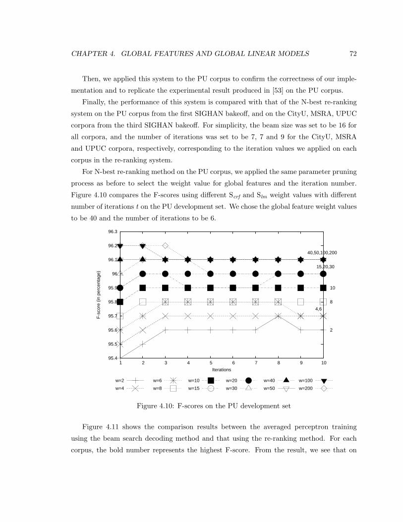
CHAPTER 4. GLOBAL FEATURES AND GLOBAL LINEAR MODELS 72
Then, we applied this system to the PU corpus to confirm the correctness of our imple-
mentation and to replicate the experimental result produced in [53] on the PU corpus.
Finally, the performance of this system is compared with that of the N-best re-ranking
system on the PU corpus from the first SIGHAN bakeoff, and on the CityU, MSRA, UPUC
corpora from the third SIGHAN bakeoff. For simplicity, the beam size was set to be 16 for
all corpora, and the number of iterations was set to be 7, 7 and 9 for the CityU, MSRA
and UPUC corpora, respectively, corresponding to the iteration values we applied on each
corpus in the re-ranking system.
For N-best re-ranking method on the PU corpus, we applied the same parameter pruning
process as before to select the weight value for global features and the iteration number.
Figure 4.10 compares the F-scores using different Scrf and Slm weight values with different
number of iterations t on the PU development set. We chose the global feature weight values
to be 40 and the number of iterations to be 6.
95.4
95.5
95.6
95.7
95.8
95.9
96
96.1
96.2
96.3
1 2 3 4 5 6 7 8 9 10
F-s
core
(in
per
cent
age)
Iterations
2
4,6
8
10
15,20,30
40,50,100,200
w=2
w=4
w=6
w=8
w=10
w=15
w=20
w=30
w=40
w=50
w=100
w=200
Figure 4.10: F-scores on the PU development set
Figure 4.11 shows the comparison results between the averaged perceptron training
using the beam search decoding method and that using the re-ranking method. For each
corpus, the bold number represents the highest F-score. From the result, we see that on

CHAPTER 4. GLOBAL FEATURES AND GLOBAL LINEAR MODELS 73
Corpus Setting F P R RIV ROOV
PU
Averaged perceptron with beam searchdecoding
94.1 94.5 93.6 69.3 95.1
Averaged perceptron with re-ranking,containing global and local features
93.1 93.9 92.3 94.2 61.8
Averaged perceptron with re-ranking,containing only local features
92.2 92.8 91.7 93.4 62.3
CityU
Averaged perceptron with beam searchdecoding
96.8 96.8 96.8 97.6 77.8
Averaged perceptron with re-ranking,containing global and local features
97.1 97.1 97.1 97.9 78.3
Averaged perceptron with re-ranking,containing only local features
96.7 96.7 96.6 97.5 77.4
MSRA
Averaged perceptron with beam searchdecoding
95.8 96.0 95.6 96.6 66.2
Averaged perceptron with re-ranking,containing global and local features
95.8 95.9 95.7 96.9 62.0
Averaged perceptron with re-ranking,containing only local features
95.5 95.6 95.3 96.3 65.4
UPUC
Averaged perceptron with beam searchdecoding
92.6 92.0 93.3 95.8 67.3
Averaged perceptron with re-ranking,containing global and local features
93.1 92.5 93.8 96.1 69.4
Averaged perceptron with re-ranking,containing only local features
92.5 91.8 93.1 95.5 68.8
Table 4.13: Performance (in percentage) Comparison between the averaged perceptron train-ing using beam search decoding method and that using re-ranking method
the CityU, MSRA and UPUC corpora, although the beam search decoding based system
still outperforms the re-ranking based system using only local features, the re-ranking based
system containing global features performs as good as or even better than the beam search
decoding based system. Therefore, it confirms again that global features have great influence
on performance in most cases.
On the other hand, for the PU corpus from the first SIGHAN bakeoff, the re-ranking
based method has worse performance than the beam search decoding based one. To explore
the rationale behind this phenomena, for each of the CityU, MSRA, UPUC, and PU test
sets, we examine how many sentences in the gold standard also appear within the 20-best
candidate list. Table 4.14 shows the corresponding ratios. From this table, we find that

CHAPTER 4. GLOBAL FEATURES AND GLOBAL LINEAR MODELS 74
92
93
94
95
96
97
98
PU CityU MSRA UPUC
F-sc
ore
(in p
erce
ntag
e)
Averaged Perceptronwith beam searchdecoding
Averaged Perceptronwith re-ranking,conaining global andlocal features
Averaged Perceptronwith re-ranking,conaining only localfeatures
Figure 4.11: Comparison for F-scores between the averaged perceptron training using beamsearch decoding method and that using re-ranking method, with histogram representation
CityU MSRA UPUC PURatio 88.2% 88.3% 68.4% 54.8%
Table 4.14: The ratio from examining how many sentences in the gold standard also appearwithin the 20-best candidate list, for the CityU, MSRA, UPUC, and PU test sets
for the PU test set, almost half of the true segmentations are not seen in the 20-best list,
which seriously affects the re-ranking process to pick up the correct candidate. While for the
CityU and MSRA corpora, nearly 90% of the gold standard appear in the 20-best candidate
lists, which provide better chances for the correct candidates to be picked up. Thus, in
order for the re-ranking method to have high performance, the quality of its candidate list
is extremely important. In comparison, for the beam search decoding based method, the
process of incremental character concatenation can produce more candidates to be examined,
without limiting itself to certain pre-defined 20-best candidates.

CHAPTER 4. GLOBAL FEATURES AND GLOBAL LINEAR MODELS 75
4.6 Exponentiated Gradient Algorithm
In the next experiment, we implement the batch exponentiated gradient (EG) algorithm
(see Figure 2.14) containing those two global features, explore the convergence for primal
(Equation 2.7) and dual (Equation 2.8) objective functions, and compare the performance
with the perceptron learning method, on the UPUC corpus.
In implementing the batch EG algorithm, during the initialization phase, the initial
values of αi,y are set to be 1/(number of N-best candidates for xi). Also, in the dual
variable update stage, considering Equation 2.6
α′i,y ←
αi,yeη∇i,y
Py αi,yeη∇i,y
where
∇i,y =
{0 for y = yi
1−Mi,y for y 6= yi
In order to get α′i,y, we need to calculate eη∇i,y . When each ∇ in the N-best list is positively
or negatively too large, numerical underflow occurs. To avoid this problem, ∇ is normalized,
and the above equation is modified to become
α′i,y ←
αi,yeη∇i,y/
Py |∇i,y |∑
y αi,yeη∇i,y/
Py |∇i,y |
(4.1)
in our implementation.
As before, the weight for global features is pre-determined using the development set
and is fixed during the learning process. Taking the difference on learning efficiency between
online update for perceptron learning and batch update for EG method into consideration,
the maximum number of iterations is set to be larger (T = 25) in the latter case during
parameter pruning. The weight for the global features are tested with 2, 5, 10, 30, 50,
70, and 90. Figure 4.12 shows the performance on the UPUC held-out set with various
parameters.
The experimental result tells us that, initially, as the number of iteration increases, the
F-score produced by EG method increases as well. However, larger numbers of iterations
could introduce over-fitting, causing the F-score to drop. In addition, the figure shows that
a larger weight for the global features produces better segmentation result. Therefore, we
select the number of iterations to be 22 and the weight for global features to be 90, and

CHAPTER 4. GLOBAL FEATURES AND GLOBAL LINEAR MODELS 76
91.5
92
92.5
93
93.5
94
94.5
95
95.5
96
1 2 3 4 5 6 7 8 9 10 11 12 13 14 15 16 17 18 19 20 21 22 23 24 25
F-s
core
(in
per
cent
age)
Iterations
25
10
3050,70,90
w=30 w=5 w=50 w=2 w=10 w=70 w=90
Figure 4.12: F-scores on the UPUC development set for EG algorithm
apply these parameters on the UPUC test set. Table 4.15 lists the resulting performance. In
this table, not only do we show the performance produced by the EG method using global
features, but also we list the performance from the EG method with only local features and
that from perceptron learning methods. Moreover, performance of the EG method with the
same number of iterations (t = 9) as the averaged perceptron method and that from the
character-based CRF method are listed as well. The bold number represents the highest
F-score.
From Table 4.15 and Figure 4.13, we see that the averaged perceptron with global
features still gives the highest F-score. Although the EG algorithm with global features
has better performance than the character-based CRF method, it takes more iterations in
achieving that result, and also it still performs worse than the averaged perceptron with
global features.
Continuing to run the EG algorithm for more iterations (T = 120) with the weight
of global features being fixed at 90, Figure 4.14 gives us the changes in primal and dual
objective functions. From the figure, we can see that the algorithm does in fact converge
to the maximum margin solution on this data set. However at iteration 120, the F-score

CHAPTER 4. GLOBAL FEATURES AND GLOBAL LINEAR MODELS 77
Setting F P R RIV ROOV
EG algorithm with global and local features 93.0 92.3 93.7 96.1 68.2EG algorithm with only local features 90.4 90.6 90.2 92.2 69.7EG algorithm with global and local features,with number of iterations being 9
92.4 91.7 93.1 95.5 67.6
Averaged Perceptron with global and localfeatures
93.1 92.5 93.8 96.1 69.4
Averaged Perceptron with only local fea-tures
92.5 91.8 93.1 95.5 68.8
Character-based CRF method 92.8 92.2 93.3 95.5 70.9
Table 4.15: Performance (in percentage) from the EG algorithms, comparing with thosefrom the perceptron learning methods and the character-based CRF method
90
90.5
91
91.5
92
92.5
93
93.5
F-sc
ore
(in p
erce
ntag
e)
EG algorithm with global andlocal features
EG algorithm with only localfeatures
EG algorithm with global andlocal features, with number ofiterations being 9
Averaged Perceptron with globaland local features
Averaged Perceptron with onlylocal features
Character-based CRF method
Figure 4.13: Comparison for F-scores from the EG algorithms, with those from the percep-tron learning methods and the character-based CRF method, using histogram representation

CHAPTER 4. GLOBAL FEATURES AND GLOBAL LINEAR MODELS 78
remains 0.930, which is the same as the F-score produced in the 22nd iteration.
-2.5e+06
-2e+06
-1.5e+06
-1e+06
-500000
0
500000
1e+06
1.5e+06
2e+06
2.5e+06
0 20 40 60 80 100 120
Iterations
Primal Objective Dual Objective
Figure 4.14: EG algorithm convergence on the UPUC corpus
4.7 Related Work
Re-ranking over N-best lists has been applied to so many tasks in natural language that it is
not possible to list them all here. Closest to our approach is the work done by Kazama and
Torisawa [19], for named entity recognition (NER). They proposed a max-margin perceptron
algorithm that exploited non-local features on an N-best list. Instead of using averaged
perceptron, their method for NER tries to maximize the margin between the best scoring
candidate and the second best scoring candidate, applying the original perceptron algorithm
with local features and non-local features that are defined on partial sentences. In contrast,
the averaged perceptron algorithm is used in our system, and global features are used to
examine the entire sentence instead of partial phrases. For word segmentation, Wang and
Shi [46] implemented a re-ranking method with POS tagging features. In their approach,
character-based CRF model produces the N-best list for each test sentence. The Penn

CHAPTER 4. GLOBAL FEATURES AND GLOBAL LINEAR MODELS 79
Chinese TreeBank is used to train a POS tagger, which is used in re-ranking. However, the
POS tags are used as local and not global features. Note that our experiments focus on the
closed track, so we cannot use POS tags. In machine translation, Shen et al. [38] investigated
the use of perceptron-based re-ranking algorithm, looking for parallel hyper-planes splitting
the top r translations and the bottom k translations of the N-best translations for each
sentence, where r + k ≤ n, instead of separating the one-best candidate with the rest. Also
in the tagging task, Huang et al. [18] modified Collins’ re-ranking algorithm [6], utilizing
n-gram features, morphological features and dependency features, for the Mandarin POS
tagging task.
4.8 Summary of the Chapter
In this chapter, we described our system for training a perceptron with global and local
features for Chinese word segmentation. We have shown that by combining global features
with local features, the averaged perceptron learning algorithm based on re-ranking pro-
duces significantly improved results, compared with the algorithm only using local features
and the character-based one-best conditional random field method. Also, we attempted to
automatically learn weights for global features. In addition, by comparing our system with
the beam search decoding based perceptron learning, we show again that global features are
useful. Moreover, the performance of the perceptron training is compared with that of the
exponentiated gradient method. We show that the averaged perceptron with global features
gives higher performance.

Chapter 5
Conclusion
In this thesis, we looked at the Chinese word segmentation problem, and reviewed various
common approaches applied in the literature. Also, we provided and evaluated two specific
Chinese word segmentation systems. This final chapter summarizes the contents of the
thesis in Section 5.1, re-emphasizes the contributions of our proposed approaches in Section
5.2, and points out certain possibilities for future work in Section 5.3.
5.1 Thesis Summary
In Chapter 2, various approaches dealing with Chinese word segmentation were described.
We classified these approaches into three main categories: the dictionary-based matching
approach, the character-based or subword-based sequence learning approach, and the global
linear model approach. Each of these categories, together with certain specific algorithms,
were explained in detail.
Chapter 3 described a character-level majority voting Chinese word segmentation sys-
tem, which voted among the initial outputs from the greedy longest matching, from the
CRF model with maximum subword-based tagging, and from the CRF model with min-
imum subword-based tagging. In addition, we experimented with various steps in post-
processing which effectively improved the overall performance. Moreover, a related voting
system, replacing the minimum subword-based CRF model with the character-based CRF
model during the majority voting, was described and compared.
Chapter 4 proposed the use of two global features, the sentence confidence score global
feature and the sentence language model score global feature, to assist with local features
80

CHAPTER 5. CONCLUSION 81
in training an averaged perceptron on N-best candidates for Chinese word segmentation.
We performed extensive experiments to compare the performance achieved from our system
with that achieved from the character-based CRF tagger, and also with that achieved from
perceptron learning using only local features. In addition, the beam search decoding algo-
rithm and the exponentiated gradient algorithm were implemented and compared with our
averaged perceptron learning system.
5.2 Contribution
The main contributions of this thesis in general are as follows:
• We show that the majority voting approach helps improve the segmentation perfor-
mance over its individual algorithms. The voting procedure successfully combines the
dictionary information used in the greedy longest matching algorithm and in the max-
imum subword-based CRF model, and thus raises the low in-vocabulary recall rate
produced by the two CRF-based discriminative learning algorithms. Also, the voting
procedure benefits from the high out-of-vocabulary recall rate achieved from these two
CRF-based algorithms. Thus, our majority voting system raises the performance of
each individual algorithms.
• We discover that by combining global features with local features, the averaged percep-
tron learning algorithm based on re-ranking produces significantly improved results,
compared to the character-based one-best CRF algorithm and the averaged perceptron
algorithm with only local features.
5.3 Future Research
There are many aspects of Chinese word segmentation that need to be further explored. For
instance, how should we effectively solve the unknown word problem, or at least what new
strategies could help to minimize its negative consequence and thus produces a significantly
higher out-of-vocabulary recall rate?
Also, in our perceptron training system, only two global features, the sentence confidence
score and the sentence language model score, are considered. Are there any other meaningful
global features that can also be included? In the future, we would like to explore more global

CHAPTER 5. CONCLUSION 82
features that are useful for perceptron learning. Also, the weight for the global features are
pre-determined and fixed in our system. Although we tried to update the weight for these
features during the learning process, the experimental accuracies were not encouraging.
Finding better methods for updating weights for the global features so that the perceptron
learning process can be done without a development set is an important topic for future
work.
In addition, during beam search based perceptron learning, only local features are in-
cluded. The language model score, as one of the global features, is able to provide additional
information about partial sentence candidates, and can be computed through the use of a
language model (e.g. use SRILM to score the partial sentence). In our experiments, we
attempted to involve the language model score feature in the beam search decoder: First,
SRILM is set up on the server side; then, the word segmentation system with beam search
decoder is run on the client side. For each sentence, after combining the next character
with all candidates up until the current character, the updated candidate list is sent to the
server, producing the language model score for each candidate, and then these language
model scores are sent back to the client system; After combining the language model fea-
ture score with other local feature scores, the top B best candidates in the list, where B
is the beam size, are retained and carried on to the next step. During the whole process,
the weight for the language model score feature is selected using the development set and
is fixed afterward. However, due to the delay caused by client-server communication and
the time spent on the calculation of language model score for each candidate, the running
speed is extremely slow. Also, the exhaustive weight determination for the global feature on
development set takes long time to complete as well. Thus, we have to regrettably abandon
this experiment and try to find a faster way to proceed. Effectively using not only the
language model score feature but also other global features inside beam search decoding
and then comparing its performance with other methods is an interesting experiment that
we leave for future work.

Bibliography
[1] Indrajit Bhattacharya, Lise Getoor, and Yoshua Bengio. Unsupervised sense disam-biguation using bilingual probabilistic models. In Proceedings of the 42nd Meeting ofthe Association for Computational Linguistics (ACL’04), Main Volume, pages 287–294,Barcelona, Spain, July 2004.
[2] Rich Caruana and Alexandru Niculescu-Mizil. An empirical comparison of supervisedlearning algorithms using different performance metrics. Technical Report TR2005-1973, Cornell University, 2005.
[3] Keh-Jiann Chen and Shing-Huan Liu. Word identification for mandarin chinese sen-tences. In Proceedings of the 14th conference on Computational linguistics, pages 101–107, Morristown, NJ, USA, 1992. Association for Computational Linguistics.
[4] Wenliang Chen, Yujie Zhang, and Hitoshi Isahara. Chinese named entity recognitionwith conditional random fields. In Proceedings of the Fifth SIGHAN Workshop onChinese Language Processing, pages 118–121, Sydney, Australia, July 2006. Associationfor Computational Linguistics.
[5] Shiren Ye Tat-Seng Chua and Liu Jimin. An agent-based approach to chinese named en-tity recognition. In Proceedings of the 19th international conference on Computationallinguistics, pages 1–7, Morristown, NJ, USA, 2002. Association for Computational Lin-guistics.
[6] Michael Collins. Discriminative reranking for natural language parsing. In Proc. 17thInternational Conf. on Machine Learning, pages 175–182. Morgan Kaufmann, SanFrancisco, CA, 2000.
[7] Michael Collins. Discriminative training methods for hidden markov models: Theoryand experiments with perceptron algorithms. In Proceedings of the Empirical Methodsin Natural Language Processing (EMNLP). MACL, pages 1–8, Philadelphia, PA, USA,July 2002. Association for Computational Linguistics.
[8] Michael Collins. Ranking algorithms for named entity extraction: Boosting and thevoted perceptron. In Proceedings of ACL 2002, pages 489–496, Philadelphia, PA, USA,July 2002. Association for Computational Linguistics.
83

BIBLIOGRAPHY 84
[9] Michael Collins. Parameter estimation for statistical parsing models: theory and prac-tice of distribution-free methods. pages 19–55, 2004.
[10] Michael Collins and Brian Roark. Incremental parsing with the perceptron algorithm.In Proceedings of the 42nd Meeting of the Association for Computational Linguistics(ACL’04), Main Volume, pages 111–118, Barcelona, Spain, July 2004.
[11] Aron Culotta, Andrew McCallum, and Jonathan Betz. Integrating probabilistic extrac-tion models and data mining to discover relations and patterns in text. In Proceedingsof the Human Language Technology Conference of the NAACL, Main Conference, pages296–303, New York City, USA, June 2006. Association for Computational Linguistics.
[12] Thomas Emerson. The second international chinese word segmentation bakeoff. InProceedings of the Fourth SIGHAN Workshop on Chinese Language Processing, pages123–133, Jeju Island, Korea, October 2005. Asian Federation of Natural LanguageProcessing.
[13] Yoav Freund and Robert E. Schapire. Large margin classification using the perceptronalgorithm. Mach. Learn., 37(3):277–296, 1999.
[14] L. Gillick and Stephen Cox. Some statistical issues in the comparison of speech recog-nition algorithms. In Proc. of IEEE Conf. on Acoustics, Speech and Sig. Proc., pages532–535, Glasgow, Scotland, May 1989.
[15] Amir Globerson, Terry Y. Koo, Xavier Carreras, and Michael Collins. Exponentiatedgradient algorithms for log-linear structured prediction. In ICML ’07: Proceedings ofthe 24th international conference on Machine learning, pages 305–312, New York, NY,USA, 2007. ACM.
[16] Simon I. Hill and Robert C. Williamson. Convergence of exponentiated gradient algo-rithms. In IEEE Trans. Signal Processing, volume 49, pages 1208–1215, June 2001.
[17] Julia Hockenmaier and Mark Steedman. Generative models for statistical parsing withcombinatory categorial grammar. In Proceedings of the 40th Annual Meeting of theAssociation for Computational Linguistics (ACL), pages 335–342, Philadelphia, USA,July 2002. Association for Computational Linguistics.
[18] Zhongqiang Huang, Mary Harper, and Wen Wang. Mandarin part-of-speech taggingand discriminative reranking. In Proceedings of the 2007 Joint Conference on Em-pirical Methods in Natural Language Processing and Computational Natural LanguageLearning (EMNLP-CoNLL), pages 1093–1102.
[19] Jun’ichi Kazama and Kentaro Torisawa. A new perceptron algorithm for sequencelabeling with non-local features. In Proceedings of the 2007 Joint Conference on Em-pirical Methods in Natural Language Processing and Computational Natural LanguageLearning (EMNLP-CoNLL), pages 315–324.

BIBLIOGRAPHY 85
[20] Balazs Kegl and Guy Lapalme, editors. Advances in Artificial Intelligence, 18th Con-ference of the Canadian Society for Computational Studies of Intelligence, CanadianAI 2005, Victoria, Canada, May 9-11, 2005, Proceedings, volume 3501 of Lecture Notesin Computer Science. Springer, 2005.
[21] Kyungduk Kim, Yu Song, and Gary Geunbae Lee. POSBIOTM/W: A developmentworkbench for machine learning oriented biomedical text mining system. In Proceedingsof HLT/EMNLP 2005 Interactive Demonstrations, pages 36–37, Vancouver, BritishColumbia, Canada, October 2005. Association for Computational Linguistics.
[22] Jyrki Kivinen and Manfred Warmuth. Exponentiated gradient versus gradient descentfor linear predictors. Technical Report UCSC-CRL-94-16, UC Santa Cruz, 1994.
[23] Taku Kudo, Yamamoto Kaoru, and Matsumoto Yuji. Applying conditional randomfields to japanese morphological analysis. In Dekang Lin and Dekai Wu, editors, Pro-ceedings of EMNLP 2004, pages 230–237, Barcelona, Spain, July 2004. Association forComputational Linguistics.
[24] John Lafferty, Andrew McCallum, and Fernando Pereira. Conditional random fields:Probabilistic models for segmenting and labeling sequence data. In Proc. 18th Interna-tional Conf. on Machine Learning, pages 282–289. Morgan Kaufmann, San Francisco,CA, 2001.
[25] Gina-Anne Levow. The third international chinese language processing bakeoff: Wordsegmentation and named entity recognition. In Proceedings of the Fifth SIGHAN Work-shop on Chinese Language Processing, pages 108–117, Sydney, Australia, July 2006.Association for Computational Linguistics.
[26] P. Liang. Semi-supervised learning for natural language. Master’s thesis, MassachusettsInstitute of Technology, 2005.
[27] Yuan Liu, Qiang Tan, and Xukun Shen. Chinese national standard gb13715: Contem-porary chinese word segmentation standard used for information processing. In Infor-mation Processing with Contemporary Mandarin Chinese Word Segmentation Standardand Automatic Segmentation Method. Tsinghua University Press, 1994.
[28] Albert Novikoff. On convergence proofs on perceptrons. In Proceedings of the Sym-posium on Mathematical Theory of Automata, pages 615–622. Polytechnic Institute ofBrooklyn, 1962.
[29] Constantine P. Papageorgiou. Japanese word segmentation by hidden markov model. InHLT ’94: Proceedings of the workshop on Human Language Technology, pages 283–288,Morristown, NJ, USA, 1994. Association for Computational Linguistics.
[30] Fuchun Peng, Fangfang Feng, and Andrew McCallum. Chinese segmentation and newword detection using conditional random fields. In Proceedings of Coling 2004, pages562–568, Geneva, Switzerland, August 2004.

BIBLIOGRAPHY 86
[31] Stephen Della Pietra, Vincent Della Pietra, and John Lafferty. Inducing features ofrandom fields. IEEE Transactions on Pattern Analysis and Machine Intelligence,19(4):380–393, 1997.
[32] Lawrence R. Rabiner. A tutorial on hidden markov models and selected applicationsinspeech recognition. In Proceedings of the IEEE, volume 77, pages 257–286. Instituteof Electrical and Electronics Engineers, Feburary 1989.
[33] Adwait Ratnaparkhi. A maximum entropy model for part-of-speech tagging. In EricBrill and Kenneth Church, editors, Proceedings of the Conference on Empirical Methodsin Natural Language Processing, pages 133–142, Somerset, New Jersey, 1996. Associa-tion for Computational Linguistics.
[34] Frank Rosenblatt. The perception: a probabilistic model for information storage andorganization in the brain. 65(6):386–408, 1958.
[35] Erik F. Tjong Kim Sang and Jorn Veenstra. Representing text chunks. In Proceedings ofEACL 1999, pages 173–179, Bergen, Norway, June 1999. Association for ComputationalLinguistics.
[36] Fei Sha and Fernando Pereira. Shallow parsing with conditional random fields. InNAACL ’03: Proceedings of the 2003 Conference of the North American Chapter ofthe Association for Computational Linguistics on Human Language Technology, pages134–141, Morristown, NJ, USA, 2003. Association for Computational Linguistics.
[37] Hong Shen and Anoop Sarkar. Voting between multiple data representations for textchunking. In Kegl and Lapalme [20], pages 389–400.
[38] Libin Shen, Anoop Sarkar, and Franz Josef Och. Discriminative reranking for ma-chine translation. In HLT-NAACL 2004: Main Proceedings, pages 177–184, Boston,Massachusetts, USA, May 2 - May 7 2004. Association for Computational Linguistics.
[39] Richard Sproat and Thomas Emerson. The first international chinese word segmenta-tion bakeoff. In Proceedings of the Second SIGHAN Workshop on Chinese LanguageProcessing, Sapporo, Japan, July 2003. Association for Computational Linguistics.
[40] Richard Sproat, William Gale, Chilin Shih, and Nancy Chang. A stochastic finite-stateword-segmentation algorithm for chinese. Comput. Linguist., 22(3):377–404, 1996.
[41] Andreas Stolcke. SRILM – an extensible language modeling toolkit. In Proceedings ofthe ICSLP, Denver, Colorado, 2002.
[42] Maosong Sun and Benjamin K T’sou. Ambiguity resolution in chinese word segmen-tation. In Proceedings of the 10th Pacific Asia Conference on Language, Informationand Computation, pages 121–126, Hong Kong, China, December 1995. City Universityof Hong Kong.

BIBLIOGRAPHY 87
[43] Charles Sutton and Andrew Mccallum. An introduction to conditional random fieldsfor relational learning. In Introduction to Statistical Relational Learning. MIT Press,2006.
[44] Cynthia Thompson, Siddharth Patwardhan, and Carolin Arnold. Generative models forsemantic role labeling. In Senseval-3: Third International Workshop on the Evaluationof Systems for the Semantic Analysis of Text, pages 235–238, Barcelona, Spain, July2004. Association for Computational Linguistics.
[45] Andrew J. Viterbi. Error bounds for convolutional codes and an asymptotically opti-mum decoding algorithm. In IEEE Transactions on Information Theory, volume 13,pages 260–269, April 1967.
[46] Mengqiu Wang and Yanxin Shi. Using part-of-speech reranking to improve chinese wordsegmentation. In Proceedings of the Fifth SIGHAN Workshop on Chinese LanguageProcessing, pages 205–208, Sydney, Australia, July 2006. Association for ComputationalLinguistics.
[47] Andi Wu. Customizable segmentation of morphologically derived words in chinese.Computational Linguistics and Chinese Language Processing, 8(1):1–27, 2003.
[48] Nianwen Xue. Chinese word segmentation as character tagging. Computational Lin-guistics and Chinese Language Processing, 8(1):29–48, 2003.
[49] Shiwen Yu, Huiming Duan, Bin Swen, and Bao-Bao Chang. Specification for corpusprocessing at peking university: Word segmentation, pos tagging and phonetic notation.Journal of Chinese Language and Computing, 13, 2003.
[50] Xiaofeng Yu, Marine Carpuat, and Dekai Wu. Boosting for chinese named entity recog-nition. In Proceedings of the Fifth SIGHAN Workshop on Chinese Language Processing,pages 150–153, Sydney, Australia, July 2006. Association for Computational Linguis-tics.
[51] Huipeng Zhang, Ting Liu, Jinshan Ma, and Xiantao Liu. Chinese word segmentationwith multiple postprocessors in HIT-IRLab. In Proceedings of the Fourth SIGHANWorkshop on Chinese Language Processing, pages 172–175, Jeju Island, Korea, Octber2005. Asian Federation of Natural Language Processing.
[52] Ruiqiang Zhang, Genichiro Kikui, and Eiichiro Sumita. Subword-based tagging byconditional random fields for chinese word segmentation. In Proceedings of the HumanLanguage Technology Conference of the NAACL, Companion Volume: Short Papers,pages 193–196, New York City, USA, June 2006. Association for Computational Lin-guistics.

BIBLIOGRAPHY 88
[53] Yue Zhang and Stephen Clark. Chinese segmentation with a word-based perceptronalgorithm. In Proceedings of the 45th Annual Meeting of the Association of Computa-tional Linguistics, pages 840–847, Prague, Czech Republic, June 2007. Association forComputational Linguistics.
[54] Hai Zhao, Chang-Ning Huang, and Mu Li. An improved chinese word segmentationsystem with conditional random field. In Proceedings of the Fifth SIGHAN Workshop onChinese Language Processing, pages 162–165, Sydney, Australia, July 2006. Associationfor Computational Linguistics.
[55] Junsheng Zhou, Liang He, Xinyu Dai, and Jiajun Chen. Chinese named entity recog-nition with a multi-phase model. In Proceedings of the Fifth SIGHAN Workshop onChinese Language Processing, pages 213–216, Sydney, Australia, July 2006. Associationfor Computational Linguistics.