1

Comparing Real Wage Rates†

By Orley Ashenfelter

A real wage rate is a nominal wage rate divided by the price of a good and is a transparent measure of how much of the good an hour of work buys. It provides an important indicator of the living standards of workers, and also of the productivity of workers. In this paper I set out the conceptual basis for such measures, provide some historical examples, and then provide my own preliminary analysis of a decade long project designed to measure the wages of workers doing the same job in over 60 countries—workers at McDonald’s restaurants. The results demonstrate that the wage rates of workers using the same skills and doing the same jobs differ by as much as 10 to 1, and that these gaps declined over the period 2000-2007, but with much less progress since the Great Recession. (JEL C81, C82, D24, J31, N30, O57)

I. Introduction

There is a long history of measuring, recording, and comparing real wage rates, dating at least from the Price Edicts of Diocletian in 301 AD.1 A nominal † Presidential Address delivered at the one hundred twenty-fourth meeting of the American Economic Association, January 7, 2012, Chicago, IL. Princeton University, Industrial Relations Section, Firestone Library, Princeton, NJ 08544 (e-mail: C6789@princeton.edu). I am deeply grateful to Stepan Jurajda of the Center for Economic Research and Graduate Education of the Charles University and the Economics Institute of the Czech Academy of Sciences; without his collaboration over the last decade this project would not have been possible. Martin Baily, then at the McKinsey Global institute, was invaluable in the start of the data collection for this project, while the staff at Pisacane GmbH have been invaluable since then. Ming Gu and Nicholas Lawson (at Princeton) and Peter Ondko (Prague) provided efficient assistance in the subsequent processing of the data. Financial support was provided initially with the assistance of the McKinsey Global Institute and subsequently by the Industrial Relations Section, Princeton University.1 Both Robert Allen (2007), who is a pioneer in such measurements, and Walter Scheidel (2009) have provided computations of Roman real wage rates and compared them with wage rates in other ancient times and places.

2

wage rate ($/hour) divided by the price of a good ($/good), is a transparent measure of how much of the good an hour of work buys (good/hour). As such, a real wage rate provides an important indicator of the living standards of workers. At the same time, the nominal wage rate is a also a measure of the price of labor, and when it is divided by the price of a good the worker produces it is a measure of how much of the good an hour of work produces. Thus, real wage rates are also connected to measures of labor productivity. This connection between wage rates, wellbeing, and productivity is at the heart of the modern economic analysis of labor markets.

In principle, properly constructed measures of the real wage would provide comparisons across places and over time, and their differences and movements would provide the opportunity to measure the effects of public policies and to test many types of economic models. Analyses that make use of real wages range from studies of economic growth and output accounting (Edward C. Prescott 1998, and Robert E. Hall and Charles I. Jones 1999), to international trade and finance (Jonathan Eaton and Samuel Kortum 2002, Daniel Trefler 1993, Kenneth Rogoff 1996), to the study of migration (Lutz Hendricks 2002, and Mark R. Rosenzweig 2010) and inequality (Angus Deaton 2010), and to problems of political economy (Dani Rodrik 1999).

Despite their obvious usefulness there is general agreement that the absence of comprehensive measures of real wage rates is one of the most serious gaps in our evolving system of economic measurement. One of the few efforts to remedy this situation was Richard B. Freeman and Remo H. Oostendorp’s (2000) attempt to standardize the data collected by the International Labor Organization (ILO). These October Inquiry data, collected since 1924, are provided by individual countries, but without any serious effort at standardization. As Freeman and Oostendorp (2000, p. 5) observe, “Recorded wages are not directly comparable across countries, in the same country over time, or even among occupations in a country at a point in time, in part because countries report data from differing national sources rather than conducting special surveys to answer

Diocletian’s efforts to stabilize wages and prices by edict in the 1st century apparently worked no better in the long run than similar attempts by others in the 20th century.

3

the ILO request.” Their conclusion? “…the Inquiry data has so many problems that the survey is one of the least widely used sources of cross-country data in the world.”

This situation stands in sharp contrast with the progress that has been made in comparing international prices through the International Comparison Project (ICP). The ICP was initially started by the United Nations Statistical Division with the University of Pennsylvania, but it is now housed in the World Bank. It seems apparent that it is far past the time when similar progress should be made in the measurement of wage data.

In this paper I provide some preliminary analysis of my own attempt to measure wage rates for comparable workers doing the same tasks in different places and at different times. My goal is to show just how useful a credible, transparent measure of the wage rate can be for economic analysis. The data I use come from an organization that is famous for producing the same product in different places and it has done so for many decades using a known production technology. The workers are thus using identical skills, using identical technology, and producing the same product. I am, of course speaking of workers at McDonald’s restaurants, and their famous product the Big Mac.

I begin by using some historical examples to show how important the measurement of real wages is for our understanding of economic progress. I then provide the basic economic analysis that underlies the conceptual apparatus for the measurement of real wages. This leads me to a summary exploration of the data on crew member wage rates at McDonalds (McWages) that I have collected over the last decade. The discussion proceeds in three parts. First, I provide some detail on how the data are collected and how they compare to the data for a more limited set of countries that we have available from the ILO and the US Bureau of Labor Statistics (BLS). Second, I provide summary measures by broad economic regions of the level of wage rates worldwide in 2007, a year I take to be normal by comparison with the period since. Finally, I explore the path that wage rates have taken in the normal period 2000-2007 and compare that with the path

4

they have taken since then in the aftermath of the world’s recent financial crisis, 2007-2011.

II. Historical Measures of Real Wages

Our long run conception of economic progress is based in our understanding of worker wages and welfare over long periods. For example, measuring worker welfare before, during, and after the industrial revolution sets the background for our understanding of the massive change in economic welfare that resulted. That, in turn, provides some perspective on how today’s developing countries may evolve in the future. In the last decade a lively set of analyses by economic historians has shed some new light on these old questions.

A. Before the Industrial Revolution

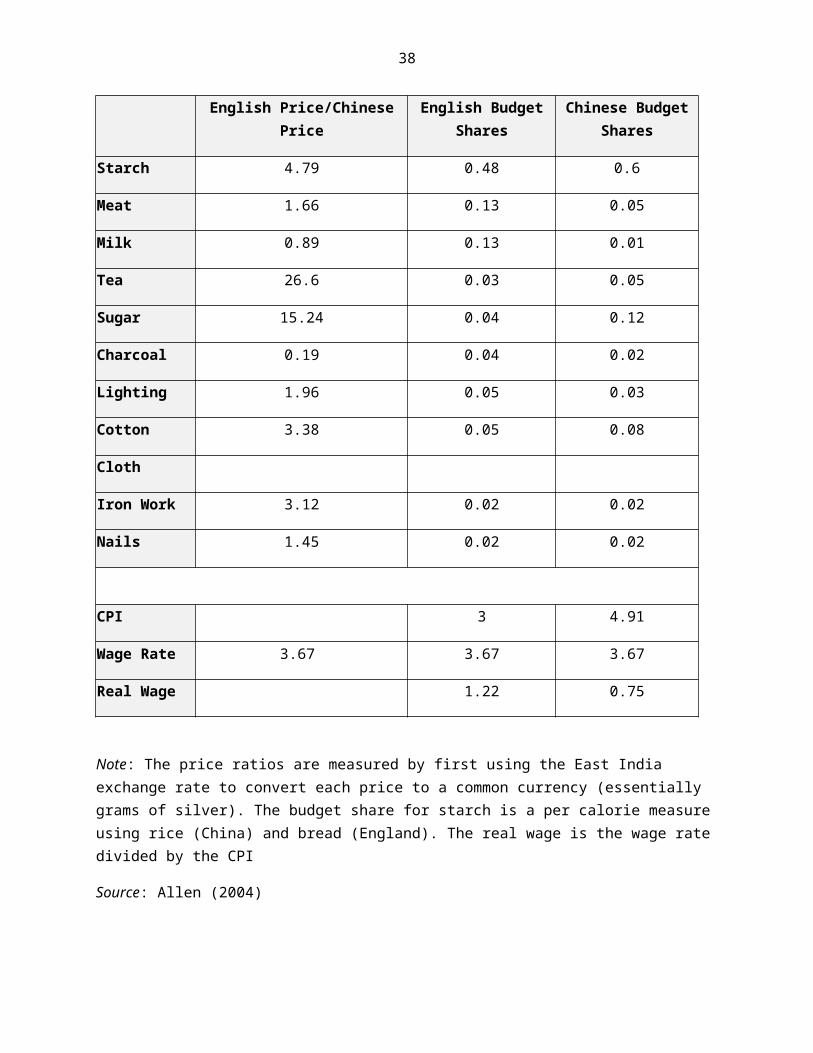
Table 1 provides an example of the problems of constructing real wage measures and also some perspective on an early period prior to the industrial revolution. Comparing wage rates between Canton Province in China and London in England in 1704 provides a benchmark for more modern comparisons.

The data for the calculations in the table are from the records of a member of the East India Company in the 18th century, and have been assembled by Robert Allen (2004). Wages and prices are measured using the East India Company exchange rates, which apparently closely mirror exchange rates measured in units of silver, a common currency in 1700. The results in Table 1 may come as a surprise to some.

First, as the first column of the table indicates, the nominal wage rate in London was between 3 and 4 times higher than in Canton. Second, it is also apparent from the table that nominal prices were generally, but not universally,

5

higher in London than in Canton. This, of course, suggests that real wage rates may not have been so different in the two places in 1704.

The second and third columns of Table 1 provide estimates of the budget shares for expenditures on various goods for both London and Canton, respectively. Using the English budget shares suggests that nominal prices were about 3 times higher in London than in Canton, while using the Chinese budget shares suggests that nominal prices were nearly 5 times higher in London than in Canton. This is an example of the classic index number problem, which in this case results from different budget shares in the two countries. From the point of view of a Cantonese, real wages are higher in Canton than in London because the work it would take to purchase a Cantonese lifestyle would be more in London than in Canton. Of course, precisely the opposite is the case from the point of view of a Londoner. An average of these two real wage measures, which is one version of an “ideal” index, implies that real wage rates were about the same in Canton and London before the industrial revolution in England.2

It is my impression that this finding about the broad uniformity of real wage rates across space in the period before the industrial revolution is slowly being confirmed as a key fact in the history of economic development. Perhaps this accounts for the broad pessimism of the classical economists about the prospect for long run growth in real wage rates.

B. Wage Rates During and After the Industrial Revolution

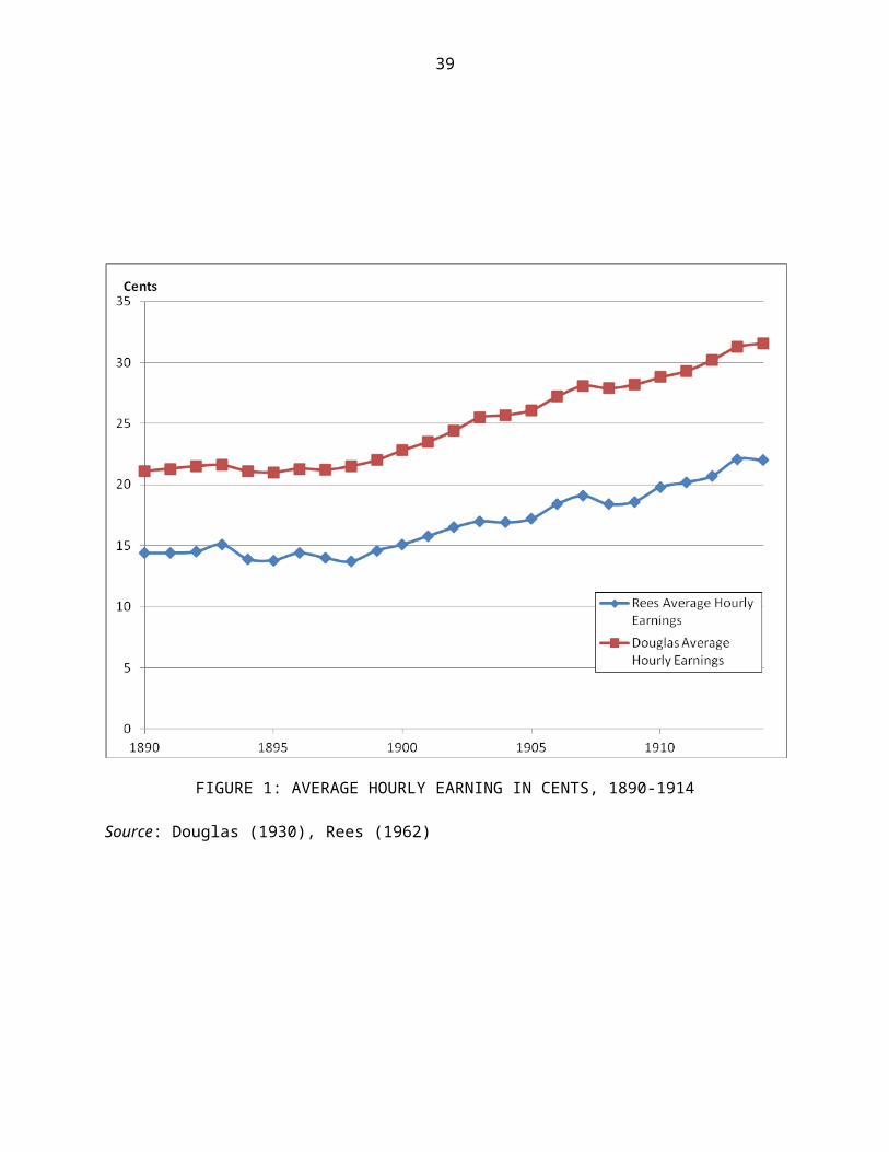
Paul Douglas (1930) painstakingly constructed estimates of real wage rates in manufacturing in the US from 1890-1914. Douglas’s results had the surprising implication that, even though output per man hour increased in this period of industrial growth, real wage rates did not. The Douglas series for nominal wage rates is displayed in Figure 1 along with an alternative series constructed many

2 This differs somewhat from Angus Maddison’s (1998) “guesstimate” that European gross national product per capita may have been about 50% higher than in China in 1700. Nevertheless all the evidence suggests that Chinese/European differences before the industrial revolution were not nearly as large as in the period after the industrial revolution, as in shown below in Table 2.

6

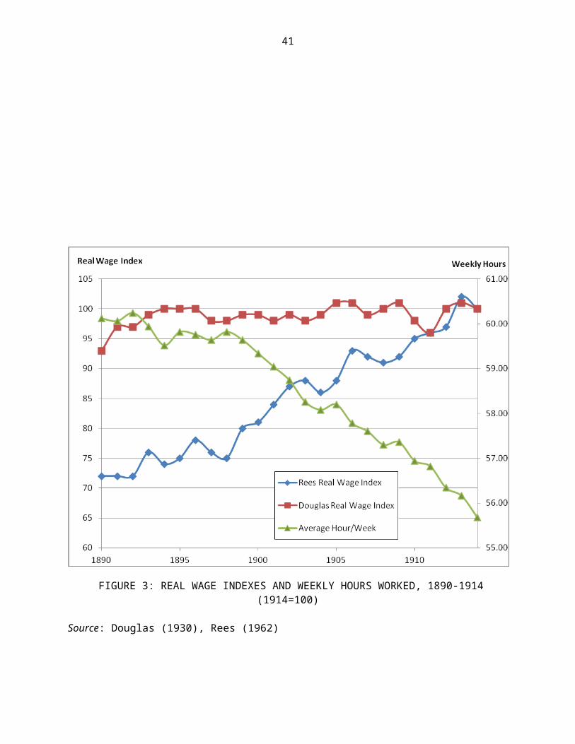
years later by Albert Rees (1961) when he revisited this puzzle. Douglas’s real wage index is displayed in Figure 3 and shows remarkable stability.

Rees speculated that (a) an increased labor supply, caused either by the closing of the American frontier and an increase in immigration, or (b) an increase in the return to capital might explain the puzzle. But the evidence from the growth in real wage rates in the period after 1914 seemed inconsistent with either explanation. An alternative possibility was that either the nominal wage or the price series had missed some change in the key facts.

Rees expanded his nominal wage series to provide increased coverage of non-union wage rates, which Douglas had used less extensively. The two series on nominal wage rates are shown in Figure 1 and differ in an expected direction, but their trend turned out to be no different.

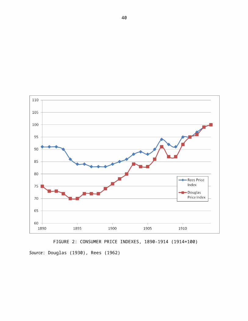
With respect to his new price index, Rees undertook a serious attempt to include data on the prices of manufactured consumer products, which had been difficult for Douglas to capture. Rees’s main innovation was the use of detailed prices and product descriptions from Sears and Roebuck and Montgomery Ward catalogs—these were something like the internet purchasing guides of their day.

Figure 2 compares Douglas’s and Rees’s nominal price series, and Figure 3 compares the resulting real wage indexes. It is apparent that, unlike Douglas’s series, Rees’s price index remains stable in the face of increasing nominal wage rates. Rees’s price series thus implies an increase in real wage rates that Douglas’s series did not. An important puzzle about real wage rates in the US during the industrial revolution was not much of a puzzle at all. The lesson from this analysis is that an investment in careful data appraisal can generate a large return in economic measurement.

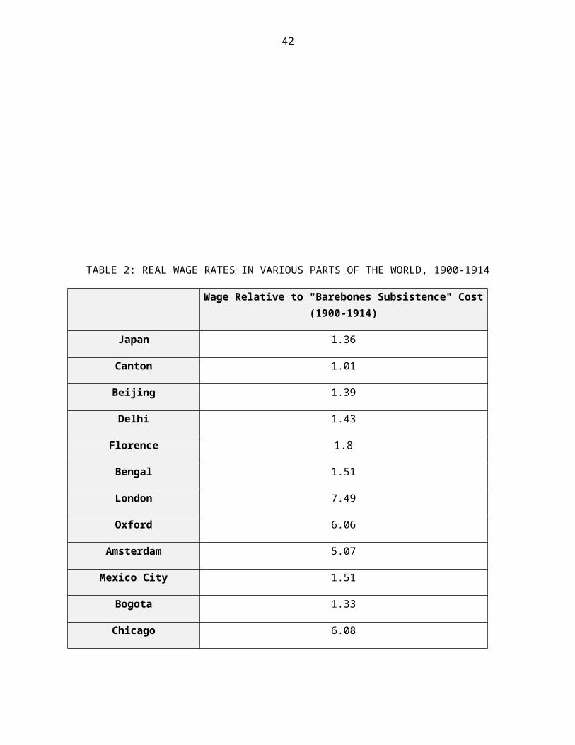
Finally, Table 2 provides some evidence comparing real wage rates in various parts of the world in 1914, the period when Rees concluded his measurement. In contrast with the data in Table 1, the data in Table 2 tell a remarkable story of a dramatic widening in the gap between wage rates in much of Europe and the US compared to wage rates in most of the rest of the world.

7

Real wage rates in London and Canton, which two centuries earlier had been nearly the same, had diverged dramatically. As Table 2 shows, over a period of a century or two economic growth had been so uneven that enormous gaps had opened up between what we now consider the rich and the poor countries, resulting in real wage rates that were 4 to 5 times higher in the rich countries. This raises the natural question of whether these gaps are likely to persist and, if they do not, how best to measure them as they close.

III. Conceptual Real Wage Measures

As Figure 3 indicates, sizeable changes in real wage rates have historically been accompanied by declines in normal hours of work. Indeed, the normal work week in US manufacturing in 1890 was based on a 10 hour day, six days a week for a total of 60 hours a week. By 1914 weekly hours had declined by about 7% in the face of a real wage rate increase of about 40%, implying that real earnings (the wage rate times hours of work) had increased by only one-third, considerably less than the 40% they would have increased if work hours had remained constant. Over longer periods of more dramatic real wage growth the contrast is even more striking. By 2007, for example, before the recent recession, weekly hours worked in US manufacturing were around 40. At current wage rates, weekly earnings would be 50% higher today than they actually are if work hours had not declined so dramatically since 1890. Clearly, a considerable part of the increase in the real hourly wage was used to reduce hours at work.3

As John Pencavel (1977) noted, the implication of a negatively sloped long run labor supply function is that observed earnings or income differences may be a misleading measure of welfare differences when wages rates differ dramatically. It follows that an appropriate measure of the real wage rate that is intended to measure welfare should be based on a model in which labor supply and commodity consumption are selected jointly by a consumer-worker.

A. Constant-Utility indexes of Real Wages3 An early analysis of long run labor supply, emphasizing this point, is H. Gregg Lewis (1957). There is also considerable evidence, at least since Gordon Winston (1966), that high wage countries have far shorter work weeks than low wage countries. This implies that comparisons of average earnings in rich and poor countries may also understate welfare differences.

8

In the conventional set up a consumer-worker maximizes utility u(l,c) subject to the budget constraint pc=wh+y, where c indicates consumption goods, w is the nominal wage rate, p is a set of prices of consumption goods, h=T-l is hours worked, l is non-work time, T is the total time endowment, and y is income unrelated to work. The usual first order conditions lead to a labor supply function h(w,p,y) and commodity demand functions ci = ci (w, p, y) and, after substitution, to the indirect utility function u(T-h(w,p,y),c(w,p,y))= v(w,p,y).

The solution of v(w,p,y) for w*=w*(p,y,v*) is the lowest wage rate that permits a consumer with non-work income, y, facing prices, p, to reach the reference utility level v*. The function w* provides the basis for a constant-utility index number of real wages. A comparison of the observed w with w* indicates whether the worker’s real wage has increased. w/w* is thus a real wage index from the worker’s point of view.

It is easy to show that w* is increasing in prices, p, as would be expected. But it is also easy to show that w* is decreasing in non-work income, y. In other words, the lowest wage rate that permits a worker to reach the reference utility level, v*, increases when prices increase, but it decreases when non-labor income increases. Approximating the effect of prices on w* raises all the usual problems of index number base levels (Deaton 2010) and purchasing power parity measurement.

An interesting insight from this formulation is that comparisons of real wage rates for economies where non-work income differs substantially may be seriously misleading. Wage rates in economies that provide economic safety nets, for example, may result in lower work effort, but real wage rates in such economies are higher than a simple price adjustment applied to the nominal wage would imply.

In most applications it is not possible to measure non-work income. Pencavel (1977) suggests simply assuming that non-work income does not differ in the different places or times where wage rates are being compared. Using this assumption, and estimates of the necessary parameters from Michael Abbott and Orley Ashenfelter (1976), Pencavel shows that the conventional measure of the

9

real wage index provides a workable approximation to the constant-utility real wage rate even when wage rates change substantially.

Another interesting feature of a constant-utility real wage index is that it provides a way to measure welfare differences that does not depend on any assumption about competition in product or labor markets, or about the absence of minimum or maximum wage regulations. Although product market monopoly or labor market monopsony reduces real wage rates, this is fully reflected in a lower real wage rate and a lower level of worker welfare. Likewise, a wage regulation that increases the real wage results in a higher level of worker welfare. On the other hand, the existence of quantity restrictions on work effort, such as unemployment, implies that the real wage alone is not a sufficient indicator of welfare differences.4

B. Real Wage as Marginal Product of Labor

At the same time as the real wage rate determines labor supply, it also plays a key role in the demand for labor. A profit maximizing firm treats the wage rate as the price of labor and hires workers to the point where the value of an additional worker’s marginal product is equal to it. The familiar relation Pmp=w, where P is output price and mp is the marginal product of labor, implies that w/P is a measure of the physical marginal product of labor when firms are maximizing profits and there are competitive labor and product markets. If follows that real wage rate differences can also be used to measure productivity differences under some circumstance.

To see how this can be done consider the typical Cobb-Douglas5 production function of growth accounting, written conveniently as Hall and Jones(1999) do to isolate total factor productivity (TFP), as

(1) yi=Ai (Ki/ Yi) α/(1- α) hi,

4 See Ashenfelter (1980) and Ham (1982) for an analysis when workers face quantity restrictions on the amount they may work at a given wage rate. 5 See Paul Douglas (1948). This is the same Douglas, of course, whose real wage series is contained in Figure 3.

10

where, for country or time period i, yi is output per worker, Ki/Yi is the capital/output ratio, hi is human capital per worker, Ai is TFP, and ɑ is the capital coefficient in the aggregate production function. Adjusting output per worker by a measure of human capital and the capital/output ratio then provides a direct measure of TFP. Capital/output ratios are typically taken as directly measured, and ɑ=1/3 is often assumed, which then leaves the question of how to measure the human capital of the work force in country or time period i. Various creative approaches to this measurement issue have been used. Hall and Jones (1999) and Jones and Romer (2010) assume that h can be represented by a Mincer-style earnings function and use estimated returns to schooling to construct measures of hi. Hendricks (2002) assumes that the wage of observationally equivalent workers who migrate from country i to work in the US, compared to the wage of workers from the US who work in the US, provides a measure of differences in hi.

Assuming workers are paid their marginal products implies that it is also possible to use the wage rates of workers doing identical jobs in different countries or at different times to account for human capital differences. A worker with the base skill level h0i will be paid w0i which, because marginal products are proportional to average products in a Cobb Douglas production function, will be proportional to Ai (Ki/ Yi) α/(1- α) h0i. Since h0i =h00 (for all i) for workers using the same skills, it follows that the wage rate of the base level skilled worker (w0i) in country i can be expressed, relative to the wage rate of the base level skilled worker in a base country (w00), using (1) as

(2) w0i/w00= [Ai (Ki/ Yi) α/(1- α)]/ A0 (K0/ Y0) α/(1- α).

According to (2), if workers are paid their marginal products, wage ratios of the base skill group can be accounted for by differences in capital/output ratios and differences in total factor productivity. Differences in human capital per worker will not affect this wage ratio because the workers being compared are using the same skills. Alternatively, equation (2) also implies that adjusting relative wages for differences in capital/output ratios will provide a measure of relative total factor productivity (Ai/A0). Of course, if the wage structure is distorted by minimum wages or monopoly or monopsony in product or factor markets, the

11

assumption that h0i is the same in each country will fail. Thus, assumptions about competitive markets are critical for using wage rates to measure TFP.

C. Product Prices and Real Wage Rates

If real wage rates differ from place to place, then the prices of non-tradable goods will also differ from place to place. Prices of non-tradables must differ because local wage rates indicate the cost of a factor of production that is important in producing a non-tradable good. These input price differences will thus result in output price differences. This point is very important for understanding what price deflator is appropriate for the computation of a real wage. The simplest version of this phenomenon, often known as the Balassa-Samuelson effect,6 is based on the observation that if tradable goods prices are the same everywhere, and if productivity differs in the production of tradable goods, then the prices of non-tradable goods must differ too. This results because the equality of wage rates between workers in the tradable and non-tradable sectors within a country makes labor intensive goods more expensive to produce in high productivity countries.

Consider a product produced according to a Cobb-Douglas production function from a combination of both tradable goods and local labor that is paid wage w0i. The cost of producing such a good will be

(3) pni=w0iap1-a,

where pni is the price of the quasi-tradable good, p is the (constant across places) price of tradable goods, and 0<a<1, is the fraction of the cost of production that is due to local labor. Equation (3) describes the price of the quasi-tradable good as a concave function of the local wage. A real wage defined as

(4) w0i/pni=(w0i/p)1-a,

is a purchasing-power-parity price adjusted wage, where the weights in the purchasing power basket are allocated in the proportion a and 1-a to non-tradables and tradables, respectively. This index is a concave function of the

6 See Balassa (1964) and Samuelson (1964).

12

wage rate measured in the tradable price and it will thus show a smaller gap between high and low wage countries than would a real wage rate measured in tradable prices. It is natural to think of the tradable-goods-based wage rate , w0i/p, as being measured by the wage rate expressed in a common currency, since exchange rates are meant to equate the prices of tradable goods. It is this wage rate that should be linked to the marginal product of labor and TFP. Likewise, it is natural to think of the quasi-tradable-goods-based wage rate, w0i/pni , as more closely related to the welfare of workers as represented by a constant-utility real wage index.

IV. Measuring McWages

To demonstrate how a well-defined real wage rate may be used, I have been collecting data on wages (and prices) from McDonald's restaurants since 1998. Perhaps the most famous statement of the identical nature of the items McDonald’s sells was articulated by Thomas Friedman (1999, p. 239) in his bestselling The Lexus and the Olive Tree: “Every once in a while when I am traveling abroad, I need to indulge in a burger and a bag of McDonald’s French fries. For all I know I have eaten McDonald’s burgers and fries in more countries of the world than anyone, and I can testify that they all really do taste the same (italics in the original).”7

A. Data Collection

There is a reason that McDonald’s products are similar. These restaurants operate with a standardized protocol for employee work. Food ingredients are delivered to the restaurants and stored in coolers and freezers. The ingredients and food preparation system are specifically designed to differ very little from place to place. Although the skills necessary to handle contracts with suppliers or to manage and select employees may differ among restaurants, the basic food preparation work in each restaurant is highly standardized. Operations are monitored using the 600-page Operations and Training Manual, which covers

7 Friedman goes on to use this observation to advance his controversial “Golden Arches Theory of Conflict,” which posits that countries with McDonald’s restaurants do not engage in warfare with each other.

13

every aspect of food preparation and includes precise time tables as well as color photographs.8

A key motivation for the use of standardized work protocols is the implied warrantee of food safety that eating at a McDonald’s restaurant provides when a traveler has little information about the quality of local establishments. The standardized McDonald’s brand is both a risk (in case of some failure) and a reward (when failure is rare). As a result of the standardization of both the product and the workers’ tasks, international comparisons of wages of McDonald’s crew members are free of interpretation problems stemming from differences in skill content or compensating wage differentials. I suspect there are other internationally diversified companies that have a similar structure and that might also make suitable candidates for data collection.

My original survey of McDonald’s wages was carried out as a pilot project with the cooperation of the McKinsey Global Institute. To determine if the project was feasible, data were collected in the month of December 1998 for a limited list of 13 countries.9 Since the data collection went quite smoothly the primary project was started with the collection of data for 27 countries during the summer of 2000, specifically including a number of transitional and developing countries.

In general, the data collection was for McDonald’s restaurants operating in a large urban area, typically a capitol city or, in larger countries, the two largest cites. In later work, starting in 2007, data were collected for this project with a business intelligence firm. For larger countries data were collected in multiple locations, stratified by city size. In most cases wage rates are simply hourly pay, without any adjustment for benefits or taxes. In some cases the data indicated a pay scale giving wage rates depending on seniority; in this case the mid-point of

8 A candid description of these procedures is provided by Royle (2000). About 90% of all employees at McDonald’s are hourly paid Crew and Training Squad workers. Employees typically start work at a food preparation station, and are then rotated through various stations and eventually to the sales counter. As a result, workers may undertake several different assignments at different times.

9 Belgium, Brazil, Czech Republic, France, Germany, Italy, Japan, Korea, Poland, Russia, Sweden, UK, and USA. Our concern was the reputation that McDonald’s has for secrecy regarding many of its practices.

14

that scale was taken as the wage rate. Finally, in a few countries it was necessary to estimate an hourly wage rate based on an average monthly salary divided by average hours worked.

Although the reliability of these data is hard to assess at a general level, there is quite a bit of anecdotal evidence to support the estimates shown below. It is straightforward to compare our estimates of Big Mac prices with those that the Economist magazine has reported for many years. The correlation averages about .99. Other evidence comes from personal data collection, often provided by economists who have eaten in a McDonald’s restaurant.

B. Comparisons to Other Wage Data

One direct way to assess the reliability of these data is to compare them to what other data already exist. Although McDonald’s currently operates in about 120 countries, many of these are very small. As of 2007, my data on wage rates in McDonald’s restaurants (the McWage) are available for about half of these countries. There are no other sources of wage data with such broad coverage, but there are several sources that provide more limited opportunities for comparison.

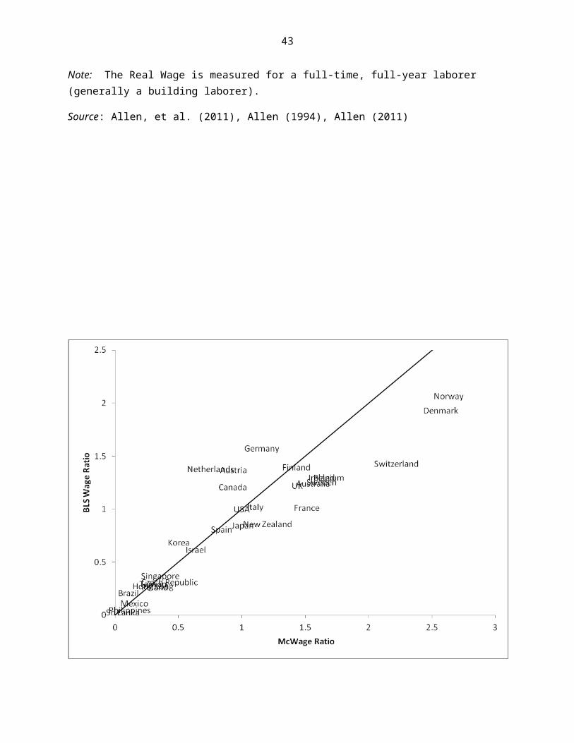
One of the best known sources for international comparisons of wage rates is that provided by the US Bureaus of Labor Statistics (BLS) for wage rates and compensation costs in manufacturing. Although the occupations covered are certainly not directly comparable, these BLS data nevertheless provide a general measure of the level of wage rates in the broad labor market in several countries. The result of a comparison of the McWage (converted to US dollars at then-current exchange rates) and the BLS wage measures (also in US dollars) for 2007 is contained in Figure 4.

In Figure 4 wage rates for each country are expressed relative to the US. Thus the point (1,1) represents the combination of the US McWage and the BLS wage measure for the US. The line drawn is a 45 degree line, so that points above it indicate a relative BLS wage higher than the comparable McWage, and points below it represent a relative BLS wage that is lower than the comparable

15

McWage. It is apparent from the figure that these two separate measures of the wage rate are closely related.

Two additional points are worth noting. First, no matter whether measured by the BLS data or the McWage, there are many countries that have higher, and in some cases far higher, wage rates than the US. Second, in the richer countries with a high minimum wage (as in Denmark), the McWage tends to be higher than the BLS measure of the wage. It follows that when minimum wages are binding on McDonald’s restaurant workers considerable care is required in the interpretation of the McWage.

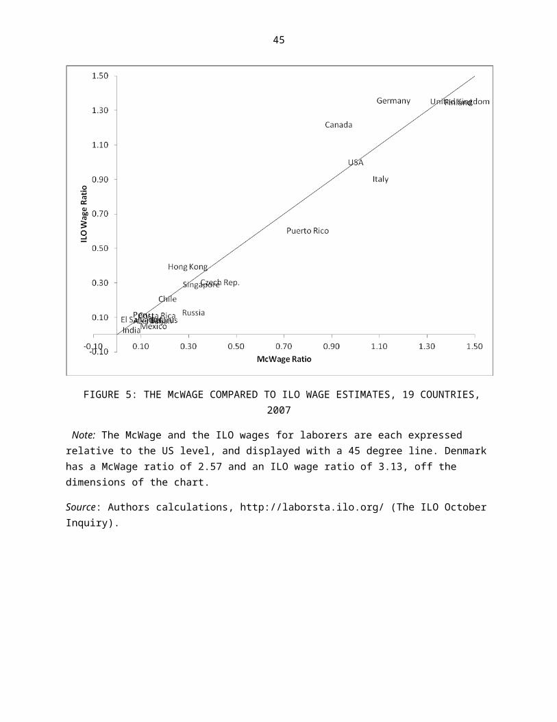
Figure 5 compares, using the same graphical method, the McWage and the wage rates for laborers from the available ILO data for 2007. As with the BLS data, it is apparent that both these measures of the wage rate are highly related. The ILO data contain more representation from very low wage countries than the BLS data and for these the McWage appears, if anything, to be higher than the laborer wage rate. This may, of course, represent differences in how a laborer’s occupation is defined in the different countries from which the ILO has obtained data.

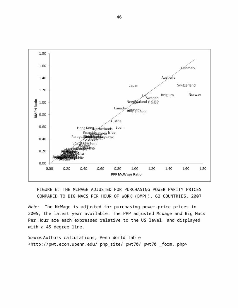
Figure 6 provides a comparison of the McWage deflated by two different price indexes. The data in Figures 4 and 5 refer to wages measured in a common currency, and they may therefore be considered as measured in the price of tradable commodities. These measure the cost in a common currency of employing a worker. By contrast, Figure 6 compares two measures that deflate the McWage by price indexes that may be thought to measure the prices a consumer-worker faces for a basket of goods (containing both tradable and non-tradable goods) that consumer-worker’s actually purchase.

The more common measure of a purchasing-power-price (PPP) index from the ICP is used to deflate the McWage on the horizontal axis of Figure 6. A more unconventional measure of purchasing power is used to deflate the McWage on the vertical axis: the price of a Big Mac. What is apparent from the comparison of the PPP-deflated McWage and the measure of Big Macs per Hour Worked (BMPH) is that they are very closely related.

16

The reason for this is apparent from Figure 7, which plots the Big Mac price against the US dollar measure of the McWage. The motivation for this plot is equation (3), which displays the same concave form as is displayed in the figure. Figure 7 has an eerie resemblance to the plot of PPP prices against real GDP per capita in Summers and Heston (1991), suggesting that both plots are reflecting the Balassa-Samuelson effect noted above. The regression estimate of the parameter a, which has the interpretation as the fraction of a Big Mac that is non-tradable and due to labor costs, is about .6.10

For the less developed countries there is a clear tendency for the PPP adjusted McWage to be greater that the BMPH in Figure 6. There are many possible interpretations of this, but one obvious possibility is that the Big Mac is a more expensive (i.e., tradable) bundle of goods than is appropriate for indexation of wage rates in very low wage countries. On the other hand, it is worth noting that the BMPH does not depend on any exchange rate adjustment, so that distortions in exchange rates do not affect its calculation.

Figure 8 provides a final comparison of McWages with output per man hour for countries where this is available. These variables are also highly correlated, but there is a very noticeable tendency for the McWage to be elevated relative to output per man hour in countries with high minimum wages. This is an important issue to consider when using wage rates to provide indirect measures of aggregate productivity.

V. Comparisons of the Level of Real Wages

Table 3 provides a basic cross-section of data for 2007 on prices and wages from McDonald’s restaurants. In order to create a manageable, readable table I have aggregated the more than 60 countries for which there are data into a group of economic regions. These are admittedly only a heuristic device for ease of interpretation, but the aggregation used here captures about 85% of the

10 This is not far from the fraction of the cost of a Big Mac that Parsley and Wei (2007) estimate as due to labor costs. Parsley and Wei also report a detailed study of the cost components of the Big Mac and their reaction to exchange rates.

17

variability in the raw data on wage rates.11 The year 2007 was selected both because the sample of countries for which data were collected was expanded in that year, but also because the financial crisis that affected many countries had not yet begun.

The first column of Table 3 contains the wage rate for a McDonald’s crew member in US dollars (at then-current exchange rates), while the third column contains the price of a Big Mac (again in US dollars). For ease of comparison the second column expresses the McWage in the economic region indicated relative to its value in the US. Finally, the fourth column contains the ratio of the price of a Big Mac to the McWage (that is, it contains the measure of Big Macs per hour of work, BMPH).

There are three obvious, dramatic conclusions that it is easy to draw from the comparison of wage rates in Table 3. First, the developed countries, including the US, Canada, Japan, and Western Europe have quite similar wage rates, whether measured in dollars or in BMPH. In these countries a worker earned between 2 and 3 Big Macs per hour of work, and with the exception of Western Europe with its highly regulated wage structure, earned around $7 an hour. A second conclusion is that the vast majority of workers, including those in India, China, Latin America, and the Middle East earned about 10% as much as the workers in developed countries, although the BMPH comparison increases this ratio to about 15%, as would any purchasing-power-price adjustment. Finally, workers in Russia, Eastern Europe, and South Africa face wage rates about 25 to 35% of those in the developed countries, although again the BMPH comparison increases this ratio somewhat. In sum, the data in Table 3 provide transparent and credible evidence that workers doing the same tasks and producing the same output using identical technologies are paid vastly different wage rates. As we shall see, a straightforward explanation of these vast wage differences attributes them almost entirely to differences in the total factor productivity in these countries, not to differences in skill or human capital.

11 That is, a regression of the McWage for all countries on dummy variables representing these regions explains about 85% of the variance in wage rates.

18

Table 4 shows measures of hypothetical total factor productivity for each economic region relative to the US. The first column of the table provides a measure of TFP using the method proposed by Hall and Jones (1999), but which I have updated to 2007 using the data in the Penn World Table 7.0. The Hall-Jones method is based on adjusting output per man for (a) differences in schooling levels of the work force and (b) capital/output ratios, but I have here assumed capital/output ratios are the same in all countries. The second column shows the results of using equation (2) to measure the hypothetical TFP with the relative wage of workers in McDonald’s restaurants.

It is apparent from Table 4 that for a vast part of the world the measures of TFP based on wage rates are remarkably similar to those based on output accounting measures. This is not surprising given the high correlation between the McWage data and output per man hour indicated in Figure 8 and the key role that output per man hour plays in the calculation of conventional TFP measures. Given the potential for error in these calculations, however, the similarity of these estimates is impressive, especially in view of the simplicity with which it is possible to estimate TFP from wage rate differences. Since the adjustment for capital/output ratios plays such a small role in these calculations (see Hall and Jones (1999), Table 1) it is apparent that McWage ratios are, by themselves, good short hand measures of TFP differences across countries.

Figure 9 displays the relation between the TFP measures contained in Table 4. This figure shows where the wage based measures of TFP are problematic. In countries with very high minimum wage rates, like Australia and much of Western Europe, the wage structure is altered and the McWage no longer serves as a measure of aggregate output differences.12 Monopoly in the product market or monopsony in the labor market would also undermine the usefulness of wage rates for this purpose.13

12 This does not necessarily mean that the marginal product of a worker in the sector covered by a minimum wage statute differs from the wage rate actually paid, but it does mean that the wage structure has been altered. The resulting distortion of relative wages means that the McWage does not serve as a way to measure differences in the overall level of wage rates in a country’s labor market.13 Without competitive labor and product markets the firm’s first order condition for profit maximization requires that marginal revenue product equal marginal factor cost. The former will generally be lower than the firm’s output price, and the latter will generally be greater than the wage rate, which means that in either case the real

19

VI. Comparing Changes in Real Wages

Table 5 and Figures 10, 11, and 12 provide details on wage and price changes over the period 2000-2007. Data were collected for a much more limited set of countries in the early part of this period, so that the number of comparisons is more limited for this period.

The first, third, and fourth columns of Table 5 provide the ratio of the McWage, the price of a Big Mac, and the BMPH in 2007 to the value in 2000. These ratios provide measures of growth. In the second column the growth in a country’s wage is expressed relative to the growth in the US-- a measure of the difference in growth from the US.

All these wage rates and prices are expressed in US dollars at then-current exchange rates. If exchange rates fully reflect changes in the prices of tradables, as the purchasing power parity hypothesis suggests, then these wage and price changes are fully comparable across countries. However, the purchasing power parity hypothesis, even if accurate for longer periods of time, may not be appropriate in the analysis of shorter periods.14 An attractive feature of the BMPH measure of the real wage rate is that it does not rely on exchange rates at all. It is a direct physical measure of the output a worker may purchase with an hour of work, and it is comparable over time and across space.

The primary message of Table 5 and the accompanying figures is that growth in real wage rates was entirely confined to the developing countries of Russia, India, and China during the period 2000-2007.

Generally speaking each country represented in Table 5 displays increases in nominal wages and prices. What is remarkable is the dramatic disparity in the growth in real wages as measured by the BMPH. In both Canada and the US the real wage rate declines somewhat, while in Japan it does not change.15 In

wage rate (measured in terms of the firm’s product price) is not equal to the marginal product of labor.14 See especially Rogoff (1996) for a useful survey of the issues.15 Unfortunately, data for some of the countries in the economic region defined as Western Europe in previous tables was not collected in 2000, so a broad comparison for this region over the period 2000 to 2007 is not possible. A more detailed analysis at the level of the country, rather than the region, would show a broadly similar conclusion, but with some growth in real wage rates in Eastern Europe.

20

contrast, the growth rate in real wages is over 50% in this period in China and India, while it is over 150% in Russia. The choice of 2000 for the start of data collection is unfortunate in the case of Russia, as it is well known that the Russian financial crisis in the late 1990s resulted in a collapse in living standards. No doubt some of the massive growth in Russia simply represents a return to previous wage levels.

The cases of India and China, countries that contain nearly one-half of the world’s population, are especially noteworthy. There have been many anecdotal conjectures about the accuracy of Chinese growth as reflected in official accounts. The data in Table 5 clearly confirm considerable growth in real wage rates in China , averaging about 9% per year.

Likewise, growth in real wage rates in India was at nearly 8% per year in this period. There has been much debate about poverty in India over this period. While the data in Table 5 do not speak directly to that issue, workers in McDonald’s restaurants are not highly paid relative to other workers, even by Indian standards. It is hard to imagine that the scale of growth these data display did not have considerable effects on the welfare of Indian workers more generally.

Table 6 and the accompanying Figures 13-15 contain data on changes over the recent period from 2007 to 2011 that reflects the current financial crisis and its aftermath. The first column contains the McWage in 2011 relative to its value in 2007, while columns 2 and 3 provide the ratios for the Big Mac price and the BMPH. The clear message from Table 6 is that, with a couple of notable exceptions, real wage rates have either fallen (sometimes quite sharply) or remained constant over this period. These real wage declines have been associated with both nominal wage and price increases, but the price increases have not been fully matched by corresponding nominal wage increases.

The two primary exceptions are Russia and China. The pace of real wage increases in Russia is impressive, and much harder to attribute to the recovery from the Russian financial crisis nearly a decade before. China’s growth has slowed down over this period to a rate that is about two-thirds of the growth rate

21

in the pre-crisis period. With these two exceptions, the previous decade’s nearly universal real wage growth in the developing countries has not been replicated in the most recent period.

VII. Concluding Remarks

My goal here has been to demonstrate how measures of wage rates that are comparable across space and time may be used in economic analysis. I have tried to stress the importance of assessing the underlying theoretical framework used for measurement as well as how that framework can assist in the interpretation of what we measure.

I began by providing just a little of the flavor of the long and distinguished history of the measurement of real wage rates. In the past measurement focused on changes wages within a given country over time. Today much of the emphasis has shifted to constructing credible measurements that permit comparisons of wage rates across countries. In principle, we would like to accomplish both these comparisons with one measure, but this is a virtual impossibility in a world where the quality and nature of new goods changes rapidly.

One appealing aspect of measuring worker welfare with real wage rates is the greater availability of the underlying data from historical periods. Recent historical research has accumulated to the point where it seems possible to draw some tentative conclusions. Real wage rates seem to have been remarkably similar across countries before the industrial revolution, and perhaps only modestly above subsistence levels even in the best of circumstances. In the period since the industrial revolution real wage rates have diverged across countries, with catch up taking place in different countries at different points in time.

Finally, I have explored some data I have been engaged in collecting on wage rates and prices in McDonald’s restaurants over the last decade. These data suggest that there are extraordinarily large differences in the wage rates received by workers doing the same work and using the same skills in the rich and poor countries. These data also show that there has been some remarkable growth in

22

the world’s low wage countries in the last decade, but that this growth has slowed, and in many cases halted, since the start of the recent financial crisis. I hope that the future evolution of real wage rates in both poor and rich countries will be measured more systematically in the future than has been the case in the past.

23

REFERENCES

Abbott, Michael and Orley Ashenfelter. 1976. “Labour Supply, Commodity Demand and the Allocation of Time.” The Review of Economic Studies, 43(3): 389-411.

Allen, Robert C. 1994. "Real Incomes in the English-Speaking World, 1879-1913." Labour Market Evolution: The Economic History of Market Integration, Wage Flexibility and the Employment Relation. London: Routledge.

Allen, Robert C. 2004. “Mr. Lockyer meets the Index Number Problem: the standard of living in Canton and London in 1704.” Working Paper.

Allen, Robert C. 2007. “How Prosperous Were the Romans? Evidence from Diocletian’s Price Edict (301 AD).” University of Oxford Department of Economics Discussion Paper 363.

Allen, Robert C. 2011. Global Economic History: A Very Short Introduction. Oxford: Oxford University Press.

Allen, Robert C., Jean-Pascal Bassino, Debin Ma, Christine Moll-Murata, and Jan Luiten van Zanden. 2011. “Wages, Prices, and Living Standards in China, 1739-1925: in comparison with Europe, Japan, and India.” Economic History Review, 64: 8-38.

Ashenfelter, Orley. 1980. “Unemployment as Disequilibrium in a Model of Aggregate Labor Supply.” Econometrica, 48(3): 547-564.

Balassa, Bela. 1964. “The Purchasing-Power Parity Doctrine: A Reappraisal.” Journal of Political Economy, 72(6): 584-596.

Deaton, Angus. 2010. “Price Indexes, Inequality, and the Measurement of World Poverty.” American Economic Review, 100(1): 5-34.

Douglas, Paul H. 1930. Real Wages in the United States, 1890-1926. Boston and New York: Houghton Mifflin Company.

Douglas, Paul H. 1948. “Are There Laws of Production?” The American Economic Review, 38(1): 1-41.

24

Eaton, Jonathan, and Samuel Kortum. 2002. “Technology, Geography, and Trade.” Econometrica, 70(5): 1741-1779.

Freeman, Richard B., and Remco H. Oostendorp. 2000. “Wages Around the World: Pay Across Occupations and Countries.” National Bureau of Economic Research Working Paper 8058.

Friedman, Thomas L. 1999. The Lexus and the Olive Tree. New York: Farrar, Straus and Giroux.

Hall, Robert E., and Charles I. Jones. 1999. “Why Do Some Countries Produce So Much More Output Per Worker Than Others?” The Quarterly Journal of Economics, 114(1): 83-116.

Ham, John C. 1982. “Estimation of a Labour Supply Model with Censoring Due to Unemployment and Underemployment.” The Review of Economic Studies, 49(3): 335-354.

Hendricks, Lutz. 2002. “How Important Is Human Capital for Development? Evidence from Immigrant Earnings.” The American Economic Review, 92(1): 198-219.

Jones, Charles, I., and Paul M. Romer. 2010. “The New Kaldor Facts: Ideas, Institutions, Population, and Human Capital.” American Economic Journal: Macroeconomics, 2(1): 224-245.

Lewis, H. Gregg. 1957. "Hours of Works and Hours of Leisure." Paper presented at the Proceedings of Ninth Annual Meetings in Madison, WI. Industrial Relations Research Association, 196-206.

Maddison, Angus. 1998. Chinese Economic Performance in the Long-Run. Paris: OECD Development Centre.

Parsley, David C., and Shang-Jin Wei. 2007. “A Prism into the PPP Puzzles: The Micro-Foundations of Big Mac Real Exchange Rates.” The Economic Journal, 117(October): 1336-1356.

25

Pencavel, John H. 1977. “Constant-Utility Index Numbers of Real Wages.” The American Economic Review, 67(2): 91-100.

Prescott, Edward C. 1998. “Needed: A Theory of Total Factor Productivity.” International Economic Review, 39(3): 525-551.

Rees, Albert. 1961. Real Wages in Manufacturing: 1890-1914. Princeton, NJ: Princeton University Press.

Rodrik, Dani. 1999. “Democracies Pay Higher Wages.” The Quarterly Journal of Economics, 114(3): 707-738.

Rogoff, Kenneth. 1996. “The Purchasing Power Parity Puzzle.” Journal of Economic Literature, 34(2): 647-668.

Rosenzweig, Mark R. 2010. “Global Wage Inequality and the International Flow of Migrants.” Yale University Economic Growth Center Discussion Paper 983.

Royle, Tony. 2000. Working for McDonald's in Europe: The Unequal Struggle. London: Routledge.

Samuelson, Paul A. 1964. “Theoretical Notes on Trade Problems.” The Review of Economics and Statistics, 46(2): 145-154.

Scheidel, Walter. 2009. “Real wages in early economies: Evidence for living standards from 1800 BCE to 1300 CE.” Princeton/Stanford Working Papers in Classics Version 4.0.

Summers, Robert, and Alan Heston. 1991. “The Penn World Table (Mark 5): An Expanded Set of International Comparisons, 1950-1988.” The Quarterly Journal of Economics, 106(2): 327-368.

Trefler, Daniel. 1993. “International Factor Price Differences: Leontief was Right!” Journal of Political Economy, 101(6): 961-987.

Winston, Gordon C. 1966. “An International Comparison of Income and Hours of Work.” The Review of Economics and Statistics, 48(1): 28-39.

26

TABLE 1: REAL WAGE RATES IN LONDON AND CANTON, 1704

English Price/Chinese Price English Budget Shares Chinese Budget Shares

Starch 4.79 0.48 0.6

Meat 1.66 0.13 0.05

Milk 0.89 0.13 0.01

Tea 26.6 0.03 0.05

Sugar 15.24 0.04 0.12

Charcoal 0.19 0.04 0.02

Lighting 1.96 0.05 0.03

Cotton 3.38 0.05 0.08

Cloth

Iron Work 3.12 0.02 0.02

Nails 1.45 0.02 0.02

CPI 3 4.91

Wage Rate 3.67 3.67 3.67

Real Wage 1.22 0.75

Note: The price ratios are measured by first using the East India exchange rate to convert each price to a common currency (essentially grams of silver). The budget share for starch is a per calorie measure using rice (China) and bread (England). The real wage is the wage rate divided by the CPI

Source: Allen (2004)

27

FIGURE 1: AVERAGE HOURLY EARNING IN CENTS, 1890-1914

Source: Douglas (1930), Rees (1962)

28

FIGURE 2: CONSUMER PRICE INDEXES, 1890-1914 (1914=100)

Source: Douglas (1930), Rees (1962)

29

FIGURE 3: REAL WAGE INDEXES AND WEEKLY HOURS WORKED, 1890-1914 (1914=100)

Source: Douglas (1930), Rees (1962)

30

TABLE 2: REAL WAGE RATES IN VARIOUS PARTS OF THE WORLD, 1900-1914

Wage Relative to "Barebones Subsistence" Cost (1900-1914)

Japan 1.36

Canton 1.01

Beijing 1.39

Delhi 1.43

Florence 1.8

Bengal 1.51

London 7.49

Oxford 6.06

Amsterdam 5.07

Mexico City 1.51

Bogota 1.33

Chicago 6.08

Note: The Real Wage is measured for a full-time, full-year laborer (generally a building laborer).

Source: Allen, et al. (2011), Allen (1994), Allen (2011)

31

FIGURE 4: THE McWAGE COMPARED TO BLS WAGE ESTIMATES, 30 COUNTRIES, 2007

Note: The McWage and the BLS wage estimates for manufacturing are each expressed relative to the US level, and displayed with a 45 degree line. This implies that the US is at the point 1,1.

Source: Authors calculations, BLS < ftp://ftp.bls.gov/pub/special.requests/ForeignLabor/>

32

FIGURE 5: THE McWAGE COMPARED TO ILO WAGE ESTIMATES, 19 COUNTRIES, 2007

Note: The McWage and the ILO wages for laborers are each expressed relative to the US level, and displayed with a 45 degree line. Denmark has a McWage ratio of 2.57 and an ILO wage ratio of 3.13, off the dimensions of the chart.

Source: Authors calculations, http://laborsta.ilo.org/ (The ILO October Inquiry).

33

FIGURE 6: THE McWAGE ADJUSTED FOR PURCHASING POWER PARITY PRICES COMPARED TO BIG MACS PER HOUR OF WORK (BMPH), 62 COUNTRIES, 2007

Note: The McWage is adjusted for purchasing power price prices in 2005, the latest year available. The PPP adjusted McWage and Big Macs Per Hour are each expressed relative to the US level, and displayed with a 45 degree line.

Source: Authors calculations, Penn World Table <http://pwt.econ.upenn.edu/ php_site/ pwt70/ pwt70 _form. php>

34

FIGURE 7: THE BIG MAC PRICE COMPARED TO THE McWAGE, 2007

Note: See Note to Table 3. The regression line is from a log linear regression with slope .586.

Source: Authors Calculation

35

FIGURE 8: THE McWAGE COMPARED TO OUTPUT PER MAN HOUR, 27 COUNTRIES, 2007

Note: The McWage and output per man hour are each expressed relative to the US level, and displayed with a 45 degree line.

Source: Authors calculations, Penn World Table <http://pwt.econ.upenn.edu/ php_site/ pwt70/ pwt70 _form. php>

36

TABLE 3: McWAGES, BIG MAC PRICES AND BIG MACS PER HOUR OF WORK (BMPH), 2007

Countries and Economic Regions McWage McWage Ratio Big Mac Price BMPH

U.S. 7.33 1.00 3.04 2.41

Canada 6.80 0.93 3.10 2.19

Russia 2.34 0.32 1.96 1.19

South Africa 1.69 0.23 2.08 0.81

China 0.81 0.11 1.42 0.57

India 0.46 0.06 1.29 0.35

Japan 7.37 1.01 2.39 3.09

The rest of Asia* 1.02 0.14 1.95 0.53

Eastern Europe* 1.81 0.25 2.26 0.80

Western Europe* 9.44 1.29 4.23 2.23

Middle East* 0.98 0.13 2.49 0.39

Latin America* 1.06 0.14 3.05 0.35

Note: The McWage is the wage of a crew member at McDonald’s. The McWage Ratio is the McWage relative to its US value. BMPH is the McWage divided by the price of a Big Mac. Economic regions are aggregated using population weights from 2010. The rest of Asia includes Hong Kong, Indonesia, Korea, Malaysia, Philippines, Singapore, Sri Lanka, Taiwan, and Thailand; Eastern Europe includes Azerbaijan, Belarus, Czech Republic, Estonia, Georgia, Latvia, Lithuania, Poland and Ukraine; Western Europe includes Austria, Belgium, Denmark, Finland, France, Germany, Ireland, Italy, Netherlands, Norway, Spain, Sweden, Switzerland, and UK; the Middle East includes Egypt, Israel, Lebanon, Morocco, Pakistan, Saudi Arabia, and Turkey; Latin America includes Argentina, Brazil, Chile, Colombia, Costa Rica, Dominican Republic, Ecuador, El Salvador, Guatemala, Honduras, Mexico, Paraguay, and Venezuela.

Source: Authors Calculation

37

TABLE 4 COMPARING HYPOTHETICAL MEASURES OF TOTAL FACTOR PRODUCTIVITY, 2007

Economic RegionHypothetical TFP Based

on Output/CapitaHypothetical TFP

Based on McWage

U.S. 1.00 1.00

Canada 0.91 0.93

Russia 0.37 0.32

South Africa 0.26 0.23

China 0.21 0.11

India 0.15 0.06

Japan 0.90 1.01

The rest of Asia* 0.29 0.14

Eastern Europe* 0.33 0.27

Western Europe* 1.00 1.29

Middle East* 0.29 0.13

Latin America* 0.36 0.16

Oceania* 0.95 1.50

Note: “Hypothetical TFP based on adjusted output/capita” is based on the method in Hall and Jones (1999) updated by the author to 2007 using PWT7.0, but assuming that capital/output ratios are the same in all regions. “TFP measured by relative McWages” is the McWage Ratio for each region. Both TFP measures are expressed relative to the US level. Economic regions are aggregated using population weights from 2010. The Rest of Asia includes Hong Kong, Indonesia, Korea, Sri Lanka, Malaysia, Philippines, Singapore, and Thailand; the Eastern Europe includes Czech Republic, Estonia, Lithuania, Latvia, Poland, and Ukraine; The Western Europe includes Austria, Belgium, Switzerland, Germany, Denmark, Spain, Finland, France, UK, Ireland, Italy, Netherland, Norway, and Sweden; The Middle East includes Egypt, Israel, Morocco, Pakistan, Saudi Arabia, and Turkey; the Latin America includes Argentina, Chile, Colombia, Dominican Republic, Ecuador, Guatemala, Honduras, Mexico, Peru, El Salvador, Uruguay, and Venezuela; Oceania includes Australia and New Zealand.

Source: Authors Calculation.

38

FIGURE 9: COMPARISON OF HYPOTHETICAL TOTAL FACTOR PRODUCTIVITY MEASURED WITH OUTPUT/WORKER AND McWAGES, 2007

Note: see Note to Table 4. Both TFP measures are expressed relative to the US level, and displayed with a 45 degree line.

Source: see Source of Table 4

39

TABLE 5: GROWTH IN McWAGES, BIG MAC PRICES AND BIG MACS PER HOUR OF WORK (BMPH), 2000-2007

McWage RatioMcWage Ratio Relative to

the U.SBig Mac Price Ratio BMPH Ratio

U.S. 1.13 1.00 1.21 0.93

Canada 1.51 1.34 1.66 0.91

Russia 4.63 4.11 1.84 2.52

China 1.92 1.71 1.20 1.60

India 1.57 1.40 1.03 1.53

Japan 0.95 0.85 0.94 1.02

Note: The McWage Ratio is the McWage in 2007 divided by the McWage in 2000, and likewise for the Big Mac Price and the BMPH. The McWage Ratio Relative to the U.S. is the McWage Ratio divided by the US McWage Ratio.

Source: Authors Calculation

40

FIGURE 10: PERCENTAGE GROWTH IN McWAGES, 2000-2007

Note: See Note to Table 5

Source: Authors Calculation

41

FIGURE 11: PERCENTAGE GROWTH IN BIG MAC PRICES, 2000-2007

Note: See Note to Table 5

Source: Authors Calculation

42

FIGURE 12: PERCENTAGE GROWTH IN BIG MACS PER HOUR OF WORK, 2000-2007

Note: See Note to Table 5

Source: Authors Calculation

43

TABLE 6: GROWTH IN McWAGES, BIG MAC PRICES AND BIG MACS PER HOUR OF WORK (BMPH)

2007-2011

McWage Ratio Big Mac Price Ratio BMPH Ratio

U.S. 1.06 1.16 0.91

Canada 1.47 1.56 0.94

Russia 1.78 1.24 1.43

South Africa 0.89 1.29 0.69

China 2.00 1.62 1.24

India 1.36 1.58 0.86

Japan 1.46 2.04 0.72

The rest of Asia* 1.34 1.42 0.94

Eastern Europe* 1.31 1.22 1.08

Western Europe* 1.12 1.19 0.95

Middle East* 1.26 1.26 1.00

Latin America* 1.51 1.45 1.04

Oceania* 1.22 1.39 0.88

Note: The McWage Ratio is the McWage in 2011 divided by the McWage in 2007, and likewise for the Big Mac Price and the BMPH. The McWage Ratio Relative to the U.S. is the McWage Ratio divided by the US McWage Ratio. Economic regions are aggregated using population weights from 2010. The Rest of Asia includes Hong Kong, Indonesia, Korea, Malaysia, Philippines, Singapore, Sri Lanka, Taiwan, and Thailand; the Eastern Europe includes Azerbaijan, Belarus, Czech Republic, Estonia, Georgia, Latvia, Lithuania, Poland, and Ukraine; the Western Europe includes Austria, Belgium, Denmark, Finland, France, Germany, Ireland, Italy, Netherlands, Norway, Spain, Sweden, Switzerland, and UK; Middle East includes Egypt, Israel, Lebanon, Morocco, Pakistan, Saudi Arabia, and Turkey; Latin America includes Argentina, Brazil, Chile, Columbia, Costa Rica, Dominican Republic Ecuador, El Salvador, Guatemala, Honduras, Mexico, Paraguay, Peru, Puerto Rico, Uruguay, and Venezuela; Oceania includes Australia and New Zealand.

Source: Authors Calculation

44

FIGURE 13: PERCENTAGE GROWTH IN McWAGES, 2007-2011

Note: See Note to Table 6

Source: Authors Calculation

45

FIGURE 14: PERCENTAGE GROWTH IN BIG MAC PRICES, 2007-2011

Note: See Note to Table 6

Source: Authors Calculation

46

FIGURE 15: PERCENTAGE GROWTH IN BIG MACS PER HOUR OF WORK, 2007-2011

Note: See Note to Table 6

Source: Authors Calculation