ACTIVE LABOUR MARKET POLICIES AND REAL-WAGE DETERMINATION .../menu/standard/file/... · Running...

ACTIVE LABOUR MARKET

POLICIES AND REAL-WAGE

DETERMINATION—SWEDISH

EVIDENCE

Running head: Active labour market policies and real-wage determination

Anders Forslund and Ann-Sofie Kolm

ABSTRACT

A number of earlier studies have examined whether extensive labour market programmes

(ALMPs) contribute to upward wage pressure in the Swedish economy. Most studies on

aggregate data have concluded that they actually do. In this paper we look at this issue

using more recent data to check whether the extreme conditions in the Swedish labour

market in the 1990s and the concomitant high levels of ALMP participation have brought

about a change in the previously observed patterns. We also look at the issue using three

different estimation methods to check the robustness of the results. Our main finding is

that, according to most estimates, ALMPs do not seem to contribute significantly to an

increased wage pressure.

Both authors are affiliated with IFAU, Box 513, S-751 20, Uppsala, Sweden, and De-

partment of Economics, Uppsala University, Box 513, S-751 20 Uppsala, Sweden. Forslund:

e-mail: [email protected]; phone: +46-18 471 70 76; fax: +46-18 471 70 71.

Kolm: e-mail: [email protected]; phone: +46-18 471 70 81; fax: +46-18 471 70

71.

1. INTRODUCTION

Sweden has a long tradition of active labour market policies (ALMPs). The intellectual

origins of modern Swedish labour market policies can be traced back to the writings of

trade union economists Gosta Rehn and Rudolf Meidner in the late 1940s and early 1950s

(see especially LO (1951)). During the recent recession, the volume of labour market

programmes has reached unprecedented levels, peaking at almost 5% of the labour force

in 1994.

The use of active labour market programmes rather than “passive” income support

to the jobless can be motivated along several different lines of reasoning. To the extent

that active policies improve matching between vacancies and unemployed workers, they

may result in higher employment and lower unemployment; to the extent that active

policies involve skill formation among the unemployed, they may improve employment

prospects among the unemployed; to the extent that they improve the position of outsiders

in the labour market, they may reduce wage pressure; and to the extent that they stop

the depreciation of human capital among the unemployed, they may keep labour force

participation up. In all these respects successful labour market policies provide a better

alternative than income support for the unemployed workers.

These desirable effects may, however, come at a cost. Programmes in the form of

subsidised employment may cause direct crowding out of regular employment. Moreover,

to the extent that programmes actually provide a better alternative than income support

for the unemployed, this may, in itself, cause unions to push for higher wages, since the

punishment for higher wage demands becomes less severe if union members are better off

than they would have been as unemployed workers.

The net effect of programmes on wage pressure will in general be ambiguous, simply

1

because we have programme influences working both to lower and to raise wage pressure.

In this respect, the question of the net effects on wage pressure may be said to be an

empirical one. A quick glance at previous empirical studies of the effects of labour market

programmes on wages, at least at the aggregate level, indicate that the wage-raising effect

seems to have dominated (see Section 2).

Although the number of studies is fairly large, there are at least three (good) reasons

to undertake yet another study.

First, most studies use data predominantly from the decades before the 1990s, when

both unemployment rates and programme participation were much lower than they have

been for the last few years. To the extent that the high rates of joblessness have changed

the wage setting process in the Swedish economy, there is some potential value added in

performing a study on data that covers as long a period as possible of this decade. Even if

the fundamental modus operandi of the labour market is stable, it may be that the effects

of ALMPs vary over different phases of the business cycle. If that is the case, one can

argue that estimated effects relying on data from previous decades may provide bad or

no insights at all relating to the effects of ALMPs presently, simply because there is no

earlier counterpart to the downturn of the early 1990s.

Second, a related observation is that not only the volume, but also the composition

of ALMPs has changed in the 1990s. One potentially important change, for example,

is that relief work no longer is the major form of subsidised employment. This may be

important, because the compensation for the participants in relief work has been higher

than the compensation in other programmes.

Third, there have been some recent developments in time-series methods, primarily

related to the analysis of non-stationary time series. A careful application of these methods

may provide new insights and enable us to check for the robustness of the results with

2

respect to different empirical modelling strategies.

Although, given sufficient knowledge about the true data generating process (DGP),

there generally exists an optimal way to estimate a model, the true DGP is of course

never known in practice. This normally means that the econometrician faces a number of

tradeoffs: some method, although perhaps asymptotically the most efficient one, may have

bad small-sample properties; systems modelling very rapidly consumes degrees of freedom,

thus limiting the number of variables it is possible to model; mis-specified dynamics may

interfere with inference about long-run relations of interest and so on.

To minimise the dependence on results from a single modelling attempt (and, thus,

to check the robustness of our results), we look at the data using three different estima-

tion strategies: first, we estimate a long-run wage-setting relation using Johansen’s (1988)

full information maximum likelihood method, second, we estimate dynamic wage-setting

equations of the error-correction type. Finally, we estimate a long-run wage-setting rela-

tion using canonical cointegrating regressions. This approach distinguishes our work from

most previous studies of Swedish wage setting, that predominantly rely on single-equation

methods.

Our main result is that, unlike most previous studies, we do not find that extensive

ALMPs seem to contribute to an increased wage pressure. This may reflect that mech-

anisms in the Swedish labour market have changed in the face of the recent recession or

that the different mix of measures used during the 1990s has made a difference. Recursive

estimations do not, however, indicate any signs of significant parameter instability. To

check what the difference between our results and the results in earlier studies reflect, we

have conducted some sensitivity analysis. Our main conclusion from these exercises is that

data revisions are the driving force.

Another important result is that we find a stable effect of unemployment (of the ex-

3

pected sign) on wage pressure, although our point estimates are in the lower end1 of the

spectrum defined by the results in earlier studies.

2. PREVIOUS EMPIRICAL STUDIES

Beginning with the work of Calmfors & Forslund (1990) and Calmfors & Nymoen (1990),

a number of studies of Swedish aggregate wage setting have estimated effects of active

labour market policies on wage setting. The results of these studies are summarised very

briefly in Table 1. The dominating impression from the table is that, if anything, the

wage-raising effect of ALMPs seems to dominate, although a number of the studies have

come up with no significant effect in any direction.2

[Table 1 about here.]

The entries in the table also point to the fact, stressed in the introduction, that most

studies have sample periods that end before the recent recession. Common to all studies

in Table 1, as well as a fairly large number of other studies of Swedish wage setting, is that

unemployment invariably is found to exert a downward pressure on real wages; typical

long-run elasticities fall between −0.04 and −0.23.3

Most previous studies find that an increased tax wedge between the product real wage

rate and the consumption real wage rate4 contributes significantly to wage pressure, both

in the short run and in the long run (Bean et al. 1986, Calmfors & Forslund 1990, Forslund

1995, Forslund & Risager 1994, Holmlund 1989, Holmlund & Kolm 1995). Two previous

papers look at the effects of income tax progressivity, Holmlund (1990) without finding

any significant effect and Holmlund & Kolm (1995) finding that higher progressivity gives

rise to significant wage moderation.

4

Finally, most of the studies employ single-equation estimation methods; some us-

ing instrumental variables techniques. The more recent studies typically estimate error-

correction models.

3. THEORETICAL CONSIDERATIONS

The fact that re-employment rates for unemployed workers tend to fall over time, as is

pointed out by, for example, Layard et al. (1991), has put focus on ALMPs as a device to

counteract the marginalisation of long-term unemployed workers.5 Active labour market

policies could help maintain an efficient pool of unemployed job searchers by increasing

the outsiders’ search efficiency when competing over jobs. This is likely to reduce wage

pressure, since the welfare of an insider is reduced in case she becomes unemployed. In

addition, however, there may be an off-setting effect which tends to increase wage pres-

sure; see for example Calmfors & Forslund (1990), Calmfors & Forslund (1991), Calmfors

& Nymoen (1990), Holmlund (1990), Holmlund & Linden (1993), and Calmfors & Lang

(1995). The reason is that ALMPs are likely to increase the welfare associated with un-

employment because, for example, current or future employment probabilities increase, or

simply because the payment in programmes may be higher than in open unemployment.

The study by Calmfors & Lang (1995) derives the two off-setting effects in one encom-

passing, although quite complex, model. The first effect can be illustrated graphically in

Figure 1 as a downward shift in the wage setting schedule (WS ), whereas the second effect

can be illustrated as an upward shift in WS.

Active labour market policies may, however, also affect the demand for labour. For

example, ALMPs may affect the matching process, which in turn alters the supply of

vacancies, or equivalently, the demand for labour. The matching process is, for example,

5

likely to improve when the supply of workers becomes better adapted to the demand struc-

ture6 or if the search efficiency of the unemployed workers increases. Improved matching

increases the speed at which a vacancy is filled. This, in turn, increases the profitability

of opening vacancies, and hence more vacancies will be opened. One would, consequently,

expect intensified job search assistance to have an ambiguous impact on the wage set-

ting schedule in accordance with the earlier discussion, but have a positive impact on the

demand for labour (an upward shift in RES in Figure 1). If one instead considers the

impact of training programmes or relief jobs on the matching process, one has to account

for possible locking-in effects on programme participants. Although the matching process

may improve post-programme participation, evidence suggests that search efficiency and

re-employment probabilities are lower for programme participants during the course of

the programme than for openly unemployed; see Edin (1989), Holmlund (1990), Edin &

Holmlund (1991) and Ackum Agell (1996). Hence, the impact on both the wage setting

schedule and the labour demand schedule is ambiguous in this case.

[Figure 1 about here.]

ALMPs may also affect labour demand by directly reducing the number of ordinary

jobs offered. Job creation schemes, like for example public sector employment schemes,

and targeted wage or employment subsidies are particularly thought of as programmes that

crowd out ordinary jobs. One usually distinguishes between the dead weight loss effect

and the substitution effect. The dead weight loss effect refers to the hires from the target

group that would have taken place also in the absence of the programme. The substitution

effect, on the other hand, refers to the hires from other groups than the target group that

would have taken place if the relative price between the groups had not been altered by

the programme. These programmes are, hence, likely to shift the labour demand schedule

6

downwards.7 An overview of the possible influences of active labour market programmes

on the employment- and wage setting schedules is given in Calmfors (1994).

We start by deriving a representation of the demand side of the labour market. Since

we, in this paper, focus on the impact of ALMPs on wage setting behaviour, we abstract

from the possibility that programmes may influence labour demand. Thereafter, we derive

a wage setting schedule that captures the two off-setting effects of ALMPs on wage pressure

that we described earlier. In an attempt to simplify the model by Calmfors & Lang (1995),

we view ALMPs as a transition rather than as a state. The simplification is modelled in

accordance with Richardson (1997). However, this model, as most models used in the

previous literature, captures only some dimensions of active labour market policy. For

example, to view ALMPs as a transition rather than as a state, suits the notion of ALMPs

as job search assistance well. The previous literature that treats ALMPs as a separate

state where it is time consuming to participate in a programme, captures dimensions of

active labour market policies such as relief jobs. Active labour market programmes as a

training devise, on the other hand, is rarely modelled rigorously in the literature.8

3.1. A SIMPLE MODEL

3.1.1. CONSUMERS AND FIRMS

Consider a small open economy with a fixed number of consumers with identical ho-

mothetic preferences over goods.9 There are k goods that are considered to be imperfect

substitutes and are produced under monopolistic competition by domestic and foreign

firms. The aggregate demand function facing an arbitrary domestic firm (i) can be writ-

ten as

Di = (I/Pc)φi(p1

Pc

, . . . ,pi

Pc

, . . . ,pk

Pc

), i = 1, . . . , kd < k, (1)

7

where I is the aggregate world income, p1, . . . , pk are the goods prices and Pc, the general

consumer price index, is a linearly homogenous function of all prices.10 kd, finally, is the

number of domestically produced goods (and producers).

The technology facing the firm is given by

yi = f(Ni), (2)

where Ni is employment.11 We can write the firm’s real profit as

Πi =piDi

Pc

− Wi(1 + t)Ni

Pc

, (3)

where Wi and pi are the firm-specific wage rate and price. The proportional payroll tax

rate is denoted by t. Each firm chooses its price in order to maximise real profits, treating

the wage as predetermined and considering itself to be too small to affect the general

(consumer) price level. The maximisation process brings out the following price-setting

rule for the firm:

pi

Pc

=ηi

ηi − 1

Wi(1 + t)

Pcf ′(Ni), (4)

where ηi is the price elasticity of demand facing the firm, i.e.,

ηi = (∂Di/∂pi)|Pc(pi/Di).

Note that ηi is a function of all goods’ prices in terms of the general consumer price

index. The price is set as a mark-up on marginal costs. To derive the firm-specific labour

demand schedule, we use the fact that everything produced is also sold, i.e., we combine

equations (1) and (2) with (4). This yields a relationship between Ni and Wi/Pc which is

8

relevant for the wage bargaining process. It is straightforward to show that Ni is always

decreasing in Wi/Pc if the second order condition for profit maximisation is to be fulfilled.

3.1.2. WAGE DETERMINATION

Wages are set through decentralised union–firm bargains. The bargaining model is taken

to be of the asymmetric Nash variety, where the wage is chosen so as to split the gains from

a wage agreement according to the relative bargaining power of the two parties involved.12

The union’s contribution to the Nash product is given by its “rent”, i.e., Ni(VNi − VsU ),

where VNi is the individual welfare associated with employment in the firm, and VsU is

the individual welfare associated with entering unemployment. The firm’s contribution to

the Nash bargain is given by its variable real profit, Πi.13 The Nash product takes the

following form

Ωi = [Ni(VNi − VsU )]λ Π1−λi , i = 1, .., kd, (5)

where λ ∈ (0, 1) is the bargaining power of the union relative to that of the firm.

To derive the individual welfare difference between employment in a particular firm

and entering unemployment, VNi − VsU , we need to specify the value functions associ-

ated with the different labour market states. In order to define the value functions it is,

however, convenient to provide a description of the possible labour market states and the

corresponding labour market flows.

FLOW EQUILIBRIUM A worker will either be employed or unemployed. Employed

workers are separated from their jobs at an exogenous rate s, and enter the pool of short-

term unemployed workers. A short-term unemployed worker escapes unemployment at the

endogenous rate α, or becomes long-term unemployed. The job offer arrival rate facing long

term unemployed workers is lower than the arrival rate facing the short-term unemployed

9

workers. A factor c ∈ (0, 1) captures the differences in job offer arrival rates between the

long- and short-term unemployed workers. Figure 2 illustrates the flows between the three

states, i.e., employment, N , short-term unemployment, Us, and long term unemployment,

Ul.


Flow equilibrium requires that inflow equals outflow for each of the three labour market

states. The flow equilibrium constraints for employment and long term unemployment can

be written as

s(1 − Us − Ul) = αUs + cαUl, (6)

cαUl = (1 − α)Us,

which also implies a flow equilibrium constraint for short-term unemployment. The labour

force is for simplicity normalised to unity, which implies that the employment and unem-

ployment stocks are also the employment and unemployment rates. The flow equilibrium

constraints in Equation (6) define the job offer arrival rate α as a function of the overall

unemployment rate, U = Us + Ul, and can be written as

α =1

1 − c + cU/s(1 − U). (7)

THE VALUE FUNCTIONS Define VNi, VN , VsU , and VlU as the expected discounted

lifetime utility for a worker being employed in a particular firm, employed in an arbitrary

firm, short-term unemployed and long-term unemployed, respectively. The present-value

10

functions can be written as

VNi =1

1 + r[v (W c

i ) + sVsU + (1 − s)VNi] (8)

VN =1

1 + r[v (W c) + sVsU + (1 − s)VN ]

VsU =1

1 + r[v (B) + αVN + (1 − α)VlU ]

VlU =1

1 + r[v (B) + cαVN + (1 − cα)VlU ] ,

where r is the discount rate, v(·) the instantaneous utility of being in a particular state,

W ci the real (after tax) consumer wage for a worker employed in firm i, W c the real (after

tax) consumer wage for a worker employed in an arbitrary firm, and B the real post-

tax unemployment benefit. The real consumer wage for a worker employed in firm i is

represented by the expression W ci = Wi/Pc − T (Wi)/Pc, where T (Wi) is tax payments.

An analogous expression can be derived for a worker employed in an arbitrary firm.

WAGE SETTING The nominal wage is chosen so as to maximise the Nash product in

Equation (5), recognising that the firm will determine employment, i.e., Ni = N(Wi). The

union–firm bargaining unit considers itself to be too small to affect macroeconomic vari-

ables. The welfare difference associated with employment in a particular firm and entering

unemployment, VNi − VsU , can be derived from the equations in (8). The maximisation

problem yields the following wage-setting rule:

(W ci )σ = (1 − σκi · RIPi)

−1rVsU , (9)

where we focus on the case when the instantaneous utility function is iso-elastic, i.e.,

v(x) = xσ, where x is the state dependent income, i.e., Wi, W, or B. The parameter σ

captures the concavity of the utility function. κi = λ(1−ωi)/(λεNi(1−ωi) + ωi(1−λ)) is

11

a broad measure of the union market power. εNi is the labour demand elasticity and ωi is

the labour cost share, which can be rewritten in terms of the producer wage, Wi(1+ t)/Pi,

and average labour productivity, Qi.14 rVsU contains only macroeconomic variables that

are considered as given to the union-firm bargaining unit. RIPi is the coefficient of residual

income progression, i.e., RIPi ≡ ∂ lnW ci /∂ lnWi = (1−T ′)/(1−T/Wi), which defines the

degree of progressivity in the income tax system. An increase in the degree of progressivity,

i.e., an increase in the marginal tax rate T ′ relative to the average tax rate T/Wi, is hence

captured by a reduction in RIPi. Equation (9) suggests that an increased progressivity,

for a given average tax rate, reduces the wage demands. This is in line with what has been

reported in earlier studies; see for example Lockwood & Manning (1993) and Holmlund &

Kolm (1995). The reason is that an increased progressivity reduces the gains from higher

wages and induces unions and firms to choose lower wages in favour of higher employment.

3.1.3. EQUILIBRIUM

PRICE SETTING We can derive the equilibrium price-setting schedule from Equa-

tion (4) as

W (1 + t)

Pp

=η − 1

ηf ′

[

(1 − U)/kd]

, (10)

where symmetry across firms and bargaining units has been imposed, i.e.,Ni = (1−U)/kd,

Wi = W , and pi = Pp, i = 1, . . . , kd, where Pp is the domestic producer price index.

For simplicity, all foreign firms are assumed to set the same price, i.e., pi = PI , i =

kd+1, . . . , k, where PI is the common price set by all foreign firms. This leaves η in

equilibrium as a function of the price of imports relative to the price of domestic goods,

i.e., PI/Pp.

The equilibrium price-setting schedule in Equation (10) gives a relationship between

the hourly real producer wage W (1 + t)/Pp and the unemployment rate U (conditional

12

on the relative price of imports, PI/Pp, which affects the mark-up factor). The price-

setting schedule (PS) reflects the highest real wage producers are willing to accept at a

given employment level. Hence shifts in the price-setting schedule can be referred to as

changes in the “feasible wage”. The slope of the aggregate price setting schedule (PS) in

W (1 + t)/Pp −U space depends on whether the technology is characterised by increasing,

decreasing, or constant returns to scale. With increasing returns to scale (IRS) the price-

setting schedule has a negative slope in W (1+ t)/Pp−U space, whereas the opposite holds

when there is decreasing returns to scale (DRS). See Manning (1992) for a discussion of

the case with increasing returns to scale.

WAGE SETTING With symmetry across wage bargaining units, i.e., Wi = W , we

can derive the following aggregate wage-setting schedule from Equation (9):

W c =

[

1 − κσRIP∆

(1 + r + cα − α)

]

−1σ

B, (11)

where the expression for rVsU is obtained from the equations in (8) as

rVsU =αr + αc

∆(W c)σ +

(r + s) (1 + r + αc − α)

∆(B)σ ,

where ∆ = (1 + r + s) (r + αc)+(1 − α) s. Recall that Equation (7) defines α as a function

of the overall unemployment rate U . The wage-setting schedule reflects wage demands at

a given level of unemployment, and shifts in the wage-setting schedule can be referred to as

changes in “wage pressure”. We can rewrite the wage-setting schedule in terms of the real

hourly producer wage by multiplying both sides in Equation (11) by (1 + t)Pc/Pp(1− at),

where at = T (W )/W . This yields the following wage-setting schedule in terms of the

product real wage rate:

13

W (1 + t)

Pp

= θPc

Pp

[

1 − κσRIP∆

(1 + r + cα − α)

]

−1σ

B, (12)

where θ ≡ (1+t)/(1−at) is the tax wedge between the product real wage and the consumer

real wage. Pc will in general differ from Pp. It is easy to verify that Pc/Pp is monotonically

increasing in the relative price of imports, PI/Pp.

The wage-setting schedule in Equation (12) gives a relationship between the real hourly

producer wage W (1 + t)/Pp and the unemployment rate U . The relation is, however,

conditioned on the relative price of imports, the average and marginal tax rates and total

real aggregate demand.

By combining the aggregate price setting schedule in Equation (10) and the aggregate

wage setting schedule in Equation (12), we can solve the model for the unemployment rate

(U) and the real hourly producer wage (W (1 + t)/Pp) conditional on the relative price of

imports, the average and marginal tax rates and real aggregate demand.

COMPARATIVE STATICS To derive comparative statics results, we differentiate

the PS- and the WS-schedules in equations (10) and (12) with respect to the hourly real

producer wage (W (1 + t)/Pp), the unemployment rate (U), the relative price of imports

(PI/Pp), the real after-tax unemployment benefits (B), average labour productivity (Q),

the degree of income tax progressivity (RIP ), the average income tax wedge (1− at), the

payroll tax wedge (1 + t) and labour market programmes. We can conclude the following:

PRICE SETTING

1. As previously discussed, the hourly real producer wage decreases (increases) with a

higher employment rate in case the technology is characterised by DRS (IRS). Higher

employment reduces (increases) the marginal product when there are DRS (IRS),

14

which results in a lower (higher) feasible wage. Thus the slope of the PS-schedule

is positive (negative) in W (1 + t)/Pp − U space if there are DRS (IRS).

2. The hourly real producer wage is unaffected by changes in the payroll tax rate (t)

and average labour productivity (Q).

3. The relative price of imports will affect the price-setting schedule through the mark-

up factor. However, the effect can go either way.

WAGE SETTING

1. The hourly real producer wage falls with a higher unemployment rate. Thus the

WS-schedule is negatively sloped in W (1 + t)/Pp − U space.15 The higher the

unemployment rate is, the lower will the wage pressure exerted by the bargaining

units be.

2. The relative price of imports will as a direct effect increase wage pressure. There may,

however, also be an indirect effect working through the labour demand elasticity.

This indirect effect can go either way.

3. The hourly real producer wage increases with more generous benefits. Thus increases

in B shift the WS-schedule upward in W (1 + t)/Pp − U space. If we instead have

an economy where after tax unemployment benefits are indexed to the average after

tax wage, i.e., B = ρW (1 − at)/Pc, also increases in ρ increase the wage pressure.

4. An increase in average labour productivity will increase wage pressure. An increased

productivity reduces the labour cost share, which in turn increases wage pressure. If

the technology is iso-elastic, however, the average productivity will have no impact

on wage pressure.

15

5. Increased tax progressivity, i.e., reductions in RIP , reduces the wage pressure. Thus,

there is a downwards shift in the WS schedule in W (1 + t)/Pp − U space. Recall

that this was also the case in partial equilibrium.

6. An increased average income tax rate will increase the real hourly producer wage.

In fact, the hourly real producer wage will increase with a lower income tax wedge

until the hourly consumer wage expressed in producer prices, i.e., W (1 − at)/Pp,

is unaffected. Thus, the WS-schedule shifts upwards in W (1 + t)/Pp − U space.

However, if we have an economy where unemployment benefits are indexed to the

after tax consumer wage, i.e., B = ρW (1 − at)/Pc, the average income tax rate will

have no influence on wage pressure.

7. An increase in the payroll tax rate will increase the real hourly producer wage. In

fact, the hourly real producer wage increases with a higher payroll tax wedge until the

hourly consumer wage expressed in producer prices, i.e., W (1−at)/Pp, is unaffected.

Thus the WS-schedule shifts upward in W (1+ t)/Pp−U space. However, if we have

an economy where the unemployment benefits are indexed to the after tax consumer

wage, i.e., B = ρW (1 − at)/Pc, the payroll tax rate will have no influence on wage

pressure.

8. From 6 and 7 we can conclude that the income tax wedge and the payroll tax wedge

can be expressed as a common wedge, i.e., θ = (1 + t)/(1− at), as is also clear from

Equation (12). Increases in θ will affect the hourly real producer wage proportionally

in the case of fixed real unemployment benefits (B). With a fixed replacement ratio,

however, the tax wedge has no impact on wage pressure.

9. ALMPs will have an ambiguous impact on wage pressure, which will be discussed

more thoroughly below.

16

We will proceed by characterising the impact of programmes on wage pressure. The

properties of the price-setting schedule will, however, obviously be crucial when determ-

ining the impact of ALMPs on real wages and unemployment in equilibrium.

3.1.4. ACTIVE LABOUR MARKET POLICY

We will simply assume that changes in the parameter c reflect changes in ALMPs directed

towards the long term unemployed workers. An increase in c captures an increase in

the relative search efficiency of the long-term unemployed workers, which seems to be a

particularly relevant way to model, for example, targeted job search assistance.16

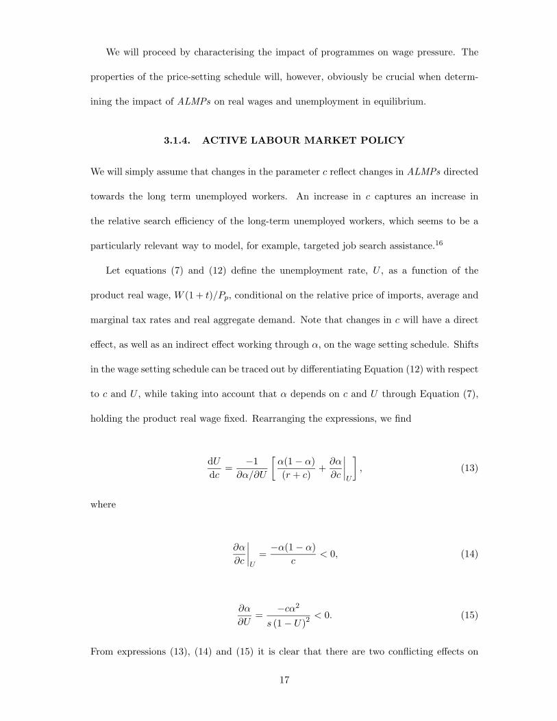
Let equations (7) and (12) define the unemployment rate, U , as a function of the

product real wage, W (1 + t)/Pp, conditional on the relative price of imports, average and

marginal tax rates and real aggregate demand. Note that changes in c will have a direct

effect, as well as an indirect effect working through α, on the wage setting schedule. Shifts

in the wage setting schedule can be traced out by differentiating Equation (12) with respect

to c and U , while taking into account that α depends on c and U through Equation (7),

holding the product real wage fixed. Rearranging the expressions, we find

dU

dc=

−1

∂α/∂U

[

α(1 − α)

(r + c)+

∂α

∂c

∣

∣

∣

∣

U

]

, (13)

where

∂α

∂c

∣

∣

∣

∣

U

=−α(1 − α)

c< 0, (14)

∂α

∂U=

−cα2

s (1 − U)2< 0. (15)

From expressions (13), (14) and (15) it is clear that there are two conflicting effects on

17

the wage setting schedule following a higher c. The first term in the square brackets of

Equation (13) tends to increase the wage pressure. Higher wage demands follows because a

higher c increases the welfare associated with long term unemployment. The second term

captures the impact of c channelled through α. A higher c implies that the long-term

unemployed compete more efficiently with the short-term unemployed for the available

jobs. This reduces the value of short-term unemployment; lower wage demands follow as

a consequence.17

One can, however, note that the size of the discount rate is crucial in determining

which of the two effects that will dominate in this simplified framework. When the future

is discounted, i.e., r > 0, the impact on welfare associated with short-term unemployment

will dominate over the impact on welfare associated with long term unemployment. Thus,

wage demands will be reduced due to the higher competition over jobs facing an employed

worker in case of unemployment. In this model, ALMPs that increase the search efficiency

of all unemployed workers, will have no influence on wage pressure and unemployment.

4. EMPIRICAL MODELLING STRATEGIES

The main focus in this paper is on wage setting. Thus, our primary interest lies in finding

a structural relationship between the factors influencing the behaviour of wage setting

agents and the outcome, in our case a bargaining outcome, in terms of a desired real wage

rate. The issue is how to model such a structural equation. This issue, in turn, involves a

lot of decisions. Below, we will outline a number of such issues and motivate the decisions

we have made.

18

4.1. STATIC VERSUS DYNAMIC MODELLING

The theoretical framework outlined above is static, in the sense that we focus on the steady

state equilibrium of the model. Hence, our theoretical predictions pertain to steady-state

effects. There are, however, a number of good reasons to believe that what we observe in

our data may involve a mix of equilibria and adjustments to such equilibria.18 Lacking

explicit predictions about the dynamic paths of variables, we mainly use our theoretical

model to suggest (testable) restrictions defining equilibria, whereas we let the dynamics

be suggested by the data.

An alternative would be to impose rather than to test the equilibrium model, and use

some estimator that is consistent in the presence of non-Gaussian error terms. A drawback

with this approach in our case is that preliminary tests indicate that most of the variables

of interest may be non-stationary. Valid inference requires stationarity, which in our case

would imply estimating on differenced data. This, in turn, destroys valuable long-run

information in the data.

A second alternative would, of course, be to derive dynamics from theory. We are,

however, inclined to believe that whereas good theory may be informative about long-run

equilibrium relationships among variables, this is not so to the same extent when it comes

to dynamics.

Our modelling strategy is, therefore, to extract long-run equilibrium information from

the data by looking for theory-consistent cointegrating vectors, and in addition to extract

short-run information on dynamic adjustments by estimating error-correction models.

4.2. SYSTEMS VERSUS SINGLE-EQUATIONS METHODS

The first generation of studies employing error-correction techniques relied on single-

equation methods. Recently, systems methods have become increasingly popular, in part

19

because of advances in econometric theory19, in part because systems methods have be-

come available in standard time-series econometrics packages.20 Both approaches have

their pros and cons.

The main drawback of systems modelling is that the short samples available in most

applications (including ours) put a severe constraint on the number of variables that can

be modelled. We could without problems, using our theoretical framework and previous

empirical studies of wage setting, motivate the inclusion of more than 10 variables in the

analysis. Given 38 annual observations, such an analysis is simply not feasible. Thus, only

a subset of the a priori interesting variables can be modelled consistently as a system.

We describe below how we chose our subset. The systems approach, however, also has

important advantages.

First, it provides a consistent framework for finding the number of long-run relations

(cointegrating vectors) among a set of variables. Moreover, since the cointegrating vec-

tors are not uniquely determined by data alone, the analyst is forced to make explicit

assumptions to identify them. These assumptions imply restrictions, which are testable.

Second, a major problem with the single-equations approach is that one has to rely on

assumptions about exogeneity that are either not tested (in the case of OLS estimation) or

hard to test (instrumental variables, IV, estimation).21 In the framework of a system, on

the other hand, exogeneity tests are an integral part of the estimation procedure. Actually,

one possible outcome of the systems approach is that it may be shown that OLS can be

applied to the equation of interest without loss of information. The results of the systems

modelling, employing Johansen’s (1988) FIML methods are presented in Section 6.1.

Because of the constraints with respect to the number of variables that can be in-

cluded in the systems modelling, we also estimate (by IV methods) single-equation error-

correction models of wage setting. In addition to permitting a larger number of potentially

20

important variables, this approach also allows us to estimate the model recursively. This,

in turn, provides important information on parameter (in)stability. This sheds light on

the questions raised in the introduction relating to possible changes in i.a. the sensitivity

of wage setters to labour market conditions such as unemployment and ALMPs. The

estimated error-correction models are presented in Section 7.3.

Both systems methods and single-equation error-correction models rely on correctly

specified dynamics for reliable inference about long-run relationships.22 Park (1992) sug-

gests a way to estimate cointegrating relationships, canonical cointegrating regressions,

that employs non-parametric methods to transform the data in a way that allows valid

inference based on OLS regressions on the transformed data. The method and the results

derived by it are presented in Section 7.4.

5. THE DATA

Our data set consists of annual data over the period 1960–1997. We use annual data partly

to cover as long a time span as possible in order to be able to analyse long-run properties

of the variables, partly because there is no variation during a year in some of our variables

(for example the income tax rates) and partly to avoid the measurement errors present in

higher-frequency series. In this section, we provide data definitions and sources and some

descriptive statistics related to the properties of the series used in the empirical study.23

5.1. WAGES

The nominal hourly wage measure used pertains to the business sector and is generated as

the ratio between the total wage sum (including employers’ contributions to social security,

henceforth called payroll taxes) and the total number of hours worked by employees in the

business sector. To get the product real wage, the wage series is deflated by a measure

21

of producer prices. The price series used is the implicit deflator for value added in the

business sector at producer prices. The log of the product real wage is denoted by w− pp.

Finally, to get the measure of labour’s share of value added, which is what we end up using

in most of the empirical work, we divide the product real wage rate by average labour

productivity.24 The latter variable is derived by dividing real value added in the business

sector by the total number of hours worked (including the hours worked by employers and

self-employed). The data are taken from the National Accounts Statistics.25 The use of

the National Accounts Statistics is dictated by our wish to cover the whole business sector,

for which no direct measure of the hourly wage rate is available for our period.


The (natural) logarithm of labour’s share of value added, (w − q),26 is plotted in

Figure 3. The series is upward trended from the early 1960s to the early 1980s. Following

the two devaluations in 1981 and 1982 as well as in the aftermath of the depreciation of the

Krona in the early 1990s, the share falls very rapidly. Unit-root tests reported in Table 2

suggest that the labour share of value added may be an I (1) variable.27


5.2. UNEMPLOYMENT

The number of unemployed persons is the standard measure given by the Labour Force

Surveys (LFS ) performed by Statistics Sweden.28 This number of persons is turned into

an unemployment rate by relating it to the labour force. The measure of the labour force

is not the one supplied by the LFS. Instead, the labour force is derived as the sum of

employment according to the National Accounts Statistics, unemployment according to

the LFS and participation in active labour market policy measures (ALMPs) according

22

to statistics from the National Labour Market Board.29 This “non-standard” definition of

the labour force is used first because the LFS measure is not available prior to 1963 and

second because it seems natural to include programme participants in the measure of the

labour force, as active job search and joblessness are necessary conditions for programme

eligibility.

The log of the unemployment rate, u, is graphed in Figure 430. The variation in the

unemployment rate is completely dominated by the dramatic rise in the early 1990s. Prior

to this the series exhibits a clear cyclical pattern with every peak slightly higher than its

predecessor. Looking at Table 2, we see that unit roots cannot be rejected, even allowing

for a deterministic trend, whereas they are rejected for the series in first-difference form.

This would indicate that the (logged) unemployment rate behaves like an I (1) series in

our sample period. It is, however, important to remember that the failure to reject the

null of non-stationarity does not entail accepting a unit root; it may, for example, reflect

other forms of non-modelled non-stationarity such as regime shifts.


5.3. LABOUR MARKET PROGRAMMES

The programmes include the major ones administered by the National Labour Market

Board. Until 1984 these are labour market training and relief work. In 1984 youth pro-

grammes and recruitment subsidies are added. During the 1990s a vast number of new

programmes were introduced. Of these, we have included training replacement schemes,

workplace introduction (API) and work experience schemes (ALU). The source of all data

on ALMPs is the National Labour Market Board. The variable used to represent ALMPs

is the accommodation ratio, which relates the number of programme participants to the

sum of open unemployment and ALMP participation. The log of the accommodation rate,

23

γ, is displayed in Figure 5. The series shows a steep upward trend until the late 1970s,

then varies cyclically over the 1980s and falls sharply from the late 1980s, despite the fact

that the number of participants reached an all times high during this period. Unit root

tests reported in Table 2 fail to reject a unit root in the (logged) levels, whereas unit roots

are forcefully rejected in the logarithmic difference series, leading us to treat the variable

as potentially I (1).


5.4. TAXES

The taxes in our data set are income taxes, payroll taxes and indirect taxes, i.e., the

tax components of the tax-price wedge between product and consumption real wages.

There are many possible ways to compute taxes. Details on on how our tax measures are

derived are given in an appendix available on request. The income tax rate is computed

for the tax brackets corresponding to the average annual labour income in the business

sector according to the National Accounts Statistics to achieve consistency with the wage

measures used. The payroll tax factor31 is computed as the ratio between the total wage

bill in the business sector according to the National Accounts Statistics, including and

excluding employers’ contributions. Finally, the indirect tax factor32 is computed as the

ratio between value added in the business sector at market prices and at producer prices

according to the National Accounts Statistics.

The log of the tax wedge, defined as θ ≡ log(1+ t)+ log(1+V AT )− log(1−at), where

t is the payroll tax rate, V AT the indirect tax rate and at the average income tax rate, is

plotted in Figure 6. The wedge increases almost monotonically until the tax reform of the

early 1990s, when it falls considerably and then stays fairly constant. Unit root tests in

Table 2 (with and without trend included) do not reject the null of a unit root in levels,

24

whereas the first difference seems to be stationary. Also in this case, thus, the series will

be treated as potentially I (1).


We have also computed a point estimate of marginal income tax rates pertaining to

the tax bracket at which the average tax rate is computed. This marginal tax rate is used

to derive our measure of progressivity in the income tax system, the coefficient of residual

income progressivity, RIP .

The logged series is plotted in Figure 7. Progressivity remained fairly unchanged from

the beginning of our sample period until the early 1970s, when it increased rapidly for a

number of years. This increase was halted in 1978, when a steady decrease in progressivity

culminated in the 1991 tax reform, when most progressivity was removed. Since then, little

has happened. The series is serially correlated, but almost all serial correlation is removed

by first-differencing. The ADF tests in Table 2 do not reject a unit root in the series.


5.5. THE RELATIVE PRICE OF IMPORTS

In addition to taxes, the wedge between the product real wage and the consumption real

wage reflects the relative price of imports. We measure this variable by the implicit deflator

of imports relative to the implicit deflator of value added at producer prices according to

the National Accounts Statistics.

The (log) relative price of imports, pI − pp, plotted in Figure 8, first falls until 1972.

The first oil price shock pushes the relative price steeply upwards, and subsequently, the

devaluations of the late 1970s and early 1980s coincide with a continuous rise. This is

reversed after the devaluation in 1982, after which domestic prises rise faster than import

25

prices for 10 years. Finally, the depreciation of the Krona in 1990s accompanies a reversal

of this trend. The unit root tests in Table 2, which reject for the differenced series but

not for the series in logs, suggest that it may be appropriate to treat the relative price of

imports as first-order integrated.


5.6. THE REPLACEMENT RATE IN THE UNEMPLOYMENT

INSURANCE SYSTEM

The final variable modelled in our system is the replacement rate in the unemployment in-

surance system. We measure it by the maximum daily before-tax compensation, converted

into an annual compensation, in relation to the average annual before-tax labour income in

the business sector33. Without going into too much details, we just want to point out that

this implicitly assumes that the representative union member is entitled to the maximum

level of compensation, which according to rough calculations seems reasonable.34

The log of the replacement rate, ρ, is reproduced in Figure 9. The replacement rate,

according to our measure, shows a trend wise increase until the early 1990s, after which

point it decreases rather rapidly. It can also be noted that the variations around the trend

are quite large. Once more, unit root tests reported in Table 2 indicate that the series

may be I (1).


6. SYSTEMS MODELLING

Our general approach to the empirical modelling is to start out from an unrestricted vector-

autoregressive (V AR) representation of the variables we study. Two critical choices have

26

to be made. First, which variables should be included, and second, which lag length should

be chosen.35 In the first of these respects, we have mainly been guided by our theoretical

framework, but also, to some extent, by previous empirical studies of Swedish aggregate

wage setting. The determination of the lag length is discussed below.

The model presented in Section 3.1 gave rise to two equilibrium relationships between

the real wage rate and unemployment: the wage-setting (WS ) schedule and the price-

setting (PS ) schedule.

The discussion of the properties of the price-setting schedule in Section 3.1.3 suggested

that price setters potentially would respond to the unemployment rate and the relative

price of imports, but that the signs of the responses would be indeterminate:

w − pp = f(?u,

?

(pI − pp)), (16)

where lower-case letters denote (natural) logarithms of the corresponding upper-case letters

and the question marks denote the uncertainty of the sign of the effect. One further result

from the theoretical analysis was that the price-setting schedule is unaffected by changes

in average labour productivity and the tax wedge between product and consumption real

wages. Also notice that Equation (16), as long as the effect of the relative import price is

non-zero, can be renormalised as

pI − pp = F (u, w − pp) (17)

The corresponding results for the wage-setting schedule are summarised in the following

equation:

w − pp = g(−

u,+(?)

(pI − pp),+ρ,

+q,

+RIP ,

+θ,

?γ). (18)

27

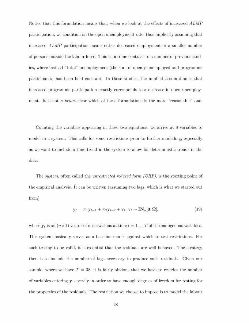
Notice that this formulation means that, when we look at the effects of increased ALMP

participation, we condition on the open unemployment rate, thus implicitly assuming that

increased ALMP participation means either decreased employment or a smaller number

of persons outside the labour force. This is in some contrast to a number of previous stud-

ies, where instead “total” unemployment (the sum of openly unemployed and programme

participants) has been held constant. In those studies, the implicit assumption is that

increased programme participation exactly corresponds to a decrease in open unemploy-

ment. It is not a priori clear which of these formulations is the more “reasonable” one.

Counting the variables appearing in these two equations, we arrive at 8 variables to

model in a system. This calls for some restrictions prior to further modelling, especially

as we want to include a time trend in the system to allow for deterministic trends in the

data.

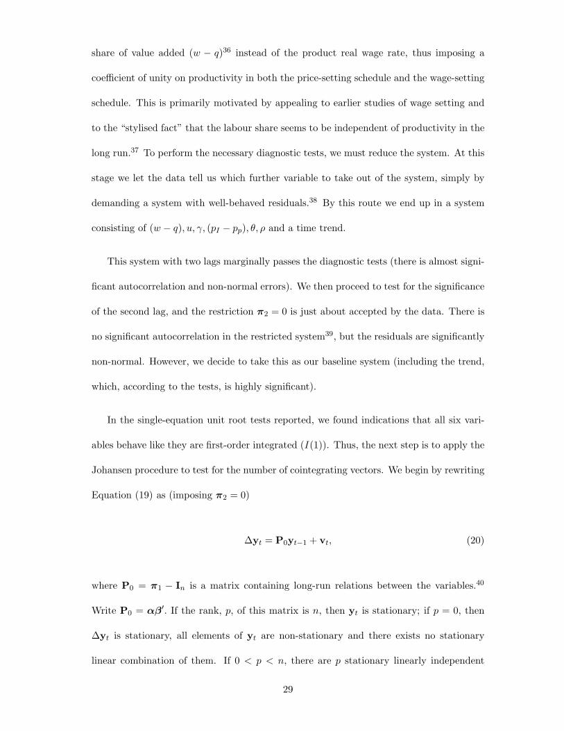
The system, often called the unrestricted reduced form (URF), is the starting point of

the empirical analysis. It can be written (assuming two lags, which is what we started out

from)

yt = π1yt−1 + π2yt−2 + vt, vt v INn[0,Ω], (19)

where yt is an (n×1) vector of observations at time t = 1 . . . T of the endogenous variables.

This system basically serves as a baseline model against which to test restrictions. For

such testing to be valid, it is essential that the residuals are well behaved. The strategy

then is to include the number of lags necessary to produce such residuals. Given our

sample, where we have T = 38, it is fairly obvious that we have to restrict the number

of variables entering y severely in order to have enough degrees of freedom for testing for

the properties of the residuals. The restriction we choose to impose is to model the labour

28

share of value added (w − q)36 instead of the product real wage rate, thus imposing a

coefficient of unity on productivity in both the price-setting schedule and the wage-setting

schedule. This is primarily motivated by appealing to earlier studies of wage setting and

to the “stylised fact” that the labour share seems to be independent of productivity in the

long run.37 To perform the necessary diagnostic tests, we must reduce the system. At this

stage we let the data tell us which further variable to take out of the system, simply by

demanding a system with well-behaved residuals.38 By this route we end up in a system

consisting of (w − q), u, γ, (pI − pp), θ, ρ and a time trend.

This system with two lags marginally passes the diagnostic tests (there is almost signi-

ficant autocorrelation and non-normal errors). We then proceed to test for the significance

of the second lag, and the restriction π2 = 0 is just about accepted by the data. There is

no significant autocorrelation in the restricted system39, but the residuals are significantly

non-normal. However, we decide to take this as our baseline system (including the trend,

which, according to the tests, is highly significant).

In the single-equation unit root tests reported, we found indications that all six vari-

ables behave like they are first-order integrated (I (1)). Thus, the next step is to apply the

Johansen procedure to test for the number of cointegrating vectors. We begin by rewriting

Equation (19) as (imposing π2 = 0)

∆yt = P0yt−1 + vt, (20)

where P0 = π1 − In is a matrix containing long-run relations between the variables.40

Write P0 = αβ′. If the rank, p, of this matrix is n, then yt is stationary; if p = 0, then

∆yt is stationary, all elements of yt are non-stationary and there exists no stationary

linear combination of them. If 0 < p < n, there are p stationary linearly independent

29

linear combinations of yt, and both α(n×p) and β′

(p×n) have rank p. Thus, the problem of

finding the number of cointegrating vectors consists of finding the rank of P0.

It is fairly obvious that the wage-setting schedule is not identified without further

parameter restrictions.41 It may still, however, be the case that the model is identified

in an empirical sense: the data may accept further restrictions on parameters that actu-

ally identifies the model. What we would need is something that shifts the price-setting

schedule without affecting the wage-setting schedule. We report the results of our efforts

in that direction in Section 6.1 below.

6.1. EMPIRICAL RESULTS

The Johansen procedure indicates that there may be 2 or 3 cointegrating vectors, i.e.

rank(P0) is 2 or 3, see Table 3. Although most tests indicate that the number is 2,

and although our theoretical discussion identified 2 potential cointegrating relations, we

choose 3 cointegrating vectors as our baseline case. The main reason is that we do not get

any reasonable results by pursuing the analysis under the assumption of 2 cointegrating

vectors, see Section 6.1.5 below.

As we hinted at above, even though the number of cointegrating vectors is unique,

the vectors themselves are not without further restrictions. To see this, note that αβ′ =

αγ−1γβ′ = α∗β∗′

for any non-singular (p × p) matrix γ.


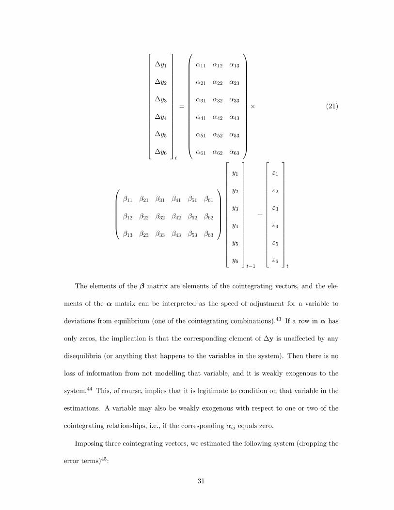
Our preferred model assumes that we have 3 cointegrating vectors. In this case, the

dimension of α is (6 × 3) and that of β′

is (3 × 6). Hence, the system may be written42

30

∆y1

∆y2

∆y3

∆y4

∆y5

∆y6

t

=

α11 α12 α13

α21 α22 α23

α31 α32 α33

α41 α42 α43

α51 α52 α53

α61 α62 α63

× (21)

β11 β21 β31 β41 β51 β61

β12 β22 β32 β42 β52 β62

β13 β23 β33 β43 β53 β63

y1

y2

y3

y4

y5

y6

t−1

+

ε1

ε2

ε3

ε4

ε5

ε6

t

The elements of the β matrix are elements of the cointegrating vectors, and the ele-

ments of the α matrix can be interpreted as the speed of adjustment for a variable to

deviations from equilibrium (one of the cointegrating combinations).43 If a row in α has

only zeros, the implication is that the corresponding element of ∆y is unaffected by any

disequilibria (or anything that happens to the variables in the system). Then there is no

loss of information from not modelling that variable, and it is weakly exogenous to the

system.44 This, of course, implies that it is legitimate to condition on that variable in the

estimations. A variable may also be weakly exogenous with respect to one or two of the

cointegrating relationships, i.e., if the corresponding αij equals zero.

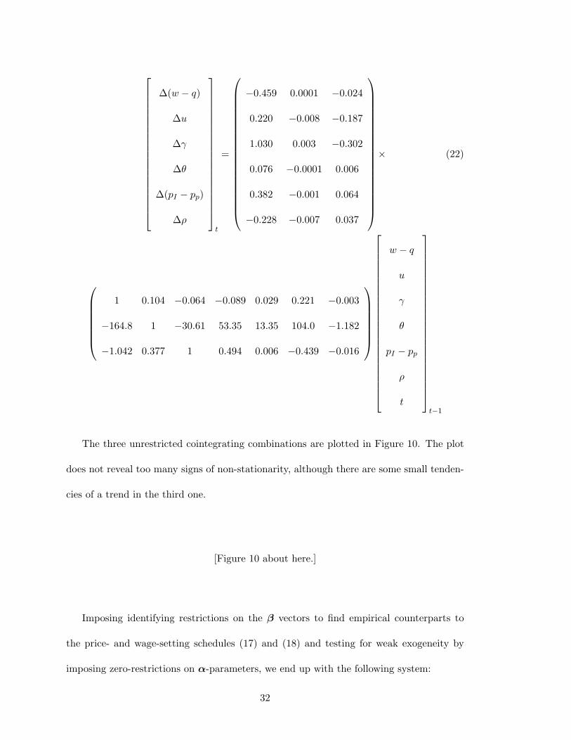
Imposing three cointegrating vectors, we estimated the following system (dropping the

error terms)45:

31

∆(w − q)

∆u

∆γ

∆θ

∆(pI − pp)

∆ρ

t

=

−0.459 0.0001 −0.024

0.220 −0.008 −0.187

1.030 0.003 −0.302

0.076 −0.0001 0.006

0.382 −0.001 0.064

−0.228 −0.007 0.037

× (22)

1 0.104 −0.064 −0.089 0.029 0.221 −0.003

−164.8 1 −30.61 53.35 13.35 104.0 −1.182

−1.042 0.377 1 0.494 0.006 −0.439 −0.016

w − q

u

γ

θ

pI − pp

ρ

t

t−1

The three unrestricted cointegrating combinations are plotted in Figure 10. The plot

does not reveal too many signs of non-stationarity, although there are some small tenden-

cies of a trend in the third one.


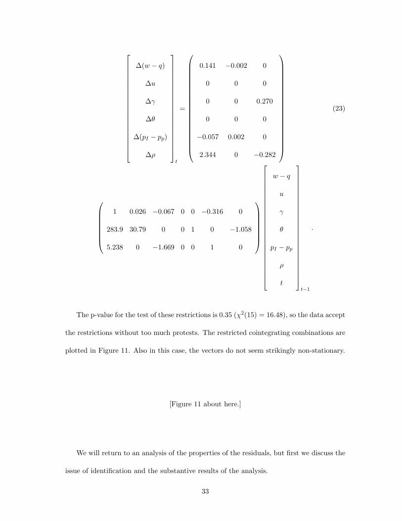
Imposing identifying restrictions on the β vectors to find empirical counterparts to

the price- and wage-setting schedules (17) and (18) and testing for weak exogeneity by

imposing zero-restrictions on α-parameters, we end up with the following system:

32

∆(w − q)

∆u

∆γ

∆θ

∆(pI − pp)

∆ρ

t

=

0.141 −0.002 0

0 0 0

0 0 0.270

0 0 0

−0.057 0.002 0

2.344 0 −0.282

(23)

1 0.026 −0.067 0 0 −0.316 0

283.9 30.79 0 0 1 0 −1.058

5.238 0 −1.669 0 0 1 0

w − q

u

γ

θ

pI − pp

ρ

t

t−1

.

The p-value for the test of these restrictions is 0.35 (χ2(15) = 16.48), so the data accept

the restrictions without too much protests. The restricted cointegrating combinations are

plotted in Figure 11. Also in this case, the vectors do not seem strikingly non-stationary.


We will return to an analysis of the properties of the residuals, but first we discuss the

issue of identification and the substantive results of the analysis.

33

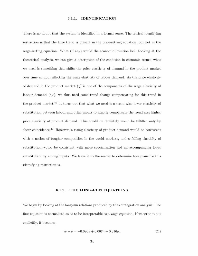
6.1.1. IDENTIFICATION

There is no doubt that the system is identified in a formal sense. The critical identifying

restriction is that the time trend is present in the price-setting equation, but not in the

wage-setting equation. What (if any) would the economic intuition be? Looking at the

theoretical analysis, we can give a description of the condition in economic terms: what

we need is something that shifts the price elasticity of demand in the product market

over time without affecting the wage elasticity of labour demand. As the price elasticity

of demand in the product market (η) is one of the components of the wage elasticity of

labour demand (εN ), we thus need some trend change compensating for this trend in

the product market.46 It turns out that what we need is a trend wise lower elasticity of

substitution between labour and other inputs to exactly compensate the trend wise higher

price elasticity of product demand. This condition definitely would be fulfilled only by

sheer coincidence.47 However, a rising elasticity of product demand would be consistent

with a notion of tougher competition in the world markets, and a falling elasticity of

substitution would be consistent with more specialisation and an accompanying lower

substitutability among inputs. We leave it to the reader to determine how plausible this

identifying restriction is.

6.1.2. THE LONG-RUN EQUATIONS

We begin by looking at the long-run relations produced by the cointegration analysis. The

first equation is normalised so as to be interpretable as a wage equation. If we write it out

explicitly, it becomes

w − q = −0.026u + 0.067γ + 0.316ρ. (24)

34

Thus, in the long run there is a negative relationship between labour’s share of value

added and the unemployment rate, a positive relationship between the share and the

accommodation ratio and a positive relation between the share and the replacement rate

in the unemployment insurance system. The point estimate of the long-run effect of

unemployment on wage setting is rather low compared to most previous estimates (see

Section 2), which might indicate that the prolonged period of high unemployment rates

in the 1990s has affected wage setting institutions adversely. The estimated positive effect

of ALMPs is, on the other hand, rather similar to what has been found in earlier studies.

The implication is that the wage-push mechanism identified in Section 3.1.4 seems to

dominate the “job-competition” effect.48 Effects of the unemployment insurance system

have been notoriously difficult to detect in studies using aggregate data. Here we find a

rather strong positive relationship between wages and the replacement rate. Finally, it is

worth noting that one effect is ‘conspicuous by its absence’: we test and do not reject the

restriction of no long-run wage effects49 of the wedge between the product real wage and

the consumption real wage.

The second cointegrating vector has been normalised to be interpreted as a price-setting

equation, where the price is the relative price between imports and production.50 We get

the following long-run equation:

pI − pp = −283.9(w − q) − 30.79u + 1.058t. (25)

Interpreting a higher wage share, (w− q), as a “cost push”, such a cost push increases the

price of domestic goods in the long run.51 A rise in unemployment, a negative “demand

shock”52, increases the relative price of domestic goods. According to the price-setting

rule in Section 3.1.3, this implies increasing returns to scale. Finally, the relative price

35

of imports follows a rising trend. We have no good theory-based explanation to this, al-

though, as we noted in Section 6.1.1, this is consistent with Swedish firms facing increasing

competition in the world market. We still feel (at least somewhat) confident about the

interpretation of this equation, since the data do not reject the restrictions that potential

effects of taxes, unemployment insurance and labour market programmes go through their

effects on wages.

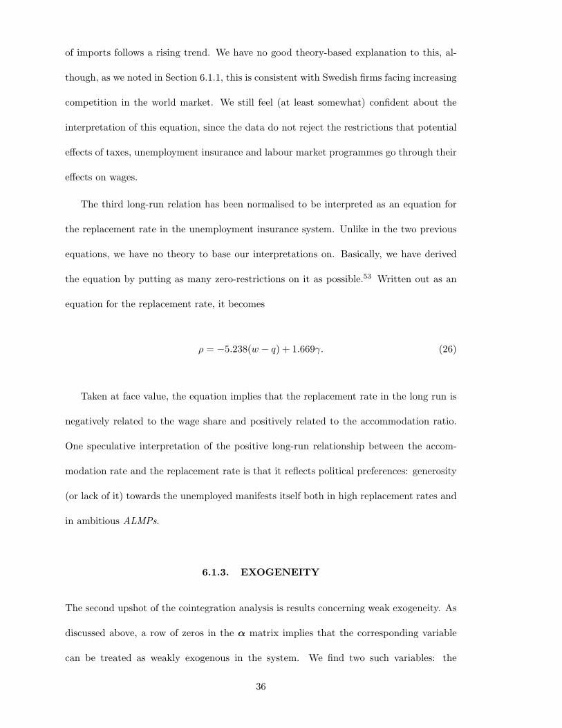
The third long-run relation has been normalised to be interpreted as an equation for

the replacement rate in the unemployment insurance system. Unlike in the two previous

equations, we have no theory to base our interpretations on. Basically, we have derived

the equation by putting as many zero-restrictions on it as possible.53 Written out as an

equation for the replacement rate, it becomes

ρ = −5.238(w − q) + 1.669γ. (26)

Taken at face value, the equation implies that the replacement rate in the long run is

negatively related to the wage share and positively related to the accommodation ratio.

One speculative interpretation of the positive long-run relationship between the accom-

modation rate and the replacement rate is that it reflects political preferences: generosity

(or lack of it) towards the unemployed manifests itself both in high replacement rates and

in ambitious ALMPs.

6.1.3. EXOGENEITY

The second upshot of the cointegration analysis is results concerning weak exogeneity. As

discussed above, a row of zeros in the α matrix implies that the corresponding variable

can be treated as weakly exogenous in the system. We find two such variables: the

36

unemployment rate and the tax wedge. The latter can be understood as a statement that

tax rates are determined in the political system in a way that is not systematically related

to the variables in our system.

It may at first sight seem surprising that the unemployment rate turns out to be weakly

exogenous. Our interpretation of the result is that it may reflect the fact that we have not

specified a full equilibrium model: we have neither imposed any external balance condition

nor included any measure of balance of payments in the empirical analysis. The extension

of the information set induced by adding new variables could turn the exogeneity result

around. This means that, e.g., macroeconomic policies may influence the unemployment

rate in ways that are given from the perspective of the model we have set up but not

relative to a more general model.

The exogeneity result is to some extent “good news”, in the sense that, relative to

the variables we analyse, we can condition on the unemployment rate, which in turn is

related to the possibility to identify a wage-setting equation in the single-equation models

we estimate later. On the other hand, it is not so good news from the perspective of the

theoretical model presented Section 3.

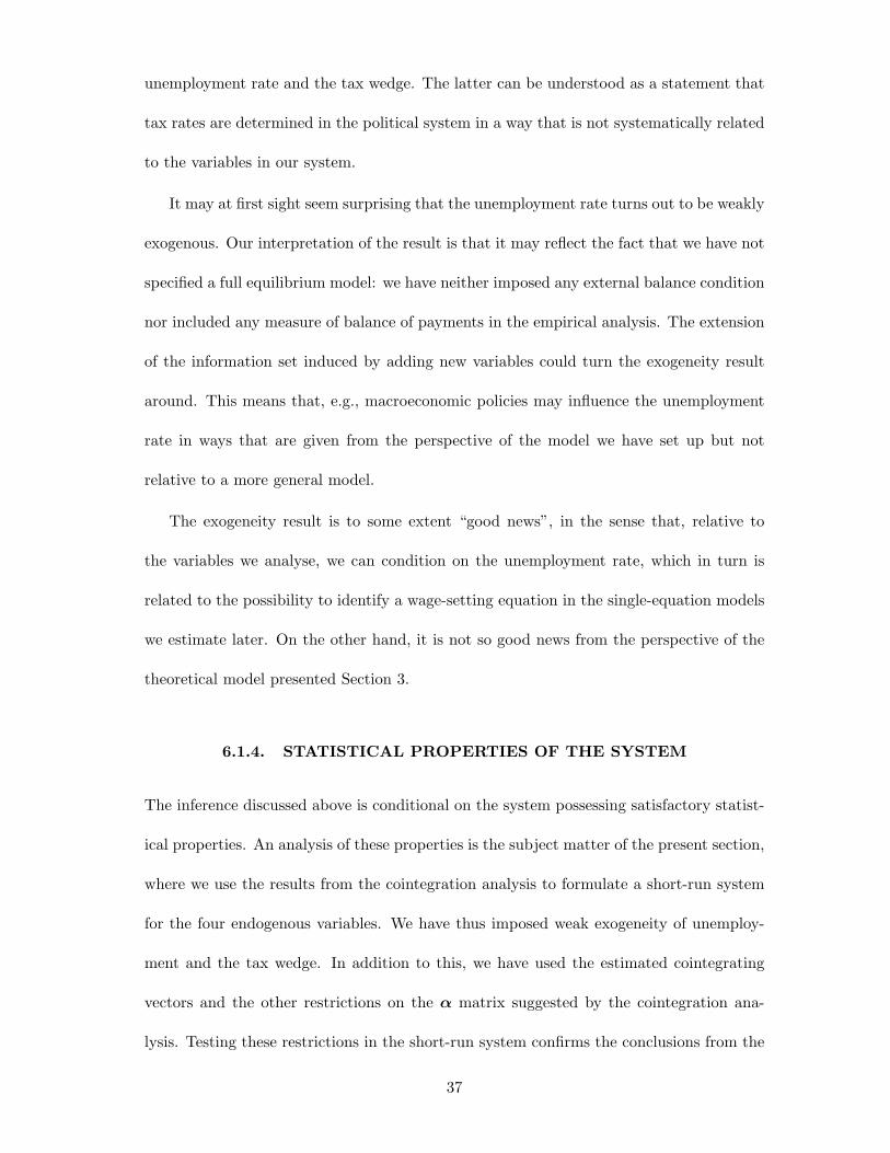
6.1.4. STATISTICAL PROPERTIES OF THE SYSTEM

The inference discussed above is conditional on the system possessing satisfactory statist-

ical properties. An analysis of these properties is the subject matter of the present section,

where we use the results from the cointegration analysis to formulate a short-run system

for the four endogenous variables. We have thus imposed weak exogeneity of unemploy-

ment and the tax wedge. In addition to this, we have used the estimated cointegrating

vectors and the other restrictions on the α matrix suggested by the cointegration ana-

lysis. Testing these restrictions in the short-run system confirms the conclusions from the

37

cointegration analysis: the restrictions on the short-run system implied by the previous

analysis are not rejected. Thus, we feel confident about conditioning on unemployment

and the tax wedge.

We have, however, not attempted to model the short-run dynamics of the whole system

by looking for contemporary effects of the endogenous variables. Thus, apart from the long-

run relations, which we want to interpret as structural equations corresponding (in the

case of the price- and wage-setting equations) to equations in our theoretical modelling,

we do not want to give any structural interpretation of our short-run equations. We

mainly estimate them to show that the resulting system possesses satisfactory statistical

properties.

The statistical properties, as measured by tests for residual autocorrelation, normality

and heteroscedasticity reveal problems with normality for the system as a whole, and

looking at single equations, the problems arise in the equation for the relative price. System

tests do not indicate problems with either autocorrelation or heteroscedasticity, although

there is significant heteroscedasticity in the equation for the replacement rate. More

information on the estimated system and some of the diagnostic tests are reproduced in

an appendix available on request. The actual and fitted values and scaled residuals are

reproduced in Figure 12.


6.1.5. SENSITIVITY ANALYSIS

How robust are the results presented above? We have performed some “sensitivity ana-

lysis”, where we try a number of alternative sets of identifying restrictions. A first set of

tests pertain to the third cointegrating relation, where we look for a cointegrating rela-

tion with some natural interpretation. More specifically, we look for a third cointegrating

38

relation that can be interpreted as a “budget constraint”. Thus, we look for a possible

negative relationship between the generosity of the unemployment insurance system and

the volume of ALMPs, and we want this trade-off to be shifted downwards (upwards) by

a decreasing (increasing) tax base. We also analyse the possible different wage- and price-

setting relations that pass tests, given the third cointegrating relation presented in the

baseline case above. Our second set of tests assumes that we instead of three cointegrat-

ing vectors have two. Under this assumption we examine whether our estimated long-run

wage-setting relation changes substantially or is mainly unchanged. In both sets of tests,

we restrict the analysis to restrictions that pass tests and where the first two relations

have clear interpretations as wage- and price-setting relations.

THREE COINTEGRATING VECTORS The set-up in the analysis where we as-

sume that there are three cointegrating vectors is that we impose the same restrictions on

the α-matrix as in the baseline case above. Furthermore, we let the third cointegrating

vector be rather “freely” estimated—we only restrict the analysis to relations where the

relative price is excluded. Briefly, the results are negative with respect to the third coin-

tegrating relation. We never end up with cointegrating vectors that can be interpreted as

budget constraints, and the resulting “cointegrating” combinations generally look “more”

non-stationary than the unrestricted combination plotted in Figure 10. Fixing the third

cointegrating relation and concentrating on wage- and price-setting relations, we find four

different sets of restrictions that pass tests (including the baseline case above). In these

cases, the coefficient on programme participation either is in the same magnitude as in

the baseline case above or zero. Thus, we find a weak wage-pushing effect of programmes,

but we cannot rule out that there is no effect at all.

39

TWO COINTEGRATING VECTORS Looking at systems under the assumption

of two cointegrating vectors leaves us with three possible systems that pass all tests. They

are fairly similar, and are all characterised by what we find unreasonable point estimates.

In particular, we find an extremely strong upward push on wages from the replacement

rate in the UI system, and a similarly extremely strong wage moderation from ALMPs.54

We find these effects too extreme to be taken seriously, and stick to the case with three

cointegrating vectors as our preferred one.

6.2. CONCLUDING COMMENTS ON THE ESTIMATED SYSTEMS

Our main finding related to wage setting and ALMPs is that there may be a small wage-

raising effect of ALMPs, but we cannot strongly rule out that the effect equals zero.

Furthermore, we have found a long-run effect of unemployment on wages that is somewhat

lower than most previous estimates. The result that the tax wedge does not matter for wage

pressure in the long run is somewhat at odds with most previous studies, as is the estimated

fairly strong long-run positive covariation between real wages and the replacement rate in

the UI system.

We have also found that both the unemployment rate and the tax wedge between the

product real wage and the consumption real wage are weakly exogenous with respect to

the variables that we have analysed. The former finding, which seems fairly robust, implies

that we can in fact identify a structural wage-setting relation in the data.55

On the other hand, some of the estimated effects are non-robust to changes in specific-

ations, and we end up with a preferred system where we can only give some theory-based

interpretation of two of the three identified cointegrating vectors.

40

7. SINGLE EQUATIONS MODELLING

7.1. INTRODUCTION

The main drawback with systems modelling, as discussed above, is that the limited number

of observations severely constrains the number of variables that can enter the analysis. Our

strategy in this section is to look closer at the wage-setting relation in a single-equation

context, making use of the results from the systems analysis. The analysis in this section

will naturally also draw on the theoretical analysis, where some variables that were not

modelled in the systems context were discussed. Finally, we will also relate our analysis

to earlier attempts to model aggregate Swedish wage setting with a focus on the role of

ALMPs.

Starting with the theoretical analysis, the upshot of Equation (12) in log-linearised

form is a wage-setting relation of the following form (letting lower-case letters represent

natural logarithms):

w − pp = a0 + a1q − a2u + a3γ + a4θ + a5(pI − pp) + a6rip + a7ρ, (27)

where w − pp is the product real wage rate, q productivity, u the unemployment rate, γ

the accommodation ratio, θ the tax wedge, (pI − pp) the relative price of imports, rip the

measure of residual income progressivity and ρ the replacement rate in the unemployment

insurance system. We expect all parameters except a1 and a3 (which can be either positive

or negative) to be non-negative.

Our primary interest in Equation (27) is in looking at the effect of ALMPs on wage

setting. Thus, we will especially focus on the estimate of a3. We will both compare this

estimate to effects found in earlier studies and look at the evolution of the parameter over

41

time to determine whether our finding in the systems analysis of a rather small effect

reflects changing labour market conditions and/or the new policy mix in the 1990s or if it

primarily is driven by differences in model specification or by new data series.

A number of special cases of Equation (27) can be found, either from theory by im-

posing restrictions on technology or union objectives, or by looking at “stylised facts” or

empirical findings in earlier studies. In addition, a number of policy questions are related

to some of these restrictions. Some of these issues will be brought up in the presentation

of the results.

7.2. EMPIRICAL SPECIFICATION OF DYNAMIC BASELINE

MODEL

Following the analysis in previous sections, we treat the variables in Equation (27) as

potentially first-order integrated. Thus, we must formulate the econometric model in

such a way that non-stationary variables are transformed into stationary ones. This can

be achieved either by taking first-differences of potentially I (1) variables or by forming

stationary (i.e. cointegrating) combinations of them. Taking first differences destroys

valuable long-run information. Hence, our strategy is to find stationary linear combinations

of the variables.

This can, in turn, either be achieved by the two-step Engle & Granger (1987) procedure

or by a one-step procedure, where the lagged potentially cointegrated variables are entered

as single explanatory variables in a regression with the dependent variable in first-difference

form.

As there is some evidence that the small-sample properties of the one-step approach

are better (Banerjee et al. 1993), we follow this approach.56 The baseline transformation

42

we use is the following57:

∆(w − pp)t = b0 + b1(w − pp)t−1 + b2qt−1 + b3ut−1 + b4γt−1 (28)

+b5θt−1 + b6(pI − pp)t−1 − b7ript−1 + b8ρt−1 +

b9∆qt + b10∆ut + b11∆γt + b12∆θt + b13∆(pI − pp)t

−b14∆ript + b15∆ρt + b16∆(w − pp)t−1 + εt.

This model was estimated by OLS and IV methods, and in both cases passed diagnostic

tests.58 Plots of recursive parameter estimates did not indicate any substantial problems

of parameter instability. Given these results, we take the estimates of Equation (28) as

our benchmark for further testing.

7.3. RESULTS

We start by testing whether the product real wage is unit elastic with respect to pro-

ductivity in the long run. This is equivalent to testing the restriction b1 = −b2.59 This

test is passed in both the IV and OLS models.60 A further test for unit elasticity also

in the short run (b9 = 1) was passed as well. However, the hypothesis that neither taxes

nor relative prices matter for wage costs in the long run (b5 = b6 = 0) in addition to the

restrictions on the effects of productivity was forcefully rejected.61

Imposing the non-rejected restrictions, we can rewrite the model as

∆(w − q)t = b0 + b1(w − q)t−1 + b3ut−1 + b4γt−1 (29)

+b5θt−1 + b6(pI − pp)t−1 − b7ript−1 + b8ρt−1 +

b10∆ut + b11∆γt + b12∆θt + b13∆(pI − pp)t

−b14∆ript + b15∆ρt + b16∆(w − q)t−1 + εt.

43

The results of estimating Equation (29) by OLS and IV methods are reproduced in tables 4

and 5.



As the model at this stage is over-parameterised, we defer the discussion of point

estimates to the parsimoniously parameterised model that results from imposing zero-

restrictions on the model above. It is, however, worth noting that the long-run wage-setting

relation that can be derived from the estimates in Table 4 or 5 looks rather different than

the relation derived from the systems modelling.62

Sequentially dropping the least significant variables, we get the parsimonious model in

Table 6.63 The restrictions are not rejected by an F-test (the p-value is 0.84). Judging from

the specification tests reported in the table, there are no clear signs of mis-specification

either. Looking instead at the graphical output in Figures 13 and 14, we first note that

the fit is fairly good, but that the equation has some problems to trace the developments

in the late 1980s and early 1990s. More interestingly, however, the plots of the recursively

estimated parameters show very small signs of changing parameters in the 1990s, with

the exception of the estimated effect of the income-tax progressivity factor. There is a

slight upward drift in the estimated effect of unemployment, but the confidence interval is

shrinking, implying that the parameter becomes more precisely estimated.64





44

7.3.1. THE POINT ESTIMATES

We now proceed by looking at the implications of the IV point estimates. First, we derive

the long-run equation corresponding to the model in Table 6. This is achieved by setting

all variables xt = xt−1 = x. Doing this, we get

(w − q) = −0.716 + 0.162θ − 0.076rip − 0.051u. (30)

All parameters (except, perhaps, the estimated effect of tax progressivity) are significantly

different from zero at conventional levels.65 A number of interesting observations can be

made.

1. We see that there is no long-run effect of ALMPs on real-wage pressure. This is

in some contrast to the previous systems results, although we could not preclude

that the coefficient also in that case equals zero. It is also in some contrast to most

earlier studies on aggregate data (see the summary in Section 2). There is, however,

a certain difference between the specification in the present study and many earlier

ones: most previous studies have used the accommodation ratio and the sum of open

unemployment and programme participation as regressors, thus holding the sum of

unemployment and programme participation constant. The implied experiment in

those studies hence is a transfer from unemployment to programmes. Instead, hold-

ing open unemployment constant as in the present study, the assumption is that

the transfer is performed leaving unemployment unaffected. The finding could, of

course, also reflect that the change in programme mix and the dramatically differ-

ent labour market situation in the 1990s make a difference regarding the effects of

ALMPs on wages. However, the results of our recursive estimations contradict this

interpretation.

2. There is no significant long-run effect of the replacement rate on wage pressure. This

45

is much in line with most previous studies, although very much at odds with the

results in our systems modelling.

3. There is a significant effect of the tax wedge. According to the point estimate, just

above 15% of a rise in the tax wedge contributes to a long-run wage pressure.

4. The progressivity of the tax system has a long-run effect contrary to the expected

direction. A 10% fall in the coefficient of residual income progressivity raises wage

pressure by approximately 0.75%.

5. Finally, there is a significant long-run effect of unemployment on wage pressure.

According to the point estimate, a reduction in unemployment from 8% to 6% (i.e., by

25%) is in the long run associated with slightly less than 1.5% higher wage pressure.

This effect, although larger than the one we found in the systems estimations, is in

the lower end of the interval spanned by parameters found in previous studies. Thus,

it cannot be ruled out that the higher unemployment rate in the 1990s has affected

the Swedish wage setting mechanism. This interpretation is, however, to some extent

contradicted by the finding in the recursive estimations, where it is hard to see signs

of any substantial changes in the estimated parameters.

With respect to the short-run dynamics, we find the following:

1. Rises in both the tax wedge and the relative import price contribute significantly

to an increased wage pressure in the short run. The estimated elasticities are 0.50

and 0.16, respectively. The point estimate of the effect of the tax wedge implies that

the burden of higher taxes in the short run is shared fairly equally between workers

(in the form of reduced consumer real wages) and firms (in the form of higher real

product wages). This is broadly consistent with earlier findings.

46

2. The estimated effect of the change in unemployment is positive. This is somewhat

surprising. If the long-term unemployed exert a lower downward wage pressure than

the short-term unemployed, we would expect the opposite sign. The same conclusion

would follow from an insider-outsider framework. The sign is also opposite the one

found by Forslund (1995).

3. Finally, the positive sign of the effect of the lagged change in the product real wage

rate probably picks up some inertia in the wage-setting process that we have not

modelled, and which manifests itself as positive serial correlation.

7.3.2. ALTERNATIVE SPECIFICATIONS OF THE LABOUR MARKET

VARIABLES

To facilitate comparisons with earlier studies and to check the robustness of our results, we

now look at two alternative specifications of the “labour market variables” (the measures

of unemployment and programme participation).

First, as discussed on page 28, most previous studies have used the sum of open

unemployment and programme participation (“total unemployment”) as the measure of

the labour market situation. Thus, we also estimate equations based on the following

specification of the wage-setting relation:

w − pp = a10 + a1

1q − a12ut + a3γ + a1

4θ + a15(pI − pp) + a1

6rip + a17ρ, (31)

where ut is the (logged) sum of the open unemployment rate and the programme parti-

cipation rate. With this specification, a positive coefficient on the accommodation rate

(γ) means that the experiment of taking people out of open unemployment and into pro-

grammes, given “total unemployment”, exerts an upward pressure on wages.

47

Second, Rødseth & Nymoen (1999) use the total unemployment rate ut and a measure

of programme participation which can be written γa ≡ log(1−Γ), where Γ ≡ R/(R + U);

R is the fraction of the labour force in programmes and U is the unemployment rate. This

gives rise to the following specification:

w − pp = a20 + a1q − a2

2ut + a23γa + a2

4θ + a25(pI − pp) + a2

6rip + a27ρ. (32)

With this formulation, it is straightforward to test whether only total unemployment

matters (in which case we have a23 = 0) or if only open unemployment matters (in which

case we have a22 = a2

3).66

Also in this case we derive parsimonious models by sequentially eliminating variables,

which, according to tests, are statistically non-significant.

We begin by looking at the IV estimates of the model with “total unemployment” and

the accommodation rate, which are displayed in Table 8.


Looking at the t-statistic, the effect of the accommodation rate seems insignificant. The

point estimate is, furthermore, close to zero. Thus, the effect would in any case be small.

Performing F-tests and using the Schwarz criterion, deletion of the accommodation rate

from the equation is, however, rejected.67 Extracting the long-run equation corresponding

to the short-run model in Table 8, we get the following:

(w − q) = −0.755 + 0.221θ − 0.075ut + 0.023γ. (33)

Comparing the results regarding the effect of ALMPs with the estimates in Calmfors

& Forslund (1990), the elasticity found in the present study (0.023) is significantly lower

48

than the average long-run elasticity (0.20) found by Calmfors and Forslund (Table 7, pp.

102–03). We will return to the issue of what accounts for the difference in results; for now

it suffices to point out that recursive parameter estimates do not indicate any significant

parameter change occurring after 1986, the stop year of the analysis in Calmfors & Forslund

(1990).

Comparing the other point estimates to the long-run estimates in our baseline model

(Equation (30)), we see that the coefficient of residual income progressivity now is found

insignificant, that the point estimate of the effect of the tax wedge is slightly higher in the

present model and that the long-run effect of “total unemployment” (perhaps surprisingly)

is estimated to be somewhat stronger than the estimated effect of open unemployment in

Equation (30).

Next, in Table 9, we look at the specification of the labour market variables introduced

by Rødseth & Nymoen (1999). With this formulation, we are first interested in whether the

coefficient on the programme variable equals zero. In case it does, open unemployment

and programme participation have the same effect on wage pressure, and only “total

unemployment” matters. Second, in case the coefficient on “total unemployment” equals

the negative of the coefficient on the programme variable, the partial effect of programmes

equals zero and only open unemployment matters (see footnote 66).


A somewhat disturbing feature of the estimates in Table 9 is that the point estimate of

the effect of the lagged dependent variable exceeds unity, although it cannot be ruled out

that the coefficient equals one, in which case the equation effectively becomes a Phillips

curve.

Once again, we find that the accommodation rate is insignificant according to the t-

49

test but also that an F -test and the Schwarz criterion reject deleting the variable from

the equation (but note the caveat on testing in the presence of non-stationary variables

discussed on page 65). The size of the point estimate also indicates a numerically small

effect.68 Thus, we find no evidence for strong ALMP effects on wage pressure.

Testing whether the coefficients on “total unemployment” and the accommodation rate

add up to zero produces a forceful rejection (the p-value equals 0.0002). Combined with

the significant effect of total unemployment, we conclude that total unemployment rather

than only open unemployment contributes to wage moderation.

Comparing the results to those in the previous model, we find that the coefficient of

residual income progressivity has a significant effect in the present model as opposed to

in the model with total unemployment and the accommodation rate. As in the baseline

model, this effect has the “wrong” sign.

As the long-run solution is not well defined, it is obvious that we cannot discuss any

such results within the framework of the present model.

Finally, once again recursive estimates fail to indicate any serious parameter instability

occurring during the 1990s.69

ENCOMPASSING Although we have an a priori preference for the formulation in

our baseline model, it is appropriate to check which model the data prefers. This can be

done formally by applying encompassing tests, which test whether a chosen model can

account for results produced by other models. Encompassing tests are implemented in

PcGive (see Hendry & Doornik (1996) for the details and Hendry (1995), ch. 14, for a

more general discussion).

We cannot test the baseline model (M1) against the second alternative model (M3)

because the test would involve variables that are perfectly collinear. We can, however,

50

compare the estimated standard errors of the models, and doing so we find that the

estimated standard error for M1 is lower than for M3.70

Furthermore, we cannot reject that M1 encompasses the first alternative specification

(M2), whereas the opposite is rejected.

Comparing M2 and M3, we reject that the former encompasses the latter, whereas it

cannot be rejected that M3 encompasses M2.

We conclude that there is no compelling reason in terms of encompassing to abandon

our baseline model in favour of any of the alternatives.

7.4. STATIC MODELLING—CANONICAL COINTEGRATING

REGRESSIONS

A problem that is common to both the Johansen procedure and the dynamic single-

equations modelling is that inference under both methods relies on correctly specified

dynamics. To the extent that we are interested in both short-run and long-run relation-

ships, it goes without saying that we have to model both. However, if the main interest

lies in finding long-run relationships, the short run is modelled mainly to yield correct

inference about the long run. In this perspective, an incorrect modelling of short-run dy-

namics may introduce bias and dependence on “nuisance parameters” into the long-run

relationships of interest. Park (1992) develops a procedure, canonical cointegrating regres-

sions (CCR), which involves OLS regressions on transformed data. These regressions yield

asymptotically efficient estimators as well as valid inference on cointegrating (long-run)

relationships. The data transformations involve only stationary (short-run) components

of a given model.

As the method is not so well known, we begin by presenting some of the main ideas

of the approach. Then we present our estimation results. To fix ideas and introduce the

51

notation of Park (1992), we look at the time series xt and yt, generated by

yt = π′

1ct + y0t , (34)

xt = Π′

2ct + x0t , (35)

where ct is a k-dimensional deterministic sequence and y0t and x0

t are general 1 and

m-dimensional I (1) processes. Denote the m + 1-dimensional stochastic sequence that

drives yt and xt by wt and construct

Bn(t) =1√n

[nt]∑

i=1

wi. (36)

Under general conditions, Bn converges weakly to a vector Brownian motion B as

n → ∞. Denote the covariance matrix of the limit Brownian motion by Ω, the long run

variance of wt.

Partition B and Ω as

B =(

B1, B′

2

)

′

, (37)

and

Ω =

ω11 ω12

ω21 Ω22

1

m

=

ω11 + ω12m

ω21 + Ω22m

. (38)

Let Ψ(i) = E(wtw′

t−i) be the covariance function of wt. Then the long run variance

of wt is given by Ω =∑+∞

−∞Ψ(i). Furthermore, Ω may be decomposed as Ω = Σ + Λ + Λ′,

where

52

Σ = Ψ(0) and Λ =∞

∑

i=1

Ψ(i). (39)

We also define

Γ ≡ Σ + Λ, (40)

= Ψ(0) +∞

∑

i=1

Ψ(i), (41)

and partition these parameters as in Ω in (38) and let

Γ2 = (γ′

12, Γ′

22)′. (42)

Assume that y0t and x0

t are cointegrated. Then

y0t = α′x0

t + ut, (43)

where ut is stationary. Set

pt = (ut, ∆x0′t )′. (44)

We look at the following regression model:

yt = α′xt + et, (45)

and let et = ut in the regression above and let

wt =(

et, ∆x0′t

)

′

. (46)

53

In general, the OLS estimator of α is at least√

n-consistent. Its limiting distribution is,

however, in general non-Gaussian and biased; standard tests have nonstandard asymptotic

distributions and depend on nuisance parameters.

Now consider the following transformations (CCR):

x∗

t = xt −(

Σ−1Γ2

)

′

wt, (47)

y∗t = yt −(

Σ−1Γ2α + (0, ω12Ω−122 )′

)′

wt. (48)

A key result in Park (1992) is that these transformations asymptotically eliminate

endogeneity bias caused by long-run correlation of innovations of the stochastic regressors

and regression errors as well as bias from cross correlations between stochastic regressors

and regression errors. This, furthermore, means that the asymptotic theory of tests based

on CCR is the same as for classical regression.

The transformations in equations (47) and (48) involve a number of unknown entities

(parameters such as α,Γ, Σ and Ω and the processes ∆xt and et. These must be

estimated. Set

wt =(

et, ∆x0′

t

)

′

. (49)

The et and α can be obtained from the regression (45) and the ∆x0t can be obtained

from an estimation of Equation (35):

xt = Π′

2ct + x0t , (50)

or directly from a regression of ∆xt on ∆ct. Given wt, its variance Σ can be

54

estimated consistently by

Σ =1

n

n∑

t=1

wtw′

t. (51)

Consistent estimates of Ω and Γ can be obtained by standard spectrum estimates. For our

estimations, we rely on a kernel estimator implemented in Gauss code written by Masao

Ogaki.71

7.4.1. RESULTS

Once again, the starting point for the empirical analysis is the static model in Equa-

tion (27), which we for convenience reproduce below:

w − pp = a0 + a1q − a2u + a3γ + a4θ + a5(pI − pp) + a6rip + a7ρ. (52)

As a main point of applying CCR is that we do not have to specify the dynamics,

Equation (52) is the model we estimate. The results are displayed in Table 10.


The estimates without any restrictions imposed are reproduced in column 1. The

point estimate of the productivity effect is very close to unity, and a Wald test does not

reject setting the parameter equal to one. The estimated parameters with the restriction

a1 = 1 imposed are given in column 2 of the table. All variables, except ALMPs and

the replacement rate in the UI system are significant at conventional levels according to

t-tests on the parameters in column 2. However, a Wald test forcefully rejects setting

a1 = 1; a3 = a7 = 0 or a1 = 1; a3 = 0, whereas a1 = 1; a7 = 0 is accepted. The

estimates with the latter restrictions imposed are given in column 3. This is, according to

the tests, the preferred specification. Tests for the presence of deterministic trends in this

55

model allow us to exclude all deterministic trends of order ≤ 5.

Looking at the point estimates, we note the following:

1. The (highly statistically significant) effect of open unemployment equals −0.04. This,

once again, is lower than the effect found in most previous studies.

2. The effect of ALMPs is negative, thus indicating that, in contrast to most previous

findings, labour market policies may actually contribute to wage moderation.

3. Higher taxes contribute to wage pressure, also in the long run. The estimated elasti-

city with respect to the tax wedge is about 20%.

4. A higher relative import price contributes to wage moderation. The size of the

estimated parameter is just below 10%. Although the sign may be surprising, we

cannot rule it out a priori.

5. Higher progressivity in the income tax system seems to add to, rather than reduce,

the wage pressure. The size of the elasticity is just below 15%.

6. Finally, like in most previous studies (but unlike the results in our systems estima-

tion), we do not find any significant effect of the replacement rate in the UI system.

8. WHAT ACCOUNTS FOR THE NEW RESULTS?

We have seen that our results concerning the effect of ALMPs on wage pressure are

somewhat at odds with the main body of previous results, which indicate that extensive

ALMPs tend to increase wage pressure. An important question is what accounts for this

difference.

Up to now, we have looked at a number of possible explanations: a longer sample

period, different specification of the labour market variables and other estimation methods.

56

Neither of these possible explanations have really provided any clue as to what accounts

for the difference.

We now proceed and look at another two possible explanations: different models and

different data. To accomplish this, we estimate the model proposed in the papers by

Calmfors & Forslund (1990) and Calmfors & Forslund (1991) on our data set, both using

their original sample period (ending in 1986) and our full sample. If we still do not find

any significant effect of ALMPs on wage pressure, our conclusion will be that (by default)

our new results derive from new data.72

The estimated model proposed by Calmfors & Forslund (1990) and Calmfors & Forslund

(1991) is most easily presented in a table with the estimated parameters. We choose to

present two of their different specifications in Table 11.


There are a number of differences between our modelling and the models estimated by

Calmfors and Forslund. Here we list a few of those differences:

1. The specification of “total unemployment” is slightly different (roughly correspond-

ing to the unlogged rate; log(1+U +R) ≈ (U +R) for small numbers).73 This would

roughly imply that a change in total unemployment from 1 per cent to 2 per cent

would have the same effect as a change from 5 per cent to 6 per cent.

2. All trends are assumed to be deterministic in model 1 in Table 11; in model 2 the

whole question of non-stationarity is ignored.

3. Calmfors and Forslund introduce the change in the inflation rate to capture expect-

ational errors in wage setting. We have not used any counterpart to that variable in

the present study.

57

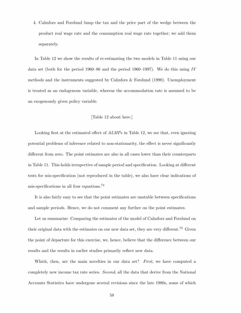
4. Calmfors and Forslund lump the tax and the price part of the wedge between the

product real wage rate and the consumption real wage rate together; we add them

separately.

In Table 12 we show the results of re-estimating the two models in Table 11 using our

data set (both for the period 1960–86 and the period 1960–1997). We do this using IV

methods and the instruments suggested by Calmfors & Forslund (1990). Unemployment

is treated as an endogenous variable, whereas the accommodation rate is assumed to be

an exogenously given policy variable.


Looking first at the estimated effect of ALMPs in Table 12, we see that, even ignoring

potential problems of inference related to non-stationarity, the effect is never significantly

different from zero. The point estimates are also in all cases lower than their counterparts

in Table 11. This holds irrespective of sample period and specification. Looking at different

tests for mis-specification (not reproduced in the table), we also have clear indications of

mis-specifications in all four equations.74

It is also fairly easy to see that the point estimates are unstable between specifications

and sample periods. Hence, we do not comment any further on the point estimates.

Let us summarise: Comparing the estimates of the model of Calmfors and Forslund on

their original data with the estimates on our new data set, they are very different.75 Given

the point of departure for this exercise, we, hence, believe that the difference between our

results and the results in earlier studies primarily reflect new data.

Which, then, are the main novelties in our data set? First, we have computed a

completely new income tax rate series. Second, all the data that derive from the National

Accounts Statistics have undergone several revisions since the late 1980s, some of which

58

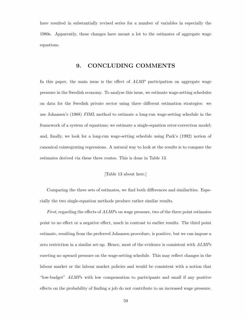
have resulted in substantially revised series for a number of variables in especially the

1980s. Apparently, these changes have meant a lot to the estimates of aggregate wage

equations.

9. CONCLUDING COMMENTS

In this paper, the main issue is the effect of ALMP participation on aggregate wage

pressure in the Swedish economy. To analyse this issue, we estimate wage-setting schedules

on data for the Swedish private sector using three different estimation strategies: we

use Johansen’s (1988) FIML method to estimate a long-run wage-setting schedule in the

framework of a system of equations; we estimate a single-equation error-correction model;

and, finally, we look for a long-run wage-setting schedule using Park’s (1992) notion of

canonical cointegrating regressions. A natural way to look at the results is to compare the

estimates derived via these three routes. This is done in Table 13.


Comparing the three sets of estimates, we find both differences and similarities. Espe-

cially the two single-equation methods produce rather similar results.

First, regarding the effects of ALMPs on wage pressure, two of the three point estimates

point to no effect or a negative effect, much in contrast to earlier results. The third point

estimate, resulting from the preferred Johansen procedure, is positive, but we can impose a

zero restriction in a similar set-up. Hence, most of the evidence is consistent with ALMPs

exerting no upward pressure on the wage-setting schedule. This may reflect changes in the

labour market or the labour market policies and would be consistent with a notion that

“low-budget” ALMPs with low compensation to participants and small if any positive

effects on the probability of finding a job do not contribute to an increased wage pressure.

59

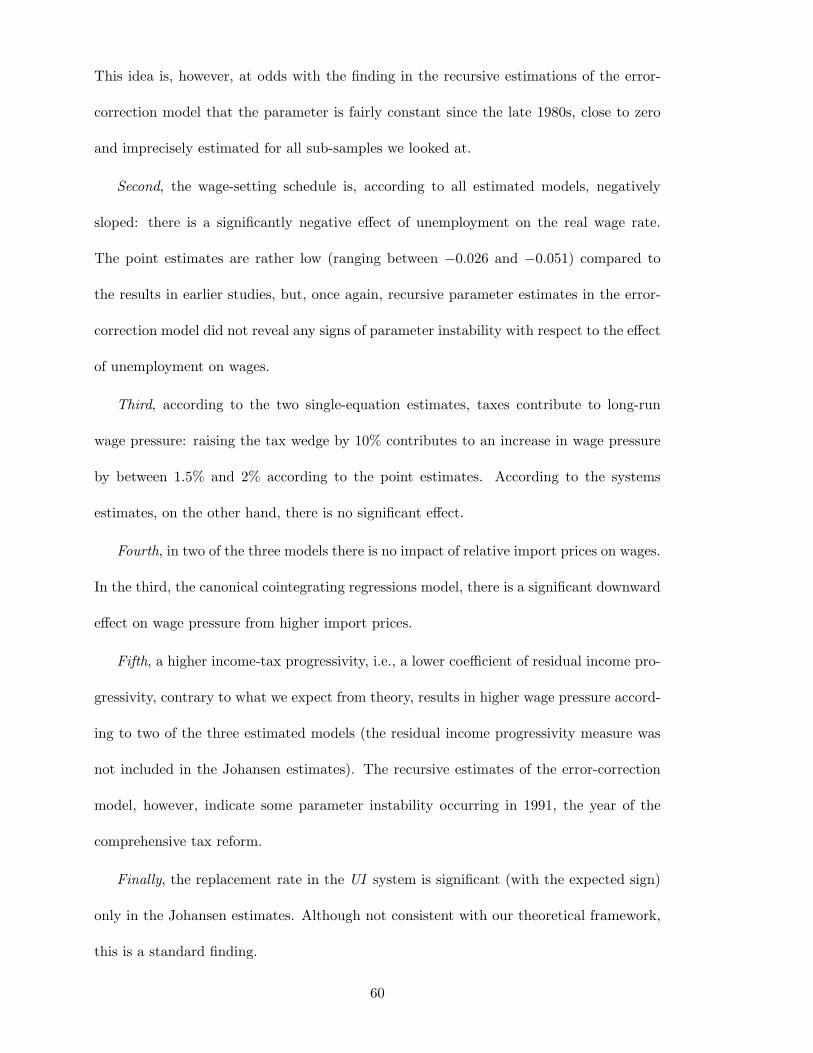
This idea is, however, at odds with the finding in the recursive estimations of the error-

correction model that the parameter is fairly constant since the late 1980s, close to zero

and imprecisely estimated for all sub-samples we looked at.

Second, the wage-setting schedule is, according to all estimated models, negatively

sloped: there is a significantly negative effect of unemployment on the real wage rate.

The point estimates are rather low (ranging between −0.026 and −0.051) compared to

the results in earlier studies, but, once again, recursive parameter estimates in the error-

correction model did not reveal any signs of parameter instability with respect to the effect

of unemployment on wages.

Third, according to the two single-equation estimates, taxes contribute to long-run

wage pressure: raising the tax wedge by 10% contributes to an increase in wage pressure

by between 1.5% and 2% according to the point estimates. According to the systems

estimates, on the other hand, there is no significant effect.

Fourth, in two of the three models there is no impact of relative import prices on wages.

In the third, the canonical cointegrating regressions model, there is a significant downward

effect on wage pressure from higher import prices.

Fifth, a higher income-tax progressivity, i.e., a lower coefficient of residual income pro-

gressivity, contrary to what we expect from theory, results in higher wage pressure accord-

ing to two of the three estimated models (the residual income progressivity measure was

not included in the Johansen estimates). The recursive estimates of the error-correction

model, however, indicate some parameter instability occurring in 1991, the year of the

comprehensive tax reform.

Finally, the replacement rate in the UI system is significant (with the expected sign)

only in the Johansen estimates. Although not consistent with our theoretical framework,

this is a standard finding.

60

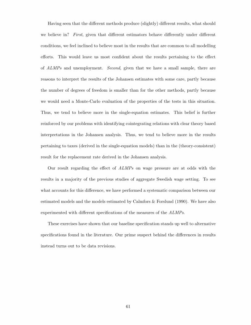
Having seen that the different methods produce (slightly) different results, what should

we believe in? First, given that different estimators behave differently under different

conditions, we feel inclined to believe most in the results that are common to all modelling

efforts. This would leave us most confident about the results pertaining to the effect

of ALMPs and unemployment. Second, given that we have a small sample, there are

reasons to interpret the results of the Johansen estimates with some care, partly because

the number of degrees of freedom is smaller than for the other methods, partly because

we would need a Monte-Carlo evaluation of the properties of the tests in this situation.

Thus, we tend to believe more in the single-equation estimates. This belief is further

reinforced by our problems with identifying cointegrating relations with clear theory based

interpretations in the Johansen analysis. Thus, we tend to believe more in the results

pertaining to taxes (derived in the single-equation models) than in the (theory-consistent)

result for the replacement rate derived in the Johansen analysis.

Our result regarding the effect of ALMPs on wage pressure are at odds with the

results in a majority of the previous studies of aggregate Swedish wage setting. To see

what accounts for this difference, we have performed a systematic comparison between our

estimated models and the models estimated by Calmfors & Forslund (1990). We have also

experimented with different specifications of the measures of the ALMPs.

These exercises have shown that our baseline specification stands up well to alternative

specifications found in the literature. Our prime suspect behind the differences in results

instead turns out to be data revisions.

61

NOTES

1Looking at the absolute value of the estimated effect.

2There are also some studies on micro data that point to no effects or wage moderating effects of ALMPs

(Edin et al. 1995, Forslund 1994). See also Raaum & Wulfsberg (1997) for an analysis with similar results

for Norway using micro data.

3In international comparisons, the sensitivity of Swedish wage setters to variations in the unemployment

rate has been high, see for example Layard et al. (1991) and the survey by Forslund (1997). The latter

also contains a general survey of studies of Swedish wage setting on aggregate data.

4This wedge reflects income taxes, payroll taxes and value-added taxes.

5Although it is hard to distinguish negative duration dependence from selection as the reason behind

the observed lower hazards to employment for the long-term unemployed.

6This aspect is closely related to the original raison d’etre for ALMPs put forward by Rehn and Meidner

in the 1950s.

7Direct displacement effects of ALMPs in the Swedish case are discussed in Gramlich & Ysander (1981),

Forslund & Krueger (1997), Forslund (1995), Sjostrand (1997), Lofgren & Wikstrom (1997) and Dahlberg

& Forslund (1999).

8There are some exceptions. Larsen (1997) deals with ALMPs as an instrument to maintain or increase

the average productivity of the pool of unemployed workers. Binder (1997) and Fukushima (1998) take

ALMPs as a skill up-grading device one step further by introducing heterogeneity in terms of skills. ALMPs

provide an opportunity for low-skill workers to upgrade their skills. Fukushima finds that in addition to

the two off-setting effects traced out in the basic model, there may be a “relative labour market tightness

effect” which tends to increase wage demands and unemployment, when ALMPs are targeted towards

unemployed low skilled workers.

9Homothetic preferences enables aggregation across consumers. Hence also foreign consumers are as-

sumed to have homothetic preferences.

10Ignoring value-added taxes for simplicity.

11We suppress physical capital to simplify the exposition. This can be justified either if labour and

capital are used in fixed proportions for technological reasons, or if the relative price of capital is fixed

(admittedly somewhat far-fetched). A second reason to exclude capital from the theoretical exposition is

that we believe that available measures of physical capital and capital prices are of such a poor quality that

62

we do not want to use them in the empirical analysis. Thus, as the primary objective of the theoretical

exposition is to lay a foundation for the empirical analysis, we concentrate on aspects we believe to be of

importance for the empirical work.

12See Layard & Nickell (1990) for a more detailed presentation of the basic model.

13Thus, we assume that the value of not reaching an agreement is zero for the firm.

14Qi = Yi/Ni, ωi = Wi (1 + t) /PiQi.

15This statement is, however, based on that the effect of the real producer wage on the labour demand

elasticity is not dominating the direct effect, as well as the indirect effects on the labour cost shares. Also,

recall that the WS-schedule is conditioned on the relative price of imports, the average and marginal tax

rates, and the real aggregate demand, which is the case throughout the section.

16The model used by Calmfors & Lang (1995) allows targeting of policy towards new entrants, but not

towards the truly long term unemployed, who are modelled as out of the labour force in their model.

17Note that a c < 1 is not necessary to generate the two off-setting effects.

18Such reasons include costs of adjustment and time aggregation, which we have not modelled explicitly.

19Some useful references are Johansen (1988), Banerjee et al. (1993), Hendry (1995) and Johansen (1995).

20Such as EViews, PcFiml, Rats and TSP.

21Exogeneity can mean a lot of things. Here it, somewhat loosely, refers to the following situation: In

the model yt = a0 +a1xt + εt, xt is said to be weakly exogenous with respect to the parameter a1 if correct

inference about it can be drawn without modelling xt.

22Given correctly specified dynamics, the methods also, obviously, provide information on the dynamics

of the wage-setting process.

23A more thorough data description is given in an appendix available on request.

24We use this variable instead of the product real wage for two reasons. First, we have an urgent need

to keep the number of variables down because of our wish to estimate a system. Second, several empirical

studies of Swedish wage setting have tested the implied restriction on the effect of productivity on wages

without rejecting it (see for example Forslund (1995); Rødseth & Nymoen (1999)).

25Numbers from reports N 1975:98, N1981:2, N 10 1985 and N 10 1997 from Statistics Sweden have

been chained. This procedure has been followed for all series based on the National Accounts. All data

for 1997 are taken from preliminary figures published by the National Institute for Economic Research

(Analysunderlag varen 1998).

26We use lower-case letters to denote logarithms of the corresponding variables.

63

27We are well aware that single-equation unit-root tests can at best be indicative, and we do not suggest

that certain variables “are”, for example, first-order integrated.

28Due to changes in both definitions and methods of measurement, there are breaks in the LFS unem-

ployment series. The present series is chained by multiplying the old series by the ratio between it and the

new one at common observations.

29Only those programme participants who are not included among the employed are, of course, added.

30We use the logarithmic transformation both because this potentially makes the normal distribution a

better approximation and, more fundamentally, because the log form is consistent with a hypothesis about

the marginal effect on wages from a rise in unemployment from 1% to 2% being larger than a rise from 9%

to 10%.

31This factor equals 1 + t.

32The indirect tax factor equals 1 + V AT.

33As computed from the National Accounts Statistics.

34Details are given in an appendix available on request.

35There could, in principle, also be a third choice, if one is willing to assume weak exogeneity of some

variables already at the outset. Then one would have to decide which variables could be treated as weakly

exogenous (non-modelled) in the system. We did some experimentation along these lines, but almost

always ended up with systems with badly behaved residuals.

36We denote the labour share by w − q rather than by w − pp − q.

37This is, e.g., discussed in Layard et al. (1991).

38The maximum number of variables followed because we decided, a priori, to estimate a baseline system

with two lags. All estimations have been performed in PcFiml 9.2, see Doornik & Hendry (1997).

39P-values for autocorrelations of order 1, 1-2 and 1-3 are .17, .69 and .24, respectively. We would like

to point out that this has been achieved without any use of dummies to “clean” the residuals.

40To see this, define the “long run” as a situation in which ∆yt = vt = 0. Then clearly P0y = 0 defines

a long-run relation between the variables, where the coefficients are given by P0.

41This is almost generically true of aggregate wage-setting schedules in bargaining models, see Bean

(1994) and Manning (1993).

42Leaving the trend out.

43To see this, notice that the product of the β′ matrix and the y vector is a (3× 1) vector, the elements

of which are three linear combinations of the elements of y. Each row of α translates these into a ∆yi.

64

44It is important to remember that weak exogeneity is defined relative to the system at hand.

45The normalisation of the cointegrating vectors is arbitrary.

46The wage elasticity of demand can be decomposed into a substitution effect and an “output” effect.

In our case it can be written εN = σ(1− νN ) + ηνN/(1− dmu

dP

P

mu), where σ is the elasticity of substitution

between capital and labour, νN the labour share of costs and mu the ratio between price and cost (the

mark-up). The argument in the text follows if the price elasticity of the mark-up factor and the labour

share of costs do not change “too much”.

47At least the authors have had a hard time coming up with a mechanism with this effect.

48We cannot, however, rule out that the effect equals zero, see Section 6.1.5.

49That is, effects on the wage costs, the implication of which is that taxes in the long run are borne by

wage earners.

50This equation directly corresponds to Equation 17 in Section 6.

51Notice, however, that, according to our theoretical framework, this effect works through changes in

the elasticity of product demand.

52It is actually reasonable to label it a demand shock in this model, since our tests indicate that unem-

ployment is weakly exogenous in the system. One should, however, keep in mind that we are talking about

long-run relationships.

53The restrictions on the other long-run equations are primarily motivated by theoretical considerations.

54The point estimates are around -0.3 for programmes and above 1.0 for the replacement rate.

55That is, we can trace the effects of changes in unemployment on wage setting without modelling the

unemployment rate. See the discussion in Bean (1994).

56The critical values for the significance tests for the lagged levels variables are not given by the t-

distribution; the Dickey-Fuller distribution should be used instead, see Kremers et al. (1992).

57We have tested and not rejected nominal homogeneity both in the short and in the long run by using

the change in the nominal wage cost as the left-hand side variable and the producer price on the right-hand

side. Thus, we start in a real model.

58The instruments used in the IV estimation were the logged world market oil price in t and t − 1; the

long-run US real interest rate in t an t−1; ∆qt−1, ∆ut−1; ∆γt−1, ∆θt−1; ∆ript−1; ∆(pI −p)t−1 and ∆ρt−1.

∆qt, ∆γt, ∆ript and ∆(pI − p)t were treated as endogenous, given the results of the exogeneity tests in

the systems analysis. The diagnostic tests used were tests for first- and second-order autocorrelation in the

residuals (AR(1–2)), ARCH (1), residual normality and a RESET test for heteroskedasticity. The Sargan

65

test for instrument validity was passed at the 10% level.

59It is often considered to be a stylised fact that wage costs in the long run are unit elastic with respect to

labour productivity. If that is the case, the wage share and employment will be independent of productivity

developments in the long run. This is, however, a property of the equilibrium of the whole system and

not only of the wage-setting schedule. Nevertheless, we will test the restriction that also the wage-setting

schedule is unit elastic with respect to labour productivity. It is hard to find good theoretical reasons for

this restriction, but we feel the fact that it has been tested without rejection in a number of earlier studies

(for example Rødseth & Nymoen (1999) and Forslund (1995)) is a good enough reason. This restriction

was also imposed rather than tested in our systems analysis.

60The test used was a Wald test. The p-values were 0.37 (IV ) and 0.22 (OLS).

61χ2(4) = 34.843[0.0000]∗∗ in the OLS model and χ2(4) = 25.714[0.0000]∗∗ in the IV model.

62The estimated effects of ALMPs and the replacement rate are, for example, both smaller and statist-

ically insignificant in the IV estimation. The sign of the estimated effect of the replacement rate is even

negative.

63OLS results, presented for the sake of comparison, are given in Table 7.

64As ALMPs are not included in the parsimonious model, there are no recursive parameter estimates

plotted for this variable. Looking instead at recursive estimates of the parameters of the full model, the

effect of ALMPs is estimated to be close to zero in all sub-samples from 1988 an onwards. It is also very

imprecisely estimated. Thus, there are no signs of a significant change in this (non-)effect.

65The test statistics are not distributed according to the t-distribution, because the variables, according

to our previous tests, are first-order integrated. See footnote 56.

66To see the second property, notice that the partial derivative of the wage share with respect to the

programme participation rate equals (a22 +a2

3)/(u+ r). Thus, the partial effect of programme participation

equals zero in the case referred to in the text.

67Notice, however, that critical values should not be taken from the usual distributions, see footnote on

page 65.

68Raising the accommodation rate from 30 per cent to 50 per cent at a given level of “total unemploy-

ment” would raise the wage pressure by about 1.5 per cent.

69With the exception of the estimated effect of income tax progressivity, which behaves in the same way

as in the baseline model; the estimated effect of the lagged wage share is also somewhat unstable.

70This is a necessary but not sufficient condition for encompassing in linear regression models, see Hendry

66

(1995), ch. 14.

71The Gauss code, implementing CCR, was most kindly supplied by Per Jansson, Bank of Sweden.

72Unfortunately, the original data used by Calmfors and Forslund are not available; the main differences

between our data and theirs derive from revisions in the National Accounts Statistics and new computations

of income tax rates. Given their data, we could have estimated our models on their original data to check

for differences.

73R is the fraction of the labour force in ALMPs.

74An example is that the Durbin-Watson statistic in Equation 1a equals 0.66, that the Sargan test rejects

instrument validity and that there is significant ARCH 1 and heteroskedasticity in the same equation.

75We have not used exactly the same estimation technique as Calmfors and Forslund (they used an

iterative three-stage least squares method), so this could still make a small difference.

67

ACKNOWLEDGEMENTS

We are grateful to Per Jansson, Bank of Sweden, Kerstin Johansson, Institute for Labour

Market Policy Evaluation (IFAU), Ragnar Nymoen, University of Oslo and seminar parti-

cipants at IFAU, Bank of Sweden and Vaxjo University for comments on earlier versions

of the paper. The usual caveat applies.

REFERENCES

Ackum Agell, S. (1996), ‘Arbetslosas sokaktivitet, Search activity of the unemployed, (in

Swedish)’, Appendix to SOU 1996:34, Aktiv Arbetsmarknadspolitik, Active labour

market policies, (in Swedish), Stockholm.

Banerjee, A., Dolado, J. J., Galbraith, J. W. & Hendry, D. F. (1993), Co-Integration, Error

Correction and the Econometric Analysis of Non-Stationary Data, Oxford University

Press, Oxford.

Bean, C., Layard, R. & Nickell, S. (1986), ‘The rise in unemployment: A multi-country

study’, Economica 53, S1–S22.

Bean, C. (1994), ‘European unemployment: A survey’, Journal of Economic Literature

XXXII, 573–619.

Binder, M. (1997), Aktiv Arbejdsmarkedspolitik og Økonomisk Marginalisering—En

Teoretisk Analyse af den Aktive ArbejdsmarkedsPolitiks Langsigtede Virkninger

pa Ledighedens Størrelse og Fordeling, Active labour market policies and

marginalisation—A theoretical analysis of the long-run effects of active labour mar-

ket policies on the size and distribution of unemployment, (in Danish), PhD thesis,

Department of Economics, University of Copenhagen.

68

Calmfors, L. & Forslund, A. (1990), Wage formation in sweden, in L. Calmfors, ed., ‘Wage

Formation and Macroeconomic Policy in the Nordic Countries’, SNS and Oxford

University Press, Stockholm.

Calmfors, L. & Forslund, A. (1991), ‘Real-wage determination and labour market policies:

The Swedish experience’, The Economic Journal 101, 1130–1148.

Calmfors, L. & Lang, H. (1995), ‘Macroeconomic effects of active labour market pro-

grammes in a union wage-setting model’, The Economic Journal 105, 601–619.

Calmfors, L. & Nymoen, R. (1990), ‘Nordic employment’, Economic Policy 5, 397–448.

Calmfors, L. (1994), ‘Active labour market policy and unemployment. a framework for the

analysis of crucial design features’, OECD Economic Studies 22, 7–47.

Dahlberg, M. & Forslund, A. (1999), Direct displacement effects of labour market pro-

grammes: The case of sweden, Working Paper 1999:7, Office of Labour Market Policy

Evaluation, Uppsala.

Doornik, J. A. & Hendry, D. F. (1997), Modelling Dynamic Systems Using PcFiml 9.0 for

Windows, International Thomson Business Press, London.

Edin, P.-A., Holmlund, B. & Ostros, T. (1995), Wage behaviour and labour market pro-

grammes in sweden: Evidence from micro data, in Tachibanaki, ed., ‘Labour Market

and Macroeconomic Performance in Europe, Japan and the US’, Macmillan, London.

Edin, P.-A. & Holmlund, B. (1991), Unemployment, vacancies and labour market pro-

grammes: Swedish evidence, in F. Padoa-Schioppa, ed., ‘Mismatch and Labour Mo-

bility’, Cambridge University Press, Cambridge.

69

Edin, P.-A. (1989), Individual Consequences of Plant Closures, Phd thesis, Department of

Economics, Uppsala University.

Engle, R. & Granger, C. (1987), ‘Co-integration and error correction: Representation,

estimation, and testing’, Econometrica 55, 251–276.

Forslund, A. & Krueger, A. B. (1997), An evaluation of the Swedish active labor market

policy: New and received wisdom, in R. B. Freeman, R. Topel & B. Swedenborg,

eds, ‘The Welfare State in Transition. Reforming the Swedish Model’, University of

Chicago Press, Chicago.

Forslund, A. & Risager, O. (1994), Wages in sweden. new and old results, Memo 1994-22,

University of Aarhus, Institute of Economics.

Forslund, A. (1992), ‘Arbetsloshet och arbetsmarknadspolitik, Unemployment and labour

market policies, (in Swedish)’, Appendix 7 to the Medium Term Survey of the Swedish

Economy 1992, Ministry of Finance, Stockholm.

Forslund, A. (1994), ‘Wage setting at the firm level—insider versus outsider forces’, Oxford

Economic Papers 46, 245–261.

Forslund, A. (1995), ‘Unemployment—is sweden still different?’, Swedish Economic policy

Review 2(1), 17–58.

Forslund, A. (1997), ‘Lonebildningen och arbetsmarknadens funktionssatt, Wage forma-

tion and the functioning of the labour market, (in Swedish)’, Appendix 1 to SOU

1997:164, Ministry of Labour, Stockholm.

Fukushima, Y. (1998), Active labour market programmes and unemployment in a dual

labour market, Research Paper 1998:2, Department of Economics, Stockholm Uni-

versity.

70

Gramlich, E. M. & Ysander, B.-C. (1981), Relief work and grant displacement in sweden, in

G. Eliasson, B. Holmlund & F. P. Stafford, eds, ‘Studies in Labor Market Behavior:

Sweden and the United States’, The Industrial Institute for Economic and Social

Research, Stockholm.

Hendry, D. F. & Doornik, J. A. (1996), Empirical Econometric Modelling Using PcGive

9.0 for Windows, International Thomson Business Press, London.

Hendry, D. F. (1995), Dynamic Econometrics, Oxford University Press, Oxford.

Holmlund, B. & Kolm, A.-S. (1995), ‘Progressive taxation, wage setting and unemploy-

ment: Theory and Swedish evidence’, Swedish Economic Policy Review 2, 425–460.

Holmlund, B. & Linden, J. (1993), ‘Job matching, temporary public employment and

equilibrium unemployment’, Journal of Public Economics 51, 329–343.

Holmlund, B. (1989), Wages and employment in unionized economies: Theory and evid-

ence, in B. Holmlund, K.-G. Lofgren & L. Engstrom, eds, ‘Trade Unions, Employ-

ment, and Unemployment Duration’, Oxford University Press, Oxford.

Holmlund, B. (1990), ‘Svensk lonebildning—teori, empiri, politik, Swedish wage

formation—theory, evidence, policy, (in Swedish)’, Appendix 24 to the Medium Term

Survey of the Swedish Economy 1990, Ministry of Finance, Stockholm.

Johansen, S. (1988), ‘Statistical analysis of cointegrating vectors’, Journal of Economic

Dynamics and Control 12, 231–254.

Johansen, S. (1995), Likelihood-Based Inference in Cointegrated Vector Autoregressive

Models, Oxford University Press, Oxford.

71

Johansson, S., Lundborg, P. & Zetterberg, J. (1999), Massarbetsloshetens Karaktar, The

character of mass unemployment, (in Swedish), The Trade Union Institute for Eco-

nomic Research, Stockholm.

Kremers, J. J. M., Ericsson, N. & Dolado, J. (1992), ‘The power of cointegration tests’,

Oxford Bulletin of Economics and Statistics 54, 325–348.

Larsen, B. (1997), Active labour market programmes and loss of skill. mimeo.

Layard, R., Nickell, S. & Jackman, R. (1991), Unemployment—Macroeconomic Perform-

ance and the Labour Market, Oxford University Press, Oxford.

Layard, R. & Nickell, S. (1990), ‘Is unemployment lower if unions bargain over employ-

ment?’, Quarterly Journal of Economics 105, 773–787.

Lockwood, B. & Manning, A. (1993), ‘Wage setting and the tax system: Theory and

evidence for the united kingdom’, Journal of public Economics 52, 1–29.

Lofgren, K.-G. & Wikstrom, M. (1991), ‘Lonebildning och arbetsmarknadspolitik, Wage

formation and labour market policies, (in Swedish)’, Appendix to Ds 1991:53 Arbets-

marknad och arbetsmarknadspolitik, The labour market and labour market policies,

(in Swedish), Ministry of Labour, Stockholm.

Lofgren, K.-G. & Wikstrom, M. (1997), ‘Undantrangningseffekter av arbetsmarknad-

spolitik. Kommentarer till Forslund-Sjostrand kontroversen, Displacement effects

of labour market policies. Comments to the Forslund-Sjostrand controversy, (in

Swedish)’, Arbetsmarknad & Arbetsliv 3, 211–223.

LO (1951), Fackforeningsrorelsen och den fulla sysselsattningen, The trade union move-

ment and full employment, (in Swedish), LO, Stockholm.

72

Manning, A. (1992), ‘Multiple equilibria in the british labour market’, European Economic

Review 36, 1333–1365.

Manning, A. (1993), ‘Wage bargaining and the phillips curve: The identification and

specification of aggregate wage equations’, Economic Journal 103, 98–118.

Newell, A. & Symons, J. (1987), ‘Corporatism, laissez-faire and the rise in unemployment’,

European Economic Review 31, 567–614.

Park, J. Y. (1992), ‘Canonical cointegrating regressions’, Econometrica 60, 119–143.

Raaum, O. & Wulfsberg, F. (1997), Unemployment, labour market programmes and wages

in norway, Arbeidsnotater 11, Norges Bank.

Richardson, J. (1997), Can active labour market policy work?—some theoretical consid-

erations, Discussion Paper 331, Centre For Economic Preformance, London School of

Economics.

Rødseth, A. & Nymoen, R. (1999), Nordic wage formation and unemployment seven years

later, Memorandum 10/99, Department of Economics, University of Oslo.

Sjostrand, K.-M. (1997), Nagra kommentarer till Anders Forslunds rapport ’Direkta un-

dantrangningseffekter av arbetsmarknadspolitiska atgarder’, Some comments to An-

ders Forslunds report ’Direct displacement effects of labour market policies’, (in

Swedish). Mimeo, National Labour Market Board, Stockholm.

73

LIST OF FIGURES

1 Employment and wage determination . . . . . . . . . . . . . . . . . . . . . . 752 Labour market flows . . . . . . . . . . . . . . . . . . . . . . . . . . . . . . . 763 Log labour’s share of value added 1960–97 . . . . . . . . . . . . . . . . . . . 774 Log unemployment 1960–97 . . . . . . . . . . . . . . . . . . . . . . . . . . . 785 Log accommodation ratio 1960–1997 . . . . . . . . . . . . . . . . . . . . . . 796 The log of the tax wedge 1960–97 . . . . . . . . . . . . . . . . . . . . . . . . 807 Log residual income progressivity 1960–1997 . . . . . . . . . . . . . . . . . . 818 Log relative price of imports . . . . . . . . . . . . . . . . . . . . . . . . . . . 829 Log replacement rate in the unemployment insurance system . . . . . . . . 8310 Unrestricted cointegrating combinations . . . . . . . . . . . . . . . . . . . . 8411 Restricted cointegrating combinations . . . . . . . . . . . . . . . . . . . . . 8512 Actual and fitted values and scaled residuals in the dynamic system . . . . 8613 Actual and fitted values, scaled residuals, cross plot of actual and fitted

values, scaled residuals and residual correlogram . . . . . . . . . . . . . . . 8714 Recursive parameter estimates . . . . . . . . . . . . . . . . . . . . . . . . . 88

74

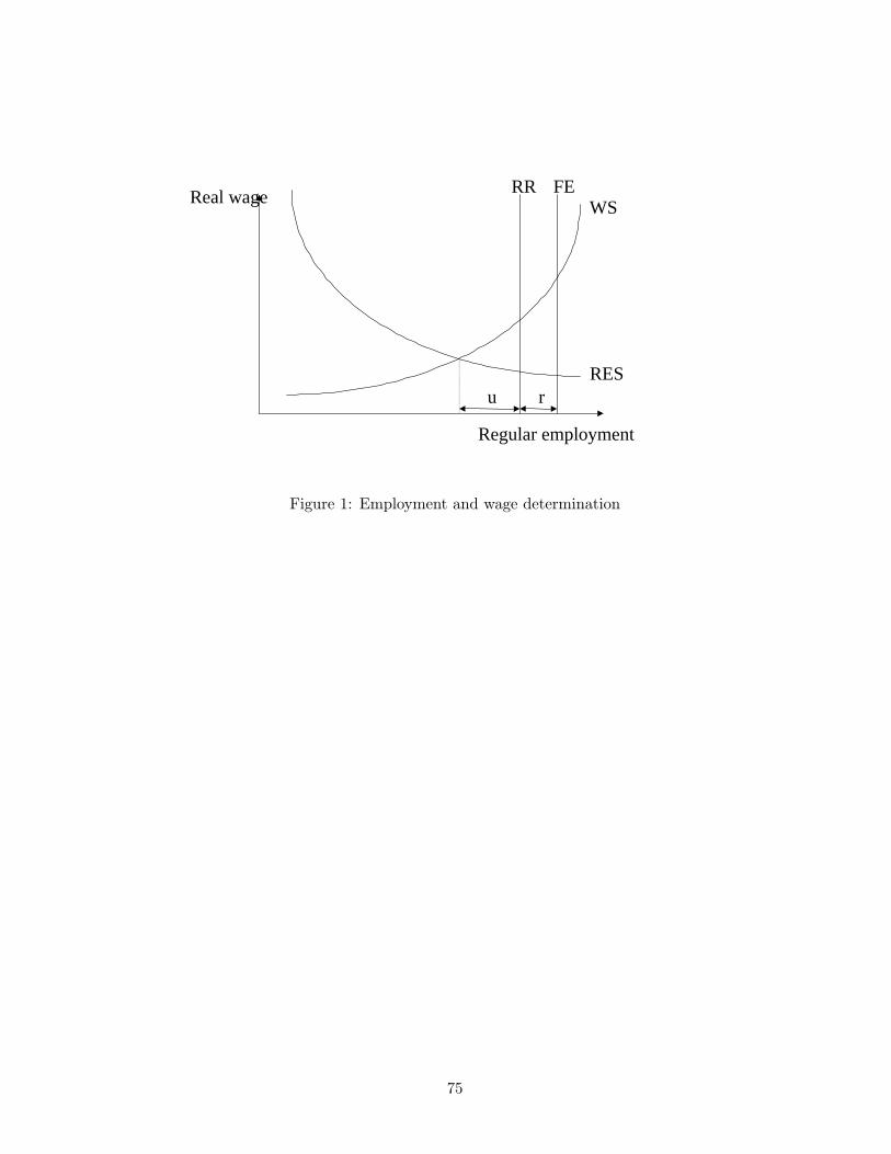
RES

WS

Regular employment

Real wageFERR

u r

Figure 1: Employment and wage determination

75

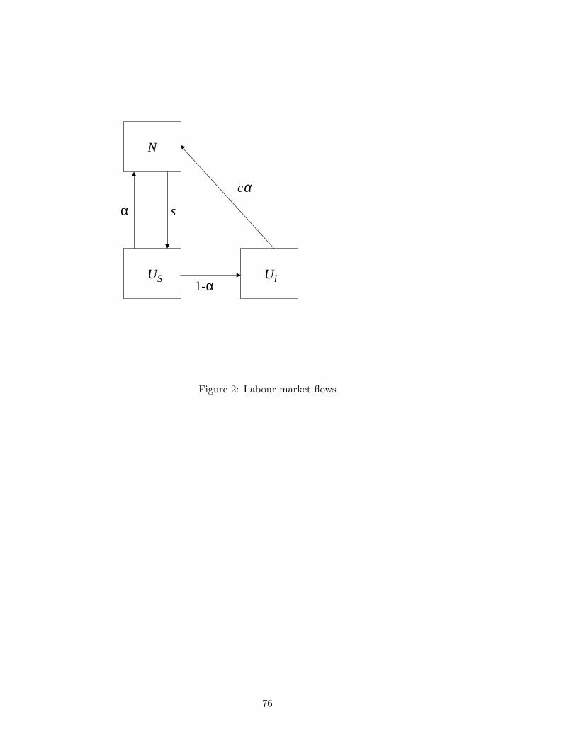
U U

N

S l

sα

1-α

cα

Figure 2: Labour market flows

76

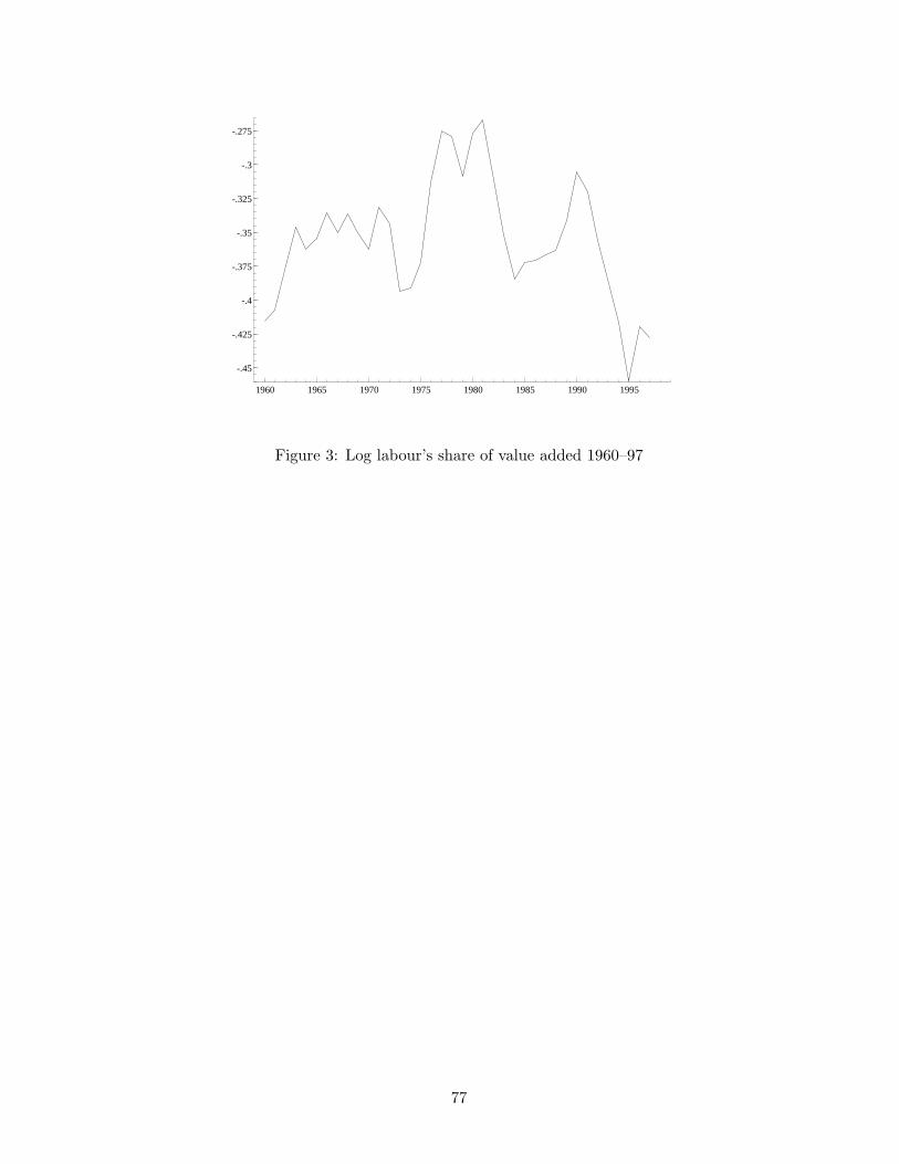
1960 1965 1970 1975 1980 1985 1990 1995

-.45

-.425

-.4

-.375

-.35

-.325

-.3

-.275

Figure 3: Log labour’s share of value added 1960–97

77

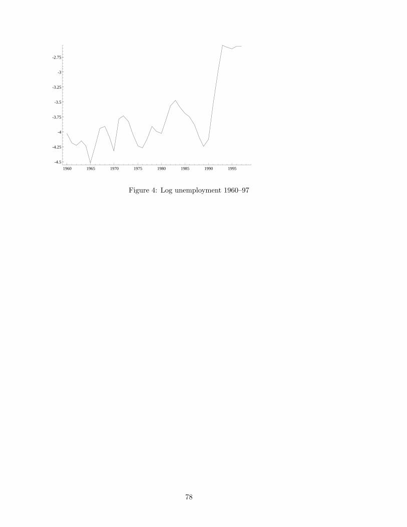
1960 1965 1970 1975 1980 1985 1990 1995

-4.5

-4.25

-4

-3.75

-3.5

-3.25

-3

-2.75

Figure 4: Log unemployment 1960–97

78

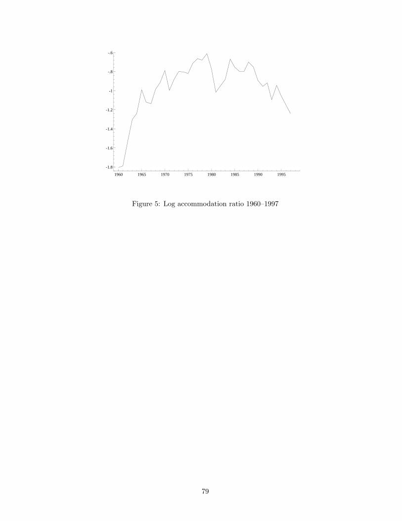
1960 1965 1970 1975 1980 1985 1990 1995

-1.8

-1.6

-1.4

-1.2

-1

-.8

-.6

Figure 5: Log accommodation ratio 1960–1997

79

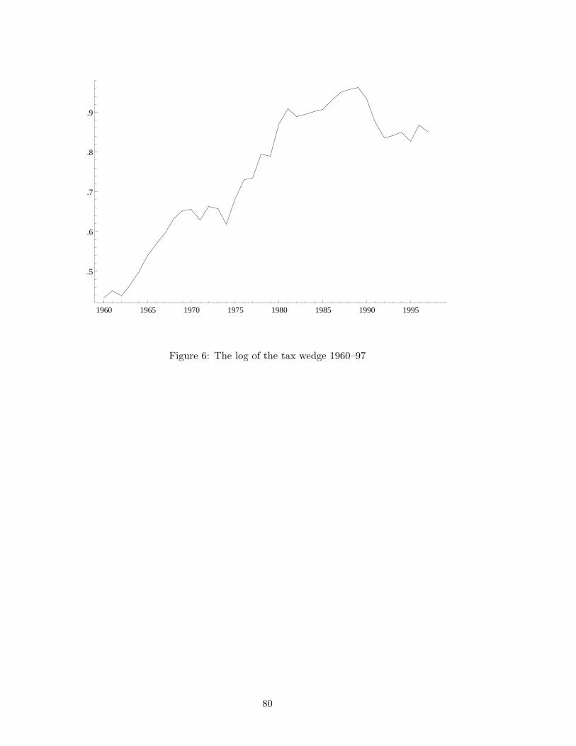
1960 1965 1970 1975 1980 1985 1990 1995

.5

.6

.7

.8

.9

Figure 6: The log of the tax wedge 1960–97

80

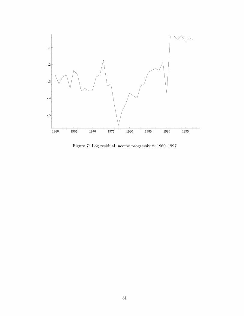
1960 1965 1970 1975 1980 1985 1990 1995

-.5

-.4

-.3

-.2

-.1

Figure 7: Log residual income progressivity 1960–1997

81

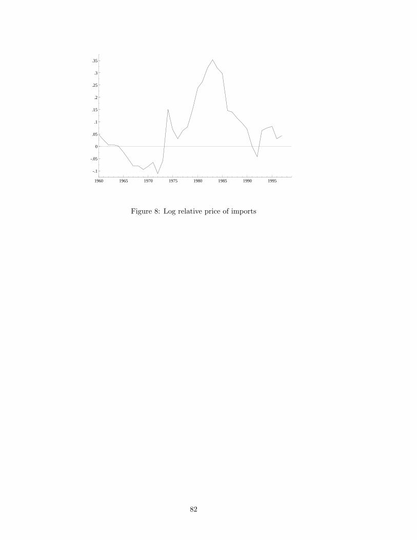
1960 1965 1970 1975 1980 1985 1990 1995

-.1

-.05

0

.05

.1

.15

.2

.25

.3

.35

Figure 8: Log relative price of imports

82

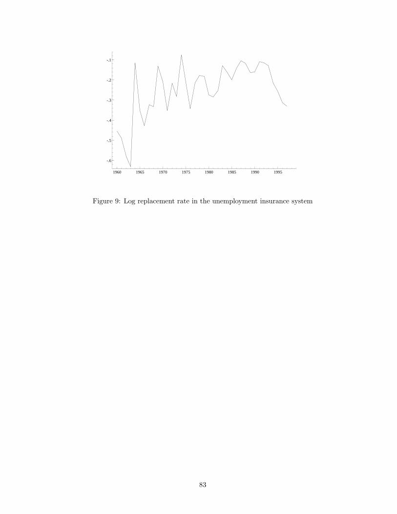
1960 1965 1970 1975 1980 1985 1990 1995

-.6

-.5

-.4

-.3

-.2

-.1

Figure 9: Log replacement rate in the unemployment insurance system

83

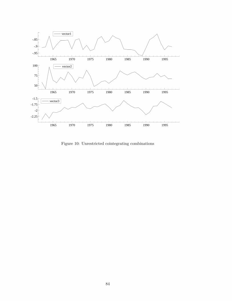
1965 1970 1975 1980 1985 1990 1995

-.95

-.9

-.85

vector1

1965 1970 1975 1980 1985 1990 1995

50

75

100 vector2

1965 1970 1975 1980 1985 1990 1995

-2.25

-2

-1.75

-1.5vector3

Figure 10: Unrestricted cointegrating combinations

84

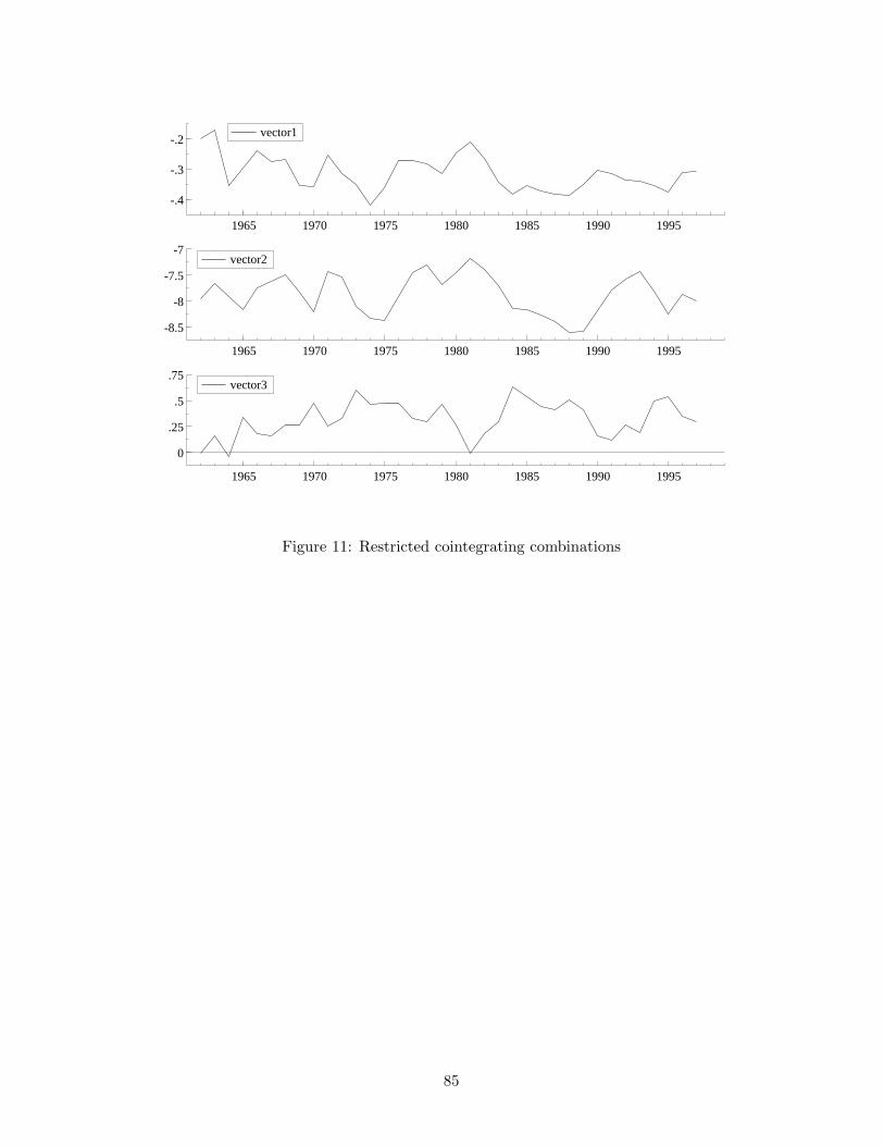
1965 1970 1975 1980 1985 1990 1995

-.4

-.3

-.2vector1

1965 1970 1975 1980 1985 1990 1995

-8.5

-8

-7.5

-7vector2

1965 1970 1975 1980 1985 1990 1995

0

.25

.5

.75vector3

Figure 11: Restricted cointegrating combinations

85

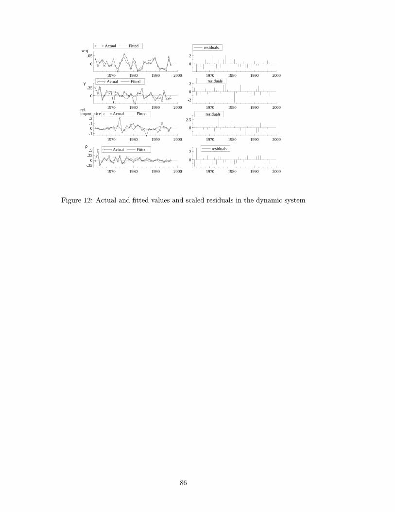
1970 1980 1990 2000

0

.05

rel.import price

ρ

γ

w-qActual Fitted

1970 1980 1990 2000

0

2

residuals

1970 1980 1990 2000

0

.25

Actual Fitted

1970 1980 1990 2000

-2

0

2residuals

1970 1980 1990 2000

-.10

.1

.2Actual Fitted

1970 1980 1990 2000

0

2.5residuals

1970 1980 1990 2000

-.250

.25.5 Actual Fitted

1970 1980 1990 2000

0

2residuals

Figure 12: Actual and fitted values and scaled residuals in the dynamic system

86

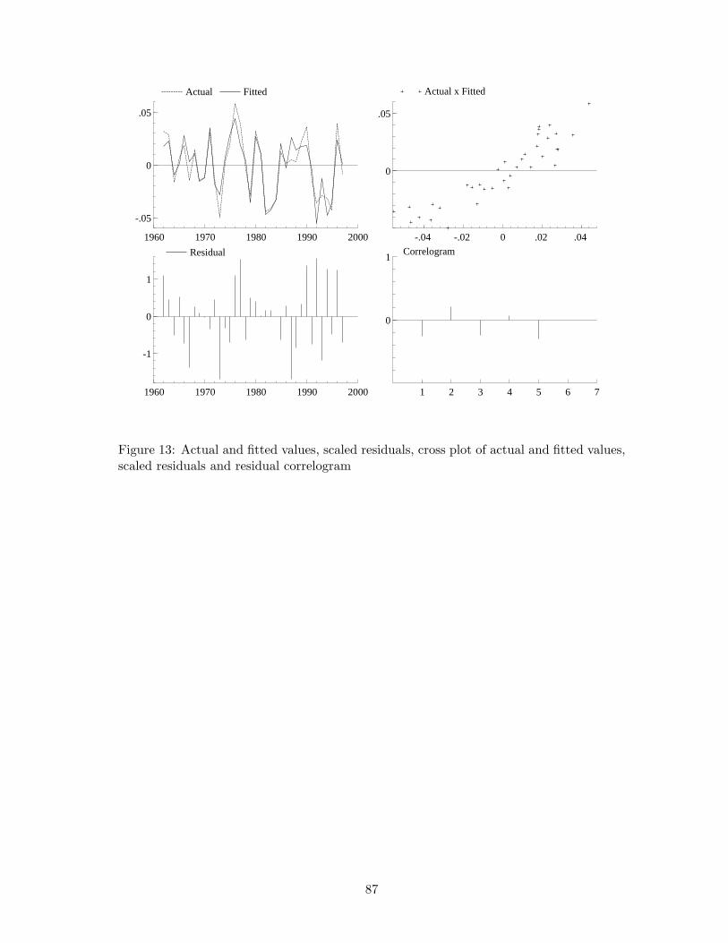
1960 1970 1980 1990 2000

-.05

0

.05

Actual Fitted

-.04 -.02 0 .02 .04

0

.05

Actual x Fitted

1960 1970 1980 1990 2000

-1

0

1

Residual

1 2 3 4 5 6 7

0

1Correlogram

Figure 13: Actual and fitted values, scaled residuals, cross plot of actual and fitted values,scaled residuals and residual correlogram

87

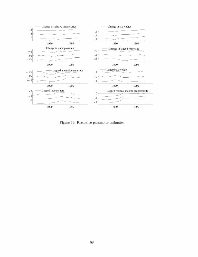
1990 1995

.1

.2

.3Change in relative import price

1990 1995

.2

.4

.6

Change in tax wedge

1990 1995

.025.05

.075

Change in unemployment

1990 1995

.25.5

.75Change in lagged real wage

1990 1995

-.075-.05

-.025Lagged unemployment rate

1990 1995

.1

.15

.2Lagged tax wedge

1990 1995

-1

-.75

-.5 Lagged labour share

1990 1995

-.2

-.1

0Lagged residual income progressivity

Figure 14: Recursive parameter estimates

88

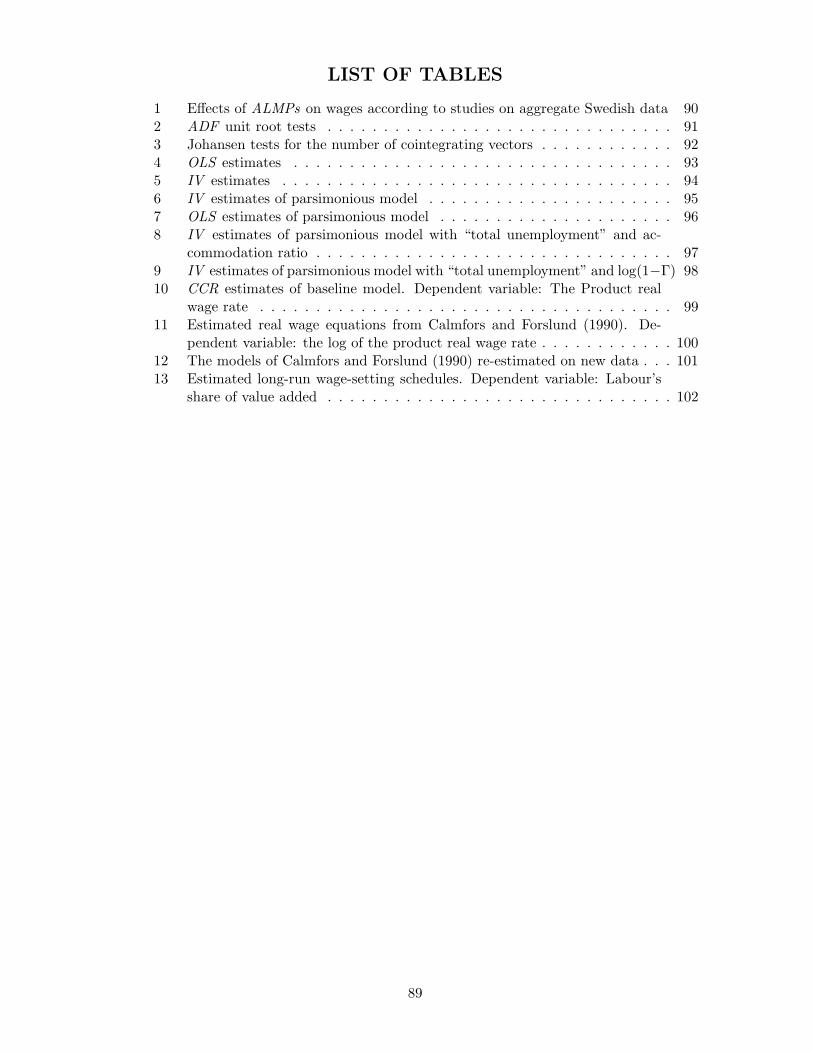
LIST OF TABLES

1 Effects of ALMPs on wages according to studies on aggregate Swedish data 902 ADF unit root tests . . . . . . . . . . . . . . . . . . . . . . . . . . . . . . . 913 Johansen tests for the number of cointegrating vectors . . . . . . . . . . . . 924 OLS estimates . . . . . . . . . . . . . . . . . . . . . . . . . . . . . . . . . . 935 IV estimates . . . . . . . . . . . . . . . . . . . . . . . . . . . . . . . . . . . 946 IV estimates of parsimonious model . . . . . . . . . . . . . . . . . . . . . . 957 OLS estimates of parsimonious model . . . . . . . . . . . . . . . . . . . . . 968 IV estimates of parsimonious model with “total unemployment” and ac-

commodation ratio . . . . . . . . . . . . . . . . . . . . . . . . . . . . . . . . 979 IV estimates of parsimonious model with “total unemployment” and log(1−Γ) 9810 CCR estimates of baseline model. Dependent variable: The Product real

wage rate . . . . . . . . . . . . . . . . . . . . . . . . . . . . . . . . . . . . . 9911 Estimated real wage equations from Calmfors and Forslund (1990). De-

pendent variable: the log of the product real wage rate . . . . . . . . . . . . 10012 The models of Calmfors and Forslund (1990) re-estimated on new data . . . 10113 Estimated long-run wage-setting schedules. Dependent variable: Labour’s

share of value added . . . . . . . . . . . . . . . . . . . . . . . . . . . . . . . 102

89

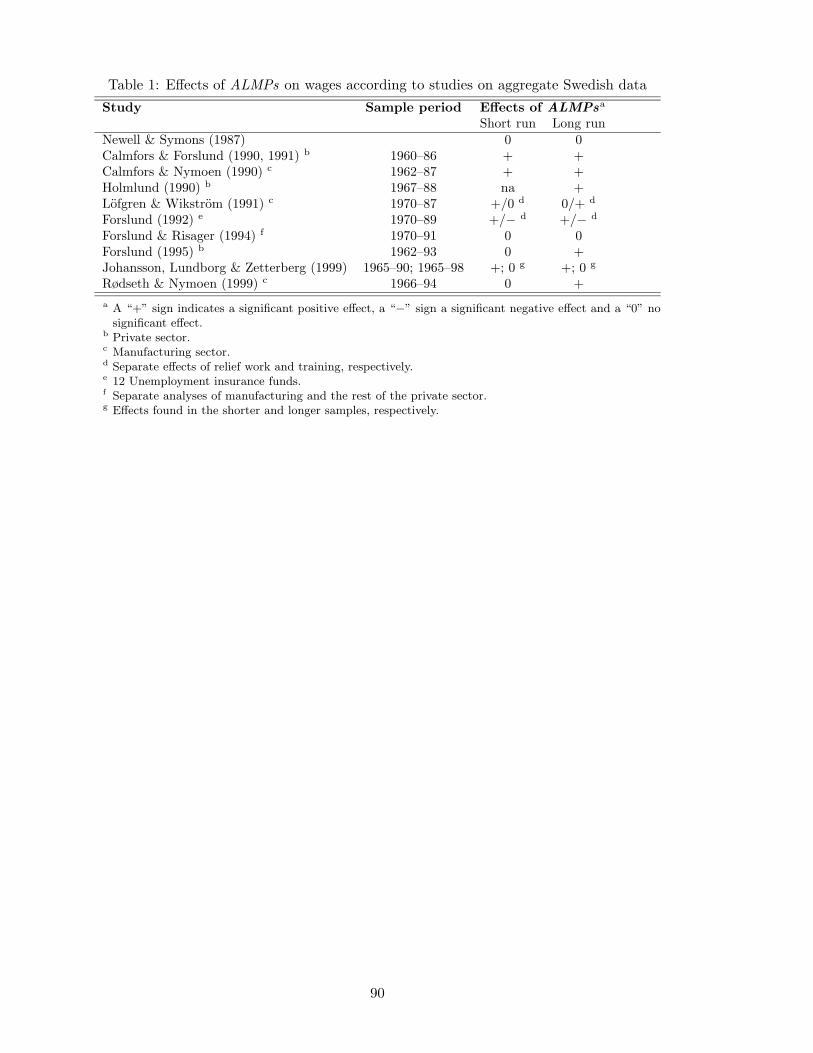
Table 1: Effects of ALMPs on wages according to studies on aggregate Swedish data

Study Sample period Effects of ALMPsa

Short run Long runNewell & Symons (1987) 0 0Calmfors & Forslund (1990, 1991) b 1960–86 + +Calmfors & Nymoen (1990) c 1962–87 + +Holmlund (1990) b 1967–88 na +Lofgren & Wikstrom (1991) c 1970–87 +/0 d 0/+ d

Forslund (1992) e 1970–89 +/− d +/− d

Forslund & Risager (1994) f 1970–91 0 0Forslund (1995) b 1962–93 0 +Johansson, Lundborg & Zetterberg (1999) 1965–90; 1965–98 +; 0 g +; 0 g

Rødseth & Nymoen (1999) c 1966–94 0 +

a A “+” sign indicates a significant positive effect, a “−” sign a significant negative effect and a “0” nosignificant effect.

b Private sector.c Manufacturing sector.d Separate effects of relief work and training, respectively.e 12 Unemployment insurance funds.f Separate analyses of manufacturing and the rest of the private sector.g Effects found in the shorter and longer samples, respectively.

90

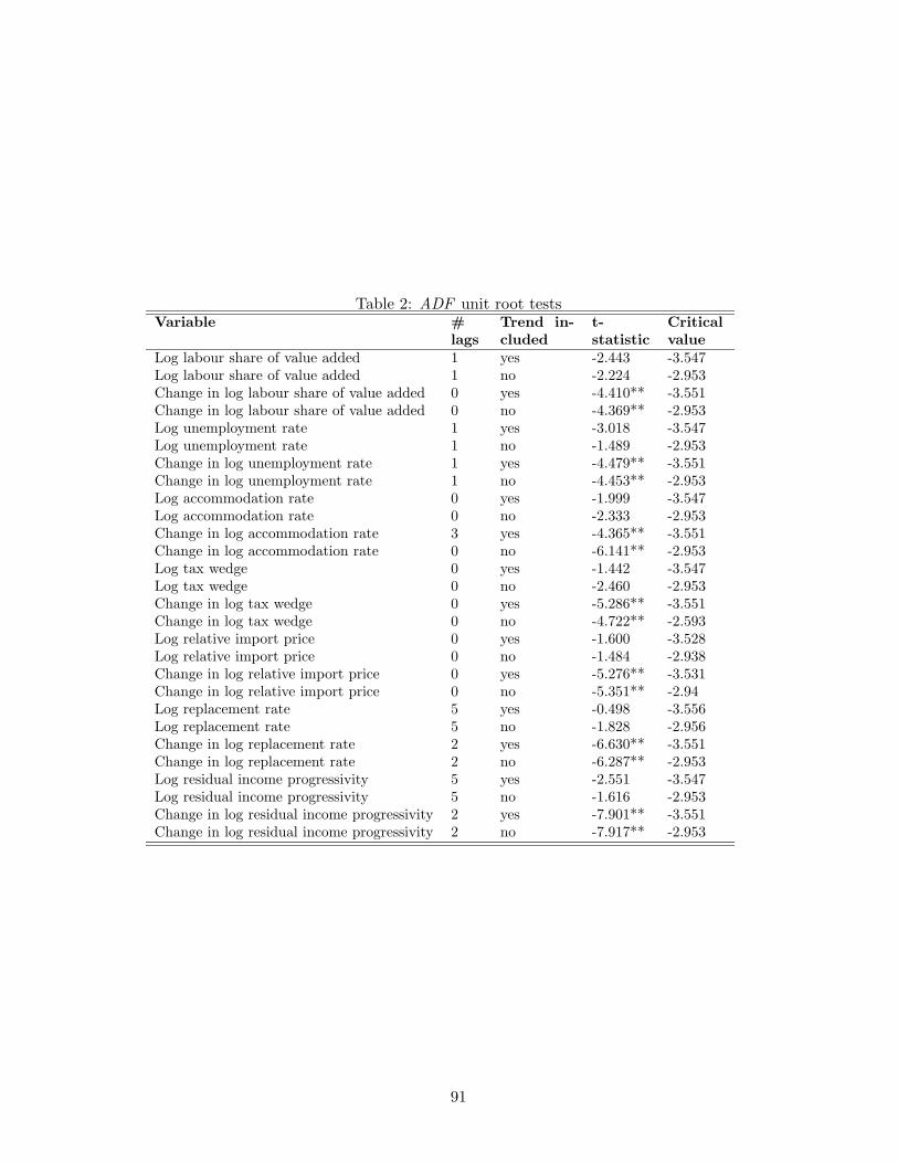
Table 2: ADF unit root testsVariable #

lags

Trend in-

cluded

t-

statistic

Critical

value

Log labour share of value added 1 yes -2.443 -3.547Log labour share of value added 1 no -2.224 -2.953Change in log labour share of value added 0 yes -4.410** -3.551Change in log labour share of value added 0 no -4.369** -2.953Log unemployment rate 1 yes -3.018 -3.547Log unemployment rate 1 no -1.489 -2.953Change in log unemployment rate 1 yes -4.479** -3.551Change in log unemployment rate 1 no -4.453** -2.953Log accommodation rate 0 yes -1.999 -3.547Log accommodation rate 0 no -2.333 -2.953Change in log accommodation rate 3 yes -4.365** -3.551Change in log accommodation rate 0 no -6.141** -2.953Log tax wedge 0 yes -1.442 -3.547Log tax wedge 0 no -2.460 -2.953Change in log tax wedge 0 yes -5.286** -3.551Change in log tax wedge 0 no -4.722** -2.593Log relative import price 0 yes -1.600 -3.528Log relative import price 0 no -1.484 -2.938Change in log relative import price 0 yes -5.276** -3.531Change in log relative import price 0 no -5.351** -2.94Log replacement rate 5 yes -0.498 -3.556Log replacement rate 5 no -1.828 -2.956Change in log replacement rate 2 yes -6.630** -3.551Change in log replacement rate 2 no -6.287** -2.953Log residual income progressivity 5 yes -2.551 -3.547Log residual income progressivity 5 no -1.616 -2.953Change in log residual income progressivity 2 yes -7.901** -3.551Change in log residual income progressivity 2 no -7.917** -2.953

91

Table 3: Johansen tests for the number of cointegrating vectors

H0 : rank = p −T log(1 − µ) T − nm 95% −T/∑

T log(·) T − nm 95%p = 0 66.19** 55.16** 44.0 181.4** 151.1** 114.9p ≤ 1 46.29** 38.57* 37.5 115.2** 95.97** 87.3p ≤ 2 29.41 24.51 31.5 68.87* 57.39 63.0p ≤ 3 22.38 18.65 25.5 39.47 32.89 42.4p ≤ 4 13.13 10.94 19.0 17.09 14.24 25.3p ≤ 5 3.956 3.296 12.3 3.956 3.296 12.3

92

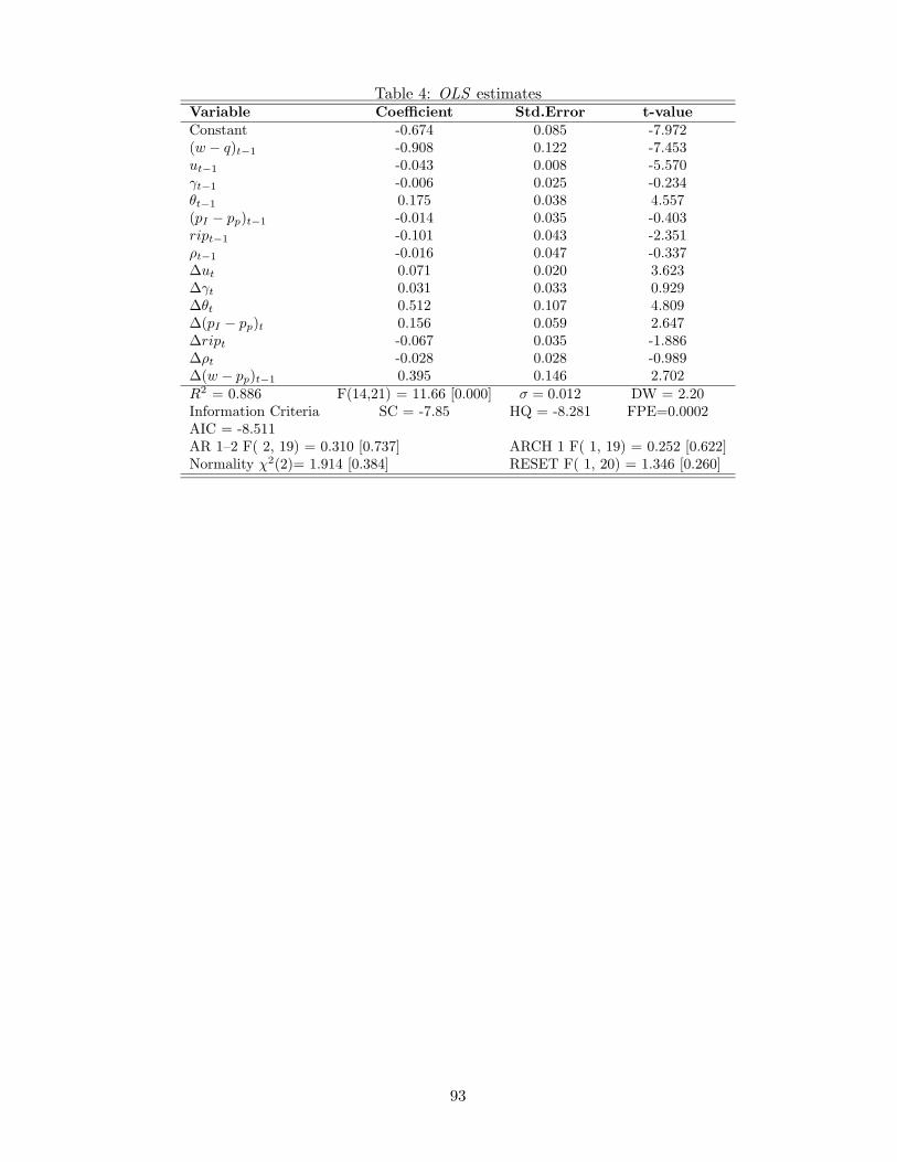
Table 4: OLS estimatesVariable Coefficient Std.Error t-value

Constant -0.674 0.085 -7.972(w − q)t−1 -0.908 0.122 -7.453ut−1 -0.043 0.008 -5.570γt−1 -0.006 0.025 -0.234θt−1 0.175 0.038 4.557(pI − pp)t−1 -0.014 0.035 -0.403ript−1 -0.101 0.043 -2.351ρt−1 -0.016 0.047 -0.337∆ut 0.071 0.020 3.623∆γt 0.031 0.033 0.929∆θt 0.512 0.107 4.809∆(pI − pp)t 0.156 0.059 2.647∆ript -0.067 0.035 -1.886∆ρt -0.028 0.028 -0.989∆(w − pp)t−1 0.395 0.146 2.702R2 = 0.886 F(14,21) = 11.66 [0.000] σ = 0.012 DW = 2.20Information Criteria SC = -7.85 HQ = -8.281 FPE=0.0002AIC = -8.511AR 1–2 F( 2, 19) = 0.310 [0.737] ARCH 1 F( 1, 19) = 0.252 [0.622]Normality χ2(2)= 1.914 [0.384] RESET F( 1, 20) = 1.346 [0.260]

93

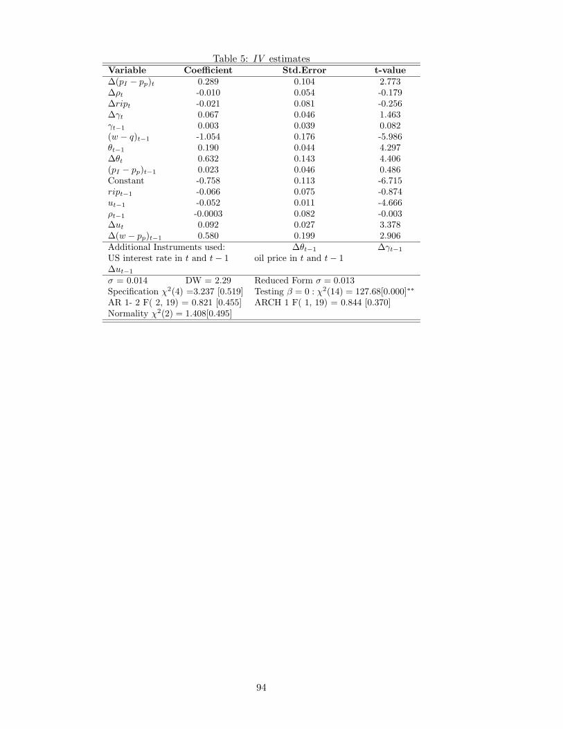
Table 5: IV estimatesVariable Coefficient Std.Error t-value

∆(pI − pp)t 0.289 0.104 2.773∆ρt -0.010 0.054 -0.179∆ript -0.021 0.081 -0.256∆γt 0.067 0.046 1.463γt−1 0.003 0.039 0.082(w − q)t−1 -1.054 0.176 -5.986θt−1 0.190 0.044 4.297∆θt 0.632 0.143 4.406(pI − pp)t−1 0.023 0.046 0.486Constant -0.758 0.113 -6.715ript−1 -0.066 0.075 -0.874ut−1 -0.052 0.011 -4.666ρt−1 -0.0003 0.082 -0.003∆ut 0.092 0.027 3.378∆(w − pp)t−1 0.580 0.199 2.906Additional Instruments used: ∆θt−1 ∆γt−1

US interest rate in t and t − 1 oil price in t and t − 1∆ut−1

σ = 0.014 DW = 2.29 Reduced Form σ = 0.013Specification χ2(4) =3.237 [0.519] Testing β = 0 : χ2(14) = 127.68[0.000]∗∗

AR 1- 2 F( 2, 19) = 0.821 [0.455] ARCH 1 F( 1, 19) = 0.844 [0.370]Normality χ2(2) = 1.408[0.495]

94

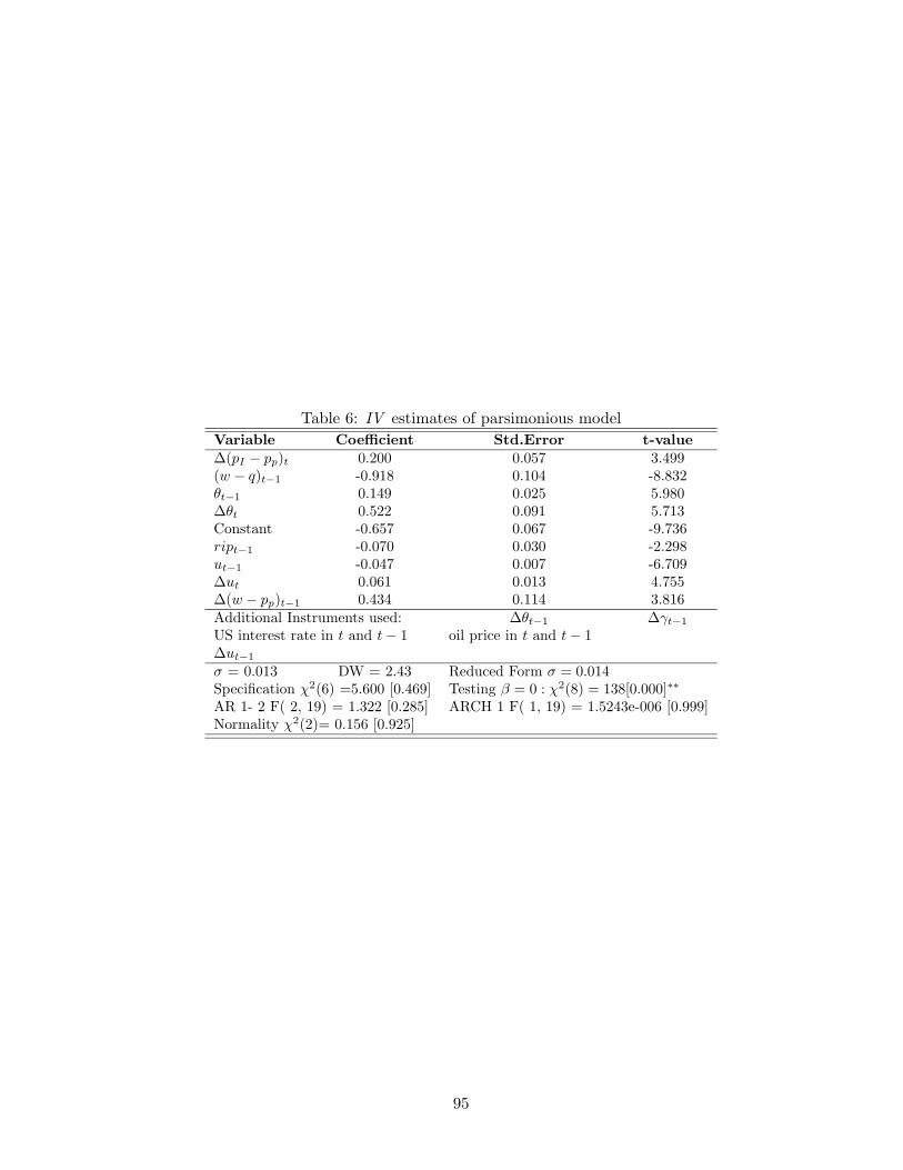
Table 6: IV estimates of parsimonious model

Variable Coefficient Std.Error t-value

∆(pI − pp)t 0.200 0.057 3.499(w − q)t−1 -0.918 0.104 -8.832θt−1 0.149 0.025 5.980∆θt 0.522 0.091 5.713Constant -0.657 0.067 -9.736ript−1 -0.070 0.030 -2.298ut−1 -0.047 0.007 -6.709∆ut 0.061 0.013 4.755∆(w − pp)t−1 0.434 0.114 3.816Additional Instruments used: ∆θt−1 ∆γt−1

US interest rate in t and t − 1 oil price in t and t − 1∆ut−1

σ = 0.013 DW = 2.43 Reduced Form σ = 0.014Specification χ2(6) =5.600 [0.469] Testing β = 0 : χ2(8) = 138[0.000]∗∗

AR 1- 2 F( 2, 19) = 1.322 [0.285] ARCH 1 F( 1, 19) = 1.5243e-006 [0.999]Normality χ2(2)= 0.156 [0.925]

95

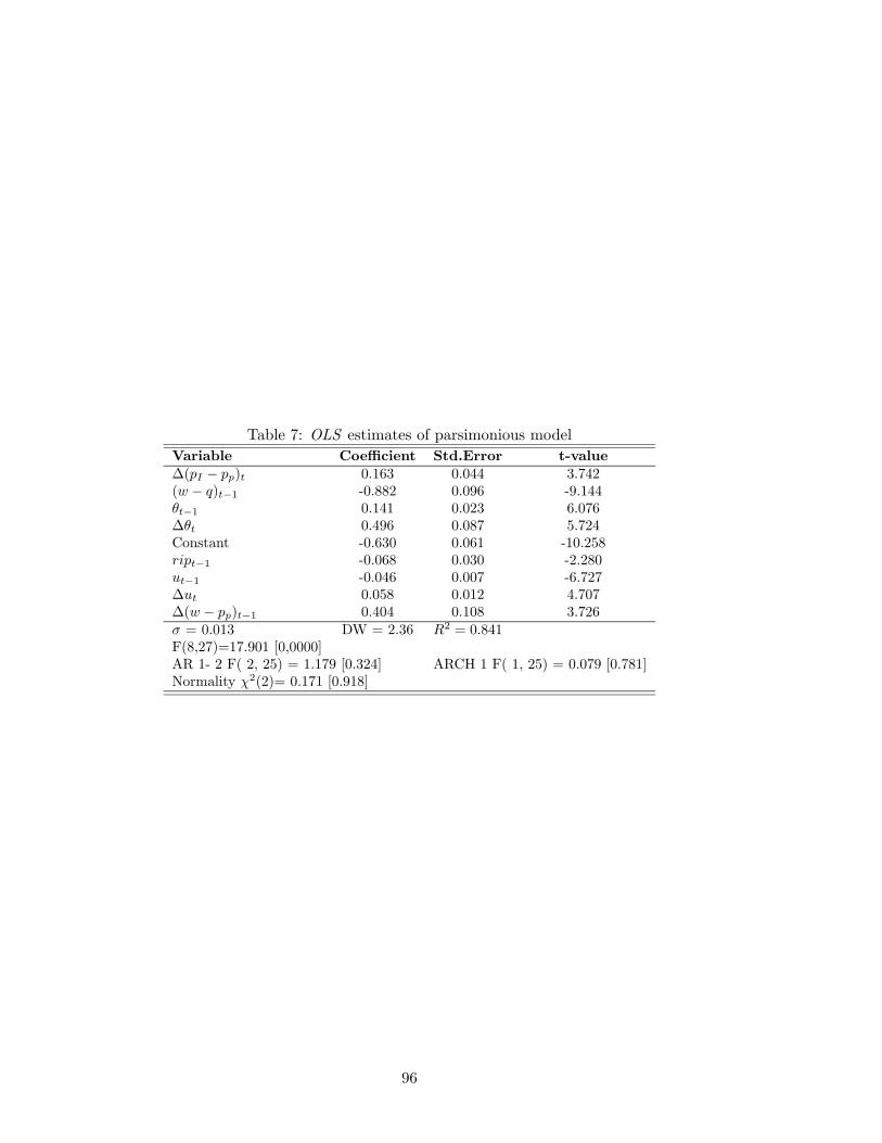
Table 7: OLS estimates of parsimonious model

Variable Coefficient Std.Error t-value

∆(pI − pp)t 0.163 0.044 3.742(w − q)t−1 -0.882 0.096 -9.144θt−1 0.141 0.023 6.076∆θt 0.496 0.087 5.724Constant -0.630 0.061 -10.258ript−1 -0.068 0.030 -2.280ut−1 -0.046 0.007 -6.727∆ut 0.058 0.012 4.707∆(w − pp)t−1 0.404 0.108 3.726σ = 0.013 DW = 2.36 R2 = 0.841F(8,27)=17.901 [0,0000]AR 1- 2 F( 2, 25) = 1.179 [0.324] ARCH 1 F( 1, 25) = 0.079 [0.781]Normality χ2(2)= 0.171 [0.918]

96

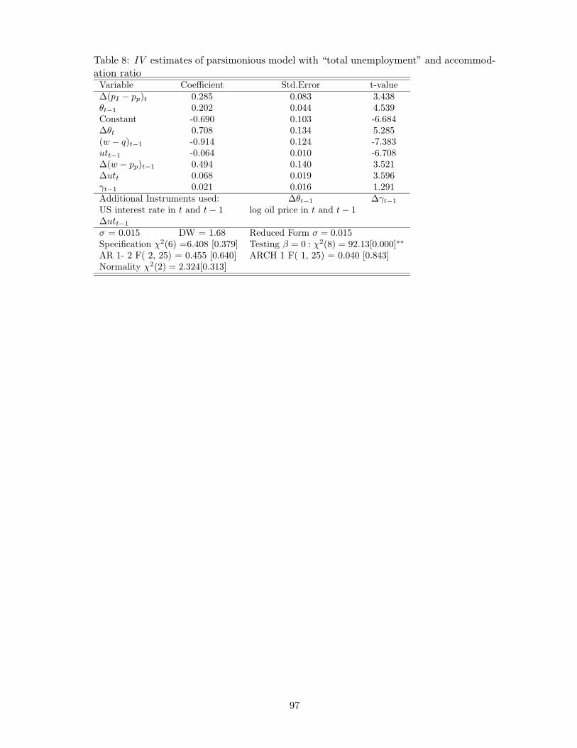
Table 8: IV estimates of parsimonious model with “total unemployment” and accommod-ation ratioVariable Coefficient Std.Error t-value∆(pI − pp)t 0.285 0.083 3.438θt−1 0.202 0.044 4.539Constant -0.690 0.103 -6.684∆θt 0.708 0.134 5.285(w − q)t−1 -0.914 0.124 -7.383utt−1 -0.064 0.010 -6.708∆(w − pp)t−1 0.494 0.140 3.521∆utt 0.068 0.019 3.596γt−1 0.021 0.016 1.291Additional Instruments used: ∆θt−1 ∆γt−1

US interest rate in t and t − 1 log oil price in t and t − 1∆utt−1



97

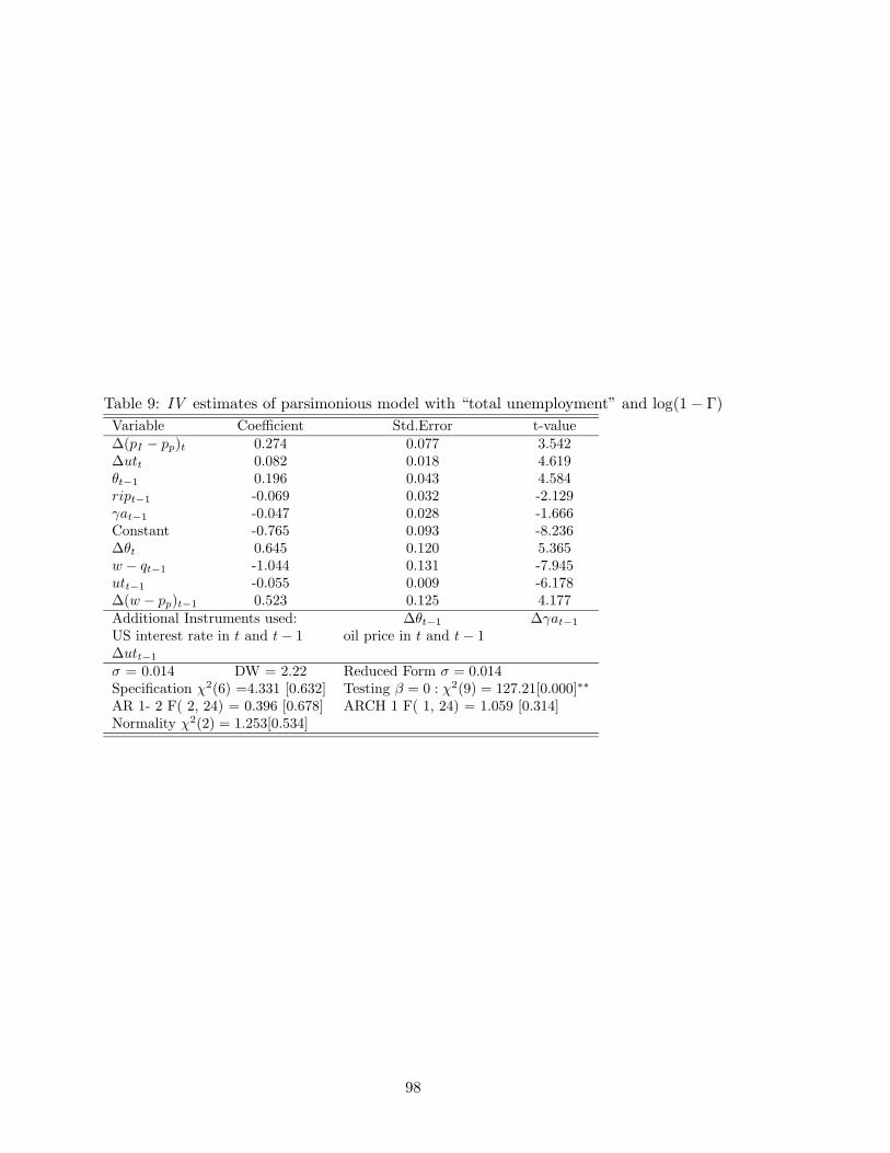
Table 9: IV estimates of parsimonious model with “total unemployment” and log(1 − Γ)

Variable Coefficient Std.Error t-value∆(pI − pp)t 0.274 0.077 3.542∆utt 0.082 0.018 4.619θt−1 0.196 0.043 4.584ript−1 -0.069 0.032 -2.129γat−1 -0.047 0.028 -1.666Constant -0.765 0.093 -8.236∆θt 0.645 0.120 5.365w − qt−1 -1.044 0.131 -7.945utt−1 -0.055 0.009 -6.178∆(w − pp)t−1 0.523 0.125 4.177Additional Instruments used: ∆θt−1 ∆γat−1

US interest rate in t and t − 1 oil price in t and t − 1∆utt−1



98

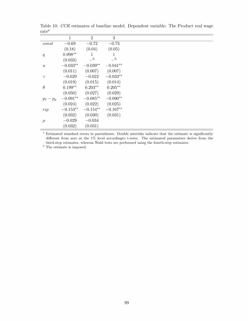
Table 10: CCR estimates of baseline model. Dependent variable: The Product real wageratea

1 2 3

const −0.69 −0.72 −0.73(0.18) (0.04) (0.05)

q 0.998∗∗ 1 1(0.033) −b −b

u −0.033∗∗ −0.039∗∗ −0.041∗∗

(0.011) (0.007) (0.007)γ −0.029 −0.022 −0.033∗∗

(0.019) (0.015) (0.014)θ 0.199∗∗ 0.203∗∗ 0.205∗∗

(0.050) (0.027) (0.029)pI − pp −0.091∗∗ −0.085∗∗ −0.090∗∗

(0.024) (0.022) (0.025)rip −0.153∗∗ −0.154∗∗ −0.167∗∗

(0.032) (0.030) (0.031)ρ −0.029 −0.034

(0.032) (0.031)

a Estimated standard errors in parentheses. Double asterisks indicate that the estimate is significantlydifferent from zero at the 1% level accordingto t-tests. The estimated parameters derive from thethird-step estimates, whereas Wald tests are performed using the fourth-step estimates.

b The estimate is imposed.

99

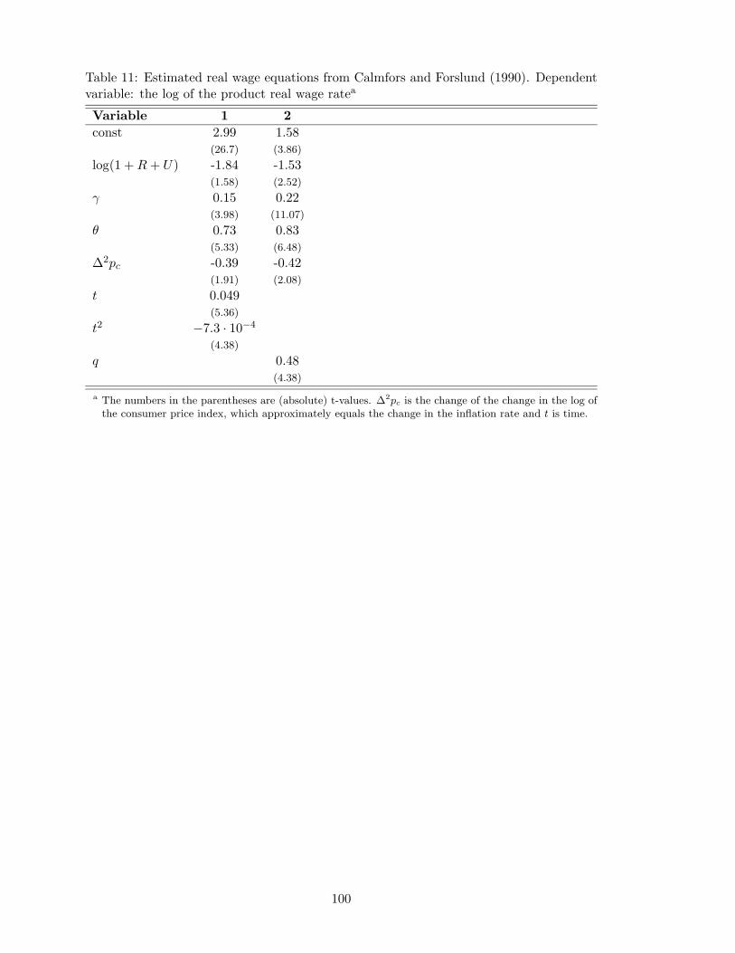
Table 11: Estimated real wage equations from Calmfors and Forslund (1990). Dependentvariable: the log of the product real wage ratea

Variable 1 2

const 2.99 1.58(26.7) (3.86)

log(1 + R + U) -1.84 -1.53(1.58) (2.52)

γ 0.15 0.22(3.98) (11.07)

θ 0.73 0.83(5.33) (6.48)

∆2pc -0.39 -0.42(1.91) (2.08)

t 0.049(5.36)

t2 −7.3 · 10−4

(4.38)

q 0.48(4.38)

a The numbers in the parentheses are (absolute) t-values. ∆2pc is the change of the change in the log ofthe consumer price index, which approximately equals the change in the inflation rate and t is time.

100

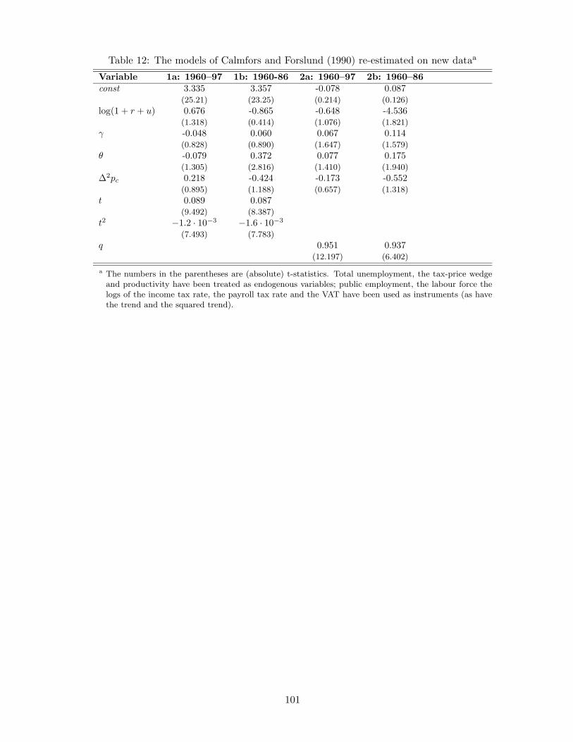
Table 12: The models of Calmfors and Forslund (1990) re-estimated on new dataa

Variable 1a: 1960–97 1b: 1960-86 2a: 1960–97 2b: 1960–86

const 3.335 3.357 -0.078 0.087(25.21) (23.25) (0.214) (0.126)

log(1 + r + u) 0.676 -0.865 -0.648 -4.536(1.318) (0.414) (1.076) (1.821)

γ -0.048 0.060 0.067 0.114(0.828) (0.890) (1.647) (1.579)

θ -0.079 0.372 0.077 0.175(1.305) (2.816) (1.410) (1.940)

∆2pc 0.218 -0.424 -0.173 -0.552(0.895) (1.188) (0.657) (1.318)

t 0.089 0.087(9.492) (8.387)

t2 −1.2 · 10−3 −1.6 · 10−3

(7.493) (7.783)

q 0.951 0.937(12.197) (6.402)

a The numbers in the parentheses are (absolute) t-statistics. Total unemployment, the tax-price wedgeand productivity have been treated as endogenous variables; public employment, the labour force thelogs of the income tax rate, the payroll tax rate and the VAT have been used as instruments (as havethe trend and the squared trend).

101

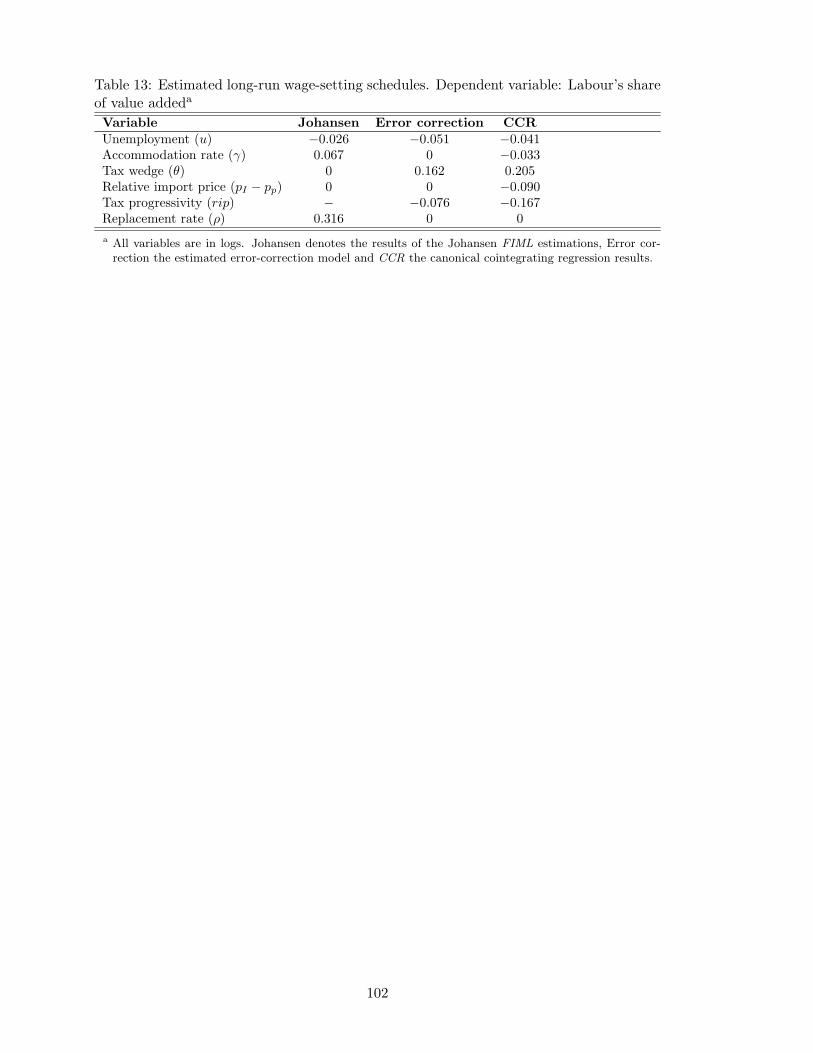
Table 13: Estimated long-run wage-setting schedules. Dependent variable: Labour’s shareof value addeda

Variable Johansen Error correction CCR

Unemployment (u) −0.026 −0.051 −0.041Accommodation rate (γ) 0.067 0 −0.033Tax wedge (θ) 0 0.162 0.205Relative import price (pI − pp) 0 0 −0.090Tax progressivity (rip) − −0.076 −0.167Replacement rate (ρ) 0.316 0 0

a All variables are in logs. Johansen denotes the results of the Johansen FIML estimations, Error cor-rection the estimated error-correction model and CCR the canonical cointegrating regression results.

102

ACTIVE LABOUR MARKET POLICIES AND REAL-WAGE DETERMINATION .../menu/standard/file/... · Running...

Documents

Transcript of ACTIVE LABOUR MARKET POLICIES AND REAL-WAGE DETERMINATION .../menu/standard/file/... · Running...