CCA30-

Comparative MolecularField Analysis (CoMFA)

Hugo KubinyiBASF AG, D-67056 Ludwigshafen, Germany

1 Introduction2 CoMFA Methodology3 Series Design and Training and Test Set Selection4 Pharmacophore Hypotheses and Alignment5 Box, Grid Size, and 3D Field Calculations6 Derivation and Validation of 3D QSAR Models7 Some Practical Problems8 CoMFA Applications in Drug Design9 Conclusions

10 Notes11 Related Articles12 References

Abbreviations

3DD three-dimensional;C D molar concentration of adrug; CBGD corticosteroid binding globulin; CoMFAD com-parative molecular field analysis; CoMSIAD comparative mo-lecular similarity indices analysis; GOLPED generating opti-mal linear PLS estimations; PLSD partial least squares;PRESSD predictive residual sum of squares; RMSD rootmean squares; TBGD testosterone binding globulin.

1 INTRODUCTION

Most drugs that are nowadays used in human therapy inter-act with certain macromolecular biological targets, e.g., withenzymes, receptors, ion channels, and transporters, in somecases even with desoxyribonucleic acid.1 3 With the exceptionof some irreversibly reacting enzyme inhibitors (e.g., acetylsal-icylic acid and penicillin) and of alkylating agents, most drugactions result from the noncovalent association of a small lig-and (the drug) to a specific binding site at the macromolecule.Thus, a precondition for the biological activity of a drug isits high affinity to this binding site. Enzyme inhibitors preventeither the binding of a substrate or the catalytic reaction at theactive site; receptor antagonists hinder the binding of an ago-nist or the adoption of an ‘active’ receptor conformation. Thesituation is more difficult with receptor agonists and partialagonists. In addition to their affinity to a certain binding site,they have different intrinsic activities, i.e., different abilities toproduce the agonist-mediated biological effect. Nowadays themost reasonable hypothesis is that receptor agonists stabilizethe ‘active’ conformation of a receptor, whereas antagonistsstabilize its ‘inactive’ conformation.1 4

The building blocks of all biological macromoleculesbelong to one group of optically active enantiomers. Thus, all

drug receptors (the term ‘receptor’ is most often generally usedfor any biological macromolecule which is the binding part-ner of a drug) are themselves enantiomers, i.e., they possessasymmetrical geometries. Therefore it is not surprising thatenantiomers of chiral drugs differ in their biological activities,a fact that is not adequately considered in most quantitativestructure activity relationships (QSAR) studies (cf. Sections 2and 4 andQSAR in Drug Design).

2 CoMFA METHODOLOGY

2.1 History

Classical QSAR correlates biological activities of drugswith physicochemical properties or indicator variables whichencode certain structural features.4 8 In addition to lipophilic-ity, polarizability, and electronic properties, steric parame-ters are also frequently used to describe the different sizeof substituents. In some cases, indicator variables have beenattributed to differentiate racemates and active enantiomers.5,6

However, in general, QSAR analyses consider neither the 3Dstructures of drugs nor their chirality.

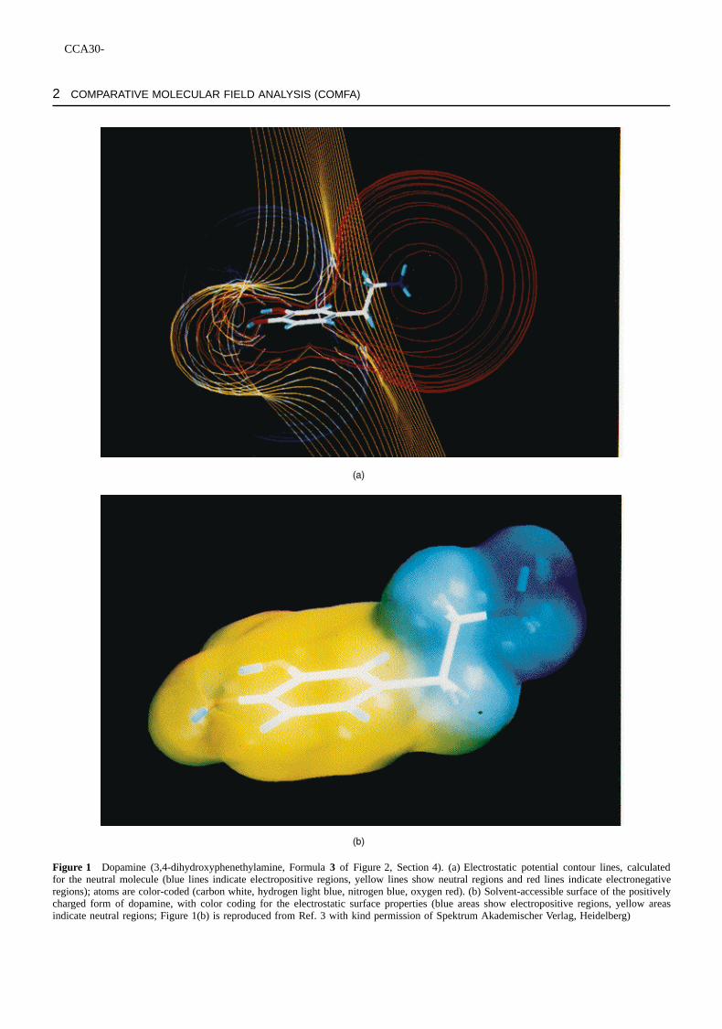
A binding site at a receptor which ‘looks’ at a ligandwould not see atoms and bonds, as we chemists do. Froma far distance, it would ‘feel’ the electrostatic potential of themolecule (Figure 1a) and, at a closer distance, the relativelyhard body of the molecule with its charge distribution patternat the solvent-accessible surface (Figure 1b).

In 1979, Cramer and Milne made a first attempt to comparemolecules by aligning them in space and by mapping theirmolecular fields to a 3D grid.9 In the following years, thisapproach was further developed as the DYLOMMS (dynamiclattice-oriented molecular modelling system) method10 but wasnot very well accepted by the scientific community. Severalimportant facts had to work together to allow a broaderapplication of this approach:

1. In 1986, Svante Wold proposed the use of partial leastsquares (PLS) analysis, instead of principal componentanalysis, to correlate the field values with the biologicalactivities (seePartial Least Squares (PLS) in Chemistry);

2. in 1988, a key publication appeared in theJournal of theAmerican Chemical Society11 and the method was calledcomparative molecular field analysis (CoMFA) from thenon; and

3. appropriate software became commercially available.12

Since 1988, a few hundred publications, several reviews(e.g., Refs. 1318), and three books10,19 have appeared on thissubject. Despite some major problems in its proper application(cf. Section 7), the method is now generally estimated as auseful tool for deriving 3D QSAR models.

2.2 Steps of a CoMFA

CoMFAs describe 3D structureactivity relationships in aquantitative manner. For this purpose, a set of molecules isfirst selected which will be included in the analysis. As amost important precondition, all molecules have to interactwith the same kind of receptor (or enzyme, ion channel,transporter) in the same manner, i.e., with identical binding

CCA30-

2 COMPARATIVE MOLECULAR FIELD ANALYSIS (COMFA)

Figure 1 Dopamine (3,4-dihydroxyphenethylamine, Formula3 of Figure 2, Section 4). (a) Electrostatic potential contour lines, calculatedfor the neutral molecule (blue lines indicate electropositive regions, yellow lines show neutral regions and red lines indicate electronegativeregions); atoms are color-coded (carbon white, hydrogen light blue, nitrogen blue, oxygen red). (b) Solvent-accessible surface of the positivelycharged form of dopamine, with color coding for the electrostatic surface properties (blue areas show electropositive regions, yellow areasindicate neutral regions; Figure 1(b) is reproduced from Ref. 3 with kind permission of Spektrum Akademischer Verlag, Heidelberg)

CCA30-

COMPARATIVE MOLECULAR FIELD ANALYSIS (COMFA) 3

sites in the same relative geometry. In the next step, a certainsubgroup of molecules is selected which constitutes a trainingset to derive the CoMFA model. The residual molecules areconsidered to be a test set which independently proves thevalidity of the derived model(s) (Section 3). Atomic partialcharges are calculated and (several) low energy conformationsare generated. A pharmacophore hypothesis is derived to orientthe superposition of all individual molecules and to afford arational and consistent alignment (Section 4).

A sufficiently large box is positioned around the moleculesand a grid distance is defined. Different atomic probes, e.g., acarbon atom, a positively or negatively charged atom, a hydro-gen bond donor or acceptor, or a lipophilic probe, are used tocalculate field values in each grid point, i.e., the energy val-ues which the probe would experience in the correpondingposition of the regular 3D lattice (Section 5). These ‘fields’correspond to tables, most often including several thousandsof columns, which must be correlated with the binding affini-ties or with other biological activity values. PLS analysis isthe most appropriate method for this purpose (Section 6). Nor-mally cross-validation is used to check the internal predictivityof the derived model.

The result of the analysis corresponds to a regression equa-tion with thousands of coefficients. Most often it is presentedas a set of contour maps. These contour maps show favor-able and unfavorable steric regions around the molecules aswell as favorable and unfavorable regions for electropositiveor electronegative substituents in certain positions (Section 6).Predictions for the test set (the compounds not included in theanalysis) and for other compounds can be made, either by aqualitative inspection of these contour maps or, in a quantita-tive manner, by calculating the fields of these molecules andby inserting the grid values into the PLS model (Section 6).

Despite the straightforward definition of CoMFA, there area number of serious problems and possible pitfalls.10 Sev-eral CoMFA modifications have been described which solve oravoid some of these problems (Section 7).19 In addition, alter-natives to CoMFA were developed, e.g., comparative molec-ular similarity indices analysis (CoMSIA) (Section 5)19,20 andother 3D quantitative similarityactivity relationship (QSiAR)methods.21 24

2.3 A CoMFA Application

The first application of CoMFA11 is an illustrative example.It correlates the binding affinities of 21 steroids (e.g.,1 and2) to human corticosteroid (CBG) and testosterone bindingglobulins (TBG). Since steroids are relatively rigid systems(with the exception of the side chains in position 17), thealignment was performed by a rigid body RMS fit of carbonatoms 3, 5, 6, 13, 14, and 17.

1 2

3 56

1314

17

R1

O

R2

H

R1R2

H

OH

The results, using different options, indicated that the stericfield mostly led to an explanation of the variance in the

binding data. The fit of the affinity values, expressed by thesquared correlation coefficientr2, was close to 0.9 (0.897 forCBG and 0.873 for TBG). After cross-validation (Section 6),a predictive squared correlation coefficientQ2 of around 0.6(0.662 for CBG and 0.555 for TBG) was obtained. Mostinteresting is the result of the prediction for ten compounds notincluded in the original CoMFA studies. For the CBG bindingdata of compounds #2231 (for structures and numberingsee Ref. 11), anr2

predD 0.65 was given. However, this valuemust be wrong, owing to a misplacement of compound #7in Figure 7 of Ref. 11; the correct value isr2

predD 0.31.20,24

A possible explanation for this poor test set predictivity isdiscussed in Section 3.

3 SERIES DESIGN AND TRAINING AND TEST SETSELECTION

The application of statistical methods depends on a properexperimental design, for the training set from which a QSARmodel is derived, as well as for the test set, for which biologicaldata shall be predicted (e.g., Refs. 4, 5, 10). In QSAR analyses,this important precondition is most often neglected. No wonderthat in such cases problems arise from a biased object selectionand from different structural and parameter spaces of thetraining and test sets.

The training set compounds should span a parameter spacein which all data points are more or less equally distributed.The structures and all relevant properties of the test set com-pounds should not be too far from the test set compounds. Toderive statistical models with reasonable experimental effort,an appropriate design scheme should be used to cover theproperty space with the smallest possible number of objects.Redundancy is minimized by following this recommenda-tion. On the other hand, some redundancy should be includedto avoid the possibility that cross-validation (Section 6) isno longer applicable and that single point errors distort thefinal QSAR model. Especially the latter topic is most oftenneglected as a possible reason for poor test set prediction.Reasonable results for the test set predictions can only beexpected by including sufficient redundancy in the trainingset compounds.

Most QSAR and 3D QSAR studies are retrospective anal-yses without an appropriate series design. The consequencesare either a poor fit of the training set data or a lack of predic-tivity for the test set compounds. The poor predictivity of theCBG CoMFA models (compounds1 and2; Section 2.3) is notsurprising if one considers that compound #23 is the only onein the whole data set which bears a 21-acetoxy group and thatalso compound #31, a 9-fluoro-substituted steroid, is outsidethe structural space of the training set.

The problems of this data set are easily understood if aFree Wilson analysis is applied.4 6 The training set com-pounds (#121) can be described by a simple one-parameterregression equation (equation 1; the term 4,5CDC indicatesthe presence or absence of a cycloaliphatic 4,5-double bondin ring A of the steroids).24 The internal predictivity of thismodel (Q2 D 0.726;sPRESSD 0.630) and the test set predictiv-ity (n D 10; r2

predD 0.477; sPRESSD 0.733) are even slightlybetter than the CoMFA result (Section 2.3).

log 1/CBGD 2.022.š0.52/4,5 CDC C 5.186.š0.36/

CCA30-

4 COMPARATIVE MOLECULAR FIELD ANALYSIS (COMFA)

.n D 21;r D 0.882;s D 0.568;F D 66.41;

Q2 D 0.726;sPRESSD 0.630/ .1/

Selection of compounds #112 and #2331 (instead ofcompounds #121) gives a much better presentation of thestructural space in the training set and, correspondingly, asignificantly better prediction of the binding affinities of thetest set compounds (see below). Equation (2) is obtained ifcompounds #112 and #2331 are used as the training set(n D 21).24

log 1/CBGD 1.667.š0.75/4,5 CDC C 5.306.š0.65/

.n D 21;r D 0.731;s D 0.697;F D 21.82;

Q2 D 0.454;sPRESSD 0.754/ .2/

Despite the worse fit and internal predictivity, as com-pared with equation (1), the validity of this model is provenby its excellent test set (compounds #1322) predictivity:r2predD 0.909; sPRESSD 0.406). The differences between both

models, especially in their test set predictivity, provide strikingevidence for the influence of the training and test set selectionson the obtained results. Thus, a careful selection of the train-ing set molecules is of utmost importance. A broad variety ofstructural features should be included in these molecules, inorder to allow reliable predictions for the test set compounds.

4 PHARMACOPHORE HYPOTHESES ANDALIGNMENT

The specific interaction of drugs with proteins dependson a structural complementarity between the ligand and itsbinding site, in the 3D arrangement of all relevant molecularproperties. Pharmacophores are 3D models of such structuralfeatures (Figure 2), in the simplest case a 2D three-pointpharmacophore.

The strategy applied in Figure 2 is called the ‘active analogapproach’4,5,10; flexible compounds are compared with rigidanalogs, in order to determine which geometry of a flexibleligand corresponds to the biologically active conformation.Any rigidization of a flexible drug in a wrong geometry leadsto inactive molecules. On the other hand, experience showsthat freezing the bioactive conformation of a ligand may leadto superactive and highly selective analogs.1 3

As already mentioned (Section 1), enantiomers of chiralcompounds differ in their biological effects. This can be easilyillustrated by the different odors of the closely related monoter-penes (R)- and (S)-limonene and (R)- and (S)-carvone (9a,band 10a,b; Figure 3), which result from the stereospecificinteraction of these compounds with the olfactory G-protein-coupled receptors.

With respect to their relative affinities to a chiral bindingsite, all different pairs of enantiomers differ more or less intheir relative affinities. Eudismic ratios, i.e., the ratio of theaffinity or biological activity of the ‘more’ active analog (theeutomer) to the ‘less’ active one (the distomer) between 1 and500 000 have been observed (e.g., Refs. 3, 25, 26).

Whereas the alignment of compounds1 and2 (Section 2.3)seems to be obvious, there are more complex situations whichdemand a detailed analysis of the functional group similarityof the compounds in different orientations, as is e.g., the casefor dihydrofolate11 and methotrexate12 (Figure 4).3,5,10,27

Figure 2 Dopamine 3 is a neurotransmitter with two phenolichydroxy groups, a phenyl ring and a positively charged ammoniumgroup, separated from the aromatic ring by two carbon atoms. Cor-respondingly, a pharmacophore model can be defined which containstwo donor/accptor groups D/A, a positively charged donor group PD,and a lipophilic area L (model below structure3). However, dopaminehas two flexible bonds. Rotation around the angles�1 or �2 leadsto other geometries, with different distancesd1 and d2. To differ-entiate between the rotamers, i.e., between different conformations,compounds4 and 5 (racemic mixtures) have been investigated. Invivo, compound4 is the more active analog. If both compounds are,however, directly injected into dopamine-receptive brain areas of therat, the 5,6-dihydroxy analog5 is 100 times more active, according tothe dopamine conformation presented in6. Accordingly, apomorphine7 and some analogs and derivatives of lysergic acid8 are dopamineagonists. Under the assumption of similar binding modes, the phar-macophore geometries shown in red allow a mutual alignment ofcompounds5 8

CH3 CH3 CH3

O

CH3

O

(R)-(+)- (S)-(-)- (S)-(+)- (R)-(-)-

limonene carvone

orange lemon caraway spearmint

9a 9b 10a 10b

Figure 3 Enantiomers of chiral drugs show different biologicalproperties. The monoterpenes (R)- and (S)-limonene (9a, b) and(R)- and (S)-carvone (10a, b) interact with the olfactory receptors(which are, like many drug receptors, G-protein-coupled receptors) ina different manner, producing different odors that are indicated underthe individual formulas

A common pharmacophore within a series of compoundsdoes not necessarily mean that all compounds need to haveidentical molecular frames. One of the most important advan-tages of the CoMFA method results from the fact that mole-cules with identical pharmacophores but different atom con-nectivities can be combined in one analysis.

The superposition of all molecules is performed accordingto the equivalent functional groups that are identified as thepharmacophore, either by hand or by an appropriate fieldfit.10,28 A valuable tool for the superposition of moleculeswithin a congeneric series of compounds is the programSEAL.29 It allows the definition of a ‘similarity index’AF(equation 3) between two molecules A and B in any relativeorientation to each other. For this purpose, atomic similarity

CCA30-

COMPARATIVE MOLECULAR FIELD ANALYSIS (COMFA) 5

N

N N

N

N

N

R

N

N N

N

OH

N

H

R

N

N O

N

N

N

R

+

11

12

11

H

H H

H

H

H H

H H

H

H

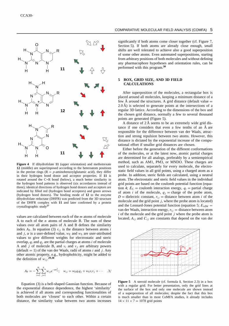
Figure 4 If dihydrofolate 11 (upper orientation) and methotrexate12 (middle) are superimposed according to the heteroatom positionsin the pterine rings (RD p-aminobenzoylglutamic acid), they differin their hydrogen bond donor and acceptor properties. If11 isrotated around the CR bond (below), a much better similarity inthe hydrogen bond patterns is observed (six accordances instead ofthree); identical directions of hydrogen bond donors and acceptors areindicated by filled red (hydrogen bond acceptors) and green arrows(hydrogen bond donors). The binding mode of12 to the enzymedihydrofolate reductase (DHFR) was predicted from the 3D structureof the DHFR complex with11 and later confirmed by a proteincrystallographic study27

values are calculated between each of them atoms of moleculeA to each of then atoms of molecule B. The sum of thesevalues over all atom pairs of A and B defines the similarityindex AF. In equation (3)rij is the distance between atomsiandj, ˛ is a user-defined value,wE andwS are user-attributedvalues to give different weights for electrostatic and stericoverlap,qi andqj are the partial charges at atomsi of moleculeA and j of molecule B, andvi and vj are arbitrary powers(defaultD 1) of the van der Waals, radii of atomsi andj. Anyother atomic property, e.g., hydrophobicity, might be added tothe definition ofwij.29,30

AF D �m∑iD1

n∑jD1

wije�˛r2ij ; wij D wEqiqj C wSvivj C Ð Ð Ð .3/

Equation (3) is a bell-shaped Gaussian function. Because ofthe exponential distance dependence, the highest ‘similarity’is achieved if all atoms and corresponding functionalities ofboth molecules are ‘closest’ to each other. Within a certaindistance, the similarity value between two atoms increases

significantly if both atoms come closer together (cf. Figure 7,Section 5). If both atoms are already close enough, smallshifts are well tolerated to achieve also a good superpositionof some other atoms. Even automated superpositions, startingfrom arbitrary positions of both molecules and without definingany pharmacophore hypotheses and orientation rules, can beperformed with this program.30

5 BOX, GRID SIZE, AND 3D FIELDCALCULATIONS

After superposition of the molecules, a rectangular box isplaced around all molecules, keeping a minimum distance of afew A around the structures. A grid distance (default valueD2.0A) is selected to generate points at the intersections of aregular 3D lattice. According to the dimensions of the box andthe chosen grid distance, normally a few to several thousandpoints are generated (Figure 5).

A distance of 2A seems to be an extremely wide grid dis-tance if one considers that even a few tenths of anA areresponsible for the difference between van der Waals, attrac-tion and strong repulsion between two atoms. However, thisdistance is dictated by the exponential increase of the compu-tational effort if smaller grid distances are chosen.

Either before the generation of the different conformationsof the molecules, or at the latest now, atomic partial chargesare determined for all analogs, preferably by a semiempiricalmethod, such as AM1, PM3, or MNDO. These charges areused to calculate, separately for every molecule, the electro-static field values in all grid points, using a charged atom as aprobe. In addition, steric fields are calculated, using a neutralatom. The electrostatic and steric field values in the individualgrid points are based on the coulomb potential function (equa-tion 4; EC D coulomb interaction energy,qi D partial chargeof atom i of the molecule,qj D charge of the probe atom,D D dielectric constant,rij D distance between atomi of themolecule and the grid pointj, where the probe atom is located)and the Lennard-Jones potential function (equation 5;EvdW Dvan der Waals, interaction energy,rij D distance between atomi of the molecule and the grid pointj where the probe atom islocated;Aij andCij are constants that depend on the van der

O

CH3CH3 R

Figure 5 A steroid molecule (cf. formula1, Section 2.3) in a boxwith a regular grid. For better presentation, only the grid lines atthe surface of the box and only one molecule are shown insteadof a superposition of all molecules; despite the fact that this boxis much smaller than in most CoMFA studies, it already includes14ð 11ð 7D 1078 grid points

CCA30-

6 COMPARATIVE MOLECULAR FIELD ANALYSIS (COMFA)

Waals, radii of the corresponding atoms), respectively.10,11

EC Dn∑iD1

qiqjDrij

.4/

EvdW Dn∑iD1

.Aijr�12ij �Cijr�6

ij / .5/

In close proximity to the surface of the atoms both poten-tials have very steep slopes. They approach infinite values ifthe atom positions of two molecules overlap. To avoid this,arbitrary cut-offs are defined and all larger positive (or nega-tive) values are set to these cut-off values (Figure 6).

In addition or alternatively to these fields, hydrophobicfields, calculated e.g., by the program HINT,10,31 or GRIDfields10,32 can be used. Arbitrary weights may be attributedto the different fields. An appropriate scaling of all vari-ables has to be performed if additional properties, e.g., thelipophilicity parameter logP (P D n-octanol/water partitioncoefficient),4 8,33 are included, to give a comparable weightto the individual fields and the single parameter(s).

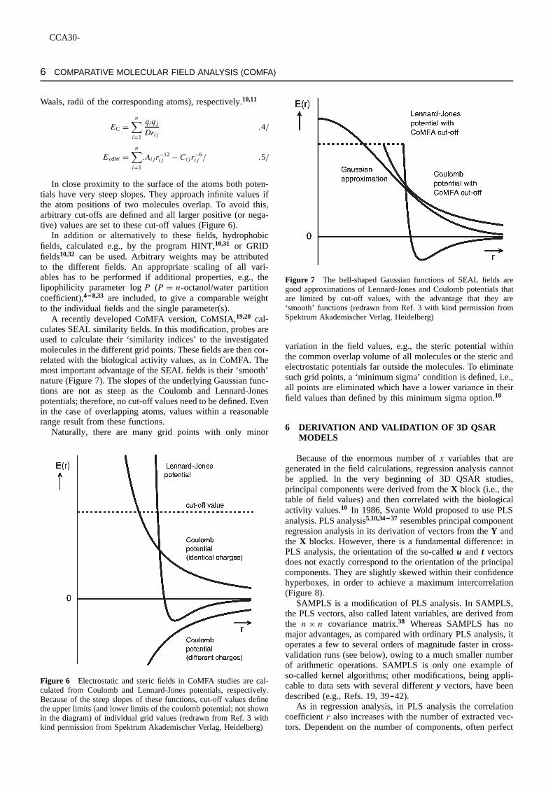
A recently developed CoMFA version, CoMSIA,19,20 cal-culates SEAL similarity fields. In this modification, probes areused to calculate their ‘similarity indices’ to the investigatedmolecules in the different grid points. These fields are then cor-related with the biological activity values, as in CoMFA. Themost important advantage of the SEAL fields is their ‘smooth’nature (Figure 7). The slopes of the underlying Gaussian func-tions are not as steep as the Coulomb and Lennard-Jonespotentials; therefore, no cut-off values need to be defined. Evenin the case of overlapping atoms, values within a reasonablerange result from these functions.

Naturally, there are many grid points with only minor

Figure 6 Electrostatic and steric fields in CoMFA studies are cal-culated from Coulomb and Lennard-Jones potentials, respectively.Because of the steep slopes of these functions, cut-off values definethe upper limits (and lower limits of the coulomb potential; not shownin the diagram) of individual grid values (redrawn from Ref. 3 withkind permission from Spektrum Akademischer Verlag, Heidelberg)

Figure 7 The bell-shaped Gaussian functions of SEAL fields aregood approximations of Lennard-Jones and Coulomb potentials thatare limited by cut-off values, with the advantage that they are‘smooth’ functions (redrawn from Ref. 3 with kind permission fromSpektrum Akademischer Verlag, Heidelberg)

variation in the field values, e.g., the steric potential withinthe common overlap volume of all molecules or the steric andelectrostatic potentials far outside the molecules. To eliminatesuch grid points, a ‘minimum sigma’ condition is defined, i.e.,all points are eliminated which have a lower variance in theirfield values than defined by this minimum sigma option.10

6 DERIVATION AND VALIDATION OF 3D QSARMODELS

Because of the enormous number ofx variables that aregenerated in the field calculations, regression analysis cannotbe applied. In the very beginning of 3D QSAR studies,principal components were derived from theX block (i.e., thetable of field values) and then correlated with the biologicalactivity values.10 In 1986, Svante Wold proposed to use PLSanalysis. PLS analysis5,10,34 37 resembles principal componentregression analysis in its derivation of vectors from theY andthe X blocks. However, there is a fundamental difference: inPLS analysis, the orientation of the so-calledu and t vectorsdoes not exactly correspond to the orientation of the principalcomponents. They are slightly skewed within their confidencehyperboxes, in order to achieve a maximum intercorrelation(Figure 8).

SAMPLS is a modification of PLS analysis. In SAMPLS,the PLS vectors, also called latent variables, are derived fromthe nð n covariance matrix.38 Whereas SAMPLS has nomajor advantages, as compared with ordinary PLS analysis, itoperates a few to several orders of magnitude faster in cross-validation runs (see below), owing to a much smaller numberof arithmetic operations. SAMPLS is only one example ofso-called kernel algorithms; other modifications, being appli-cable to data sets with several differenty vectors, have beendescribed (e.g., Refs. 19, 3942).

As in regression analysis, in PLS analysis the correlationcoefficientr also increases with the number of extracted vec-tors. Dependent on the number of components, often perfect

CCA30-

COMPARATIVE MOLECULAR FIELD ANALYSIS (COMFA) 7

BA1

BA2

BA3

::::

BAn

Y vector X matrix

u11

u12

u13

::::

u1n ....

PLSanalysis

c11 c21 c31 .... cn1

c21 c22 c32 .... cn2

c31 c32 c33 .... cn3

: : : :: : : :: : : :

cn1 cn2 cn3 . . . . cnn

t11

t12

t13

::::

t1n

t21

t22

t23

::::

t2n

, ,

covariance matrix

SAMPLSanalysis

From u = kt (k = constants k1, k2 ... kj;j = number of PLS components) follows:

BAi = a1Si1 + a2Si2 + a3Si3 + ... + amSim ++ b1Ei1 + b2Ei2 + b3Ei3 + ... + bmEim

S11

S21

S31

::::

Sn1

S12

S22

S32

::::

Sn2

S13

S23

S33

::::

S3n

S1m

S2m

S3m

::::

Snm

E11

E21

E31

::::

En1

E12 . . .. .E22 . . . . .E32 . . . . .

::::

En2 . . . . .

E1m

E2m

E3m

::::

Enm

S14 . . . . .S24 . . . . .S34 . . . . .

::::

Sn4 . . . . .

˚˚ ˚˚

˚˚˚

˚˚

X1

X2

X3

: : : :

Figure 8 PLS analysis derives vectorsu andt from theY block (ory vector; BAi D logarithms of relative affinities or other biologicalactivities) and theX block (Sij D steric field variable of moleculeiin the grid pointj; Eij D electrostatic field variable of moleculeiin the grid pointj) that are related to principal components. These‘latent variables’ are skewed within their confidence hyperboxes toachieve a maximum intercorrelation (diagram). SAMPLS is a PLSmodification which first derives the covariance matrix of theX blockand then the PLS result from this covariance matrix. Especially incross-validation (see below), SAMPLS analysis is much faster thanordinary PLS analysis

correlations are obtained in PLS analyses, owing to the largenumber ofx variables. Correspondingly, the goodness of fitis no criterion for the validity of a PLS model. The sig-nificance of additional PLS vectors is determined by cross-validation.10,35 37,43 In the most common leave-one-out cross-validation, one object (i.e., one biological activity value) iseliminated from the training set and a PLS model is derivedfrom the residual compounds. This model is used to pre-dict the biological activity value of the compound which wasnot included in the model. The same procedure is repeatedafter elimination of another object until all objects have been

eliminated once. The sum of the squared differences, PRESSD.ypred� yobs/2, between these ‘outside-predictions’ and theobservedy values is a measure for the internal predictivity ofthe PLS model. For larger data sets, an alternative to the leave-one-out technique is recommended to yield more stable PLSmodels. Several objects are eliminated from the data set at atime, randomly or in a systematic manner, and the excludedobjects are predicted by the corresponding model.10,43

In cross-validation, aQ2 (r2PRESS) value is defined like

r2 in regression and PLS analysis, using PRESS instead ofthe unexplained variance.ycalc� yobs/2. Cross-validatedQ2

values are always smaller than ther2 values, including allobjects (r2

FIT). As long as only significant PLS vectors arederived,Q2 increases, whereas decreasingQ2 values indicateoverprediction. In severe cases of overprediction PRESS maybecome even larger than the overall variance of they values;then negativeQ2 values are obtained, indicating that thepredictions from the model are worse than ‘no model’, i.e.,taking theymeanvalues as ‘predictions’.10,35,43The significanceof leave-one-out cross-validation results has to be commentedon: in highly redundant data sets, where all or at least mostobjects have close neighbors in multidimensional parameterspace, this procedure gives a much too optimistic result.

The standard deviation of predictions,sPRESS, is calculatedfrom PRESS, the sum of the squared errors of these predic-tions, considering the number of degrees of freedom. SDEP(the standard deviation of the error of predictions)10 corre-sponds tosPRESSbut the number of degrees of freedom is notconsidered in the calculation of the SDEP value. The smallestsPRESSor SDEP value should be taken as the criterion for theoptimum number of components. Alternatively, an increase oftheQ2 value by a certain percentage, e.g., 5%, may be definedas the criterion to accept a further PLS component. As long asonly significant components are extracted in the PLS analysis,PRESS, SDEP andsPRESSwill decrease; if too many compo-nents are derived, overprediction results and PRESS, SDEPandsPRESSincrease.

Bootstrapping is a procedure in whichn random selectionsout of the original set ofn objects are performed several timesto simulate different samplings from a larger set of objects.In each run some objects may not be included in the PLSanalysis, whereas some others might be included more thanonce. Confidence intervals for each term can be estimatedfrom such a procedure, giving an independent measure of thestability of the PLS model.10,36,43

A rigorous alternative to cross-validation and bootstrappingdemands a repetitive scrambling of they values. Only ifthe results from a PLS model, using the original order ofthe y values, is significantly better than the results from the‘scrambled’ models, using randomly orderedy values in thePLS analysis, can one be sure that a relationship indeed existsbetween the biological data and theX block.

Although the PLS method is claimed to be a robust mod-eling technique, experience shows that too many noise vari-ables, i.e., variables that do not contribute to prediction,obscure the result. For prediction such additional variablesare most often useless or even detrimental. The problemof perturbation of CoMFA models by many irrelevant gridpoints has been approached by developing a variable selec-tion procedure, called GOLPE (generating optimal linear PLSestimations).10,36,37In GOLPE, first a D-optimal design is used

CCA30-

8 COMPARATIVE MOLECULAR FIELD ANALYSIS (COMFA)

Figure 9 3D contour maps around testosterone (1, Section 2.3; R1 D OH, R2 D H) as the result of a CoMFA analysis of the TBG affinities ofdifferent steroids.11 (a) The color codings indicate regions where electronegative substituents enhance (blue) or reduce (red) the binding affinity.(b) Regions where substitution enhances (green) or reduces (yellow) the binding affinity (reproduced from Ref. 13 with kind permission fromVCH, Weinheim)

CCA30-

COMPARATIVE MOLECULAR FIELD ANALYSIS (COMFA) 9

to preselect nonredundant variables. A subset of variables,having a higher degree of orthogonality in multidimensionalparameter space, is selected by this procedure. Then a frac-tional factorial design is used to run PLS analyses with differ-ent combinations of these variables. The predictive abilities ofthe models are checked by a cross-validation procedure. Theinfluence of every variable can be estimated from a compari-son of the PRESS values of the models including this variableand those not containing it. Explanatory variables, i.e., gridpoints that significantly contribute to prediction, are kept, allothers are eliminated.

The results of a PLS analysis can be transformed to regres-sion coefficients of theX block variables that are used forthe calculation and prediction of biological activity values.Because of the large number of regression coefficients, a directinterpretation of the corresponding equation is impossible. Anappropriate way to visualize the results is the generation ofcontour maps which show the volumes of regions that arelarger or smaller than certain user-defined positive or negativevalues (Figures 9a and 9b).

7 SOME PRACTICAL PROBLEMS

Because of the complexity of the CoMFA method, manydifferent problems arise in running the analyses and in inter-preting the results obtained (see e.g., Refs. 10, 11, 1519).

The search for the ‘bioactive’ conformation and the com-mon pharmacophore constitutes a serious problem. It is oneof the most important sources of wrong conclusions anderrors in all CoMFA studies. The risk of deriving irrelevantgeometries can only be reduced by a consideration of rigidanalogs. Even then, the alignment poses problems becausethere are many cases of different binding modes of seem-ingly closely related analogs. The more X-ray structures ofligand protein complexes are determined, the larger becomesthe number of examples where such unexpected binding modesare observed.3,5,10,44

Another possible source of error is the mutual alignmentof all molecules. Because the training set contains active andinactive molecules, too much weight might be attributed to the3D structures of the inactive compounds in the mutual align-ment. CoMFA models have been refined by a re-alignmentof the training set molecules, guided by the first, preliminaryCoMFA results; molecules for which too low activities arecalculated, are reoriented to achieve an ‘improved’ (but moresubjective) alignment.45 The definition of pairwise similarityindices of molecules, derived from 3D fields, would allowpairwise alignments, without any consideration of all othermolecules;24 the disadvantage of this approach is the loss ofthe 3D information for predictions.

Of course, any risks in the generation of the conformationsand in the alignment could be avoided by looking at the 3Dstructures of ligandprotein complexes which are derived fromX-ray crystallographic or multidimensional NMR studies.46,47

The advantage of such a procedure is obvious but the questionarises: is CoMFA really the adequate tool for such cases?

The problems of inadequate training and test set selectionshave already been discussed in detail in Section 3. The sameproblem is also observed in cross-validation. In well-designedtraining sets, where a small number of objects is selectedto explore the parameter space with a minimum number

of experiments, cross-validation fails: the eliminated objectscannot be predicted by models which are derived from objectsthat do not contain all structural features of the excludedobjects.

As already discussed, the functions that are used in CoMFAstudies create relatively ‘hard’ fields (cf. Figure 6, Section 5).Especially the variables of the steric fields sometimes showonly values close to zero (no atoms around) or at the cut-off value (inside the molecules). Correspondingly, contourmaps are most often fragmented and difficult to interpret,especially if a variable selection procedure has been appliedin the analysis.48

The systematic investigation of the dependence of CoMFAresults on the box orientation has led to a CoMFA modificationwhich partitions the box into regular volumes.49 Instead of sin-gle variable selection, a regional selection is performed: onlyregions significantly contributing to fit and internal predictivityare selected for the further analysis. Single and domain vari-able selection procedures have received critical comment.50

More promising seems to be a newly described GOLPE-guidedregion selection procedure, where irregular ‘relevant’ regionsare selected.51

Contour maps from CoMSIA studies, using the much‘smoother’ Gaussian SEAL fields (cf. Figure 7, Section 5),seem to produce also smoother, more coherent fields that areeasier to interpret.20

8 CoMFA APPLICATIONS IN DRUG DESIGN

There are now a few hundred practical applications ofCoMFA in drug design. Most applications are in the fieldof ligand protein interactions, describing affinity or inhibi-tion constants. In addition, CoMFA has been used to correlatesteric and electronic parameters.10 Less appropriate seems theapplication of CoMFA to in vivo data, even if lipophilicity isconsidered as an additional parameter. As most CoMFA appli-cations in drug design have been comprehensively reviewedin three books10,19 and in some reviews,17,18 Table 1 givesonly an overview of some typical applications that have beenreported in the last few years.

9 CONCLUSIONS

CoMFA is a powerful 3D QSAR method which has alreadyshown its practical value in many cases. The results obtaineddepend a lot on the care that is taken in the definition of the3D pharmacophore and in the alignment of the molecules. Softfields seem to be better than hard fields, especially for theinterpretation of the contour maps. Variable selection seemsunnecessary if such fields are used. On the other hand, the newGOLPE-guided regional selection51 looks more promising thanother variable selection procedures. A general problem is theexternal predictivity of QSAR models. The better the trainingset is described, the worse most often is the prediction ofthe test set compounds (compare, e.g., equations 1 and 224

and Ref. 50), a fact which obviously largely depends on thetraining and test set selections.

Further CoMFA modifications, wherenð n similarityindex matrices are calculated from molecular fields andthese matrices are correlated with biological data by PLS

CCA30-

10 COMPARATIVE MOLECULAR FIELD ANALYSIS (COMFA)

Table 1 Overview on some Typical CoMFA Applications in Drug Design, Abstracted in theyears 19931996

Biological System Compounds Source

Enzymes

Acetylcholinesterase inhibition N-Benzylpiperidines 225/1996Angiotensin-converting enzyme (ACE) Various ACE inhibitors 62/1994inhibition 64/1994Aromatase inhibition Fadrozole analogs 410/1996˛-Chymotrypsin binding N-Acyl amino acid esters 305/1995Cytochrome P450 2A5 binding Coumarines 144/1996Dihydrofolate reductase inhibition N-Phenyltriazines 70/1995

222/1996Dipeptidyl peptidase IV inhibition Dipeptide analogs 338/1996Glycogen phosphorylase b inhibition Glucose analogs 306/1995HIV integrase inhibition Flavones 543/1995HIV protease inhibition Transition state inhibitors 361/1994

219/1995HIV protease inhibition Statine derivatives 224/1996Lanosterol-14-demethylase inhibition Azoles 411/1996Monoaminoxidase A, B inhibition Indoles 492/1996Monoaminoxidase B inhibition Indenopyridazines 143/1996Papain binding Phenyl hippurates 364/1994

491/1994PhenethanolamineN-methyltransferase Benzylamines and cyclic 502/1994

analogsRenin inhibition Transition state inhibitors 326/1993

chloromethylketonesThermitase inhibition Peptide methyl- and 226/1996

chloromethylketonesThermolysin inhibition Transition state inhibitors 326/1993

62/199464/1994

304/1995Topoisomerase II inhibition Podophyllotoxin analogs 491/1996

Receptors

5-HT1 (serotonin) receptor binding Tetrahydropyridinylindoles 215/19945-HT1A (serotonin) receptor binding Benzodioxanes and -furanes 308/19955-HT1A (serotonin) receptor binding Various serotonin analogs 327/1993

223/19965-HT3 (serotonin) receptor binding Arylpiperazines 41/1996˛1-Adrenergic antagonism Prazosin analogs 365/1994

495/1994AII (angiotensin) receptor antagonism Biphenyltetrazoles 397/1995Androgen receptor binding Steroids 405/1996BZ (benzodiazepine) receptor binding Benzodiazepines 214/1994

219/1994BZ (benzodiazepine) receptor binding Benzothiazepinone analogs 311/1995

BZ (benzodiazepine) receptor binding ˇ-Carbolines 328/1993CCK A (cholecystokinin) receptor Benzodiazepines 500/1994antagonistsD1 (dopamine) receptor antagonists Tetrahydroisoquinoline 398/1995

analogsD1A (dopamine) receptor binding Structurally diverse 337/1996

dopamine receptor agonistsEstrogen receptor binding Halogenated estradiol 309/1995

analogsEstrogen receptor binding Polychlorinated 339/1996

hydroxybiphenylsETA (endothelin receptor) antagonism Arylsulfonamides 483/1995Gonadotropin hormone release Somatostatin analogs 544/1995inhibitionNK1 (neurokinin) receptor antagonism Tachykinin fragment analogs 142/1996N-Methyl-D-aspartate (NMDA) Quinoline- and pyridine- 469/1993receptor binding carboxylic acids

CCA30-

COMPARATIVE MOLECULAR FIELD ANALYSIS (COMFA) 11

Table 1 (continued)

Biological System Compounds Source

Purinoceptor antagonism ATP analogs 409/1996Morphine�1 receptor binding N-Normetazocine analogs 482/1995Morphine�3 receptor binding Phenylaminotetralin analogs 312/1995

Soluble and membrane transporters

Corticosteroid and testosterone binding Steroids 304/1995globulins 481/1995Dopamine transporter binding Tropane carboxylic acid 496/1994

esters 310/1995

Ion channels

Calcium channel agonism Bay K 8644 analogs 499/199468/1995

Chloride influx inhibition 1-Oxo-isoindoles 217/1995

Miscellaneous activities

Ames test, mutagenic activity lactones 72/1995493/1996

Anti-HIV-1 activity Quinolines 40/1996Anti-HIV gp 120 activity Porphyrin derivatives 74/1995Anti-plasmodium (antimalarial) activity Artemisinine analogs 363/1994Antitumor activity, in mice Thioxanthenones 73/1995Antitumor activity, in vitro (L1210, Pyrazoloacridines 216/1994HCT-8)Cytosolic Ah (dioxine) receptor Halogenated dibenzodioxins, 187/1993stimulation -furans, and biphenylsGenotoxicity, in vitro Nitrofurans 467/1993Human leukemia cell differentiation Alkylamides 468/1993Human rhinovirus inhibition Substituted aryl-oxazolines 326/1993Inhibition of protein biosynthesis Cephalotoxine esters 481/1995Microtubule (tubulin) binding Taxol analogs 71/1995

The sources refer to the Abstracts Section of the journalQuantitative StructureActivityRelationships; the number of the abstract of e.g., 225/1996 is 225 and the year of its publicationis 1996 (years 19931996 correspond toQuant. Struct.Act. Relat., volumes 1215)

analysis5,21 23 or by variable selectionregression analysis,24

have not been discussed here. Although they are 3D QSARapproaches, no contour maps can be derived. The same restric-tion applies to CoMFA studies when only the SAMPLS versionof PLS analysis is used.

Recommendations for CoMFA studies and 3D QSAR publi-cations have been defined.10,52 These recommendations shouldhelp to avoid the most common errors and pitfalls and shouldease the reproduction of CoMFA results by other scientists; ina short version they are summarized below.

1. The selection of starting geometries should be rational-ized.

2. Methods of geometry optimization should be docu-mented.

3. Charges used in CoMFA and their calculation methodshould be defined.

4. Alignment criteria and all options (box, grid size, etc.)should be given.

5. Scaling and weighting of fields should be documented.6. Cross-validation runs should be performed for every

analysis.7. Statististical data for fit and internal predictivity should

be given.8. The number of (significant) PLS components must be

presented.9. Typical problems in cross-validation should be considered.

10. Removed outliers should be mentioned and discussed.11. Variable selection procedures should be used whenever

appropriate.12. Contour maps of the final model should be provided or

at least discussed.13. Origins of biological data should be documented.14. Standard errors of biological data should be given.15. A table with all observed vs. predicted values should be

provided.16. Coordinates of the molecules in the used alignments

should be available.17. Predictions of biological activity values depend on the

training set.

10 NOTES

Reviews and books have been cited in most cases inaddition to or instead of the original references, in order toprovide the corresponding results in their context to relatedwork in the same field.

The journal Quantitative StructureActivity Relationshipspublishes, in addition to original contributions, every yearabout 500 600 detailed reviews on scientific papers in thefields of QSAR, 3D QSAR and molecular modeling (compareTable 1).

CCA30-

12 COMPARATIVE MOLECULAR FIELD ANALYSIS (COMFA)

A discussion forum for QSAR researchers is the WWWhome page ofThe QSAR and Modelling Societyathttp://www.pharma.ethz.ch/qsar. Not only names and e-mail addressesof QSAR colleagues but also tips and tricks, information onrecent books and software, and links to related topics can befound there.

11 RELATED ARTICLES

Chemometrics: Multivariate View on Chemical Problems;Linear Free Energy Relationships (LFER); Partial LeastSquares (PLS) in Chemistry; QSAR in Drug Design.

12 REFERENCES

1. M. E. Wolff, (ed.), ‘Burger’s Medicinal Chemistry’,Vol. I :Principles and Practice, Wiley, New York, 5th edn., 1995.

2. C. G. Wermuth, (ed.), ‘The Practice of Medicinal Chemistry’,Academic Press, London, 1996.

3. H.-J. Bohm, G. Klebe, and H. Kubinyi, ‘Wirkstoffdesign’,Spektrum Akademischer, Heidelberg, 1996.

4. C. A. Ramsden, (ed.), ‘Quantitative Drug Design’, Vol. 4, of‘Comprehensive Medicinal Chemistry’, eds. C. Hansch, P. G.Sammes, and J. B. Taylor, Pergamon, Oxford, 1990.

5. H. Kubinyi, ‘QSAR: Hansch Analysis and Related Approaches’,VCH, Weinheim, 1993.

6. H. Kubinyi, in ‘Burger’s Medicinal Chemistry’, Vol. I, ed.M. E. Wolff, Wiley, New York, 5th edn., 1995, pp. 497571.

7. C. Hansch and A. Leo, ‘Exploring QSAR. Fundamentals andApplications in Chemistry and Biology’, American ChemicalSociety, Washington, DC, 1995.

8. H. van de Waterbeemd, (ed.), ‘StructureProperty Correlationsin Drug Research’, Academic Press, Austin, TX, 1996.

9. R. D. Cramer, III and M. Milne,Abstracts of Papers of theAm. Chem. Soc. M., April 1979, Computer Chemistry Section,no. 44.

10. H. Kubinyi, (ed.), ‘3D QSAR in Drug Design. Theory, Methodsand Applications’, ESCOM, Leiden, 1993.

11. R. D. Cramer, III, D. E. Patterson, and J. D. Bunce,J. Am.Chem. Soc., 1988,110, 5959 5967.

12. SYBYL/QSAR, Molecular Modelling Software, Tripos Inc.,1699 S. Hanley Road, St. Louis, MO 63944, USA.

13. H. Kubinyi,Chemie in unserer Zeit, 1994,23, 281 290.14. S. M. Green and G. R. Marshall,Trends Pharm. Sci., 1995,16,

285 291.15. K. H. Kim, in ‘Molecular Similarity in Drug Design’, ed.

P. M. Dean, Chapman & Hall, New York, 1995, pp 291331.16. Y. C. Martin and C. T. Lin, in ‘The Practice of Medicinal

Chemistry’, ed. C. G. Wermuth, Academic Press, London, 1996,pp. 459 483.

17. C. J. Blankley, In ‘StructureProperty Correlations in DrugResearch’, ed. van de H. Waterbeemd, Academic Press, Austin,TX, 1996, pp. 111177.

18. Y. C. Martin, K.-H Kim, and C. T. Lin, in ‘Advances in Quan-titative StructureProperty Relationships’, Vol. I; ed. M. Char-ton, JAI Press, Greenwich, CT, 1996, pp. 152.

19. H. Kubinyi, G. Folkers, and Y. C. Martin, (eds.), ‘3D QSAR inDrug Design’, Vols. 2 and 3, Kluwer, Dordrecht, 1998.

20. G. Klebe, U. Abraham, and T. Mietzner,J. Med. Chem., 1994,37, 4130 4146.

21. A. C. Good, S.-S. So, and W. G. Richards,J. Med. Chem.,1993,36, 433 438.

22. A. C. Good, S. J. Peterson, and W. G. Richards,J. Med. Chem.,1993,36, 2929 2937.

23. A. C. Good, in ‘Molecular Similarity in Drug Design’, ed.P. M. Dean, Chapman & Hall, New York, 1995, pp. 2456.

24. H. Kubinyi, in ‘Computer-Assisted Lead Finding and Opti-mization’ Proc. 11th European Symp. on QuantitativeStructure Activity Relationships, Lausanne, 1996, eds. van deH. Waterbeemd, B. Testa, and G. Folkers, Verlag HelveticaChimica Acta and VCH: Basel, Weinheim, 1997; pp 728.

25. B. Holmstedt, H. Frank, and B. Testa, ‘Chirality and BiologicalActivity’, New York, 1990.

26. E. J. Ariens,Trends Pharmacol. Sci., 1993,14, 68 75.27. C. Bystroff, S. J. Oatley, and S. J. Kraut,Biochemistry, 1990,

29, 3263 3277.28. M. Clark, R. D. Cramer, III, D. M. Jones, D. E. Patterson, and

P. E. Simeroth, Tetrahedron Comput. Methodol., 1990, 3,47 59.

29. S. K. Kearsley and G. M. Smith,Tetrahedron Comp. Methodol.,1990,3, 615 633.

30. G. Klebe, T. Mietzner, and F. Weber,J. Comput.-Aided Mol.Design, 1994,8, 751 778.

31. F. C. Wireko, G. E. Kellog, and D. J. Abraham,J. Med. Chem.,1991,34, 758 767.

32. P. Goodford,J. Chemometrics, 1996,10, 107 117.33. V. Pliska, B. Testa, and H. van de Waterbeemd, (eds.), ‘Lipo-

philicity in Drug Action and Toxicology’, VCH, Weinheim,1996.

34. R. D. Cramer, III,Persp. Drug Discov. Design, 1993,1, 269 278.35. M. Clark and R. D. Cramer, III,Quant. Struct.Act. Relat., 1993,

12, 137 145.36. H. van de Waterbeemd, (ed.), ‘Chemometric Methods in Molec-

ular Design’, VCH, Weinheim, 1995.37. H. van de Waterbeemd, (ed.), ‘Advanced Computer-Assisted

Techniques in Drug Discovery’, VCH, Weinheim, 1995.38. B. L. Bush and R. B. Nachbar, Jr.,J. Comput.-Aided Mol. De-

sign, 1993,7, 587 619.39. F. Lindgren, P. Geladi, and S. Wold,J. Chemometrics, 1993,7,

45 59.40. S. Rannar, F. Lindgren, P. Geladi, and S. Wold,J. Chemometrics,

1994,8, 111 125.41. S. De Jong and C. J. F. Ter Braak,J. Chemometrics, 1994,8,

169 174.42. S. Rannar, P. Geladi, F. Lindgren, and S. Wold,J. Chemometrics,

1995,9, 459 470.43. R. D. Cramer, III, J. D. Bunce, D. E. Patterson, and I. E. Frank,

Quant. Struct.Act. Relat., 1988,7, 18 25; erratum 1988,7, 91.44. E. F. Meyer, I. Botos, L. Scapozza, and D. Zhang,Persp. Drug

Discov. Design, 1995,3, 168 195.45. R. T. Kroemer and P. Hecht,J. Comput.-Aided Mol. Design,

1995,9, 396 406.46. S. A. DePriest, D. Mayer, C. B. Naylor, and G. R. Marshall,J.

Am. Chem. Soc., 1993,115, 5372 5384.47. G. Klebe and U. J. Abraham,J. Med. Chem., 1993,36, 70 80.48. G. Greco, E. Novellino, M. Pellecchia, C. Silipo, and A. Vittoria,

J. Comput.-Aided Mol. Design, 1994,8, 97 112.49. S. J. Cho and A. Tropsha,J. Med. Chem., 1995,38, 1060 1066.50. U. Norinder,J. Chemometrics, 1996,10, 95 105.51. G. Cruciani, M. Pastor, and C. Clementi, in ‘Computer-

Assisted Lead Finding and Optimization’, Proc. 11th EuropeanSymposium on Quantitative StructureActivity Relationships,Lausanne, 1996, eds. H. van de Waterbeemd, B. Testa, andG. Folkers, Verlag Helvetica Chimica Acta and VCH, Basel,Weinheim, 1997, pp 379395.

52. U. Thibaut, G. Folkers, G. Klebe, H. Kubinyi, A. Merz, andD. Rognan,Quant. Struct.Act. Relat., 1994,13, 1 3.