COMP 551 -Applied Machine Learning Lecture 7 ---Decision...
43
COMP 551 - Applied Machine Learning Lecture 7 --- Decision Trees William L. Hamilton (with slides and content from Joelle Pineau) * Unless otherwise noted, all material posted for this course are copyright of the instructor, and cannot be reused or reposted without the instructor’s written permission. William L. Hamilton, McGill University and Mila 1
Transcript of COMP 551 -Applied Machine Learning Lecture 7 ---Decision...

COMP 551 - Applied Machine LearningLecture 7 --- Decision TreesWilliam L. Hamilton(with slides and content from Joelle Pineau)* Unless otherwise noted, all material posted for this course are copyright of the instructor, and cannot be reused or reposted without the instructor’s written permission.
William L. Hamilton, McGill University and Mila 1

MiniProject 1
William L. Hamilton, McGill University and Mila 2
§ Due Sept. 28th at11:59pm!
§ Late assignments are accepted for 5 days, but with 20% reduction.
§ If you are running short on time: Keep it simple!
Bias, variance, and regularization
William L. Hamilton, McGill University and Mila
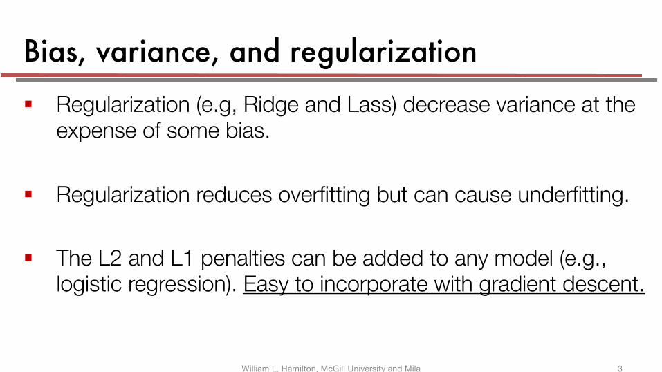
§ Regularization (e.g, Ridge and Lass) decrease variance at the expense of some bias.
§ Regularization reduces overfitting but can cause underfitting.
§ The L2 and L1 penalties can be added to any model (e.g., logistic regression). Easy to incorporate with gradient descent.
3
The concept of inductive bias
William L. Hamilton, McGill University and Mila
§ Statistical “bias” is not a bad thing in ML!§ It is all about having the right inductive bias. § ML is all about coming up with different models that
have different inductive biases. § Optional reading: “The Need for Biases in Learning
Generalizations"
4
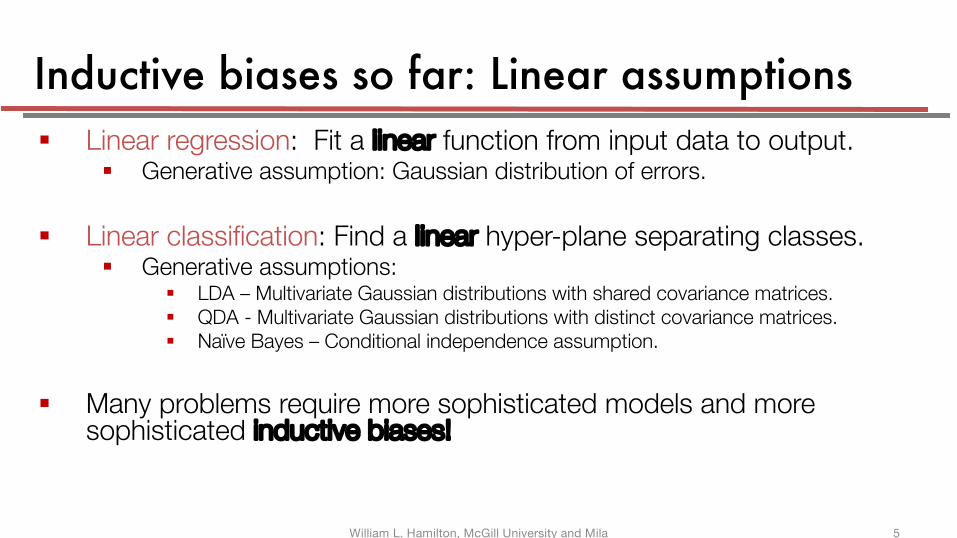
Inductive biases so far: Linear assumptions§ Linear regression: Fit a linear function from input data to output.
§ Generative assumption: Gaussian distribution of errors.
§ Linear classification: Find a linear hyper-plane separating classes.§ Generative assumptions:
§ LDA – Multivariate Gaussian distributions with shared covariance matrices.§ QDA - Multivariate Gaussian distributions with distinct covariance matrices.§ Naïve Bayes – Conditional independence assumption.
§ Many problems require more sophisticated models and more sophisticated inductive biases!
William L. Hamilton, McGill University and Mila 5
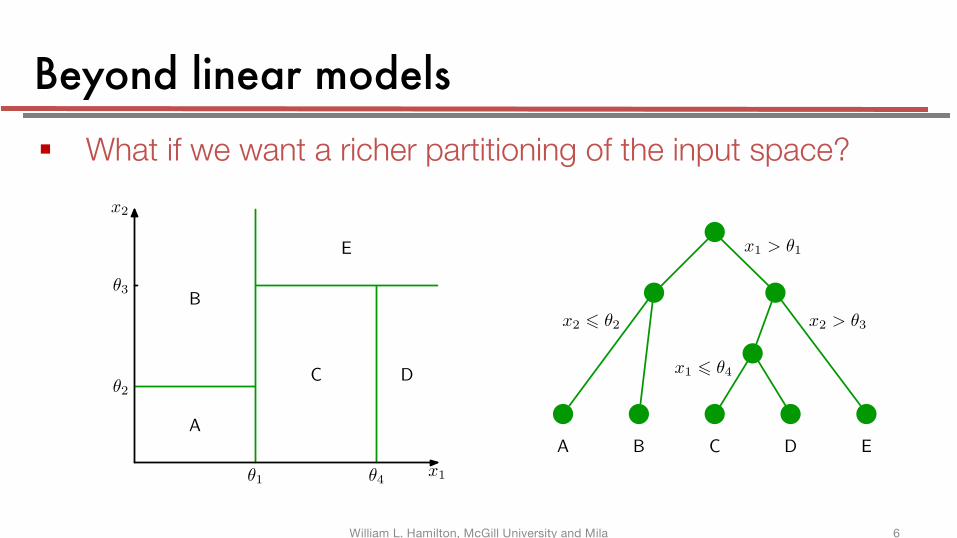
Beyond linear models§ What if we want a richer partitioning of the input space?
14.4. Tree-based Models 663
Figure 14.4 Comparison of the squared error(green) with the absolute error (red)showing how the latter places muchless emphasis on large errors andhence is more robust to outliers andmislabelled data points.
0 z
E(z)
−1 1
can be addressed by basing the boosting algorithm on the absolute deviation |y − t|instead. These two error functions are compared in Figure 14.4.
14.4. Tree-based Models
There are various simple, but widely used, models that work by partitioning theinput space into cuboid regions, whose edges are aligned with the axes, and thenassigning a simple model (for example, a constant) to each region. They can beviewed as a model combination method in which only one model is responsiblefor making predictions at any given point in input space. The process of selectinga specific model, given a new input x, can be described by a sequential decisionmaking process corresponding to the traversal of a binary tree (one that splits intotwo branches at each node). Here we focus on a particular tree-based frameworkcalled classification and regression trees, or CART (Breiman et al., 1984), althoughthere are many other variants going by such names as ID3 and C4.5 (Quinlan, 1986;Quinlan, 1993).
Figure 14.5 shows an illustration of a recursive binary partitioning of the inputspace, along with the corresponding tree structure. In this example, the first step
Figure 14.5 Illustration of a two-dimensional in-put space that has been partitionedinto five regions using axis-alignedboundaries.
A
B
C D
E
θ1 θ4
θ2
θ3
x1
x2
664 14. COMBINING MODELS
Figure 14.6 Binary tree corresponding to the par-titioning of input space shown in Fig-ure 14.5.
x1 > θ1
x2 > θ3
x1 ! θ4
x2 ! θ2
A B C D E
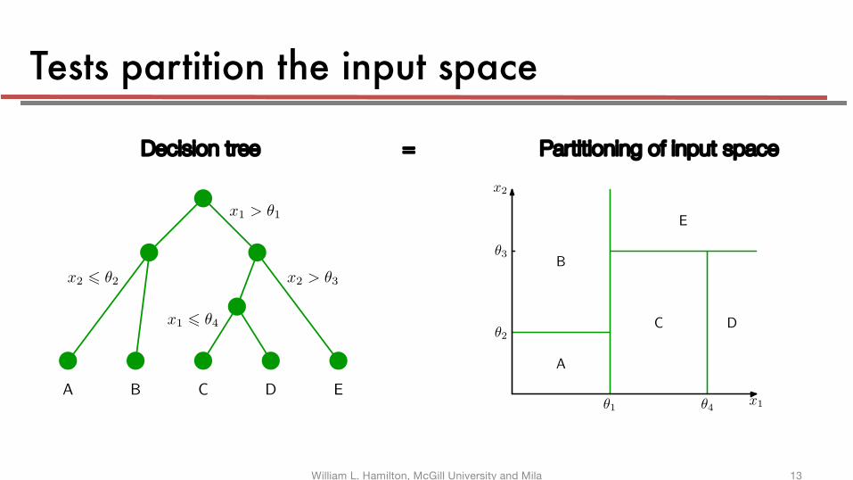
divides the whole of the input space into two regions according to whether x1 ! θ1
or x1 > θ1 where θ1 is a parameter of the model. This creates two subregions, eachof which can then be subdivided independently. For instance, the region x1 ! θ1
is further subdivided according to whether x2 ! θ2 or x2 > θ2, giving rise to theregions denoted A and B. The recursive subdivision can be described by the traversalof the binary tree shown in Figure 14.6. For any new input x, we determine whichregion it falls into by starting at the top of the tree at the root node and followinga path down to a specific leaf node according to the decision criteria at each node.Note that such decision trees are not probabilistic graphical models.
Within each region, there is a separate model to predict the target variable. Forinstance, in regression we might simply predict a constant over each region, or inclassification we might assign each region to a specific class. A key property of tree-based models, which makes them popular in fields such as medical diagnosis, forexample, is that they are readily interpretable by humans because they correspondto a sequence of binary decisions applied to the individual input variables. For in-stance, to predict a patient’s disease, we might first ask “is their temperature greaterthan some threshold?”. If the answer is yes, then we might next ask “is their bloodpressure less than some threshold?”. Each leaf of the tree is then associated with aspecific diagnosis.
In order to learn such a model from a training set, we have to determine thestructure of the tree, including which input variable is chosen at each node to formthe split criterion as well as the value of the threshold parameter θi for the split. Wealso have to determine the values of the predictive variable within each region.
Consider first a regression problem in which the goal is to predict a single targetvariable t from a D-dimensional vector x = (x1, . . . , xD)T of input variables. Thetraining data consists of input vectors {x1, . . . ,xN} along with the correspondingcontinuous labels {t1, . . . , tN}. If the partitioning of the input space is given, and weminimize the sum-of-squares error function, then the optimal value of the predictivevariable within any given region is just given by the average of the values of tn forthose data points that fall in that region.Exercise 14.10
Now consider how to determine the structure of the decision tree. Even for afixed number of nodes in the tree, the problem of determining the optimal structure(including choice of input variable for each split as well as the corresponding thresh-
William L. Hamilton, McGill University and Mila 6
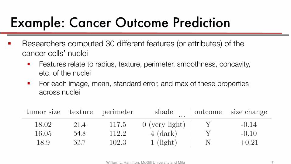
Example: Cancer Outcome Prediction§ Researchers computed 30 different features (or attributes) of the
cancer cells’ nuclei
§ Features relate to radius, texture, perimeter, smoothness, concavity, etc. of the nuclei
§ For each image, mean, standard error, and max of these properties across nuclei
tumor size texture perimeter shade outcome size change
18.02 rough 117.5 0 (very light) Y -0.1416.05 smooth 112.2 4 (dark) Y -0.1018.9 smooth 102.3 1 (light) N +0.21
21.454.832.7
…
William L. Hamilton, McGill University and Mila 7
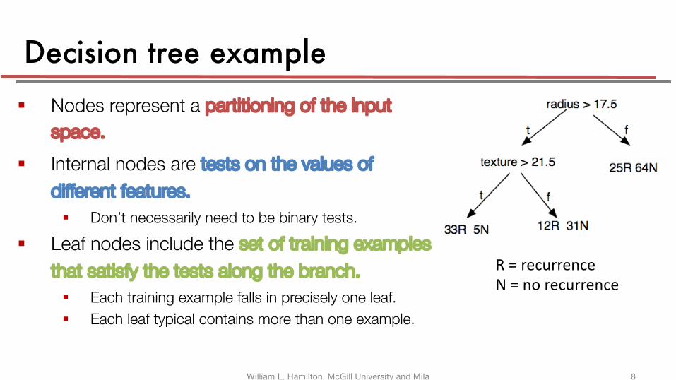
Decision tree example§ Nodes represent a partitioning of the input
space.
§ Internal nodes are tests on the values of
different features.
§ Don’t necessarily need to be binary tests.
§ Leaf nodes include the set of training examples
that satisfy the tests along the branch.
§ Each training example falls in precisely one leaf.
§ Each leaf typical contains more than one example.
R = recurrenceN = no recurrence
William L. Hamilton, McGill University and Mila 8
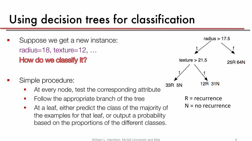
Using decision trees for classification
§ Suppose we get a new instance: radius=18, texture=12, …How do we classify it?
§ Simple procedure:§ At every node, test the corresponding attribute§ Follow the appropriate branch of the tree§ At a leaf, either predict the class of the majority of
the examples for that leaf, or output a probability based on the proportions of the different classes.
R = recurrenceN = no recurrence
William L. Hamilton, McGill University and Mila 9
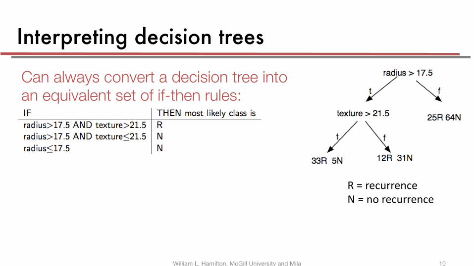
Interpreting decision trees
R = recurrenceN = no recurrence
Can always convert a decision tree into an equivalent set of if-then rules:
William L. Hamilton, McGill University and Mila 10
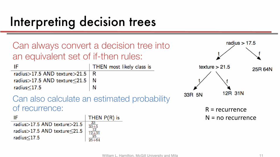
Interpreting decision trees
R = recurrenceN = no recurrence
Can always convert a decision tree into an equivalent set of if-then rules:
Can also calculate an estimated probability of recurrence:
William L. Hamilton, McGill University and Mila 11
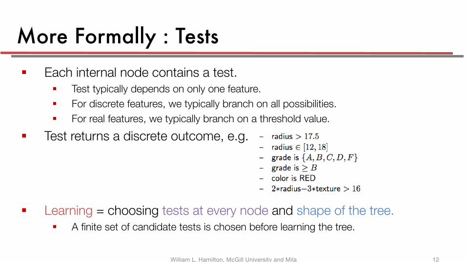
More Formally : Tests§ Each internal node contains a test.
§ Test typically depends on only one feature.
§ For discrete features, we typically branch on all possibilities.
§ For real features, we typically branch on a threshold value.
§ Test returns a discrete outcome, e.g.
§ Learning = choosing tests at every node and shape of the tree.§ A finite set of candidate tests is chosen before learning the tree.
William L. Hamilton, McGill University and Mila 12
Tests partition the input space
14.4. Tree-based Models 663
Figure 14.4 Comparison of the squared error(green) with the absolute error (red)showing how the latter places muchless emphasis on large errors andhence is more robust to outliers andmislabelled data points.
0 z
E(z)
−1 1
can be addressed by basing the boosting algorithm on the absolute deviation |y − t|instead. These two error functions are compared in Figure 14.4.
14.4. Tree-based Models
There are various simple, but widely used, models that work by partitioning theinput space into cuboid regions, whose edges are aligned with the axes, and thenassigning a simple model (for example, a constant) to each region. They can beviewed as a model combination method in which only one model is responsiblefor making predictions at any given point in input space. The process of selectinga specific model, given a new input x, can be described by a sequential decisionmaking process corresponding to the traversal of a binary tree (one that splits intotwo branches at each node). Here we focus on a particular tree-based frameworkcalled classification and regression trees, or CART (Breiman et al., 1984), althoughthere are many other variants going by such names as ID3 and C4.5 (Quinlan, 1986;Quinlan, 1993).
Figure 14.5 shows an illustration of a recursive binary partitioning of the inputspace, along with the corresponding tree structure. In this example, the first step
Figure 14.5 Illustration of a two-dimensional in-put space that has been partitionedinto five regions using axis-alignedboundaries.
A
B
C D
E
θ1 θ4
θ2
θ3
x1
x2
664 14. COMBINING MODELS
Figure 14.6 Binary tree corresponding to the par-titioning of input space shown in Fig-ure 14.5.
x1 > θ1
x2 > θ3
x1 ! θ4
x2 ! θ2
A B C D E
divides the whole of the input space into two regions according to whether x1 ! θ1
or x1 > θ1 where θ1 is a parameter of the model. This creates two subregions, eachof which can then be subdivided independently. For instance, the region x1 ! θ1
is further subdivided according to whether x2 ! θ2 or x2 > θ2, giving rise to theregions denoted A and B. The recursive subdivision can be described by the traversalof the binary tree shown in Figure 14.6. For any new input x, we determine whichregion it falls into by starting at the top of the tree at the root node and followinga path down to a specific leaf node according to the decision criteria at each node.Note that such decision trees are not probabilistic graphical models.
Within each region, there is a separate model to predict the target variable. Forinstance, in regression we might simply predict a constant over each region, or inclassification we might assign each region to a specific class. A key property of tree-based models, which makes them popular in fields such as medical diagnosis, forexample, is that they are readily interpretable by humans because they correspondto a sequence of binary decisions applied to the individual input variables. For in-stance, to predict a patient’s disease, we might first ask “is their temperature greaterthan some threshold?”. If the answer is yes, then we might next ask “is their bloodpressure less than some threshold?”. Each leaf of the tree is then associated with aspecific diagnosis.
In order to learn such a model from a training set, we have to determine thestructure of the tree, including which input variable is chosen at each node to formthe split criterion as well as the value of the threshold parameter θi for the split. Wealso have to determine the values of the predictive variable within each region.
Consider first a regression problem in which the goal is to predict a single targetvariable t from a D-dimensional vector x = (x1, . . . , xD)T of input variables. Thetraining data consists of input vectors {x1, . . . ,xN} along with the correspondingcontinuous labels {t1, . . . , tN}. If the partitioning of the input space is given, and weminimize the sum-of-squares error function, then the optimal value of the predictivevariable within any given region is just given by the average of the values of tn forthose data points that fall in that region.Exercise 14.10
Now consider how to determine the structure of the decision tree. Even for afixed number of nodes in the tree, the problem of determining the optimal structure(including choice of input variable for each split as well as the corresponding thresh-
Decision tree = Partitioning of input space
William L. Hamilton, McGill University and Mila 13
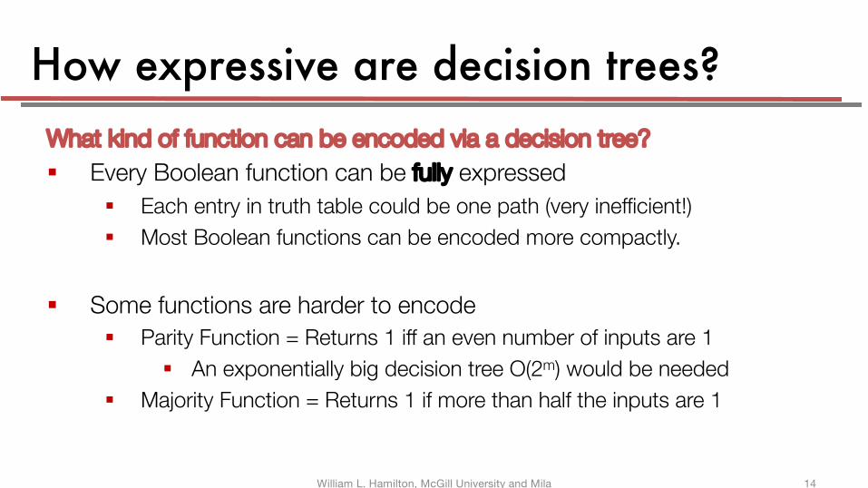
How expressive are decision trees?What kind of function can be encoded via a decision tree?§ Every Boolean function can be fully expressed
§ Each entry in truth table could be one path (very inefficient!)§ Most Boolean functions can be encoded more compactly.
§ Some functions are harder to encode§ Parity Function = Returns 1 iff an even number of inputs are 1
§ An exponentially big decision tree O(2m) would be needed§ Majority Function = Returns 1 if more than half the inputs are 1
William L. Hamilton, McGill University and Mila 14
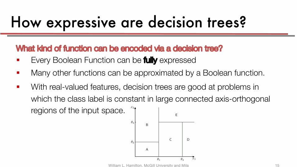
How expressive are decision trees?What kind of function can be encoded via a decision tree?
§ Every Boolean Function can be fully expressed
§ Many other functions can be approximated by a Boolean function.
§ With real-valued features, decision trees are good at problems in
which the class label is constant in large connected axis-orthogonal
regions of the input space.
14.4. Tree-based Models 663
Figure 14.4 Comparison of the squared error(green) with the absolute error (red)showing how the latter places muchless emphasis on large errors andhence is more robust to outliers andmislabelled data points.
0 z
E(z)
−1 1
can be addressed by basing the boosting algorithm on the absolute deviation |y − t|instead. These two error functions are compared in Figure 14.4.
14.4. Tree-based Models
There are various simple, but widely used, models that work by partitioning theinput space into cuboid regions, whose edges are aligned with the axes, and thenassigning a simple model (for example, a constant) to each region. They can beviewed as a model combination method in which only one model is responsiblefor making predictions at any given point in input space. The process of selectinga specific model, given a new input x, can be described by a sequential decisionmaking process corresponding to the traversal of a binary tree (one that splits intotwo branches at each node). Here we focus on a particular tree-based frameworkcalled classification and regression trees, or CART (Breiman et al., 1984), althoughthere are many other variants going by such names as ID3 and C4.5 (Quinlan, 1986;Quinlan, 1993).
Figure 14.5 shows an illustration of a recursive binary partitioning of the inputspace, along with the corresponding tree structure. In this example, the first step
Figure 14.5 Illustration of a two-dimensional in-put space that has been partitionedinto five regions using axis-alignedboundaries.
A
B
C D
E
θ1 θ4
θ2
θ3
x1
x2
William L. Hamilton, McGill University and Mila 15
Learning decision trees§ We could enumerate all possible trees (assuming the number of
possible tests is finite)
§ Each tree could be evaluated using the training set or, better yet, a validation set.
§ There are many possible trees! We would probably overfit the data….
§ Usually, decision trees are constructed in two phases:
1. A recursive, top-down procedure “grows” a tree (possibly until the training data is completely fit).
2. The tree is “pruned” back to avoid overfitting.
William L. Hamilton, McGill University and Mila 16
Top-down (recursive) induction of decision trees Given a set of labeled training instances:
1. If all the training instances have the same class, create a leaf with that class label and exit.
Else2. Pick the best test to split the data on.3. Split the training set according to the value of the outcome of the test.4. Recursively repeat steps 1 - 3 on each subset of the training data.
How do we pick the best test?
William L. Hamilton, McGill University and Mila 17
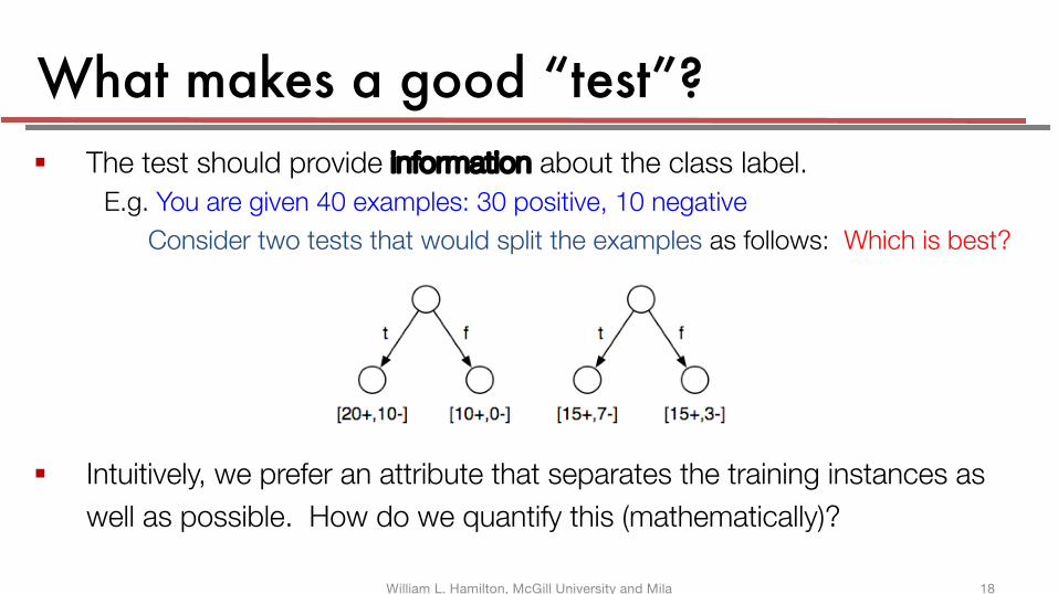
What makes a good “test”?§ The test should provide information about the class label.
E.g. You are given 40 examples: 30 positive, 10 negativeConsider two tests that would split the examples as follows: Which is best?
§ Intuitively, we prefer an attribute that separates the training instances as well as possible. How do we quantify this (mathematically)?
William L. Hamilton, McGill University and Mila 18
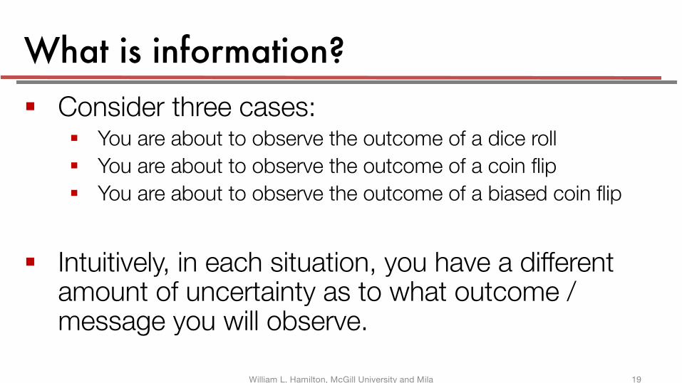
What is information?§ Consider three cases:
§ You are about to observe the outcome of a dice roll
§ You are about to observe the outcome of a coin flip
§ You are about to observe the outcome of a biased coin flip
§ Intuitively, in each situation, you have a different amount of uncertainty as to what outcome / message you will observe.
William L. Hamilton, McGill University and Mila 19
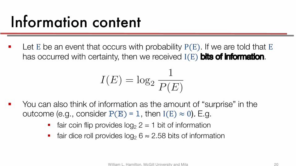
Information content § Let E be an event that occurs with probability P(E). If we are told that E
has occurred with certainty, then we received I(E) bits of information.
§ You can also think of information as the amount of “surprise” in the outcome (e.g., consider P(E) = 1, then I(E)≈0). E.g.
§ fair coin flip provides log2 2 = 1 bit of information
§ fair dice roll provides log2 6 ≈ 2.58 bits of information
I(E) = log21
P (E)
William L. Hamilton, McGill University and Mila 20
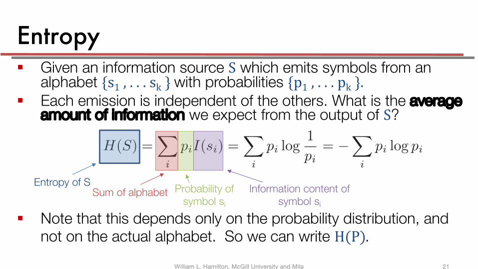
Entropy§ Given an information source S which emits symbols from an
alphabet {s1 ,...sk }with probabilities {p1 ,...pk }.§ Each emission is independent of the others. What is the average
amount of information we expect from the output of S?
§ Note that this depends only on the probability distribution, and not on the actual alphabet. So we can write H(P).
H(S) =X
i
piI(si) =X
i
pi log1
pi= �
X
i
pi log pi
Entropy of SSum of alphabet Probability of
symbol si
Information content of symbol si
William L. Hamilton, McGill University and Mila 21
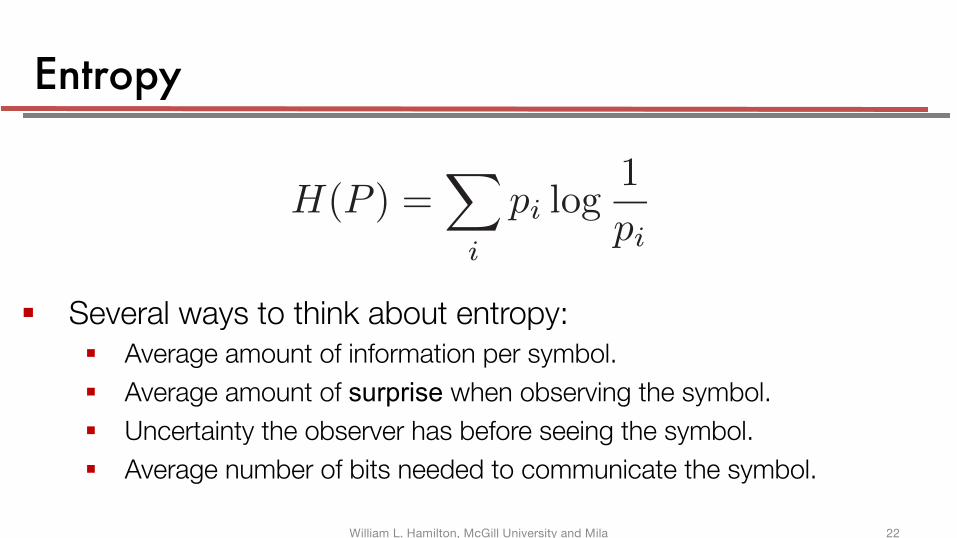
Entropy
§ Several ways to think about entropy:§ Average amount of information per symbol.
§ Average amount of surprise when observing the symbol.
§ Uncertainty the observer has before seeing the symbol.
§ Average number of bits needed to communicate the symbol.
H(P ) =X
i
pi log1
pi
William L. Hamilton, McGill University and Mila 22
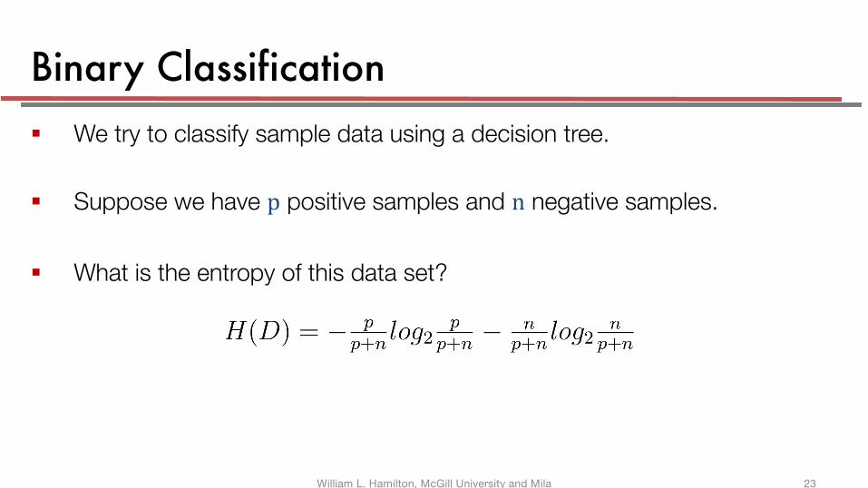
Binary Classification§ We try to classify sample data using a decision tree.
§ Suppose we have p positive samples and n negative samples.
§ What is the entropy of this data set?
William L. Hamilton, McGill University and Mila 23
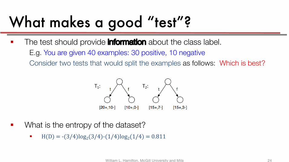
§ The test should provide information about the class label.
E.g. You are given 40 examples: 30 positive, 10 negative
Consider two tests that would split the examples as follows: Which is best?
§ What is the entropy of the dataset?
§ H(D)=-(3/4)log2(3/4)-(1/4)log2(1/4)=0.811
What makes a good “test”?
T1: T2:
William L. Hamilton, McGill University and Mila 24

Conditional entropy
§ The conditional entropy, H(y|x),is the average specific conditional entropy of y given the values of x:
§ Interpretation: The expected number of bits needed to transmit y if both the emitter and receiver know x.
Example: Conditional entropy
x =HasKids y =OwnsDumboVideo
Yes Yes
Yes Yes
Yes Yes
Yes Yes
No No
No No
Yes No
Yes No
Specific conditional entropy is the uncertainty in y given a particular xvalue. E.g.,
• P (y = Y ES|x = Y ES) = 23, P (y = NO|x = Y ES) = 1
3
• H(y|x = Y ES) = 23 log
1(23)
+ 13 log
1(13)
⌥ 0.9183.
COMP-652, Lecture 8 - October 2, 2012 27
Conditional entropy
• The conditional entropy, H(y|x), is the average specific conditional
entropy of y given the values for x:
H(y|x) =X
v
P (x = v)H(y|x = v)
• E.g. (from previous slide),
– H(y|x = Y ES) = 23 log
1(23)
+ 13 log
1(13)
⌥ 0.6365
– H(y|x = NO) = 0 log 10 + 1 log 1
1 = 0.– H(y|x) = H(y|x = Y ES)P (x = Y ES) + H(y|x = NO)P (x =
NO) = 0.6365 ⇤ 34 + 0 ⇤ 1
4 ⌥ 0.4774
• Interpretation: the expected number of bits needed to transmit y if both
the emitter and the receiver know the possible values of x (but before
they are told x’s specific value).
COMP-652, Lecture 8 - October 2, 2012 28
William L. Hamilton, McGill University and Mila 25
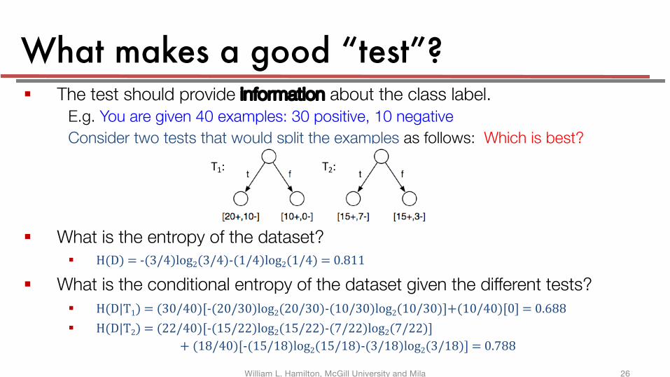
§ The test should provide information about the class label.E.g. You are given 40 examples: 30 positive, 10 negative
Consider two tests that would split the examples as follows: Which is best?
§ What is the entropy of the dataset? § H(D)=-(3/4)log2(3/4)-(1/4)log2(1/4)=0.811
§ What is the conditional entropy of the dataset given the different tests?§ H(D|T1)=(30/40)[-(20/30)log2(20/30)-(10/30)log2(10/30)]+(10/40)[0]=0.688§ H(D|T2)=(22/40)[-(15/22)log2(15/22)-(7/22)log2(7/22)]
+(18/40)[-(15/18)log2(15/18)-(3/18)log2(3/18)]=0.788
What makes a good “test”?
T1: T2:
William L. Hamilton, McGill University and Mila 26
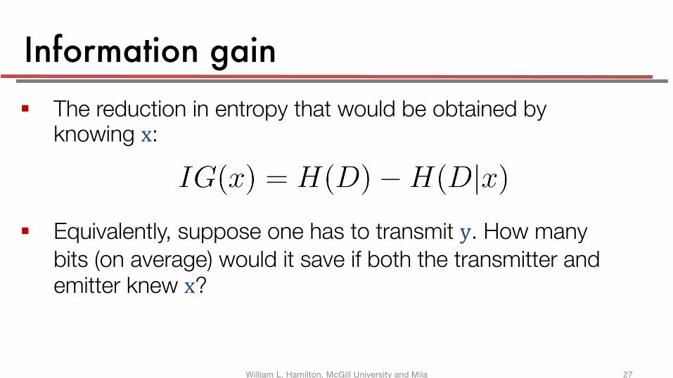
Information gain § The reduction in entropy that would be obtained by
knowing x:
§ Equivalently, suppose one has to transmit y. How many bits (on average) would it save if both the transmitter and emitter knew x?
William L. Hamilton, McGill University and Mila 27
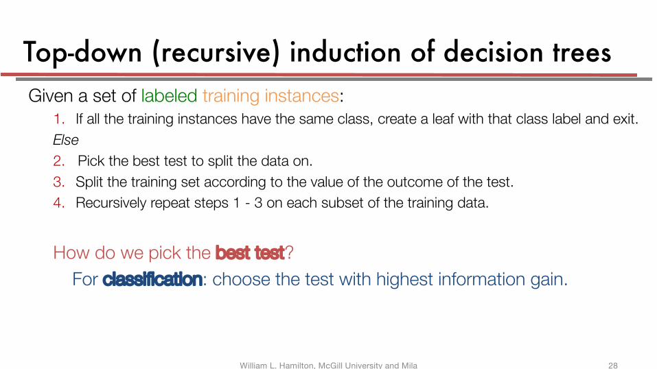
Top-down (recursive) induction of decision trees Given a set of labeled training instances:
1. If all the training instances have the same class, create a leaf with that class label and exit. Else2. Pick the best test to split the data on.3. Split the training set according to the value of the outcome of the test.4. Recursively repeat steps 1 - 3 on each subset of the training data.
How do we pick the best test?For classification: choose the test with highest information gain.
William L. Hamilton, McGill University and Mila 28
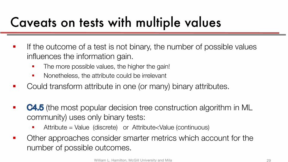
Caveats on tests with multiple values
§ If the outcome of a test is not binary, the number of possible values influences the information gain.§ The more possible values, the higher the gain!§ Nonetheless, the attribute could be irrelevant
§ Could transform attribute in one (or many) binary attributes.
§ C4.5 (the most popular decision tree construction algorithm in ML community) uses only binary tests: § Attribute = Value (discrete) or Attribute<Value (continuous)
§ Other approaches consider smarter metrics which account for the number of possible outcomes.
William L. Hamilton, McGill University and Mila 29
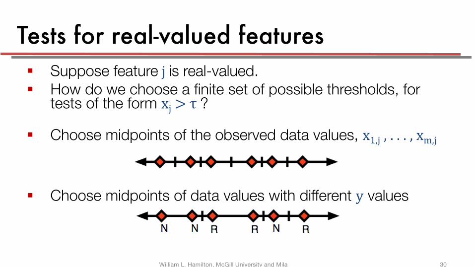
Tests for real-valued features § Suppose feature jis real-valued.§ How do we choose a finite set of possible thresholds, for
tests of the form xj >τ ?
§ Choose midpoints of the observed data values, x1,j ,...,xm,j
§ Choose midpoints of data values with different y values
William L. Hamilton, McGill University and Mila 30
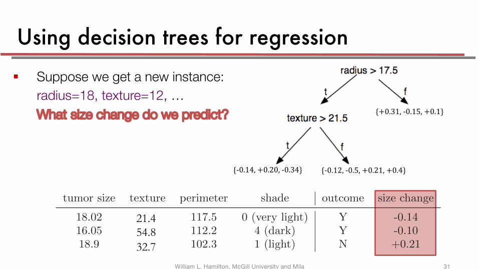
Using decision trees for regression
§ Suppose we get a new instance:
radius=18, texture=12, …
What size change do we predict?
tumor size texture perimeter shade outcome size change
18.02 rough 117.5 0 (very light) Y -0.1416.05 smooth 112.2 4 (dark) Y -0.1018.9 smooth 102.3 1 (light) N +0.21
21.454.832.7
{-0.14,+0.20,-0.34} {-0.12,-0.5,+0.21,+0.4}
{+0.31,-0.15,+0.1}
William L. Hamilton, McGill University and Mila 31
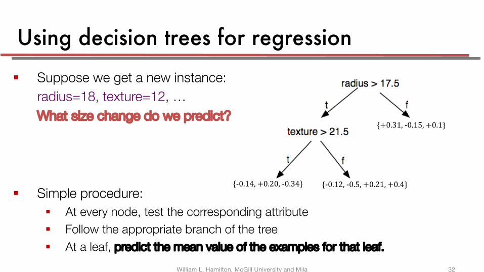
Using decision trees for regression
§ Suppose we get a new instance:
radius=18, texture=12, …
What size change do we predict?
§ Simple procedure:
§ At every node, test the corresponding attribute
§ Follow the appropriate branch of the tree
§ At a leaf, predict the mean value of the examples for that leaf.
{-0.14,+0.20,-0.34} {-0.12,-0.5,+0.21,+0.4}
{+0.31,-0.15,+0.1}
William L. Hamilton, McGill University and Mila 32

Top-down (recursive) induction of decision trees Given a set of labeled training instances:
1. If all the training instances have the same class, create a leaf with that class label and exit. Else2. Pick the best test to split the data on.3. Split the training set according to the value of the outcome of the test.4. Recursively repeat steps 1 - 3 on each subset of the training data.
How do we pick the best test?For classification: choose the test with highest information gain.
For regression: choose the test with lowest mean-squared error.
William L. Hamilton, McGill University and Mila 33
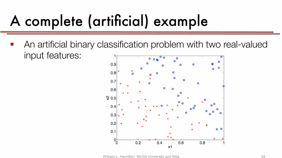
A complete (artificial) example § An artificial binary classification problem with two real-valued
input features:
William L. Hamilton, McGill University and Mila 34
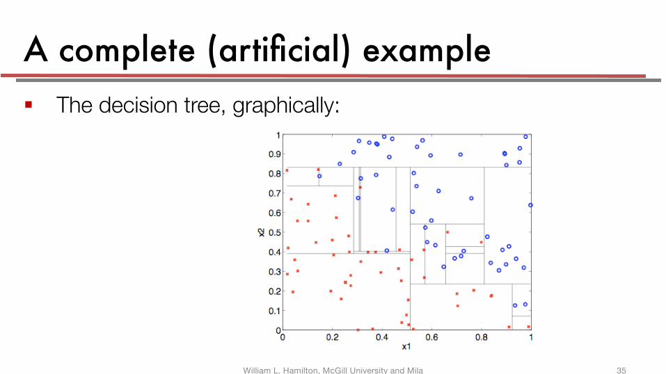
A complete (artificial) example§ The decision tree, graphically:
William L. Hamilton, McGill University and Mila 35

0.4
0.5
0.6
0.7
0.8
0.9
1
0 20 40 60 80 100
Pro
po
rtio
n c
orr
ect
on
tes
t se
t
Training set size
Assessing performance
§ Split data into a training set and a validation set
§ Apply learning algorithm to training set.
§ Measure error with the validation set.
William L. Hamilton, McGill University and Mila 36
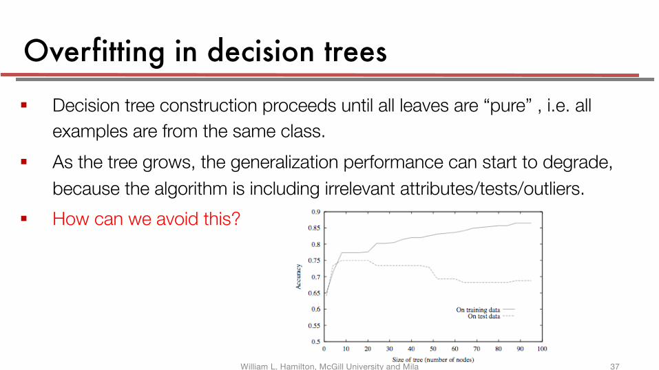
Overfitting in decision trees
§ Decision tree construction proceeds until all leaves are “pure” , i.e. all examples are from the same class.
§ As the tree grows, the generalization performance can start to degrade, because the algorithm is including irrelevant attributes/tests/outliers.
§ How can we avoid this?
William L. Hamilton, McGill University and Mila 37
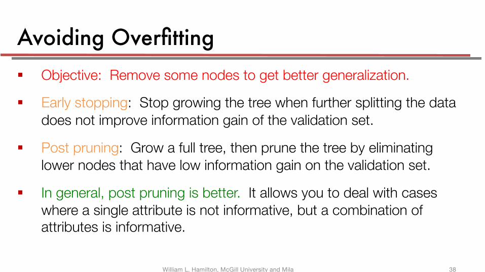
Avoiding Overfitting§ Objective: Remove some nodes to get better generalization.
§ Early stopping: Stop growing the tree when further splitting the data does not improve information gain of the validation set.
§ Post pruning: Grow a full tree, then prune the tree by eliminating lower nodes that have low information gain on the validation set.
§ In general, post pruning is better. It allows you to deal with cases where a single attribute is not informative, but a combination of attributes is informative.
William L. Hamilton, McGill University and Mila 38
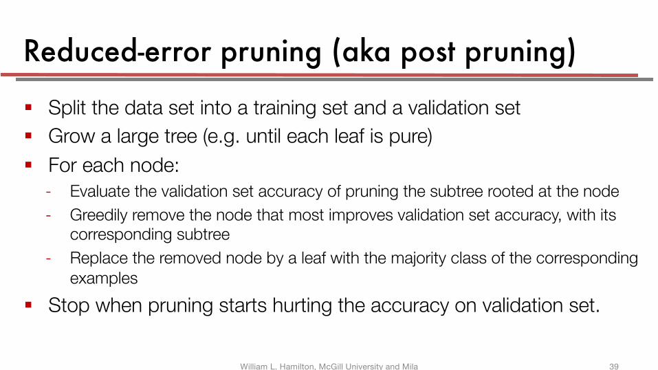
Reduced-error pruning (aka post pruning)
§ Split the data set into a training set and a validation set
§ Grow a large tree (e.g. until each leaf is pure)
§ For each node:- Evaluate the validation set accuracy of pruning the subtree rooted at the node
- Greedily remove the node that most improves validation set accuracy, with its corresponding subtree
- Replace the removed node by a leaf with the majority class of the corresponding examples
§ Stop when pruning starts hurting the accuracy on validation set.
William L. Hamilton, McGill University and Mila 39
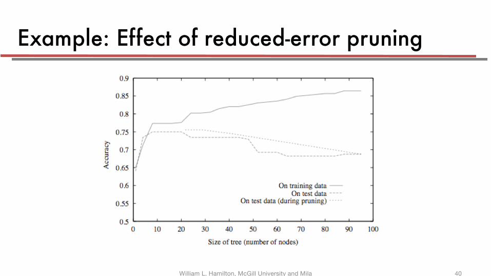
Example: Effect of reduced-error pruning
William L. Hamilton, McGill University and Mila 40
Advantages of decision trees
§ Provide a general representation of classification rules§ Scaling / normalization not needed, as we use no notion of “distance”
between examples.
§ The learned function, y=f(x), is easy to interpret.
§ Fast learning algorithms (e.g. C4.5, CART).
§ Good accuracy in practice – many applications in industry!
William L. Hamilton, McGill University and Mila 41
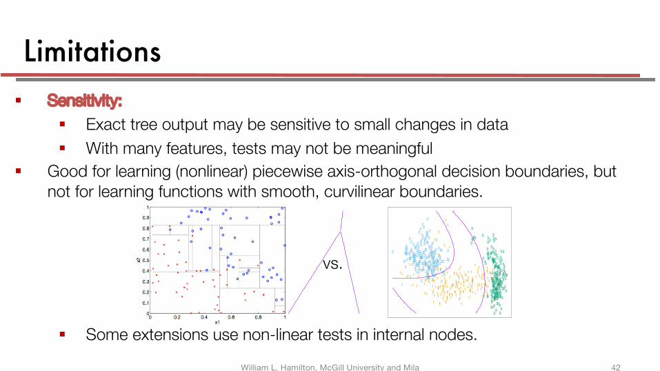
Limitations§ Sensitivity:
§ Exact tree output may be sensitive to small changes in data
§ With many features, tests may not be meaningful
§ Good for learning (nonlinear) piecewise axis-orthogonal decision boundaries, but not for learning functions with smooth, curvilinear boundaries.
§ Some extensions use non-linear tests in internal nodes.
12
Joelle Pineau 23
Using higher-order features 4.2 Linear Regression of an Indicator Matrix 103
1
1
1
1111
11
11
1
1
1
1
1
1
11 1
111
1
1
1
1
1
11
1
1
11
1
11
11
1
1
1
1
1
1
1 11
1
1 1
1
1
1
1
1
1
111
1
1
1
1
1
1
1 111
1
1
1
11
1
1
1
1
1
11
1
1
1
11
1
1
1
1
111
1
1
11
11
1
1
1
1
1
11
1
1
1
1
1
1 1
1
1
11
1
1
1
1 1
1
1
11 1
1
1
1 11
11
1
1
1
1
1
1
1
11
1 1
11
1
1
1
11
1
1
1
1 1
11
1
11
1
1
1
1
11
1
11
1
11
1
1
111
1
1 1
1
11
1
1
11
1
1
1
1
1
1
1
1
1
1
22
222
2
2
2
22
2
222
22
2
22
222
2
222
2
2
2
2 2
2
2
2
22
2
2
22
2
2
2
2
2
2 222
2
2
2
2
2
22
2
2
22
2
2
2
2
2
2
2
2
2
2
22
2
2
2
2
2
2
2
2
22
2
2
222
2
2
2
2
2 2
2
2
2
2
2
22
2
2
2
2 22
2
2
2
2
2
2
2
2
2
2
2
2 22
2
2
2
2
2
2
2
22
2
2
2
22
2 2
22 2
2
2
2
2
2
2
2
2
2
2
2
22
2
22
222
2
2
2
222
2
2
2
2
2
2
2
2
2
2
2
2
2
2
2
2
2
2
2
2
2
2
2 22
2
2
22
22
2 2
2
2
2
3
3
3
3
33
3
3
3
3
3 3
3
3
3
3
3
3
3
3
3
33
3
3
3
33
3
33
3
3
3
3
3
3
3
3 3
3
3
3
3
33
3
3
33
3
3
33
3
333
3
3
3 3
3 3
3
3
3
3
3
3
3
3
3
3
33
3 3
3
33
3 3
33
3
3
3
333
3
3
3
3
3
3
3
3
33
3
3
3
3 3
3
3
3
33
3
3 33
3
3
33
3
3
3
3
3
3
3
3
3
3
3
3
3
33
3
33
33
3
33
3
3
3
3
3
3
3 3
3
3
3 3
3
3
3
33
3
3
3 3
33
33
3
3
3
3
3
3
3
3
3
3
3
3
33
3
3
3
3
3
3
3
3
3
3
3
3
3
3
3
3
3
3
3
1
1
1
1111
11
11
1
1
1
1
1
1
11 1
111
1
1
1
1
1
11
1
1
11
1
11
11
1
1
1
1
1
1
1 11
1
1 1
1
1
1
1
1
1
111
1
1
1
1
1
1
1 111
1
1
1
11
1
1
1
1
1
11
1
1
1
11
1
1
1
1
111
1
1
11
11
1
1
1
1
1
11
1
1
1
1
1
1 1
1
1
11
1
1
1
1 1
1
1
11 1
1
1
1 11
11
1
1
1
1
1
1
1
11
1 1
11
1
1
1
11
1
1
1
1 1
11
1
11
1
1
1
1
11
1
11
1
11
1
1
111
1
1 1
1
11
1
1
11
1
1
1
1
1
1
1
1
1
1
22
222
2
2
2
22
2
222
22
2
22
222
2
222
2
2
2
2 2
2
2
2
22
2
2
22
2
2
2
2
2
2 222
2
2
2
2
2
22
2
2
22
2
2
2
2
2
2
2
2
2
2
22
2
2
2
2
2
2
2
2
22
2
2
222
2
2
2
2
2 2
2
2
2
2
2
22
2
2
2
2 22
2
2
2
2
2
2
2
2
2
2
2
2 22
2
2
2
2
2
2
2
22
2
2
2
22
2 2
22 2
2
2
2
2
2
2
2
2
2
2
2
22
2
22
222
2
2
2
222
2
2
2
2
2
2
2
2
2
2
2
2
2
2
2
2
2
2
2
2
2
2
2 22
2
2
22
22
2 2
2
2
2
3
3
3
3
33
3
3
3
3
3 3
3
3
3
3
3
3
3
3
3
33
3
3
3
33
3
33
3
3
3
3
3
3
3
3 3
3
3
3
3
33
3
3
33
3
3
33
3
333
3
3
3 3
3 3
3
3
3
3
3
3
3
3
3
3
33
3 3
3
33
3 3
33
3
3
3
333
3
3
3
3
3
3
3
3
33
3
3
3
3 3
3
3
3
33
3
3 33
3
3
33
3
3
3
3
3
3
3
3
3
3
3
3
3
33
3
33
33
3
33
3
3
3
3
3
3
3 3
3
3
3 3
3
3
3
33
3
3
3 3
33
33
3
3
3
3
3
3
3
3
3
3
3
3
33
3
3
3
3
3
3
3
3
3
3
3
3
3
3
3
3
3
3
3
FIGURE 4.1. The left plot shows some data from three classes, with lineardecision boundaries found by linear discriminant analysis. The right plot showsquadratic decision boundaries. These were obtained by finding linear boundariesin the five-dimensional space X1, X2, X1X2, X
21 , X
22 . Linear inequalities in this
space are quadratic inequalities in the original space.
mation h(X) where h : IRp !→ IRq with q > p, and will be explored in laterchapters.
4.2 Linear Regression of an Indicator Matrix
Here each of the response categories are coded via an indicator variable.Thus if G has K classes, there will be K such indicators Yk, k = 1, . . . ,K,with Yk = 1 if G = k else 0. These are collected together in a vectorY = (Y1, . . . , YK), and the N training instances of these form an N × Kindicator response matrix Y. Y is a matrix of 0’s and 1’s, with each rowhaving a single 1. We fit a linear regression model to each of the columnsof Y simultaneously, and the fit is given by
Y = X(XTX)−1XTY. (4.3)
Chapter 3 has more details on linear regression. Note that we have a coeffi-cient vector for each response column yk, and hence a (p+1)×K coefficientmatrix B = (XTX)−1XTY. Here X is the model matrix with p+1 columnscorresponding to the p inputs, and a leading column of 1’s for the intercept.
A new observation with input x is classified as follows:
• compute the fitted output f(x)T = (1, xT )B, a K vector;
• identify the largest component and classify accordingly:
G(x) = argmaxk∈G fk(x). (4.4)
COMP-598: Applied Machine Learning
Joelle Pineau 24
Quadratic discriminant analysis
• LDA assumes all classes have the same covariance matrix, Σ.
• QDA allows different covariance matrices, Σy for each class y.
• Linear discriminant function:
• Quadratic discriminant function:
– QDA has more parameters to estimate, but greater flexibility to estimate the target function. Bias-variance trade-off.
COMP-598: Applied Machine Learning
δy (x) = xTΣ−1µy −
12µyTΣ−1µy + logP(y)
δy (x) = −12Σy −
12(x −µy )
T Σy−1(x −µy )+ logP(y)
vs.
William L. Hamilton, McGill University and Mila 42
What you should know§ How to use a decision tree to classify a new example.
§ How to build a decision tree using an information-theoretic approach.
§ How to detect (and fix) overfitting in decision trees.
§ How to handle both discrete and continuous attributes and outputs.
William L. Hamilton, McGill University and Mila 43