April 2007

NASA/TP-2007-214869

Cohesive Elements for Shells Carlos G. Dávila NASA Langley Research Center, Hampton, Virginia Pedro P. Camanho University of Porto, Porto, Portugal Albert Turon University of Girona, Girona, Spain

https://ntrs.nasa.gov/search.jsp?R=20070018344 2018-05-07T14:08:36+00:00Z

The NASA STI Program Office ... in Profile

Since its founding, NASA has been dedicated to the advancement of aeronautics and space science. The NASA Scientific and Technical Information (STI) Program Office plays a key part in helping NASA maintain this important role. The NASA STI Program Office is operated by Langley Research Center, the lead center for NASA’s scientific and technical information. The NASA STI Program Office provides access to the NASA STI Database, the largest collection of aeronautical and space science STI in the world. The Program Office is also NASA’s institutional mechanism for disseminating the results of its research and development activities. These results are published by NASA in the NASA STI Report Series, which includes the following report types: • TECHNICAL PUBLICATION. Reports of

completed research or a major significant phase of research that present the results of NASA programs and include extensive data or theoretical analysis. Includes compilations of significant scientific and technical data and information deemed to be of continuing reference value. NASA counterpart of peer-reviewed formal professional papers, but having less stringent limitations on manuscript length and extent of graphic presentations.

• TECHNICAL MEMORANDUM.

Scientific and technical findings that are preliminary or of specialized interest, e.g., quick release reports, working papers, and bibliographies that contain minimal annotation. Does not contain extensive analysis.

• CONTRACTOR REPORT. Scientific and

technical findings by NASA-sponsored contractors and grantees.

• CONFERENCE PUBLICATION. Collected papers from scientific and technical conferences, symposia, seminars, or other meetings sponsored or co-sponsored by NASA.

• SPECIAL PUBLICATION. Scientific,

technical, or historical information from NASA programs, projects, and missions, often concerned with subjects having substantial public interest.

• TECHNICAL TRANSLATION. English-

language translations of foreign scientific and technical material pertinent to NASA’s mission.

Specialized services that complement the STI Program Office’s diverse offerings include creating custom thesauri, building customized databases, organizing and publishing research results ... even providing videos. For more information about the NASA STI Program Office, see the following: • Access the NASA STI Program Home

Page at http://www.sti.nasa.gov • E-mail your question via the Internet to

help@sti.nasa.gov • Fax your question to the NASA STI Help

Desk at (301) 621-0134 • Telephone the NASA STI Help Desk at

(301) 621-0390 • Write to:

NASA STI Help Desk NASA Center for AeroSpace Information 7115 Standard Drive Hanover, MD 21076-1320

April 2007

NASA/TP-2007-214869

Cohesive Elements for Shells Carlos G. Dávila NASA Langley Research Center, Hampton, Virginia Pedro P. Camanho University of Porto, Porto, Portugal Albert Turon University of Girona, Girona, Spain

National Aeronautics and Space Administration NASA Langley Research Center Hampton, VA 23681

Available from:

NASA Center for AeroSpace Information National Technical Information Service 7115 Standard Drive 5285 Port Royal Road Hanover, MD 21076-1320 Springfield, VA 22161 301-621-0390 703-605-6000

1

Abstract

A cohesive element for shell analysis is presented. The element can be used to simulate the initiation and growth of delaminations between stacked, non-coincident layers of shell elements. The procedure to construct the element accounts for the thickness offset by applying the kinematic relations of shell deformation to transform the stiffness and internal force of a zero-thickness cohesive element such that interfacial continuity between the layers is enforced. The procedure is demonstrated by simulating the response and failure of the Mixed Mode Bending test and a skin-stiffener debond specimen. In addition, it is shown that stacks of shell elements can be used to create effective models to predict the inplane and delamination failure modes of thick components. The results indicate that simple shell models can retain many of the necessary predictive attributes of much more complex 3D models while providing the computational efficiency that is necessary for design.

Keywords: cohesive elements; shell elements; delamination; composite laminates

Nomenclature

a = crack length A = area of integration of cohesive element B = strain-displacement matrix C = constitutive matrix D = damage matrix d = damage variable e = length of lever arm in MMB test F = applied force FShell = internal force of shell cohesive element F3D = internal force of zero-thickness cohesive element GI, GII, GIII = mode I, II, and III energy release rates Gc = critical energy release rate GIc, GIIc = critical energy release rates in mode I, II GT = total energy release rate I = identity matrix J = J-integral K = penalty stiffness for cohesive law KShell = stiffness matrix of shell cohesive element K3D = stiffness matrix of zero-thickness cohesive element

2

lele = element length Rij, R = shell transformation matrices S = stress tensor s, t = pseudo time factor t

F = pseudo time factor at the maximum load t j = thickness of j-th ply t

u, t l = thickness of the plies above and below an interface

jD3

U , jShell

U = vector of degrees of freedom at a node for 3D and shell cohesive elements

D3U , ShellU = vector of all degrees of freedom of 3D and shell cohesive elements

uj, vj, wj, xjθ , yjθ = translational and rotational nodal degrees of freedom

αij = coefficients of thermal expansion 0Δ = displacement jump for damage initiation fΔ = final displacement jump 213 ,, ΔΔΔ = mode I, mode II, and mode III displacement jumps

shearΔ = tangential displacement jump

ΔT = difference between the curing temperature and room temperature ijδ = Kronecker delta

λ = equivalent displacement jump ρ = viscoelastic regularization factor η = parameter of Benzeggagh-Kenane mixed-mode fracture criterion τ, τi = interfacial tractions 00

3 , shearττ = nominal peel and shear strengths

**3 , shearττ = reduced peel and shear strengths

Introduction

Delamination is one of the predominant modes of failure in laminated composites when there is no reinforcement in the thickness direction. In order to design structures that are flaw- and damage-tolerant, analyses must be conducted to study the propagation of delaminations. The calculation of delaminations can be performed using cohesive elements1, 2, which combine aspects of strength-based analysis to predict the onset of damage at the interface, and fracture mechanics to predict the propagation of a delamination.

Cohesive elements are normally designed to represent the separation at the zero-thickness interface between layers of three-dimensional elements (3D). Unfortunately, the softening laws that govern the debonding of the plies often result in extremely slow convergence rates for the solution procedure, and require very refined meshes in the region ahead of the crack tip. In addition, it is often difficult to model zero-thickness interfaces using conventional finite element pre-processors.

The typical requirement of extremely fine meshes ahead of the crack tip1, 3, 4 has been recently relaxed by a procedure that artificially reduces the interfacial strength while keeping the fracture energy constant

3

in order to increase the length of the cohesive zone. A longer cohesive zone allows the use of larger cohesive elements3. However, the difficulties associated with the generation of complex meshes composed of stacks of 3D elements joined together with zero-thickness cohesive elements often render the use of cohesive elements impractical outside research environments.

Shell elements are more efficient for modeling thin-walled structures than 3D elements. Shell finite element analysis has been used in conjunction with the Virtual Crack Closure Technique (VCCT) by Wang et al.5, 6 to evaluate strain energy release rates for the damage tolerance analysis of skin-stiffener interfaces. Wang used a wall offset to move the nodes from the reference surfaces to a coincident location on the interface between the skin and the flange. Therefore, compatibility was ensured by equating the three translational degrees of freedom of both shells with constraint equations and by allowing the rotations to be free. These models were shown to require a fraction of the degrees of freedom than are needed for full 3D analyses while producing accurate values for mode I and mode II strain energy release rates.

However, Glaessgen et al.7 observed that shell VCCT models of debond specimens in which the adherends are of different thickness predict the correct total energy release rate but that the mode mixity does not converge with mesh refinement. This phenomenon is similar to the well known oscillatory behavior of the in-plane linear elastic stress field near the tip of a bi-material interfacial crack8.

Very few references discuss the use of shell models in combination with cohesive elements and most of them are designed for explicit time integration. A shell model for discrete delaminations under mode I loading using finite-thickness volumetric elements connecting shell elements was proposed by Reedy9. Johnson et al.10 applied the bilinear traction-displacement of the Crisfield11 cohesive model in conjunction with the Ladevèze mesomodel12 for intralaminar damage to investigate wing leading edge impact and crash response of composite structures. A mixed-mode adhesive contact shell element that accounts for the thickness offset and the rotational degrees of freedom in the shells was developed by Borg13 for the explicit finite element code LS-DYNA®. Bruno et al.14 developed shell models that use rigid links to offset the location of the cohesive element nodes from the shell reference surface to the interface between the layers. Using this technique, multi-layered shell models were analyzed using the zero-thickness cohesive elements available in the commercial finite element code LUSAS®.

Cohesive elements have been found useful to study fracture along bi-metallic interfaces15-18. Cohesive laws eliminate the stress singularity at the delamination front and, consequently, they prevent the oscillation in the stress field and the corresponding non-convergence of fracture mode mixity18. Therefore, it is expected that the non-convergence of the mode mixity observed by Glaessgen in shell VCCT models, which is also caused by a mismatch of the elastic stiffnesses of the adherends, is also avoided in cohesive models. However, a study of the mesh independence of mode mixity in cohesive shell models has not been attempted by the present authors.

The objective of this work is to present a method for the construction of shell cohesive elements for implicit analysis. The formulation of an 8-node cohesive element for modeling delamination between shell elements on the basis of a 3D cohesive element previously developed by the authors1, 2 is proposed. The formulation takes into account the rotational degrees of freedom at the shell nodes and the relative location of the interface which allows the construction of models with more than one layer of cohesive interfaces and does not require coincident nodes along an interface nor does it require the use of rigid links. Therefore, the formulation allows the use of several layers of shell/cohesive elements through the thickness of a thick laminate. Since the cohesive elements have the topology of a standard 8-node element, the models are simpler to generate than those based on zero-thickness interfaces.

In the following sections, the constitutive damage model previously developed by the authors will be outlined. Then, a procedure to construct a shell cohesive element from that of any conventional zero-thickness cohesive element will be described. Finally, three different examples of increasing structural complexity will be presented to show that simple shell models based on the proposed cohesive element for shells can be used to represent the onset and propagation of delamination in structural components.

4

Bilinear Cohesive Law

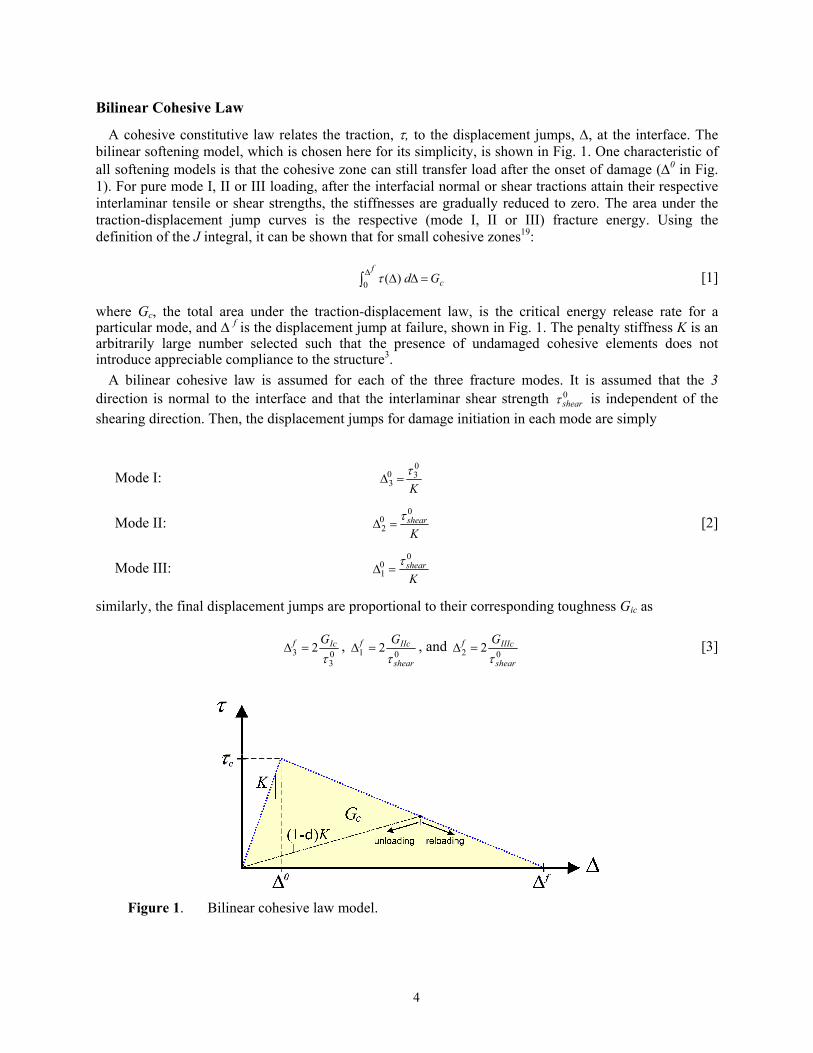
A cohesive constitutive law relates the traction, τ, to the displacement jumps, Δ, at the interface. The bilinear softening model, which is chosen here for its simplicity, is shown in Fig. 1. One characteristic of all softening models is that the cohesive zone can still transfer load after the onset of damage (Δ0 in Fig. 1). For pure mode I, II or III loading, after the interfacial normal or shear tractions attain their respective interlaminar tensile or shear strengths, the stiffnesses are gradually reduced to zero. The area under the traction-displacement jump curves is the respective (mode I, II or III) fracture energy. Using the definition of the J integral, it can be shown that for small cohesive zones19:

cf

Gd =ΔΔ∫Δ 0 )(τ [1]

where Gc, the total area under the traction-displacement law, is the critical energy release rate for a particular mode, and Δ f is the displacement jump at failure, shown in Fig. 1. The penalty stiffness K is an arbitrarily large number selected such that the presence of undamaged cohesive elements does not introduce appreciable compliance to the structure3.

A bilinear cohesive law is assumed for each of the three fracture modes. It is assumed that the 3 direction is normal to the interface and that the interlaminar shear strength 0

shearτ is independent of the shearing direction. Then, the displacement jumps for damage initiation in each mode are simply

Mode I: K

030

3τ

=Δ

Mode II: K

shear0

02

τ=Δ [2]

Mode III: K

shear0

01

τ=Δ

similarly, the final displacement jumps are proportional to their corresponding toughness Gic as

03

3 2τ

Icf G=Δ ,

01 2shear

IIcf Gτ

=Δ , and 02 2shear

IIIcf Gτ

=Δ [3]

Figure 1. Bilinear cohesive law model.

5

Cohesive Law for Mixed-Mode Delamination

In structural applications of composites, delamination growth is likely to occur under mixed-mode loading. Therefore, a general formulation for cohesive elements must deal with mixed-mode delamination growth problems.

Under pure mode I, II or III loading, the onset of damage at the interface can be determined simply by comparing the tractions with their respective allowable. Under mixed-mode loading, however, damage onset may occur before any of the traction components involved reach their respective allowable. Therefore, a mixed-mode criterion must be established in terms of an interaction between components of the energy release rate.

The constitutive damage model used here, formulated in the context of Damage Mechanics (DM), was previously proposed by the authors2. The damage model simulates delamination onset and delamination propagation using a single scalar variable, d, to track the damage at the interface under general loading conditions. An initiation criterion that evolves from the Benzeggagh–Kenane fracture criterion20 (B-K) ensures that the model accounts for changes in the loading mode in a thermodynamically consistent way and avoids restoration of the cohesive state.

The constitutive model prevents interpenetration of the faces of the crack during closing, and a Fracture Mechanics-based criterion is used to predict crack propagation. The parameter λ is the norm of the displacement jump tensor (also called equivalent displacement jump norm), and it is used to compare different stages of the displacement jump state so that it is possible to define such concepts as ‘loading’, ‘unloading’ and ‘reloading’. The equivalent displacement jump is a non-negative and continuous function, defined as:

( )223 shearΔ+Δ=λ [4]

where >⋅< is the MacAuley bracket defined as ( )xxx +>=< 21 , which sets any negative values to zero.

The term Δ3 is the displacement jump in mode I, i.e., normal to the mid-plane, and Δshear is the tangential displacement calculated as the Euclidean norm of the displacement jump in mode II and in mode III:

( )22

21 Δ+Δ=Δshear [5]

A bilinear cohesive law for mixed-mode delamination can be constructed by determining the initial damage threshold Δ0 from the criterion for damage initiation and the final displacement jump, Δf, from the formulation of the propagation surface or propagation criterion2. For the B-K fracture criterion, the mixed-mode displacement jump for damage initiation is2

( ) ( ) ( )η

⎟⎟⎠

⎞⎜⎜⎝

⎛ +⎟⎠⎞⎜

⎝⎛ Δ−Δ+Δ=Δ

T

IIIIIshear G

GG203

20203

0 [6]

where the B-K parameter η is obtained by curve-fitting the fracture toughness of mixed-mode tests and the fracture mode ratio is2

ββ

β221 2

2

−+=⎟⎟

⎠

⎞⎜⎜⎝

⎛ +

T

IIIII

GGG [7]

where the displacement jump ratio is defined as ( )3/ Δ+ΔΔ= shearshearβ .

6

The displacement jump for final fracture is also obtained from the critical displacement jumps as

0

303

03

03 )(

Δ

⎟⎟⎠

⎞⎜⎜⎝

⎛ +ΔΔ−ΔΔ+ΔΔ

=Δ

η

T

IIIIIffshearshear

f

f GGG

[8]

During overload, the state of damage d is a function of the current equivalent displacement jump λ :

( )( )0

0

Δ−ΔΔ−Δ

= f

f

λλd [9]

The corresponding tractions can be written as

jj

jjijjiji KD Δ

⎥⎥

⎦

⎤

⎢⎢

⎣

⎡

⎟⎟

⎠

⎞

⎜⎜

⎝

⎛

Δ

Δ−+−=Δ= 311 δδτ d [10]

where the Kronecker ijδ is used to prevent the interpenetration of the surfaces of a damaged element when contact occurs2.

In summary, by assuming that toughnesses and strengths in modes II and III are equal to each other, it is shown that the mixed-mode constitutive equations of a cohesive element are defined by five material properties and three displacement jumps: GIc, GIIc, 00

3 , shearττ , K, 321 and,, ΔΔΔ . This formulation of the damage model allows an explicit integration of the constitutive model and ensures consistency in the evolution of damage during loading, unloading, and changes in mode mixity. The derivation and implementation of the cohesive damage model is described in Refs. [2, 21] and the reader is referred to those sources for details that will not be repeated here.

Viscoelastic regularization

Material models exhibiting softening behavior and sharp stiffness degradation typically exhibit severe convergence difficulties in implicit analysis programs. To improve the convergence rate of the iterative procedure, a viscous regularization scheme was implemented as suggested by ABAQUS22 for its cohesive element and composite damage models. The procedure is a generalization of the Duvaut-Lions regularization model which, for sufficiently small time increments, maintains the tangent stiffness tensor of the softening material as positive definite. Defining d as the “kinematic” damage that depends on the displacement variables and dv as the “regularized” damage variable, the rate of change in the damage variable dv is a function of the damping factor ρ:

( )vv ddd −=ρ1& [11]

The regularized damage variable at time t+Δt is updated as

t

vtttt

ttt

v ddd Δ+Δ+Δ+Δ

Δ++= ρ

ρρ [12]

It can be observed that the viscoelastic factor has the units of time and, therefore, its effect depends on the pseudo-time load proportionality factor which is selected arbitrarily by the user. In the following

7

sections, the effect of the pseudo-time on the viscoelastic factor is eliminated by specifying it as a nondimensional value, Ft/ρ , where Ft is the estimated pseudo-time at the maximum load.

The response of the damaged material is evaluated using the regularized damage variables. Using viscous regularization with a viscosity parameter that is much smaller than the time increment can improve the rate of convergence in the presence of softening processes without compromising the accuracy of the results. However, the use of larger values of the regularization parameter can cause a toughening of the material response and produce a stable propagation of delamination in problems with unstable delamination growth.

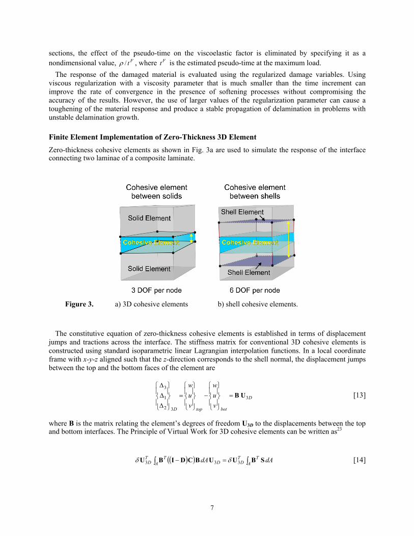
Finite Element Implementation of Zero-Thickness 3D Element Zero-thickness cohesive elements as shown in Fig. 3a are used to simulate the response of the interface connecting two laminae of a composite laminate.

Figure 3. a) 3D cohesive elements b) shell cohesive elements.

The constitutive equation of zero-thickness cohesive elements is established in terms of displacement

jumps and tractions across the interface. The stiffness matrix for conventional 3D cohesive elements is constructed using standard isoparametric linear Lagrangian interpolation functions. In a local coordinate frame with x-y-z aligned such that the z-direction corresponds to the shell normal, the displacement jumps between the top and the bottom faces of the element are

D

bottopD vuw

vuw

3

32

1

3

UB=⎪⎭

⎪⎬

⎫

⎪⎩

⎪⎨

⎧−

⎪⎭

⎪⎬

⎫

⎪⎩

⎪⎨

⎧=

⎪⎭

⎪⎬

⎫

⎪⎩

⎪⎨

⎧

ΔΔΔ

[13]

where B is the matrix relating the element’s degrees of freedom U3D to the displacements between the top and bottom interfaces. The Principle of Virtual Work for 3D cohesive elements can be written as23

( )( ) dAdA ATT

DDATT

D SBUUBCDIBU ∫∫ =− 333 δδ [14]

8

where D is a diagonal matrix composed the damage state d at the interface. The term I represents the identity matrix, and C is the undamaged constitutive matrix whose diagonal is composed of the penalty stiffnesses K, and S is the stress tensor. The stiffness matrix K3D of the element is easily identified in the left hand side of Eq. 14 as the integral over the area A of the element:

( )( ) dAAT

D BCDIBK ∫ −=3 [15]

and the right hand side of Eq. 14 provides the element’s internal force:

dAAT

D SBF ∫=3 [16]

Because the stiffness K3D is constructed from the displacements U3D, only three degrees of freedom can be active at a node, i.e., u, v, and w. The integration of the terms in Eqs. 15 and 16 is performed numerically using either Newton-Cotes or Gaussian integration. The element proposed is implemented in ABAQUS22 as a user-defined element.

Formulation Shell Cohesive Element

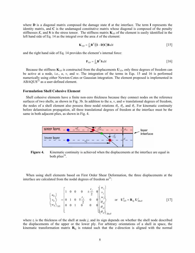
Shell cohesive elements have a finite non-zero thickness because they connect nodes on the reference surfaces of two shells, as shown in Fig. 3b. In addition to the u, v, and w translational degrees of freedom, the nodes of a shell element also possess three nodal rotations θx, θy, and θz. For kinematic continuity before delamination propagation, all three translational degrees of freedom at the interface must be the same in both adjacent plies, as shown in Fig. 4.

Figure 4. Kinematic continuity is achieved when the displacements at the interface are equal in both plies24.

When using shell elements based on First Order Shear Deformation, the three displacements at the interface are calculated from the nodal degrees of freedom as23:

jShellkj

kD

Shellzj

yj

xj

j

j

j

j

j

Dk

k

k wvu

t

t

wvu

URU =

⎪⎪⎪⎪

⎭

⎪⎪⎪⎪

⎬

⎫

⎪⎪⎪⎪

⎩

⎪⎪⎪⎪

⎨

⎧

⎥⎥⎥⎥⎥⎥⎥

⎦

⎤

⎢⎢⎢⎢⎢⎢⎢

⎣

⎡±

=⎪⎭

⎪⎬

⎫

⎪⎩

⎪⎨

⎧

3

3

or

000100

002

010

02

0001

θθθ

m [17]

where tj is the thickness of the shell at node j, and its sign depends on whether the shell node described the displacements of the upper or the lower ply. For arbitrary orientations of a shell in space, the kinematic transformation matrix Rkj is rotated such that the z-direction is aligned with the normal

9

direction defined by two connected shell nodes. A transformation matrix R for the entire set of degrees of freedom in an element can be assembled using the transformations Rkj such that

ShellDShellD URUURU δδ == 33 and [18]

The stiffness matrix Kshell of a cohesive element for shell analysis can be constructed by substituting Eqs. 18 into the expression of the Principle of Virtual Work for a 3D cohesive element (Eq. 12):

( )( ) dAdA ATTT

ShellShellATTT

Shell SBRUURBCDIBRU ∫∫ =− δδ [19]

By comparing Eqs. 14 and 19, it is clear that the stiffness and internal force of a shell cohesive element can be constructed from any standard cohesive element formulation using the following expressions:

DT

ShellDT

Shell 33 and FRFRKRK == [20]

Eqs. 20 show that a cohesive element for shells is easily constructed from any 3D cohesive element by simple matrix multiplication. An 8-node cohesive element for shells was implemented as an ABAQUS UEL (user element) subroutine22 by using a zero-thickness 3D element previously developed by the authors2 as a kernel.

Spatial Orientation of the Shell Normals

The transformations shown in Eqs. 20 is only valid when the normals to the upper and the lower shells are aligned with the z-direction of the global reference frame. In the case of arbitrary orientation of the shells in space, it is necessary to define local reference frames at each corner of the shell cohesive elements. In the present model, the local normal direction (z') is defined by the vector between the lower and upper nodes at a corner. Using a rotation tensor, the normal and tangential components of the displacement jump can be expressed in terms of the displacement field in global coordinates.

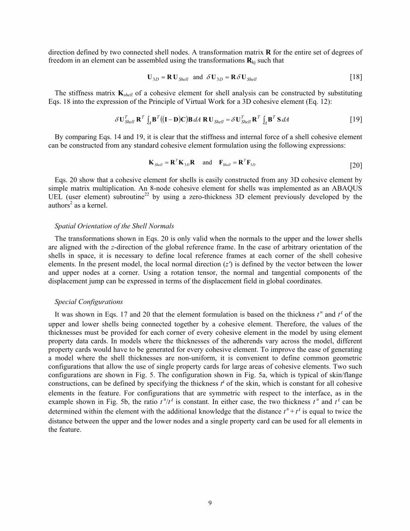
Special Configurations

It was shown in Eqs. 17 and 20 that the element formulation is based on the thickness t u and t

l of the upper and lower shells being connected together by a cohesive element. Therefore, the values of the thicknesses must be provided for each corner of every cohesive element in the model by using element property data cards. In models where the thicknesses of the adherends vary across the model, different property cards would have to be generated for every cohesive element. To improve the ease of generating a model where the shell thicknesses are non-uniform, it is convenient to define common geometric configurations that allow the use of single property cards for large areas of cohesive elements. Two such configurations are shown in Fig. 5. The configuration shown in Fig. 5a, which is typical of skin/flange constructions, can be defined by specifying the thickness t

l of the skin, which is constant for all cohesive elements in the feature. For configurations that are symmetric with respect to the interface, as in the example shown in Fig. 5b, the ratio t

u/t l is constant. In either case, the two thickness t

u and t l can be

determined within the element with the additional knowledge that the distance t u + t

l is equal to twice the distance between the upper and the lower nodes and a single property card can be used for all elements in the feature.

10

Figure 5. Special configurations with constant thickness properties.

Example and Verification Problems

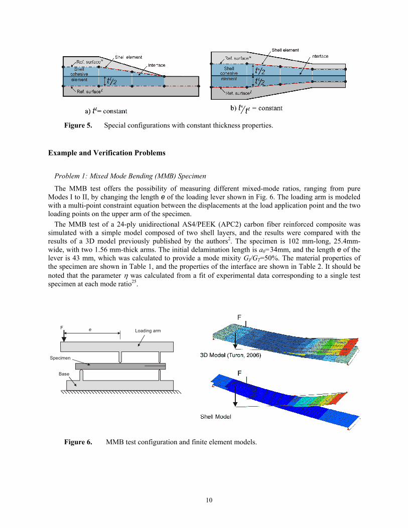
Problem 1: Mixed Mode Bending (MMB) Specimen

The MMB test offers the possibility of measuring different mixed-mode ratios, ranging from pure Modes I to II, by changing the length e of the loading lever shown in Fig. 6. The loading arm is modeled with a multi-point constraint equation between the displacements at the load application point and the two loading points on the upper arm of the specimen.

The MMB test of a 24-ply unidirectional AS4/PEEK (APC2) carbon fiber reinforced composite was simulated with a simple model composed of two shell layers, and the results were compared with the results of a 3D model previously published by the authors2. The specimen is 102 mm-long, 25.4mm- wide, with two 1.56 mm-thick arms. The initial delamination length is a0=34mm, and the length e of the lever is 43 mm, which was calculated to provide a mode mixity GI/GT=50%. The material properties of the specimen are shown in Table 1, and the properties of the interface are shown in Table 2. It should be noted that the parameter η was calculated from a fit of experimental data corresponding to a single test specimen at each mode ratio25.

e

Specimen

F Loading arm

Base

Figure 6. MMB test configuration and finite element models.

11

Table 1. Material Properties of AS4/Peek25.

E11 (GPa) E22=E33 (GPa) ν12=ν13 ν23 G12=G13 (GPa) G23 (GPa) 122.7 10.1 0.25 0.45 5.5 3.7

Table 2. Properties of the interface1, 25.

GIc (N/mm) GIIc (N/mm) 03τ (MPa) 0

shearτ (MPa) η 0.969 1.719 80 100 2.28

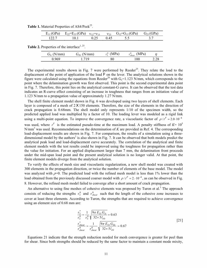
The experimental results shown in Fig. 7 were performed by Reeder25. They relate the load to the

displacement of the point of application of the load F on the lever. The analytical solutions shown in the figure were calculated using the equations from Reeder26 with Gc=1.123 N/mm, which corresponds to the point where the delamination growth was first observed. This point is the second experimental data point in Fig. 7. Therefore, this point lies on the analytical constant-G curve. It can be observed that the test data indicates an R-curve effect consisting of an increase in toughness that ranges from an initiation value of 1.123 N/mm to a propagation value of approximately 1.27 N/mm.

The shell finite element model shown in Fig. 6 was developed using two layers of shell elements. Each layer is composed of a mesh of 2 X 150 elements. Therefore, the size of the elements in the direction of crack propagation is 0.68mm. The shell model only represents 1/10 of the specimen width, so the predicted applied load was multiplied by a factor of 10. The loading lever was modeled as a rigid link using a multi-point equation. To improve the convergence rate, a viscoelastic factor of 4100.2/ −⋅=Ftρ was used, where Ft is the estimated pseudo-time at the maximum load. A penalty stiffness of K= 105 N/mm3 was used. Recommendations on the determination of K are provided in Ref. 4. The corresponding load-displacement results are shown in Fig. 7. For comparison, the results of a simulation using a three-dimensional model by the authors2 is also shown in Fig. 7. It can be observed that both models predict the analytical peak load and load-displacement curve accurately. The correlation of the analytical and finite element models with the test results could be improved using the toughness for propagation rather than the value for initiation. For an applied displacement larger than 7 mm, the delamination front proceeds under the mid-span load point and the present analytical solution is no longer valid. At that point, the finite element models diverge from the analytical solution.

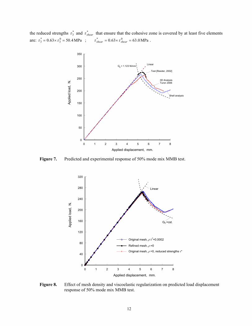
To verify the effects of mesh size and viscoelastic regularization, a new shell model was created with 300 elements in the propagation direction, or twice the number of elements of the base model. The model was analyzed with ρ=0. The predicted load with the refined mesh model is less than 1% lower than the load obtained from the previously discussed coarser model with 410.2/ −⋅=Ftρ , as can be observed in Fig. 8. However, the refined mesh model failed to converge after a short amount of crack propagation.

An alternative to using fine meshes of cohesive elements was proposed by Turon et al.3 The approach consists of reducing the strengths 0

3τ and 0shearτ such that the length of the cohesive zone increases to

cover at least three elements. According to Turon, the strengths that are required to achieve convergence using an element size of 0.68 mm are:

67.0

53291

63.0532

91

3300

*

3303

03

*3

=×

=

=×

=

ele

IIc

shearshear

shear

ele

Ic

lGE

lGE

πττ

τ

πττ

τ

[21]

Equations 21 indicate that the strength reduction needed for mesh convergence is greater for peel than for shear. Since both strengths should be reduced by the same factor to maintain a constant mode mixity,

12

the reduced strengths *3τ and *

shearτ that ensure that the cohesive zone is covered by at least five elements are: MPa0.6363.0 ; MPa4.5063.0 0*0

3*3 =×==×= shearshear ττττ .

0

50

100

150

200

250

300

350

0 1 2 3 4 5 6 7 8

Appl

ied

load

, N

.

Applied displacement, mm.

Linear

Test [Reeder, 2002]

Shell analysis

3D AnalysisTuron 2006

G = 1.123 N/mmc

Figure 7. Predicted and experimental response of 50% mode mix MMB test.

0

40

80

120

160

200

240

280

320

0 1 2 3 4 5 6 7 8

Appl

ied

load

, N

.

Applied displacement, mm.

G =cst.

Linear

Original mesh, ρ /tF=0.0002

Original mesh, ρ =0, reduced strengths τ*

Refined mesh, ρ =0

c

Figure 8. Effect of mesh density and viscoelastic regularization on predicted load displacement response of 50% mode mix MMB test.

13

An analysis was performed with the original (coarse) mesh model with reduced strengths and no viscoelastic regularization. The results shown in Fig. 8 indicate that the results from the original (coarser) mesh using reduced strengths are virtually identical to those using a refined mesh. In the present problem, the use of lowered strengths reduces the occurrence of divergence in the iterative solution and the use of viscoelastic regularization is not required.

Problem 2: Debonding of Skin-Stiffener Specimen

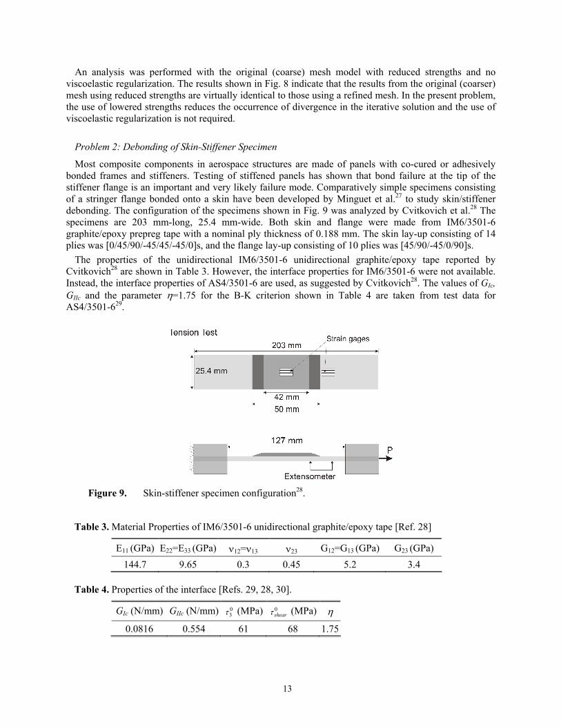
Most composite components in aerospace structures are made of panels with co-cured or adhesively bonded frames and stiffeners. Testing of stiffened panels has shown that bond failure at the tip of the stiffener flange is an important and very likely failure mode. Comparatively simple specimens consisting of a stringer flange bonded onto a skin have been developed by Minguet et al.27 to study skin/stiffener debonding. The configuration of the specimens shown in Fig. 9 was analyzed by Cvitkovich et al.28 The specimens are 203 mm-long, 25.4 mm-wide. Both skin and flange were made from IM6/3501-6 graphite/epoxy prepreg tape with a nominal ply thickness of 0.188 mm. The skin lay-up consisting of 14 plies was [0/45/90/-45/45/-45/0]s, and the flange lay-up consisting of 10 plies was [45/90/-45/0/90]s.

The properties of the unidirectional IM6/3501-6 unidirectional graphite/epoxy tape reported by Cvitkovich28 are shown in Table 3. However, the interface properties for IM6/3501-6 were not available. Instead, the interface properties of AS4/3501-6 are used, as suggested by Cvitkovich28. The values of GIc, GIIc and the parameter η=1.75 for the B-K criterion shown in Table 4 are taken from test data for AS4/3501-629.

Figure 9. Skin-stiffener specimen configuration28.

Table 3. Material Properties of IM6/3501-6 unidirectional graphite/epoxy tape [Ref. 28]

E11 (GPa) E22=E33 (GPa) ν12=ν13 ν23 G12=G13 (GPa) G23 (GPa) 144.7 9.65 0.3 0.45 5.2 3.4

Table 4. Properties of the interface [Refs. 29, 28, 30].

GIc (N/mm) GIIc (N/mm) 03τ (MPa) 0

shearτ (MPa) η

0.0816 0.554 61 68 1.75

14

A complete analysis of the delamination growth in the tension specimen requires a high degree of

complexity. For instance, Krueger31 developed highly detailed two-dimensional models using up to four elements per ply thickness. In previously published work30, the authors determined that it is possible to predict the debond load of the specimen using cohesive elements using a relatively coarse three-dimensional model. To keep the modeling difficulties low and the approach applicable to larger problems, the 3D model was developed using only two brick elements through the thickness of the skin, and another two through the flange. The complete model consists of 1,002 three-dimensional 8-node C3DI elements and 15,212 degrees of freedom. This model did not contain any pre-existing delaminations.

To account for the effect of residual thermal strains, a thermal analysis step was conducted before the mechanical loads were applied. The same coefficients of thermal expansion (α11=-2.4x10-8/ºC and α22=3.7x10-5/ºC) are applied to the skin and the flange, and the temperature difference between the curing and room temperature is ΔT= -157 ºC [Krueger31]. The flange has more 90º plies than 0º plies and the skin is quasi-orthotropic, so that residual thermal stresses develop at room temperature at the skin/flange interface.

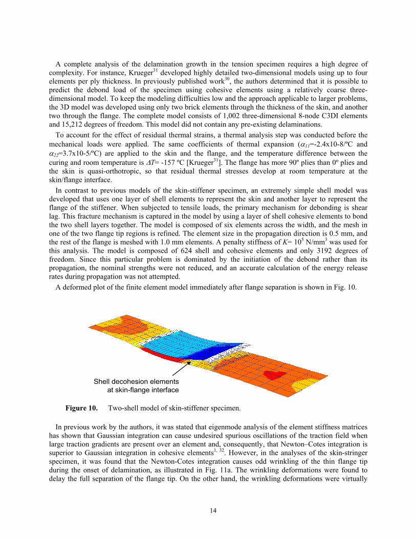
In contrast to previous models of the skin-stiffener specimen, an extremely simple shell model was developed that uses one layer of shell elements to represent the skin and another layer to represent the flange of the stiffener. When subjected to tensile loads, the primary mechanism for debonding is shear lag. This fracture mechanism is captured in the model by using a layer of shell cohesive elements to bond the two shell layers together. The model is composed of six elements across the width, and the mesh in one of the two flange tip regions is refined. The element size in the propagation direction is 0.5 mm, and the rest of the flange is meshed with 1.0 mm elements. A penalty stiffness of K= 105 N/mm3 was used for this analysis. The model is composed of 624 shell and cohesive elements and only 3192 degrees of freedom. Since this particular problem is dominated by the initiation of the debond rather than its propagation, the nominal strengths were not reduced, and an accurate calculation of the energy release rates during propagation was not attempted.

A deformed plot of the finite element model immediately after flange separation is shown in Fig. 10.

Shell decohesion elements at skin-flange interface

Figure 10. Two-shell model of skin-stiffener specimen.

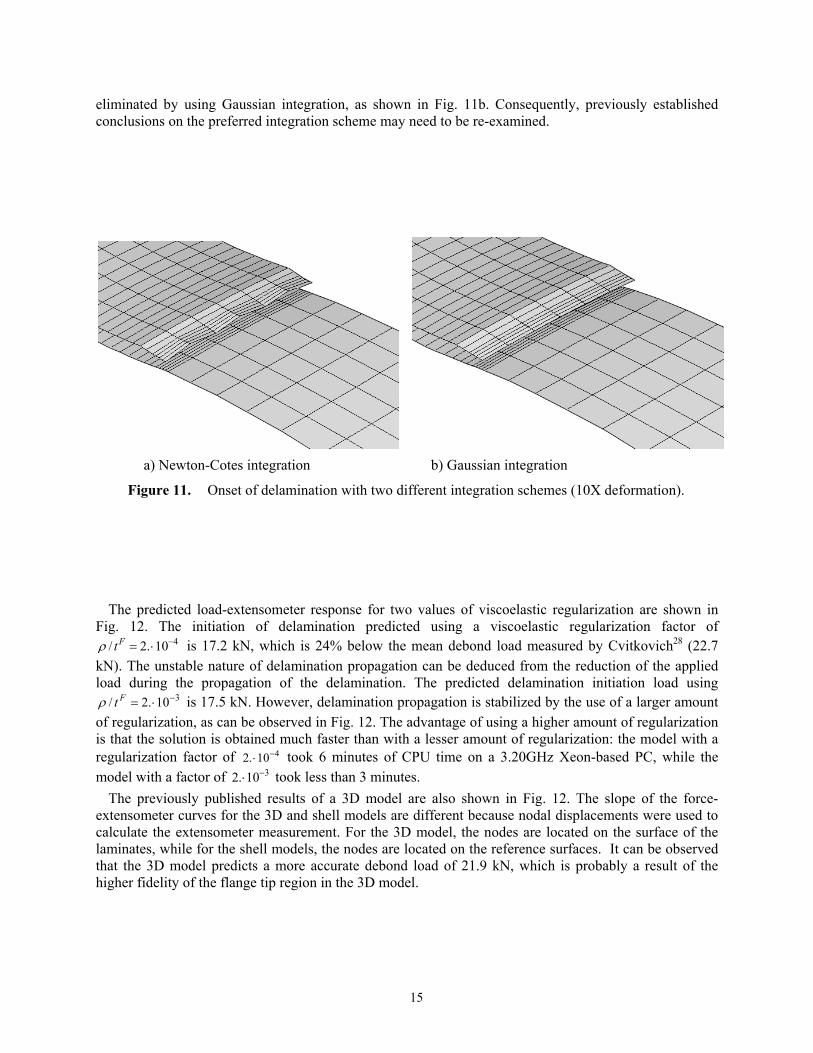
In previous work by the authors, it was stated that eigenmode analysis of the element stiffness matrices has shown that Gaussian integration can cause undesired spurious oscillations of the traction field when large traction gradients are present over an element and, consequently, that Newton–Cotes integration is superior to Gaussian integration in cohesive elements1, 32. However, in the analyses of the skin-stringer specimen, it was found that the Newton-Cotes integration causes odd wrinkling of the thin flange tip during the onset of delamination, as illustrated in Fig. 11a. The wrinkling deformations were found to delay the full separation of the flange tip. On the other hand, the wrinkling deformations were virtually

15

eliminated by using Gaussian integration, as shown in Fig. 11b. Consequently, previously established conclusions on the preferred integration scheme may need to be re-examined.

a) Newton-Cotes integration b) Gaussian integration

Figure 11. Onset of delamination with two different integration schemes (10X deformation).

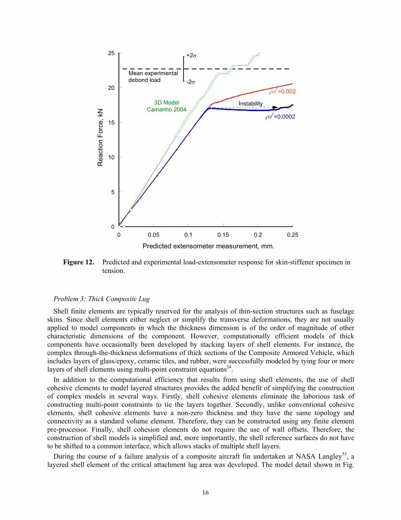
The predicted load-extensometer response for two values of viscoelastic regularization are shown in Fig. 12. The initiation of delamination predicted using a viscoelastic regularization factor of

410.2/ −⋅=Ftρ is 17.2 kN, which is 24% below the mean debond load measured by Cvitkovich28 (22.7 kN). The unstable nature of delamination propagation can be deduced from the reduction of the applied load during the propagation of the delamination. The predicted delamination initiation load using

310.2/ −⋅=Ftρ is 17.5 kN. However, delamination propagation is stabilized by the use of a larger amount of regularization, as can be observed in Fig. 12. The advantage of using a higher amount of regularization is that the solution is obtained much faster than with a lesser amount of regularization: the model with a regularization factor of 410.2 −⋅ took 6 minutes of CPU time on a 3.20GHz Xeon-based PC, while the model with a factor of 310.2 −⋅ took less than 3 minutes.

The previously published results of a 3D model are also shown in Fig. 12. The slope of the force-extensometer curves for the 3D and shell models are different because nodal displacements were used to calculate the extensometer measurement. For the 3D model, the nodes are located on the surface of the laminates, while for the shell models, the nodes are located on the reference surfaces. It can be observed that the 3D model predicts a more accurate debond load of 21.9 kN, which is probably a result of the higher fidelity of the flange tip region in the 3D model.

16

0

5

10

15

20

25

0 0.05 0.1 0.15 0.2 0.25

Rea

ctio

n Fo

rce,

kN

Predicted extensometer measurement, mm.

Instability

ρ/tF=0.002

ρ/tF=0.0002

Mean experimentaldebond load

3D ModelCamanho 2004

+2σ

-2σ

Figure 12. Predicted and experimental load-extensometer response for skin-stiffener specimen in tension.

Problem 3: Thick Composite Lug

Shell finite elements are typically reserved for the analysis of thin-section structures such as fuselage skins. Since shell elements either neglect or simplify the transverse deformations, they are not usually applied to model components in which the thickness dimension is of the order of magnitude of other characteristic dimensions of the component. However, computationally efficient models of thick components have occasionally been developed by stacking layers of shell elements. For instance, the complex through-the-thickness deformations of thick sections of the Composite Armored Vehicle, which includes layers of glass/epoxy, ceramic tiles, and rubber, were successfully modeled by tying four or more layers of shell elements using multi-point constraint equations24.

In addition to the computational efficiency that results from using shell elements, the use of shell cohesive elements to model layered structures provides the added benefit of simplifying the construction of complex models in several ways. Firstly, shell cohesive elements eliminate the laborious task of constructing multi-point constraints to tie the layers together. Secondly, unlike conventional cohesive elements, shell cohesive elements have a non-zero thickness and they have the same topology and connectivity as a standard volume element. Therefore, they can be constructed using any finite element pre-processor. Finally, shell cohesion elements do not require the use of wall offsets. Therefore, the construction of shell models is simplified and, more importantly, the shell reference surfaces do not have to be shifted to a common interface, which allows stacks of multiple shell layers.

During the course of a failure analysis of a composite aircraft fin undertaken at NASA Langley33, a layered shell element of the critical attachment lug area was developed. The model detail shown in Fig.

17

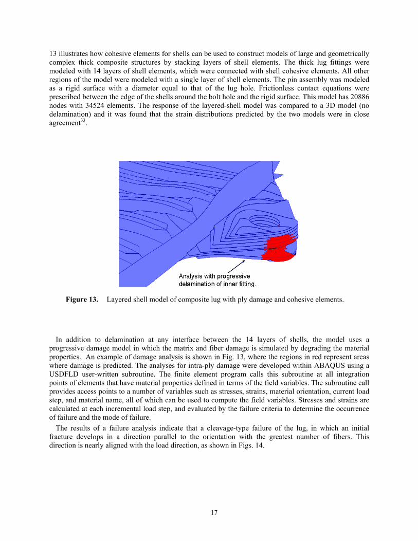
13 illustrates how cohesive elements for shells can be used to construct models of large and geometrically complex thick composite structures by stacking layers of shell elements. The thick lug fittings were modeled with 14 layers of shell elements, which were connected with shell cohesive elements. All other regions of the model were modeled with a single layer of shell elements. The pin assembly was modeled as a rigid surface with a diameter equal to that of the lug hole. Frictionless contact equations were prescribed between the edge of the shells around the bolt hole and the rigid surface. This model has 20886 nodes with 34524 elements. The response of the layered-shell model was compared to a 3D model (no delamination) and it was found that the strain distributions predicted by the two models were in close agreement33.

Figure 13. Layered shell model of composite lug with ply damage and cohesive elements.

In addition to delamination at any interface between the 14 layers of shells, the model uses a progressive damage model in which the matrix and fiber damage is simulated by degrading the material properties. An example of damage analysis is shown in Fig. 13, where the regions in red represent areas where damage is predicted. The analyses for intra-ply damage were developed within ABAQUS using a USDFLD user-written subroutine. The finite element program calls this subroutine at all integration points of elements that have material properties defined in terms of the field variables. The subroutine call provides access points to a number of variables such as stresses, strains, material orientation, current load step, and material name, all of which can be used to compute the field variables. Stresses and strains are calculated at each incremental load step, and evaluated by the failure criteria to determine the occurrence of failure and the mode of failure.

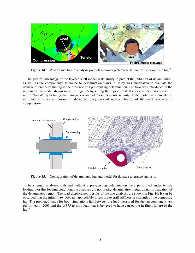
The results of a failure analysis indicate that a cleavage-type failure of the lug, in which an initial fracture develops in a direction parallel to the orientation with the greatest number of fibers. This direction is nearly aligned with the load direction, as shown in Figs. 14.

18

ε22Load

TensionCompression

LoadLoad

12

0°

Failure mode: cleavage

LoadLoad

12

LoadLoad

12

0°

Failure mode: cleavage

Figure 14. Progressive failure analysis predicts a two-step cleavage failure of the composite lug33.

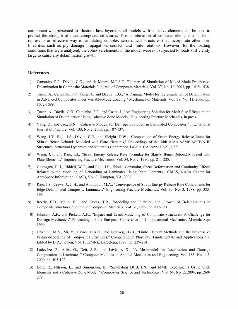
The greatest advantage of the layered shell model is its ability to predict the initiation of delamination, as well as the component’s tolerance to delamination flaws. A study was undertaken to evaluate the damage tolerance of the lug in the presence of a pre-existing delamination. The flaw was introduced in the regions of the model shown in red in Figs. 15 by setting the region of shell cohesive elements shown in red to “failed” by defining the damage variable of these elements as unity. Failed cohesive elements do not have stiffness in tension or shear, but they prevent interpenetration of the crack surfaces in compression.

Figure 15. Configuration of delaminated lug and model for damage tolerance analysis.

The strength analyses with and without a pre-existing delamination were performed under tensile loading. For this loading condition, the analyses did not predict delamination initiation nor propagation of the delaminated region. The load-displacement results of the two analyses are shown in Fig. 16. It can be observed that the initial flaw does not appreciably affect the overall stiffness or strength of the composite lug. The predicted loads for both simulations fall between the load measured for the subcomponent test performed in 2003 and the W375 tension load that is believed to have caused the in-flight failure of the lug33.

19

0

200

400

600

800

1000

1200

0 0.5 1 1.5 2 2.5 3 3.5 4

Rea

ctio

n Fo

rce,

kN

Pin displacement, mm.

w/ initial delaminationno delamination

Subcomponent test, 2003

Design Limit Load

W375 load at failure

Figure 16. Predicted lug strength with and without initial flaw.

Concluding Remarks

The formulation of a cohesive element for shell analysis that can be used to simulate the initiation and growth of delaminations between stacked, non-coincident layers of shell elements was presented. The procedure to construct the element accounts for the thickness offset by applying the kinematic relations of shell deformation to transform the stiffness and internal force of a zero-thickness cohesive element such that interfacial continuity between shell layers is enforced. The internal load vector and the stiffness matrix of a cohesive element connecting shells can be calculated in a very simple way by means of a transformation matrix, independently of the cohesive constitutive models.

Stacks of shell elements can be used to create effective models that predict the inplane and delamination failure modes of thick components. The formulation allows the use of multiple layers of shells through the thickness and it does not require offsetting nodes to a common reference surface. In addition, shell cohesive elements have the same topology as three-dimensional elements so they can be generated using any finite element pre-processor while zero-thickness cohesive elements for three-dimensional elements cannot be generated with most pre-processors.

Using representative examples of increasing structural complexity, it was shown that the proposed cohesive element for shells can be used to represent the propagation of a pre-existing delamination, as well as the onset and propagation of delamination in components that do not contain pre-existing cracks. The analysis of a 50% mode-mix MMB test indicates that the initiation and propagation of delamination under mixed mode can be predicted accurately. It was found that the convergence difficulties that are typical of cohesive laws can be mitigated with the use of viscoelastic regularization or by reducing the interfacial strength to enlarge the process zone. The analysis results of a two-layer model of a skin-stiffener debond indicate that such a simplified model can produce results that may be sufficiently accurate for design and down-select analyses. For better predictive accuracy, models in which the flange taper is represented more accurately would be required. Finally, the analysis results of a large fin lug

20

component was presented to illustrate how layered shell models with cohesive elements can be used to predict the strength of thick composite structures. This combination of cohesive elements and shells represents an effective way of simulating complex aeronautical structures that incorporate other non-linearities such as ply damage propagation, contact, and finite rotations. However, for the loading conditions that were analyzed, the cohesive elements in the model were not subjected to loads sufficiently large to cause any delamination growth.

References

1) Camanho, P.P., Dávila, C.G., and de Moura, M.F.S.F., "Numerical Simulation of Mixed-Mode Progressive Delamination in Composite Materials," Journal of Composite Materials, Vol. 37, No. 16, 2003, pp. 1415-1438.

2) Turon, A., Camanho, P.P., Costa, J., and Davila, C.G., "A Damage Model for the Simulation of Delamination in Advanced Composites under Variable-Mode Loading," Mechanics of Materials, Vol. 38, No. 11, 2006, pp. 1072-1089.

3) Turon, A., Dávila, C.G., Camanho, P.P., and Costa, J., "An Engineering Solution for Mesh Size Effects in the Simulation of Delamination Using Cohesive Zone Models," Engineering Fracture Mechanics, in press.

4) Yang, Q., and Cox, B.N., "Cohesive Models for Damage Evolution in Laminated Composites," International Journal of Fracture, Vol. 133, No. 2, 2005, pp. 107-137.

5) Wang, J.T., Raju, I.S., Dávila, C.G., and Sleight, D.W., "Computation of Strain Energy Release Rates for Skin-Stiffener Debonds Modeled with Plate Elements," Proceedings of the 34th AIAA/ASME/ASCE/AHS Structures, Structural Dynamics and Materials Conference, LaJolla, CA, April 19-21, 1993.

6) Wang, J.T., and Raju, I.S., "Strain Energy Release Rate Formulae for Skin-Stiffener Debond Modeled with Plate Elements," Engineering Fracture Mechanics, Vol. 54, No. 2, 1996, pp. 211-228.

7) Glaessgen, E.H., Riddell, W.T., and Raju, I.S., "Nodal Constraint, Shear Deformation and Continuity Effects Related to the Modeling of Debonding of Laminates Using Plate Elements," CMES, NASA Center for AeroSpace Information (CASI), Vol. 3, Hampton, VA, 2002.

8) Raju, I.S., Crews, J., J. H., and Aminpour, M.A., "Convergence of Strain Energy Release Rate Components for Edge-Delaminated Composite Laminates," Engineering Fracture Mechanics, Vol. 30, No. 3, 1988, pp. 383-396.

9) Reedy, E.D., Mello, F.J., and Guess, T.R., "Modeling the Initiation and Growth of Delaminations in Composite Structures," Journal of Composite Materials, Vol. 31, 1997, pp. 812-831.

10) Johnson, A.F., and Pickett, A.K., "Impact and Crash Modelling of Composite Structures: A Challenge for Damage Mechanics," Proceedings of the European Conference on Computational Mechanics, Munich, Sept 1999.

11) Crisfield, M.A., Mi, Y., Davies, G.A.O., and Hellweg, H.-B., "Finite Element Methods and the Progressive Failure-Modelling of Composites Structures," Computational Plasticity: Fundamentals and Applications '97, Edited by D.R.J. Owen, Vol. 1, CIMNE, Barcelona, 1997, pp. 239-254.

12) Ladevèze, P., Allix, O., Deü, J.-F., and Lévêque, D., "A Mesomodel for Localisation and Damage Computation in Laminates," Computer Methods in Applied Mechanics and Engineering, Vol. 183, No. 1-2, 2000, pp. 105-122.

13) Borg, R., Nilsson, L., and Simonsson, K., "Simulating DCB, ENF and MMB Experiments Using Shell Elements and a Cohesive Zone Model," Composites Science and Technology, Vol. 64, No. 2, 2004, pp. 269-278.

21

14) Bruno, D., Greco, F., and Lonetti, P., "Computation of Energy Release Rate and Mode Separation in Delaminated Composite Plates by Using Plate and Interface Variables," Mechanics of Advanced Materials and Structures, Vol. 12, No. 4, 2005, pp. 285-304.

15) Jin, Z.H., and Sun, C.T., "Cohesive Zone Modeling of Interface Fracture in Elastic Bi-Materials," Engineering Fracture Mechanics, Vol. 72, No. 12, 2005, pp. 1805-1817.

16) Tvergaard, V., "Influence of Plasticity on Interface Toughness in a Layered Solid with Residual Stresses," International Journal of Solids and Structures, Vol. 40, No. 21, 2003, pp. 5769-5779.

17) Tvergaard, V., "Predictions of Mixed Mode Interface Crack Growth Using a Cohesive Zone Model for Ductile Fracture," Journal of the Mechanics and Physics of Solids, Vol. 52, No. 4, 2004, pp. 925-940.

18) Zhang, W., and Deng, X., "Asymptotic Fields around an Interfacial Crack with a Cohesive Zone Ahead of the Crack Tip," International Journal of Solids and Structures, Vol. 43, No. 10, 2006, pp. 2989-3005.

19) Camanho, P.P., Dávila, C.G., and Ambur, D.R., "Numerical Simulation of Delamination Growth in Composite Materials," NASA/TP-2001-211041, Hampton, VA, August 2001.

20) Benzeggagh, M.L., and Kenane, M., "Measurement of Mixed-Mode Delamination Fracture Toughness of Unidirectional Glass/Epoxy Composites with Mixed-Mode Bending Apparatus," Composites Science and Technology, Vol. 56, No. 4, 1996, pp. 439-449.

21) Turon, A., "Simulation of Delamination in Composites under Quasi-Static and Fatigue Loading Using Cohesive Zone Models," PhD Dissertation, Dept. d'Enginyeria Mecànica i de la Construcció Industrial, Universitat de Girona, Girona, Spain, 2006.

22) ABAQUS 6.6 User's Manual, ABAQUS Inc., Providence, RI, USA, 2006.

23) Dávila, C.G., "Solid-to-Shell Transition Elements for the Computation of Interlaminar Stresses," Computing Systems in Engineering, Vol. 5, 1994, pp. 193-202.

24) Dávila, C.G., and Chen, T.-K., "Advanced Modeling Strategies for the Analysis of Tile-Reinforced Composite Armor," Applied Composite Materials, Vol. 7, No. 1, 2000, pp. 51-68.

25) Reeder, J.R., "Load-Displacement Relations for DCB, ENF, and MMB AS4/Peek Test Specimens," Private Communication, 2002.

26) Reeder, J.R., Demarco, K., and Whitley, K.S., "The Use of Doubler Reinforcement in Delamination Toughness Testing," Composites Part A: Applied Science and Manufacturing, Vol. 35, No. 11, 2004, pp. 1337-1344.

27) Minguet, P.J., Fedro, M.J., O'Brien, T.K., Martin, R.H., and Ilcewicz, L.B., "Development of a Structural Test Simulating Pressure Pillowing Effects in Bonded Skin/Stringer/Frame Configuration," Proceedings of the Fourth NASA/DoD Advanced Composite Technology Conference, Salt Lake City, Utah, June 7-11, 1993.

28) Cvitkovich, M.K., Krueger, R., O'Brien, T.K., and Minguet, P.J., "Debonding in Composite Skin/Stringer Configurations under Multi-Axial Loading," Proceedings of the American Society for Composites - 13th Technical Conference on Composite Materials, Baltimore, MD, September 21-23, 1998, pp. 1014-1048.

29) Reeder, J.R., "3D Mixed-Mode Delamination Fracture Criteria–an Experimentalist’s Perspective," Proceedings of the 21st Annual Technical Conference of the American Society for Composites, Dearborn, MI, September 17-20, 2006.

30) Camanho, P.P., Dávila, C.G., and Pinho, S.T., "Fracture Analysis of Composite Co-Cured Structural Joints Using Decohesion Elements," Fatigue & Fracture of Engineering Materials & Structures, Vol. 27, No. 9, 2004, pp. 745-757.

22

31) Krueger, R., París, I.L., O'Brien, T.K., and Minguet, P.J., "Fatigue Life Methodology for Bonded Composite Skin/Stringer Configurations," NASA/TM-2001-210842, Hampton, April 2001.

32) Schellekens, J.C.J., and de Borst, R., "On the Numerical Integration of Interface Elements," International Journal for Numerical Methods in Engineering, Vol. 36, 1993, pp. 43-66.

33) Raju, I.S., Glaessgen, E.H., Mason, B.H., Krishnamurthy, T., and Dávila, C.G., "NASA Structural Analysis Report on the American Airlines Flight 587 Accident - Local Analysis of the Right Rear Lug," Proceedings of the 46th AIAA/ASME/ASCE/AHS/ASC Structures, Structural Dynamics and Materials Conference, Austin, TX, April 18-20, 2005.

REPORT DOCUMENTATION PAGE Form ApprovedOMB No. 0704-0188

2. REPORT TYPE Technical Publication

4. TITLE AND SUBTITLECohesive Elements for Shells

5a. CONTRACT NUMBER

6. AUTHOR(S)

Dávila, Carlos G.; Camanho, Pedro P.; and Turon, Albert

7. PERFORMING ORGANIZATION NAME(S) AND ADDRESS(ES)NASA Langley Research CenterHampton, VA 23681-2199

9. SPONSORING/MONITORING AGENCY NAME(S) AND ADDRESS(ES)National Aeronautics and Space AdministrationWashington, DC 20546-0001

8. PERFORMING ORGANIZATION REPORT NUMBER

L-19341

10. SPONSOR/MONITOR'S ACRONYM(S)

NASA

13. SUPPLEMENTARY NOTESAn electronic version can be found at http://ntrs.nasa.gov

12. DISTRIBUTION/AVAILABILITY STATEMENTUnclassified - UnlimitedSubject Category 39Availability: NASA CASI (301) 621-0390

19a. NAME OF RESPONSIBLE PERSON

STI Help Desk (email: help@sti.nasa.gov)

14. ABSTRACT

A cohesive element for shell analysis is presented. The element can be used to simulate the initiation and growth of delaminations between stacked, non-coincident layers of shell elements. The procedure to construct the element accounts for the thickness offset by applying the kinematic relations of shell deformation to transform the stiffness and internal force of a zero-thickness cohesive element such that interfacial continuity between the layers is enforced. The procedure is demonstrated by simulating the response and failure of the Mixed Mode Bending test and a skin-stiffener debond specimen. In addition, it is shown that stacks of shell elements can be used to create effective models to predict the inplane and delamination failure modes of thick components. The results indicate that simple shell models can retain many of the necessary predictive attributes of much more complex 3D models while providing the computational efficiency that is necessary for design.

15. SUBJECT TERMSCohesive elements; Damage tolerance; Delamination growth; Finite elements

18. NUMBER OF PAGES

2719b. TELEPHONE NUMBER (Include area code)

(301) 621-0390

a. REPORT

U

c. THIS PAGE

U

b. ABSTRACT

U

17. LIMITATION OF ABSTRACT

UU

Prescribed by ANSI Std. Z39.18Standard Form 298 (Rev. 8-98)

3. DATES COVERED (From - To)

5b. GRANT NUMBER

5c. PROGRAM ELEMENT NUMBER

5d. PROJECT NUMBER

5e. TASK NUMBER

5f. WORK UNIT NUMBER

732759.07.09

11. SPONSOR/MONITOR'S REPORT NUMBER(S)

NASA/TP-2007-214869

16. SECURITY CLASSIFICATION OF:

The public reporting burden for this collection of information is estimated to average 1 hour per response, including the time for reviewing instructions, searching existing data sources, gathering and maintaining the data needed, and completing and reviewing the collection of information. Send comments regarding this burden estimate or any other aspect of this collection of information, including suggestions for reducing this burden, to Department of Defense, Washington Headquarters Services, Directorate for Information Operations and Reports (0704-0188), 1215 Jefferson Davis Highway, Suite 1204, Arlington, VA 22202-4302. Respondents should be aware that notwithstanding any other provision of law, no person shall be subject to any penalty for failing to comply with a collection of information if it does not display a currently valid OMB control number.PLEASE DO NOT RETURN YOUR FORM TO THE ABOVE ADDRESS.

1. REPORT DATE (DD-MM-YYYY)04 - 200701-