NASA TECHNICAL NOTE NASA TN 0-7286

*o a0 cv

z c

A FINITE ELEMENT FOR THERMAL STRESS ANALYSIS OF SHELLS OF REVOLUTION

by Howurd M. Adelman, Hdrold C. Lester, dnd James L. Rogers, Jr.

Langley Reseurch Center Hampton, Vu. 23665

N A T I O N A L AERONAUTICS A N D SPACE A D M I N I S T R A T I O N W A S H I N G T O N , D. C. DECEMBER 1973

https://ntrs.nasa.gov/search.jsp?R=19740004438 2018-11-21T23:18:47+00:00Z

1. Repon No. 2. Government Accession No.

NASA TN D-7286 4. Title and Subtitle

A FINITE ELEMENT FOR THERMAL STRESS ANALYSIS OF SHELLS OF REVOLUTION

19. Security Classif. (of this report) 20. Security Classif. (of this page)

Unclassified Unclassified

7. Authods) Howard M. Adelman, Harold C. Lester, and James L. Rogers, Jr.

9. Performing Organization Name and Address

NASA Langley Research Center Hampton, Va. 23665

21. No. of Pages

57

2. Sponsoring Agency Name and Address

National Aeronautics and Space Administration Washington, D.C. 20546

3. Recipient's Catalog No.

5. Report Date December 1973

6. Performing Organization Code

8. Performing Organization Report No.

L-8679 10. Work Unit No.

501 -22-01-01

11. Contract or Grant No.

13. Type of Report and Period Covered

Technical Note 14. Sponsoring Agency Code

5. Supplementary Notes

6. Abstract

This report describes a new finite element for performing detailed thermal s t r e s s analysis of thin orthotropic shells of revolution, The element provides for temperature loadings which may vary over the surface of the shell as well as through the thickness. In a number of sample calculations, results from the present method a r e compared with ana- lytical solutions as well as with independent numerical analyses. Such calculations a r e carried out for two cylinders, a conical frustum, a truncated hemisphere, and an annular plate. Generally, the agreement between the present solution and the other solutions is excellent.

17. Key Words (Suggested by Author(s1)

Shell of revolution Finite-element method Thermal s t r e s s

~~~ ~ ~

18. Distribution Statement

Unclassified - Unlimited

22. Price'

Domestic 3 50 Foreign: $6:00

A FINITE ELEMENT FOR THERMAL STRESS ANALYSIS

OF SHELLS O F REVOLUTION

By Howard M. Adelman, Harold C. Lester, and James L. Rogers, Jr. Langley Research Center

SUMMARY

This report describes a new axisymmetric finite element for calculating static thermal s t resses in general orthotropic thin shells of revolution. The element is geo- metrically exact and the thermal loading conditions allow for variations over the shell surface as well as through the shell thickness.

The elem-ent is utilized in a number of sample calculations on a variety of shell shapes and loading conditions. Among the shells analyzed a r e two cylinders, a conical frustum, a truncated hemisphere, and an annular plate. Results from the present method a r e compared with either exact solutions which a re developed in the report or with resul ts from other methods based on finite differences. The results predicted by the present method were found to be in excellent agreement with the exact solutions and the finite- difference solutions.

INTRODUCTION

The capability to predict reliably the static s t r e s s of structural components sub- jected to thermal loads has become an urgent need for structural designers and analysts. Of particular interest a r e aerospace vehicles undergoing aerodynamic heating during atmospheric entry and aircraft structures heated by impinging jet engine exhaust. In many instances the aerospace vehicles of interest are thin shells of revolution. Closed-form analytical solutions to thermal stress problems for this c lass of structure have been obtained only for limited geometries and loading conditions (refs. 1 to 3). era l geometries and loadings it is usually necessary to resor t to approximate methods such as finite differences (refs. 4 to 6), numerical integration (ref. 7), or the finite- element method (ref. 8). Finite-difference methods and numerical integration techniques have been used with a good deal of success for thermal s t r e s s analysis of shells of revo- lution with a high degree of generality in the thermal loadings.

For more gen-

The finite-element method has developed into the primary analysis tool for complex structures such as complete aerospace vehicles. Large comprehensive finite-element programs such as NASTRAN (ref. 8) have a variety of finite elements available to the user for modeling almost any conceivable configuration. However the elements themselves, especially the shell of revolution elements, are quite primitive both with regard to their shape and the generality of thermal loads that can be applied, particularly when compared

with the generality available in the previously mentioned approaches. It appears then that the finite-element method can be made more useful with regard to thermal stress analysis by introducing new and/or improved elements which have the kind of generality that is available in the finite-difference and numerical integration approaches. Accordingly, an improved axisymmetric finite element for thermal stress analysis of shells of revolution has been developed.

The purpose of the present report is to describe and evaluate the new finite element. The finite element is geometrically exact, a concept previously utilized for analysis of free vibrations (refs. 9 and 10) and of temperature distributions in shells of revolution (ref. 11).

The report contains a description of the mathematical development of governing matrices for the element and describes a number of sample calculations carr ied out to verify the accuracy and versatility of the element. These calculations are performed for cylinders under two different loading conditions, a conical frustum, a truncated hemisphere, and an annular plate. Wherever possible analytical solutions (some derived herein) are used for checking results. There a r e three appendixes to this report. Appendix A con- tains a summary of the basic equations governing the finite element; appendix B contains the derivation of the thermal stress in an annular plate under a quadratically varying temperature; and appendix C contains a method for obtaining exact modal solutions for thermal s t resses in freely supported cylinders.

a

b

cn = (1'

'66

SYMBOLS

inner radius of annular plate (appendix B)

coefficients in polynomial displacement function for normal displacement w

outer radius of annular plate (appendix B)

coefficients in polynomial displacement function for meridional displacement u

(n = 0)

(n f o ,

membrane stiffnesses

in-plane shear stiffness

2

el’ e2

e12

t ,t t el, 2’ e12

coefficients in polynomial displacement function for circumfer- e ntial displace me nt v

flexural stiff ne sse s

torsional st iff ness

Young’s modulus for meridional and circumferential directions, respectively

middle-surface strains in meridional and circumferential directiens, resPectis.ely

middle-surface shear strain

total strains

thermal force column matrix for complete shell

element thermal force column matrix

thermal force column matrix (see eqs. (12) and (13))

modal force column matrix (eq. (29))

shear modulus

shell thickness

identity matrix

K number of finite elements used to represent shell

stiffnesses representing interaction between in-plane and out-of- K1l’ K12’ K22’ K66 plane strains

3

L meridional length of shell

Mtl’ Mt2

M1’ M12

m

N

thermal moment resultants in meridional and circumferential directions, respectively

moment resultants in meridional and circumferential directions and twisting moment, respectively

meridional wave number for freely supported cylinder

order of stiffness matrix and force vector after edge constraints have been applied

thermal forces in meridional and circumferential directions, respectively

circumferential wave number

principal radii of curvature of shell

radius of shell measured in plane normal to shell axis

shell stiffness matrix

meridional coordinate

temperature

temperatures at inner and outer fiber of shell, respectively

matrix relating coefficients of assumed displacement shapes to degrees of freedom on edges of element

maximum value of temperature

stress resultants in meridional and circumferential directions, respective ly

T12

U

U

V

V

W

[XI

X

{ Y )

z

al’ a2

P

‘k

e

K1’ K2

12

W

shear s t r e s s resultant

total potential energy

meridional component of middle- surface displacement

strain energy

circumferential component of middle-surface displacement

normal component of middle- surface displacement

matrix which describes assumed form of variables appearing in strain energy

meridional coordinate measured within single element

column matrix containing unknown displacements, rotations, and derivatives thereof

coordinate in direction normal to shell surface

coefficients of linear thermal expansion in meridional and cir- cumferential directions, respectively

U rotation of shell generator, w’ - -

R1

length of kth finite element

circumferential coordinate

changes in curvature in meridional and circumferential direc- tions, respectively

twist of middle surface

diagonal matrix of eigenvalues of stiffness matrix

A

'm

eigenvalue of stiffness matrix

mode parameter for freely supported cylinder, mn/L (appendix C)

Poisson's ratio for meridional and circumferential directions, respectively

column matrix whose elements a r e displacements and rotations and their derivatives at ends of kth element

mass density

meridional and circumferential s t resses , respectively

shear st re ss

modal matrix for stiffness matrix

potential energy associated with thermal loading

number of element or number of first edge of element

number of second edge of element

P

u 1 9 "2

O12

[+I

n

Subscripts:

k

k+ 1

Superscript :

n circumferential harmonic number

Primes denote differentiation with respect to s or x; T denotes transpose of a matrix.

ANALYSIS METHOD

In this section of the report, the governing matrix equations are derived. The procedure follows very closely the development in reference 9. The strain energy for a thin orthotropic shell of revolution is derived in te rms of the three components of dis- placement of the shell middle surface and in t e rms of the shell temperature. A finite-

6

element representation of the shell is introduced in which the shell is represented by congruent sl ices of the shell and the displacement components a r e approximated by polynomials. The potential energy is minimized to obtain the governing matrix equations which involve two main contributions: the stiffness matrix and the thermal load vector. The stiffness matrix is identical to that presented in reference 10. The present develop- ment derives the thermal load vector.

Derivation of Governing Equations

Pertinent geometrical quantities a r e defined in figure 1. The components of dis-

placement in the meridional, circumferential, and normal directions a re denoted by u, v, and w, respectively. A point in the shell is defined by the meridional, circumferential, and normal coordinates s, 0 , and z, respectively. The two principal radii of curva- ture of the siieii iiiiddk surface a r e El ana R2 and the distance from the axis of the shell to a point on the middle surface is r.

The s t ress-s t ra in relations for a linear orthotropic material including effects of temperature as given in reference 1 2 a re

t O12 = Ge12 I

where the subscripts 1 and 2 refer to the meridional and circumferential directions, respectively, and plE2 = p2E1.

The s t ra in energy of the shell modified for a two-dimensional orthotropic material is conveniently written according to reference 13 as

t t U = 1 J j J Ele i + u2e2 + m12e12 2 s e z

It is assumed that lines originally normal to the middle surface remain straight, unex- tended, and normal after deformation. The total strains then have the following variation through the shell thickness:

7

Substituting equations (3 ) into equation (2), rearranging, and discarding a constant involv- ing the known temperature yield:

I

u = v - n

where

v = 'JJ (Cllel 2 + 2C12ele2 + C22e2 2 + C66e:2 )r do ds 2

(4)

+ AJJ (KllelK1 + K12(~1e2 + x2e1) + K22e2.y2 t K66e12~12)r de ds (5) 2

(Ntlel + MtlKl + Nt2e2 + M t2 K 2 ) r de ds (6)

In equation (5), V is the strain energy of the shell which is utilized in the development of the stiffness matrix in references 9 and 10 and presented in this report for complete- ness. The stiffnesses in equation (5) a r e needed in a later section of the report and are given in table 1. The rest of the present development consists of operating on the thermal potential energy to obtain the thermal load vector.

In equation (6), the quantities Ntl and Nt2 are thermal forces and Mtl and are thermal moments which are defined as follows: Mt2

8

The components of displacement and the temperature a r e assumed to have the following separable forms for each harmonic n:

u(s,e) = u(s) cos ne

v(s,B) = v ( s ) sin n e

w(s,e) = w(s) cos no

T(s,B,z) = T(s,z) cos ne

The s t ra in displacement relations used a r e those of Novozhilov as used in reference 9 and repeated here for completeness:

Middle- surface s t ra ins :

W e; = u' + - *1

9

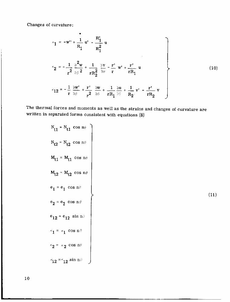
Changes of curvature:

e

1 Ri K1 = -w"+ - u' - - u

R1 RS i r' K 1 2 = - - - + - 1 aw' r' - + - - + - v ' aw 1 au 1 --v

r ae 2 a8 rR1 28 R2. rR2

The thermal forces and moments as well as the s t ra ins and changes of curvature are written in separated forms consistent with equations (8)

N = N~~ cos ne 7 t l

Mtl = Mtl cos n8

Mt2 = q2 cos no

el = e l cos ne

e2 = e2 cos n e

e12 = e12 sin no

K~ = K~ cos n e

~2 = ~2 COS ne

I K~~ = K ~ ~ sin nH

10

where Ntl, Nt2, Mtl, and so forth a r e functions of s only. Substituting equations (9) and (10) along with equations (11) into equation (6) yields

R = C 1 {w, w', w", u, u', v, v')* { f ) d s n

where {f 1 is a 7 X 1 column matrix whose elements a r e given in the following equations:

2 r r n f l = - N +-N t 2 + r t2

R2 t l

R1

f 2 = -r'Mt2

f3 = - rMtl

r r' f - r 'Nt2 -- R'M + - 2 R1

4 - 1 t l

f = rNtl + - Mtl R1

5

r Mt2 f - rNt2 + -

R2 6 -

f7 = 0

The integration with respect to e ,;om 0 to 27r ..as been performed and use was made of the following results:

( n = 0)

( n > 0) cn= 5,"" cos ne de =

11

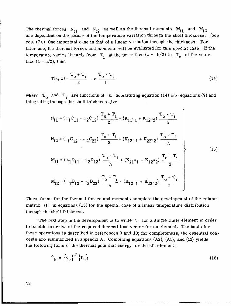
The thermal forces Ntl and Nt2 as well as the thermal moments Mtl and Mt2 are dependenc on the nature of the temperature variation through the shell thickness. eqs. (7).) One important case is that of a linear variation through the thickness. For later use, the thermal forces and moments will be evaluated for this special case. If the temperature varies linearly from Ti at the inner face ( z = -h/2) to To at the outer face ( z = h/2), then

(See

To + Ti To - Ti T(s, Z ) = + z (14) 2 h

where To and Ti are functions of s. Substituting equation (14) into equations (7) and integrating through the shell thickness give

\

To + Ti To - Ti Ntl = (a lCl l + a C 2 12) + (K11"1+ K12Q2)

h

To - Ti To + Ti 2 M t2 = ( a D 1 12 + "zD22) + (K12"l + K22a2)

These forms for the thermal forces and moments complete the development of the column matrix { f } in equations (13) for the special case of a linear temperature distribution through the shell thickness.

The next step in the development is to write R for a single finite element in order to be able to arr ive at the required thermal load vector for an element. The basis for these operations is described in references 9 and 10; for completeness, the essential con- cepts are summarized in appendix A. Combining equations (A2), (A5), and (12) yields the following form of the thermal potential energy for the kth element:

12

~

where {Fk} is the thermal load column matrix for the kth element as given by

Formulation and Solution of Final Equations

A s in reference 10, the following conditions of compatibility are imposed at each element juncture :

wk+ 1

'k+ 1

'k+l

pk+l

UL+ 1

vi+ 1

fi+1 k element

wk+l

'k+l

'k+l

pk+l

u;r+ 1

'k+l

&+ 1 k+l element

Of the seven conditions of compatibility shown in equation (18), only the first four are strictly required to assure that the element converges. The last three conditions a r e imposed in order to improve the convergence characteristics of the element. Specifically, these conditions require continuity of strains and change of curvature at element junctures and evidence of the improved accuracy resulting from this continuity has been presented in reference 12.

Two final observations a r e that the last three conditions are not correct for shells which have a step discontinuity in stiffness at an element juncture and that for problems in which the theoretical s t r e s s distribution has a slope discontinuity, the present element will display a "rounded corner" at the location of the slope discontinuity.

13

The total thermal potential energy is obtained by summing the element contributions; thus,

K

where Ok is given in equation (16). When the summation indicated in equation (19) is carr ied out and u s e is made of equations (17) and (18), the thermal potential energy may be written as

T R = {y) iF)

where

{F 1 thermal load column matrix of order 7(K + 1)

{ Y } column matrix containing the unknown displacements, rotations, and deriva- tives thereof

From reference 9, the s t ra in energy may be written

1 T 2

v = - { y ) [SI @>

where positive semidefinite matrix of order 7(K + 1). The formation of the stiffness matrix has been described in references 9 and 10 and need not be discussed further. The formation of the thermal force column matrix for the complete shell from the element thermal force column matrices is accomplished by overlapping the last seven numbers in each column matrix with the first seven numbers in the adjacent (higher numbered) column matrix. Finally the column matrix {y> is the union of the column matr ices {ek> as defined in equation (A6).

[SI represents the stiffness matrix which is a symmetric positive definite or

The equations governing the behavior of the shell before edge constraints are applied are derived by minimizing the total potential energy. Thus,

s(v - n) = 0 (22)

The minimization in equation (22) is equivalent to the following matrix equation:

[SI@} = {F)

14

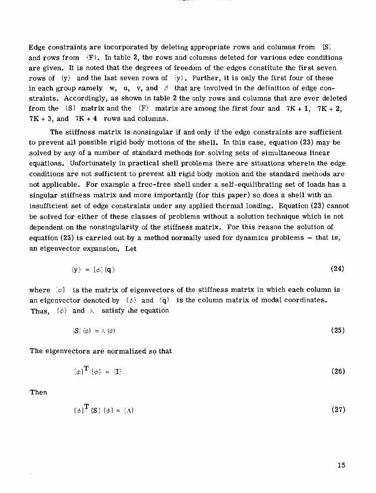
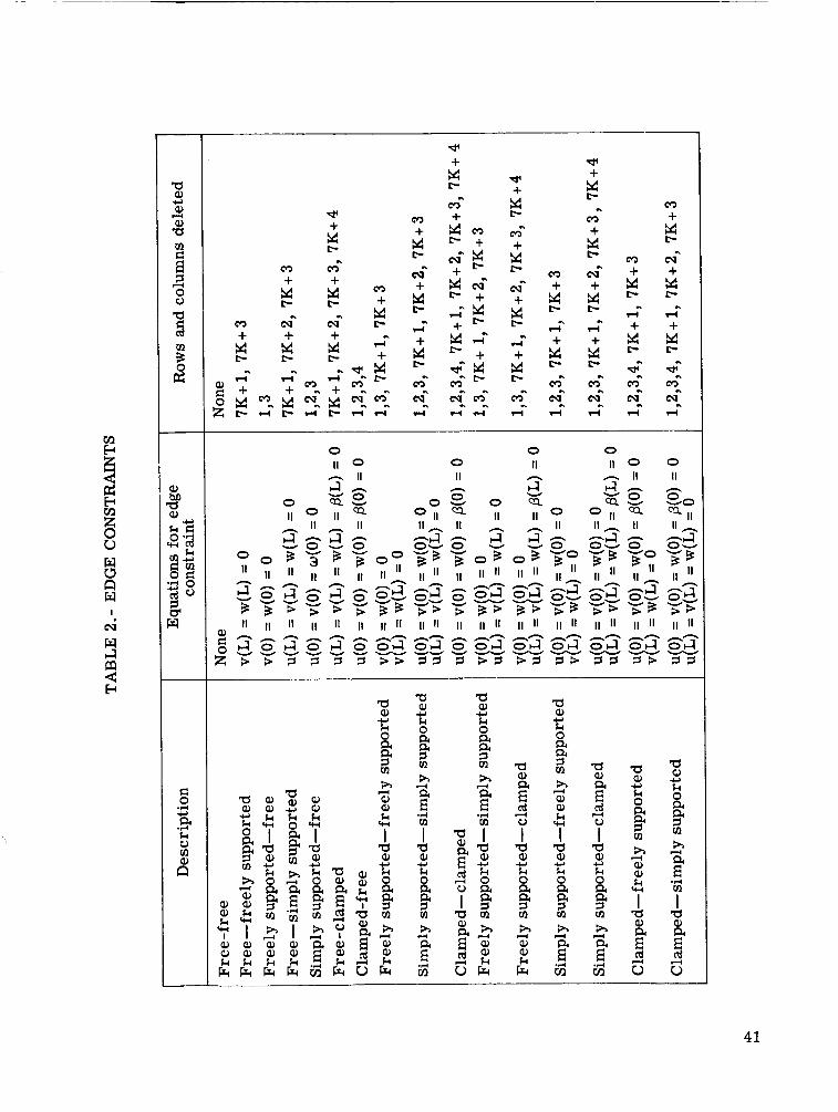
Edge constraints a r e incorporated by deleting appropriate rows and columns from and rows from {F). In table 2, the rows and columns deleted for various edge conditions a r e given. It is noted that the degrees of freedom of the edges constitute the first seven rows of {y) and the last seven rows of {y?. Further, it is only the first four of these in each group namely w, u, v, and P that are involved in the definition of edge con- straints. Accordingly, as shown in table 2 the only rows and columns that a r e ever deleted from the [SI matrix and the IF) matrix a re among the first four and 7K + 1, 7K + 2, 7K + 3, and 7K + 4 rows and columns.

[SI

The stiffness matrix is nonsingular if and only if the edge constraints a r e sufficient to prevent all possible rigid body motions of the shell. In this case, equation (23) may be solved by any of a number of standard methods for solving sets of simultaneous linear equations. Unfortunately in practical shell problems there a r e situations wherein the edge conditions are not sufficient to prevent aii rigid body motion ana t i e standara metnods are not applicable. For example a free-free shell under a self-equilibrating set of loads has a singular stiffness matrix and more importantly (for this paper) so does a shell with an insufficient set of edge constraints under any applied thermal loading. Equation (23) cannot be solved for either of these classes of problems without a solution technique which is not dependent on the nonsingularity of the stiffness matrix. For this reason the solution of equation (23) is carr ied out by a method normally used for dynamics problems - that is, an eigenvector expansion. Let

where [+I an eigenvector denoted by t4) and (q? is the column matrix of modal coordinates. Thus, 141 and A satisfy ihe equation

is the matrix of eigenvectors of the stiffness matrix in which each column is

The eigenvectors a r e normalized so that

Then

15

where

T Substituting equation (24) into equation (23), premultiplying by [+I , and making use of equation (27) give

T where {TI = [+I {F) is the generalized force column matrix in which the ith element of <f> is the component of force that would deform the shell into the shape characterized by the ith eigenvector of [SI. The solution of equation (29) is as follows

Fibi 1

0 q * = { (i = 1, 2, . . ., N) (30)

( A i f 0)

( A i = 0)

The column matrix {y) is then obtained from equation (24).

Displacement and Stress Recovery

The coefficients of the polynomials representing the displacement field are obtained from equation (A5). The displacement components u, v, and w are then obtained by use of the equations:

2 3 4

2 3

2 3

= aO,k + al,kx + a2,kx + a3,kx + a4,kx + a5,kx

= bO,k + bl,kx + b2,kx + b3,kx

v = c O,k+ 'l,l? + '2,l? + '3,kX

16

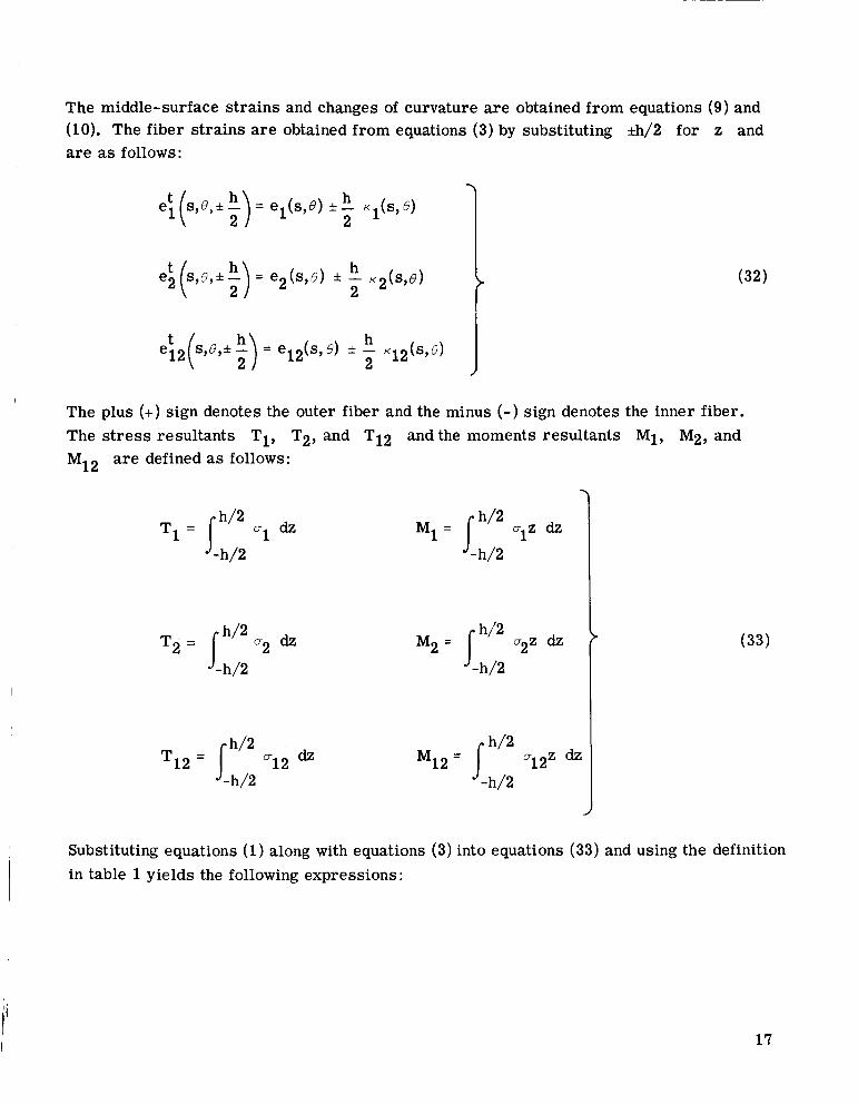
The middle-surface s t ra ins and changes of curvature a r e obtained from equations (9) and (10). The fiber strains are obtained from equations (3) by substituting *h/2 for z and a r e as follows:

The plus (+) sign denotes the outer fiber and the minus (-) sign denotes the inner fiber. The stress resultants TI, T2, and T12 and the moments resultants Mi, M2, and M12 are defined as follows:

J-h/2

J-h/2

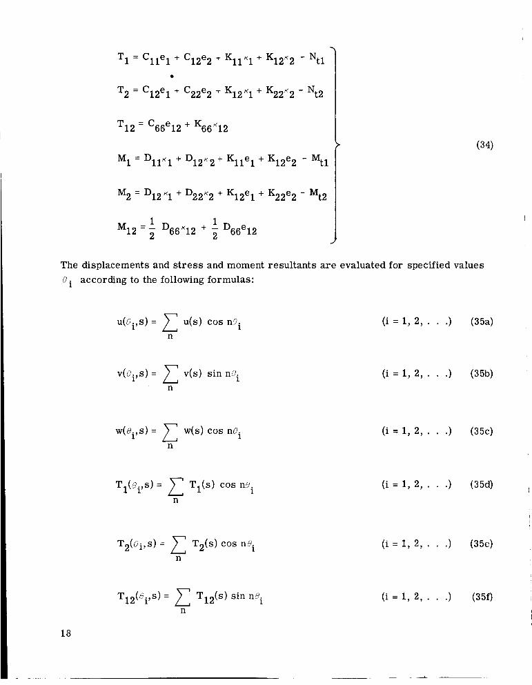
Substituting equations (1) along with equations (3) into equations (33) and using the definition in table 1 yields the following expressions:

17

e

T1 = %le1 + C12e2 + K l l K l + K12K2 - Ntl

T2 = C12el + C22e2 + K12K1 + K22K2 - Nt2

T12= C 66 e 12 + K66~12

M1 = D l l ~ l + D I ~ K ~ + K e + K12e2 - Mtl 11 1

(34)

M2 = D12~1 + D 2 2 ~ 2 + K e + K22e2 - Mt2 12 1

1 1 M12 = D66~12 + - D e 2 66 12 I

The displacements and stress and moment resultants are evaluated for specified values 6 according to the following formulas:

i Tl(ei,s) = T1(s) cos ne n

(i = 1, 2, . . .) (35a)

(i = 1, 2, . . .) (35b)

(i = 1, 2, . . .) (35c)

(i = 1, 2, . . .) (35d)

1 1

(i = 1, 2, . . .) (35e)

(i = 1, 2, . . .) (35f)

18

M2(Bi,s) = M2(s) cos nei n

Ml2(Oi,s) = M12(s) sin nei n

(i = 1, 2, . . .) (35g)

(i = 1, 2, . . .) (35h)

(i = 1, 2, . . .) (3%)

I The range of summation on n is over the number of circlimfermtial harmonics considered.

EVALUATION OF THE ELEMENT

In order to verify the validity and versatility of the new element, sample calculations were performed for a variety of shell geometries and thermal loads. Analytical solutions were available for some of the models. In the following sections a r e presented descrip- tions of the shells, the methods of evaluating numerical results, the finite-element repre- sentations, and detailed evaluations of the results.

,

Description of Shells Analyzed

The geometry of the shells analyzed a re illustrated in figure 2 along with the cor- responding temperature loading functions and the shell material properties. For cylin- ders I and I1 and the truncated hemisphere, the temperature is constant through the shell thickness. the thickness. edge conditions are clamped-clamped. Also, the temperatures a r e axisymmetric except for cylinder 11. A brief description of each shell is given as follows:

For the conical frustum and the annular plate, the temperature var ies through For all shells except cylinder 11, which has freely supported edges, the

I Cylinder I is a cylindrical shell having a temperature distribution with a discontinu- ous slope at the midlength of the cylinder (s/L = 1/2). This discontinuity occurs when the midlength circumference is maintained at a prescribed temperature. The temperature dis- tribution (derived in refs, 3 and 11) illustrates the behavior of the present finite element for a stress distribution having a slope discontinuity.

Cylinder II is a cylindrical shell with a temperature distribution which is constant along the length of the shell but varies around the circumference. This temperature dis- tribution (derived in refs. 3 and 11) results when a generator of the cylinder is maintained at a constant temperature. This example was chosen to illustrate the application of the

19

finite element to a nonaxisymmetric temperature distribution and also to illustrate an application where, because of the freely supported edge conditions, the stiffness matrix is singular.

An orthotropic 30' conical frustum has a temperature distribution which varies quadratically along the shell length and linearly through the thickness. This distribution is an approximation to that in the vicinity of the nose nf a missile undergoing aerodynamic heating (ref. 14). This example illustrates the use of the present element for orthotropic shells, for a nonconstant shell radius, and for an applied thermal bending moment.

A truncated hemisphere having a temperature distribution (derived in ref. 11) cor- responding to a uniform heat flux over the outer surface of the shell was chosen to illus- t ra te a calculation for a shell with a curved generator such that both principal radii of curvature are nonzero.

An annular plate with a temperature varying linearly through the thickness and quadratically from the inner radius to the outer radius illustrates the application of the element when thermal bending moments are applied as the loads and fo r the limiting case of an annular plate.

Method of Evaluation

The evaluation of the element was accomplished by using a computer program to calculate stress and moment resultants and then by comparing the results with other solutions for the same configurations. Check solutions were obtained from the following sources :

For cylinder I, an analytical solution was available from reference 3

For cylinder 11, a converged modal solution was generated based on the procedure I

described in appendix C, and results were obtained for harmonics n = 0 to 4

For the orthotropic conical frustum, check results were available from the finite- difference computer programs of references 5 and 6

For the truncated hemisphere, a solution was available f rom reference 5

For the annular plate, an analytical solution derived in appendix B was utilized I

Detailed comparisons between resul ts with the present method and resul ts from these 4i

sources are presented in a later section.

Finite - E le ment Repre sentat ion

The number and spacing of elements in the shell representations are given in table 3. These representations were arrived at by the following procedure: first, each shell

20

was analyzed with a representation of 10 equally spaced elements and r e s u l t s were com- pared with the appropriate check solution. If satisfactory agreement was obtained (as for cylinder II and the annular plate), no refinement was performed. If the results were not satisfactory, a more refined representation of the shell was made in the vicinity of the edges of the shells where the steepest gradients in the stress distributions are found. The refinements were similar to those done in the modal s t r e s s study of reference 12. The final represectations used to give the results in the present report are those in table 3.

Evaluation and Discussion

Calculated resuits r'i-sm the present finite-element and other analyses are presented in tables 4 to 8 and in figures 3 to 8. In this section, an evaluation of the performance of the element for each set of calculations is presented. Before proceeding to discussions of individual shells, two general observations are made.

(1) For all shells except cylinder XI, results a r e axisymmetric; that is, they corre- spond to n = 0 because of the axisymmetric character of the temperature loads

(2) For all shells except the annular plate, the moment resultants are negligibly small and a r e not presented

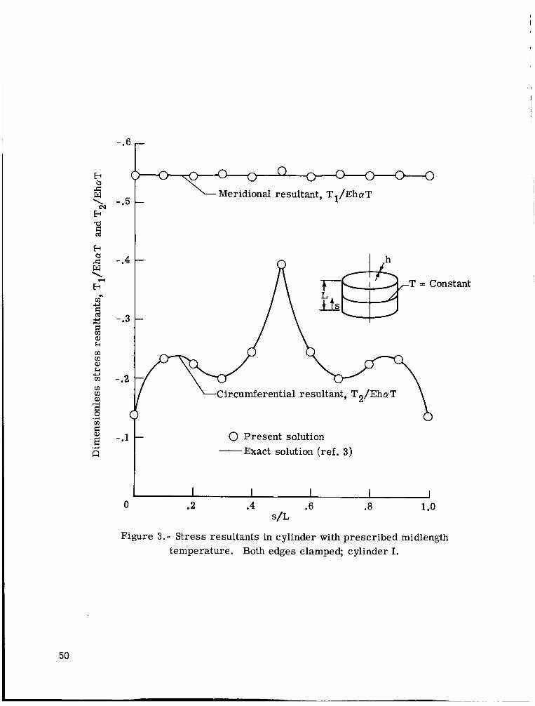
Cylinder I.- Nondimensional meridional and circumferential s t ress resultants pre- dicted by the present method for cylinder I are presented along with analytical resul ts f rom reference 3 in table 4. The s t r e s s resultant distributions a re necessarily symmet r i c about the midlength of the cylinder as a consequence of the symmetry of the load and the edge conditions. The analytical solution for th i s example as given in reference 3 shows a constant meridional s t r e s s resultant TI, whereas the present finite-element solution exhibits a slight oscillation about the constant value. The maximum er ror of 0.6 pe rcen t occurs at the midlength of the cylinder. The comparison for the circumferential stress resultants T2 also shows close agreement, the largest e r r o r being 0.4 percent. In figure 3, the s t ress resultants are plotted with the analytical solution being r e p r e s e n t e d by the solid curves and the present finite-element solution indicated by the c i r c l e s . It is of particular interest to observe that the analytical solution for has a Cusp - that is, a discontinuity in the slope at the cylinder midlength as a result of the discontinuity in the slope of the temperature distribution at that location. Since the displacement field a s s u m e d for the finite element implies continuity in the slope of the s t ress resultants it might be expected that the element would have difficulty converging in the vicinity of such a c u s p . However as indicated in figure 3, no such difficulty was found, and although there is a local rounding of the cusp, this rounding was too negligible to be plotted and had no appreciable effect on the accuracy of the s t r e s s resultant.

T2

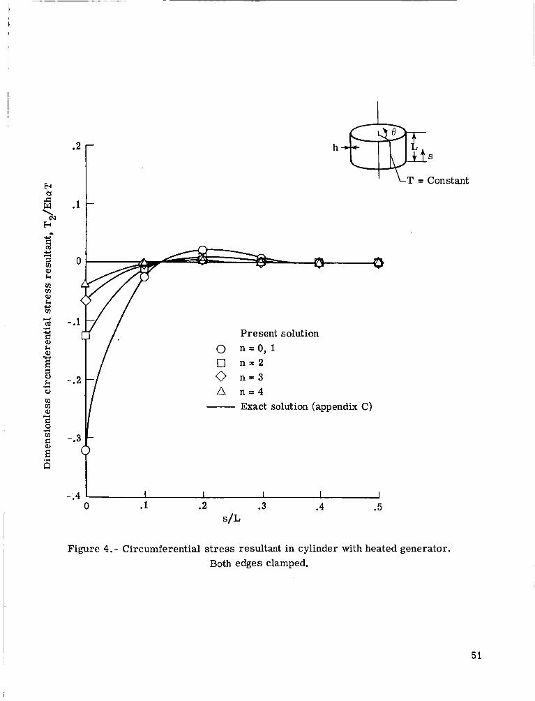
Cylinder II.- Circumferential s t ress resultants T2 for cylinder II f o r values of n

2 1 f rom 0 to 4 are shown in table 5 . In this table, the exact solution was obtained by the modal

Present analysis

SADAOS SALORS (ref. 6) (ref. 5)

22

Smaller end

Larger end

-28.17 -29.44 -28.89

-12.24 -10.82 -12.27

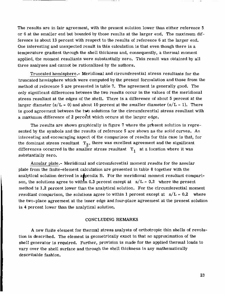
The results a r e in fair agreement, with the present solution lower than either reference 5 or 6 at the smaller end but bounded by those results at the larger end. The maximum dif- ference is about 13 percent with respect to the results of reference 6 at the larger end. One interesting and unexpected result in this calculation is that even though there is a temperature gradient through the shell thickness and, consequently, a thermal moment applied, the moment resultants were substantially zero. This result was obtained by all three analyses and cannot be rationalized by the authors.

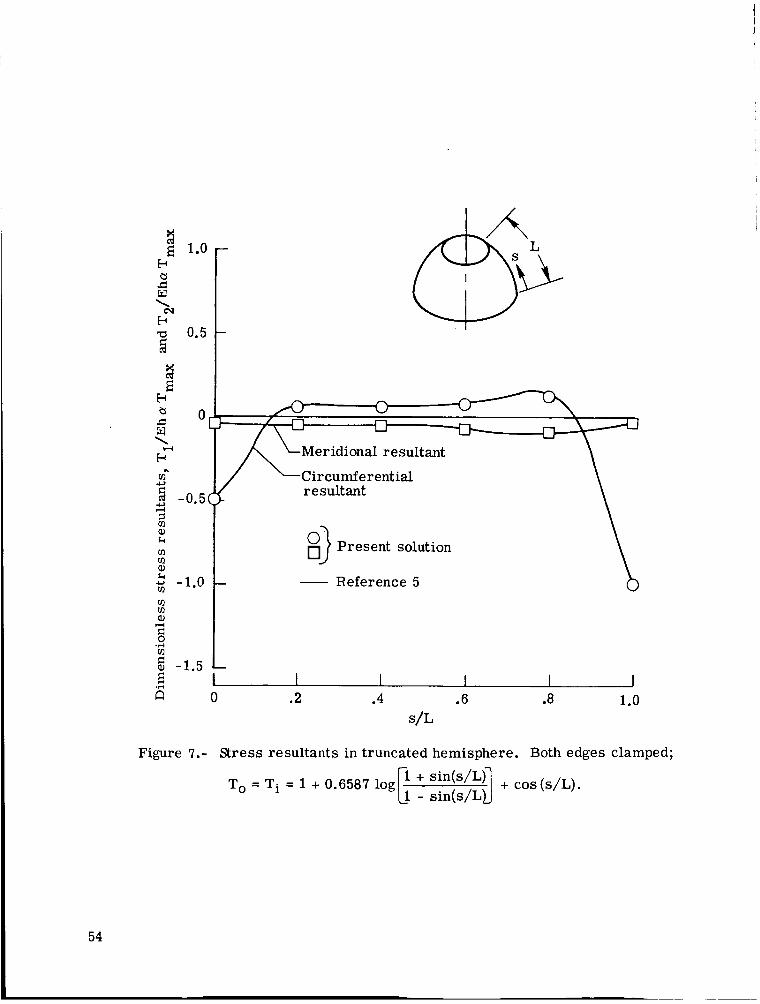
Truncated hemisphere.- Meridional and circumferential s t r e s s resultants for the truncated hemisphere which were computed by the present formulation and those from the method of reference 5 a r e presented in table 7. The agreement is generally good. The only significant differences between the two results occur in the values of the meridional s t r e s s resultant at the edges of the shell. There is a difference of about 5 percent at the larger diameter (s/L = 0) and about 10 percent at the smaller diameter (s/L = 1). There is good agreement between the twb solutions €or the circumferential s t r e s s resultant with a maximum difference of 2 percent which occurs at the larger edge. L

The results a r e shown graphically in figure 7 where the prksent solution is repre- sented by the symbols and the results of reference 5 a r e shown as the solid curves. An iiiLeiebLiiig and encouraging aspect of the comparison of resul ts f o r this case is thzt, f o r the dominant s t r e s s resultant T2 , there w a s excellent agreement and the significant differences occurred in the smaller s t ress resultant at a location where it was substantially zero.

---A ---- -A:-

T1

Annular plate.- Meridional and circumferential moment results for the annular plate from the finite-element calculation a r e presented in table 8 together with the analytical solution derived in a pendix B. For the meridional moment resultant compari-

method is 1.2 percent lower than the analytical solution. For the circumferential moment resultant comparison, the solutions agree t o within 1 percent except at s/L = 0.2 where the two-place agreement at the inner edge and four-place agreement at the present solution is 4 percent lower than the analytical solution.

son, the solutions agree to with f n 0.3 percent except at s/L = 0.2 where the present

CONCLUDING REMARKS

A new finite element for thermal stress analysis of orthotropic thin shells of revolu- tion is described. The element is geometrically exact in that no approximation of the shell generator is required. Further, provision is made for the applied thermal loads to vary over the shell surface and through the shell thickness in any mathematically describable fashion.

23

Sample calculations are carr ied out on a variety of shell models and resul ts f rom the present method are compared either with analytical solutions or with numerical resul ts from independent analyses. Among the shell configurations analyzed are cylinders under two different thermal loading conditions, a conical frustum, a truncated hemisphere, and an annular plate. For these calculations the results from the new finite element generally are in good agreement with the check solutions. The only significant inaccuracies were observed in some stress resultants near the clamped edges of the conical frustum and the hemisphere where the stress gradients were particularly severe and consequently where finite-element analyses usually require significant refinement before convergence is obtained.

The nature of the finite element is such that continuity of s t ra ins and curvatures is maintained at all points along the shell. Consequently in a shell where there is theoreti- cally a slope discontinuity or cusp i n a stress or moment resultant the results predicted by the present method will show a slight local smoothjNg of the cusp but this has no adverse effect on the aecuracy of the results. w

24

Langley Research CentCr, National Aeronautics and Space Administration,

Hampton, Va., June 30, 1973.

APPENDIX A

REPRESENTATION OF A SHELL OF REVOLUTION BY GEOMETRICALLY

EXACT FINITE ELEMENTS

The basic assumptions underlying the finite element and a detailed derivation of the stiffness matrix a r e given in references 9 and 10. The purpose of this appendix is to summarize the concepts, conventions, and equations needed in the development of the thermal load vector for a geometrically exact finite element.

The following notation is used (fig. 9):

K total number of elements used to represent shell

meridional length of kth finite element

coordinate in kth element, measured from center of element so that € k X

A subscript notation is established in which a subscript k, when used with a quantity such as u, v, w, p , R1 or their derivatives, implies that the quantity is evaluated

‘k a t the f i rs t edge of the element x = -2. Similarly, a subscript k+l, when used with

such quantities, implies that they are evaluated at the second edge of the element

‘k x = 2‘ means that the quantity with the subscript is evaluated for the kth element. The displace- ment components o r derivatives thereof within the kth element a r e approximated by poly- nomials as follows (ref. 10):

In all other uses of the subscript k, for example, for matrices and vectors, it

I

25

APPENDIX A

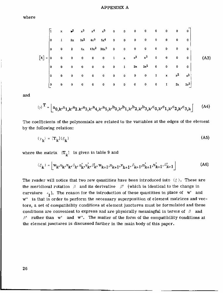
- - 1 x ~ x 3 x 4 x 5 0 0 0 0 0 0 0 0

0 1 2 X 3 X 2 4 x 3 5 X 4 0 0 0 0 0 0 0 0

0 0 2 6 x 1 2 ~ ~ 2 0 ~ ~ 0 0 0 0 0 0 0 0

[ x J = o o o o o o 1 x x2 ~3 o o o o

0 0 0 0 0 0 0 1 2 X 3 X 2 0 0 0 0

0 0 0 0 0 0 0 0 0 0 1 x x2 x3

where

(A3)

(A41 T = k0, k9 al ,k, “2. kpa3, k’ a4, k’ a5 ,k, ,k’b 1, k9b2, k’b3, k’ ‘0, k’ 1 ,ky ‘2 ,k’ 3, k]

The coefficients of the polynomials a r e related to the variables at the edges of the element by the following relation:

where the matrix lTk3 is given in table 9 and

The reader wil l notice that two new quantities have been introduced into ( 5 >. These a r e the meridional rotation p and its derivative p’ (which is identical to the change in curvature ). The reason for the introduction of these quantities in place of w’ and w” is that in order to perform the necessary superposition of element matrices and vec- tors, a set of compatibility conditions at element junctures must be formulated and these conditions are convenient to express and a r e physically meaningful in t e rms of p p’ rather than w’ and w”. The matter of the form of the compatibility conditions at the element junctures is discussed further in the main body of this paper.

K1

and

26

-- ~

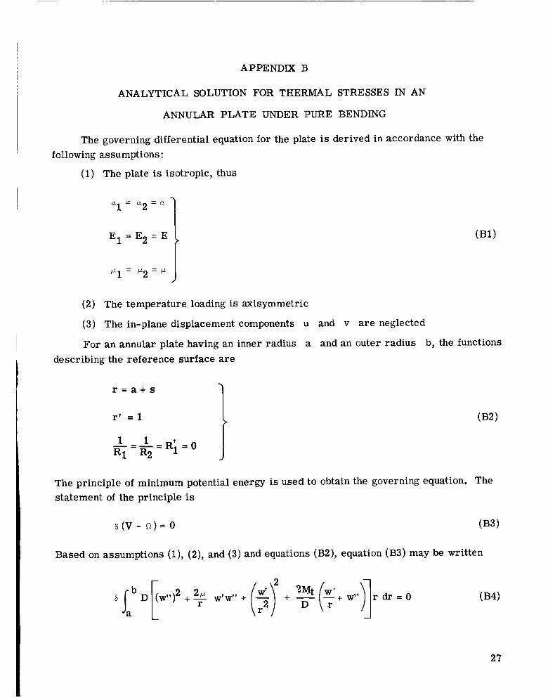
APPENDIX B

ANALYTICAL SOLUTION FOR THERMAL STRESSES IN AN

ANNULAR PLATE UNDER PURE BENDING

The governing differential equation for the plate is derived in accordance with the following assumptions :

(1) The plate is isotropic, thus

I al = a2 = a

El = E2 = E

P I = P 2 = P

(2) The temperature loading is axisymmetric

(3) The in-plane displacement components u and v are neglected

For an annular plate having an inner radius a and an outer radius b, the functions describing the reference surface a r e

7 r = a + s

r' = 1

The principle of minimum potential energy is used to obtain the governing equation. The statement of the principle is

6 (v - n ) = 0

Based on assumptions (l), (2), and (3) and equations (B2), equation (B3) may be written

27

APPENDIX B

where

D.- Eh3

and the prime indicates a derivative with respect to r. Carrying out the variations as indicated in equation (B4) yields the required differential equation

r r2 r 3 Dr

Letting the right side of equation (B5) be represented by a function M(r) and regrouping the left side yield

A solution to equation (B6) is sought which corresponds to a constant value of M. The general solution to equation (B6) with M equal to a constant is

2 2 M r 64

w = A + B r + c r l o g r + d l o g r + -

The changes in curvature and the moment resultants are then calculated by use of equa- tions (10) and (37), respectively. The boundary conditions a r e taken to be those of clamped edges

w(a) = w'(a) = 0

W(b) = w'(b) = 0

Substituting equation (B7) into equations (B8) gives the following equation for determining the constants:

28

APPENDIX B

2 l a

0 2a

1 b2

0 2b

2 a l o g a

a(1 + 2 log a)

b2 log b

b( l + 2 log b)

A

B

C

d

4 - Ma 64

- Ma3 16

- -

Mb4 -- 64

- m3 . 16 .

Return now to the determination of a temperature distribution corresponding to a constant value of M and set

-Mi - rM:

Dr = M = Constant

then the differential equation for Mtl may be written as

;Er(rq) d = -MDr

Integrating and discarding the constants of integration give

Using equation (B11) along with the expression for the thermal moment in t e rms of tem- perature (eqs. (15)) gives

29

APPENDIX B

Thus a temperature distribution corresponding to a constant value of M is one in which the temperature differewe between the inner and outer fiber of the plate varies quadrati- cally with r. Letting

T o - T . = P r 2 1

I resul ts in

and

30

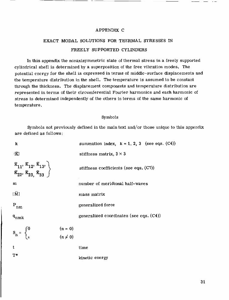
APPENDIX C

EXACT MODAL SOLUTIONS FOR THERMAL STRESSES IN

FREELY SUPPORTED CYLINDERS

In this appendix the nonaxisymmetric state of thermal s t r e s s in a freely supported cylindrical shell is determined by a superposition of the free vibration modes. The potential energy for the shell is expressed in terms of middle-surface displacements and the temperature distribution in the shell. The temperature is assumed to be constant through the thickness. The displacement components and temperature distribution a r e represented in te rms of their circumferential Fourier harmonics and each harmonic of stress is determined independently of the others in t e rms of the same harmonic of temperature.

Symbols

Symbols not previously defined in the main text and/or those unique to this appendix are defined as follows:

k summation index, k = 1. 2, 3 (see eqs. (C4))

RI stiffness matrix, 3 X 3

K22' 5 3 , R33 stiffness coefficients (see eqs. (C7))

m number of meridional half-waves

[MI mass matrix

'nm generalized force

qnmk generalized coordinates (see eqs. (C4))

s = {O " 7 7

t

T*

time

kinetic energy

31

nmk' Pnmk' ynmk a

{a)

nmk

Subscript :

n

APPENDIX C

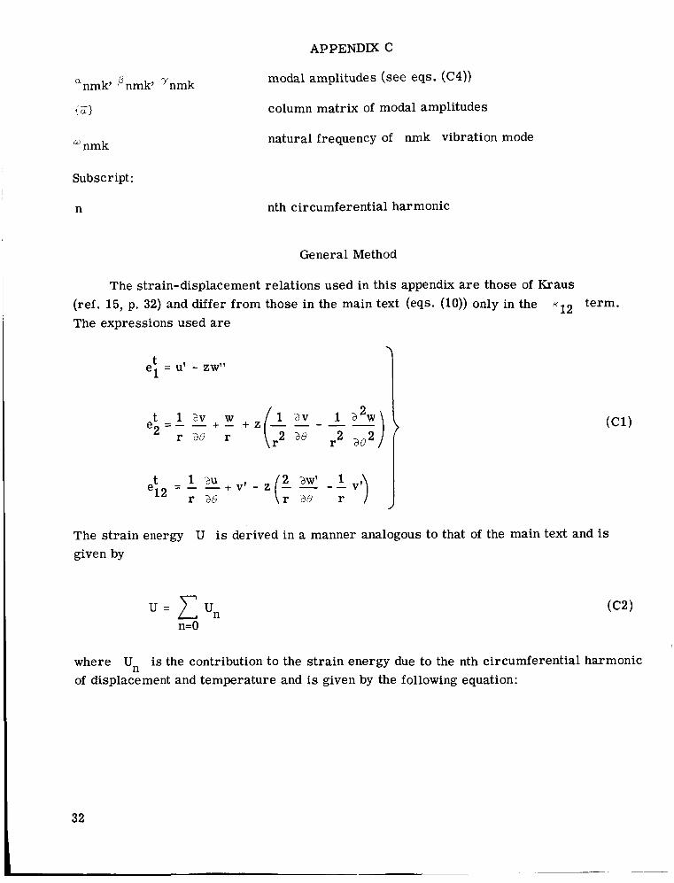
modal amplitudes (see eqs. (C4))

column matrix of modal amplitudes

natural frequency of nmk vibration mode

nth circumferential harmonic

General Method

The strain-displacement relations used in this appendix are those of Kraus (ref. 15, p. 32) and differ from those in the main text (eqS. (10)) only in the The expressions used are

K~~ term.

t el = u' - zw"

The s t ra in energy U is derived in a manner analogous to that of the main text and is given by

u = c u n n=O

where of displacement and temperature and is given by the following equation:

Un is the contribution to the s t ra in energy due to the nth circumferential harmonic

APPENDIX C

2 n2 2 wYn 2n

" 2 r r 2 r2 n n u' + - v n + - + - v w

-

2P n 2P + (2) 2 2 Un +-u'v + - u ' w n n

r r n n r

3 2 n2 2 n4 2 2n

r r r

where

(n= 0)

(n f 0) n s -(" n

In equation (C3) the first integral represents the membrane strain energy, the second integral represents the flexural strain energy, and the third integral represents the thermal strain energy.

The displacement components un(s), vn(s), and wn(s) a r e expanded in t e rms of the free vibration modes of a cylinder with freely supported edges (ref. 9). This expansion is as follows:

M 3 m n s

u p ) = pnmk cos - L qnmk m=l k = l

33

M 3 mn s vn(s) = C Pnmk sin - L qnmk

m = l k=l

M 3 mTs

w n (SI = C C ynmk s in - L qnmk m = l k=l

~ Here m represents the number of meridional half-waves in the mode shape and M is the largest value of m in the expansion. The inner summation with index k is used to account for the fact that corresponding to a given nodal pattern defined by n and m there are three modes. The relative amplitudes of un9 vn, and wn in a given mode are given by anmk9 Pnmk? and Ynrnk' respectively, and the generalized coordinate associated with a mode is denoted by qnmk. The coordinates qnmk are calculated by the principle of minimum potential energy. Substituting equations (C4) into the strain energy in equation (C3), integrating with respect to s, and minimizing the resulting expression with respect to each of the unknowns qnmk give the following formula:

where

rnr L

A m = ___

L Pnm = I, Tn(s) sin h m s ds

and the stiffness coefficients are defined as follows:

APPENDIX C

K 2 2 = - c;Lr (;2 - + c - 1 - P + - + D - - r 2

3 K 2 3 = 7 [ 7 + - + - 'nLr Cn Dn Dpn *2 + Dn(1 - p ) A 2 - -1 2 r 2 m r 4 r

2 K33 - = CnLr ?[$ + Dhm 4 + - Dn + 2pD __ n2 A 2 + 2D(1 - p ) __ n 2

4

r 2 m r 4 r r

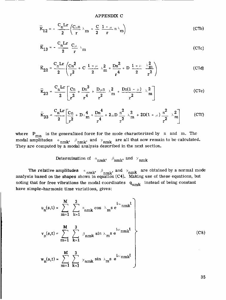
where Pmn is the generalized force for the mode characterized by n and m. The modal amplitudes They are computed by a modal analysis described in the next section.

anmk, pnmk, and Ynmk are all that now remain to be calculated.

Determination of anmk, pnmk, and ynmk

The relative amplitudes anmk, pnmk, and ynmk are obtained by a normal mode analysis based on the shapes shown in equation (C4). Making use of these equations, but noting that for free vibrations the modal coordinates qnmk instead of being constant have simple-harmonic time variations, gives:

i w t cos h m s e nmk

M 3 un(s,t) = C C a nmk

M 3 i w t nmk sin A s e n (s,t)= Pnmk m m=l k= l

35

APPENDIX C

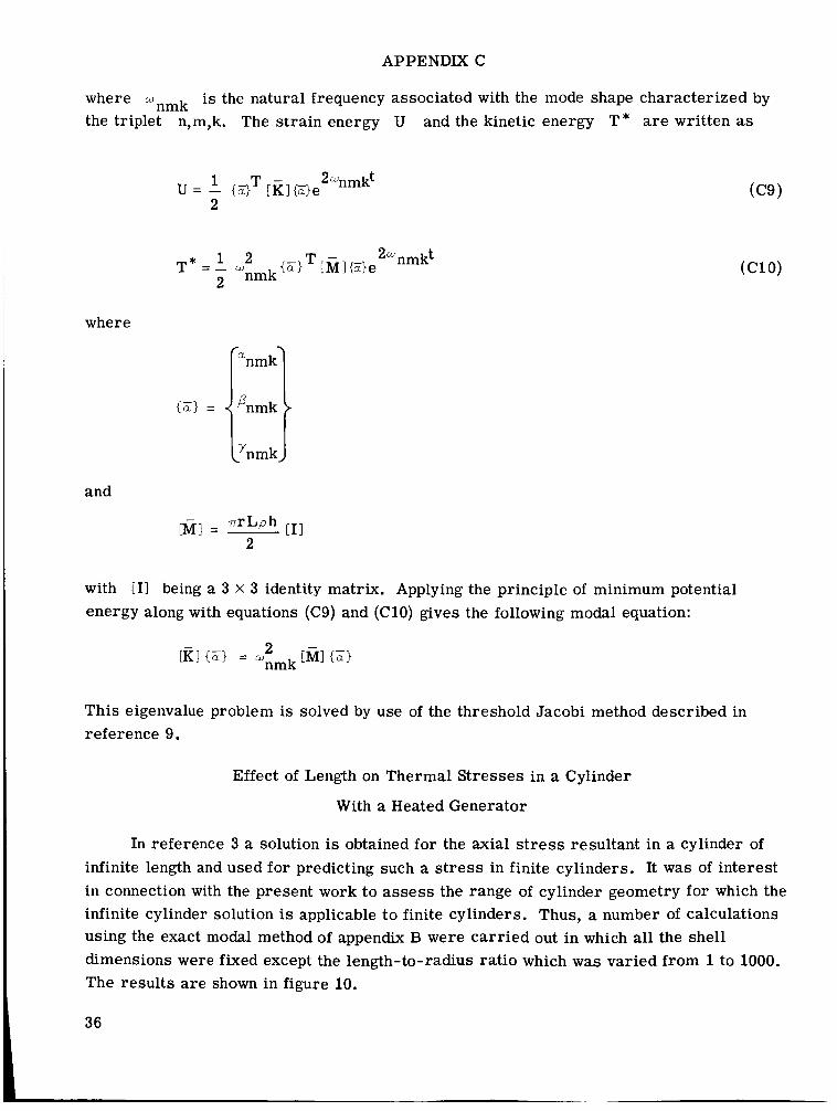
where the triplet n,m,k. The s t ra in energy U and the kinetic energy T* are written as

w n m k is the natural frequency associated with the mode shape characterized by

where

{a) =

and

nmk

Pnmk

-'nmk

a

[I3 - VrLph [MI = - 2

with [I3 being a 3 X 3 identity matrix. Applying the principle of minimum potential energy along with equations (C9) and (C10) gives the following modal equation:

This eigenvalue problem is solved by use of the threshold Jacobi method described in reference 9.

Effect of Length on Thermal Stresses in a Cylinder

With a Heated Generator

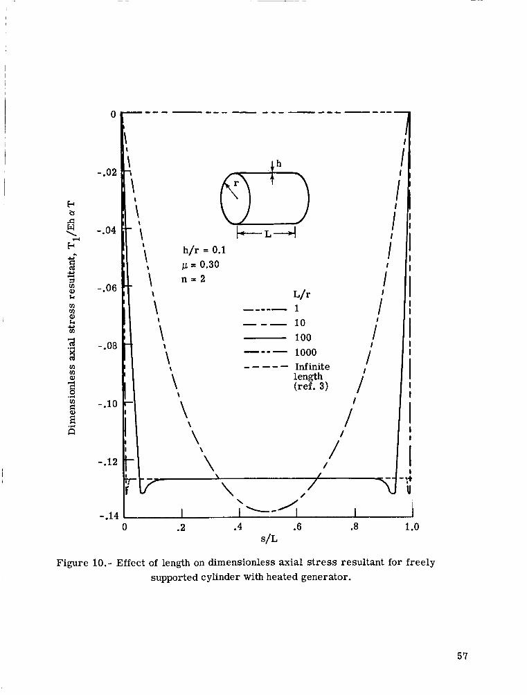
In reference 3 a solution is obtained for the axial stress resultant in a cylinder of infinite length and used for predicting such a stress in finite cylinders. It was of interest in connection with the present work to assess the range of cylinder geometry for which the infinite cylinder solution is applicable to finite cylinders. Thus, a number of calculations using the exact modal method of appendix B were carried out in which all the shell dimensions were fixed except the length-to-radius ratio which was varied from 1 to 1000. The results a r e shown in figure 10.

36

APPENDIX C

The infinite cylinder solution is denoted by the broken line. It is of course con- stant. For L/r = 1, the axial s t r e s s is 0. For L/r = 10, the curve attains a compres- sive s t r e s s at the center of the cylinder which exceeds the infinite cylinder stress by about 9 percent. For L/r = 100 and 1000, the s t ress is constant and equal to the infinite cylinder solution outside a narrow boundary layer adjacent to each edge. At the beginning of boundary layer, a value of stress is reached which exceeds the infinite-cylinder solution by about 4 percent. The conclusion from this study is that the infinite-cylinder solution is a good approximation for the s t resses in the interior of a long cylinder (L/r greater than or equal to about 100) but underestimates the stress near the edges. The infinite cylinder solution is furthermore found to be completely erroneous for cylinders having L/r less than 10.

37

REFERENCES

1. Boresi, A. P.: General Investigation of Thin Shells Including the Effect of Nonhomo- geneous Temperature Distribution. TAM Rep. No. 177 (Contract NO. NR 1834(14)), Univ. of Illinois, Aug. 1960.

2. Eisentraut, R. A.: Thermal Stresses in Cylindrical Shells. Tech. Rep. No. 112 (Con- tract Nonr 225(16)), Div. Eng. Mech., Stanford Univ., Oct. 30, 1957.

3. Ong, Chung-Chun: Effects of Thermal Stresses on Free Vibrations of Thin Cylindrical Shells. Ph. D. Diss., Northwestern Univ., Aug. 1967.

4. Bushnell, David; and Smith, Strether: Stress and Buckling of Nonuniformly Heated Cylindrical and Conical Shells. AIAA J., vol. 9, no. 12, Dec. 1971, pp. 2314-2321.

5 . Anderson, M. S.; Fulton, R. E.; Heard, W. L., Jr.; and Walz, J. E.: Stress, Buckling, and Vibration Analysis of Shells of Revolution. Computers & Structures, vol. 1, nos. 1/2, Aug. 1971, pp. 157-192.

6. Stephens, Wendell B.: Computer Program for Static and Dynamic Axisymmetric Non- linear Response of Symmetrically Loaded Orthotropic Shells of Revolution. NASA TN D-6158, 1970.

7. Cohen, Gerald A.: Computer Analysis of Asymmetrical Deformation of Orthotropic Shells of Revolution. AIAA J., vol. 2, no. 5 , May 1964, pp. 932-934.

8. MacNeal, Richard H., ed.: The NASTRAN Theoretical Manual (Level 15). NASA SP-221(01), 1972.

9 . Adelman, Howard M.; Catherines, Donnell S.; and Walton, William C-, Jr.: A Method for Computation of Vibration Modes and Frequencies of OrthotrokLc ~ i ~ i n %ells of Revolution Having General Meridional Curvature. NASA T N D-4972, 1969.

10. Adelman, Howard M.; Catherines, Donnell S.; Steeves, Ear l C.; and Walton, William C., Jr.: User's Manual for a Digital Computer Program for Computing the Vibration Characteristics of Ring-Stiffened Orthotropic Shells of Revolution. NASA TM X-2138, 1970.

11. Adelman, Howard M.; and Catherines, Donnell S.: Calculation of Temperature Distri- butions in Thin Shells of Revolution by the Finite-Element Method. NASA T N D-6100, 1971.

I

12. Adelman, Howard M.; Catherines, Donnell S.; and Walton, William C., Jr.: Accuracy of Modal Stress Calculations by the Finite Element Method. AIAA J., vol. 8, no. 3, Mar. 1970, pp. 462-468.

38

13. Boley, Bruno A.; and Weiner, Jerome H.: Theory of Thermal Stresses. John Wiley & Sons, Inc., c.1960, p. 263.

14. Huth, J. H.: Thermal Stresses in Conical Shells. J. Aeronaut. Sci., vol. 20, no. 9, Sept. 1953, pp. 613-616.

15. Kraus, Harry: Thin Elastic Shells. John Wiley & Sons, Inc., c.1967.

,

I

\

39

TABLE 1.- STIFFNESSES OF AN ORTHOTROPIC SHELL

AS USED IN EQUATION (5)

[Subscripts 1 and 2 refer to meridional and circumferential directions, respective14

dz cll = s, 1 -PIP2

2 z dz -

1 - PIP2 D1l-

z d z l - c”1/”2

K22 = I,

C66= [ G d z Jz

K66 = Gz dz

* + * + .. e- M

w * m M m

+ e-

Q, Q, k w

Q, Q,

;r:

a a z 2 Y Q, a, -

k 0 a v1 h a v1

a 0, k

4 #-I

E

I

& 9

.r(

44

v1 h a 4

E ;;i

T

k 0

? m h a m

R

4

E .rl

2 1

2: 1 4 !L2 E Q , 3 2

v a

a m

V R

a 0, a cd 0

a Q,

k 0 a a 3 m h Q, Q,

E

I 4

c,

d

E

G I k 0 a a ? m h Q, Q, k

a 0) k 0 a a 3 m h a

d

7 4

d

E tij

a a, a cd V

E

I d

a 8 k 0 a a

h a

0

2

E tij

4

a Q, +-, k 0

Q m

h Q, Q, k w

d

I

E B

a Q, a cd

a Q,

k 0 a a 3 m h a m

a

c,

d

E

I !L E B

.*

cd

41

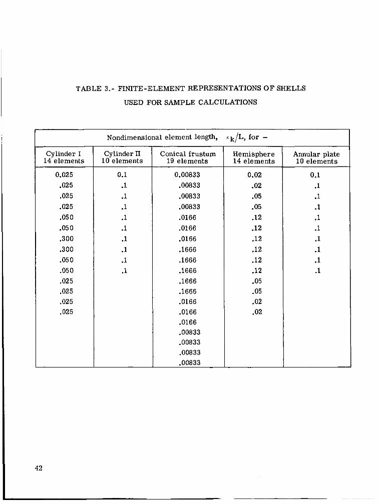
TABLE 3.- FINITE-ELEMENT REPRESENTATIONS OF SHELLS

USED FOR SAMPLE CALCULATIONS

Cylinder I 14 elements

0.025 .025 .025 .025 ,050 .050 .300 .300 .050 .050 .025 .025 .025 ,025

Nondimensional element length, E ~ / L , for -

Cylinder II 10 elements

0.1 .1 .1 .1 .1 .1 .1 .1 .1 .1

Conical frustum 19 elements

0.00833 ,00833 .00833 .00833 .0166 .0166 .0166 .1666 ,1666 ,1666 ,1666 .1666 .0166 .0166 .0166 .00833 .00833 .00833 .00833

Hemisphere 14 elements

0.02 .02 .05 .05 .12 .12 .12 .12 .12 .12 .05 .05 .02 .02

Annular plate 10 elements

0.1 .1 .1 .1 .1 .1 .1 .1 .1 .1

42

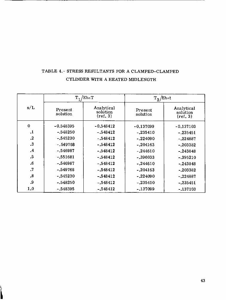
TABLE 4.- STRESS RESULTANTS FOR A CLAMPED-CLAMPED

CYLINDER WITH A HEATED MIDLENGTH

0 .1 .2 .3 .4 .5 .6 .7 .8 .9

1 .o

T. /EhaT

Present solution

- 0.548395 -.54825 0 -.545230 -.549768 - .5 4698 7 -.551681 -.546987 -.549768 -.545230 - .54825 0 -,548395

Analytic a1 solution (ref. 3)

-0.548412 - .548412 - .548412 - .548412 - .5 48 41 2 - .548412 - .548412 -.548412 -.548412 -.548412 -.5 48 412

T, h h a t

Present solution

-0.137099 -.235410 - .22 409 0 - .2 04163 - .244610 - .396033 - .244610 - .204163 -.224090 -.235410 -.137099

Analytical solution (ref. 3)

- 0.137 103 -.235451 -.224887 -.203382 -.243848 -.395210 -.243848 -.203382 - .2 2 488 7 -.2 3545 1 -.137 103

43

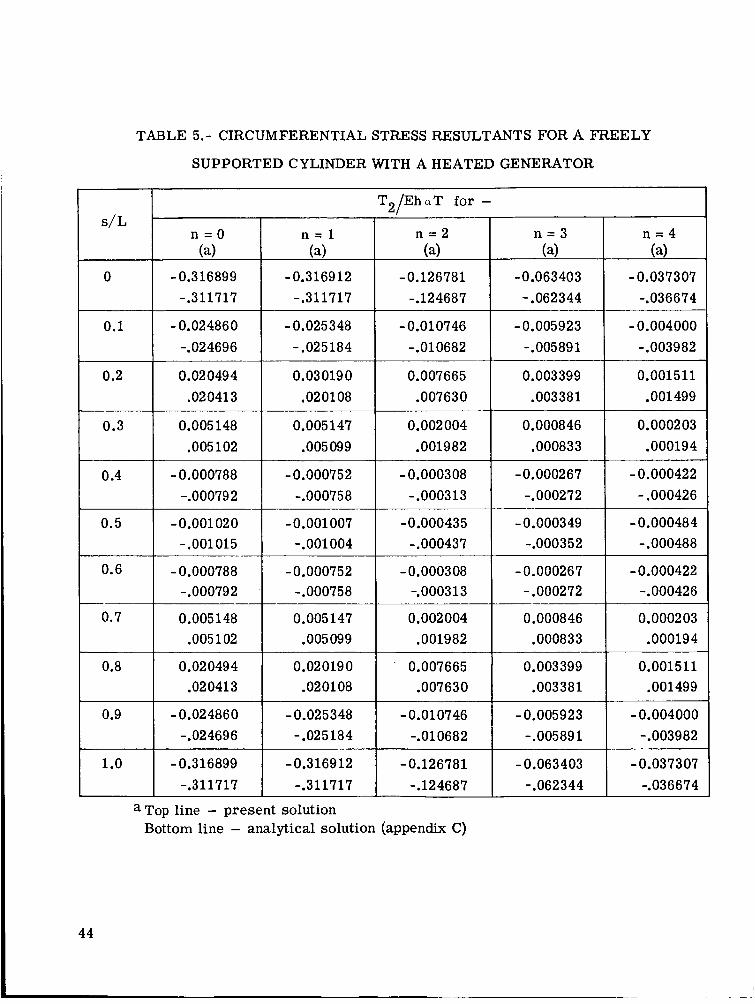
TABLE 5.- CIRCUMFERENTIAL STRESS RESULTANTS FOR A FREELY

SUPPORTEDCYLINDERWITHAHEATEDGENERATOR

T EhaT for - 2 1

- 0.126781 -0.063403 - 0.037307 -. 124687 - .062344 -.036674

s / L

0

0.1

0.2

0.3

0.4

0.5

0.6

0.7

0.8

0.9

1 .o

n = O (4

n = l (4

- 0.316912 -.311717

- 0.316899 -.311717

-0.024860 -.024696

-0.025348 -.025184

- 0.010746 -0.005923 -0.004000 - .010682 -. 005 89 1 -.003982

0.02 049 4 .020413

0.03019 0 ,020108

0.007665 0.003399 0.001 511 .007630 .003 38 1 .001499

0.002004 0.0008 46 0.000203 .001982 .000833 .000194

-0.000422 -.000313 -.000272 - ,000426

-0.000308 - 0.00026 7

0.005 148 .005102

0.005147 .005099

- 0.000788 -.000792

-0.000752 -.000758

- 0.001 02 0 - .001015

- 0.001 007 -.001004

-0.000435 -0.000349 -0.000484 - .000437 -.000352 - .000488

- 0.000788 -. 00079 2

-0.000752 -. 00075 8

-0.000308 - 0.000267 -0.000422 -.0003 13 - .000272 -.000426

0.005148 .005102

0.005 147 .005099

0.002 004 0.000846 0.0002 03 .001982 .000833 .000194

0.020494 .02 041 3

0.02 019 0 ,0201 08

0.003399 0.00151 1

-0.005923 - 0.004000 -.010682 - .00589 1 - .0039 82

-0.024860 -.02 469 6

-0.025348 -.025184

-0.316899 -.311717

-0.316912 -.311717

-0.126781 -0.063403 -0.037307 -. 03 6 6 7 4 -.124687 - .062 3 44

a Top line - present solution Bottom line - analytical solution (appendix C)

44

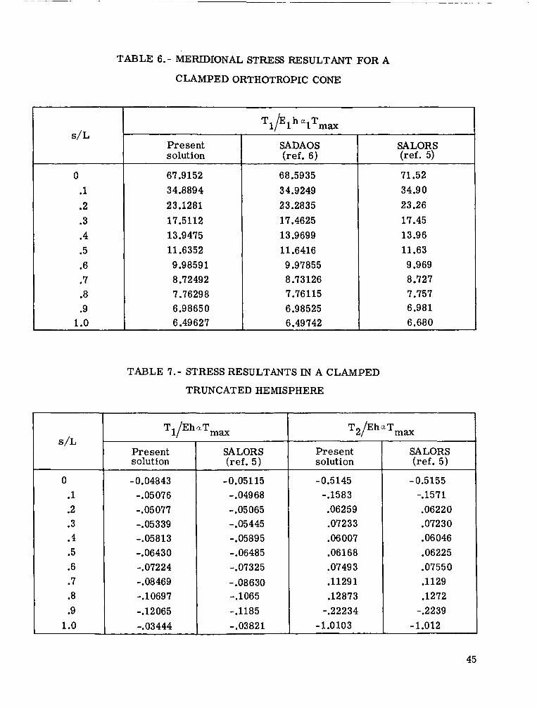
TABLE 6.- MERIDIONAL STRESS RESULTANT FOR A

CLAMPED ORTHOTROPIC CONE

0 .1 .2 .3 .4 .5 .6 .7 .8 .9

1 .o

s/L

0 .1 .2 .3 .4 .5 .6 .7 .8 .9

1 .o

Present solution

67.9152 34.8894 23.1281 17.5112 13.9475 11.6352 9.9859 1 8.72492 7.76298 6.98650 6.49627

SADAOS (ref. 6)

68.5935 34.9249 23.2835 17.4625 13.9699 11.6416 9.97855 8.73126 7.761 15 6.98525 6.49 742

SALORS (ref. 5)

71.52 34.90 23.26 17.45 13.96 11.63 9.969 8.727 7.757 6.981 6.680

TABLE 7.- STRESS RESULTANTS IN A CLAMPED

TRUNCATED HEMISPHERE

T EhaTrnax 11

Present solution

- 0.04843 -.05 076 -.05077 -.05339 -.05813 -. 0643 0 -.07224 -.08469 -.lo697 -. 12 065 -.03444

SALORS (ref. 5)

- 0.05 115 - .04968 - .05 065 -.05445 -.05895 - .06485 -.07325 -.08630 -.lo65 -.1185 -.03821

T EhaTmax 21

Present solution

-0.5145 -.1583 .06259 .07233 .06007 ,06168 .07493 .11291 .12873 -.22234

- 1 .O 103

SALORS (ref. 5)

-0.5155 -.1571 .06220 .07230 .06046 .06225 .07550 .1129 .1272 -.2239

-1.012

45

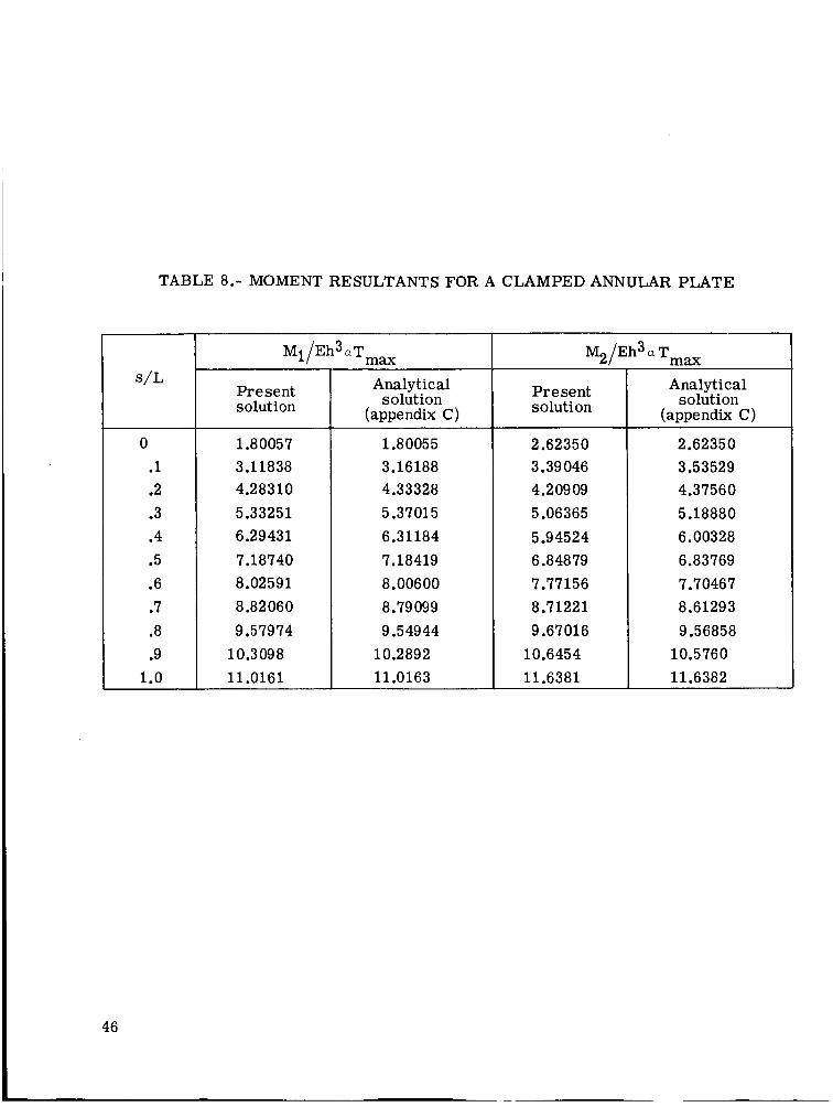
TABLE 8.- MOMENT RESULTANTS FOR A CLAMPED ANNULAR PLATE

0 .1 .2 .3 .4 .5 .6 .7 .8 .9

1.0

46

Mi /Eh3aTmax AI

Present solution

1.80057 3.11838 4.28310 5.33251 6.29431 7.18740 8,02591 8.82060 9.57974

1 0.3 09 8 11.0161

Analytic a1 solution

(appendix C)

1.80055 3.16188 4.33328 5.3701 5 6.31 184 7.18419 8.00600 8.79 099 9.54944

10.2892 11.0163

M2/Eh3 a Tmax

Present solution

2.62350 3.39 046 4.2 09 09 5.06365 5.94524 6.84879 7.77156 8.71221 9.67016

10.6454 11.6381

Analytical solution

(appendix C)

2.62350 3.53529 4.37560 5.18880 6.00328 6.83769 7.70467 8.61293 9.56858

10.5 76 0 11.6382

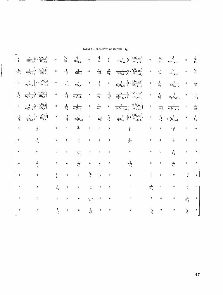
TABLE 9.- ELEMENTS OF MATRIX [Tk]

o - - 5Sk ‘f 0 - 1 . ‘k l + ‘ k % , k + l ) 32 64R1,k 64 32Ri,k+i 2Rl ,k+l

0 -3 -1 0 . 4Ek %,k

1 1 (. + ‘kR;,k+l\ 8 4ckRi ,k+i \ 2 R l , k + l /

0 2- -1 4‘k ’%.k+l

0 0 0 0 0 ‘k 1 - 8 2

‘k .- 0 0 8

0 0 0 0 1 4

0 0 0 3 ” k

.- - 1 0 0 _ _ 4

3 “ k .-

O O I

0 0 ._ 0 0 0 0 1

” k 0 0

2 l o z 1 0 0 -

6;

f o 0 0 0

0 0 - 3 0 0 “ k

__ 3 0 0 -1 0 0 0 k

0 0 0 __ l o o 0 “ k

l o 0 0 0 0

i o 0

.- 2 o f f

0 0 l o o 0 6%

47

(a) Coordinate system and displacement component directions.

kr3$ $+ 4

(b) Detail of shell wall.

Figure 1.- Geometry of a shell of revolution.

48

E * 10 GPa (Y = 1 x I O - ~ / K h r 1 0 c m p = 0.25

r = 1.0 m L t 1.0 m

sinh (s/L)

sinh (1-s/L)

sinh (1/2)

sinh (l/aj (0 2 s/L I 1/21 To=T. =

1

(1/2 2 s/L 2 1)

(a) Cylinder with heated midlength - clamped edges (cylinder I).

h r l c m L = 1 . 0 m CT = 1 X 10-6/K r = 1.0 m E = 10 GPa p * 0.3

- t anhn ( n = O )

~ ( 1 t n )

To= Ti= C T cos ne 1 n II

2 t a n h a (n.0) T =

(b) Cylinder with heated generator - freely supported edges (cylinder II).

h = 0.0625 cm To= 1500 - 1000 (s/L) + 500 (s/L)’ Ti = 500

~1 0.25 r mln . t 6 0 c m 4 = 0.20 r 4” El = 50GPa 01 = 6.67 X 10-6/K ‘min I+ E2 = 40 GPa cy2 = 6.08 x 1 0 - 6 / ~

(c) Conical frustum - clamped edges.

h = l c m L = l . O m p = 0.3 a = 1.0 m

E = 10 GPa

(Y = 1 X 10-6/K

R = 0.540 m

(d) Truncated hemisphere - clamped edges.

a = 1.0m (Y = 1 x I O - ~ / K

L = r 2 - rl p = 0.3

2 E = 100 GPa To-Ti 2000 (1 + s/L)

(e) Annular plate - clamped edges.

Figure 2 . - Models used for sample calculations. All temperatures are in K.

49

I

E-c a G w E-c

-.5

a

E a G -.4 w E-c - \ rn

3 5 -.3 5 rn W k rn rn W k c,

rn rn W

r-0 -.2

4

.d b rn

0 Present solution - Exact solution (ref. 3)

0 .2 .4 .6 .8 1 .o s/L

Figure 3 . - Stress resultants in cylinder with prescribed midlength temperature. Both edges clamped; cylinder I.

50

E el G w E \ ., 5 t: i2 W k m m W k m u

.2

.1

0

1

<

-.l 1

-.2

-.3 (

- .4

' LT =Constant

Present solution 0 n = 0 , 1 17 n = 2 0 n e 3 A n = 4

Exact solution (appendix C)

0 .1 .2 .3 .4 .5 s/L

Figure 4. - Circumferential s t r e s s resultant in cylinder with heated generator. Both edges clamped.

51

.2

0

-.2

-.4 I

-.6

-.8

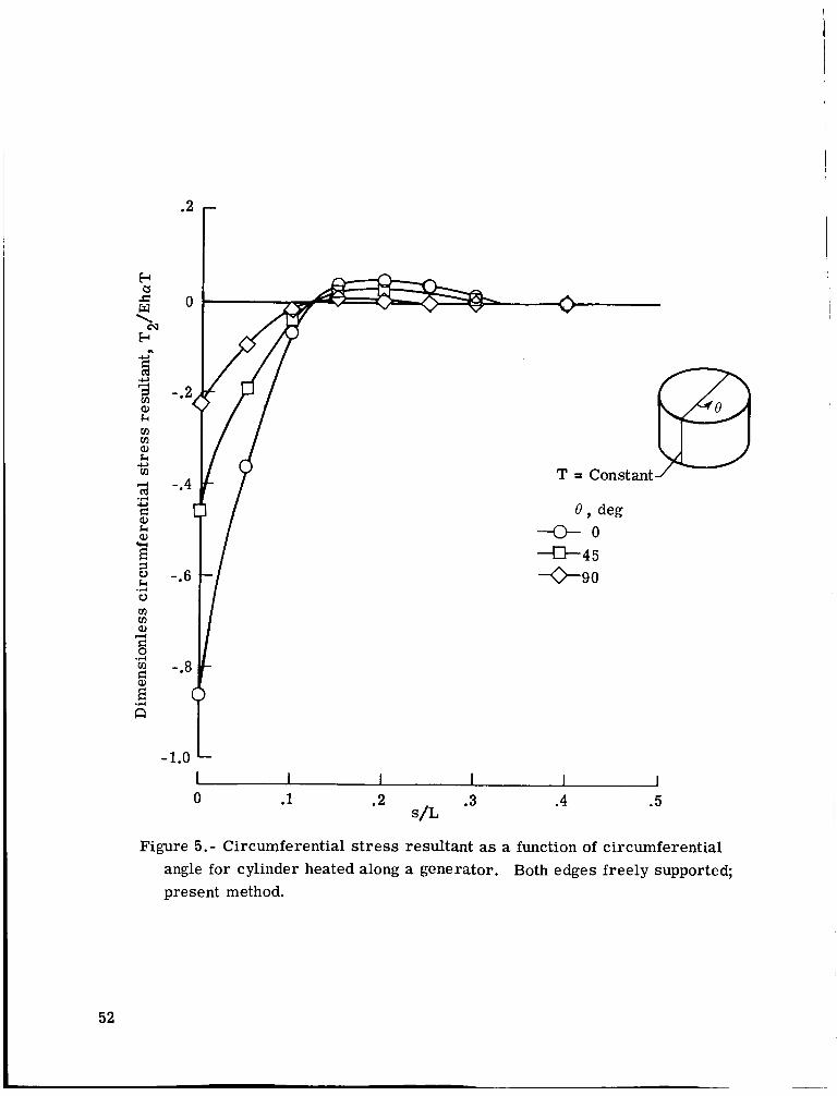
-1.0 I I I I I 1 0 .1 .2 .3 .4 . 5

s/L

Figure 5. - Circumferential s t r e s s resultant as a function of circumferential angle for cylinder heated along a generator. Both edges freely supported; present method.

52

-80

4 - 70 I

-60

- 50

-40

-30

- 20

-10

0

L

I

h a3 Both edges clamped

Present solution --@--- SADAOS (ref. 6) --e- SALORS (ref. 5)

I 1 I 1 I .2 .4 .6 .8 1 .o

s/L

Figure 6.- Meridional s t r e s s resultant in orthotropic 300 conical frustum. Both edges clamped; To = 1500 - lOOO(s/L) + 5 0 0 ( ~ / L ) ~ ; Ti = 500.

53

3 E 1.0 E tl G w E a 0.5 \

3 E

E

w E

c a O I

\ - m

-0.5( I4 3 m a, k m m a, k m m m

-y -1.0

A

/ n v U / \ - P

\ A LMerid iona l resultant

L c i r cumferent id / result ant \ . \

Present solution O-l

Reference 5 -

6 I4 s

E

.?I m $ -1.5

I I I I 0 .2 .4 .6 .8 1 .o

s/L

Figure 7.- Stress resultants in truncated hemisphere. Both edges clamped;

To = Ti = 1 + 0.6587 log

54

12.5

10.0 3 3 VI a, k 42

7.5

s VI VI a,

3 5.0 .r( VI : 5

2.5

P

Meridional r e sult ant, M1/Eh 3 (Y (To- T.)

1 max 0 Present solution

Exact solution

Circumferential resultant, M2/Eh 3 cy (To- T.)

1 max 0 Present solution

---- Exact solution

I I 1 I I 0 .2 .4 .6 .8 1.0

sAb-4

Figure 8.- Moment resultants in annular plate. Both edges clamped;

TO = Ti = 2000

55

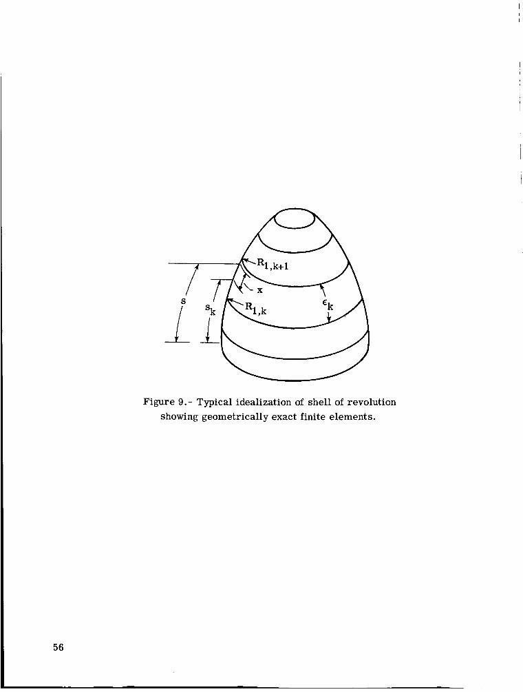
‘1 ,k+l

Figure 9.- Typical idealization of shell of revolution showing geometrically exact finite elements.

56

0

-.02

c w \ -.04 E”

5 -

24 v) Q) -.06 7

k m v) Q) k c, m

-.08 ‘9 m m : 0 .#-I

-.lo m E b“ E

-.12

-.14

\

\ \

- \ \

i

I

I

I

t

\ \ \ \ \

\

\

l h

I I I

I I

I

h/r = 0.1

n - 2 p = 0.30 I

I L/r ----- 1 --- 10 i

I 100

\ \

\ \

\ \ \

i 1000

length

---- ----- Infinit e

I

/

/ /

I I

I

I I I

I I

I I

I

i I I

I I

I I

I t 1

0 .2 .4 .6 .8 1 .o s/L

Figure 10.- Effect of length on dimensionless axial stress resultant for freely supported cylinder with heated generator.

57