Anisoplanatic Wavefront Error Estimation using Coherent Imaging

The phase retrieval problem A convex approach Illumination strategies Conclusions
Coherent imaging without phases
Miguel Moscoso ∗
∗Joint work with Alexei Novikov Chrysoula Tsogka and George Papanicolaou
Waves and Imaging in Random Media, September 2017

The phase retrieval problem A convex approach Illumination strategies Conclusions
Outline
1 The phase retrieval problem
2 A convex approach
3 Illumination strategies
4 Conclusions

The phase retrieval problem A convex approach Illumination strategies Conclusions
Motivation
In many situations it is difficult, or impossible, to measure the phases.Only the intensities are available for imaging!
X-ray cristalographyTHz radar & imaging systemsDiffraction imagingAstronomical imaging...
COHERENT WAVE PROPAGATION

The phase retrieval problem A convex approach Illumination strategies Conclusions
The significance of phase
Atletico de Madrid
Real Madrid
Figure: Atletico de Madrid soccer shield (top) and Real Madrid soccer shield(bottom).

The phase retrieval problem A convex approach Illumination strategies Conclusions
Motivation
FFT Magnitude ATM FFT Phase ATM
FFT Magnitude RM FFT Phase RM
Figure: Magnitudes and phases of Atletico (top row) and Real Madrid(bottom row) soccer shields.
The phase retrieval problem A convex approach Illumination strategies Conclusions
Motivation
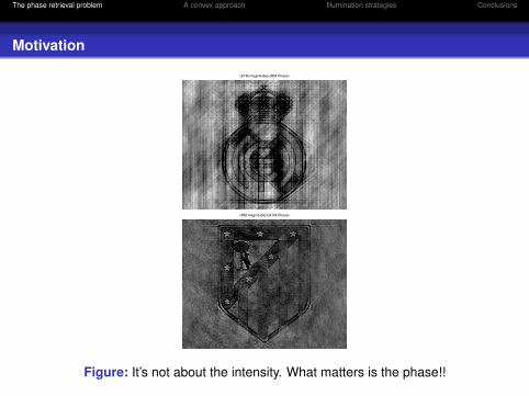
(ATM magnitude)x(RM Phase)
(RM magnitude)x(ATM Phase)
Figure: It’s not about the intensity. What matters is the phase!!

The phase retrieval problem A convex approach Illumination strategies Conclusions
The phase retrieval problem
Mathematically ...
... the phase retrieval problem consists of recovering an unknownsignal x[n] from the amplitude |x[k]| of its Fourier transform
x[k] =
N∑n=1
x[n] e−i2πkn/N , k = 1, . . . , N .

The phase retrieval problem A convex approach Illumination strategies Conclusions
The phase retrieval problem
Mathematically ...
... the phase retrieval problem consists of finding the phases thatsatisfy a set of linear constraints for the measured amplitudes
| < x, ak > |2 = |bk|2 .

The phase retrieval problem A convex approach Illumination strategies Conclusions
The phase retrieval problem: algorithms
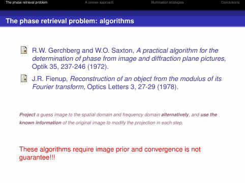
R.W. Gerchberg and W.O. Saxton, A practical algorithm for thedetermination of phase from image and diffraction plane pictures,Optik 35, 237-246 (1972).
J.R. Fienup, Reconstruction of an object from the modulus of itsFourier transform, Optics Letters 3, 27-29 (1978).
Project a guess image to the spatial domain and frequency domain alternatively, and use the
known information of the original image to modify the projection in each step.
These algorithms require image prior and convergence is notguarantee!!!
The phase retrieval problem A convex approach Illumination strategies Conclusions
The phase retrieval problem: algorithms
R.W. Gerchberg and W.O. Saxton, A practical algorithm for thedetermination of phase from image and diffraction plane pictures,Optik 35, 237-246 (1972).
J.R. Fienup, Reconstruction of an object from the modulus of itsFourier transform, Optics Letters 3, 27-29 (1978).
Project a guess image to the spatial domain and frequency domain alternatively, and use the
known information of the original image to modify the projection in each step.
These algorithms require image prior and convergence is notguarantee!!!

The phase retrieval problem A convex approach Illumination strategies Conclusions
The phase retrieval problem
Goal: To devise other approaches that guarantee convergence to theexact solution without prior information.

The phase retrieval problem A convex approach Illumination strategies Conclusions
The phase retrieval problem
Assume that imaging can be formulated as a linear inverse problem
Afρ = bf .
Here, Af ∈ CN×K is the model matrix that relates the unknownvector ρ ∈ CK to the data vector bf ∈ CN . Usually N K!

The phase retrieval problem A convex approach Illumination strategies Conclusions
The phase retrieval problem
Imaging WITH phases
Find ρ ∈ CK fromAfρ = bf ,
given the data vector bf ∈ CN with both amplitudes and phases.

The phase retrieval problem A convex approach Illumination strategies Conclusions
The phase retrieval problem
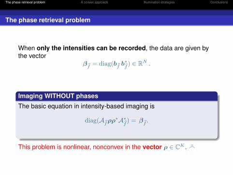
When only the intensities can be recorded, the data are given bythe vector
βf = diag(bf b∗f) ∈ RN .
Imaging WITHOUT phases
The basic equation in intensity-based imaging is
diag(Afρρ∗A∗
f) = βf .
This problem is nonlinear, nonconvex in the vector ρ ∈ CK . _
The phase retrieval problem A convex approach Illumination strategies Conclusions
The phase retrieval problem
When only the intensities can be recorded, the data are given bythe vector
βf = diag(bf b∗f) ∈ RN .
Imaging WITHOUT phases
The basic equation in intensity-based imaging is
diag(Afρρ∗A∗
f) = βf .
This problem is nonlinear, nonconvex in the vector ρ ∈ CK . _

The phase retrieval problem A convex approach Illumination strategies Conclusions
A convex approach
KEY: Replaced the nonlinear vector problem by a linear matrix one. Introduce
The decision variable X := ρρ∗ ∈ CK×K , and the
operator Lf
: CK×K → RN , such that Lf(X ) := diag(A
fXA∗
f).
Imaging WITHOUT phases
Then, at the matrix level, the equation in intensity-based imaging is
Lf (X ) = βf .
The quadratic measurements on ρ become linear on X := ρρ∗!

The phase retrieval problem A convex approach Illumination strategies Conclusions
A convex approach
Rank minimizationSolve the following rank minimization problem
min rank(X ) subject to Lf (X ) = βf , X ≥ 0.
This problem is still nonconvex!!! _
Relax!Solve the following trace minimization problem
min trace(X ) subject to Lf (X ) = bI , X ≥ 0.
This makes the problem convex and solvable in polynomial time. ¨

The phase retrieval problem A convex approach Illumination strategies Conclusions
A convex approach
A. Chai, M. Moscoso, G. Papanicolaou, Array imaging usingintensity-only measurements, Inverse Problems 27 (2011).
E. J. Candes, Y. C. Eldar, T. Strohmer, V. Voroninski, PhaseRetrieval via Matrix Completion, SIAM Journal on ImagingSciences 6 (2013).
The phase retrieval problem A convex approach Illumination strategies Conclusions
A convex approach: algorithm
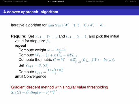
Iterative algorithm for min trace(X ) s. t. Lf (X ) = bI .
Require: Set Y−1 = Y0 = 0 and t−1 = t0 = 1, and pick the initialvalue for step size β.repeat
Compute weight w = tk−1−1tk
.Compute Wk = (1 + w)Yk − wYk−1.Compute the matrix G = W − βL∗
f(ω)(Lf(ω)(W )− bI(ω)).
Set Yk+1 = Sτ (G).
Compute tk+1 =1+√
1+4t2k2 .
until Convergence
Gradient descent method with singular value thresholdingSτ (G) = Udiag(σ − τ)+V
∗.

The phase retrieval problem A convex approach Illumination strategies Conclusions
A convex approach: algorithm
J.F. Cai, E.J. Candès, and Z. Shen, A Singular ValueThresholding Algorithm for Matrix Completion, SIAM J. Optim. 20(2008).
K.C. Toh and S. Yun, An accelerated proximal gradient algorithmfor nuclear norm regularized least squares problems, Pacific J.Optimization 6 (2010).

The phase retrieval problem A convex approach Illumination strategies Conclusions
Numerical simulations: active array imaging
Let us consider the problem of active array imaging ...

The phase retrieval problem A convex approach Illumination strategies Conclusions
Schematic for active array imaging
b
b
b
b
b
b
b
b
b
b
b
b
b
b
b
b
b
b
b
b
b
b
b
xr
xs
yj
Figure: We want to determine the location and reflectivities of (small orextended) reflectors by sending probing signals from the array and recordingthe backscattered signals. Only the intensities are recorded, in our case!

The phase retrieval problem A convex approach Illumination strategies Conclusions
Data model
We consider a region of interest: the Image Window IW.
b
b
b
b
b
b
b
b
b
b
b
b
b
b
b
b
b
b
b
b
b
b
b
xr
xs
yj
We define a grid yj , j = 1, . . . ,K, a discretization of the IW and seekto determine the reflectivities on this grid ρj = ρ(yj), j = 1, . . . ,K.
Our unknown is the vector ρ ∈ CK ,
ρ = [ρ1, . . . , ρK ]t ∈ CK , ρj = ρ(yj), j = 1, . . . ,K.
The phase retrieval problem A convex approach Illumination strategies Conclusions
The data model
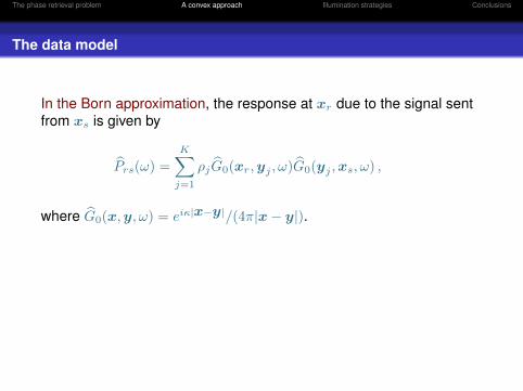
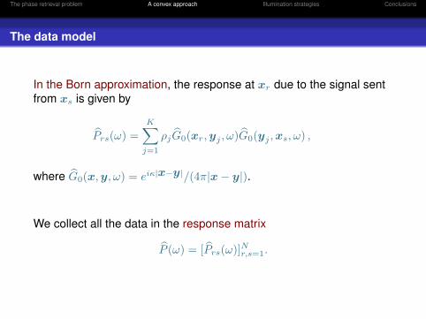
In the Born approximation, the response at xr due to the signal sentfrom xs is given by
Prs(ω) =
K∑j=1
ρjG0(xr,yj , ω)G0(yj ,xs, ω) ,
where G0(x,y, ω) = eiκ|x−y|/(4π|x− y|).
We collect all the data in the response matrix
P (ω) = [Prs(ω)]Nr,s=1.
The phase retrieval problem A convex approach Illumination strategies Conclusions
The data model
In the Born approximation, the response at xr due to the signal sentfrom xs is given by
Prs(ω) =
K∑j=1
ρjG0(xr,yj , ω)G0(yj ,xs, ω) ,
where G0(x,y, ω) = eiκ|x−y|/(4π|x− y|).
We collect all the data in the response matrix
P (ω) = [Prs(ω)]Nr,s=1.

The phase retrieval problem A convex approach Illumination strategies Conclusions
The data model
If f = [f1, . . . , fN ]T is the illumination vector, then the data bf(including phases!!!) at the array is given by
bf = P f .
Through P f , we define the model matrix
Afρ = P f ,
with [Af]rk
= G(xr,yk, ω)
N∑s=1
fsG(yk,xs, ω) .
for r = 1, . . . , N, k = 1, . . . ,K.

The phase retrieval problem A convex approach Illumination strategies Conclusions
Numerical simulations: examples I
x (λ units)
y (
λ u
nits)
85 90 95 100 105 110
10
5
0
−5
−100
0.2
0.4
0.6
0.8
1
x (λ units)
y (
λ u
nits)
85 90 95 100 105 110
10
5
0
−5
−100
0.2
0.4
0.6
0.8
1
(a) (b)
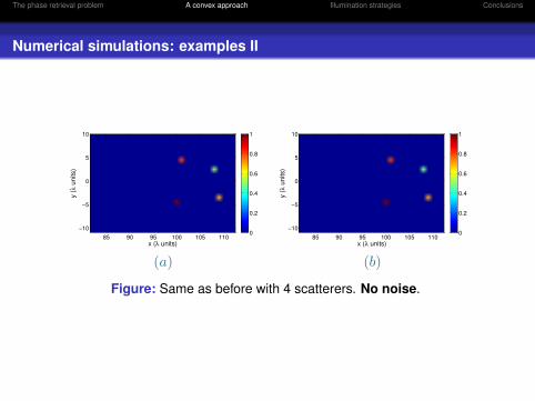
Figure: (a) Original configuration. 21 transducers. 10× 10 pixels in IW. Gridpoints separated by 1. a/L = 1. Single illumination. (b) Numerical result bysolving trace minimization with no noise.
In all the images we normalize the spatial units by λ.
The phase retrieval problem A convex approach Illumination strategies Conclusions
Numerical simulations: examples II
x (λ units)
y (
λ u
nits)
85 90 95 100 105 110
10
5
0
−5
−100
0.2
0.4
0.6
0.8
1
x (λ units)
y (
λ u
nits)
85 90 95 100 105 110
10
5
0
−5
−100
0.2
0.4
0.6
0.8
1
(a) (b)
Figure: Same as before with 4 scatterers. No noise.

The phase retrieval problem A convex approach Illumination strategies Conclusions
Numerical simulations: examples III
x (λ units)
y (
λ u
nits)
1 5 10 15 20 25 30
20
15
10
5
10
0.2
0.4
0.6
0.8
1
x (λ units)
y (
λ u
nits)
1 5 10 15 20 25 30
20
15
10
5
10
0.2
0.4
0.6
0.8
1
(a) (b)
Figure: Same as before with 65 scatterers. No noise.
Sparsity is not required!

The phase retrieval problem A convex approach Illumination strategies Conclusions
Numerical simulations: examples IV
x (λ units)
y (
λ u
nits)
85 90 95 100 105 110
10
5
0
−5
−100
0.2
0.4
0.6
0.8
1
x (λ units)
y (
λ u
nits)
85 90 95 100 105 110
10
5
0
−5
−10
0.05
0.1
0.15
0.2
0.25
(a) (b)
x (λ units)
y (
λ u
nits)
85 90 95 100 105 110
10
5
0
−5
−100
0.2
0.4
0.6
0.8
1
x (λ units)
y (
λ u
nits)
85 90 95 100 105 110
10
5
0
−5
−100
0.2
0.4
0.6
0.8
1
(c) (d)
Figure: 0.5% noise. (a) Original configuration. (b) 1 illumination. (c) 5illuminations. (d) 10 illuminations.
The number of illuminations is increased to make the method robust.

The phase retrieval problem A convex approach Illumination strategies Conclusions
A convex approach
Goal accomplished: The method guarantees exact reconstructionswithout image prior.
Drawback: It is VERY computationally expensive for large scaleproblems. Images with K of pixels require the solution of a K ×Koptimization problem.
Next goal: To devise another approach that guarantees convergenceto the exact solution and, at the same time, keep the size of theproblem small so the solution can be found more efficiently.

The phase retrieval problem A convex approach Illumination strategies Conclusions
The time reversal operator
Main ideaImaging with intensity-only can be carried out using the time reversaloperator
M = P∗P ,
which can be obtained from intensity measurements using anappropriate illumination strategy and the polarization identity.
The images can be formed using its SVD.
The phase retrieval problem A convex approach Illumination strategies Conclusions
The time-reversal operator with the polarization identity
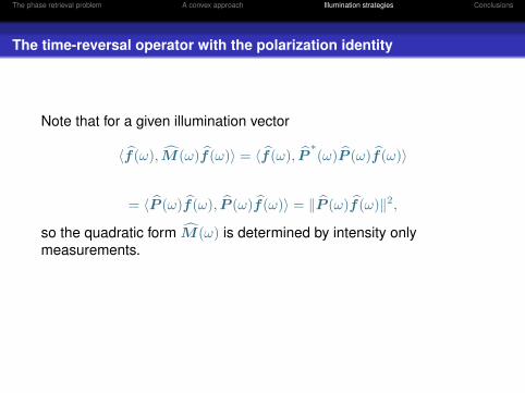
Note that for a given illumination vector
〈f(ω),M(ω)f(ω)〉 = 〈f(ω), P∗(ω)P (ω)f(ω)〉
= 〈P (ω)f(ω), P (ω)f(ω)〉 = ‖P (ω)f(ω)‖2,
so the quadratic form M(ω) is determined by intensity onlymeasurements.
Use the polarization identity
2〈x,y〉 = ‖x+ y‖2 − ‖x‖2 − ‖y‖2 + i(‖x− iy‖2 − ‖x‖2 − ‖y‖2
).

The phase retrieval problem A convex approach Illumination strategies Conclusions
The time-reversal operator with the polarization identity
Note that for a given illumination vector
〈f(ω),M(ω)f(ω)〉 = 〈f(ω), P∗(ω)P (ω)f(ω)〉
= 〈P (ω)f(ω), P (ω)f(ω)〉 = ‖P (ω)f(ω)‖2,
so the quadratic form M(ω) is determined by intensity onlymeasurements. Use the polarization identity
2〈x,y〉 = ‖x+ y‖2 − ‖x‖2 − ‖y‖2 + i(‖x− iy‖2 − ‖x‖2 − ‖y‖2
).

The phase retrieval problem A convex approach Illumination strategies Conclusions
The time-reversal operator with the polarization identity
The i-th entry in the diagonal Mii is just the total power received atthe array when only the i-th transducer fires a signal.
The off-diagonal terms Mij , i 6= j can be found as follows:
Re(Mij(ω)) = Re(Mji(ω)) =1
2
(‖P (ω)ei+j‖2 − ‖P (ω)ei‖2 − ‖P (ω)ej‖2
)
Im(Mij(ω)) = −Im(Mji(ω)) =1
2
(‖P (ω)ei−ij‖2 − ‖P (ω)ei‖2 − ‖P (ω)ej‖2
)using the illumination vectors ei+j = ei + ej and ei−ij = ei − iej .
Conclusion: With enough illuminations (N2 of them) we can obtainM(ω). Since only the total power received at the array is involved,the method very robust.

The phase retrieval problem A convex approach Illumination strategies Conclusions
Imaging without phases
Key ideas:(i) The time reversal matrix M = P
∗P and P , share the same right
singular vectors.
P (ω) = U(ω)Σ(ω)V∗(ω) =
M∑j=1
σj(ω)Uj(ω)V∗j (ω) ,
M(ω) = V (ω)Σ2(ω)V
∗(ω) =
M∑j=1
σ2j (ω)Vj(ω)V
∗j (ω) .

The phase retrieval problem A convex approach Illumination strategies Conclusions
Imaging without phases
Key ideas:(i) The time reversal matrix M = P
∗P and P , share the same right
singular vectors. Hence,MUSIC can be applied, without any modification, once M hasbeen obtained.
MUSIC algorithm
A scatterer location corresponds to a peak of the functional
I(ys) =1∑N
j=M+1 |gT0 (ys)Vj |2
, s = 1, . . . , K.
The phase retrieval problem A convex approach Illumination strategies Conclusions
Imaging without phases
Key ideas:(i) The time reversal matrix M = P
∗P and P , share the same right
singular vectors. Hence,
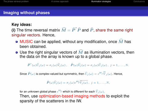
MUSIC can be applied, without any modification, once M hasbeen obtained.Use the right singular vectors of M as illumination vectors, thenthe data on the array is known up to a global phase.
P∗(ω)Uj(ω) = σj(ω)Vj(ω) , P (ω)Vj(ω) = σj(ω)Uj(ω) , j = 1, . . . , N.
Since P (ω) is complex-valued but symmetric, then Uj(ω) = eiθj V j(ω). Hence,
P (ω)Vj(ω) = σj(ω)eiθj Vj(ω) , j = 1, . . . , N,
for an unknown global phase eiθj which is different for each Vj(ω).
Then, use optimization-based imaging methods to exploit thesparsity of the scatterers in the IW.

The phase retrieval problem A convex approach Illumination strategies Conclusions
Imaging without phases
Advantages:Simple and efficientDoes not need prior informationGuarantees exact recovery in the noise-free caseIt is robust with respect to additive noise.
Drawback: The data acquisition process is expensive (N2)... but canbe minimized
using matrix completion, oredge illuminations, orinstead use the intensities at each receiver (3N − 2), orFresnel and Fraunhofer regimes (exactly 6).
Corollary (Fraunhofer): A "vector" can be determined from theabsolute value of its Fourier coefficients (its DFT) if six versions of itare known, regardless of its size.

The phase retrieval problem A convex approach Illumination strategies Conclusions
Imaging without phases
Advantages:Simple and efficientDoes not need prior informationGuarantees exact recovery in the noise-free caseIt is robust with respect to additive noise.
Drawback: The data acquisition process is expensive (N2)... but canbe minimized
using matrix completion, oredge illuminations, or
instead use the intensities at each receiver (3N − 2), orFresnel and Fraunhofer regimes (exactly 6).
Corollary (Fraunhofer): A "vector" can be determined from theabsolute value of its Fourier coefficients (its DFT) if six versions of itare known, regardless of its size.

The phase retrieval problem A convex approach Illumination strategies Conclusions
Imaging without phases
Advantages:Simple and efficientDoes not need prior informationGuarantees exact recovery in the noise-free caseIt is robust with respect to additive noise.
Drawback: The data acquisition process is expensive (N2)... but canbe minimized
using matrix completion, oredge illuminations, orinstead use the intensities at each receiver (3N − 2), orFresnel and Fraunhofer regimes (exactly 6).
Corollary (Fraunhofer): A "vector" can be determined from theabsolute value of its Fourier coefficients (its DFT) if six versions of itare known, regardless of its size.

The phase retrieval problem A convex approach Illumination strategies Conclusions
Imaging without phases
Advantages:Simple and efficientDoes not need prior informationGuarantees exact recovery in the noise-free caseIt is robust with respect to additive noise.
Drawback: The data acquisition process is expensive (N2)... but canbe minimized
using matrix completion, oredge illuminations, orinstead use the intensities at each receiver (3N − 2), orFresnel and Fraunhofer regimes (exactly 6).
Corollary (Fraunhofer): A "vector" can be determined from theabsolute value of its Fourier coefficients (its DFT) if six versions of itare known, regardless of its size.

The phase retrieval problem A convex approach Illumination strategies Conclusions
Imaging without phases
A. Novikov, M. Moscoso, and G. Papanicolaou, IlluminationStrategies for Intensity-Only Imaging, SIAM Journal on ImagingSciences 8 (2015).
M. Moscoso, A. Novikov, and G. Papanicolaou, Coherent Imagingwithout Phases, SIAM Journal on Imaging Sciences 9 (2016).

The phase retrieval problem A convex approach Illumination strategies Conclusions
Numerical experiments
x (λ units)
y (
λ u
nits)
85 90 95 100 105 110 115
15
10
5
0
−5
−10
−15 0
0.2
0.4
0.6
0.8
1
1.2
1.4
1.6
1.8
2
x (λ units)
y (
λ u
nits)
85 90 95 100 105 110 115
15
10
5
0
−5
−10
−15 0
0.2
0.4
0.6
0.8
1
1.2
1.4
1.6
1.8
2
x (λ units)
y (
λ u
nits)
85 90 95 100 105 110 115
15
10
5
0
−5
−10
−15 0
0.2
0.4
0.6
0.8
1
1.2
1.4
1.6
1.8
2
Figure: Noiseless data. Reference image (left), MUSIC (middle), MMVformulation (right). IW of size 30λ× 30λ which is at a distance L = 100λ fromthe linear array. 100 transducers one wavelength λ apart.
The phase retrieval problem A convex approach Illumination strategies Conclusions
Numerical experiments
x (λ units)
y (
λ u
nits)
85 90 95 100 105 110 115
15
10
5
0
−5
−10
−15 0
0.2
0.4
0.6
0.8
1
1.2
1.4
1.6
1.8
2
x (λ units)
y (
λ u
nits)
85 90 95 100 105 110 115
15
10
5
0
−5
−10
−15 0
0.2
0.4
0.6
0.8
1
1.2
1.4
1.6
1.8
2
x (λ units)
y (
λ u
nits)
85 90 95 100 105 110 115
15
10
5
0
−5
−10
−15 0
0.2
0.4
0.6
0.8
1
1.2
1.4
1.6
1.8
2
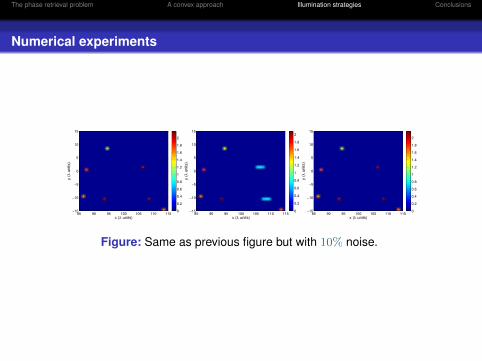
Figure: Same as previous figure but with 10% noise.

The phase retrieval problem A convex approach Illumination strategies Conclusions
Numerical experiments
x (λ units)
y (
λ u
nits)
85 90 95 100 105 110 115
15
10
5
0
−5
−10
−15
0.2
0.4
0.6
0.8
1
1.2
1.4
1.6
1.8
2
x (λ units)
y (
λ u
nits)
85 90 95 100 105 110 115
15
10
5
0
−5
−10
−15 0
0.1
0.2
0.3
0.4
0.5
0.6
0.7
0.8
x (λ units)
y (
λ u
nits)
85 90 95 100 105 110 115
15
10
5
0
−5
−10
−15 0
0.2
0.4
0.6
0.8
1
1.2
1.4
1.6
1.8
2
Figure: Same as previous figure but with 20% noise.

The phase retrieval problem A convex approach Illumination strategies Conclusions
Multiple frequency imaging
Imaging with M at a single frequency is not robust relative to smallperturbations in the unknown phases.
We can image robustly if wehave interferometric data (Borcea-Papanicolaou-Tsogka 05’,06’)
d((~xr, ~xr′), (~xs, ~xs′), (ω, ω′)) = P (~xr, ~xs;ω)P (~xr′ , ~xs′ ;ω
′) ,
and image interferometrically using
ICINT (~ys) =
∑~xs, ~xs′
|~xs − ~xs′ | ≤ Xd
∑~xr, ~xr′
|~xr − ~xr′ | ≤ Xd
∑ωl, ωl′
|ωl − ωl′ | ≤ Ωd
d((~xr, ~xr′ ), (~xs, ~xs′ ), (ωl, ωl′ ))
×G0(~xr, ~ys;ωl)G0(~xs, ~y
s;ωl)G0(~xr′ , ~ys;ωl′ )G0(~xs′ , ~y
s;ωl′ ).
Remark: Robustness comes at the cost of loss in resolution:λ0L/a→ λ0L/Xd in cross-range, and c0/B → c0/Ωd in range.

The phase retrieval problem A convex approach Illumination strategies Conclusions
Multiple frequency imaging
Imaging with M at a single frequency is not robust relative to smallperturbations in the unknown phases. We can image robustly if wehave interferometric data (Borcea-Papanicolaou-Tsogka 05’,06’)
d((~xr, ~xr′), (~xs, ~xs′), (ω, ω′)) = P (~xr, ~xs;ω)P (~xr′ , ~xs′ ;ω
′) ,
and image interferometrically using
ICINT (~ys) =
∑~xs, ~xs′
|~xs − ~xs′ | ≤ Xd
∑~xr, ~xr′
|~xr − ~xr′ | ≤ Xd
∑ωl, ωl′
|ωl − ωl′ | ≤ Ωd
d((~xr, ~xr′ ), (~xs, ~xs′ ), (ωl, ωl′ ))
×G0(~xr, ~ys;ωl)G0(~xs, ~y
s;ωl)G0(~xr′ , ~ys;ωl′ )G0(~xs′ , ~y
s;ωl′ ).
Or, restricting the data to a single receiver, using
ISRINT (~ys) =
∑~xs, ~xs′
|~xs − ~xs′ | ≤ Xd
∑ωl, ωl′
|ωl − ωl′ | ≤ Ωd
d((~xr, ~xr), (~xs, ~xs′ ), (ωl, ωl′ ))
×G0(~xr, ~ys;ωl)G0(~xs, ~y
s;ωl)G0(~xr, ~ys;ωl′ )G0(~xs′ , ~y
s;ωl′ ) .

The phase retrieval problem A convex approach Illumination strategies Conclusions
Numerical experiments: random medium
One realization of the random medium (correlation lengthl = 100λ0, strength of the fluctuations σ = 4 · 10−4).Measurements are for multiple frequencies covering a totalbandwidth of 120THz centered at f0 = 600 THz.Array size a = 500λ0 (0.25 mm) with N = 81 array elements, anddistance to the IW L = 10000λ0 (5mm depth).

The phase retrieval problem A convex approach Illumination strategies Conclusions
Weak random medium
The random fluctuations of the wave speed are modeled as
1
c2(x)=
1
c20
(1 + σµ(
x
l)
).
c0 denotes the average speedσ denotes the strength of the fluctuations with correlation length lµ(·) is a stationary random process with zero mean andnormalized autocorrelation function R(|x− x′|) = E(µ(x)µ(x′)),so that R(0) = 1, and
∫∞0R(r)r2dr <∞.
We use the random phase model which characterizes wavepropagation in the high-frequency regime in random media withweak fluctuations σ 1 and large correlation lengths l comparedto the wavelength λ.

The phase retrieval problem A convex approach Illumination strategies Conclusions
Imaging results random medium
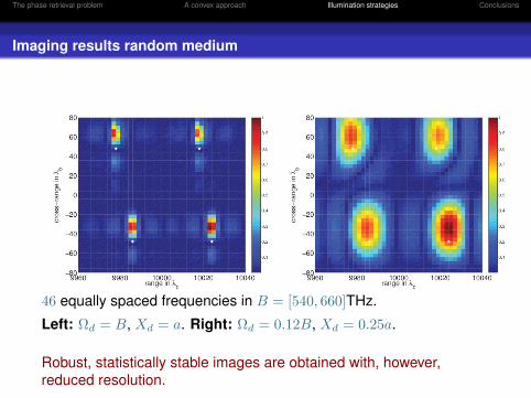
46 equally spaced frequencies in B = [540, 660]THz.
Left: Ωd = B, Xd = a. Right: Ωd = 0.12B, Xd = 0.25a.
Robust, statistically stable images are obtained with, however,reduced resolution.
The phase retrieval problem A convex approach Illumination strategies Conclusions
Imaging results random medium
46 equally spaced frequencies in B = [540, 660]THz.
Left: Ωd = B, Xd = a. Right: Ωd = 0.12B, Xd = 0.25a.
Robust, statistically stable images are obtained with, however,reduced resolution.

The phase retrieval problem A convex approach Illumination strategies Conclusions
Multiple frequency imaging
M. Moscoso, A. Novikov, G. Papanicolaou, and C. Tsogka,Multifrequency Interferometric Imaging with Intensity-OnlyMeasurements, SIAM Journal on Imaging Sciences 10 (2017).

The phase retrieval problem A convex approach Illumination strategies Conclusions
Statistical Stability
Reducing the data to nearby sources and nearby frequencies givesstatistically stability with respect to perturbations in the phases.
SRINT is equivalent to CINT for one receiver (which assumes phasesare recorded).
L. Borcea, G. Papanicolaou and C. Tsogka, Interferometric arrayimaging in clutter, Inverse Problems 21 (2005).
L. Borcea, G. Papanicolaou and C. Tsogka, Adaptiveinterferometric imaging in clutter and optimal illumination, InverseProblems 22 (2006).
L. Borcea, G. Papanicolaou and C. Tsogka., Coherentinterferometric imaging in clutter, Geophysics 71 (2006).
L. Borcea, J. Garnier, G. Papanicolaou and C. Tsogka, Enhancedstatistical stability in coherent interferometric imaging, InverseProblems 27 (2011).
The phase retrieval problem A convex approach Illumination strategies Conclusions
Concluding remarks
The convex approach guarantees exact recovery but it is notfeasible for large scale problems.Array imaging with intensities only in homogeneous media canbe as good as imaging with full information if we control theilluminations. Illumination diversity is the key.In weak random media, imaging with intensities-only using singlereceiver is stable. We use interferometric data somedium-induced phase perturbations cancel for nearbyfrequencies and illuminations.As a special case, we know how to recover exactly a vector fromthe absolute values of six versions of its DFT, in the imagingcontext, regardless of its size.

The phase retrieval problem A convex approach Illumination strategies Conclusions
Concluding remarks
Thanks!