Cluster Analysis of Spatial Patterns in Malaysian Tree Species

vol. 160, no. 5 the american naturalist november 2002

Cluster Analysis of Spatial Patterns in Malaysian Tree Species

Joshua B. Plotkin,1,2,* Jerome Chave,2 and Peter S. Ashton3

1. Institute for Advanced Study, Princeton, New Jersey 08540;2. Department of Ecology and Evolutionary Biology, PrincetonUniversity, Princeton, New Jersey 08544;3. Department of Organismal and Evolutionary Biology, HarvardUniversity, Cambridge, Massachusetts 02138

Submitted February 13, 2001; Accepted May 6, 2002

abstract: Tree species in tropical rain forests exhibit a rich panoplyof spatial patterns that beg ecological explanation. The analysis oftropical census data typically relies on spatial statistics, which quantifythe average aggregation tendency of a species. In this article wedevelop a cluster-based approach that complements traditional spa-tial statistics in the exploration and analysis of ecological hypothesesfor spatial pattern. We apply this technique to six study species withina fully mapped 50-ha forest census in peninsular Malaysia. For eachspecies we identify the scale(s) of spatial aggregation and the cor-responding tree clusters. We study the correlation between clusterlocations and abiotic variables such as topography. We find that thedistribution of cluster sizes exhibits equilibrium and nonequilibriumbehavior depending on species life history. The distribution of treediameters within clusters also varies according to species life history.At different spatial scales, we find evidence for both niche-based anddispersal-limited processes producing spatial pattern. Our method-ology for identifying scales of aggregation and clusters is general; wediscuss the method’s applicability to spatial problems outside of trop-ical plant ecology.

Subject heading: tropical forests, spatial statistics, spatial point pro-cesses, continuum percolation, dispersal limitation.

It has been firmly established that woody plant species andlianas exhibit spatial aggregation in natural communities.This trend has been especially well documented in species-rich communities, such as tropical rain forests, throughlarge-scale census experiments (Hubbell 1979; Hubbelland Foster 1983; He et al. 1997; Condit et al. 2000; Plotkinet al. 2000b). Although the primary cause of spatial pat-terns is hotly debated, the existence of spatial heterogeneityis fundamental to our theoretical and practical under-

* Corresponding author; e-mail: [email protected].

Am. Nat. 2002. Vol. 160, pp. 629–644. � 2002 by The University of Chicago.0003-0147/2002/16005-0008$15.00. All rights reserved.

standing of complex ecosystems (Ashton 1976, 1998; Hub-bell and Foster 1983; Hubbell 1997; Levin et al. 1997).The niche-based hypothesis attributes most species-levelheterogeneity to biotic and abiotic environmental varia-bility (Ashton 1969; Grubb 1977). However, even withouthabitat differentiation, neutral models of diversity predictthat dispersal limitation can itself account for the emer-gence of spatial clustering (Wong and Whitmore 1970;Hubbell 1997, 2001).

Why should tree species be spatially clumped? Why dothey not eventually occupy all suitable space evenly? Manyecologists (the niche theorists) argue that some sites are,at least at certain periods, unsuitable for certain species.This occurs because the species is not competitive in thelocal abiotic habitat, or pathogens or predators have elim-inated it locally (Janzen 1970; Connell 1971), or it is dueto some random vicissitude. Other ecologists (the neutraltheorists) contend that dispersal limitation and differentialmortality alone cause aggregated occupancy patterns.

Not until recently, however, with the advent of largebotanical inventories and long-term surveys, have thesefundamental issues been addressed with detailed empiricaldata. Methodologies for analysis of spatial data have be-come important for evaluating ecological theories. Suchanalyses usually employ the large body of spatial statisticsthat have been developed over the past century. Recentcontributions (He et al. 1997; Batista and McGuire 1998;Condit et al. 2000; Plotkin et al. 2000b) have quantifiedthe average clumping characteristics of tree species by util-izing a family of measures derived from the Ripley K sta-tistic (Ripley 1976). The K statistic computes the numberof conspecifics within a distance d from an individual,averaged over all individuals in the data set. To quantifyclumping, the observed K values are compared with thenull hypothesis of spatial randomness. Other commonmethodologies for analyzing spatial data include Fisher’squadrat-based variance-to-mean ratio (Fisher et al. 1922;David and Moore 1954; Lloyd 1967), nearest-neighbor sta-tistics (Pielou 1959; Pollard 1971; Diggle 1983; Cressie1991; He et al. 1997), and fitted spatial point processes(Diggle 1983; Cressie 1991; Batista and Maguire 1998; Plot-kin et al. 2000b).

In this article we address a generic limitation of such

630 The American Naturalist

statistical studies. Despite their broad efficacy, spatial sta-tistics essentially quantify the average aggregation patternof a species. This limitation often has induced ecologiststo assign a single scale of aggregation to each species (Con-dit et al. 2000; Plotkin et al. 2000b, He and Gaston 2000)even though a species can be aggregated at several scalessimultaneously. Many ecological questions, such as theinfluence of habitat differentiation, can be better addressedby identifying the specific position, size, and shape of thespatial clusters in a data set. This task is tantamount topartitioning survey data into distinct clusters.

The problem of partitioning data has been investigatedextensively in many disciplines (Duda et al. 1998). In thisarticle we develop an approach to identifying clusters inspatial data, at several spatial scales, without making anya priori assumptions on the structure of clusters. We applythis technique to a 50-ha permanent sampling plot of trop-ical rain forest. Using select species from the 50-ha survey,we investigate the potential effects of habitat differentiationand dispersal limitation, that is, niche-based and dispersal-based hypotheses, on the spatial arrangement of individ-uals at various spatial scales. For each species we identifythe scale(s) of spatial aggregation and the correspondingtree clusters. We study the correlation between cluster lo-cations and abiotic variables such as topography, the dis-tribution of cluster sizes, and the distribution of tree di-ameters within clusters. We conclude by discussing therelative merits of our cluster-based approach and spatialstatistics in general.

Material and Methods

Study Site

The Pasoh Forest Reserve, Negiri Sembilan, Malaysia, is a2,450-ha protected forest of the Keruing-Meranti type. Itsflora has been studied since 1970 (Wong and Whitmore1970; Ashton 1976; P. S. Ashton, unpublished manuscript,1971). The canopy of the Pasoh forest is dominated bydipterocarp trees, mostly in the genera Shorea, Diptero-carpus, and Neobalanocarpus. Mean rainfall at the studysite is relatively low, approximately 2,000 mm/yr, but with-out marked seasonality.

A 50-ha permanent sampling plot was established in1987 by the Forest Research Institute of Malaysia to mon-itor long-term changes in primary forest (Manokaran andKochummen 1987; Kochummen et al. 1990; Manokaranand LaFrankie 1990). The Pasoh plot, located at 102�18�Wand 2�55�N, is a rectangular census 1 km long and 0.5 kmwide. The plot’s topography is fairly even, with a gentleslope rising 24 m toward the northwest. There are twoprimary streams within the plot. All 335,256 free-standingwoody stems exceeding 1 cm diameter at breast height

(dbh) were identified to species and spatially mapped to!1 m accuracy (see Manokaran and LaFrankie 1990),yielding 816 species, 294 genera, and 74 families. The ini-tial census of 1987 has been repeated in 1990 and 1996.The 1996 data are used throughout this article. The Pasohplot is part of a long-term research program worldwide,coordinated by the Smithsonian’s Center for Tropical For-est Science.

We have selected this plot because it has motivated sev-eral statistical studies in the past few years (He et al. 1997;Condit et al. 2000; Plotkin et al. 2000a, 2000b; He andGaston 2000). Hence, our cluster analysis may be easilycompared with prior results of a more statistical nature.

Study Species

Previous studies of spatial pattern in tropical forests (Heet al. 1997; Condit et al. 2000; Plotkin et al. 2000b) haveaddressed the question of how many species are aggre-gated. These studies have clearly concluded that most spe-cies are clumped, and a few are randomly distributed. Thisconclusion was based on spatial statistics, which are oftendeficient for rare species.

Here, by contrast to previous studies, we focus on ahandful of carefully chosen species. We have selected fourabundant and two rare species in the Pasoh permanentplot. Xerospermum noronhianum (Blume) Blume Sapin-daceae is a subcanopy species and the most common inthe plot (8,820 stems, average dbh cm, maximalD p 3.19dbh cm). It is recorded as a peat swamp forestD p 37.3max

specialist. It is abundant in mesic moist sites throughoutwestern Malaysia but also is widespread in other lowlandhabitats in mixed dipterocarp forest. The seeds of X. no-ronhianum are dispersed by the monkey, the crab-eatingor long-tailed macaque, and by the gibbon (Yap 1976).Knema laurina (Blume) Warb. Myristicaceae (4,088 stems,

cm, cm) is a subcanopy speciesD p 2.53 D p 35.4max

often found on sand or clay.Neobalanocarpus heimii (3,334 stems, cm,D p 5.0

cm) is an emergent dipterocarp and a com-D p 196.8max

mercial timber known as chengal. It is endemic to pen-insular Malaysia and is widespread there on sandy allu-vium and on ridges to about 1,000 m. It is sometimesgregarious. It is shade tolerant as a juvenile and has veryhard durable wood (specific density 0.7–0.8 g/cm3). Withlarge wingless fruit, the seed has no known means of dis-persal. Neobalanocarpus heimii is the ultimate climax spe-cies, able to regenerate even in very small light gaps.

Shorea macroptera (1,508 stems, cm,D p 6.1 D pmax

cm) is a main-canopy dipterocarp and a leading102.5species in the so-called Red Meranti–Keruing type ofmixed dipterocarp forest on suitable soils throughout west-ern Malaysia. The fruit bears slightly twisted, aliform, ex-

Cluster Analysis of Malay Trees 631

Figure 1: Schematic spatial arrangement of six data points in the plane.Points within a radius d are assigned to the same cluster; hence, pointsa, b, c, and d are in the same cluster. Points e and f are in separate clusters.

panded sepals, so that it is dispersed by gyration and some-times wind. It is also a light demander and regeneratesfrom established seedlings after the formation of largegaps. Shorea macroptera follows life-historical strategiesthat are extremely different from those of N. heimii.

In addition, we have studied two less abundant specieswith peculiar spatial patterns. Mallotus penangensis Muell.Arg. Euphorbiaceae (1,404 stems, cm,D p 4.56 D pmax

cm) is a subcanopy tree found on various habitats both24in peninsular Malaysia and in Borneo (known as Mallotussarawacensis). Pternandra coerulescens Jack Melastomata-ceae (438 stems, cm, cm) is a sub-D p 5.31 D p 25max

canopy species found mainly along watercourses or wher-ever ground litter is minimal.

Clustering Spatial Data

Algorithm Specification

We present a technique of spatial analysis that identifiesthe location of intraspecific tree clusters in a fully censusedforest plot. This technique will serve as the basis for an-alyzing the spatial patterns of our six study species. Treelocations are henceforth considered as punctual. Our tech-nical problem is, therefore, to define and detect the spatialclusters for a set of points in the plane. In addition, wewish to detect “critical distances” or “critical scales” relatedto the observed data. When data contain more than onecritical distance, classical statistics would yield an averageof these distances and, thus, a fairly imprecise character-ization. The most straightforward method for partitioningdata into clusters is by visual inspection. However, thismethod is subjective and time consuming. We desire arigorous technique of cluster detection that requires no apriori assumptions about the shape of the clusters. We alsowant to detect clusters even if they are not radially sym-metric or approximately symmetric. We now present anefficient technique for addressing both questions.

We say that two trees are connected if their stems areseparated by a distance d or less. Two trees are said tobelong to the same cluster if they are related by a path ofconnected trees. For example, if tree A is connected totree A, and tree B is connected to tree C, then all threetrees will belong to same cluster, even if A and C are notdirectly connected. This definition of a cluster, illustratedgraphically in figure 1, is extremely simple and natural. Inaddition, this definition allows us to interpret cluster anal-ysis in the language of statistical mechanics (see “Perco-lation and Critical Distances”).

Given a value of the clustering distance d, our algorithmpartitions the data into distinct spatial clusters. The dis-tance d is a free parameter of the algorithm. Once d is

specified, there is a unique corresponding partition of thedata into disjoint clusters. In the trivial case when d p

, each tree forms its own distinct cluster, but when d is0very large (larger than the maximal pairwise distance be-tween two trees), there is only one cluster; all trees arepairwise connected. Interesting patterns emerge for inter-mediate values of the clustering parameter d. The appendixdescribes an efficient implementation of our algorithm aswell as some related subtleties of its execution.

Percolation and Critical Distances

Spatial statistics typically are compared against the nullmodel of randomly distributed points. In order to gainsome intuition about our clustering algorithm, we tem-porarily restrict our focus to the case of random datapoints. An understanding of this scenario will improve ourinterpretation of the cluster results in the forthcomingapplied setting. When data are random, the behavior ofour algorithm is, in fact, equivalent to the “continuumpercolation problem,” a well-researched topic in statisticalphysics (Broadbent and Hammersley 1957; Stauffer andAharony 1994). The partitions identified by our algorithmundergo a sharp transition as the parameter d increases.Before the transition, most data points are isolated; afterthe transition, most points belong to the same large cluster.This phenomenon is known as the “percolation transi-tion.” Percolation is usually studied when data points are


Figure 2: a, Idealized relationship between the distance parameter d andthe mean cluster size. A sharp (critical) transition is predicted at a singledistance dc if the data points are randomly distributed in space and ifthe sample size is large. As d passes through the percolation thresholddc, the data points become connected in space and the mean cluster sizeundergoes a phase transition from 0 to 1. b, Influence of finite samplesize on the “continuum percolation” transition. The transition occurs atthe same critical distance as in the large sample size limit (a), but thetransition is not as sharp. c, Percolation behavior for simulated data. Ineach of the four data sets, points have been placed in space at randomwith density 0.1. The largest data set contains points, andn p 12,500

the smallest data set, points. As the sample size gets smaller,n p 100the transition becomes more gradual, as depicted schematically in a. Seethe appendix for a discussion of minimizing sample size artifacts.

constrained to remain on a discrete lattice (see, e.g., Keittet al. 1997; and Keymer et al. 2000 for applications inecology). In our case, however, tree locations are uncon-strained, and the corresponding process is called “contin-uum percolation” (Hall 1985; Meester and Roy 1996).

As we vary the cluster parameter d, we obtain corre-sponding partitions of the data into disjoint clusters. Forany given d value, we denote the number of resultingclusters by m and the size of the clusters by

. Let denote the total number ofc , c , … , c n p � c1 2 m i

individuals in the sample. We can conveniently summarizea cluster arrangement by recording the mean cluster size,that is, the first moment of the cluster size distribution:

m mc 1i 2AcS p # c p c .� �i in nip1 ip1

The mean cluster size equals the expected size of the clustercontaining a randomly chosen individual. The normalizedmean cluster size, , computes the probability that twoAcS/nrandomly chosen data points lie in the same cluster.

Percolation theory predicts that below a certain criticaldistance, dc, individuals will be distributed in many smallclusters, while above this distance most individuals willbelong to a single large cluster. The critical distance dc atwhich the clusters undergo this transition is called the“percolation threshold.” The transition will be increasinglysharp as number of individuals in the data sample in-creases. The percolation transition may also be stated interms of the mean cluster size: the (normalized) meancluster size of a very large random data set will equal 0below the critical distance dc and 1 above the critical dis-tance. Figure 2 demonstrates the percolation transition bygraphing the distance parameter d against the mean clustersize for a simulated set of random data points.AcS

In real data, as opposed to random data, we do notexpect to find a single sharp transition at one critical dis-tance. Instead, we may often discover several critical dis-tances with varying degrees of sharpness. Such behavioris indicative of spatial clustering at several scales. As wevary the distance parameter d, producing different parti-tions of the data into clusters, we will detect critical dis-tances by graphing d against the corresponding mean clus-ter size . Any range of distances d that corresponds toAcSa plateau in the cluster size curve indicates a nonrandomscale of aggregation that is insensitive to perturbations ind. In general, the number of plateaus in the observed


cluster size curve will reflect the number of nonrandomscales of aggregation.

In order to compare cluster behavior across species withdifferent abundances, we must normalize the distance pa-rameter d. We will divide d by the quantity

1 �A/n,2

which is the average nearest-neighbor distance for n ran-domly placed data points. The normalized parameter isdenoted

ˆ �d p 2d n/A.

Here A denotes the total sample area, and n denotes theabundance of the species. This normalization produces anondimensional version of cluster parameter , suitabledfor interspecific comparison. In the limit of a large samplesize and a random data set, the sharp transition will occuraround , regardless of the density of points.d ≈ 2.4

Techniques for the Study of Habitat Associations

The association of species with habitat type was one ofthe first questions studied by tropical botanists (see, e.g.,Richards 1936). This question was a primary motivationfor many large-scale studies in Southeast Asia (Ashton1964) and in the Neotropics (Gentry 1988). Such studieshave stimulated the development of statistical methods fordetecting “phytosociological units” or habitat associations.

In essence, statistical methods of habitat correlationquery, with varying degrees of sophistication, whether ornot a species is overrepresented in a particular habitat; x2

(Basnet 1992) and modified x2 (e.g., Harms 1996; Plotkinet al. 2000b) tests are the most common statistical analyses.Such techniques are undeniably useful in quantifying over-all patterns of habitat associations. Yet their ability to char-acterize the specific effects of habitat on any particularspecies is modest: such tests simply inform us whether ornot a species is associated (positively or negatively) witha given habitat. Moreover, such tests are only possible ifcomplete and consistent abiotic measurements have beenperformed throughout the survey area. We will demon-strate how cluster analyses can complement existing sta-tistical techniques. Cluster analysis can elucidate habitatassociations for rare and common species alike, even insituations where more classical statistical analyses fail todetect or to characterize associations. The dual informa-tion of the location and the shape of a cluster is extremelyuseful in assessing potential habitat specializations.

Results

Identification of Spatial Clumps

As a preliminary example of our cluster algorithm, we firstconsider Mallotus penangensis, a species with a noniso-tropic spatial distribution. Figure 3 shows the primaryoutput of our algorithm. Cluster analyses are shown fortwo distances, m and m (fig. 3a). Fig-d p 12.4 d p 20.8ure 3b shows the relationship between the normalized clus-ter parameter and the corresponding mean cluster size.dNotice that the cluster behavior summarized in figure 3bis very different from the random case discussed above(fig. 2c). Instead of a single percolation threshold at d ≈

, M. penangensis displays two transitions occurring at2.4approximately 1.5 and 8.0. The first transition occurs ata smaller distance than for random data and the second,at a much larger distance. The distance required to connectall points into a single cluster is much larger for the Mal-lotus data ( ) than for the random data ( ).ˆ ˆd 1 8 d p 3

The M. penangensis clusters undergo their first transitionat , and the mean cluster size remains fairly con-d ≈ 1.5stant on a plateau for a range of distances thereafter (fig.3b). This indicates that the M. penangensis clusters are welldefined over a large range of scales ( ). Theˆ1.5 ! d ! 6.0two d values chosen in figure 3a correspond to d p 1.3and ; these two values demonstrate the clusterd p 2.2structure before and after the first transition. Figure 3bindicates that the right panel of figure 3a is a better clus-tering of the M. penangensis species than the left panel, inthe sense that the clusters are robust to perturbation.

The precise relationship between cluster structure anddistance parameter is best summarized by the graph infigure 3b. Nevertheless, figure 4 provides an alternative,three-dimensional summary of this relationship. The Z-axis of figure 4 corresponds to the distance parameter d.For convenience, clusters are represented schematically bycircles (in fact, clusters are not symmetric). The top layer,

, shows the locations of every tree in green. On thez p 0bottom layer ( m) all the trees are within the samed p 134large cluster, represented by a single circle. As d increasesdown the Z-axis, the number of clusters decreases and thecluster sizes increase. The critical transitions in this spec-trum are visible in figure 4, but they are perhaps discernedmore accurately by graphing the mean cluster size (fig.3b).

Our analysis of M. penangensis highlights two importantregimes of spatial patterns: stable regions in which theclusters are well defined and sensitive regions in which thecluster structure undergoes dramatic transitions. Depend-ing on the ecological question at hand, either one of theseregimes may be of interest. In the case of M. penangensis,the stable region most likely indicates the clustering thatcorresponds to dispersal-driven clumps of related trees. As


Figure 3: a, Cluster analysis of the understory species Mallotus penangensis, Euphorbiaceae. There are 1,404 stems of this species in the Pasoh 50-ha plot. When we set the clustering distance d equal to 12.4 m, the algorithm partitions the data into 75 distinct clusters, each plotted in a differentcolor (left panel). Some colors may appear similar. Setting m results in 34 clusters (right panel). b, Mean cluster size as a function of thed p 20.8normalized distance parameter for M. penangensis. The algorithm was run with a temperature to minimize finite-size artifacts (see appendixx p 0.08for details).

we shall see, however, the critical regimes can also be usefulfor detecting the influences of habitat.

Habitat Associations

Pternandra coerulescens. The species P. coerulescens pro-vides an instructive comparison with M. penangensis. Bothspecies demonstrate essentially two critical distances (figs.3b, 5b). For P. coerulescens, the transitions occur at d ≈

and . The clusters of P. coerulescens shown inˆ1.2 d ≈ 2.5figure 5a occur in the stable region immediately after the

first critical distance. Unlike M. penangensis, the clustersof P. coerulescens are long, narrow, and linear in shape,with a few exceptions. Notice that both cluster geometriesare simultaneously detected by our algorithm. Pternandracoerulescens also features a large number of singleton treeslocated far away from conspecifics. This feature, seengraphically in figure 5a, is reflected by the long tail of thecluster size curve in figure 5b. The tail is caused by thegradual assimilation of singleton trees into the main clusterat large distances d.

Pternandra coerulescens exhibits clusters with a verycharacteristic shape. The hypothesis that P. coerulescens is


Figure 4: Dependence of clusters on the distance parameter d for Mallotus penangensis. The figure shows a three-dimensional graph of M. penangensisclusters. The X- and Y-axes of the figure correspond to the length and width of the 50-ha plot, as in figure 3a. The Z-axis corresponds to the valueof d. The color also corresponds to the value of d. On the upper plane, , and each tree forms its own cluster, all plotted in green. As dd p 0increases down the Z-axis, larger clusters form. Each cluster is represented in the figure by a circle centered at the center of mass of the cluster.The radius of the circle equals the mean distance of the trees in the cluster to its center of mass.

associated with local streams, which stands out as the mostnatural in light of figure 5b, is confirmed by the naturalhistory of the species (see “Study Species”). This suggeststhat the linear-shaped clusters are the direct result of P.coerulescens’s finicky habitat requirements. Indeed, P. coe-rulescens mainly grows wherever ground litter is minimalor absent. The latter observation was made during a trop-ical plant biomass experiment in 1971–1973 when all free-standing trees and litter were removed from a survey plotnear Pasoh’s 50-ha plot (Kira 1971). Pternandra coerules-cens, normally a fairly rare species, colonized most of thelogged region, presumably due to the complete absence ofground litter there (T. Kira, personal communication). Inaddition, P. coerulescens also clusters at the primary pigwallows in the plot (fig. 5a), another location with frequentlitter disturbance. Despite the numerous, widespread,

small seeds produced by P. coerulescens, the species is se-verely limited by abiotic environmental factors. Since mapsof Pasoh’s local stream networks (and many other abioticenvironmental variables) are not available, the presentanalysis would have been much more difficult, or impos-sible, via classical tests of habitat specificity.

Xerospermum noronhianum and Knema laurina. We turnnow to the environmental influences on two of the mostcommon Pasoh species: Xerospermum noronhianum andKnema laurina. In particular, we examine the effect oftopography of their spatial distributions. A Ripley K anal-ysis indicates that both of these species follow nonrandomspatial distributions (Plotkin et al. 2000b). The cause ornature of the nonrandomness is difficult to determine withthe naked eye. Statistical tests indicate that neither of these


Figure 5: a, Cluster analysis of Pternandra coerulescens that results fromthe distance parameter m ( ). There are 438 stems withinˆd p 25.4 d p 1.5the plot, which form 79 clusters. Most of the clusters of P. coerulescensare linear in shape. The arrow indicates the locations of pig wallowswithin the 50-ha plot. b, Mean cluster size curve for P. coerulescens. Thealgorithm was run with a positive temperature ( ) to minimizex p 0.08finite size effects. The resulting curve shows two principal transitions.

Figure 6: a, Topographic contour map of the Pasoh 50-ha plot. Theprimary water drainage route running off the hill is indicated in red. b,Cluster analysis of Knema laurina for m (330 disjoint clusters).d p 12.1Notice that K. laurina forms a single, stable cluster on the hill. c, Clusteranalysis of Xerospermum noronhianum for m (494 disjoint clus-d p 9.0ters). Notice that X. noronhianum tends to form larger, stable clustersoff of the hill. The water drainage route apparently disrupts the X. no-ronhianum clusters. See figure 7 for the relationship between distanceparameter d and mean cluster size.

species is very strongly correlated with Pasoh’s topography(Plotkin et al. 2000b). In particular, for each species, thetotal density of stems on the hill is roughly equal to thedensity of stems off the hill. Although topography doesnot limit the ranges of these species, it might, nevertheless,influence the spatial geometry of individual treeplacement.

Figure 6b shows that topography does have an effect onthe spatial distribution of these two species, despite theabsence of a strong statistical correlation with topography.Knema laurina exhibits one large cluster whose boundariesclearly coincide with the detailed topography of the single


Figure 7: Mean cluster size curve for Xerospermum noronhianum. Thealgorithm was run with a positive temperature, (see appendixx p 0.05for details). The critical value yields the cluster arrangementd p 2.4displayed in figure 6c. The mean cluster size curve for Knema laurina(not shown) is very similar.

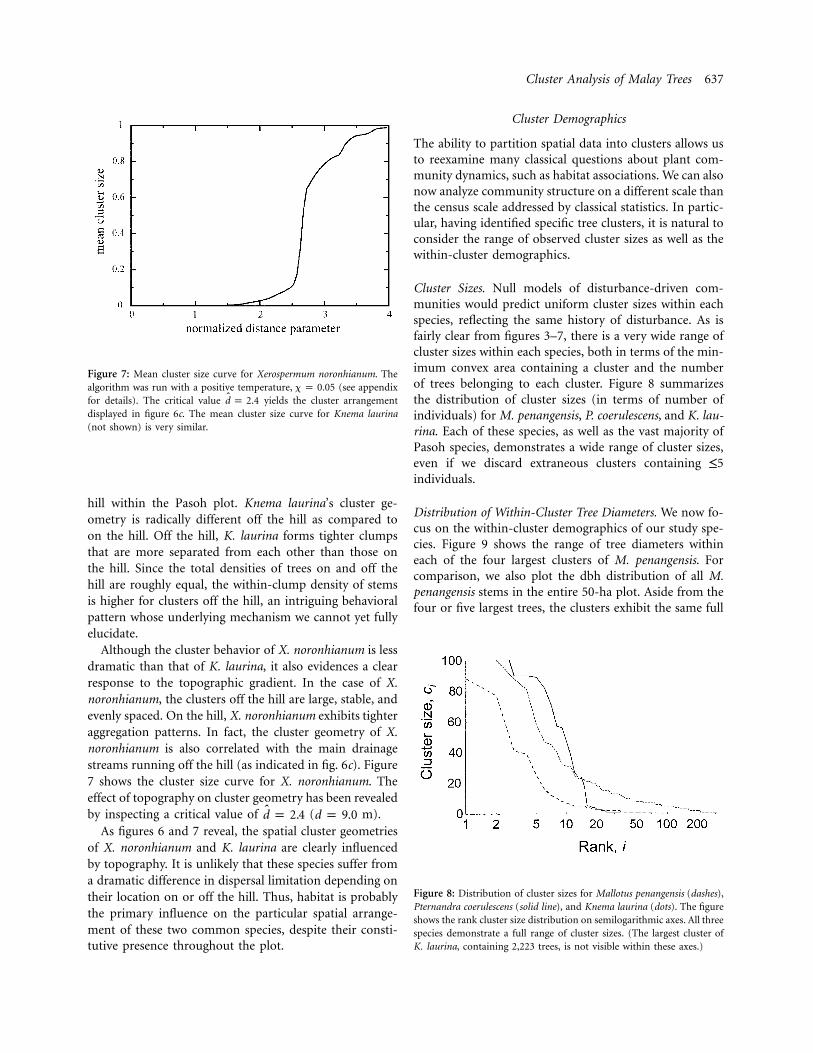
Figure 8: Distribution of cluster sizes for Mallotus penangensis (dashes),Pternandra coerulescens (solid line), and Knema laurina (dots). The figureshows the rank cluster size distribution on semilogarithmic axes. All threespecies demonstrate a full range of cluster sizes. (The largest cluster ofK. laurina, containing 2,223 trees, is not visible within these axes.)

hill within the Pasoh plot. Knema laurina’s cluster ge-ometry is radically different off the hill as compared toon the hill. Off the hill, K. laurina forms tighter clumpsthat are more separated from each other than those onthe hill. Since the total densities of trees on and off thehill are roughly equal, the within-clump density of stemsis higher for clusters off the hill, an intriguing behavioralpattern whose underlying mechanism we cannot yet fullyelucidate.

Although the cluster behavior of X. noronhianum is lessdramatic than that of K. laurina, it also evidences a clearresponse to the topographic gradient. In the case of X.noronhianum, the clusters off the hill are large, stable, andevenly spaced. On the hill, X. noronhianum exhibits tighteraggregation patterns. In fact, the cluster geometry of X.noronhianum is also correlated with the main drainagestreams running off the hill (as indicated in fig. 6c). Figure7 shows the cluster size curve for X. noronhianum. Theeffect of topography on cluster geometry has been revealedby inspecting a critical value of ( m).d p 2.4 d p 9.0

As figures 6 and 7 reveal, the spatial cluster geometriesof X. noronhianum and K. laurina are clearly influencedby topography. It is unlikely that these species suffer froma dramatic difference in dispersal limitation depending ontheir location on or off the hill. Thus, habitat is probablythe primary influence on the particular spatial arrange-ment of these two common species, despite their consti-tutive presence throughout the plot.

Cluster Demographics

The ability to partition spatial data into clusters allows usto reexamine many classical questions about plant com-munity dynamics, such as habitat associations. We can alsonow analyze community structure on a different scale thanthe census scale addressed by classical statistics. In partic-ular, having identified specific tree clusters, it is natural toconsider the range of observed cluster sizes as well as thewithin-cluster demographics.

Cluster Sizes. Null models of disturbance-driven com-munities would predict uniform cluster sizes within eachspecies, reflecting the same history of disturbance. As isfairly clear from figures 3–7, there is a very wide range ofcluster sizes within each species, both in terms of the min-imum convex area containing a cluster and the numberof trees belonging to each cluster. Figure 8 summarizesthe distribution of cluster sizes (in terms of number ofindividuals) for M. penangensis, P. coerulescens, and K. lau-rina. Each of these species, as well as the vast majority ofPasoh species, demonstrates a wide range of cluster sizes,even if we discard extraneous clusters containing ≤5individuals.

Distribution of Within-Cluster Tree Diameters. We now fo-cus on the within-cluster demographics of our study spe-cies. Figure 9 shows the range of tree diameters withineach of the four largest clusters of M. penangensis. Forcomparison, we also plot the dbh distribution of all M.penangensis stems in the entire 50-ha plot. Aside from thefour or five largest trees, the clusters exhibit the same full


Figure 9: Distribution of tree diameters within the four largest Mallotuspenangensis clusters, compared with the distribution of M. penangensisdiameters in the entire 50-ha census (large dots). The figure shows a rankdbh plot on a semilogarithmic axis. The individual clusters of M. pen-angensis exhibit nearly the same full range of dbh classes as the 50-haplot as a whole.

range of diameters as the 50-ha census taken altogether.Moreover, the dbh distribution is approximately expo-nential at both the cluster scale and the full 50-ha scale.These results indicate that the identified clusters of M.penangensis represent full-fledged microcommunities oftrees, containing juvenile and mature stems alike. We donot find any examples of purely juvenile or purely adulttrees, which would be obvious signatures of a system awayfrom equilibrium. Instead, the clusters of M. penangensisare in equilibrium, in that we do not expect their diameterdistribution to change significantly in time.

A full range of intracluster diameters is common amongthose Pasoh species that demonstrate obvious aggregationpatterns. The trend demonstrated by M. penangensis alsoholds for our other study species. Species Neobalanocarpusheimii is a rare counterexample: its large clusters dem-onstrate an elevated proportion of juveniles, comparedwith the dbh distribution in the plot as a whole. Theunusual nonequilibrium distribution of N. heimii reflectsits characteristic ability to regenerate quickly in small gaps.

Cluster Structure and Tree Diameters. In addition to therange of within-cluster tree diameters, we are also inter-ested, naturally, in the relative locations of large and smalltrees within a cluster. In particular, are clusters character-ized by one or several large “mother trees” located nearthe cluster center? Or are large trees more often found onthe periphery of clusters? Such questions are relevant toan understanding of those processes behind clusterformation.

We have found examples of both trends within the Pa-soh plot. Many species exhibit random within-cluster treeplacement, with respect to tree diameter. Many other spe-cies exhibit an elevated proportion of large peripheraltrees. And only a few species exhibit large central trees.This finding, which we document in two particular in-stances below, may be somewhat surprising compared withthe simplistic view of a dispersal-driven cluster with centrallarge “mother trees.” Shorea macroptera exhibits an ele-vated proportion of peripherally located large trees. Figure10a shows a cluster analysis of S. macroptera in which thesize of each circle corresponds to the tree’s diameter. It isnot immediately apparent to the eye whether large treesare central or peripheral. With the explicit knowledge ofthe cluster partition, however, we can test for statisticalcorrelations between tree diameter and within-clusterplacement.

We define the center of a cluster to be the average Xand Y coordinate of all those trees in the cluster. Thisdefinition assumes some degree of isotropy. For each clus-ter, we inspect the relationship between a tree’s dbh andits distance to the center of its cluster. We normalize thisdistance by dividing by the mean distance to the centeramong all trees in the cluster. Finally, we calculate thePearson’s correlation coefficient of the relationship be-tween dbh and distance to center for each cluster.

The correlation between tree diameter and distance tocenter is shown for each cluster of S. macroptera in figure10b. Notice that most of the large clusters demonstrate apositive correlation. Pooling the dbh distance data fromthe 10 largest clusters of S. macroptera together, the positivecorrelation between dbh and distance is statistically sig-nificant at the 95% confidence level: larger trees tend tolie on the periphery of their cluster. The same finding holdsfor many other Pasoh species, including, for example, Dip-terocarpus cornutus, Shorea guiso, Schoutenia accrescens,and Eugenia claviflora.

Figure 11 demonstrates a parallel analysis for N. heimii.In this case, however, the large clusters demonstrate a neg-ative correlation between dbh and distance to cluster cen-ter. Pooling the data from the 10 largest clusters together,there is again a statistically significant result at the 95%level: larger trees tend to be found closer to the center ofthe cluster. Among the Pasoh species, N. heimii is a some-what rare example of this central large tree phenomenon.The tendency for large trees to be located in the center ofclusters, as opposed to the periphery, is indicative of strongintraspecific competition. Despite an abundant seed rainaround many large, reproductive, locally dispersed trees,seedlings have difficulty establishing themselves in thenearby vicinity of large conspecifics and find themselvesmarginalized on the periphery. Most of this intraspecificcompetition occurs before stems reach 1 cm diameter


Figure 10: a, Cluster analysis of Shorea macroptera corresponding to, resulting in 171 clusters. The radius of each circle representsd p 1.4

the diameter of the corresponding tree, although not to scale. b, Pearsoncorrelation coefficient for the within-cluster relationship between dbhand distance to cluster center for all S. macroptera clusters. The X-axisdenotes the size of the cluster, and the Y-axis denotes the correlationcoefficient for the trees within the cluster. Notice that most of the largeclusters exhibit a positive correlation between dbh and distance to center;large S. macroptera trees are found toward the periphery of their cluster.

Figure 11: a, Analysis of Neobalanocarpus heimii parallel to figure 10.The cluster algorithm was run at , resulting in 1,200 clusters. b,d p 1.1Pearson correlation coefficient for the within-cluster relationship betweendbh and distance to cluster center for all N. heimii clusters. Notice thatmost of the large clusters exhibit a negative correlation between dbh anddistance to center. In other words, large trees of N. heimii are found nearthe center of their cluster.

(Wills and Condit 1999). Thus, within-cluster demograph-ics may be a strong indicator of intraspecific forces andeven Janzen-Connell effects (Janzen 1970; Connell 1971).

It is interesting to note that N. heimii and S. macropterahave radically different dispersal mechanisms (see “StudySpecies”). The dispersal differences between these two dip-terocarps are clearly correlated with the different spatialpopulation structures of their clusters (fig. 10 vs. fig. 11).Such an observation would perhaps be predicted from anunderstanding of life-history traits and from visual in-spection but can only be verified rigorously by a completecluster analysis. In the case of N. heimii, trees that succeedto maturity then escape competition and continue to live

reproductively for centuries. Because of their large winglessfruit, most juveniles do not survive the stifling dark pa-rental subcanopy light climate. As a result, there are severallarge central stems of N. heimii surrounded by a range ofaspiring juveniles on the perimeter, most of which will notsurvive. This interpretation agrees with our earlier obser-vation of an elevated proportion of juveniles found inclusters of N. heimii.

The seeds of S. macroptera, by contrast, are well dis-persed, and the growth rates are also higher. Moreover,adult stems of S. macroptera do not persist as long as N.heimii. As a result, old clumps of S. macroptera may havenew clumps growing in gaps and around their perimeters;we therefore find a positive correlation between dbh anddistance to center.

It is also interesting to compare the cluster demograph-


ics of N. heimii with those of the ballistically dispersed M.penangensis. On the face of it, these two species might beexpected to demonstrate similar within-cluster spatialstructure. However, M. penangensis does not, in fact, ex-hibit any significant correlation (positive or negative) be-tween distance and size, in contrast to N. heimii’s negativecorrelation. This observation likely reflects the fact that N.heimii does not reproduce until its crown has emergedabove the canopy, perhaps after at least 50 yr. Mallotuspenangensis, which also is a slow grower, nevertheless startsreproducing when quite small, so that a range of sizes aredispersing seeds within the cluster, resulting in no con-sistent space-diameter correlations.

In summary, we have seen that there is a large range ofcluster sizes within each species and that clusters generallyexhibit a full range of tree sizes, whose distribution issimilar to the dbh distribution found in the 50-ha plot asa whole. In addition, many species exhibit large trees onthe periphery of their clusters, few species exhibit clusterscentered around large trees, and many species exhibit noconsistent spatial size class structure. And finally, many ofthese trends reflect the different dispersal mechanisms andgrowth patterns between species.

Discussion

Ecological Implications

Ecologists address questions of community dynamics onmany spatial scales: individuals, censuses, regions, andlandscapes. Once spatial data have been partitioned intoclusters, however, we can inspect community dynamics ontwo new scales: the intracluster and intercluster scales. Inour case, clustering has allowed us to examine several is-sues of importance in tropical plant ecology: the corre-lation between cluster locations and abiotic environmentalvariables, the distribution of cluster sizes, the distributionand spatial placement of within-cluster tree diameters.

This technique has allowed us to unveil hidden patterns(for Xerospermum noronhianum and Knema laurina)whose discovery might otherwise have been impossible.Such discoveries suggest that habitat may have a strongereffect on the spatial distribution of common species—evenspecies that are present constitutively on all habitattypes—than standard statistical analyses would suggest. Inaddition, cluster analysis of species such as Pternandracoerulescens demonstrate that spatial distribution cansometimes be driven almost entirely by abiotic habitatspecificity, regardless of dispersal capability.

At the same time, our investigation of cluster demo-graphics has revealed that dispersal mechanisms and

growth patterns can play a large role in determining in-tracluster spatial population structure. Species-level vari-ation in regeneration speed is reflected by variation in therange of tree diameters found within clusters. Gap colo-nizers (e.g., Neobalanocarpus heimii) may be identified,from static data alone, by a signature elevated proportionof purely juvenile clusters. Differences in dispersal mech-anism (e.g., Shorea macroptera vs. N. heimii) are associatedwith characteristic differences in the placement of largetrees within a cluster. Similarly, differences in growth pat-terns (e.g., Mallotus penangensis vs. N. heimii) are alsoreflected by within-cluster tree placement; species that re-produce throughout their lifetime may lack any correlationbetween diameter and intracluster placement.

In short, we have found that the diversity of tropicaltree life-historical traits and of the diversity of responsesto abiotic influences are reflected by the diversity of theirspatial arrangements. Thus our study species evidence bothniche-based and dispersal-based processes affecting spatialdistributions, at different spatial scales.

We emphasize that, despite the analysis of our studyspecies, our cluster method does not allow us to inferprocess unambiguously from pattern. We cannot soundlyargue to have teased apart the influences of niche- anddispersal-based processes in general. In the end, we viewthe techniques developed here more as tools for explor-atory data analysis and for generating hypotheses. Suchhypotheses (e.g., the disequilibrium dynamics of N. heimii)must eventually be tested by field and lab experiments.Nevertheless, we have seen that careful direct observationof species’ maps can, when combined with a clusteringalgorithm, provide a powerful method for ecologicalexploration.

Cluster Analysis and Spatial Statistics

We have developed a fairly general method for analyzingspatial distributions that is conceptually different from theclassical paradigm of spatial statistics. Spatial statistics havebeen used to assess mean clumping behavior across theentire range of species in order to document universaltrends of aggregation in forests. The cluster techniquesdeveloped here complement such gross statistics.

One might argue that a formal clustering technique pro-vides little more information than an automated mappingdevice. The human eye is, in fact, a remarkably efficientand complex tool for detecting spatial patterns. The meth-odology developed here, however, permits us to reframespecific questions of tree dynamics in terms of spatial scalesand to identify the relevant critical scale(s) for a givenspecies. Several critical scales indicate multiple factors thatinfluence a species’ distribution. There is no single “correct


answer” to partitioning spatial data but, rather, a spectrumof answers among which our method guides us towardthe critical and stable solutions.

Unlike most spatial statistics, our method of identifyingclusters does not make a priori assumptions about un-derlying spatial structure. The edge-correction factors usedto compute spatial statistics, by contrast, typically assumethat the underlying stochastic point process is isotropic or,at least, stationary (Ripley 1976). We have seen, however,that abiotic influences often cause large departures fromstationarity or isotropy in tropical tree distributions. De-partures from these assumptions are also common in otherspatial settings (Diggle 1983).

The primary distinction between cluster analysis andspatial statistics is that the former explicitly separates datapoints into disjoint subsets. Formal clustering is betterused as a tool for exploratory data analysis of the specificspatial geometries in a census; spatial statistics, by contrast,are more limited and require more assumptions but allowfor rigorous statistical tests of departure from spatial ran-domness (He et al. 1997; Condit et al. 2000; Plotkin et al.2000b).

Unlike gross statistics, the identification of explicit clus-ters allows for further inquiry into the spatial geometryof a data set. In our case, clustering has allowed us toexamine several questions of ecological importance: thecorrelation between cluster locations and abiotic environ-mental variables, the distribution of cluster sizes, and thedistribution and spatial placement of within-cluster treediameters. Such analysis of specific ecological and demo-graphic questions in light of the known life-historical strat-egies would be impossible without partitioning the dataset into clusters.

Our method for identifying scales of aggregation andclusters is general, and it can be applied in contexts otherthan tropical plant ecology. For example, spatiogeneticanalysis of plants in general may benefit from a formalclustering methodology to complement statistical tech-niques that are currently employed (Ouborg et al. 1999).In that setting, such a methodology would allow research-ers to contrast the genetic variation within and betweenclusters. Our method of identifying scales of aggregationcan also be applied outside of a strictly spatial setting, forexample, for the identification of quasi species within adata set of RNA virus sequences (Plotkin et al. 2002).

Acknowledgments

We are most indebted to N. Manokaran for allowing usaccess to the Pasoh 50-ha data set. Thanks are also dueto the Smithsonian’s Center for Tropical Forest Science.We thank E. Domany, who provided us with his super

paramagnetic clustering algorithm for comparison withour algorithm. We also thank H. Muller-Landau, whopointed out the connection with the single-link algorithm.J.B.P. acknowledges support from the National ScienceFoundation, the Teresa and H. John Heinz III Foundation,and the Burroughs Wellcome Fund. J.C. was supported bythe Andrew Mellon Foundation and the David and LucilePackard Foundation (99-8307) through grants to SimonLevin.

APPENDIX

Algorithmic Details

In this appendix we detail the algorithmic implementationof our data clustering method.

Algorithmic Implementation

Our basic clustering algorithm is extremely simple. Wefirst fix the clustering parameter d, and we connect twotrees if their pairwise distance is less than d. Next, weidentify the resulting connected components (clusters).The latter stage is critical from a computational viewpoint.A naive implementation of this step would involve a dou-ble loop over all the data points. For n trees, the algorithmwould require on the order of n2 operations. An efficientalternative for identifying connected components has beendeveloped by Hoshen and Kopelman (1976), and it re-quires operations.n ln (n)

Minimizing Sample Size Effects

Our basic algorithm can be modified to reduce the noiseassociated with finite sample sizes (as seen, e.g., in fig. 2c).In the original algorithm, we first fix the clustering pa-rameter d, and we connect two trees if their pairwise dis-tance is less than d. In the modified algorithm, we assumea small amount of noise in the parameter d, and we averageover many replicas of the basic algorithm. The noise issomewhat analogous to temperature in statistical me-chanics. For a fixed mean value of , we compare pair-Ad Swise interevent distance to independent draws of d froma normal distribution with mean and standard devi-Ad Sation (the normal distribution is naturally trun-x # Ad Scated at ). Our simplest algorithm corresponds tod p 0the deterministic case . When x is positive, however,x p 0the algorithm is no longer deterministic. For each replica,the radius around each data point varies slightly. We first


fix , and we average the resulting mean cluster size overAd Smultiple runs of the stochastic algorithm. This averagingprocedure reduces the finite-size artifacts. Empirical in-vestigations suggest that is a good range ofx ≈ .05 � .03values for minimizing noise in ecological data.

As an aside, we mention one important technicality re-garding the stochastic version of our algorithm. The criticaldistance dc studied extensively in physics and mathematicsdepends on the value of x. In fact, simulations suggestthat as x ranges from 0 to 0.25, the normalized criticaldistance of the Poisson process varies from to 2.44 to 2.18.Fortunately, a result of Meester and Roy (1996) guaranteesthat dc depends continuously on x. (Meester and Roy[1996] prove that if two series of distributions for the radiiconverge weakly, then their corresponding critical dis-tances converge as well.) In most theoretical studies ofpercolation, x is assumed to be 0.

Other Clustering Algorithms

There exists a large variety of clustering algorithms (kmeans, fuzzy k means [Duda et al. 1998], neural k means[Kohonen 1989], nearest neighbor, furthest neighbor, cen-troid, Ward, hypervolume, minimal spanning tree, Mo-jena’s upper tail, Wolfe’s test) designed to partition datainto clumps (Everitt 1993). Many of these techniques re-quire explicit or implicit a priori assumptions about clustershapes or the total number of clusters. In an extensivecomparison of clustering techniques, Hardy (1996) con-cluded that the implicit assumptions of most algorithmsoften lead to erroneous cluster classifications. Our methodof clustering is closely related to the so-called single-link-age hierarchical method. Our method is distinguished,however, by the introduction of a temperature, or statis-tical averaging, into the cluster calculation. Moreover, theconnection between single-linkage clustering and contin-uum percolation provides an important tool for analyzingthe spectrum of possible cluster arrangements and foridentifying either the critical or the stable solutions.

A new generation of clustering algorithms, also inspiredby percolation theory, has recently appeared in the physicsliterature (Rose et al. 1990; Blatt et al. 1997; Angelini etal. 2000). The unifying concept of these methods is tooptimize the temperature variable x for each value of theaverage distance . Statistical mechanics can be used toAd Ssolve this problem in a broad class of dynamical systems(coupled map lattices and superparamagnetic systems),and the resulting algorithm is, therefore, powerful and, ina sense, optimal. We have verified that one of these al-gorithms (SPC, provided by E. Domany) gives very similarresults to our more simple algorithm. We believe that the

relative simplicity of our algorithm is valuable in the pres-ent context.

Literature Cited

Angelini, L., F. DeCarlo, C. Marangi, M. Pellicoro, and S.Stramaglia. 2000. Clustering data by inhomogenouschaotic map lattices. Physical Review Letters 85:554–557.

Ashton, P. S. 1964. Ecological studies in the mixed dip-terocarp forests of Brunei state. Oxford Forestry Mem-oirs 25. Clarendon, Oxford.

———. 1969. Speciation among tropical forest trees: somedeductions in the light of recent evidence. BiologicalJournal of the Linnean Society 1:155–196.

———. 1976. Mixed dipterocarp forest and its variationwith habitat in the Malayan lowlands: a re-evaluationat Pasoh. Malaysian Forester 39:56–72.

———. 1998. Niche specificity among tropical trees: aquestion of scales. Pages 491–514 in D. M. Newbery,H. H. T. Prins, and N. D. Brown, eds. Dynamics oftropical communities. Blackwell Science, Oxford.

Basnet, K. 1992. Effects of topography on the pattern oftrees in Tabonuco (Dacryodes excelsa) dominated rainforest of Puerto Rico. Biotropica 24:31–42.

Batista, J., and D. Maguire. 1998. Modeling the spatialstructure of tropical forests. Forest Ecology and Man-agement 100:293–314.

Blatt, M., S. Wiseman, and E. Domany. 1997. Data clus-tering using a model granular magnet. Neural Com-putation 9:1805–1842.

Broadbent, S. R., and J. M. Hammersley. 1957. Percolationprocesses. Proceedings of the Cambridge PhilosophicalSociety 53:629–641.

Condit, R., P. S. Ashton, P. Baker, S. Bunyavejchewin, S.Gunatilleke, N. Gunatilleke, S. P. Hubbell, et al. 2000.Spatial patterns in the distribution of tropical tree spe-cies. Science (Washington, D.C.) 288:1414–1418.

Connell, J. H. 1971. On the roles of natural enemies inpreventing competitive exclusion in some marine ani-mals and in rain forest trees. Pages 298–312 in P. denBoer and G. Gradwell, eds. Dynamics of populations.Center for Agricultural Publishing and Documentation,Wageningen, Netherlands.

Cressie, N. 1991. Statistics for spatial data. Wiley, NewYork.

David, F. N., and P. G. Moore. 1954. Notes on contagiousdistributions in plant populations. Annals of Botany 18:47–53.

Diggle, P. 1983. Statistical analysis of spatial point patterns.Academic Press, London.


Duda, R., P. Hart, and D. Stork. 1998. Pattern classifica-tion. 2d ed. Wiley, New York.

Everitt, B. S. 1993. Cluster analysis. Edward Arnold,London.

Fisher, R. A., H. G. Thornton, and W. A. Mackenzie. 1922.The accuracy of the plating method of estimating thedensity of bacterial populations. Annals of Applied Bi-ology 9:325–359.

Gentry, A. H. 1988. Changes in plant community diversityand floristic composition on environmental and geo-graphical gradients. Annals of the Missouri BotanicalGarden 75:1–34.

Grubb, P. 1977. The maintenance of species richness inplant communities: the importance of the regenerationniche. Biological Reviews 53:107–145.

Hall, P. 1985. On continuum percolation. Annals of Prob-ability 13:1250–1266.

Hardy, A. 1996. On the number of clusters. ComputationalStatistics and Data Analysis 23:83–96.

Harms, K. 1996. Habitat-specialization and the seed dis-persal–limitation in a neotropical forest. Ph.D. diss.Princeton University, Princeton, N.J.

He, F., and K. J. Gaston. 2000. Estimating species abun-dance from occurrence. American Naturalist 156:553–559.

He, F., P. Legendre, and J. V. LaFrankie. 1997. Distributionpatterns of tree species in a Malaysia tropical rain forest.Journal of Vegetation Science (Washington, D.C.) 8:105–114.

Hoshen, J., and R. Kopelman. 1976. Percolation and clus-ter distribution. I. Cluster multiple labeling techniqueand critical concentration algorithm. Physical Review B1:3438–3445.

Hubbell, S. P. 1979. Tree dispersion, abundance and di-versity in a dry tropical forest. Science 203:1299–1309.

———. 1997. A unified theory of biogeography and rel-ative species abundance and its application to tropicalrain forests and coral reefs. Coral Reefs 16:S9–S21.

———. 2001. The unified neutral theory of biodiversityand biogeography. Princeton University Press, Prince-ton, N.J.

Hubbell, S., and R. Foster. 1983. Diversity of canopy treesin neotropical forest and implications for conservation.Pages 25–41 in S. Sutton, T. Whitmore, and A. Chad-wick, eds. Tropical rain forest: ecology and management.Blackwell Scientific, London.

Janzen, D. H. 1970. Herbivores and the numbers of treespecies in tropical forests. American Naturalist 104:501–528.

Keitt, T. H., D. L. Urban, and B. T. Milne. 1997. Detect-ing critical scales in fragmented landscapes. Conser-vation Ecology 1(1). http://www.consecol.org/Journal/vol1/iss1/art4/index.html.

Keymer, J. E., P. A. Marquet, J. X. Velasco-Hernandez, andS. A. Levin. 2000. Extinction thresholds and metapop-ulation persistence in dynamic landscapes. AmericanNaturalist 156:478–494.

Kira, T. 1971. Biomass and NPP for Pasoh research sta-tion, Malaysia. Oak Ridge National Laboratory server:http://www-eosdis.ornl.gov/DAAC.

Kochummen, K. M., J. V. LaFrankie, and N. Manokaran.1990. Floristic composition of Pasoh Forest Reserve, alowland rain forest in Peninsular Malaysia. Journal ofTropical Forest Science 3:1–13.

Kohonen, T. 1989. Self-organization and associativememory. 3d ed. Springer Information Sciences Series.Springer, New York.

Levin, S. A., B. T. Grenfell, A. Hastings, and A. S. Perelson.1997. Mathematical and computational challenges inpopulation biology and ecosystem science. Science(Washington, D.C.) 275:334–343.

Lloyd, M. 1967. Mean crowding. Journal of Animal Ecol-ogy 36:1–30.

Manokaran, N., and K. M. Kochummen. 1987. Recruit-ment, growth and mortality of tree species in a lowlanddipterocarp forest in Peninsular Malaysia. Journal ofTropical Ecology 3:315–330.

Manokaran, N., and J. V. LaFrankie. 1990. Stand structureof Pasoh Forest Reserve, a lowland rain forest in Pen-insular Malaysia. Journal of Tropical Forest Science 3:14–24.

Meester, R., and R. Roy. 1996. Continuum percolation.Cambridge University Press, Cambridge.

Ouborg, N. J., Y. Piquot, and V. Groenendael. 1999. Pop-ulation genetics, molecular markers and the study ofdispersal in plants. Journal of Ecology 87:551–568.

Pielou, E. C. 1959. The use of point-to-plant distances inthe pattern of plant populations. Journal of Ecology 28:575–584.

Plotkin, J. B., M. D. Potts, D. W. Yu, S. Bunyavejchewin,R. Condit, R. Foster, S. Hubbell, et al. 2000a. Predictingspecies diversity in tropical forests. Proceedings of theNational Academy of Sciences of the USA 97:10850–10854.

Plotkin, J. B., M. D. Potts, N. Leslie, N. Manokaran, J.LaFrankie, and P. S. Ashton. 2000b. Species-area curves,spatial aggregation, and habitat specialization in tropicalforests. Journal of Theoretical Biology 207:81–99.

Plotkin, J. B., J. Dushoff, and S. A. Levin. 2002. Hemag-glutinin sequences clusters and the antigenic evolutionof influenza A virus. Proceedings of the National Acad-emy of Sciences of the USA 99:6263–6268.

Pollard, J. H. 1971. On distance-estimators of density inrandomly distributed forests. Biometrics 27:991–1002.

Richards, P.W. 1936. Ecological observations on the rain


forest of Mount Dulit, Sarawak. I, II. Journal of Ecology24:1–37, 24:233–250.

Ripley, B. D. 1976. The second-order analysis of stationarypoint processes. Journal of Applied Probability 13:255–266.

Rose, K., E. Gurewitz, and G. C. Fox. 1990. Statisticalmechanics and phase transitions in clustering. PhysicalReview Letters 65:945–948.

Stauffer, D., and A. Aharony. 1994. Introduction to per-colation theory. 2d ed. Taylor & Francis, London.

Wills, C., and R. Condit. 1999. Similar non-random pro-cesses maintain diversity in two tropical rainforests. Pro-ceedings of the Royal Society of London B, BiologicalSciences 266:1445–1452.

Wong, Y. K., and T. C. Whitmore. 1970. On the influenceof soil properties on species distribution in a Malayanlowland dipterocarp forest. Malayan Forester 33:42–54.

Yap, S. K. 1976. Ph.D. thesis. University of Malaya.

Associate Editors: Daniel SimberloffJoseph Travis

Cluster Analysis of Spatial Patterns in Malaysian Tree Species

Documents

Transcript of Cluster Analysis of Spatial Patterns in Malaysian Tree Species