Aalborg Universitet

Spatial cluster point processes related to Poisson-Voronoi tessellations

Møller, Jesper; Rasmussen, Jakob Gulddahl

Publication date:2013

Document VersionEarly version, also known as pre-print

Link to publication from Aalborg University

Citation for published version (APA):Møller, J., & Rasmussen, J. G. (2013). Spatial cluster point processes related to Poisson-Voronoi tessellations.Department of Mathematical Sciences, Aalborg University. Research Report Series, No. 10

General rightsCopyright and moral rights for the publications made accessible in the public portal are retained by the authors and/or other copyright ownersand it is a condition of accessing publications that users recognise and abide by the legal requirements associated with these rights.

? Users may download and print one copy of any publication from the public portal for the purpose of private study or research. ? You may not further distribute the material or use it for any profit-making activity or commercial gain ? You may freely distribute the URL identifying the publication in the public portal ?

Take down policyIf you believe that this document breaches copyright please contact us at vbn@aub.aau.dk providing details, and we will remove access tothe work immediately and investigate your claim.

Downloaded from vbn.aau.dk on: april 24, 2018

AALBORG UNIVERSITY

'

&

$

%

Spatial cluster point processes related toPoisson-Voronoi tessellations

by

Jesper Møller and Jakob Gulddahl Rasmussen

R-2013-10 December 2013

Department of Mathematical SciencesAalborg University

Fredrik Bajers Vej 7G DK - 9220 Aalborg Øst DenmarkPhone: +45 99 40 99 40 Telefax: +45 99 40 35 48

URL: http://www.math.aau.dk eISSN 1399–2503 On-line version ISSN 1601–7811

Spatial cluster point processes related to Poisson-Voronoitessellations

Jesper Møller · Jakob Gulddahl Rasmussen

Abstract We discuss how to construct models for clus-

ter point processes within ‘territories’ modelled by d-

dimensional Voronoi cells whose nuclei are generated bya latent Poisson process (where the planar case d = 2

is of our primary interest). Conditional on the terri-

tories/cells, the clusters are independent Poisson pro-cesses whose points may be aggregated around or away

from the nuclei and along or away from the bound-

aries of the cells. Observing the superposition of clusters

within a bounded region, we discuss how to account foredge effects. Bayesian inference for a particular flexible

model is discussed in connection to a botanical exam-

ple.

Keywords Bayesian analysis · clustering · Coxprocess · edge effect · intensity estimation · latent pointprocess

1 Introduction

This paper considers a latent stationary point process

Y, the primary point process, on Rd with intensity κ >0, and its associated Voronoi (or Dirichlet) tessellation

with cells

Ci = C(yi;Y) = {x ∈ Rd : ‖x− yi‖ ≤ ‖x− yj‖for all yj ∈ Y, j 6= i}, (1)

where ‖ · ‖ denotes Euclidean distance. Thus, callingthe points of Y for nuclei, we can think of Ci as a ter-

ritory consisting of all points in Rd which are closer to

Department of Mathematical Sciences, Aalborg University,Fredrik Bajersvej 7E, DK-9220 AalborgTel.: +45-99408863Fax: +45-99403548E-mail: jm@math.aau.dk

the nucleus yi than to any other nucleus yj ; for back-

ground material on Poisson-Voronoi tessellations, see

Møller (1989, 1994) and Okabe et al. (2000). In ourapplication example discussed in Section 4, the planar

case d = 2 is considered.

Conditional on Y, the secondary point process X isa Poisson process on Rd with intensity function

Λ(x) = α+ β∑

i

1[x ∈ Ci]k(Ai)h(x− yi;Ci − yi) (2)

for x ∈ Rd. Here α ≥ 0 and β ≥ 0 are parameters; the

sum is over all points in Y; 1[·] denotes the indicator

function; Ai = |Ci| is the Lebesgue measure of Ci (i.e.

area if d = 2); k is a non-negative (Borel) function; forany bounded convex polytope C ⊂ Rd containing the

origin o and with 0 < |C| < ∞, h(·;C) is a density on

C with respect to Lebesgue measure; and Ci − yi de-notes Ci translated with −yi. We assume X is observed

within a bounded region W ⊂ Rd with |W | > 0. Thus

we should account for edge effect as discussed in Sec-tion 2. Furthermore, Section 3 specifies models for the

offspring density h.

By (2), X is stationary, i.e. its distribution is in-

variant under shifts in Rd, and X is a Cox process (Cox1955) which can be viewed as a union of point processes⋃

i Xi where Xi is a ‘cluster’ associated to yi ∈ Y.

Specifically, conditional on Y, the Xi (yi ∈ Y) are in-dependent Poisson processes defined on the respective

cells Ci (yi ∈ Y), and the intensity of Xi at location

x ∈ Ci is α + βk(Ai)h(x − yi;Ci − yi). Moreover, thecluster Xi can be viewed as the union of two indepen-

dent Poisson processes Xi,1 and Xi,2 on Ci, where Xi,1

is homogeneous with intensity α and Xi,2 has intensity

function βk(Ai)h(· − yi;Ci − yi). We refer to⋃

i Xi,1

as the background process and⋃

i Xi,2 as the cluster

process. For instance, if k is the identity mapping, the

mean number of points in Xi,2 is βAi.

2 Jesper Møller, Jakob Gulddahl Rasmussen

In the special case where β = 0, X is simply a sta-

tionary Poisson process independent of Y, and in re-lation to telecommunication networks Foss and Zuyev

(1996) studied distributional properties of the cluster

for a typical cell. If α = 0, β = 1, k(·) = 1, and h(·;C) =1/|C| is uniform on C, then Λ(x) =

∑i 1[x ∈ Ci]/Ai is

an infinite version of Voronoi estimator used for non-

parametric intensity estimation (see Barr and Schoen-berg (2010) and the references therein). Our main in-

terest is on the case where neither β = 0 nor h(·;C)

is uniform on C, i.e. when each cluster is an inhomo-

geneous Poisson process on its corresponding cell, andwe are in particular interested in detecting the underly-

ing Voronoi tessellation and the offspring density when

assuming k is the identity function. We show how aBayesian approach is useful in this respect. Bayesian

approaches closely related to ours include Heikkinen

and Arjas (1998), Blackwell (2001), Byers and Raftery(2002), Blackwell and Møller (2003), and Skare et al.

(2007).

Section 4 considers a botanical example: Fig. 1 shows

the position of 72 daisies on a rectangular observationwindow of side length 1.6 × 1.5 (the unit of length

used in this dataset is approximately 47.5 cm). A vi-

sual inspection of this figure reveals that the daisiesform a clustered point pattern. This is confirmed by

Fig. 2 which shows the estimated L-function minus the

identity; for a clustered point pattern, this summarystatistic is expected to be above the zero-line (see e.g.

Møller and Waagepetersen(2004)). One explanation for

the clustering may be that daisies spread by sending

out rhizomes (horizontal underground root-stalks send-ing out new shoots) resulting in daisies located close

together. If we think of the area covered by such a

root system as a territory, this can be represented by aVoronoi cell in our model.

The statistical analysis in this paper have been con-

ducted with R. We have developed our own software forthe analysis, where we have used many of the functions

from the spatstat package (Baddeley and Turner, 2005),

for example when creating plots of the so-called L, F ,

G, J and inhomogeneous K functions.

2 Accounting for edge effects

For small point pattern datasets such as in Fig. 1, ac-counting for edge effects is crucial. This section dis-

cusses strategies when observing a Voronoi tessellation

within a bounded region W ⊂ Rd and generated by a

stationary Poisson process Y which is approximated bya finite subprocess Y.

We let W ⊆ Wext ⊂ Rd be bounded Borel sets,

define Y = Y∩Wext, and consider the Voronoi cells Ci

Fig. 1: Daisies dataset: The locations of 72 daisies ob-served on a 1.6× 1.5 observation window.

0.0 0.1 0.2 0.3

0.00

0.05

0.10

Fig. 2: The estimated L-function (minus the identity)

for the Daisies dataset. The grey area is 95% pointwise

bounds calculated from 199 simulations of a homoge-neous Poisson process.

generated by Y, i.e. when Y is replaced by Y in (1).Note that Y is a homogeneous Poisson process on Wext

with intensity κ, and we think of Wext as an extended

window which should be chosen large enough to ensure

that with a high probability the Voronoi tessellation ofthe observation windowW is unchanged ifY is replaced

by Y, meaning that Ci ∩W = Ci ∩W whenever yi ∈Y. Equivalently we want to choose a sufficiently large

Spatial cluster point processes related to Poisson-Voronoi tessellations 3

enough Wext so that the probability

p = P(Ci ∩W 6= ∅ for some yi ∈ Y \Wext)

is small. We have p ≤ M , where

M = E∑

i

1[yi ∈ Y \Wext, Ci ∩W 6= ∅]

is the expected number of nuclei outside the extended

window whose Voronoi cells are intersecting W . Let

ωd = πd/2/Γ (1 + d/2) be the volume of the unit ballin Rd, fd the density of the Gamma-distribution with

shape parameter d and scale parameter 1, and

cd =2d+1π(d−1)/2Γ ((d2 + 1)/2)

d2Γ (d2/2)

(Γ (1 + d/2)

Γ (1/2 + d/2)

)d

.

Appendix A verifies the following upper bound given

by a one-dimensional integral which can easily be eval-

uated by numerical methods.

Theorem 1 Let W be included in a closed ball b(z, r1)

with centre z and radius r1, and let Wext = b(z, r2)where 0 < r1 ≤ r2 < ∞. Then p ≤ M ≤ N where

N = κωdcd

∫ ∞

κωd(r2−r1)d

[(

t

κωd

)1/d

+ r1

]d

− rd2

fd(t) dt.

Unfortunately, this theoretical result is too conser-

vative when analyzing the Daisies dataset, where r1 =

1.096 is the smallest possible value: In Fig. 3, the dot-ted, dashed, and solid lines correspond to N and esti-

mated values of M and p, respectively. The lines are

displayed for 20 values of r2 ≥ r1, and the estimatedvalues of M and p are calculated from 100 independent

simulations of Y. When r2 ≥ 2, the three curves in

Fig. 3 are effectively equal. However, for the Bayesian

analysis in Section 4, a much smaller extended windowWext than a ball of radius 2 is in fact sufficient for reduc-

ing edge effects to an acceptable level (see Section 4.1

for details on how we specify Wext in the particular caseof the Daisies dataset).

3 Models for the offspring density

This section discusses various choices of the offspringdensity h(·;C) in terms of ‘polar coordinates’ x = ru

for r = ‖x‖ > 0 and u = x/‖x‖ ∈ Sd−1, where Sd−1 is

the unit sphere in Rd. Hence

h(x;C) = f(u;C)f(r|l)/rd−1, x ∈ intC \ {o}, (3)

1.2 1.4 1.6 1.8 2.0

02

46

8

Fig. 3: Results based on Theorem 1 in relation to theDaisies dataset, with z the centre point of W and r1 =

1.096. Upper curve: The upper bound N as a function

of r2 ≥ r1. Middle curve: The estimated mean numberof nuclei outside the disc b(z, r2) whose Voronoi cells

intersect the disc b(z, r1) (again as a function of r2 ≥r1). Lower curve: The estimated probability of having

a nucleus outside the disc b(z, r2) whose Voronoi cellintersects the disc b(z, r1).

where f(·;C) is a density with respect to surface mea-

sure on Sd−1, l = l(u,C) is the length of the ray a(u,C) =

{tu : t > 0, tu ∈ C} (i.e. the line segment with one end-point at o and in the direction u the other endpoint at

the boundary of C), and f(·|l) is a density with respect

to Lebesgue measure on (0, l) (meaning that we exclude

the Lebesgue nullset where x = o or x belongs to theboundary of C). In all of our examples, h(x;C) only

depends on u through l = l(u,C). Then X is isotropic,

i.e. the distribution of X is invariant under motions inRd.

One proposal is to let

h(x;C) ∝ exp(−‖x‖2/

(2σ2

)), x ∈ intC. (4)

This is the restriction of the density of Nd(0, σ2I) (the

radially symmetric d-dimensional normal distribution

with zero mean and variance σ2 > 0) to intC. Theparameter σ > 0 controls the degree of clustering of

the secondary points around the primary points. Let

k0(l) =

∫ l

0

rd−1 exp(−r2/

(2σ2

))dr

which can be expressed in terms of the distribution

function for a gamma distribution, e.g.

k0(l) = σ2[1− exp

(−l2/

(2σ2

))]if d = 2.

4 Jesper Møller, Jakob Gulddahl Rasmussen

Then, by (3) and (4),

f(u;C) ∝ k0(l) (5)

and

f(r|l) = rd−1 exp(−r2/

(2σ2

))/k0(l), 0 < r < l. (6)

The normalizing constant in (5) depends on the bound-

ary of C in a rather complicated way if d ≥ 2, but atleast simulation from h(·;C) can be done by rejection

sampling, with Nd(0, σ2I) as the instrumental distribu-

tion.Another proposal, which avoids the problem above

of calculating a normalizing constant, and still with

clustering of the secondary points around the primary

points, is given by

h(x;C) =ldλ exp

(−λrd

)

|C| [1− exp (−λld)], x ∈ intC. (7)

The parameter λ > 0 controls the degree of clustering;large values of λ corresponds to dense clustering. For

d = 2, (7) appeared in Møller and Rasmussen (2012)

in the context of a sequential point process setting. By

(3) and (7),

f(u;C) = ld/[d|C|] (8)

and

f(r|l) = drd−1λ exp(−λrd

)

1− exp (−λld), 0 < r < l. (9)

Note that (9) corresponds to an exponential distribu-

tion for s = rd restricted to the interval (0, ld), and (9)

agrees with (6) if d = 2 and λ = 1/(2σ2). Simulationfrom (8)-(9) can simply be done by generating a uni-

form point z on C and returning u = z/‖z‖, and by

generating a uniform number t ∈ (0, 1) and returning

s = −(1/λ) log[1− t

(1− exp

(−λld

))].

To obtain models with clustering of the secondarypoints around the boundaries of the Voronoi cells, in

the right hand expressions of (6) and (9) we may simply

replace r by l− r. As we need a more flexible model inSection 4, we consider instead a modification where we

are still using (8) but replaces (9) by a density such

that s = r/l follows a Beta(a, b)-distribution and is

independent of l. Then ‘looking along’ the scaled raya(u,Ci−yi)/l(u,Ci−yi) relative to each nucleus yi and

in the direction u, we have clustering of the secondary

points

(a) away from both the nuclei and the Voronoi edges ifa > 1 and b > 1,

(b) away from the nuclei and around the Voronoi edges

if a ≥ 1, 0 < b ≤ 1, and (a, b) 6= (1, 1),

(c) around the nuclei and away from the Voronoi edges

if 0 < a ≤ 1, b ≥ 1, and (a, b) 6= (1, 1),(d) around the nuclei and the Voronoi edges if 0 < a < 1

and 0 < b < 1,

while we have uniformity if a = b = 1 (not meaning

that h(·;C) is uniform on C—that is the case a = dand b = 1). The kind of clustering described in (a) and

(d) are not covered by the previous models. As we shall

see in Section 4, for the Daisies dataset, (a) becomesthe relevant case.

4 Statistical inference

Statistical inference based on maximum likelihood or

maximum composite likelihood (see Møller and Waage-

petersen (2004, 2007) and the references therein) are

complicated by the fact the distribution of the sec-ondary process is intractable: Due to unobserved pri-

mary point process, the density of the primary point

process is not expressible on closed form; and becauseof the complicated stochastic structure for the Poisson-

Voronoi tessellation, second- and higher moment prop-

erties of the secondary point process X are also infea-sible to calculate (see Appendix B). In fact the only

simple analytic result we are aware of is the intensity

for X; if e.g. k is the identity mapping, then X has

intensity α+ β.

In this section we propose instead a Bayesian Markov

chain Monte Carlo (MCMC) approach, paying atten-

tion to the Daisies dataset in Fig. 1. The missing data,i.e. the primary point process approximated by a Poi-

son process defined on a sufficiently large region as dis-

cussed in Section 2, will be included in the posterior.

Thereby we can estimate properties of both the Voronoicells and the parameter vector θ = (κ, α, β, a, b).

4.1 Model specification

Denote the observed point pattern of daisies by x =

{x1, . . . , xnx} and the unobserved point pattern of nu-

clei (or cluster centres) by y = {y1, . . . , yny}. For the

random intensity function Λ in (2), we let k be the iden-

tity function, and specify the offspring density h(x;C)

in (3) by letting f(u;C) be given by (8), and f(r|l)be the density of a scaled Beta(a, b)-distribution as ex-

plained at the end of Section 3. An argument for using

this specific model for Λ is that (i) when k is the iden-

tity function, each Voronoi cell Ci has a mean numberof secondary points (daisies) proportional to its area

Ai, and (ii) when using a scaled distribution for f(r|l),the region ‘covered by the daisies’ in Ci is also scaled

Spatial cluster point processes related to Poisson-Voronoi tessellations 5

proportionally to Ai. This means that small and large

clusters of daisies have relatively the same density ofpoints.

We let W be the 1.6 × 1.5 rectangular window in

Fig. 1, andWext be a rectangular extended window with

side lengths that are 1.25 as large as the side lengths

of W (Wext has the same center as W ). Note that wehave also tried using aWext equal toW or aWext scaled

by a factor 1.5. The results reported in this paper for

the scale factor 1.25 are very similar to those obtainedwhen using the scale factor 1.5, suggesting that a factor

of 1.25 is adequate for dealing with edge effects.

With our model thus defined, the unobserved data y

follows a Poisson process on Wext with intensity κ, and

conditionally on y the observed data x follows a Poissonprocess on W with the intensity function given by (2)

(except that the sum in (2) is now over the points in y).

Therefore we have a simple expression for the (prior)

density function for y conditional on θ, namely

p(y|κ) = κny exp((1− κ)|Wext|),

where the density is with respect to the unit rate Pois-son process on Wext (see e.g. Møller and Waagepetersen

(2004)). Further, the density for x conditional on y and

θ is

p(x|α, β, a, b,y) = exp

(|W | −

∫

W

Λ(x)dx

) nx∏

i=1

Λ(xi),

where the density is with respect to the unit rate Pois-son process on W . Here

∫

W

Λ(x)dx = α+ β

ny∑

i=1

∫

W∩Ci

Aih(x− yi;Ci − yi)dx

where we encounter the problem that the latter integral

cannot always be analytically solved: This integral isone if Ci ⊂ W , zero if Ci ∩ W = ∅, and otherwise we

simulate points from h(·−yi;Ci−yi) a number of times

and use the relative frequency of points falling in Ci∩Was a Monte Carlo estimate of the integral.

In addition, in order to obtain the posterior, we alsoneed to equip θ with a (hyper) prior. We use indepen-

dent uniform priors for the parameters κ, α, β, a, b re-

stricted to large but bounded intervals, i.e. θ has density

p(θ) ∝ 1[κ ∈ I1, α ∈ I2, β ∈ I3, a ∈ I4, b ∈ I5],

where I1, . . . , I5 are intervals starting at zero and end-

ing at large but finite values c1, . . . , c5 (see Section 4.2).

Therefore the joint posterior distribution of the param-

eters and the missing data is given by

p(θ,y|x) ∝ p(θ)p(y|κ)p(x|α, β, a, b,y)∝ 1[κ ∈ I1, α ∈ I2, β ∈ I3, a ∈ I4, b ∈ I5]

κny exp(−κ|Wext|) exp(−∫

W

Λ(x)dx

) nx∏

i=1

Λ(xi). (10)

4.2 Markov chain Monte Carlo approach

As the posterior (10) is analytically intractable, we use

MCMC methods for inference. Specifically we use aMetropolis-within-Gibbs algorithm (see e.g. Gilks et

al. (1996)), where we alternate between updating the

parameters and the missing data. For the parameter

updates we use Metropolis updates with normally dis-tributed proposals, and for the missing data we use

birth/death/move updates (see Geyer and Møller (1994)

and Møller and Waagepetersen (2004)).

Note that in the simulation algorithm we do not

have to distinguish between cluster and backgroundpoints because of the simple additive form of (2). How-

ever, we could have viewed the two processes separately,

and considered the type of points in x (i.e. the two types

of cluster and background points) as additional missingdata. Thus, extending our algorithm to this situation,

we would have to add updates for the type of points.

This would complicate and slow down the simulationprocedure. As the type of points is not our primary

concern, we have not implemented this extension.

For the posterior analysis of the Daisies dataset, we

let the Markov chain run for 100000 steps, discarding

the first 10000 steps as burn-in. Trace plots of the five

parameters and the number of points have been usedto assess that the chain has converged approximately

to the target distribution at the burn-in, and that the

mixing properties of the algorithm are sufficiently goodso that the 90000 steps after the burn-in is appropriate

when obtaining MCMC estimates.

It turns out that even with infinite values of the

constants c1, . . . , c5, the MCMC algorithm converges,

indicating that the posterior is proper even when the

prior is an improper uniform distribution. For this rea-son we avoid choosing specific values for c1, . . . , c5, and

merely think of these as being sufficiently large such

that they do not influence the MCMC run.

4.3 Data Analysis

Fig. 4 shows the marginal posterior distributions ap-

proximated from the MCMC runs. These distributions

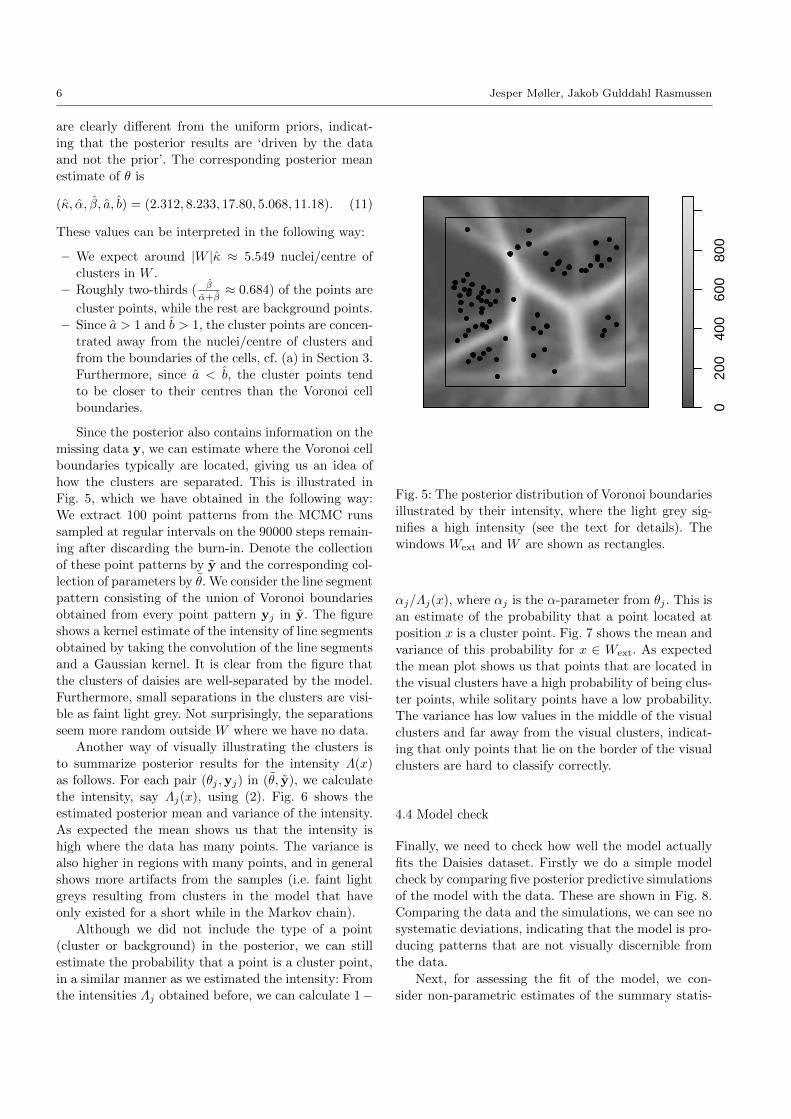
6 Jesper Møller, Jakob Gulddahl Rasmussen

are clearly different from the uniform priors, indicat-

ing that the posterior results are ‘driven by the dataand not the prior’. The corresponding posterior mean

estimate of θ is

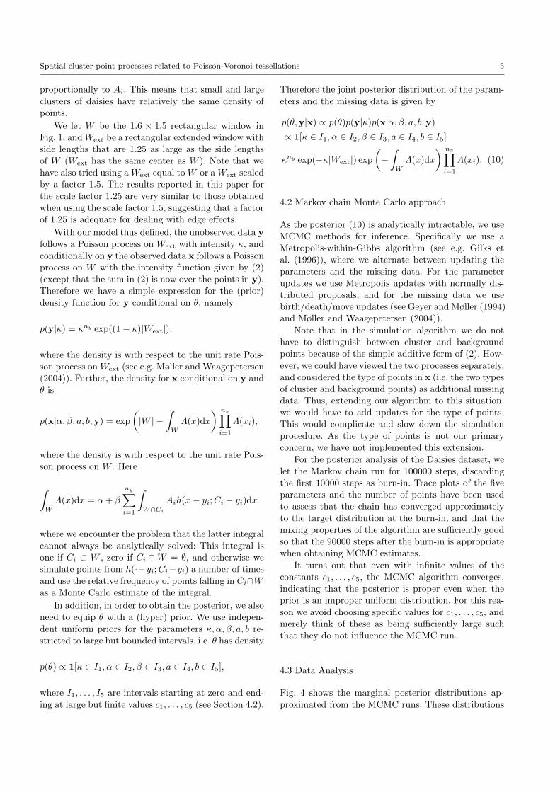
(κ, α, β, a, b) = (2.312, 8.233, 17.80, 5.068, 11.18). (11)

These values can be interpreted in the following way:

– We expect around |W |κ ≈ 5.549 nuclei/centre of

clusters in W .– Roughly two-thirds ( β

α+β≈ 0.684) of the points are

cluster points, while the rest are background points.– Since a > 1 and b > 1, the cluster points are concen-

trated away from the nuclei/centre of clusters and

from the boundaries of the cells, cf. (a) in Section 3.

Furthermore, since a < b, the cluster points tendto be closer to their centres than the Voronoi cell

boundaries.

Since the posterior also contains information on themissing data y, we can estimate where the Voronoi cell

boundaries typically are located, giving us an idea of

how the clusters are separated. This is illustrated inFig. 5, which we have obtained in the following way:

We extract 100 point patterns from the MCMC runs

sampled at regular intervals on the 90000 steps remain-

ing after discarding the burn-in. Denote the collectionof these point patterns by y and the corresponding col-

lection of parameters by θ. We consider the line segment

pattern consisting of the union of Voronoi boundariesobtained from every point pattern yj in y. The figure

shows a kernel estimate of the intensity of line segments

obtained by taking the convolution of the line segmentsand a Gaussian kernel. It is clear from the figure that

the clusters of daisies are well-separated by the model.

Furthermore, small separations in the clusters are visi-

ble as faint light grey. Not surprisingly, the separationsseem more random outside W where we have no data.

Another way of visually illustrating the clusters isto summarize posterior results for the intensity Λ(x)

as follows. For each pair (θj ,yj) in (θ, y), we calculate

the intensity, say Λj(x), using (2). Fig. 6 shows theestimated posterior mean and variance of the intensity.

As expected the mean shows us that the intensity is

high where the data has many points. The variance isalso higher in regions with many points, and in general

shows more artifacts from the samples (i.e. faint light

greys resulting from clusters in the model that have

only existed for a short while in the Markov chain).

Although we did not include the type of a point

(cluster or background) in the posterior, we can stillestimate the probability that a point is a cluster point,

in a similar manner as we estimated the intensity: From

the intensities Λj obtained before, we can calculate 1−

020

040

060

080

0

Fig. 5: The posterior distribution of Voronoi boundariesillustrated by their intensity, where the light grey sig-

nifies a high intensity (see the text for details). The

windows Wext and W are shown as rectangles.

αj/Λj(x), where αj is the α-parameter from θj . This is

an estimate of the probability that a point located atposition x is a cluster point. Fig. 7 shows the mean and

variance of this probability for x ∈ Wext. As expected

the mean plot shows us that points that are located inthe visual clusters have a high probability of being clus-

ter points, while solitary points have a low probability.

The variance has low values in the middle of the visual

clusters and far away from the visual clusters, indicat-ing that only points that lie on the border of the visual

clusters are hard to classify correctly.

4.4 Model check

Finally, we need to check how well the model actuallyfits the Daisies dataset. Firstly we do a simple model

check by comparing five posterior predictive simulations

of the model with the data. These are shown in Fig. 8.Comparing the data and the simulations, we can see no

systematic deviations, indicating that the model is pro-

ducing patterns that are not visually discernible from

the data.

Next, for assessing the fit of the model, we con-

sider non-parametric estimates of the summary statis-

Spatial cluster point processes related to Poisson-Voronoi tessellations 7

0 2 4 6 8

0.0

0.1

0.2

0.3

0.4

0 5 10 15 20

0.00

0.04

0.08

0.12

5 10 15 20 25 30 35

0.00

0.04

0.08

2 4 6 8 10 12

0.00

0.10

0.20

5 10 15 20 25 30

0.00

0.04

0.08

Fig. 4: Marginal posterior distributions of the parameters κ, α, β, a and b approximated by MCMC.

0.0 0.1 0.2 0.3

0.00

0.10

0.20

0.00 0.05 0.10 0.15 0.20

0.0

0.4

0.8

0.00 0.04 0.08 0.12

0.0

0.4

0.8

0.00 0.05 0.10 0.15 0.20

0.0

0.4

0.8

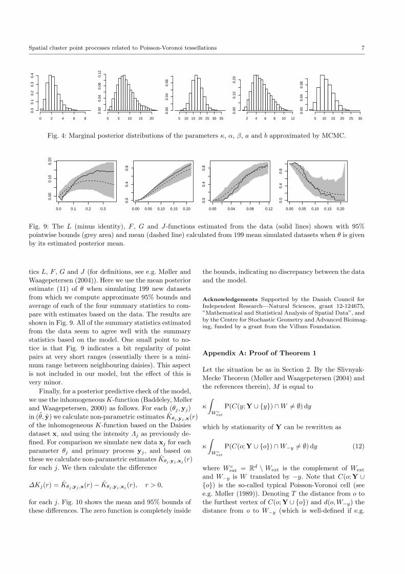
Fig. 9: The L (minus identity), F , G and J-functions estimated from the data (solid lines) shown with 95%

pointwise bounds (grey area) and mean (dashed line) calculated from 199 mean simulated datasets when θ is given

by its estimated posterior mean.

tics L, F , G and J (for definitions, see e.g. Møller and

Waagepetersen (2004)). Here we use the mean posterior

estimate (11) of θ when simulating 199 new datasets

from which we compute approximate 95% bounds andaverage of each of the four summary statistics to com-

pare with estimates based on the data. The results are

shown in Fig. 9. All of the summary statistics estimatedfrom the data seem to agree well with the summary

statistics based on the model. One small point to no-

tice is that Fig. 9 indicates a bit regularity of pointpairs at very short ranges (essentially there is a mini-

mum range between neighbouring daisies). This aspect

is not included in our model, but the effect of this is

very minor.

Finally, for a posterior predictive check of the model,we use the inhomogeneousK-function (Baddeley, Møller

and Waagepetersen, 2000) as follows. For each (θj ,yj)

in (θ, y) we calculate non-parametric estimates Kθj ,yj ,x(r)of the inhomogeneous K-function based on the Daisies

dataset x, and using the intensity Λj as previously de-

fined. For comparison we simulate new data xj for eachparameter θj and primary process yj , and based on

these we calculate non-parametric estimates Kθj ,yj ,xj(r)

for each j. We then calculate the difference

∆Kj(r) = Kθj ,yj ,x(r)− Kθj ,yj ,xj(r), r > 0,

for each j. Fig. 10 shows the mean and 95% bounds of

these differences. The zero function is completely inside

the bounds, indicating no discrepancy between the data

and the model.

Acknowledgements Supported by the Danish Council forIndependent Research—Natural Sciences, grant 12-124675,”Mathematical and Statistical Analysis of Spatial Data”, andby the Centre for Stochastic Geometry and Advanced Bioimag-ing, funded by a grant from the Villum Foundation.

Appendix A: Proof of Theorem 1

Let the situation be as in Section 2. By the Slivnyak-

Mecke Theorem (Møller and Waagepetersen (2004) and

the references therein), M is equal to

κ

∫

W cext

P(C(y;Y ∪ {y}) ∩W 6= ∅) dy

which by stationarity of Y can be rewritten as

κ

∫

W cext

P(C(o;Y ∪ {o}) ∩W−y 6= ∅) dy (12)

where W cext = Rd \ Wext is the complement of Wext

and W−y is W translated by −y. Note that C(o;Y ∪{o}) is the so-called typical Poisson-Voronoi cell (seee.g. Møller (1989)). Denoting T the distance from o to

the furthest vertex of C(o;Y ∪ {o}) and d(o,W−y) the

distance from o to W−y (which is well-defined if e.g.

8 Jesper Møller, Jakob Gulddahl Rasmussen

2040

6080

100

120

500

1500

2500

Fig. 6: Upper plot: Posterior mean of Λ(x). Lower plot:

Posterior variance of Λ(x). The windows Wext and W

are shown as rectangles in both plots.

0.2

0.4

0.6

0.8

0.05

0.1

0.15

Fig. 7: Posterior mean (upper) and variance (lower) of

the function 1 − α/Λ. The windows Wext and W are

shown as rectangles.

Spatial cluster point processes related to Poisson-Voronoi tessellations 9

Fig. 8: The upper left point pattern is the Daisies data,

while the other five point patterns are posterior predic-

tive simulations.

W−y is compact),

κ

∫

W cext

P(T > d(o,W−y)) dy (13)

is an upper bound for (12) and hence also for p.

In order to bound (13), we start by deriving a lowerbound on the cumulative distribution function (cdf)

of T . Denote σd = 2πd/2/Γ (d/2) the surface area of

the unit ball in Rd, and Fd the cdf of the Gamma-

distribution with shape parameter d and scale parame-ter 1.

Lemma 1 If W is compact, then

P(T > t) ≤ cd[1− Fd(κωdt

d)], t ≥ 0. (14)

Proof of Lemma 1:We shall ignore nullsets. With prob-

0.0 0.1 0.2 0.3

−0.

2−

0.1

0.0

0.1

0.2

0.3

Fig. 10: The difference of inhomogeneous K-functionscalculated from data and simulations shown by their

mean (solid line) and 95% bounds (grey area). The zero

function is indicated by a dashed line.

ability one, for all pairwise distinct points y1, . . . , yd ∈Y, the d-dimensional closed ball B(o, y1, . . . , yd) con-

taining o, y1, . . . , yd in its boundary is well-defined. De-note R(o, y1, . . . , yd) the radius ofB(o, y1, . . . , yd). Then

P(T > t) is at most

1

d!E

6=∑

y1,...,yd∈Y

1[B(o, y1, . . . , yd) ∩Y \ {y1, . . . , yd} = ∅,

R(o, y1, . . . , yd) > t]

where 6= over the summation sign means that y1, . . . , ydare pairwise distinct, and noting that the sum is almostsurely d! times the number of vertices in C(o;Y ∪ {o})with distance at least t to o. Therefore, by repeated use

of the Slivnyak-Mecke theorem, P(T > t) is at most

κd

d!

∫· · ·

∫P(B(o, y1, . . . , yd) ∩Y = ∅,

R(o, y1, . . . , yd) > t) dy1 · · · dydand hence, since Y is a stationary Poisson process andB(o, y1, . . . , yd) has volume ωdR(o, y1, . . . , yd)

d, P(T >

t) is at most

κd

d!

∫· · ·

∫1[R(o, y1, . . . , yd) > t]

exp(−κωdR(o, y1, . . . , yd)

d)dy1 · · · dyd

=κd

d!

1

|A|

∫ ∫· · ·

∫1[y0 ∈ A, R(y0, y1, . . . , yd) > t]

exp(−κωdR(y0, y1, . . . , yd)

d)dy0dy1 · · · dyd

10 Jesper Møller, Jakob Gulddahl Rasmussen

where A ⊂ Rd is an arbitrary Borel with volume 0 <

|A| < ∞, and where R = R(y0, y1, . . . , yd) is the ra-dius of the d-dimensional closed ball B(y0, y1, . . . , yd)

containing y0, y1, . . . , yd in its boundary (which is well-

defined for Lebesgue almost all (y0, y1, . . . , yd) ∈ Rd(d+1)).Denote z = z(y0, y1, . . . , yd) the centre ofB(y0, y1, . . . , yd),

ui = ui(y0, y1, . . . , yd) the unit vector such that yi =

z+Rui (i = 0, 1, . . . , d), ∆(u0, u1, . . . , ud) the volume ofthe convex hull of u0, u1, . . . , ud, and ν surface measure

on the unit sphere in Rd. Then, by Blasche-Petkantschin’s

formula (e.g. Miles (1971)), P(T > t) is at most

κd

|A|

∫ ∫ ∫ ∫· · ·

∫1[z +Ru0 ∈ A, R > t]Rd2−1

exp(−κωdR

d)∆(u0, u1, . . . , ud)

dz dRν(du0) ν(du1) · · · ν(dud)

which reduces to

κd

∫ ∞

t

Rd2−1 exp(−κωdR

d)dR

∫ ∫· · ·

∫∆(u0, u1, . . . , ud) ν(du0) ν(du1) · · · ν(dud).

Thereby, since

∫ ∞

t

Rd2−1 exp(−κωdR

d)dR

=(d− 1)!

d(κωd)d[1− F (d(κωdt

d))]

and

∫ ∫· · ·

∫∆(u0, u1, . . . , ud) ν(du0) ν(du1) · · · ν(dud)

=2d+1π(d2+d−1)/2Γ ((d2 + 1)/2)

d!Γ (d2/2)Γ ((d+ 1)/2)d

(see Theorem 2 in Miles (1971)), we obtain (14) after a

straightforward calculation.

Proof of Theorem 1: It suffices to consider the case

where W = b(z, r1). Then p is at most

κ

∫

‖z−y‖≥r2

P(T > d(o, b(z − y, r1))) dy

≤ κcd

∫

‖y‖>r2

∫ ∞

κωd(‖y‖−r1)dfd(t) dt dy

where the inequality follows from Lemma 1. Hence, us-ing Fubini’s theorem, a shift for y to hyperspherical co-

ordinates in Rd, and the fact that ωd = σd/d, we easily

deduce the result.

Appendix B: Moment results

Since X is a Cox process driven by (2), moment re-sults for X are inherited from the distribution of the

primary point process Y. In particular, X has inten-

sity ρ = EΛ(o) and pair correlation function g(x) =E [Λ(o)Λ(x)] /ρ2, x ∈ Rd (provided these expectations

exist), see e.g. Møller and Waagepetersen (2004). This

appendix discusses the expressions of ρ and g.

Recall the notion of the typical Voronoi cell: Let Π

denote the space of compact convex polytopes C ⊂ Rd

with |C| > 0 and o ∈ intC (we equip Π with the usual

σ-algebra for closed subsets of Rd restricted to Π, i.e.

the σ-algebra generated by the sets {C ∈ Π : C ∩K =

∅} for all compact K ⊂ Rd). The typical Voronoi cell isa random variable C with state spaceΠ and distribution

P (C ∈ F ) = E∑

i

1[yi ∈ B, Ci − yi ∈ F ]/(κ|B|) (15)

where B ⊂ Rd is an arbitrary (Borel) set with 0 < |B| <∞ (by stationarity of Y, the right hand side in (15)does not depend on the choice of B). Intuitively, C is a

randomly chosen cell viewed from its nucleus; formally,

(15) is the Palm distribution of a Voronoi cell. It followsby standard measure theoretical considerations that

E∑

i

f(yi, Ci − yi) = κE

∫f(y, C) dy (16)

for any nonnegative (measurable) function f , and let-

ting A = |C|, then EA = 1/κ. See e.g. Møller (1989).

Since Y is a stationary Poisson process, by the Sliv-

nyak-Mecke formula (see e.g. Møller andWaagepetersen

(2004)),

E∑

i

f(yi,Y) = κE

∫f(y,Y ∪ {y}) dy (17)

for any nonnegative (and measurable) function f . By

(16)-(17) and stationarity of Y, we can then take

C = C(o;Y ∪ {o}). (18)

Proposition 1 If Ek(A) < ∞, then

ρ = α+ βκEk(A) (19)

is finite.

Proof: By (2),

EΛext(o) = α+βE∑

i

1[−yi ∈ Ci−yi]k(Ai)h(−yi, Ci−yi).

Spatial cluster point processes related to Poisson-Voronoi tessellations 11

Combining this with (16) and the facts that ρ = EΛext(o)

and |Ci| = |Ci − yi|, we obtain that ρ is equal to

= α+ βE∑

i

1[−yi ∈ Ci − yi]k(|Ci − yi|)h(−yi, Ci − yi)

= α+ βκE

∫1[−y ∈ C]k(A)h(−yi, C) dy

= α+ βκEk(A)

whereby the assertion follows.

The pair correlation function g is more complicatedto evaluate. For example, let k be the identity function.

Then by similar arguments as in the proof of Proposi-

tion 1 and by using (17) and (18), we obtain

E [Λ(o)Λ(x)]

=α2 + 2αρ+ β2κE

∫1[{y, x+ y} ⊂ C]|C|2h(y, C)

h(x+ y, C) dy + (βκ)2E

∫ ∫

1[o ∈ C(y1;Y ∪ {y1, y2}), x ∈ C(y2;Y ∪ {y1, y2})]|C(y1;Y ∪ {y1, y2})||C(y2;Y ∪ {y1, y2})|h(−y1;C(y1;Y ∪ {y1, y2})− y1)

h(x− y2;C(y2;Y ∪ {y1, y2})− y2) dy1 dy2.

Here the first mean value corresponds to the case where

two secondary points with locations o and x belong tothe same cell, and the second mean value corresponds

to the case where they belong to two different cells. We

are not aware of any analytic methods for evaluatingthese mean values, even if h(·;C) is uniform on C, in

which case

E [Λ(o)Λ(x)]

=α2 + 2αρ+ β2κ

∫P ({y, x+ y} ⊂ C(o;Φ ∪ {o})) dy+

(βκ)2∫ ∫

P (o ∈ C(y1;Y ∪ {y1, y2}),

x ∈ C(y2;Y ∪ {y1, y2})) dy1 dy2

=α2 + 2αρ+ β2κ

∫exp (−κ|b(o,max{‖y‖, ‖x+ y‖})|)

dy + (βκ)2∫ ∫

1[‖y1‖ ≤ ‖y2‖, ‖y2 − x‖ ≤ ‖y1 − x‖]

exp (−κ|b(o, ‖y1‖) ∪ b(x, ‖y2 − x‖)|) dy1 dy2where the integrals may be evaluated by numerical meth-ods.

References

1. Baddeley B, Møller J, Waagepetersen R (2000) Non-and semi-parametric estimation of interaction in inhomo-geneous point patterns. Statistica Neerlandica 54: 329–350

2. Baddeley A, Turner R (2005). Spatstat: an R package foranalyzing spatial point patterns. J. Statist. Software 12: 1–42

3. Barr C, Schoenberg FP (2010) On the Voronoi estimatorfor the intensity of an inhomogeneous planar Poisson pro-cess. Biometrika 97: 977–984

4. Blackwell PG (2001) Bayesian inference for a random tes-sellation process. Biometrics 57: 502–507

5. Blackwell PG, Møller J (2003) Bayesian analysis of de-formed tessellation models. Adv. Appl. Probab. 35: 4–26

6. Byers SD, Raftery AE (2002) Bayesian estimation and seg-mentation of spatial point processes using Voronoi tilings.In: Lawson AG, Denison DGT (eds) Spatial cluster mod-elling, Chapman & Hall/CRC Press, London

7. Cox DR (1955) Some statistical models related with seriesof events. J. Roy. Statist. Soc. B 17: 129–164

8. Foss SG, Zuyev SA (1996) On a Voronoi Aggregative Pro-cess Related to a Bivariate Poisson Process. Adv. Appl.Probab. 28: 965–981

9. Geyer CJ, Møller J (1994) Simulation procedures andlikelihood inference for spatial point processes. Scand. J.Statist. 21: 359–373

10. Gilks WR, Richardson S, and Spiegelhalter DJ (1996)Markov Chain Monte Carlo in Practice. Chapman & Hall,London

11. Heikkinen J, Arjas E (1998) Non-parametric Bayesianestimation of a spatial Poisson intensity. Scand. J. Statist.25: 435–450

12. Miles RE (1971) Isotropic random simplices. Adv. Appl.Probab. 3: 353–382.

13. Møller J (1989) Random tessellations in Rd. Adv. Appl.Probab. 21: 37–73

14. Møller J, Rasmussen JG (2012) A sequential point pro-cess model and Bayesian inference for spatial point patternswith linear structures. Scand. J. Statist. 39: 618–634

15. Møller J, Waagepetersen RP (2004) Statistical inferenceand simulation for spatial point processes. Chapman andHall/CRC, Boca Raton

16. Møller J, Waagepetersen RP (2007) Modern spatial pointprocess modelling and inference (with discussion). Scand. J.Statist. 34: 643-711

17. Okabe A, Boots B, Sugihara K, Chiu SN (2000) Spa-tial tessellations. Concepts and applications of Voronoi di-agrams, 2nd. Wiley, Chichester

18. Skare Ø, Møller J, Jensen EBV (2007) Bayesian analysisof spatial point processes in the neighbourhood of Voronoinetworks. Statist. Comp. 17: 369–379