Fluid flow modelling with seismic cluster analysis - … · Fluid flow modelling with seismic...
12
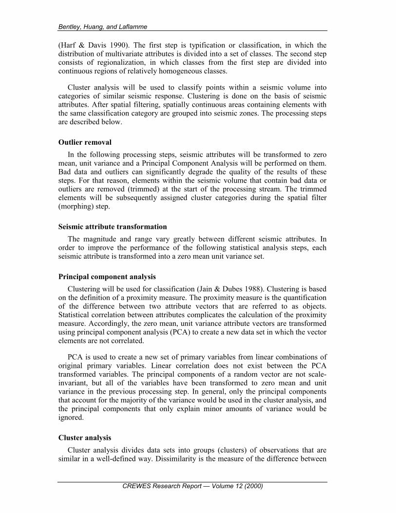
Fluid flow modelling with seismic cluster analysis CREWES Research Report Volume 12 (2000) Fluid flow modelling with seismic cluster analysis Laurence R. Bentley, Xuri Huang 1 and Claude Laflamme 2 ABSTRACT Cluster analysis is used to construct fluid flow zones from seismic attributes. The steps are: 1. Remove grid points that contain outliers in any seismic attribute; 2. Scale each attribute to zero mean and unit variance; 3. Use principal component analysis to transform the scaled attributes to uncorrelated principal component attributes; 4. Principal component attributes are grouped into categories of similar seismic response using cluster analysis; 5. Upscale the seismic grid to the computational grid scale using a weighted voting procedure (morphing); 6. Spatially filter cluster assignments to remove small, isolated spots using a weighted voting scheme; 7. Assign a seismic zone to spatially connected elements with the same cluster category. Using a Gulf of Mexico test case, the zoning procedure produced useful computational zones and reduced the time required for history matching. INTRODUCTION Subsurface flow simulation models require the specification of permeability and porosity at every node within the computational mesh. The values of permeability and porosity are not known with high precision because data are only sparsely sampled, interpolations are inexact, the scale of permeability measurements is different from the scale of the computational mesh and measurements are inexact. Consequently flow simulators must be calibrated. Optimization techniques can be used to perform calibrations. The number of elements in a computational mesh can be in the tens of thousands so that the optimization problem is computationally intractable. One approach for alleviating the problem of high dimensionality is to group nodes into spatially continuous zones that are updated as a group. In general this has been done on an ad hoc basis. In the following, a methodology is described for using a spatially dense set of geophysical attributes to create spatial zones. The fundamental assumption is that spatially continuous areas of similar geophysical response are areas of relatively homogeneous hydraulic properties. The method will be applied to a 3D seismic data set acquired over a field in the Gulf of Mexico. THEORETICAL OVERVIEW It is assumed that a geologic interpretation has defined the geometry of the aquifer boundaries and significant, well-defined lithologic units. A geologic mapping is then conducted within these boundaries. The process of geologic mapping, or, in the present case zone definition, involves the identification of homogeneous regions 1 Western Geophysical Company 2 Department of Mathematics, University of Calgary
Transcript of Fluid flow modelling with seismic cluster analysis - … · Fluid flow modelling with seismic...

Fluid flow modelling with seismic cluster analysis
CREWES Research Report � Volume 12 (2000)
Fluid flow modelling with seismic cluster analysis
Laurence R. Bentley, Xuri Huang1 and Claude Laflamme2
ABSTRACT Cluster analysis is used to construct fluid flow zones from seismic attributes. The steps are: 1. Remove grid points that contain outliers in any seismic attribute; 2. Scale each attribute to zero mean and unit variance; 3. Use principal component analysis to transform the scaled attributes to uncorrelated principal component attributes; 4. Principal component attributes are grouped into categories of similar seismic response using cluster analysis; 5. Upscale the seismic grid to the computational grid scale using a weighted voting procedure (morphing); 6. Spatially filter cluster assignments to remove small, isolated spots using a weighted voting scheme; 7. Assign a seismic zone to spatially connected elements with the same cluster category. Using a Gulf of Mexico test case, the zoning procedure produced useful computational zones and reduced the time required for history matching.
INTRODUCTION Subsurface flow simulation models require the specification of permeability and
porosity at every node within the computational mesh. The values of permeability and porosity are not known with high precision because data are only sparsely sampled, interpolations are inexact, the scale of permeability measurements is different from the scale of the computational mesh and measurements are inexact. Consequently flow simulators must be calibrated. Optimization techniques can be used to perform calibrations.
The number of elements in a computational mesh can be in the tens of thousands so that the optimization problem is computationally intractable. One approach for alleviating the problem of high dimensionality is to group nodes into spatially continuous zones that are updated as a group. In general this has been done on an ad hoc basis.
In the following, a methodology is described for using a spatially dense set of geophysical attributes to create spatial zones. The fundamental assumption is that spatially continuous areas of similar geophysical response are areas of relatively homogeneous hydraulic properties. The method will be applied to a 3D seismic data set acquired over a field in the Gulf of Mexico.
THEORETICAL OVERVIEW It is assumed that a geologic interpretation has defined the geometry of the aquifer
boundaries and significant, well-defined lithologic units. A geologic mapping is then conducted within these boundaries. The process of geologic mapping, or, in the present case zone definition, involves the identification of homogeneous regions 1 Western Geophysical Company 2 Department of Mathematics, University of Calgary
Bentley, Huang, and Laflamme
CREWES Research Report � Volume 12 (2000)
(Harf & Davis 1990). The first step is typification or classification, in which the distribution of multivariate attributes is divided into a set of classes. The second step consists of regionalization, in which classes from the first step are divided into continuous regions of relatively homogeneous classes.
Cluster analysis will be used to classify points within a seismic volume into categories of similar seismic response. Clustering is done on the basis of seismic attributes. After spatial filtering, spatially continuous areas containing elements with the same classification category are grouped into seismic zones. The processing steps are described below.
Outlier removal In the following processing steps, seismic attributes will be transformed to zero
mean, unit variance and a Principal Component Analysis will be performed on them. Bad data and outliers can significantly degrade the quality of the results of these steps. For that reason, elements within the seismic volume that contain bad data or outliers are removed (trimmed) at the start of the processing stream. The trimmed elements will be subsequently assigned cluster categories during the spatial filter (morphing) step.
Seismic attribute transformation The magnitude and range vary greatly between different seismic attributes. In
order to improve the performance of the following statistical analysis steps, each seismic attribute is transformed into a zero mean unit variance set.
Principal component analysis Clustering will be used for classification (Jain & Dubes 1988). Clustering is based
on the definition of a proximity measure. The proximity measure is the quantification of the difference between two attribute vectors that are referred to as objects. Statistical correlation between attributes complicates the calculation of the proximity measure. Accordingly, the zero mean, unit variance attribute vectors are transformed using principal component analysis (PCA) to create a new data set in which the vector elements are not correlated.
PCA is used to create a new set of primary variables from linear combinations of original primary variables. Linear correlation does not exist between the PCA transformed variables. The principal components of a random vector are not scale-invariant, but all of the variables have been transformed to zero mean and unit variance in the previous processing step. In general, only the principal components that account for the majority of the variance would be used in the cluster analysis, and the principal components that only explain minor amounts of variance would be ignored.
Cluster analysis Cluster analysis divides data sets into groups (clusters) of observations that are
similar in a well-defined way. Dissimilarity is the measure of the difference between
Fluid flow modelling with seismic cluster analysis
CREWES Research Report � Volume 12 (2000)
two data points. The partitioning algorithm CLARA (Chapter 3 Kaufman & Rousseeuw 1990) is used to perform the clustering. CLARA creates a partitioning clustering as opposed to a hierarchical clustering. The advantage of the algorithm is that it requires significantly less storage and memory than hierarchical algorithms, so that CLARA can deal with very large datasets.
The results presented in this paper are based on the dissimilarity measure:
( )∑
=−=
PN
1j
2Pjk
Pjllk aad
(1)
where dlk is the dissimilarity between the lth and kth objects (transformed attribute vectors associated with a location in the seismic data volume), PN is the number of retained principal components and P
jla is the jth principal component element of the lth object. Other dissimilarity measures are possible and more work remains to define the optimal clustering norm. Superscript P is to indicate principal component data as opposed to the original data.
Spatial Filter (morphing) Spatial filtering is used to remove small, isolated areas of a single cluster category
and to upscale the cluster categories of the geophysical data grid to the computational grid.
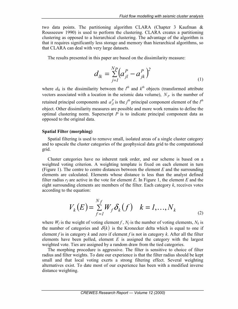
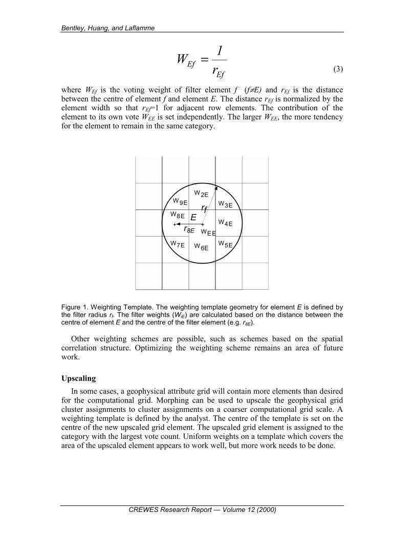
Cluster categories have no inherent rank order, and our scheme is based on a weighted voting criterion. A weighting template is fixed on each element in turn (Figure 1). The centre to centre distances between the element E and the surrounding elements are calculated. Elements whose distance is less than the analyst defined filter radius rf are active in the vote for element E. In Figure 1, the element E and the eight surrounding elements are members of the filter. Each category k, receives votes according to the equation:
( ) ( ) k
fN
1fkfk N1kfWEV ,,…== ∑
=δ
(2)
where Wf is the weight of voting element f , Nf is the number of voting elements, Nk is the number of categories and ( )kδ is the Kronecker delta which is equal to one if element f is in category k and zero if element f is not in category k. After all the filter elements have been polled, element E is assigned the category with the largest weighted vote. Ties are assigned by a random draw from the tied categories.
The morphing procedure is aggressive. The filter is sensitive to choice of filter radius and filter weights. To date our experience is that the filter radius should be kept small and that local voting exerts a strong filtering effect. Several weighting alternatives exist. To date most of our experience has been with a modified inverse distance weighting.
Bentley, Huang, and Laflamme
CREWES Research Report � Volume 12 (2000)
Ef
Ef r1W =
(3)
where WEf is the voting weight of filter element f (f≠E) and rEf is the distance between the centre of element f and element E. The distance rEf is normalized by the element width so that rEf=1 for adjacent row elements. The contribution of the element to its own vote WEE is set independently. The larger WEE, the more tendency for the element to remain in the same category.
Erf
WEE
W 2EW3E
W4E
W5EW 6EW7E
W8E
W9E
++ r8E
Figure 1. Weighting Template. The weighting template geometry for element E is defined by the filter radius rf. The filter weights (WiE) are calculated based on the distance between the centre of element E and the centre of the filter element (e.g. r8E).
Other weighting schemes are possible, such as schemes based on the spatial correlation structure. Optimizing the weighting scheme remains an area of future work.
Upscaling In some cases, a geophysical attribute grid will contain more elements than desired
for the computational grid. Morphing can be used to upscale the geophysical grid cluster assignments to cluster assignments on a coarser computational grid scale. A weighting template is defined by the analyst. The centre of the template is set on the centre of the new upscaled grid element. The upscaled grid element is assigned to the category with the largest vote count. Uniform weights on a template which covers the area of the upscaled element appears to work well, but more work needs to be done.
Fluid flow modelling with seismic cluster analysis
CREWES Research Report � Volume 12 (2000)
Removing small features (spot removal) Small, isolated groups of elements with the same cluster category will yield zones
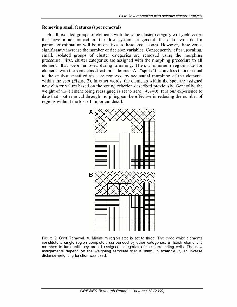
that have minor impact on the flow system. In general, the data available for parameter estimation will be insensitive to these small zones. However, these zones significantly increase the number of decision variables. Consequently, after upscaling, small, isolated groups of cluster categories are removed using the morphing procedure. First, cluster categories are assigned with the morphing procedure to all elements that were removed during trimming. Then, a minimum region size for elements with the same classification is defined. All �spots� that are less than or equal to the analyst specified size are removed by sequential morphing of the elements within the spot (Figure 2). In other words, the elements within the spot are assigned new cluster values based on the voting criterion described previously. Generally, the weight of the element being reassigned is set to zero (WEE=0). It is our experience to date that spot removal through morphing can be effective in reducing the number of regions without the loss of important detail.
Figure 2. Spot Removal. A. Minimum region size is set to three. The three white elements constitute a single region completely surrounded by other categories. B. Each element is morphed in turn until they are all assigned categories of the surrounding cells. The new assignments depend on the weighting template that is used. In example B, an inverse distance weighting function was used.

Bentley, Huang, and Laflamme
CREWES Research Report � Volume 12 (2000)
Regionalization Regionalization is the process of forming geometrically continuous zones of
relatively homogeneous classification. This process requires the definition of boundaries between zones of homogeneous classification. The boundaries will then define the geometric limit of zones. The zones must be indexed and every element in the computational mesh is assigned to an indexed zone. Regionalization is performed using a simple search algorithm. The search begins at an element which has not been assigned a zone and continues until another connected element of the same cluster category cannot be found. A node can be connected along an element face, edge or corner. For example, the three white elements in Figure 2A would be classified as a zone with three elements.
EXAMPLE Data from a three-dimensional seismic survey in the Gulf of Mexico will be used
to demonstrate the method. The survey was conducted over a turbidite sheet sand reservoir offshore Louisiana before production (Huang et al. 1997). The data from the top of the target zone was extracted and used to perform a 2-D seismic zonation for eventual use in a flow model. There are 15,306 seismic elements in the areal two-dimensional grid that covers the survey area.
From the many possible seismic attributes, seven were chosen for use in the seismic zonation procedure. Clusters were created using instantaneous phase, instantaneous amplitude, instantaneous frequency, amplitude weighted frequency, energy weighted instantaneous frequency, average energy and arithmetic mean. These attributes were chosen because previous work indicated that they were the most sensitive to changes in porosity.
Clustering Data was trimmed and each attribute was transformed into a zero mean unit
variance equivalent. PCA analysis was performed on the trimmed, transformed data, and the objects were clustered into seven categories based on the dissimilarity measure of equation (1) using all seven principal components. The trimmed elements were reassigned by morphing with a template radius of 1.5 blocks (i.e. 9 element template shown in Figure 1) and all voting weights equal to one. A voting radius of 1.5 is used because it is greater than the square root of two, so corner elements are included, but less than 2 so the next layer of elements is excluded. The results are shown in Figure 3. The 15,306 seismic elements are reduced to 2,504 regions after clustering and regionalization. The number of decision regions has been reduced by a factor of six, but it is still large.
Morphing Many small regions exist that are not hydraulically signficant at the field scale.
Consequently, the clustered data will be spatially filtered to remove sequentially larger and larger isolated spots until significant structure is lost. In this way, the number of seismic zones will be reduced, without affecting the ability of the simulator to capture the aspects of flow required in the parameter estimation step. In
Fluid flow modelling with seismic cluster analysis
CREWES Research Report � Volume 12 (2000)
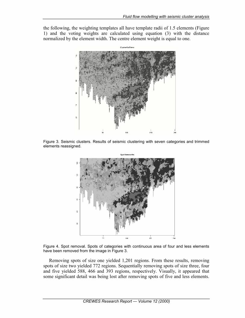
the following, the weighting templates all have template radii of 1.5 elements (Figure 1) and the voting weights are calculated using equation (3) with the distance normalized by the element width. The centre element weight is equal to one.
Figure 3. Seismic clusters. Results of seismic clustering with seven categories and trimmed elements reassigned.
Figure 4. Spot removal. Spots of categories with continuous area of four and less elements have been removed from the image in Figure 3.
Removing spots of size one yielded 1,201 regions. From these results, removing spots of size two yielded 772 regions. Sequentially removing spots of size three, four and five yielded 588, 466 and 393 regions, respectively. Visually, it appeared that some significant detail was being lost after removing spots of five and less elements.
Bentley, Huang, and Laflamme
CREWES Research Report � Volume 12 (2000)
The results after removing regions of four and less elements were deemed appropriate for flow modelling and they are shown in Figure 4.
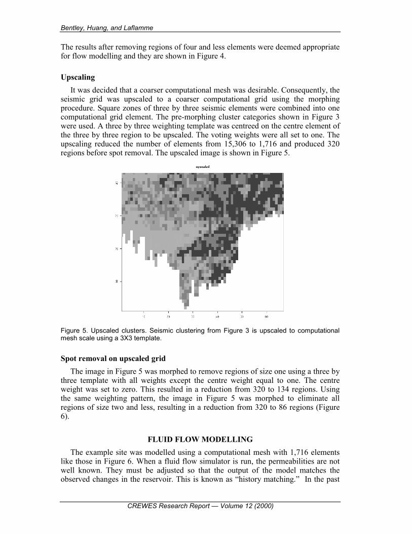
Upscaling It was decided that a coarser computational mesh was desirable. Consequently, the
seismic grid was upscaled to a coarser computational grid using the morphing procedure. Square zones of three by three seismic elements were combined into one computational grid element. The pre-morphing cluster categories shown in Figure 3 were used. A three by three weighting template was centreed on the centre element of the three by three region to be upscaled. The voting weights were all set to one. The upscaling reduced the number of elements from 15,306 to 1,716 and produced 320 regions before spot removal. The upscaled image is shown in Figure 5.
Figure 5. Upscaled clusters. Seismic clustering from Figure 3 is upscaled to computational mesh scale using a 3X3 template.
Spot removal on upscaled grid The image in Figure 5 was morphed to remove regions of size one using a three by
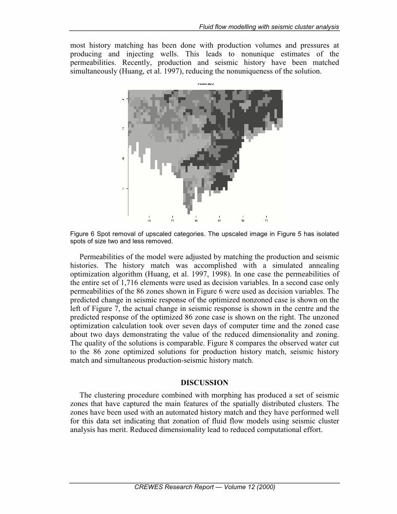
three template with all weights except the centre weight equal to one. The centre weight was set to zero. This resulted in a reduction from 320 to 134 regions. Using the same weighting pattern, the image in Figure 5 was morphed to eliminate all regions of size two and less, resulting in a reduction from 320 to 86 regions (Figure 6).
FLUID FLOW MODELLING The example site was modelled using a computational mesh with 1,716 elements
like those in Figure 6. When a fluid flow simulator is run, the permeabilities are not well known. They must be adjusted so that the output of the model matches the observed changes in the reservoir. This is known as �history matching.� In the past
Fluid flow modelling with seismic cluster analysis
CREWES Research Report � Volume 12 (2000)
most history matching has been done with production volumes and pressures at producing and injecting wells. This leads to nonunique estimates of the permeabilities. Recently, production and seismic history have been matched simultaneously (Huang, et al. 1997), reducing the nonuniqueness of the solution.
Figure 6 Spot removal of upscaled categories. The upscaled image in Figure 5 has isolated spots of size two and less removed.
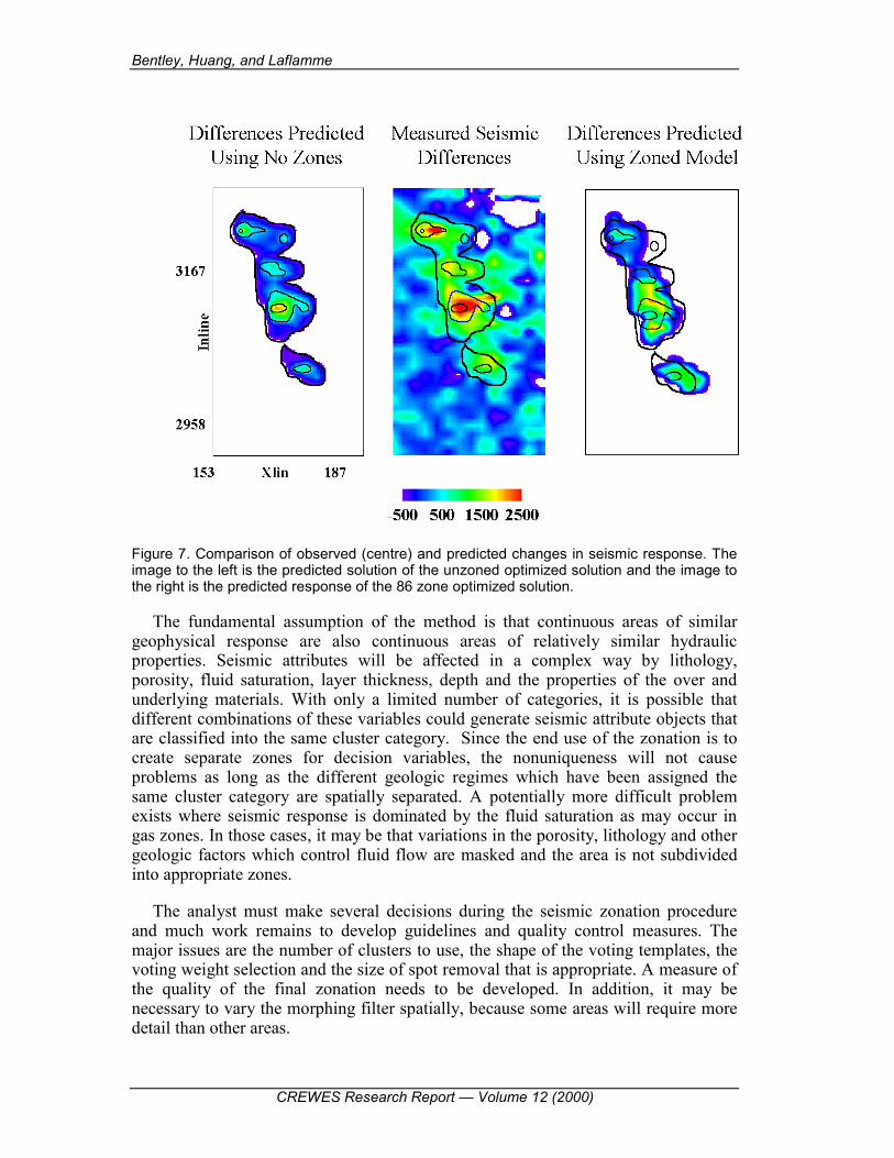
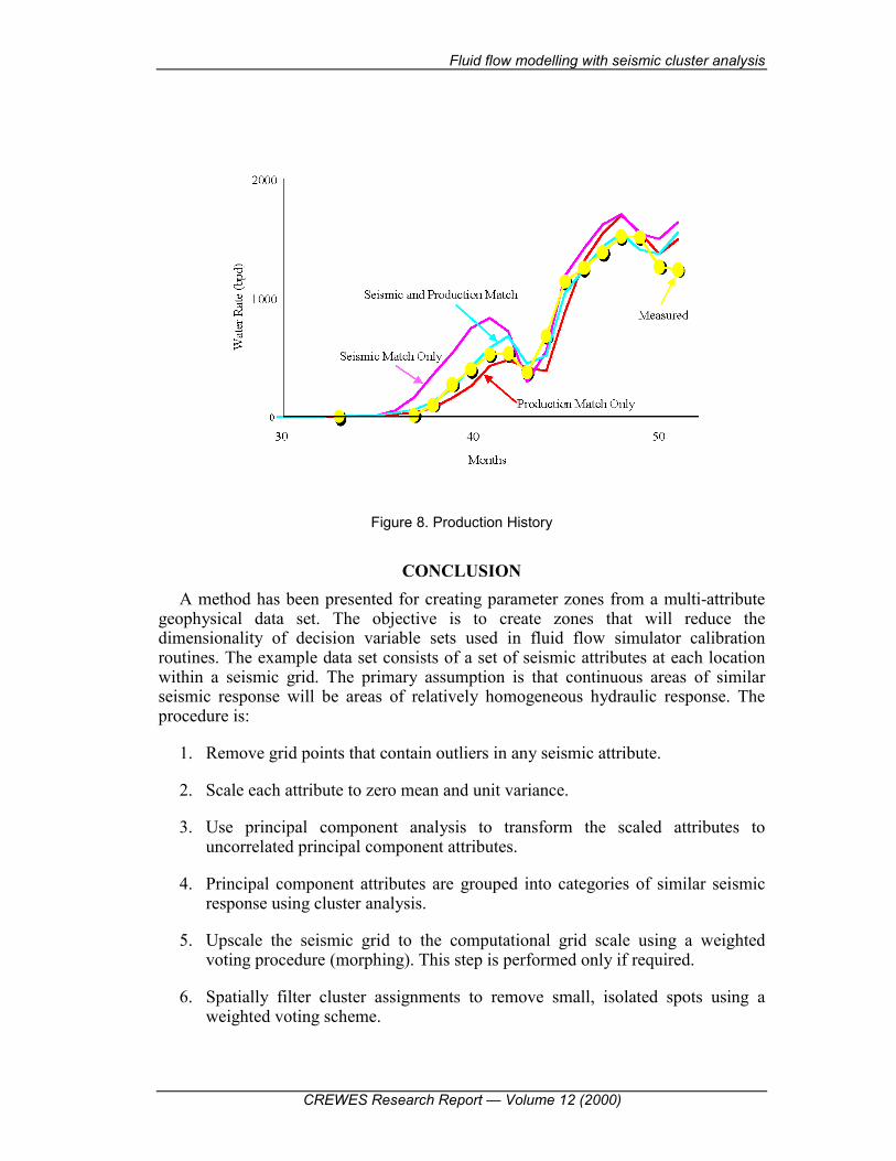
Permeabilities of the model were adjusted by matching the production and seismic histories. The history match was accomplished with a simulated annealing optimization algorithm (Huang, et al. 1997, 1998). In one case the permeabilities of the entire set of 1,716 elements were used as decision variables. In a second case only permeabilities of the 86 zones shown in Figure 6 were used as decision variables. The predicted change in seismic response of the optimized nonzoned case is shown on the left of Figure 7, the actual change in seismic response is shown in the centre and the predicted response of the optimized 86 zone case is shown on the right. The unzoned optimization calculation took over seven days of computer time and the zoned case about two days demonstrating the value of the reduced dimensionality and zoning. The quality of the solutions is comparable. Figure 8 compares the observed water cut to the 86 zone optimized solutions for production history match, seismic history match and simultaneous production-seismic history match.
DISCUSSION The clustering procedure combined with morphing has produced a set of seismic
zones that have captured the main features of the spatially distributed clusters. The zones have been used with an automated history match and they have performed well for this data set indicating that zonation of fluid flow models using seismic cluster analysis has merit. Reduced dimensionality lead to reduced computational effort.
Bentley, Huang, and Laflamme
CREWES Research Report � Volume 12 (2000)
Figure 7. Comparison of observed (centre) and predicted changes in seismic response. The image to the left is the predicted solution of the unzoned optimized solution and the image to the right is the predicted response of the 86 zone optimized solution.
The fundamental assumption of the method is that continuous areas of similar geophysical response are also continuous areas of relatively similar hydraulic properties. Seismic attributes will be affected in a complex way by lithology, porosity, fluid saturation, layer thickness, depth and the properties of the over and underlying materials. With only a limited number of categories, it is possible that different combinations of these variables could generate seismic attribute objects that are classified into the same cluster category. Since the end use of the zonation is to create separate zones for decision variables, the nonuniqueness will not cause problems as long as the different geologic regimes which have been assigned the same cluster category are spatially separated. A potentially more difficult problem exists where seismic response is dominated by the fluid saturation as may occur in gas zones. In those cases, it may be that variations in the porosity, lithology and other geologic factors which control fluid flow are masked and the area is not subdivided into appropriate zones.
The analyst must make several decisions during the seismic zonation procedure and much work remains to develop guidelines and quality control measures. The major issues are the number of clusters to use, the shape of the voting templates, the voting weight selection and the size of spot removal that is appropriate. A measure of the quality of the final zonation needs to be developed. In addition, it may be necessary to vary the morphing filter spatially, because some areas will require more detail than other areas.
Fluid flow modelling with seismic cluster analysis
CREWES Research Report � Volume 12 (2000)
Figure 8. Production History
CONCLUSION A method has been presented for creating parameter zones from a multi-attribute
geophysical data set. The objective is to create zones that will reduce the dimensionality of decision variable sets used in fluid flow simulator calibration routines. The example data set consists of a set of seismic attributes at each location within a seismic grid. The primary assumption is that continuous areas of similar seismic response will be areas of relatively homogeneous hydraulic response. The procedure is:
1. Remove grid points that contain outliers in any seismic attribute.
2. Scale each attribute to zero mean and unit variance.
3. Use principal component analysis to transform the scaled attributes to uncorrelated principal component attributes.
4. Principal component attributes are grouped into categories of similar seismic response using cluster analysis.
5. Upscale the seismic grid to the computational grid scale using a weighted voting procedure (morphing). This step is performed only if required.
6. Spatially filter cluster assignments to remove small, isolated spots using a weighted voting scheme.

Bentley, Huang, and Laflamme
CREWES Research Report � Volume 12 (2000)
7. Assign a seismic zone to spatially connected elements with the same cluster category.
The procedure was applied to a data set collected over a turbidite sand sheet located in the Gulf of Mexico. The 15,306 points in the seismic grid were reduced to 466 regions with the removal of regions of size 4 and less while maintaining the main structure of the original cluster category map. An upscaled cluster map for use with a computational grid was constructed from a three by three element upscaling using the morphing procedure. After removing regions of two and less elements, the 1,716 elements contained 86 seismic zones. Visually, these zones look suitable for use in a fluid flow simulator. The zoned computational grid provided production and seismic history matches that were similar in quality to the unzoned grid. The reduction in dimensionality significantly reduced the computational effort required to achieve the history matches.
ACKNOWLEDGEMENTS The authors wish to thank Natural Sciences and Engineering Research Council of
Canada (NSERC), the Pacific Institute for Mathematical Sciences (PIMS), Western Geophysical Company, and the CREWES sponsors for supporting this work. We also thank Shell Offshore Oil Inc. for providing the raw seismic data set.
REFERENCES Harf`, J. & Davis, J.C., 1990. Regionalization in geology by multivariate classification. Math. Geol.
22(5): 573-588. Huang, X., Meister, L., & Workman, R., 1997. Reservoir characterization by integration of time-lapse
seismic and production data, In proc. SPE Annual Technical Conf. San Antonio 5-8 Oct., 1997, SPE 38695.
Huang, X., Meister, L., & Workman, R., 1998. Improvement and sensitivity of reservoir characterization derived from time-lapse seismic data, In proc. SPE Annual Technical Conf. New Orleans 27-30 Sept., 1998, SPE 49146.
Jain, A.K. & Dubes, R.C., 1988. Algorithms for clustering data. Englewood Cliffs: Prentice-Hall. Kaufman, L. & Rousseeuw, P.J., 1990. Finding groups in data: an introduction to cluster analysis. New
York: Wiley.