CLIMATOLOGICAL APPLICATIONS

IN TURKEY

Serhat SENSOY, Mesut DEMİRCAN Engineer

Climatology Division

May 2010, ANKARA

REPUPLIC of TURKEY MINISTRY OF ENVIRONMENT and FORESTRY

TURKISH STATE METEOROLOGICAL SERVICE

CLIMATOLOGICAL APPLICATIONS IN TURKEY

Serhat SENSOY, Mesut DEMİRCAN Engineer

Climatology Division klimatoloji@dmi.gov.tr

May 2010, ANKARA

Contents Page

Introduction

1. Defination of climate and climatology………………………………... 1 1.1. Climate ………………………………………………………... …. 1 1.2. Climatology ………………………..………………………… …. 2

2. Climatological division …………………………………………….... …. 5 2.1. Temporal and Spatial Scale of Climatology……………………… 5 2.1. Applied Climatology ………………………………………….. …. 7

3. The Climate System ………………….……………………………… …. 8 3.1 Atmospheric circulation patterns …….……………………….. …. 10 3.2 Atmospheric Circulation ……………………………………… …. 10 3.3 Global climate ………………………………………………… …. 13 3.4 Regional climates ……………………………………………… …. 16

4. Characteristics and uses of climate observations …………………….. …. 18 5. Vegetation …………………………………………………………. …. 28 6. Paleoclimatology - Determining Past Climates ………………………. 28

6.1. How do we reconstruct climate? …………………………….. …. 29 6.2. Tree Rings ……………………………………………………… 29 6.3. Dendrochronology (tree-ring dating) ………………………….. 29 6.3.1. Dendrochronological Dating in Anatolia ………………. …. 30 6.4. Speleothem (Cave Deposit) Data ……………………………… 33 6.5. Bubbles in ice ………………………………………………….. 33 6.6. Dust in ice ……………………………………………………… 33 6.7. Sediments ……………………………………………………… 34 6.8. Fossil records ………………………………………………….. 34 6.9. Water erosion ………………………………………………….. 35 7. Greenhouse Effect ……………………………………………… … 35 8. Climate Change ………………………………………………… … 36 8.1. Potential Climate Change impact ………………………… … 38

9. Climatological Applications ………………………………………… … 39 9.1. Climate Change Detection, Monitoring - Climate Indices …… … 39

9.1.1. Trends In Turkey Climate Extreme Indices …………… … 41 9.2. Monthly, seasonal and annual climate assessments ………..… … 42

9.2.1. Assessment of 2008 climate variable …………………. … 43 9.3. Heating and Cooling Degree-Days …..……………………..… … 45 9.3.1. Assessment of 2008 Heating Degree-Days …………… … 46 9.3.2. Assessment of 2008 Cooling Degree-Days ……….…… … 47 9.4. Climate Classification ………………………………..……… … 48 9.4.1. Köeppen’s Climate Classification ………….………… … 48 9.4.2. Trewartha’s Climate Classification ……………….…… … 53 9.4.3. Aydeniz’s Climate Classification ……….…………… … 55 9.4.4. De Martonne’s Climate Classification ………………… … 56 9.4.5. Erinç’s Climate Classification ……………………….. … 58 9.4.6.Thornthwaite’s Climate Classification ……..………… … 59 9.4.7. Climate diagrams……………………………………… … 60 9.5. Heat Index ……….…………………………………………… … 61 9.6. Climate Atlas ………………………………………………… … 62 Summary …………………………………………………………… 63 References ………………………………………………………… … 65

Introduction

Atmospheric sciences[1] is an umbrella term for the study of the atmosphere, its processes, the effects other systems have on the atmosphere, and the effects of the atmosphere on these other systems. Meteorology includes atmospheric chemistry and atmospheric physics with a major focus on weather forecasting. Climatology is the study of atmospheric changes (both long and short-term) that define average climates and their change over time, due to both natural and anthropogenic climate variability. Atmospheric science has been extended to the field of planetary science and the study of the atmospheres of the planets of the solar system.

In contrast to meteorology, which studies short term weather systems lasting up to a few weeks, climatology studies the frequency and trends of those systems. It studies the periodicity of weather events over years to millennia, as well as changes in long-term average weather patterns, in relation to atmospheric conditions. Climatologists, those who practice climatology, study both the nature of climates - local, regional or global - and the natural or human-induced factors that cause climates to change. Climatology considers the past and can help predict future climate change.

Phenomena of climatological interest include the atmospheric boundary layer, circulation patterns, heat transfer (radiative, convective and latent), interactions between the atmosphere and the oceans and land surface (particularly vegetation, land use and topography), and the chemical and physical composition of the atmosphere. Related disciplines include astrophysics, atmospheric physics, chemistry, ecology, geology, geophysics, glaciology, hydrology, oceanography, and volcanology.

Climatology is approached in a variety of ways. Paleoclimatology seeks to reconstruct past climates by examining records such as ice cores and tree rings (dendroclimatology). Paleotempestology uses these same records to help determine hurricane frequency over millennia. The study of contemporary climates incorporates meteorological data accumulated over many years, such as records of rainfall, temperature and atmospheric composition. Knowledge of the atmosphere and its dynamics is also embodied in models, either statistical or mathematical, which help by integrating different observations and testing how they fit together. Modeling is used for understanding past, present and potential future climates. Historical climatology is the study of climate as related to human history and thus focuses only on the last few thousand years.

Climate research is made difficult by the large scale, long time periods, and complex processes which govern climate. Climate is governed by physical laws which can be expressed as differential equations. These equations are coupled and nonlinear, so that approximate solutions are obtained by using numerical methods to create global climate models. Climate is sometimes modeled as a stochastic process but this is generally accepted as an approximation to processes that are otherwise too complicated to analyze.

1

1. DEFINATION OF CLIMATE AND CLIMATOLOGY

Before starting any discussion about climate and climatology, we must become

familiar with these and other related terms. In this section, we define climate, climatology, various types of climatology.

1.1. Climate

Climate (from Ancient Greek klima, meaning inclination) is commonly defined as the weather averaged over a long period of time[2]. In other words, climate is the average weather conditions experienced in a particular place over a long period. The climate of a place is determined principally by its latitude, distance from the ocean, and elevation above sea level[3].The standard averaging period is 30 years but other periods may be used depending on the purpose. Climate also includes statistics other than the average, such as the magnitudes of day-to-day or year-to-year variations. The Intergovernmental Panel on Climate Change (IPCC) glossary definition is:

Climate in a narrow sense is usually defined as the "average weather," or more rigorously, as the statistical description in terms of the mean and variability of relevant quantities over a period of time ranging from months to thousands or millions of years. The classical period is 30 years, as defined by the World Meteorological Organization (WMO). These quantities are most often surface variables such as temperature, precipitation, and wind. Climate in a wider sense is the state, including a statistical description, of the climate system.

Climate encompasses the statistics of temperature, humidity, atmospheric pressure, wind, rainfall, atmospheric particle count and numerous other meteorological elements in a given region over long periods of time. Climate can be contrasted to weather, which is the present condition of these same elements over periods up to two weeks.

Climate is defined as the collective state of the atmosphere for a given place over a specified interval of time. There are three parts to this definition[4].

The first deals with the state of the atmosphere. The collective state is classified based on some set of statistics. The most common statistic is the mean, or average. Climate descriptions are made from observations of the atmosphere and are described in terms of averages (or norms) and extremes of a variety of weather parameters, including temperature, precipitation, pressure and winds.

2

The second part of the climate definition deals with a location. It could be a climate the size of a cave, the Great Lakes region, or the world. In weather and climate studies we are most interested in micro-scale, regional, and global climates. The climate of a given place should be defined in terms of your purpose.

Time is the final aspect of the definition of climate. A time span is crucial to the description of a climate. Weather and climate both vary with time. Weather changes from day to day. Climate changes over much longer periods of time. Variations in climate are related to shifts in the energy budget and resulting changes in atmospheric circulation patterns.

The difference between climate and weather is usefully summarized by the popular phrase "Climate is what you expect, weather is what you get."[2]

Figure1.1 Worldwide climate classifications

1.2. Climatology

Climatology, is the scientific study of climates[3]. This encompasses every aspect of

the physical state of the atmosphere over particular parts of the world and over extended periods of time.

3

The term comes from the Ancient Greek words, klima, referring to the supposed slope

of the earth and approximating our concept of latitude, and logos, a discourse or study. Is the study of climate, scientifically defined as weather conditions averaged over a period of time[5] and is a branch of the atmospheric sciences.

Climatology is the study of climate, its variations, and its impact on a variety of

activities including (but far from limited to) those that affect human health, safety and welfare[6]. Climate, in a narrow sense, can be defined as the average weather. In a wider sense, it is the state of the climate system. Climate can be described in terms of statistical descriptions of the central tendencies and variability of relevant elements such as temperature, rainfall, and windiness, or through combinations of elements, such as weather types, that are typical to a location, region or the world for any time period. Climate is not limited by national boundaries.

Aim’s of climatology, is the object to climatology to make us familiar with the

average condition of the atmosphere in different part of the earth’s surface, as well as to inform us concerning any departures from these conditions which may occur at the same place during long intervals of time[7]. Brevity demands that in the description of the climate of any place, only those weather conditions which are of most frequent occurrence, i.e., the mean conditions, shall be used to characterize it. To give in detail the whole history of the weather phenomena of the district is obviously out of the question. Nevertheless, if we are to present a correct picture, and if the information furnished is to be of practical value, some account should also be given of the extent to which, in individual cases, there may be departures from the average conditions.

Climatology is approached in a variety of ways. Paleoclimatology is the study and

description of ancient climates. Paleoclimatology seeks to reconstruct past climates by examining records such as ice cores and tree rings (dendroclimatology). Since direct observations of climate are not available before the 19th century, paleoclimates are inferred from proxy variables that include non-biotic evidence such as sediments found in lake beds and ice cores, and biotic evidence such as tree rings and coral. Paleotempestology uses these same records to help determine hurricane frequency over millennia. The study of contemporary climates incorporates meteorological data accumulated over many years, such as records of rainfall, temperature and atmospheric composition. Knowledge of the atmosphere and its dynamics is also embodied in models, either statistical or mathematical, which help by integrating different observations and testing how they fit together. Modelling is used for understanding past, present and potential future climates. Historical climatology is the study of climate as related to human history and thus focuses only on the last few thousand years.

4

Figure 1.2 Annual mean temperature

This is a global map of the annually-averaged near-surface air temperature from 1961-1990. Such maps, also known as "climatologies", provide information on climate variation as a function of location.

In contrast to meteorology, which focuses on short term weather systems lasting up to

a few weeks, climatology studies the frequency and trends of those systems. It studies the periodicity of weather events over years to millennia, as well as changes in long-term average weather patterns, in relation to atmospheric conditions. Climatologists, those who practice climatology, study both the nature of climates - local, regional or global - and the natural or human-induced factors that cause climates to change. Climatology considers the past and can help predict future climate change.

Phenomena of climatological interest include the atmospheric boundary layer, circulation patterns, heat transfer (radiative, convective and latent), interactions between the atmosphere and the oceans and land surface (particularly vegetation, land use and topography), and the chemical and physical composition of the atmosphere.

5

2. CLIMATOLOGICAL DIVISION

Climatology is the scientific study of climate and is a major branch of meteorology. Climatology is the tool that is used to develop long-range forecasts. There are three principal approaches to the study of climatology: physical, descriptive, and dynamic[8].

The physical climatology; approach seeks to explain the differences in climate in light of the physical processes influencing climate and the processes producing the various kinds of physical climates, such as marine, desert, and mountain. Physical climatology deals with explanations of climate rather than with presentations.

Descriptive climatology; typically orients itself in terms of geographic regions; it is

often referred to as regional climatology. A description of the various types of climates is made on the basis of analyzed statistics from a particular area. A further attempt is made to describe the interaction of weather and climatic elements upon the people and the areas under consideration. Descriptive climatology is presented by verbal and graphic description without going into causes and theory.

Dynamic climatology attempts to relate characteristics of the general circulation of the

entire atmosphere to the climate. Dynamic climatology is used by the theoretical meteorologist and addresses dynamic and thermodynamic effects.

Climatology can be divided in two main groups according to it is working area and

time, i.e. spatial and time scale or studying subject.

2.1. Temporal and Spatial Scale of Climatology

A temporal and spatial scale can be chosen from data interval and area size, according

to aim of study or research. Regional climatology has its goal in the orderly arrangement and explanation of spatial patterns[9]. It includes the identification of significant climate characteristics and the classification of climate types, thus providing a link between the physical bases of climate and the investigation of problems in applied climatology. Because it deals with spatial distributions, regional climatology implicates the concept of scale.

Three prefixes can be added to the word climatology to denote scale or magnitude[9].

They are micro, meso, and macro and indicate small, medium, and large scales, respectively. These terms (micro, meso, and macro) are also applied to meteorology.

Microclimatology: Microclimatologic al studies often measure small-scale contrasts,

such as between hilltop and valley or between city and surrounding country. They may be of an extremely small scale, such as one side of a hedge contrasted with the other, a plowed furrow versus level soil, or opposite leaf surfaces. Climate in the microscale may be effectively modified by relatively simple human efforts. For example, microclimate (topoclimate) is related to the climate of a site e.g. a climate station or the climate of a locality e.g. a valley or hillside.

Mesoclimatology: Mesoclimatology embraces a rather indistinct middle ground

6

between macroclimatology and microclimatology. The areas are smaller than those of macroclimatology area and larger than those of microclimatology, and they may or may not be climatically representative of a general region. For example, mesoclimate is related to the climate of a region e.g. southern Oregon.

Macroclimatology: Macroclimatology is the study of the large-scale climate of a

large area or country. Climate of this type is not easily modified by human efforts. However, continued pollution of the Earth, its streams, rivers, and atmosphere, can eventually make these modifications. For example, macroclimate is related to the climate of a large area e.g. a continent or the climate of the planet.

Interactions among the components occur on all scales[6]. Spatially, the microscale encompasses features of climate characteristics over small areas such as individual buildings and plants or fields. Impacts on microclimate can be of major importance when an area changes. New buildings can alter the local climate by producing extra windiness, reduced ventilation, excessive runoff of rainwater, and increased pollution and heat. Natural variations in microclimate, such as those related to shelter and exposure, sunshine and shade, are also important, for example, in determining which plants will prosper in a particular location, and in making provision for safe operational work and leisure activities. The mesoscale encompasses the climate of a region of limited extent, such as a river catchment area, valley or forest. Mesoscale variations are important in applications including land use, irrigation and damming, the location of natural energy facilities, and resort location. The macroscale encompasses the climate of large geographical areas, continents and the globe. It determines national opportunities and issues in agricultural production and water management, and is thus linked to the nature and scope of human health and welfare. It also defines and determines the impact of major features of the global circulation such as the El Niño Southern Oscillation, the monsoons, and the North Atlantic Oscillation.

A temporal scale is an interval of time. It can range from minutes and hours to decades

to centuries and longer. The characteristics of an element over an hour are important, for example, in agricultural operations such as pesticide control and in monitoring energy usage for heating and cooling. The characteristics of an element over a day might determine, for example, the human activities that can be safely pursued. The climate over months or years can determine, for example, the crops that can be grown or the availability of drinking water. Longer time scales of decades and centuries are important for studies of climate variation caused by natural phenomena such as atmospheric and oceanic circulation changes and by the activities of humans.

As with the different scales of weather, a discussion of climate must also specify the

size of the area under discussion[4]. The different climate scales, global, regional, and microscale, are indicated in figure3. Climate varies from location to location and with time to time.

7

Figure 2.1 Temporal and Spatial Scale of Climate

2.1. Applied Climatology

Applied climatology aims to make the maximum use of meteorological and

climatological knowledge and information for solving practical social, economic and environmental problems[6]. Climatological services have been designed for a variety of public, commercial and industrial users. Further, assessments of the impact of climate variability and climate change on human activities, as well as the impact of human activities on climate, are major factors in local, national and global economic development, social programmes, and resource management.

Current emphasis on the economic and human impacts of, and on, climate highlights

the need for further research into the physical processes in the atmosphere and for their statistical description. An understanding of natural climate variability, climate sensitivity to human activities, and predictability of the weather and climate for periods ranging from days to decades is fundamental to improving our capability to respond to economic and societal problems. Physical climatology embraces a wide range of studies that include interactive processes of the climate system. Dynamic climatology is closely related to physical climatology, but it is mainly concerned with the pattern of the general circulation of the atmosphere. Both concern the description and study of the properties and behaviour of the atmosphere.

8

Applied Climatology explores the relation of climate to other phenomena and considers its potential effects on human welfare and even confronting the possibility of modifying climate to meet human needs[9]. Thus applied climatology emphasizes relation, collaboration and interdependence of many sciences and utility of climatic data and information. New combinations of climatology and other sciences include such as Paleoclimatology, Hydroclimatology, Agroclimatology, Bioclimatology, Medical climatology, Building climatology and Urban climatology, etc.

3. THE CLIMATE SYSTEM

The climate system consists of the atmosphere, hydrosphere, cryosphere, surface lithosphere, and biosphere[6]. The atmosphere is the gaseous envelope surrounding the Earth. The dry atmosphere consists almost entirely of nitrogen and oxygen, but also contains small quantities of argon, helium, carbon dioxide, ozone, methane and many other trace gases. The atmosphere also contains water vapour, clouds and aerosols. The hydrosphere is that part of the Earth covered by water and ice, and is comprised of the liquid water distributed on and beneath the Earth’s surface in oceans, rivers, lakes, and other water bodies. The cryosphere collectively describes elements of the Earth system containing water in its frozen state and includes sea ice, lake and river ice, snow cover, solid precipitation, glaciers, ice caps, ice sheets, permafrost, and seasonally frozen ground. The surface lithosphere is the upper layer of the solid Earth, both continental and oceanic. The biosphere is that part of the Earth system comprising all ecosystems and living organisms, in the atmosphere, on land (terrestrial biosphere) or in the oceans (marine biosphere), including derived dead organic matter, such as litter, soil organic matter and oceanic detritus.

Under the effects of solar radiation and the radiative properties of the surface, the

climate of the Earth is determined by interactions among the components of the climate system. The interaction of the atmosphere with the other components plays a dominant role in forming the climate. The atmosphere obtains energy from incident solar radiation, either directly, or indirectly via processes involving the Earth’s surface. This energy is redistributed vertically and horizontally through thermodynamic processes or large scale motions so that a more stable and more balanced state of the atmosphere is realised. Water vapour plays a significant role in the vertical redistribution of heat by condensation and latent heat transport. The ocean, with its vast heat capacity, limits the rate of temperature change in the atmosphere and supplies water vapour and sensible heat to the atmosphere. The distribution of the continents affects oceanic currents, and mountains redirect atmospheric motions. The polar, mountain and sea ice reflects solar radiation back to space. The sea ice acts as an insulator and protects the ocean from rapid energy loss to the much colder atmosphere. The biosphere, including its human activities, affects atmospheric components such as carbon dioxide as well as features of the Earth’s surface such as soil moisture and albedo.

9

Figure 3.1 Major elements of the climate system[4].

The five basic climate controls are:

• Latitude -determines solar energy input

• Elevation -influences temperature and precipitation

• Topography -Mountain barriers up wind can affect precipitation of a region as well as temperature. Topography also affects the distribution of cloud patterns and thus solar energy reaching the surface.

• Large bodies of water -thermal stability of water moderates the temperature of regions

• Atmospheric circulation - Large-scale circulation patterns exert a systematic impact on the climate of a region. These controls produce variations in temperature and precipitation

10

3.1 Atmospheric circulation patterns

Energy from the Sun heats the entire Earth, but this heat is unevenly distributed across the Earth's surface. Equatorial and tropical regions receive far more solar energy than the midlatitudes and the polar regions.

The tropics receive more heat radiation than they emit, while the polar regions emit more heat radiation than they receive. If no heat was transferred from the tropics to the polar regions, the tropics would get hotter and hotter while the poles would get colder and colder. This latitudinal heat imbalance drives the circulation of the atmosphere and oceans. Around 60% of the heat energy is redistributed around the planet by the atmospheric circulation and around 40% is redistributed by the ocean currents.

3.2 Atmospheric Circulation

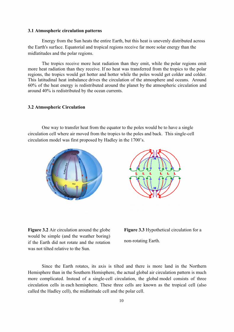
One way to transfer heat from the equator to the poles would be to have a single circulation cell where air moved from the tropics to the poles and back. This single-cell circulation model was first proposed by Hadley in the 1700’s.

Figure 3.2 Air circulation around the globe would be simple (and the weather boring) if the Earth did not rotate and the rotation was not tilted relative to the Sun.

Figure 3.3 Hypothetical circulation for a

non-rotating Earth.

Since the Earth rotates, its axis is tilted and there is more land in the Northern Hemisphere than in the Southern Hemisphere, the actual global air circulation pattern is much more complicated. Instead of a single-cell circulation, the global model consists of three circulation cells in each hemisphere. These three cells are known as the tropical cell (also called the Hadley cell), the midlatitude cell and the polar cell.

11

Main wind belts: Because the Coriolis force acts to the right of the flow (in the Northern Hemisphere), the flow around the 3-cells is deflected. This gives rise to the three main wind belts in each hemisphere at the surface: The easterly trade winds in the tropics, The prevailing westerlies, The polar easterlies

Doldrums, ITCZ: The doldrums are the region near the equator where the trade winds from each hemisphere meet. This is also where you find the intertropical convergence zone (ITCZ). It is characterized by hot, humid weather with light winds. Major tropical rain forests are found in this zone. The ITCZ migrates north in July and south in January.

Horse latitudes: The horse latitudes are the region between the trade winds and the prevailing westerlies. In this region the winds are often light or calm, and were so-named because ships would often have to throw their horses overboard due to lack of feed and water.

Polar font: The polar front lies between the polar easterlies and the prevailing westerlies.

Figure 3.4 Surface Features of the Global Atmospheric Circulation System

Pressure belts: The three-cell circulation model has the following pressure belts associated with it :

12

• Equatorial low – A region of low pressure associated with the rising air in the ITCZ. Warm air heated at the equator rises up into the atmosphere leaving a low pressure area underneath. As the air rises, clouds and rain form.

• Subtropical high – A region of high pressure associated with sinking air in the horse latitudes. Air cools and descends in the subtropics creating areas of high pressure with associated clear skies and low rainfall. The descending air is warm and dry and deserts form in these regions.

• Subpolar low – A region of low pressure associated with the polar front.

• Polar high – A high pressure region associated with the cold, dense air of the polar regions.

In reality, the winds are not steady and the pressure belts are not continuous.

Figure 3.5 "Ideal" Zonal Pressure Belts An imaginary uniform Earth with idealized zonal (continuous) pressure belts.

Figure 3.6 Actual Zonal Pressure Belts

Large landmasses disrupt the zonal pattern

breaking up the pressure zones into semi

permanent high and low pressure belts.

13

There are three main reasons for this:

• The surface of the Earth is not uniform or smooth. There is uneven heating due to land/water contrasts.

• The wind flow itself can become unstable and generate “eddies.”

• The sun doesn’t remain over the equator, but moves from 23.5oN to 23.5oS and back over the course of a year.

Figure 3.6 Earth trip around the sun through a year and seasons

3.3 Global climate

Global climate is the largest spatial scale. We are concerned with the global scale when we refer to the climate of the globe, its hemispheres, and differences between land and oceans. Energy input from the sun is largely responsible for our global climate. The solar gain is defined by the orbit of Earth around the sun and determines things like the length of seasons. The distribution of land and ocean is another import influence on the climatic characteristics of the Earth. Contrasting the climate of the Northern Hemisphere, which is approximately 39% land, with the Southern Hemisphere, which only has 19%

14

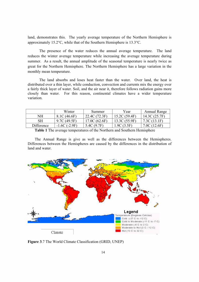
land, demonstrates this. The yearly average temperature of the Northern Hemisphere is approximately 15.2°C, while that of the Southern Hemisphere is 13.3°C.

The presence of the water reduces the annual average temperature. The land reduces the winter average temperature while increasing the average temperature during summer. As a result, the annual amplitude of the seasonal temperature is nearly twice as great for the Northern Hemisphere. The Northern Hemisphere has a large variation in the monthly mean temperature.

The land absorbs and loses heat faster than the water. Over land, the heat is distributed over a thin layer, while conduction, convection and currents mix the energy over a fairly thick layer of water. Soil, and the air near it, therefore follows radiation gains more closely than water. For this reason, continental climates have a wider temperature variation.

Winter Summer Year Annual Range NH 8.1C (46.6F) 22.4C (72.3F) 15.2C (59.4F) 14.3C (25.7F) SH 9.7C (49.5F) 17.0C (62.6F) 13.3C (55.9F) 7.3C (13.1F)

Difference -1.6C (-2.9F) 5.4C (9.7F) 1.9C (3.5F) 7.0C (12.6F) Table 1 The average temperatures of the Northern and Southern Hemisphere The Annual Range is give as well as the differences between the Hemispheres.

Differences between the Hemispheres are caused by the differences in the distribution of land and water.

Figure 3.7 The World Climate Classification (GRID, UNEP)

15

Instead, there are semi-permanent high- and low-pressure systems. They are semi-permanent because they vary in strength or position throughout the year.

Wintertime ;

• Polar highs develop over Siberia and Canada

• The Pacific High, Azores High (parts of the subtropical high pressure system) Aleutian Low and Icelandic Low form

Summertime ;

• The Azores high migrates westward and intensifies to become the Bermuda High

• The Pacific high also moves westward and intensifies

• Polar highs are replaced by low pressure

• A low pressure region forms over southern Asia

Figure 3.8 Sea level pressure and surface wind in January

16

Figure 3.9 Sea level pressure and surface wind in January

3.4 Regional climates

The major factors that determine global climate also influence climate on a regional

scale. Regional climates are influenced by water bodies and mountain ranges. Lakes exert a moderating influence on local climate, in a manner similar to how oceans affect larger climate. The Great Lakes are a good example for demonstrating the impact of lakes on climate. The Great Lakes also influence the temperature of the region. The temperature of the water is lower than the land from mid-March to August. Largest differences occur from mid-May to early June. The water temperature is greater than that of the land from late August to mid March, with the largest differences in late November and early-December in late autumn and winter. Exchanges of heat and moisture above the lakes are the key to weather modification by the Great Lakes. The influence of large water bodies on the weather of surrounding regions is most marked when the temperature differences are greatest.

Regional climates are occurs by controls in follow; • Latitude -determines solar energy input

• Elevation -influences temperature and precipitation

• Topography -Mountain barriers up wind can affect precipitation of a region as well as temperature. Topography also affects the distribution of cloud patterns and thus solar energy reaching the surface.

17

• Large bodies of water - thermal stability of water moderates the temperature of regions

• Atmospheric circulation

Large mountains influence regional climates. For example Turkey’s diverse regions have different climates because of irregular topography. Taurus Mountains is close to the coast and rain clouds cannot penetrate to the interior part of the country. Rain clouds drop most of their water on the coastal area. As rain clouds pass over the mountains and reach central Anatolia they have no significant capability to produce of rain.

Figure 3.10 The Mountain influence on Turkey precipitation

A big difference is observed when the total rainfall between coastal stations and inland stations, are compared. For example, Antalya station, located Mediterranean coast in front of the Taurus Mountain, receives greatest rainfall in the winter and its annual total is 1063 mm. On the other hand, Karaman and Burdur stations located in the back of Taurus, receive one-third amount of Antalya. Similar effect is viewed in the Black Sea Region. While the coastal Station Hopa receives 2182 mm annual rainfall, in the inland station Bayburt receives only 420 mm. In the Black sea coast, there is an orographic form of rainfall which humid air comes from over Black sea and rises through very High Mountain. When air mass became colder, it can’t carry their water content and most of the rainfalls drop in the coastal area. Therefore, the inland stations lack adequate rainfall.

18

4. Characteristics and uses of climate observations

Climate observations are important because they help satisfy important social, economic and environmental needs. They are an integral part of reducing the risk of loss of life and damage to property. Senior managers in National Meteorological and Hydrological Services (NMHSs) will need to regularly brief their governments of the reasons for recording, collecting and managing observations. Climate observations are sourced from the numerous meteorological and related observational networks and systems (Fig.4.1) that underpin applications such as weather forecasting, air pollution modelling and environmental impact assessments.

Figure 4.1 Schematic showing a variety of observation systems of relevance to National Meteorological and Hydrological Services. Observation networks rely heavily on the cooperation of many individuals and organizations, many of them volunteers. (Source: Bureau of Meteorology, Australia)

However, climate observations differ in a number of important respects. Firstly,

climate observations need to account for the full range of elements that describe the climate system – not just those that describe the atmosphere. Extensive observations of the ocean and terrestrial-based systems are required. Secondly, an observation at any point in time needs a reference climate against which it can be evaluated, i.e. a reference climatological period must be selected. In this regard, the observations from a station that only exists for a short period (i.e. from days to a few years) or which relocates very frequently will generally be of less value than those observations from a station whose records have been maintained to established standards over many years. Thus, in order to derive a satisfactory climatological average (or normal) for a particular climate element, a sufficient period record of homogeneous, continuous and good quality observations for that element is

19

required. Thirdly, a climate observation should be associated – either directly or indirectly - with a set of metadata that will provide users with information, often implicitly, on how the observation should be interpreted and used. Other differences can be inferred from the sections that follow. So, while climate observations serve multiple purposes beyond specific climate needs, we must ensure that they retain, and acquire, particular characteristics that serve a range of climate needs.

The basic monthly, seasonal and annual summaries of temperature, rainfall and

other climate elements provide an essential resource for planning endeavours in areas such as agriculture, water resources, emergency management, urban design, insurance, energy supply and demand management and construction. Climate data, including historical daily data, are also unlocking important relationships between climate and health, including the effects of extreme heat and cold on mortality. Millions of people each year use climatological information in planning their annual vacations. In a relatively new area of applications, high quality climate observations are being used by the weather derivatives industry, which has already traded billions of dollars US based to a large degree on climate information. Trenberth et al. (2002) provides several examples of the benefits of climate data. The need for more accurate analysis and detection of climate change and the promise of further advances in seasonal-to-interannual prediction (SIP) have increased the value of climate data in recent decades (Fig. 4.2).

Figure 4.2 Output from a whole-farm economic model for a farm in India showing the

cash flow benefits from using a management strategy which includes climate forecasts. As inputs to these models, climate observations have demonstrable economic benefits. (Source: H.Meinke, Queensland Department of Primary Industries)

Climate data are fundamental to the operation and validation of climate models,

which are widely used for SIP and for generating projections of future climate. Maximising the availability of computerised historical data, including metadata, is essential for long-term climate monitoring - particularly for analysing trends in the occurrence of extreme

20

events where data quality and longevity of record become even greater considerations (e.g. Nicholls 1995, Karl and Easterling 1999).

The more stringent requirements on observation networks and systems for recording

and monitoring climate, including the detection of climate change, has led to the development of special networks at national (e.g. Reference Climate Stations), regional (e.g. Regional Basic Climatological Network) and global (e.g. the Global Climate Observing System - GCOS - Surface Network, GSN) scales.

Principles of climate monitoring some guiding principles for long-term sustainable

climate monitoring have been identified and described (e.g. Karl et all. 1995, NRC 1999). While these were primarily developed for the purposes of improving our ability to detect climate change, the principles are widely applicable to all facets of climate observations. The ten principles as stated in GCOS (2003), endorsed by the Commission for Climatology (CCl) and adopted by the UNFCCC are:

1- The impact of new systems or changes to existing systems should be assessed prior to implementation:

In this context, relevant changes are those affecting instruments, observing practices, observation locations, sampling rates, etc. The pace of change in observation networks and systems has increased during the past few decades and it is very likely that this trend will continue. Many of these changes are deliberately introduced as a result of the availability of improved technology that, for example, improves observational accuracy. Providing continuity and homogeneity of climate records can be preserved, these changes are to be encouraged by climatologists, particularly if the new technology is more reliable. However, the reasons behind some changes, e.g. purely for cost savings or to solely respond to the demands of a single stakeholder, may have less justification from a climate perspective and these should prompt climatologists to question their value. Some changes, however, are unavoidable. A key consideration in the introduction of a new system is the likelihood of the system operating, and providing continuous and homogeneous observations, over the long-term. Strategies, such as a well coordinated change management program, will be required to minimise any adverse impacts from a change.

2- A suitable period of overlap for new and old observing systems is required:

Parallel observation programs between existing observation systems and their

replacements (or between new and old meteorological sites in the event of relocation) should be part of any strategy to preserve the continuity and homogeneity of the climate record. Priority should be given to those stations that are part of special networks for climate change detection. These programs may also include retrospective comparisons between former sites or old, retired observation systems where these locations and/or systems are still available for use. Observation managers may question the additional costs or overheads in conducting such parallel observations, particularly where many competing demands stretch their budgets. Climatologists must be prepared to show that benefits outweigh the costs and such endeavours are worth pursuing.

21

3- The details and history of local conditions, instruments, operating procedures, data processing algorithms and other factors pertinent to interpreting data (i.e. metadata) should be documented and treated with the same care as the data themselves:

Good quality metadata are now critical to meteorological services, particularly for

climate operations and research. There is a need for ready access to metadata (i.e. preferably in electronic form) for: data interpretation; quality control; network selection; network/system performance monitoring; client expectations; international obligations (e.g. for GCOS Surface Networks); and identification and adjustment of climate records for non-climatic discontinuities. As well as the station specific metadata, climatologists and data managers will need metadata on broader network issues, e.g. details on historical changes in calculating derived climate variables and information on changes in analysing weather systems (e.g. tropical cyclones). Unfortunately, metadata are often incomplete, poorly organised and inaccessible and this presents a major challenge for organisations. Metadata management through a modern database system (Fig. 4.3) is desirable although paper-based records will still need to be managed and preserved, including through conversion to electronic and/or microfilm/microfiche form if possible.

Figure 4.3 Modern databases are providing efficient access to important station metadata, including photographs, site plans and other useful documents. (Source: Central Institute of Meteorology and Geodynamics ZAMG, Austria)

Recording of information in spreadsheets may be a useful interim way of ensuring

that metadata are maintained. Management of metadata should fit with the broader information policy of an organisation and must ensure that private (e.g. observer addresses), personal (e.g. performance information) and any commercial-in-confidence information are not distributed without approval or consent.

4- The quality and homogeneity of data should be regularly assessed as a part of routine operations:

It is important that the responsibilities for ensuring the quality of climate data are

distributed throughout the organisation and are not considered the sole responsibility of climate data managers. Meteorological services should endeavour to develop a Data

22

Management policy with strategies that involve a strong focus on data quality, and including laboratory and testing facilities, quality assurance processes, real-time monitoring and correction, quality control procedures and data archiving. Some organisations may extend this philosophy to a quality policy for the organisation (e.g. Knez et al. 2003). The monitoring principles 1 to 3 discuss ways of minimising the impacts of inhomogeneities. Organisations should also endeavour to have systems in place to alert to inhomogeneities in near real-time so that early corrective action can be taken. So far, delayed-mode detection of inhomogeneities has most commonly been applied to temperature and precipitation data. Adjusting for inhomogeneities has proven more problematic for some climate elements (e.g. dew point, wind speed and direction).

4.5 Consideration of the needs for environmental and climate-monitoring products and assessments, such as assessments from the Intergovernmental Panel on Climate Change (IPCC), should be integrated into national, regional and global observing priorities:

Climatologists need to identify the observational priorities for their countries based

on the capabilities of existing networks and systems to satisfy a range of climate needs. As well as quality requirements, climatologists should ensure that networks provide adequate spatial and temporal sampling so that areas that exhibit large spatial variations in climate are adequately sampled and that areas that experience (or which may be expected to in the future) large temporal or spatial climatic variations are also well sampled. In addition to the recommendations from reports of the IPCC, the adequacy of observation networks and systems at large regional and global levels are assessed by the GCOS adequacy reports for the UNFCCC (GCOS 1998, GCOS 2003) and their recommendations should be integrated into national priorities. Many countries prepare national reports on their systematic climate observations as a result of requests from the UNFCCC Conference of the Parties (COP) and these too should be utilised. Another important aspect of this monitoring principle is to anticipate the use of observations in the development of environmental impact assessments. In this respect, co-location of priority climate stations with sensors monitoring wider atmospheric parameters (e.g. the Global Atmospheric Watch Network monitoring atmospheric constituents, see Fig.4.4) should be given strong consideration.

23

Figure 4.4 The Cape Grim Baseline Air Pollution Station on the remote north-western tip of Tasmania (Australia) samples air flowing from the Southern Ocean, largely free from athropogenic pollutants. (Source: Bureau of Meteorology, Australia)

6- Operation of historically-uninterrupted stations and observing systems should be maintained. This principle is another that is fundamental to the production of homogeneous and continuous climate records:

Countries have been encouraged to identify stations in a number of special networks established for long-term climate monitoring, which will help satisfy this goal. However, the desire for continuous operation should permeate throughout all meteorological and related station networks that provide climatological data. Since changes in observing systems are inevitable, it is critical that NMHSs have change management programs in place, which include parallel observation programs. Much effort is being channelled into ensuring the long-term continuation of sites critical to climate (Fig. 4.5). Countries should recognise that their stations with long historical time series of climatological elements constitute national, regional and global heritage to their nations.

24

Figure 4.5 An example of a long and valuable climate data series. The Central England Temperature (CET) is representative of a roughly triangular area of the United Kingdom enclosed by Bristol, Manchester and London. The monthly series began in 1659, and to date is the longest available instrumental record of temperature in the world. Since 1974 the data have been adjusted by 1-2 tenths °C to allow for urban warming. (Source: The Hadley Centre, United Kingdom Meteorological Office)

7- High priority for additional observations should be focussed on data-poor regions, poorly-observed parameters, regions sensitive to change, and key measurements with inadequate temporal resolution:

National, regional and global network adequacy assessments are pertinent here. The

development of improved observational technologies should focus on those observations and regions for which capturing quality observations have proven problematic (e.g. precipitation in cold climates). Often these regions are associated with ecosystems that are sensitive to climate change and so the observations have additional importance for climate impacts assessments and adaptation studies. Priorities should also be linked to the social, economic and environmental fabric of the country and this may, for example, strengthen the case for supporting the observational needs for specific climate applications. The GCOS and Reference Climate Station (RCS) networks may have inadequate spatial resolution for monitoring some critical climate elements at the national scale (e.g. precipitation) so that

25

some additional national networks, which adhere to these climate monitoring principles, will need to be identified.

8- Long-term requirements, including appropriate sampling frequencies, should be specified to network designers, operators and instrument engineers at the outset of system design and implementation:

Sustainable climate monitoring can only be achieved through a shared

understanding, and considerable liaison, between observation network and system managers, data managers and climatologists. The latter will need to represent the very broad needs of end-users. There are close parallels here with the first principle identified, particularly regarding the need for a change management program. There are some good examples of countries who have attempted to seek all stakeholder needs, including climatological needs, prior to designing new networks (e.g. Frei 2003). Climatologists should be ready to respond to demands for this information by attempting to provide details of national observation needs for a range of key climatological applications (e.g. analysis of climate variability, climate prediction) and, with respect to individual climate elements, requirements for quality, spatial density and sampling frequency.

9- The conversion of research observing systems to long-term operations in a carefully-planned manner should be promoted:

The needs of climate imply a long-term commitment to observing systems is

required. For those systems that have potential for climate monitoring, there needs to be a clear transition plan (from research to operations) developed. Some of the best examples of observation networks and systems that have made the transition are the Tropical Atmosphere Ocean (TAO) array established as part of the Tropical Ocean Global Atmosphere (TOGA) experiment for monitoring the El Nino-Southern Oscillation phenomenon. Any transition will require the development of infrastructure supporting the broader requirements of climate as described elsewhere in this section (e.g. metadata, robust data management systems, regular maintenance/inspection of stations, life-cycle management of equipment and sensors).

10- Data management systems that facilitate access, use and interpretation of data and products should be included as essential elements of climate monitoring systems:

One of the major differences between the observational requirements of climate and

weather concerns the treatment of observations beyond a few hours of their collection. While the operational value of observations to weather forecasters usually rapidly depreciates, it does not for climatologists. Climate data management systems generally sit between the observation systems and the delivery and production of climate products and services (Fig. 4.6).

26

Figure 4.6 The fundamental role of observations, networks, climate data management systems and metadata in providing climate information. (Source: Bureau of Meteorology, Australia).

They include the quality control systems, metadata and various feedbacks between

data users and observation system and network managers that help preserve the integrity of the climate data. A robust and secure climate database is the cornerstone to the development and delivery of good quality products and services. Organisations should strive to develop a data management policy that secures data on paper-based records as well as those collected by more direct means.

While much of the above concerns the need for climatologists to ensure the stability

of climate observations they must also look at the opportunities presented by observation systems particularly with regard to new data types, including high resolution observations (Fig. 4.7).

27

Figure 4.7 Increasing the observation frequency of highly variable elements such as wind speed improves the calculation of climate statistics such as the annual mean. (Source: Muirhead 2000)

Future use of these observations could effectively remove the limitations of having

to derive daily means from hourly or daily observations and could also be used to derive new variables (e.g. climatologies of rapid changes).

In-Situ Climatological Observations and Instruments

Remote sensing observations

Satellite based climate products

Top of Atmosphere Albedo (TOA) Solar Incoming Radiation Surface (SIS) Cloud Fractional Cover (CFC) Humidity Composit Product (HCP)

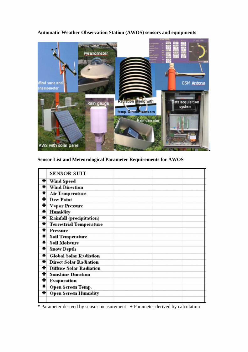
Automatic Weather Observation Station (AWOS) sensors and equipments

Sensor List and Meteorological Parameter Requirements for AWOS

* Parameter derived by sensor measurement + Parameter derived by calculation

28

5. VEGETATION Vegetation also affects regional climate an observation made obvious when comparing

the wind speed within a forest with the wind speed at the same height over an open field. Friction reduces the wind speed in the forest, so open areas have greater winds. The relative humidity is usually greater in a forest than in the surrounding open country. Forests depress the summer temperatures by 1 to 2 C (2-4F) below the annual mean in their vicinity. This temperature difference is driven by heat budget differences; less solar energy reaches the forest floor than the open field.

Figure 5 World vegetation map (GRID, UNEP)

6. PALEOCLIMATOLOGY - DETERMINING PAST CLIMATES A fuller understanding of past climates enables scientists to better predict future

climate, including the impact of humans. Uncovering the global and regional climates of the past is like a solving a mystery. We look for evidence and compile this evidence into a consistent story. Paleoclimatology is the study of climate and climate change throughout geologic time. This section discusses some of the methods paleoclimatologists use to collect evidence. Paleoclimatology is the study of ancient climates

29

6.1. How do we reconstruct climate?

• Tree Rings • Glacial Ice Cores • Ocean Sediments - The ratio of

oxygen 16 to oxygen 18 preserved in the steady rain of dead organisms.

• Radiocarbon dates of organic material

• Pollen samples found in packrat middens and lake bed samples.

• Variations in desert varnish coatings found on rocks in the arid southwest

• Variations found in peatbog deposits

• Sedimentary rock records. Figure 6.1 NOAA paleoclimatology web site

http://www.ncdc.noaa.gov/paleo/paleo.html 6.2. Tree Rings

• How does a tree produce annual rings? • There are two main types of ring producing trees.

The primary cellular component of tree rings is the tracheid. Tracheids are long tubular cells that make up the xylem. Tracheids formed in the beginning of the growing season are thin walled and low in density. These cells constitute what is called the earlywood. As the end of the growing season nears, climate conditions become less conducive and growth slows. Tracheids become darker and more thick-walled, forming the latewood. Finally, when the growth season ends, there is a marked boundary at the edge of the ring.

Figure 6.2 Cross section of a conifer 6.3. Dendrochronology (tree-ring dating)

Dendrochronology is the study of tree rings and is derived from the Greek words for tree and knowing the time.

Simply stated, trees grow two rings per calendrical year. For the entire period of a

tree's life, a year-by-year record or ring pattern is formed that in some way reflects the climatic conditions in which the tree grew. These patterns can be compared and matched ring for ring with trees growing in the same geographical zone and under similar climatic conditions. Following these tree-ring patterns--the sum of which refer to as chronologies--

30

from living trees back through time, it can thus compare wood from old or ancient structures to our known chronologies, match the ring patterns (cross-dating), and determine precisely the age of the wood used by the ancient builder.

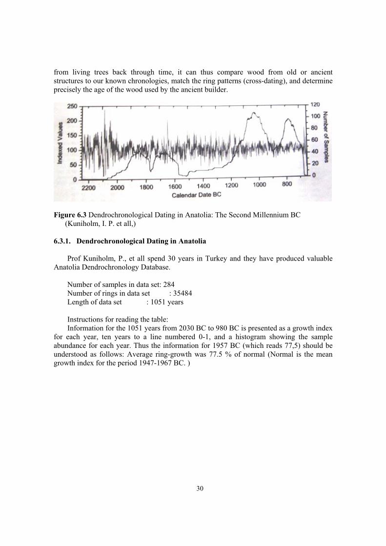
Figure 6.3 Dendrochronological Dating in Anatolia: The Second Millennium BC (Kuniholm, I. P. et all,) 6.3.1. Dendrochronological Dating in Anatolia

Prof Kuniholm, P., et all spend 30 years in Turkey and they have produced valuable

Anatolia Dendrochronology Database.

Number of samples in data set: 284 Number of rings in data set : 35484 Length of data set : 1051 years Instructions for reading the table: Information for the 1051 years from 2030 BC to 980 BC is presented as a growth index

for each year, ten years to a line numbered 0-1, and a histogram showing the sample abundance for each year. Thus the information for 1957 BC (which reads 77,5) should be understood as follows: Average ring-growth was 77.5 % of normal (Normal is the mean growth index for the period 1947-1967 BC. )

31

Table 2. Bronze / Iron Age Master Chronology for the Second Millennium BCTree-Growth Indices for the Second Millennium BC Number of Samples per YearDate 0 9 8 7 6 5 4 3 2 1 0 9 8 7 6 5 4 3 2 1

-2030 91.5 51.0 99.2 130.7 114.6 127.2 87.4 114.4 122.0 122.2 10 10 10 10 10 10 10 10 10 11-2020 97.4 121.0 81.9 79.0 61.0 122.4 95.7 64.6 104.0 129.5 11 11 11 11 11 11 11 11 13 13-2010 107.0 103.8 130.6 111.5 100.7 118.6 83.9 138.3 104.3 86.1 13 14 14 15 15 16 17 17 17 17-2000 109.3 91.3 102.8 95.5 96.7 122.3 111.1 90.3 110.2 81.6 17 17 17 17 17 17 17 17 17 16-1990 114.6 101.0 93.3 90.5 103.3 66.3 76.3 76.7 76.3 80.0 16 16 16 16 16 16 16 16 16 15-1980 97.9 96.9 87.6 95.7 73.5 89.8 83.2 84.9 81.0 99.0 15 15 15 15 15 16 16 16 16 16-1970 85.4 127.0 130.9 106.0 78.0 89.9 114.3 79.1 108.7 107.1 17 17 17 18 18 18 18 18 18 18-1960 97.0 111.8 107.9 77.5 104.4 115.5 109.1 129.7 121.2 83.7 18 18 18 18 18 18 18 18 18 18-1950 76.6 64.1 84.0 88.6 91.9 95.7 85.8 99.9 65.4 98.4 18 18 18 18 19 19 19 19 18 18-1940 108.6 109.5 83.8 73.8 96.1 109.9 81.5 97.1 102.5 128.3 19 19 20 20 20 21 21 21 21 21-1930 111.8 95.6 93.7 113.9 124.8 92.7 106.7 85.8 118.2 109.0 20 21 23 24 26 26 26 27 28 28-1920 93.8 70.7 103.7 125.3 127.4 127.2 129.4 101.3 123.2 133.6 28 29 29 29 29 30 30 31 31 31-1910 124.8 108.8 78.6 131.5 100.9 120.2 111.7 109.9 130.2 124.3 32 32 32 32 33 34 34 34 35 36-1900 128.1 102.8 131.2 104.3 108.4 82.6 110.3 92.1 101.2 72.5 36 36 36 36 36 36 35 35 35 35-1890 104.9 89.2 123.9 115.7 110.9 100.0 102.1 111.4 91.4 91.8 35 35 35 36 37 38 38 37 37 37-1880 101.5 100.6 89.1 91.0 93.1 92.3 92.3 91.9 70.4 89.6 37 37 37 37 37 37 38 38 38 38-1870 99.7 82.2 71.4 101.3 87.2 92.3 91.8 91.3 104.2 117.9 38 38 38 38 38 39 39 39 40 40-1860 109.4 123.3 116.7 97.0 110.9 116.8 86.3 100.5 114.2 66.7 40 40 40 39 38 39 39 41 41 42-1850 82.2 88.3 112.1 121.9 115.3 108.8 121.8 108.1 100.7 82.1 41 40 40 41 42 43 43 43 46 46-1840 78.9 77.9 91.6 89.7 64.7 94.1 100.1 99.4 93.3 115.1 47 49 49 50 50 48 49 48 45 40-1830 106.7 120.0 129.5 104.1 83.7 97.1 110.5 118.2 110.1 69.9 40 40 40 40 39 39 39 39 39 38-1820 84.6 104.9 95.1 115.4 101.3 104.7 81.6 107.1 102.7 95.8 38 38 38 37 37 37 37 37 37 37-1810 113.8 119.2 101.5 84.2 117.0 86.3 86.5 128.0 112.1 113.6 37 36 36 36 36 36 35 35 35 35-1800 128.3 98.8 52.1 88.5 110.1 121.6 93.4 110.7 76.7 76.8 36 36 37 36 37 36 36 35 34 34-1790 97.4 83.0 89.5 79.8 76.0 99.5 81.9 105.6 89.5 117.5 34 34 34 34 34 35 35 35 34 32-1780 105.2 112.1 109.9 116.8 110.7 112.4 74.8 75.0 71.5 74.1 32 31 31 31 30 28 23 15 14 14-1770 81.5 55.9 75.0 90.8 104.5 137.0 93.7 105.8 83.4 133.1 14 14 13 13 14 15 15 16 16 16-1760 117.8 128.1 116.0 95.8 148.3 94.2 105.3 98.5 123.0 148.7 16 16 16 16 17 17 18 19 19 20-1750 146.1 104.5 106.3 130.1 109.4 119.3 105.9 128.0 110.1 114.8 22 24 26 27 27 27 28 29 30 31-1740 106.2 98.1 101.8 98.8 81.5 117.3 111.3 70.5 89.6 86.1 31 31 31 31 32 33 36 37 37 37-1730 102.7 97.1 74.6 72.4 72.0 96.4 103.4 116.4 120.4 86.3 37 37 37 37 37 37 37 37 37 38-1720 126.2 132.5 71.5 101.4 115.4 141.5 127.0 114.3 102.0 114.0 38 39 39 39 38 38 38 38 38 37-1710 106.2 95.9 86.8 98.7 95.3 90.2 84.2 66.1 90.1 73.7 36 35 35 35 36 36 36 36 36 36-1700 84.3 35.0 105.2 65.5 63.8 90.4 88.3 92.9 92.1 81.7 36 36 36 37 40 40 40 40 40 40-1690 99.6 116.5 134.9 120.0 116.7 120.0 107.5 66.4 110.7 113.7 41 41 41 40 41 41 41 41 41 41-1680 105.4 95.5 65.2 74.6 92.0 101.5 112.5 121.5 146.6 130.7 40 40 40 40 40 39 39 40 42 42-1670 57.8 52.2 101.2 102.1 75.8 98.8 53.8 92.4 90.7 65.0 42 42 42 41 41 40 40 40 40 40-1660 94.0 111.1 110.9 121.7 117.1 83.4 101.6 83.8 56.8 52.4 40 40 40 41 41 41 41 41 41 40-1650 120.2 165.6 207.0 184.2 167.4 155.0 124.3 99.8 132.2 114.3 40 40 40 40 40 40 39 38 36 36-1640 118.7 139.8 119.4 93.3 95.3 79.7 88.0 97.9 78.5 71.9 36 36 36 36 36 37 36 35 35 34-1630 61.4 89.5 89.1 86.1 97.7 115.6 133.2 127.0 92.6 105.0 34 34 33 33 33 33 33 33 33 33-1620 108.3 100.3 108.3 81.4 90.4 54.5 69.9 111.9 59.2 107.4 32 32 31 31 31 31 31 31 30 30-1610 80.8 75.5 99.3 112.0 117.6 105.2 89.5 89.7 88.4 86.6 31 31 31 31 31 31 30 28 28 28-1600 90.8 92.9 76.5 96.2 108.6 131.8 95.1 91.0 83.1 92.7 29 29 28 28 28 27 27 27 26 26-1590 90.6 122.5 83.2 113.5 90.6 109.5 125.6 59.6 79.8 99.5 26 26 26 26 26 25 24 24 24 24-1580 129.8 89.7 132.0 148.0 140.8 117.8 98.4 109.5 90.5 96.7 24 24 24 23 21 21 17 10 7 7-1570 102.2 108.8 79.3 84.1 134.6 133.6 119.2 94.0 80.8 64.4 7 7 7 7 7 6 6 6 6 6-1560 95.1 110.2 76.8 58.8 105.1 120.7 68.2 73.3 75.9 79.0 6 6 6 6 6 6 6 6 6 6-1550 108.5 99.2 70.6 47.1 75.0 119.0 92.6 100.2 69.2 85.8 6 6 5 5 5 5 5 5 5 5-1540 89.9 121.4 110.6 120.1 120.2 97.1 98.0 93.8 85.6 58.5 5 5 5 5 5 5 5 5 5 5-1530 116.6 131.8 62.6 123.8 126.4 101.1 80.7 67.3 71.9 76.1 5 5 5 5 5 5 5 5 4 4-1520 80.7 55.5 115.1 119.4 103.2 86.7 119.0 103.6 107.8 108.0 4 4 4 4 4 5 5 5 5 6-1510 147.3 139.0 95.5 167.9 121.6 132.9 131.4 124.3 120.2 96.1 6 6 6 6 6 8 10 10 10 10-1500 130.1 137.3 121.3 100.9 153.0 136.0 78.6 110.5 137.2 127.6 11 11 11 11 11 11 12 12 12 12-1490 127.1 85.5 86.7 89.9 76.2 61.6 63.9 98.3 77.8 100.8 12 12 12 12 12 12 12 12 12 12-1480 82.0 120.5 100.3 74.6 88.5 117.3 94.7 108.8 77.0 87.3 12 12 12 12 11 11 11 11 11 11-1470 66.1 100.5 98.0 90.3 144.2 112.1 97.5 117.2 63.5 155.4 11 11 11 11 11 11 11 11 11 11-1460 159.5 99.2 107.7 150.4 111.6 68.8 73.6 116.2 119.0 109.2 11 11 11 12 12 12 12 12 12 12-1450 105.0 147.8 113.3 93.2 99.3 115.3 154.2 125.3 130.4 99.2 13 13 13 13 13 13 13 13 13 13-1440 104.6 110.6 103.3 86.4 91.9 72.5 83.9 112.5 76.2 76.9 13 13 13 13 13 13 13 13 13 13-1430 112.0 108.2 116.2 123.1 123.7 81.5 120.8 115.4 79.6 81.6 13 13 13 13 13 13 13 13 13 13-1420 114.0 80.7 106.2 151.9 106.8 42.1 89.1 104.2 143.1 127.0 13 13 13 13 13 13 13 13 13 13-1410 121.2 76.4 104.6 109.5 77.1 107.1 95.6 105.9 97.4 76.0 13 13 13 13 13 13 13 13 13 13-1400 101.8 77.4 106.1 84.1 68.8 92.3 122.4 94.4 116.9 97.7 13 13 13 13 13 13 13 13 13 13-1390 112.3 73.8 54.5 72.0 85.6 118.3 74.0 116.7 145.8 147.8 13 13 13 13 13 13 13 13 13 13-1380 145.0 127.0 129.3 118.3 74.1 98.5 116.8 73.0 81.0 106.1 13 13 13 13 13 13 13 13 13 13-1370 93.5 104.7 115.9 112.4 86.8 81.9 127.5 102.7 119.6 123.5 13 13 13 13 13 13 13 13 13 14-1360 110.2 114.7 87.7 39.7 99.1 86.0 117.4 85.0 67.3 109.7 14 14 14 14 14 14 14 14 14 14-1350 70.5 47.8 81.1 116.3 147.2 117.1 101.6 72.8 93.9 76.9 14 14 14 14 14 14 14 14 14 14-1340 159.5 144.8 133.2 108.4 89.2 89.6 109.0 75.6 67.1 101.6 14 14 14 14 14 14 14 15 15 15-1330 54.0 94.8 85.4 115.7 107.2 58.3 99.2 93.6 104.5 126.2 15 15 15 15 16 16 16 16 16 16-1320 99.1 78.2 72.5 76.8 95.4 96.6 74.8 63.0 106.5 68.4 17 17 17 17 17 17 17 17 17 17-1310 99.1 138.3 127.3 90.5 95.2 111.1 117.1 172.2 83.1 115.6 17 17 17 17 17 17 17 17 17 17

Perio

d of

N

orm

al

32

-1300 114.4 130.9 124.2 113.9 116.7 97.2 91.7 93.4 111.0 80.3 17 17 17 17 17 17 17 17 17 17-1290 99.9 102.0 79.5 45.4 62.0 104.4 146.1 141.1 124.8 86.3 17 17 17 17 17 17 17 17 17 17-1280 94.0 82.1 71.7 95.4 67.1 80.6 99.8 106.4 79.0 112.0 17 17 17 17 17 17 17 17 17 17-1270 87.4 92.5 51.5 124.1 60.2 59.4 71.5 82.0 99.4 91.2 17 17 17 17 17 17 17 17 17 17-1260 114.5 114.9 148.9 74.5 95.7 85.6 69.8 122.8 111.2 93.6 18 18 18 18 18 19 19 19 19 19-1250 130.5 133.0 118.0 103.2 76.3 99.3 111.6 95.4 125.5 98.7 20 20 20 20 20 20 20 21 20 21-1240 102.8 81.8 62.6 88.7 73.7 117.7 87.7 123.2 71.5 90.3 21 21 21 21 21 21 21 22 22 22-1230 89.5 59.3 65.5 96.7 81.9 98.2 85.1 110.7 76.1 96.9 22 22 22 22 23 24 24 24 24 25-1220 124.6 98.1 98.9 117.6 114.1 151.5 54.7 77.7 107.4 85.3 25 25 25 25 25 25 25 25 25 25-1210 119.1 101.0 149.2 135.4 119.0 107.8 150.0 169.2 137.3 123.2 25 25 25 25 26 26 26 26 25 25-1200 123.3 115.2 109.0 82.1 83.5 91.5 101.1 99.7 105.8 99.0 25 27 27 27 27 29 29 30 30 30-1190 53.5 61.1 62.0 102.3 85.8 80.3 84.2 103.6 106.4 73.6 30 30 30 31 31 33 33 34 35 35-1180 78.0 80.0 109.9 95.6 73.8 100.8 149.1 134.6 155.2 128.9 35 35 34 36 37 37 36 36 36 37-1170 73.3 77.9 137.1 115.4 125.4 139.5 114.5 145.0 124.6 98.2 38 39 40 42 42 43 44 45 45 45-1160 78.4 109.8 95.0 84.6 100.8 97.6 111.4 80.6 104.5 72.2 46 46 47 47 47 48 49 49 50 50-1150 88.2 91.0 67.6 95.3 112.7 88.6 118.4 97.6 70.5 76.9 52 52 54 54 54 54 55 57 57 56-1140 92.1 116.5 127.5 148.4 114.4 138.4 121.4 104.4 127.6 123.1 56 57 57 56 57 58 58 58 58 60-1130 119.1 126.2 114.1 85.3 128.5 111.9 99.6 79.1 85.2 81.2 61 59 59 58 58 59 59 60 62 62-1120 112.7 112.5 108.9 71.7 104.5 106.8 109.2 123.0 103.8 65.7 62 62 63 62 61 61 61 61 61 61-1110 102.6 112.5 109.0 83.6 96.3 80.9 109.1 63.2 71.2 81.3 62 63 63 63 65 65 67 69 70 72-1100 105.4 81.9 97.9 88.9 106.0 95.7 117.2 65.9 61.2 95.3 72 73 73 74 75 77 77 77 78 79-1090 120.2 104.5 106.6 110.3 70.4 127.7 89.0 99.5 811.0 77.3 80 82 83 83 84 85 86 89 90 90-1080 96.9 103.5 114.9 122.6 112.5 93.8 93.0 95.8 88.4 92.6 91 95 96 96 96 97 98 98 96 97-1070 97.1 101.2 101.5 123.8 72.3 98.8 100.2 103.5 105.0 98.6 99 99 98 97 97 96 96 96 97 98-1060 101.6 85.3 104.4 71.1 72.8 84.2 69.5 111.2 115.3 89.4 98 99 98 98 98 98 98 98 99 100-1050 98.4 102.6 118.0 111.6 87.6 96.8 121.2 126.4 115.6 89.7 101 99 98 99 98 100 103 104 104 105-1040 108.1 108.3 95.1 97.0 88.3 89.7 102.6 99.3 106.3 90.3 106 106 106 108 108 108 108 108 108 108-1030 95.4 118.7 117.8 111.7 106.6 113.3 124.7 86.4 105.1 101.0 108 107 109 106 106 107 108 107 108 106-1020 106.0 105.0 105.9 74.8 71.9 100.4 99.5 102.6 113.4 101.7 105 107 106 105 104 104 103 103 103 102-1010 99.4 104.7 116.6 117.4 115.8 75.4 104.9 108.0 119.6 108.6 102 102 102 102 101 100 100 100 101 101-1000 72.1 93.8 82.9 127.5 108.4 102.3 110.6 129.7 93.2 123.1 100 100 99 99 100 100 100 101 101 101

-990 125.5 101.0 97.6 119.5 126.7 85.6 83.6 103.0 108.9 114.2 101 100 100 97 97 97 95 92 90 90-980 103.8 90

Figure 6.4 Dendrochronology of Anatolia (Kuniholm, I. P. et all,)

Figure 6.5 Mediterranean paleo database (NCDC web site)

33

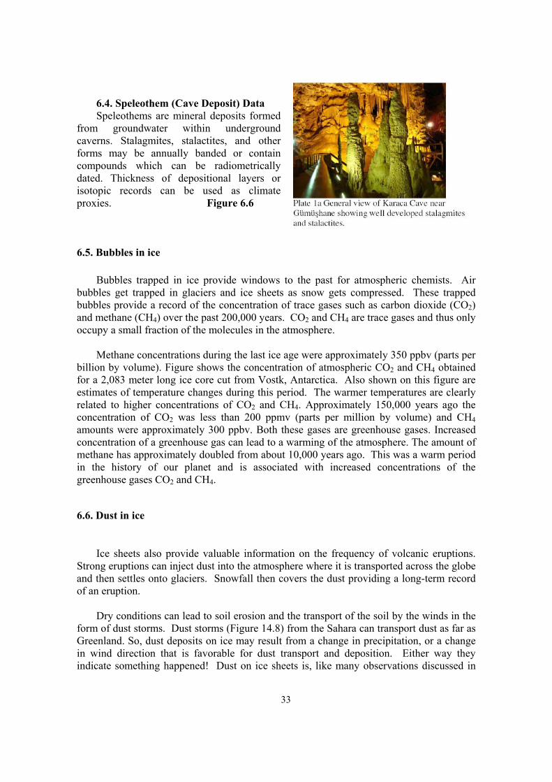
6.4. Speleothem (Cave Deposit) Data Speleothems are mineral deposits formed

from groundwater within underground caverns. Stalagmites, stalactites, and other forms may be annually banded or contain compounds which can be radiometrically dated. Thickness of depositional layers or isotopic records can be used as climate proxies. Figure 6.6

6.5. Bubbles in ice Bubbles trapped in ice provide windows to the past for atmospheric chemists. Air

bubbles get trapped in glaciers and ice sheets as snow gets compressed. These trapped bubbles provide a record of the concentration of trace gases such as carbon dioxide (CO2) and methane (CH4) over the past 200,000 years. CO2 and CH4 are trace gases and thus only occupy a small fraction of the molecules in the atmosphere.

Methane concentrations during the last ice age were approximately 350 ppbv (parts per

billion by volume). Figure shows the concentration of atmospheric CO2 and CH4 obtained for a 2,083 meter long ice core cut from Vostk, Antarctica. Also shown on this figure are estimates of temperature changes during this period. The warmer temperatures are clearly related to higher concentrations of CO2 and CH4. Approximately 150,000 years ago the concentration of CO2 was less than 200 ppmv (parts per million by volume) and CH4 amounts were approximately 300 ppbv. Both these gases are greenhouse gases. Increased concentration of a greenhouse gas can lead to a warming of the atmosphere. The amount of methane has approximately doubled from about 10,000 years ago. This was a warm period in the history of our planet and is associated with increased concentrations of the greenhouse gases CO2 and CH4.

6.6. Dust in ice

Ice sheets also provide valuable information on the frequency of volcanic eruptions. Strong eruptions can inject dust into the atmosphere where it is transported across the globe and then settles onto glaciers. Snowfall then covers the dust providing a long-term record of an eruption.

Dry conditions can lead to soil erosion and the transport of the soil by the winds in the

form of dust storms. Dust storms (Figure 14.8) from the Sahara can transport dust as far as Greenland. So, dust deposits on ice may result from a change in precipitation, or a change in wind direction that is favorable for dust transport and deposition. Either way they indicate something happened! Dust on ice sheets is, like many observations discussed in

34

this section, a piece of the climate puzzle, not the complete answer. Sediments on the ocean floor provide another clue to past climates.

6.7. Sediments Materials have been deposited in layers (Figure 14.9) on the ocean floor for very long

periods of time. The deeper the layer, the older the material. These deposits can include soil from wind erosion, soil from floods, ash from volcanic eruptions, and shells of animals. In ocean sediments, the shells of animals are primarily calcium carbonate (CaCO3), a compound that makes up limestone. The calcium carbonate is very useful for tracking past climates by the relative amounts of different oxygen isotopes.

Most oxygen atoms have an atomic weight of 16. This atomic oxygen is denoted as

16O. An oxygen atom can also have 2 additional neutrons, resulting in an atomic weight of 18 (18O). 16O is much more common than 18O. Water molecules (H2O) can incorporate both of these isotopes. So, these two isotopes of oxygen are found in ocean water and in the shells and bones of plankton. The ratio of 18O to 16O (18O/16O) provides the clue to past climates.

Foraminifera are microorganisms that live in the oceans and have hard shells of

calcium-containing compounds, including calcium carbonate. The relative amount of the two isotopes 18O to 16O in the shells of these marine protozoans is related to the amount of continental ice. The proportion of 18O to 16O is partly controlled by the volume of water in continental ice sheets. Since 16O is lighter than 18O, it can evaporate from the water more quickly. The lighter water molecule tends to accumulate as snow and ice that form the glaciers. As the ice accumulates, more of the 16O is bound in the ice sheets. So, during glacial times there is a higher concentration of 18O in the water. As foraminifera construct their shells they incorporate larger amounts of 18O than 16O because of its relative abundance. So, as continental glaciers grow, there is less 16O in the oceans leaving higher ratios of 18O/16O in the oceans and thus in the shells. As the foraminifers die, their shells settle on the ocean floor and provide a record of the isotope ratio. When we pull sediment cores from the ocean floor, we can obtain a record of the past 2 to 3 million years! These cores have indicated a variation in the growth and shrinkage of ice sheets on repetitive time cycles of 100,000, 41,000 and 20,000 years. Figure 14.10 shows the departures from the average 18O/16O ratio over the past 300,000 years. Note that warm periods occur approximately every 100,000 years.

6.8. Fossil records

Fossils provide useful records into the past. They provide a means to track life through the ages because they are an integral part of the rocks in which they are found. The age of the rocks can be dated. Fossils reveal ancient animal and plant life that can be used to infer climate characteristics of the past. For example, tropical plants often have pointed tips so that the moisture can drip off the leaf. Plant fossils that have pointed leaves indicate a

35

moist tropical climate. Large numbers of a given fossil also indicate favorable climate conditions for these organisms.

6.9. Water erosion

Moving water, whether liquid or solid as in glaciers, leaves evidence of its movement. When a cold global climate warms, glaciers recede, leaving behind geological evidence of their former presence. As they advance during cold climates, glaciers will leave scratches in hard rocks and smooth softer rocks. As a glacier advances it pushes rocks of all sizes much like a bulldozer. When it recedes, the rocks get left behind marking the glacier boundaries. Called moraines, these rock deposits are recognized by the wide assortment of rock sizes⎯from clay to boulders. Moraines are even found in eastern South America and in Africa south of the equator, indicating that these regions were once cold.

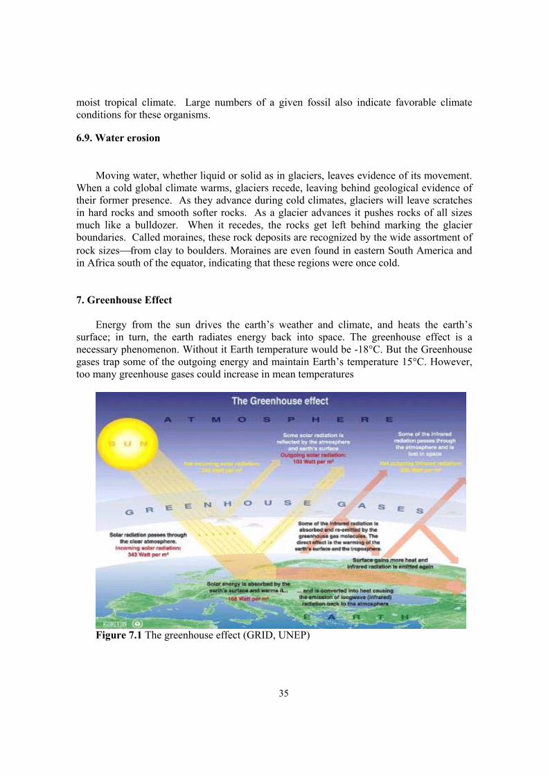
7. Greenhouse Effect Energy from the sun drives the earth’s weather and climate, and heats the earth’s

surface; in turn, the earth radiates energy back into space. The greenhouse effect is a necessary phenomenon. Without it Earth temperature would be -18°C. But the Greenhouse gases trap some of the outgoing energy and maintain Earth’s temperature 15°C. However, too many greenhouse gases could increase in mean temperatures

Figure 7.1 The greenhouse effect (GRID, UNEP)

36

Figure 7.2 Transparent and greenhouse gases Radiative flux balance

Figure 7.3 Radiative flux balance formula 8. Climate Change: In addition to the observed natural climate variability; it is changes in climate due to

anthropogenic contribution to the atmosphere (UNFCCC). Technically climate change is usually characterized by a shift in means.

Figure 8.1 Shift in mean and CO2 concentration over time

Small changes in mean can cause more extreme event. The pre industrial levels of CO2 approximately 280 ppm would then double by the end of the next century.

without greenhouse effect with greenhouse effect

37

Figure 8.2 Past, present and future climate

Figure 8.3 Observed changes in climate

38

When weather patterns for an area change in one direction over long periods of time, they can result in a net climate change for that area. The key concept in climate change is time. Natural changes in climate usually occur over; that is to say they occur over such long periods of time that they are often not noticed within several human lifetimes. This gradual nature of the changes in climate enables the plants, animals, and Microorganisms on earth to evolve and adapt to the new temperatures, precipitation patterns, etc. The real threat of climate change lies in how rapidly the change occurs. Increasing concentrations of greenhouse gases are likely to accelerate the rate of climate change.

8.1. Potential Climate Change impact

Scientists expect that the average global surface temperature could rise 0.6-2.5°C in the next fifty years, and 1.4-5.8°C (IPCC TAR, 2001) in the next century, with significant regional variation. Evaporation will increase as the climate warms, which will increase average global precipitation. Soil moisture is likely to decline in many regions, and intense rainstorms are likely to become more frequent. Sea level is likely to rise two feet along most of the U.S. coast. Calculations of climate change for specific areas are much less reliable than

Figure 8.4 Potential Climate Change impact global ones, and it is unclear whether regional climate will become more variable.

39

9. Climatological Applications 9.1. Climate Change Detection, Monitoring - Climate Indices A joint WMO CCl/CLIVAR Expert Team on Climate Change Detection, Monitoring

and Indices was tryed to detect climate change via software which prepared by Xuebin Zhang of Environment Canada. This software package, called RClimDex, uses the free software R (see http://www.r-project.org for more information). The complete list of the 27 indices, software and users guide of RClimDex are available from http://cccma.seos.uvic.ca/ETCCDMI

Figure 9.1 Rclimdex software and its outputs (27 climate indices)

40

This software is using daily precipitation, maximum and minimum temperature. If we reconstruct of past climate data, it will be possible to run RClimDex software to produce climate indices and to detect climate change from historic time to the present. One study has undertaken for the Middle East and published at: http://www.agu.org/pubs/crossref/2005/2005JD006181.shtml

Figure 9.2 Indices plot Kendall’s tau based slope estimator has been used to compute the trends since this

method doesn’t assume a distribution for the residuals and is robust to the effect of outliers in the series. If slope error greater than slope estimate we can’t trust slope estimate. If PValue is less than 0.05 this trend is significant at 95% level of confidence this indices show that frost days will be decreasing 26.8 days in 100 years.

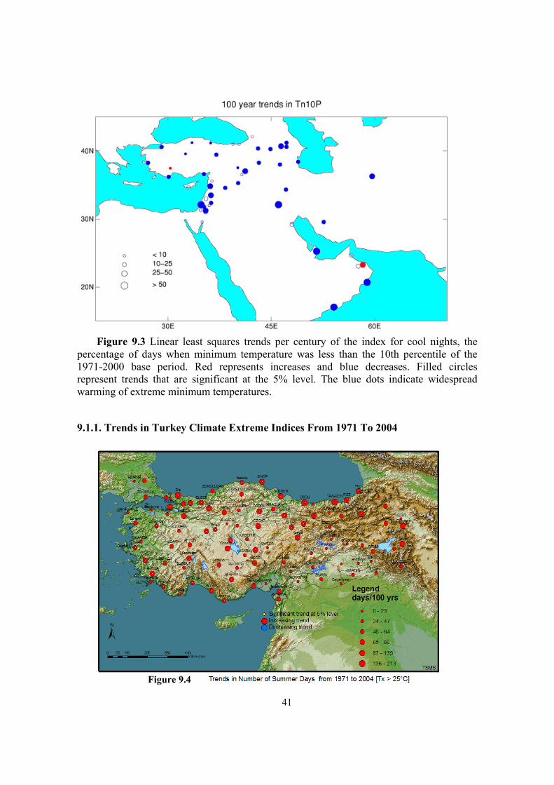
41

Figure 9.3 Linear least squares trends per century of the index for cool nights, the

percentage of days when minimum temperature was less than the 10th percentile of the 1971-2000 base period. Red represents increases and blue decreases. Filled circles represent trends that are significant at the 5% level. The blue dots indicate widespread warming of extreme minimum temperatures.

9.1.1. Trends in Turkey Climate Extreme Indices From 1971 To 2004

Figure 9.4

42

The results show that numbers of summer days and tropical nights have been

increasing all over Turkey while ice days and frost days decreasing. Summer days have increased about 6 days per decade. Most of the trends are statistically significant at the 5% level. Growing season length has increased over Turkey except for coastal regions. This will be having a positive effect on summer agricultural products but some negative affects will be experienced by orchards for example which rely on cold conditions. Maximum of maximum, minimum of maximum, maximum of minimum and minimum of minimum temperatures have increased at most stations. Warm days and warm nights have been increasing all over Turkey while cool days and cool nights have been decreasing. Warm spells have increased while cold spells have decreased. Diurnal temperature range has increased in most inland stations while it has decreased along coastal areas.

Trends in simple daily intensity index have been increasing in most of the stations even

mean annual total precipitation declined in 30 stations located in the Aegean and inland Anatolia. The number of heavy precipitations days have been increasing especially in the Black Sea and Mediterranean regions and usually cause extreme flood events. The maximum one-day and 5 days precipitation have also increased except eastern Marmara and south Anatolia region. Consecutive dry days have decreased especially in Konya, Karapınar, Ceylanpınar and Iğdır which are suffering drought problem but unfortunately there are increasing trends in Marmara, Aegean and the Black Sea Region. Consecutive wet days have increased especially in eastern parts of the Marmara and around Afyon, Burdur, Niğde, Sinop, Sivas, Rize, Kilis and Muş while decreasing in the Aegean and Konya.

In summary, in general there are large coherent patterns of warming across in the

country affecting both maximum and minimum temperatures but there is a much more mixed pattern of change in precipitation (Sensoy, S., et all, 2007).

9.2. Monthly, seasonal and annual climate assessments

Monthly, seasonal and annual climatological analyses have been doing by using real

time data. It is using ArcGIS for interpolation and monitoring purpose. Also it is calculating their differences from normal. Anomaly is the differences from normal and it is determining by using Z standardized normal distribution (Z=(X-Xmean) /STD). If Z < -0.97 it means that this station value is below normal, if Z is between -0.97 to 0.97, near normal, and if Z > 0.97 it means this value over normal. Calculations have been done by using Excel and then it is loaded personal geodatabase in order to produce maps.

43

Figure 9.5 Mean temperature anomaly in July, 2009 According to above map in July 2009 western parts of Turkey and Black sea cost have above normal temperature while remaining area near normal except Sivas, Agri and Adiyaman.

Figure 9.6 Turkey mean temperature anomaly in Spring 2009 Turkey mean temperature (1961-1990) in summer is 23.0°C. Mean temperature in summer 2009 was 23.6°C. In this result, 2009 summer was 0.6°C above normal.

9.2.1. Assessment of 2008 climatic variable

2008 mean temperature was 0.8°C above the 1961-1990 average (13.6°C). Generally coastal area and western part of the country had temperatures above the mean while around Sivas, Erzurum and Kars had below it. Positive temperature anomalies have been occurred since 1994 (except 1997) (Fig. 9.7)

44

Figure 9.7 Spatial and temporal temperature and precipitation anomalies in 2008 in Turkey Important decreases has been occurred in total precipitation in Antalya, Muğla, Mardin and Bitlis while slight increases has been occurred in central Black Sea region, Sivas, Bayburt and Kars in the year 2008. Mean total precipitation was 128mm below the 1961-1990 mean (Fig. 9.7).

Despite the droughts conditions, 42 extreme rainfall and floods events occurred in some places. The other extreme events occurred frequently in Turkey are storm, hail and drought (Fig. 9.8). (Sensoy, 2009).

Figure 9.8 Extreme events occurred in Turkey in 2008

45

9.3. Heating and Cooling Degree-Days Heating degree-day is the unit which useful to indicate how much time cold in the day. Heating Degree Days (HDD): In the given time (day, month, year) it explains intensity

of cold by considering indoor and outdoor temperature. Most of the country are been using different formula to calculate degree-day. In order to make common application European statistic Office (Eurostat) suggested following formula to calculate HDD (Gikas et all., 2006).

HDD = (18 °C - Tm) x d, if Tm ≤ 15 °C (heating threshold) than HDD = 0 Where; Tm = Daily mean temperature, d= N. of days Calculation has been done for daily bases than monthly and annual valu are calculated. Cooling Degree Days (CDD): In the given time (day, month, year) it explains intensity

of warm by considering indoor and outdoor temperature. Most of the country are been using different formula to calculate degree-day. There is no official threshold temperature but construction sector has been accepted 22°C as air conditioning threshold. So:

CDD = (Tm - 22) x d if Tm ≥ 22°C (cooling threshold) than CDD = 0 Where; Tm = Daily mean temperature, d= N. of days To know total heating and cooling degree-days are very important in order to calculate

energy demand for heating and air conditioning of building. If daily mean temperature is above 15°C there is not necessary to heat. Heating cost is directly related with annual HDD. For this purpose firstly 30 years average (normal) HDD shuld be calculated. If the annual total fuel cost devided with mean annual HDD, this is the heating cost for 1 HDD. This indis can be use for future calculation. HDD could be used also to compare intensity of winter season with the other winters. HDD also needed parameter by construction sectors while design of building in order to calculate, insulation, heating and cooling cost.

In this study by using 130 stations value, heating and cooling degree days for 2006

were calculated for each month and compared with 30 years normal. According to results; while heating requirements have been increasing in Marmara, Aegean, central Black Sea, Adana, Hatay, Bingöl, Diyarbakır and Batman; decreasing in eastern part of Turkey because of the above normal temperature. This decreasing is contrasted with increasing temperature. Also as parallel with increasing temperature in 2006, especially in southeastern and central Anatolia, cooling degree days have been increased in all Turkey.

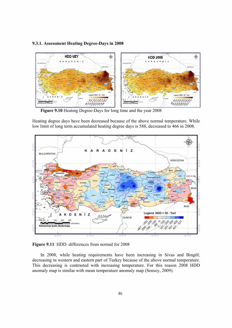
46

9.3.1. Assessment Heating Degree-Days in 2008

Figure 9.10 Heatıng Degree-Days for long time and the year 2008

Heating degree days have been decreased because of the above normal temperature. While low limit of long term accumulated heating degree days is 588, decreased to 466 in 2008.

Figure 9.11 HDD differences from normal for 2008 In 2008, while heating requirements have been increasing in Sivas and Bingöl;

decreasing in western and eastern part of Turkey because of the above normal temperature. This decreasing is contrasted with increasing temperature. For this reason 2008 HDD anomaly map is similar with mean temperature anomaly map (Sensoy, 2009).

47

9.3.2. Assessment of 2008 Cooling Degree-Days

Figure 9.12 Cooling Degree-Days for long time and the year 2008

While low upper limit of long term accumulated cooling degree days is 1243 increased to 1587 in 2008. Cooling degree-days was increased especially southern part of the Turkey in 2008

Figure 9.13 CDD Differences from normal for 2008 As parallel with increasing temperature in 2008, especially in southwestern part, Hopa

and Cizre, cooling degree days have been increased.

48

9.4. Climate Classification

The purpose of classification is to organize a set of data or information about something to effectively communicate it in an informative way. Classification helps synthesize information into smaller units that are more easily understood. When considering the Earth's climate, there is such an enormous amount of information that one has to break it down into areas of commonality to easily understand it. Climatologists have therefore created several ways to organize the wealth of information about Earth's climate to bring order and understanding to it.

9.4.1. Köeppen’s climate classification There are many different regional climates across the world. To make sense of this

variability we devise classification schemes in which important characteristics of a phenomenon are grouped into classes that have things in common. Classification is a process common to all sciences.

The goal of classification is to identify and group together things that have similar

characteristics. Climate classifications describe the world's climates. The problem with classifying climates is that there are few sharp dividing lines between different climates. There are gradual transitions from one climate to another.

A challenge in designing a climate classification scheme is that climates fluctuates and

transition zones often exist between two very different climate regions, making sharp boundaries difficult to establish. One of the simplest climate classification schemes is based on solar illumination. This approach does have sharp boundaries.

Temperature and precipitation are two important climate variables. These two

parameters typically define the type of vegetation that can grow in the region. It is therefore useful to classify climate according to these variables.

The most widely used climate classification schemes are those of Köppen. Vladimir

Köppen developed his classification system from 1918 to 1936. He used vegetation and temperature as a natural indication of the climate of a region. There have been improvements made to the original Köppen scheme, particularly by Trewartha and Horn. The current classification scheme has six main groups, each designated with a letter: Tropical Moist (A), Dry (B), Moist with Mild Winters (C), Moist with Severe Winters (D), Polar (E), and Highland (H). Figure 9.14 organizes these climate groups by their temperature and precipitation characteristics. Climates A, C, D, E, and H are based on temperature while B climates focus on precipitation differences.

Division of the six main categories provides additional classifications. The next

sections provide more detail on the climate in each major group.

49

Tropical Humid Climates (A) The mean monthly temperature of Tropical Humid climates is high, no lower than

65°F (18.3°C) with small annual variations, typically less than 18°F (10°C). Killing frosts are absent in A type climate regions. The diurnal variation in temperature in A climate regions is often larger than the annual variation.

Tropical Wet, dry and monsoon (Af, Aw and Am) While Tropical Humid climates have abundant rainfall (typically more than 100 cm or

39 in per year) they can have different precipitation patterns. A type climate zones are therefore subdivided into three subtypes: tropical wet climates (Af), tropical wet-and-dry climates (Aw), and tropical monsoon (Am). Examples of these climates are Iquitos, Peru (Af), Asunicion Paraguay (Aw), and Manaus, Brazil (Am). Figure 9.14 shows the annual temperature and precipitation patterns of these cities.

The tropical wet climates, Af, have temperature that is distributed fairly uniformly throughout the year. Total precipitation over a year averages between 6.9 -10 inches (17.5 - 25.0 cm). The precipitation amount for each month is at least 2.4 inches (6 cm). Af also has a diurnal precipitation pattern, with most thunderstorms occurring in the afternoon, triggered by solar heating of the surface. Vegetation in Af climates is very lush, such as the tropical rainforests of Brazil and the Congo.

Tropical wet-and-dry climates, Aw, have a dry season. Summers are wet and winters

are dry in Aw climates. This seasonal rainfall is linked to the season migration of the InterTropical Convergence Zone. There is a cool season in Aw climates, which occurs during winter. Analysis of Figure 14.19 shows that Aw often border Af. The vegetation of Aw climates is typically savanna or tropical grasslands with scattered deciduous trees, as in the grasslands of Africa.

Tropical monsoon climates, Am, are monsoon climates that have a short dry season.

Monthly average temperatures of Am climates are uniform throughout the year. These climates tend to occur in regions that have seasonal onshore winds to supply an ample supply of moist air. Orographic lifting also helps to enhance the precipitation of Am regimes.

Dry Climates (B) Dry climate zones (B) are located in regions where evaporation exceeds precipitation.

Rainfall is highly variable in these B climate zones. Most of the land regions of the world are designated as B climate zones! The descending branch of the Hadley cell or a rain shadow caused by mountain barriers causes lack of precipitation in many of the B climate zones.

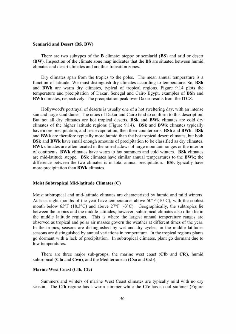
50

Semiarid and Desert (BS, BW) There are two subtypes of the B climate: steppe or semiarid (BS) and arid or desert

(BW). Inspection of the climate zone map indicates that the BS are situated between humid climates and desert climates and are thus transition zones.

Dry climates span from the tropics to the poles. The mean annual temperature is a

function of latitude. We must distinguish dry climates according to temperature. So, BSh and BWh are warm dry climates, typical of tropical regions. Figure 9.14 plots the temperature and precipitation of Dakar, Senegal and Cairo Egypt, examples of BSh and BWh climates, respectively. The precipitation peak over Dakar results from the ITCZ.

Hollywood's portrayal of deserts is usually one of a hot sweltering day, with an intense

sun and large sand dunes. The cities of Dakar and Cairo tend to conform to this description. But not all dry climates are hot tropical deserts. BSk and BWk climates are cold dry climates of the higher latitude regions (Figure 9.14). BSk and BWk climates typically have more precipitation, and less evaporation, then their counterparts, BSh and BWh. BSk and BWk are therefore typically more humid than the hot tropical desert climates, but both BSk and BWk have small enough amounts of precipitation to be classified as dry climates. BWk climates are often located in the rain-shadows of large mountain ranges or the interior of continents. BWk climates have warm to hot summers and cold winters. BSk climates are mid-latitude steppe. BSk climates have similar annual temperatures to the BWk; the difference between the two climates is in total annual precipitation. BSk typically have more precipitation than BWk climates.

Moist Subtropical Mid-latitude Climates (C)

Moist subtropical and mid-latitude climates are characterized by humid and mild winters. At least eight months of the year have temperatures above 50°F (10°C), with the coolest month below 65°F (18.3°C) and above 27°F (-3°C). Geographically, the subtropics lie between the tropics and the middle latitudes; however, subtropical climates also often lie in the middle latitude regions. This is where the largest annual temperature ranges are observed as tropical and polar air masses govern the weather at different times of the year. In the tropics, seasons are distinguished by wet and dry cycles; in the middle latitudes seasons are distinguished by annual variations in temperature. In the tropical regions plants go dormant with a lack of precipitation. In subtropical climates, plant go dormant due to low temperatures.

There are three major sub-groups, the marine west coast (Cfb and Cfc), humid

subtropical (Cfa and Cwa), and the Mediterranean (Csa and Csb).

Marine West Coast (Cfb, Cfc) Summers and winters of marine West Coast climates are typically mild with no dry

season. The Cfb regime has a warm summer while the Cfc has a cool summer (Figure

51

9.14). Cfb and Cfc climates are usually near the coast. The characteristic temperature and precipitation is determined by the advection of air over ocean currents. This moderates the annual range in temperature. When cool water is up wind, the summer high temperatures are primarily moderated, while warmer ocean currents lead to milder winter temperatures. The coldest month of the year has an average temperature above freezing, making snowfall rare. The name of this climate type, marine west coast, suggests that these climates lie along the west coasts of continents. However, these climates are also found along southeastern Australia and southeastern Africa.

Humid sub-tropical (Cfa, Cwa) Humid sub-tropical climates have hot summers (Figure 9.14). These climate regimes

occur in the mid-latitudes regions. Daytime high temperatures typical of this regime are in the 80° to 90°F range. The humid conditions, dewpoints in the 70s, keep the low temperatures in the evening from getting very cold. Winter temperatures are mild. While mean temperatures may be above freezing in winter, it is not uncommon for the temperatures to drop below 32°F (0°C). Precipitation in humid sub-tropical climates is plentiful, 30 to 100 in (75 to 250 cm) per year. Summer precipitation is usually associated with convection and mid-latitude cyclones bring the winter precipitation. Cfa climates are wet all year round while Cwa regions have a brief dry season in the winter. Summer precipitation in both climates is primarily convective.

Mediterranean (Csa, Csb) Mediterranean climates are characterized by little precipitation in the summer (Figure

9.14). This particular climate classification has a peak in precipitation during winter. The lack of precipitation in summer is associated with the presence of a high-pressure system that moves into the region and stays. Summer temperatures range from hot to mild and winter temperatures are mild. When located along a coast, winter temperatures are very mild. Winter temperatures can drop below freezing if far from the modifying influences of a large body of water.

Severe Mid-latitude Climates (D) The severe mid-latitude climates (D) are located in the eastern regions of continents.

So, the temperature range of the D climate regimes is generally greater than C climate types, which tend to be located on the west side of continents. The average temperature of the coldest month of a D type climate regime must be less than 27°F (-3°C). These climate types typically have snow on the ground for extended periods of time. There a two basic D climate types, humid continental and subarctic. These subgroups are further divided into groups based on precipitation and summer temperature. The second letter f indicates that the climate has no dry season, while a second letter of w indicates a dry season in winter.

For D climates, a third letter of a, b or c indications a hot summer, a warm summer, or

a cool summer, respectively. A hot summer climate has a warmest month of about 72F

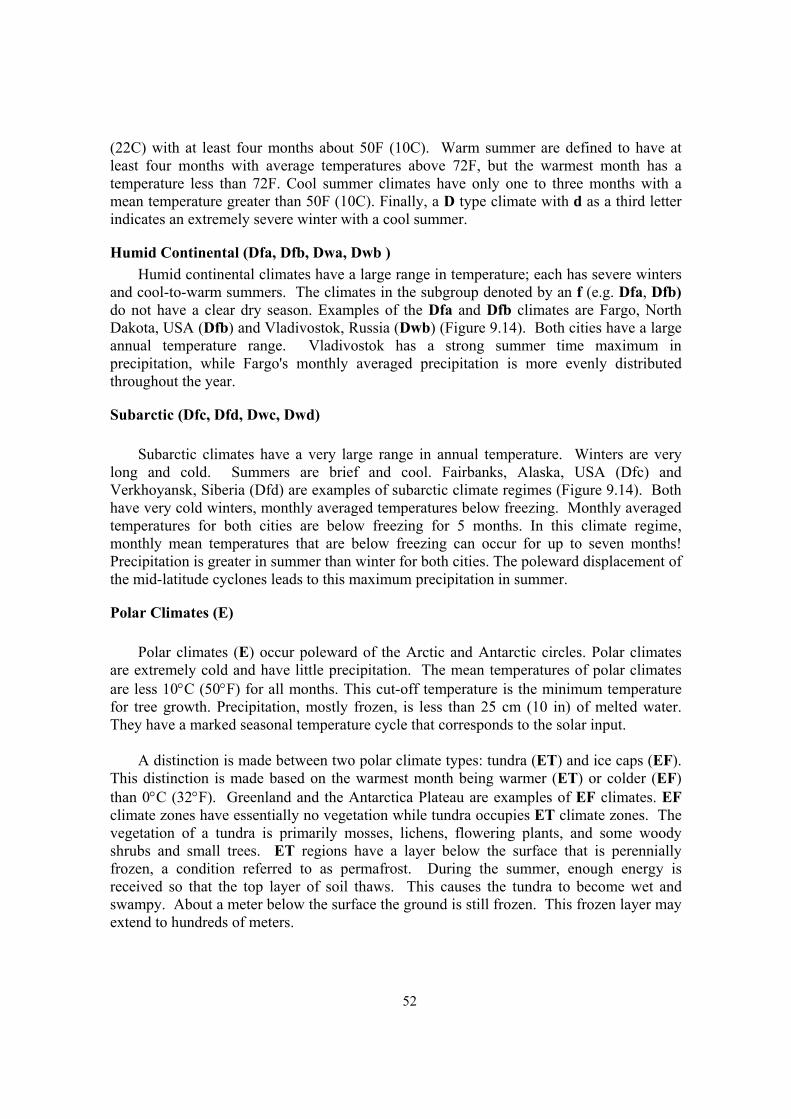
52

(22C) with at least four months about 50F (10C). Warm summer are defined to have at least four months with average temperatures above 72F, but the warmest month has a temperature less than 72F. Cool summer climates have only one to three months with a mean temperature greater than 50F (10C). Finally, a D type climate with d as a third letter indicates an extremely severe winter with a cool summer.

Humid Continental (Dfa, Dfb, Dwa, Dwb ) Humid continental climates have a large range in temperature; each has severe winters

and cool-to-warm summers. The climates in the subgroup denoted by an f (e.g. Dfa, Dfb) do not have a clear dry season. Examples of the Dfa and Dfb climates are Fargo, North Dakota, USA (Dfb) and Vladivostok, Russia (Dwb) (Figure 9.14). Both cities have a large annual temperature range. Vladivostok has a strong summer time maximum in precipitation, while Fargo's monthly averaged precipitation is more evenly distributed throughout the year.

Subarctic (Dfc, Dfd, Dwc, Dwd) Subarctic climates have a very large range in annual temperature. Winters are very

long and cold. Summers are brief and cool. Fairbanks, Alaska, USA (Dfc) and Verkhoyansk, Siberia (Dfd) are examples of subarctic climate regimes (Figure 9.14). Both have very cold winters, monthly averaged temperatures below freezing. Monthly averaged temperatures for both cities are below freezing for 5 months. In this climate regime, monthly mean temperatures that are below freezing can occur for up to seven months! Precipitation is greater in summer than winter for both cities. The poleward displacement of the mid-latitude cyclones leads to this maximum precipitation in summer.

Polar Climates (E) Polar climates (E) occur poleward of the Arctic and Antarctic circles. Polar climates

are extremely cold and have little precipitation. The mean temperatures of polar climates are less 10°C (50°F) for all months. This cut-off temperature is the minimum temperature for tree growth. Precipitation, mostly frozen, is less than 25 cm (10 in) of melted water. They have a marked seasonal temperature cycle that corresponds to the solar input.

A distinction is made between two polar climate types: tundra (ET) and ice caps (EF).

This distinction is made based on the warmest month being warmer (ET) or colder (EF) than 0°C (32°F). Greenland and the Antarctica Plateau are examples of EF climates. EF climate zones have essentially no vegetation while tundra occupies ET climate zones. The vegetation of a tundra is primarily mosses, lichens, flowering plants, and some woody shrubs and small trees. ET regions have a layer below the surface that is perennially frozen, a condition referred to as permafrost. During the summer, enough energy is received so that the top layer of soil thaws. This causes the tundra to become wet and swampy. About a meter below the surface the ground is still frozen. This frozen layer may extend to hundreds of meters.

53

Precipitation in Polar climates is very low, sometimes less than the tropical deserts. However, these regions are not considered deserts because precipitation exceeds evaporation.

Highland Climates (H) The elevation above sea level is an important climate variable. Highland climates (H)

characterize the type of climates associated with high mountainous terrain. These climate zones are complex and driven by changes in latitude, altitude, and exposure. A wide variety of climates are exhibited in H climate zones. As noted in Chapter 3, temperature usually decreases with height in the troposphere. The temperature of a mountain location will strongly depend on the slope angle and aspect, which influences the amount of solar energy received. A common feature of a highland climate is the large diurnal temperature variation. Rapid daytime heating and nighttime cooling results because of the thin dry air. Mountains have a large variation in precipitation. The amount depends on the orientation of the highland, atmospheric moisture and prevailing wind directions. The leeward side is a rain shadow while the windward side can have heavy rainfall.

Figure 9.14 World Climate patterns according to Koeppen (FAO)

9.4.2. Trewartha’s climate classification

The Trewartha climate classification scheme is a modified version of the Köppen system. It attempts to redefine the broad climatic groups in such a way as to be closer to vegetational zoning. - Group A: This the tropical climate group, defined the same as in Köppen's scheme (i.e., all 12 months average 18 °C or above). Climates with no more than two dry months

54

(defined as having less than 60mm average precipitation, same as per Köppen) are classified Ar (instead of Köppen's Af), while others are classified Aw if the dry season is at the time of low sun/short days or As if the dry season is at the time of high sun/long days. There was no specific monsoon climate identifier in the original scheme, but Am was added later, with the same parameters as Köppen's (except that at least three months, rather than one, must have less than 60mm average precipitation). - Group B: BW and BS mean the same as in the Köppen scheme, with the Köppen BWn climate sometimes being designated BM (the M standing for "marine"). However, a different formula is used to quantify the aridity threshold: 10 X (T − 10) + 3P, with T equalling the mean annual temperature in degrees Celsius and P denoting the percentage of total precipitation received in the six high-sun months (April through September in the Northern Hemisphere and October through March in the Southern). If the precipition for a given location is less than the above formula, its climate is said to be that of a desert (BW); if it is equal to or greater than the above formula but less than twice that amount, the climate is classified as steppe (BS); and if the precipitation is more than double the value of the formula the climate is not in Group B. Unlike in Köppen's scheme, no thermal subsets exist within this group in Trewartha's, unless the Universal Thermal Scale (see below) is used. - Group C: In the Trewartha scheme this category encompasses subtropical climates only (8 or more months above 10 °C). Cs and Cw have the same meanings as they do in Köppen's scheme, but the subtropical climate with no distinct dry season is designated Cr instead of Köppen's Cf (and for Cs the average annual precipitation must be less than 890mm [35 inches] in addition to the driest summer month having less than 30mm precipitation and being less than one-third as wet as the wettest winter month). - Group D: This group represents temperate climates (4 to 7 months above 10 °C). Maritime temperate climates (most of Köppen's Cfb and Cwb climates, though some of these would fit into Trewartha's Cr and Cw respectively) are denoted DO in the Trewartha classification (although some places near the east coasts of both North America and Asia actually qualify as DO climates in Trewartha's scheme when they fit into Cfa/Cwa rather than Cfb/Cwb in Köppen's), while continental climates are represented as DCa (Köppen Dfa, Dwa, Dsa) and DCb (Köppen Dfb, Dwb, Dsb). For the continental climates, sometimes the third letter (a or b) is omitted and DC is simply used instead, and occasionally a precipitational seasonality letter is added to both the maritime and continental climates (r, w, or s, as applicable). The dividing point between the maritime and continental climates is 0 °C in the coldest month, rather than the Köppen value of −3 °C (as noted in the section on the Köppen scheme, however, some climatologists — particularly in the United States — now observe 0 °C in the coldest month as the equator ward limit of the continental climates in that scheme as well). - Group E: This represents subarctic climates, defined the same as in Köppen's scheme (1 to 3 months with average temperatures of 10 °C or above; Köppen Cfc, Dfc, Dwc, Dsc, Dfd, Dwd). In the original scheme, this group was not further divided; later, the designations EO and EC were created, with EO (maritime subarctic) signifying that the coldest month averages above −10 °C, while EC (continental subartctic or "boreal") means

55

that at least one month has an average temperature of −10 °C or below. As in Group D, a third letter can be added to indicate seasonality of precipitation. There is no separate counterpart to the Köppen Dfd/Dwd climate in Trewartha's scheme. - Group F: This is the polar climate group, split into FT (Köppen ET) and FI (Köppen EF). - Group H: Highland climates, in which altitude plays a role in determining climate classification. Specifically, this would apply if correcting the average temperature of each month to a sea-level value using the formula of adding 5.6°C for each 1,000 meters of elevation would result in the climate fitting into a different thermal group than that into which the actual monthly temperatures place it. Sometimes G is used instead of H if the above is true and the altitude is 500 meters or higher but lower than 2,500 meters; but the G or H is placed in front of the applicable thermal letter rather than replacing it — and the second letter used reflects the corrected monthly temperatures, not the actual monthly temperatures. - Universal Thermal Scale: An option exists to include information on both the warmest and coldest months for every climate by adding a third and fourth letter, respectively. The letters used conform to the following scale: i — severely hot: Mean monthly temperature 35 °C or higher h — very hot: 28 to 34.9°C a — hot: 23 to 27.9°C b — warm: 18 to 22.9°C l — mild: 10 to 17.9°C k — cool: 0.1 to 9.9°C o — cold: −9.9 to 0 °C c — very cold: −24.9 to −10 °C d — severely cold: −39.9 to −25 °C e — excessively cold: −40 °C or below. 9.4.3. Aydeniz’s Climate Classification

AYDENİZ METHOD: YxNn Formula: Nks= x Np (yıllık) SxGS+15 1 Drought coefficient = Kks = dir. (DMI, 1988) Nks Where:: Y : Precipitation Nn : RH S : Temperature G : Sunshine

56

Np : percentage of humidity period (N.of Nks > 0.40/12). In monthly calculation Np=12 Table 3 Aydeniz index and climate types

Kks Characteristic Nks >2.50 Desert <0.4 1.50 – 2.50 Very dry 0.40 – 0.67 1.00 – 1.50 Dry 0.67 – 1.00 0.75 – 1.00 Semi dry 1.00 - 1.33 0.50 – 0.75 Semi-humide 1.33 – 2.00 0.25 – 0.50 Humide 2.00 – 4.00 <0.25 Wet >4.00

Figure 9.15 Climate Classifications of Turkey By Aydeniz Method (Şensoy S, 2006) The driest regions are the Karaman, Malatya, Iğdır and Şanlıurfa, where annual rainfall frequently is less than 300 millimeters. The wettest regions are the Black Sea coastal regions where annual rainfall can reach 2,200 millimeters annually. 9.4.4. De Martonne’s Climate Classification

De Martonne Climate Classification considers precipitation and temperature with

the other parameters. Beside the annual precipitation and temperature, January and July precipitation and temperature have been considered in calculation. Annual precipitation amount give the possibility to separate rainy and dry climate. To determine dry period it’s

57

important evaporation beside the precipitation. (DMİ,1972). De Martonne annual dry indices formula which generated with Gottmann are as follows:

Ia = (P / (T + 10) + (12 * p /(t + 10)))/2 Table 4. De Martonne index and climate types Where;

10 = Constant P = Precipitation T = Mean temperature(°C). p = July precip. (mm); t = July Temp.(°C)

Calculation for Konya; Ia = (315/(11.5+10) + (12*3.7/(22.9+10)))/2 = 8 According to result Konya is step climate

Figure 9.16 Climate Classifications of Turkey by De Martonne Method (Sensoy, S., 2006)

Climate types dry index Desert 0 – 5 Step 5 – 10 Step-

moist 10 - 20

Semi humid 20 - 28

Humid 28 - 35 Very

humid 35 - 55

Wet > 55

Arctic < 0 (T < -5 C)

58

9.4.5. Erinc’s Climate Classification

Indice generated by precipitation/mean temperature give the wrong result (more humid than reality) in terrestrial area. For this reason Erinç take mean maximum temperature instead of mean temperature for his calculation. In his formula some months dont be considered where mean maximum temperature below 0°C due to there is no evaporation there.

Precipitation effectivness indice omTP

=Im where,

P = annual total precip. (mm), Tom = annual mean max. temp. (Erinç, S., 1984) Erinç defined 6 climate type according to index result: Table 5. Erinç index and climate types Climate types İndex (Im) Plant cover Very dry <8 Desert Dry 8-15 Desert-step Semi dry 15-23 Step Semi humid 23-40 Dry forest Humid 40-55 Moist forest Very humid >55 V. Moist forest

Figure 9.17 Climate Classifications of Turkey by Erinc Method (Sensoy, S., 2006)

59

9.4.6. Thornthwaite’s Climate Classification

Thornthwaite climate classification depends on precipitation - evaporation and temperature - evaporation relations. According to Thornthwaite, if precipitation more than evaporation there soil is wet. On the other hand, if precipitation is less than evaporation there is water deficit there. Soil couldn’t be given enough water to plant. So this area is dry. Rainfall effectiveness indice Table 6. Thornthwaite index and climate types

ETPdS 60100Im −

= where;

S = annual water surplus, d = annual water deficit ETP = annual evapotranspiration

Calculation for Şanlıurfa:

261030

)8.76160()193100(Im −=−

=xx

Şanlıurfa 1st. letter is D

Figure 9.18 Climate Classifications of Turkey by Thornthwaite Method (Sensoy, S., 2006)

Im Letter Climate types >100 A Very humid 100-80 B4 Humid 80-60 B3 Humid 60-40 B2 Humid 40-20 B1 Humid 20-0 C2 Semi humid 0-(-20) C1 S. dry-less humid -20-(-40) D Semi dry -40-(-60) E Dry

60

9.4.7. Climate diagrams Climographs are plots of climatic data. Climographs usually consist of two climatic elements plotted through an annual cycle.

Figure 9.19 Climate diagram of some cities in Turkey Antalya graph represent rainy winter, hot and dry summer (Mediterranean climate) while Hopa graph represent rainy mild climate in every month (Black Sea climate)

Figure 9.20 Climogram of some cities in Turkey If obtained shape is long as Antalya’s it means that there is big difference between seasons. If shape is spherical like Hopa’s it means that there is no big difference between seasons in terms of temperature and precipitation.

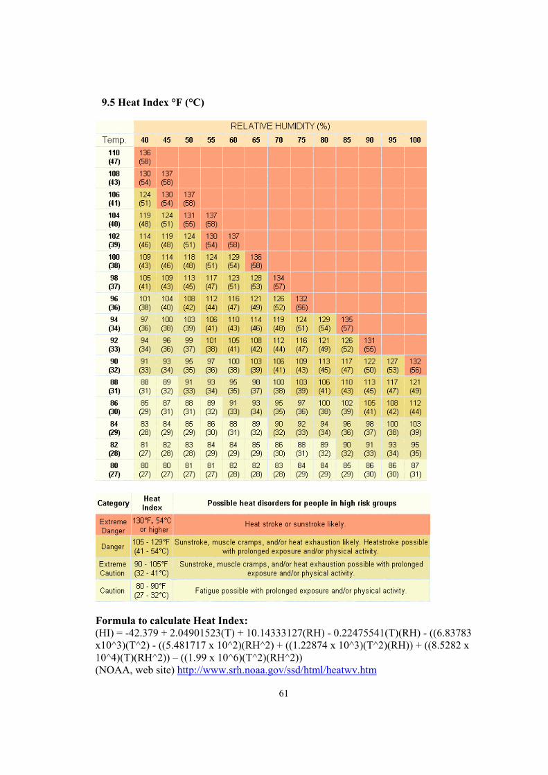
61

9.5 Heat Index °F (°C)

Formula to calculate Heat Index: (HI) = -42.379 + 2.04901523(T) + 10.14333127(RH) - 0.22475541(T)(RH) - ((6.83783 x10^3)(T^2) - ((5.481717 x 10^2)(RH^2) + ((1.22874 x 10^3)(T^2)(RH)) + ((8.5282 x 10^4)(T)(RH^2)) – ((1.99 x 10^6)(T^2)(RH^2)) (NOAA, web site) http://www.srh.noaa.gov/ssd/html/heatwv.htm

62

9.6. Climate Atlas

Long term corrected, quality controlled, homogenized climate data are required for climate atlas studies. Last official climatic period is 1961-2000 by WMO but most of the countries changed their climatic period as 1971-2000.

To produce climate Atlas of Turkey, we are using 1971-2000 climatic period.

Geographic variables are measured at certain points, and prediction map for the entire area is been obtained by some spatial interpolation methods. Spatial distribution of geographic data can be obtained only from this data and also prediction map can be obtained by using secondary variables which have spatial relationship with the measured values (Bostan, P.A., et al, 2007)

Geographically Weighted Regression (GWR) and Co-kriging methods can be applied in the modelling of parameters. GWR is the multi-faceted approach to the analysis of spatial data. GWR opens a window through the data set to calculate local r2 (Laffan, 1999). Co-kriging is an extension of ordinary kriging method which takes into account the spatial cross-validation between two or more data.

Figure 9.21 Solar energy atlas of Turkey There are 522 maps related to 34 climate parameters, 130 maps related to counted

days, and 27 climate indices maps totally 679 maps have been created (Figure 40.)

63

Summary Climate varies from location to location, and with time. Climatology and

paleoclimatology attempt to organize the complex and varied climates of the world through classification systems. It is quite amazing that, through scientific evidence, we have a general idea of Earth's climate since the beginning of Earth's history.

Evidence indicates that during most of the Earth's past 500 million years the Earth was

a more genial climate than today. This mild climate was interrupted by occasional ice ages. Climatic zones where present, but were less distinct than they are today. Several theories have been put forth to explain the change between glacial and interglacial periods. Continental drift is an important part of understanding very long-term climate changes. Additional theories, variations in the Earth's orbit, changes in the output of the sun, and changes in atmospheric composition.

Over the past 20 years, global temperatures have steadily increased. Some of this

increase may be a result of human activity. Today, the Köppen based climate classification is the most widely used scheme for

mapping climates of the world. The Köppen scheme is just one method of classifying climate. Different schemes could be developed based on the purpose of the user. For example, the Köppen scheme would not be very useful for wind energy applications. A scheme could therefore be devised that is based on wind speed and direction. For hydrological applications we might want a scheme based on the type of precipitation, not just monthly mean precipitation. Thornthwaite developed a classification scheme based on the water budget of a region.

To know total heating and cooling degree-days are very important in order to calculate energy demand for heating and air conditioning of building. If daily mean temperature is above 15°C there is not necessary to heat. Heating cost is directly related with annual HDD. For this purpose firstly 30 years average (normal) HDD shuld be calculated. If the annual total fuel cost devided with mean annual HDD, this is the heating cost for 1 HDD. This indice can be use for future calculation. HDD could be used also to compare intensity of winter season with the other winters. HDD also needed parameter by construction sectors while design of building in order to calculate, insulation, heating and cooling cost.

Under future climate change demand for heating decreases and demand for cooling

increases (Santos et al., 2002) Estimated up to 10% decrease in energy heating requirements and up to 28% increase in cooling requirements in 2030 for the southeast Mediterranean region. Summer space cooling needs for air conditioning will particularly affect electricity demand (Valor et all., 2001). GIS software usage in climatological applications makes increase in product quality and monitoring capability. So the end-users could be understand their lived temperatures were below or above normal, or understand why their energy demand increased.

64

If we know the status of the climate today and the differences between this and the recent past, we can begin to plan for the future. (Obasi G.O.P, 2001)

65

References 1- http://en.wikipedia.org/wiki/Atmospheric_sciences 2- http://en.wikipedia.org/wiki/Climate 3- M. Allaby, The Facts on Weather and Climate Handbook, 2002, New York 4- S.Sensoy, Climate Application, 2007, Ankara 5- http://en.wikipedia.org/wiki/Climatology 6- WMO Guide to Climatological Practices Drift Third Edition,2007, Geneva 7- Dr. J. Hann, Hand book of Climatology, 1903, London 8- http://www.tpub-

products.com/archive/?../../subscribers/./Meteorology/Naval_Aerographer/main.htm 9- G.V.Jones, http://www.sou.edu/Geography/JONES/GEOG482/lectures/introduction.pdf

10- http://www.climatescience.gov/infosheets/factsheet2/EarthSysCartoon.jpg 11- Bostan P.A., Akyürek Z., 2007, İkincil Veriler Kullanılarak Türkiye Ortalama Yıllık

Yağış Değerlerinin Mekansal Dağılımının Modellenmesi, TMMOB Harita ve Kadastro Mühendisleri Odası, Ulusal Coğrafi Bilgi Sistemleri Kongresi, 30 Ekim –02 Kasım 2007, KTÜ, Trabzon

12- DMİ., 1972., Türkiye İklim Tasnifi (De Martonne Metoduna Göre). Ankara 13- D.M.İ., 1988., Aydeniz Metodu ile Türkiye’nin Kuraklık Değerlendirmesi. Ankara 14- Erinç, S., 1984, Klimatoloji ve Metotları, İ.T.Ü. Deniz Bilimleri ve Coğrafya Enstitüsü,

İstanbul 15- FAO, Food And Agriculture Organization, www.fao.org 16- Gikas, A., R. Keenan, 2006: Profil climatique Degrés jours de chauffage, Statistique en

bref. Environnement et énergie 5/2006 ISSN 1562-3084, Communautés européennes http://epp.eurostat.ec.europa.eu/cache/ITY_OFFPUB/KS-NQ-06-005/FR/KS-NQ-06-005-FR.PDF

17- IPCC, TAR, 2001: Third Assessment Report 18- Kuniholm, I. P. et all, Dendrochronological Dating in Anatolia: The Second

Millennium BC NOAA, NCDC Paleoclimatology web site, http://www.ncdc.noaa.gov/paleo/paleo.html, http://www.srh.noaa.gov/elp/wxcalc/heatindex.html

19- Obasi, G.O.P, 2001 WMO-No 920, WMO Statement On The Status Of The Global Climate in 2001. Geneva, Switzerland

20- Santos, F.D., K. Forbes, and R. Moita (eds.), 2002: Climate Change in Portugal: Scenarios, Impact and Adaptation Measures. SAIM Project report, Gradiva, Lisbon, Portugal, pp456 [Europe; Climate Impacts]

21- Sensoy S, 2006 Climate of Turkey. TSMS web site; http://www.dmi.gov.tr/files/en-US/climateofturkey.pdf

22- Sensoy, S., T. C. Peterson, L. V. Alexander, X. Zhang, 2007: Enhancing Middle East Climate Change Monitoring and Indexes DOI:10.1175/BAMS-88-8-1249 http://ams.allenpress.com/archive/1520-0477/88/8/pdf/i1520-0477-88-8-1249.pdf

23- Sensoy, S., M. Demircan, İ. Alan, 2007: Trends In Turkey Climate Extreme Indices From 1971 to 2004, presented in IUGG Conference Perugia, Italy

24- Sensoy, S., Ulupınar, Y., 2008, Türkiye iklim sınıflandırmaları, D.M.İ. web sitesi, Url: http://www.dmi.gov.tr/2006/iklim/files/iklim_siniflandirmalari.pdf

66

25- Sensoy, S., 2009: Regional Climate, (4) Southwest Asia, (iiii) Turkey [in “State of The Climate in 2008”]. Bull. Amer. Meteor. Soc., 90(8), S163

26- Valor, E., V. Meneu and V. Caselles, 2001: Daily air temperature and electricity load in Spain.

27- J. Appl. Meteor., 40, 1413-1421. [Europe; Energy demand] 28- Zhang, X., et al., 2005, Trends in Middle East climate extreme indices from

1950 to 2003, J.Geophys. Res., 110, D22104, doi: 10.1029/2005JD006181. www.agu.org/pubs/crossref/2005/2005JD006181.shtml