WMO: Guide to Climatological Practices
117
2011 edition Guide to Climatological Practices WMO-No. 100
-
Upload
truongxuyen -
Category
Documents
-
view
250 -
download
6
Transcript of WMO: Guide to Climatological Practices

2011 edition
www.wmo.int
Guide to Climatological Practices
WMO-No. 100
GU
IDE
TO
CLI
MA
TO
LOG
ICA
L P
RA
CT
ICE
SW
MO
-No
. 100
P-C
LW_1
0126
4

Guide to Climatological Practices
WMO-No. 100
2011

© 2011, World Meteorological Organization, Geneva
ISBN 978-92-63-10100-6
Note
The designations employed and the presentation of material in this publication do not imply the expression of any opinion whatsoever on the part of the Secretariat of the World Meteorological Organization concerning the legal status of any country, territory, city or area, or of its authorities, or concerning the delimitation of its frontiers or boundaries.
Page
PREFACE . . . . . . . . . . . . . . . . . . . . . . . . . . . . . . . . . . . . . . . . . . . . . . . . . . . . . . . . . . . . . . . . . . . . . .. vii
CHAPTER.1 ..INTRODUCTION. . . . . . . . . . . . . . . . . . . . . . . . . . . . . . . . . . . . . . . . . . . . . . . . . . . . . .. . 1–1
1.1 Purpose and content of the Guide . . . . . . . . . . . . . . . . . . . . . . . . . . . . . . . . . . . . . . . . . . . . 1–11.2 Climatology . . . . . . . . . . . . . . . . . . . . . . . . . . . . . . . . . . . . . . . . . . . . . . . . . . . . . . . . . . . . . 1–1
1.2.1 History . . . . . . . . . . . . . . . . . . . . . . . . . . . . . . . . . . . . . . . . . . . . . . . . . . . . . . . . . 1–11.2.2 The climate system . . . . . . . . . . . . . . . . . . . . . . . . . . . . . . . . . . . . . . . . . . . . . . . . 1–21.2.3 Uses of climatological information and research . . . . . . . . . . . . . . . . . . . . . . . . . . 1–5
1.3 International climate programmes . . . . . . . . . . . . . . . . . . . . . . . . . . . . . . . . . . . . . . . . . . . . 1–61.4 Global and regional climate activities . . . . . . . . . . . . . . . . . . . . . . . . . . . . . . . . . . . . . . . . . . 1–61.5 National climate activities . . . . . . . . . . . . . . . . . . . . . . . . . . . . . . . . . . . . . . . . . . . . . . . . . . . 1–71.6 References . . . . . . . . . . . . . . . . . . . . . . . . . . . . . . . . . . . . . . . . . . . . . . . . . . . . . . . . . . . . . . 1–9
1.6.1 WMO publications . . . . . . . . . . . . . . . . . . . . . . . . . . . . . . . . . . . . . . . . . . . . . . . . 1–91.6.2 Additional reading . . . . . . . . . . . . . . . . . . . . . . . . . . . . . . . . . . . . . . . . . . . . . . . . 1–9
CHAPTER.2 ..CLIMATE.OBSERVATIONS,.STATIONS.AND.NETWORKS. . . . . . . . . . . . . . . . . . . . . . .. . 2–1
2.1 Introduction . . . . . . . . . . . . . . . . . . . . . . . . . . . . . . . . . . . . . . . . . . . . . . . . . . . . . . . . . . . . . 2–12.2 Climatic elements . . . . . . . . . . . . . . . . . . . . . . . . . . . . . . . . . . . . . . . . . . . . . . . . . . . . . . . . . 2–1
2.2.1 Surface and subsurface elements . . . . . . . . . . . . . . . . . . . . . . . . . . . . . . . . . . . . . . 2–22.2.2 Upper-air elements . . . . . . . . . . . . . . . . . . . . . . . . . . . . . . . . . . . . . . . . . . . . . . . . 2–32.2.3 Elements measured by remote-sensing . . . . . . . . . . . . . . . . . . . . . . . . . . . . . . . . . 2–5
2.3 Instrumentation . . . . . . . . . . . . . . . . . . . . . . . . . . . . . . . . . . . . . . . . . . . . . . . . . . . . . . . . . . 2–52.3.1 Basic surface equipment . . . . . . . . . . . . . . . . . . . . . . . . . . . . . . . . . . . . . . . . . . . . 2–62.3.2 Upper-air instruments . . . . . . . . . . . . . . . . . . . . . . . . . . . . . . . . . . . . . . . . . . . . . . 2–72.3.3 Surface-based remote-sensing . . . . . . . . . . . . . . . . . . . . . . . . . . . . . . . . . . . . . . . . 2–72.3.4 Aircraft-based and space-based remote-sensing . . . . . . . . . . . . . . . . . . . . . . . . . . 2–82.3.5 Calibration of instruments . . . . . . . . . . . . . . . . . . . . . . . . . . . . . . . . . . . . . . . . . . . 2–10
2.4 The siting of climatological stations . . . . . . . . . . . . . . . . . . . . . . . . . . . . . . . . . . . . . . . . . . . 2–102.5 The design of climatological networks . . . . . . . . . . . . . . . . . . . . . . . . . . . . . . . . . . . . . . . . . 2–122.6 Station and network operations . . . . . . . . . . . . . . . . . . . . . . . . . . . . . . . . . . . . . . . . . . . . . . 2–13
2.6.1 Times of observations . . . . . . . . . . . . . . . . . . . . . . . . . . . . . . . . . . . . . . . . . . . . . . 2–132.6.2 Logging and reporting of observations . . . . . . . . . . . . . . . . . . . . . . . . . . . . . . . . . 2–132.6.3 On-site quality control . . . . . . . . . . . . . . . . . . . . . . . . . . . . . . . . . . . . . . . . . . . . . 2–142.6.4 Overall responsibilities of observers . . . . . . . . . . . . . . . . . . . . . . . . . . . . . . . . . . . . 2–142.6.5 Observer training . . . . . . . . . . . . . . . . . . . . . . . . . . . . . . . . . . . . . . . . . . . . . . . . . 2–142.6.6 Station inspections . . . . . . . . . . . . . . . . . . . . . . . . . . . . . . . . . . . . . . . . . . . . . . . . 2–152.6.7 Preserving data homogeneity . . . . . . . . . . . . . . . . . . . . . . . . . . . . . . . . . . . . . . . . 2–162.6.8 Report monitoring at collection centres . . . . . . . . . . . . . . . . . . . . . . . . . . . . . . . . . 2–162.6.9 Station documentation and metadata . . . . . . . . . . . . . . . . . . . . . . . . . . . . . . . . . . 2–16
2.7 References and additional reading . . . . . . . . . . . . . . . . . . . . . . . . . . . . . . . . . . . . . . . . . . . . 2–172.7.1 WMO publications . . . . . . . . . . . . . . . . . . . . . . . . . . . . . . . . . . . . . . . . . . . . . . . . 2–172.7.2 Additional reading . . . . . . . . . . . . . . . . . . . . . . . . . . . . . . . . . . . . . . . . . . . . . . . . 2–18
CHAPTER.3 ..CLIMATE.DATA.MANAGEMENT. . . . . . . . . . . . . . . . . . . . . . . . . . . . . . . . . . . . . . . . . .. . 3–1
3.1 Introduction . . . . . . . . . . . . . . . . . . . . . . . . . . . . . . . . . . . . . . . . . . . . . . . . . . . . . . . . . . . . . 3–13.2 The importance and purpose of managing data . . . . . . . . . . . . . . . . . . . . . . . . . . . . . . . . . . 3–23.3 Climate data management . . . . . . . . . . . . . . . . . . . . . . . . . . . . . . . . . . . . . . . . . . . . . . . . . . 3–2
3.3.1 CDMS design . . . . . . . . . . . . . . . . . . . . . . . . . . . . . . . . . . . . . . . . . . . . . . . . . . . . 3–33.3.2 CDMS data acquisition . . . . . . . . . . . . . . . . . . . . . . . . . . . . . . . . . . . . . . . . . . . . . 3–3
CONTENTS
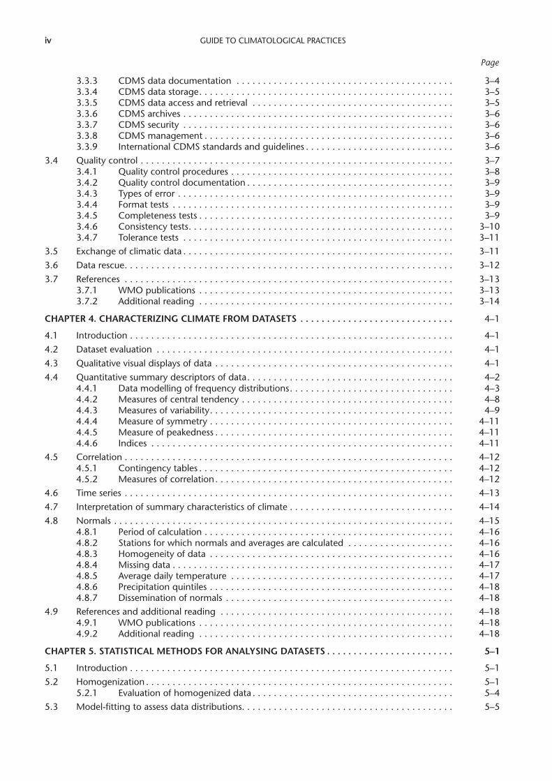
GUIDE TO CLIMATOLOGICAL PRACTICES iv
Page
3.3.3 CDMS data documentation . . . . . . . . . . . . . . . . . . . . . . . . . . . . . . . . . . . . . . . . . 3–43.3.4 CDMS data storage . . . . . . . . . . . . . . . . . . . . . . . . . . . . . . . . . . . . . . . . . . . . . . . . 3–53.3.5 CDMS data access and retrieval . . . . . . . . . . . . . . . . . . . . . . . . . . . . . . . . . . . . . . 3–53.3.6 CDMS archives . . . . . . . . . . . . . . . . . . . . . . . . . . . . . . . . . . . . . . . . . . . . . . . . . . . 3–63.3.7 CDMS security . . . . . . . . . . . . . . . . . . . . . . . . . . . . . . . . . . . . . . . . . . . . . . . . . . . 3–63.3.8 CDMS management . . . . . . . . . . . . . . . . . . . . . . . . . . . . . . . . . . . . . . . . . . . . . . . 3–63.3.9 International CDMS standards and guidelines . . . . . . . . . . . . . . . . . . . . . . . . . . . . 3–6
3.4 Quality control . . . . . . . . . . . . . . . . . . . . . . . . . . . . . . . . . . . . . . . . . . . . . . . . . . . . . . . . . . . 3–73.4.1 Quality control procedures . . . . . . . . . . . . . . . . . . . . . . . . . . . . . . . . . . . . . . . . . . 3–83.4.2 Quality control documentation . . . . . . . . . . . . . . . . . . . . . . . . . . . . . . . . . . . . . . . 3–93.4.3 Types of error . . . . . . . . . . . . . . . . . . . . . . . . . . . . . . . . . . . . . . . . . . . . . . . . . . . . 3–93.4.4 Format tests . . . . . . . . . . . . . . . . . . . . . . . . . . . . . . . . . . . . . . . . . . . . . . . . . . . . . 3–93.4.5 Completeness tests . . . . . . . . . . . . . . . . . . . . . . . . . . . . . . . . . . . . . . . . . . . . . . . . 3–93.4.6 Consistency tests . . . . . . . . . . . . . . . . . . . . . . . . . . . . . . . . . . . . . . . . . . . . . . . . . . 3–103.4.7 Tolerance tests . . . . . . . . . . . . . . . . . . . . . . . . . . . . . . . . . . . . . . . . . . . . . . . . . . . 3–11
3.5 Exchange of climatic data . . . . . . . . . . . . . . . . . . . . . . . . . . . . . . . . . . . . . . . . . . . . . . . . . . . 3–113.6 Data rescue . . . . . . . . . . . . . . . . . . . . . . . . . . . . . . . . . . . . . . . . . . . . . . . . . . . . . . . . . . . . . . 3–123.7 References . . . . . . . . . . . . . . . . . . . . . . . . . . . . . . . . . . . . . . . . . . . . . . . . . . . . . . . . . . . . . . 3–13
3.7.1 WMO publications . . . . . . . . . . . . . . . . . . . . . . . . . . . . . . . . . . . . . . . . . . . . . . . . 3–133.7.2 Additional reading . . . . . . . . . . . . . . . . . . . . . . . . . . . . . . . . . . . . . . . . . . . . . . . . 3–14
CHAPTER.4 ..CHARACTERIZING.CLIMATE.FROM.DATASETS. . . . . . . . . . . . . . . . . . . . . . . . . . . . . .. 4–1
4.1 Introduction . . . . . . . . . . . . . . . . . . . . . . . . . . . . . . . . . . . . . . . . . . . . . . . . . . . . . . . . . . . . . 4–14.2 Dataset evaluation . . . . . . . . . . . . . . . . . . . . . . . . . . . . . . . . . . . . . . . . . . . . . . . . . . . . . . . . 4–14.3 Qualitative visual displays of data . . . . . . . . . . . . . . . . . . . . . . . . . . . . . . . . . . . . . . . . . . . . . 4–14.4 Quantitative summary descriptors of data . . . . . . . . . . . . . . . . . . . . . . . . . . . . . . . . . . . . . . . 4–2
4.4.1 Data modelling of frequency distributions . . . . . . . . . . . . . . . . . . . . . . . . . . . . . . . 4–34.4.2 Measures of central tendency . . . . . . . . . . . . . . . . . . . . . . . . . . . . . . . . . . . . . . . . 4–84.4.3 Measures of variability . . . . . . . . . . . . . . . . . . . . . . . . . . . . . . . . . . . . . . . . . . . . . . 4–94.4.4 Measure of symmetry . . . . . . . . . . . . . . . . . . . . . . . . . . . . . . . . . . . . . . . . . . . . . . 4–114.4.5 Measure of peakedness . . . . . . . . . . . . . . . . . . . . . . . . . . . . . . . . . . . . . . . . . . . . . 4–114.4.6 Indices . . . . . . . . . . . . . . . . . . . . . . . . . . . . . . . . . . . . . . . . . . . . . . . . . . . . . . . . . 4–11
4.5 Correlation . . . . . . . . . . . . . . . . . . . . . . . . . . . . . . . . . . . . . . . . . . . . . . . . . . . . . . . . . . . . . . 4–124.5.1 Contingency tables . . . . . . . . . . . . . . . . . . . . . . . . . . . . . . . . . . . . . . . . . . . . . . . . 4–124.5.2 Measures of correlation . . . . . . . . . . . . . . . . . . . . . . . . . . . . . . . . . . . . . . . . . . . . . 4–12
4.6 Time series . . . . . . . . . . . . . . . . . . . . . . . . . . . . . . . . . . . . . . . . . . . . . . . . . . . . . . . . . . . . . . 4–134.7 Interpretation of summary characteristics of climate . . . . . . . . . . . . . . . . . . . . . . . . . . . . . . . 4–144.8 Normals . . . . . . . . . . . . . . . . . . . . . . . . . . . . . . . . . . . . . . . . . . . . . . . . . . . . . . . . . . . . . . . . 4–15
4.8.1 Period of calculation . . . . . . . . . . . . . . . . . . . . . . . . . . . . . . . . . . . . . . . . . . . . . . . 4–164.8.2 Stations for which normals and averages are calculated . . . . . . . . . . . . . . . . . . . . 4–164.8.3 Homogeneity of data . . . . . . . . . . . . . . . . . . . . . . . . . . . . . . . . . . . . . . . . . . . . . . 4–164.8.4 Missing data . . . . . . . . . . . . . . . . . . . . . . . . . . . . . . . . . . . . . . . . . . . . . . . . . . . . . 4–174.8.5 Average daily temperature . . . . . . . . . . . . . . . . . . . . . . . . . . . . . . . . . . . . . . . . . . 4–174.8.6 Precipitation quintiles . . . . . . . . . . . . . . . . . . . . . . . . . . . . . . . . . . . . . . . . . . . . . . 4–184.8.7 Dissemination of normals . . . . . . . . . . . . . . . . . . . . . . . . . . . . . . . . . . . . . . . . . . . 4–18
4.9 References and additional reading . . . . . . . . . . . . . . . . . . . . . . . . . . . . . . . . . . . . . . . . . . . . 4–184.9.1 WMO publications . . . . . . . . . . . . . . . . . . . . . . . . . . . . . . . . . . . . . . . . . . . . . . . . 4–184.9.2 Additional reading . . . . . . . . . . . . . . . . . . . . . . . . . . . . . . . . . . . . . . . . . . . . . . . . 4–18
CHAPTER.5 ..STATISTICAL.METHODS.FOR.ANALYSING.DATASETS. . . . . . . . . . . . . . . . . . . . . . . . .. . 5–1
5.1 Introduction . . . . . . . . . . . . . . . . . . . . . . . . . . . . . . . . . . . . . . . . . . . . . . . . . . . . . . . . . . . . . 5–15.2 Homogenization . . . . . . . . . . . . . . . . . . . . . . . . . . . . . . . . . . . . . . . . . . . . . . . . . . . . . . . . . . 5–1
5.2.1 Evaluation of homogenized data . . . . . . . . . . . . . . . . . . . . . . . . . . . . . . . . . . . . . . 5–45.3 Model-fitting to assess data distributions. . . . . . . . . . . . . . . . . . . . . . . . . . . . . . . . . . . . . . . . 5–5
iv
CONTENTS v
Page
5.4 Data transformation . . . . . . . . . . . . . . . . . . . . . . . . . . . . . . . . . . . . . . . . . . . . . . . . . . . . . . . 5–65.5 Time series analysis . . . . . . . . . . . . . . . . . . . . . . . . . . . . . . . . . . . . . . . . . . . . . . . . . . . . . . . . 5–65.6 Multivariate analysis . . . . . . . . . . . . . . . . . . . . . . . . . . . . . . . . . . . . . . . . . . . . . . . . . . . . . . . 5–75.7 Comparative analysis . . . . . . . . . . . . . . . . . . . . . . . . . . . . . . . . . . . . . . . . . . . . . . . . . . . . . . 5–85.8 Smoothing . . . . . . . . . . . . . . . . . . . . . . . . . . . . . . . . . . . . . . . . . . . . . . . . . . . . . . . . . . . . . . 5–95.9 Estimating data . . . . . . . . . . . . . . . . . . . . . . . . . . . . . . . . . . . . . . . . . . . . . . . . . . . . . . . . . . . 5–10
5.9.1 Mathematical estimation methods . . . . . . . . . . . . . . . . . . . . . . . . . . . . . . . . . . . . 5–115.9.2 Estimation based on physical relationships . . . . . . . . . . . . . . . . . . . . . . . . . . . . . . 5–115.9.3 Spatial estimation methods . . . . . . . . . . . . . . . . . . . . . . . . . . . . . . . . . . . . . . . . . . 5–115.9.4 Time series estimation . . . . . . . . . . . . . . . . . . . . . . . . . . . . . . . . . . . . . . . . . . . . . . 5–125.9.5 Validation . . . . . . . . . . . . . . . . . . . . . . . . . . . . . . . . . . . . . . . . . . . . . . . . . . . . . . . 5–12
5.10 Extreme value analysis . . . . . . . . . . . . . . . . . . . . . . . . . . . . . . . . . . . . . . . . . . . . . . . . . . . . . 5–135.10.1 Return period approach . . . . . . . . . . . . . . . . . . . . . . . . . . . . . . . . . . . . . . . . . . . . 5–135.10.2 Probable maximum precipitation . . . . . . . . . . . . . . . . . . . . . . . . . . . . . . . . . . . . . 5–14
5.11 Robust statistics . . . . . . . . . . . . . . . . . . . . . . . . . . . . . . . . . . . . . . . . . . . . . . . . . . . . . . . . . . 5–145.12 Statistical packages . . . . . . . . . . . . . . . . . . . . . . . . . . . . . . . . . . . . . . . . . . . . . . . . . . . . . . . . 5–145.13 Data mining . . . . . . . . . . . . . . . . . . . . . . . . . . . . . . . . . . . . . . . . . . . . . . . . . . . . . . . . . . . . . 5–155.14 References and additional reading . . . . . . . . . . . . . . . . . . . . . . . . . . . . . . . . . . . . . . . . . . . . 5–15
5.14.1 WMO publications . . . . . . . . . . . . . . . . . . . . . . . . . . . . . . . . . . . . . . . . . . . . . . . . 5–155.14.2 Additional reading . . . . . . . . . . . . . . . . . . . . . . . . . . . . . . . . . . . . . . . . . . . . . . . . 5–16
CHAPTER.6 ..SERVICES.AND.PRODUCTS. . . . . . . . . . . . . . . . . . . . . . . . . . . . . . . . . . . . . . . . . . . . . .. . 6–1
6.1 Introduction . . . . . . . . . . . . . . . . . . . . . . . . . . . . . . . . . . . . . . . . . . . . . . . . . . . . . . . . . . . . . 6–16.2 Users and uses of climatological information . . . . . . . . . . . . . . . . . . . . . . . . . . . . . . . . . . . . . 6–16.3 Interaction with users . . . . . . . . . . . . . . . . . . . . . . . . . . . . . . . . . . . . . . . . . . . . . . . . . . . . . . 6–26.4 Information dissemination . . . . . . . . . . . . . . . . . . . . . . . . . . . . . . . . . . . . . . . . . . . . . . . . . . 6–36.5 Marketing of services and products . . . . . . . . . . . . . . . . . . . . . . . . . . . . . . . . . . . . . . . . . . . . 6–46.6 Products . . . . . . . . . . . . . . . . . . . . . . . . . . . . . . . . . . . . . . . . . . . . . . . . . . . . . . . . . . . . . . . . 6–5
6.6.1 General guidelines . . . . . . . . . . . . . . . . . . . . . . . . . . . . . . . . . . . . . . . . . . . . . . . . 6–56.6.2 Climatological data periodicals . . . . . . . . . . . . . . . . . . . . . . . . . . . . . . . . . . . . . . . 6–66.6.3 Occasional publications . . . . . . . . . . . . . . . . . . . . . . . . . . . . . . . . . . . . . . . . . . . . . 6–76.6.4 Standard products . . . . . . . . . . . . . . . . . . . . . . . . . . . . . . . . . . . . . . . . . . . . . . . . 6–76.6.5 Specialized products . . . . . . . . . . . . . . . . . . . . . . . . . . . . . . . . . . . . . . . . . . . . . . . 6–76.6.6 Climate monitoring products . . . . . . . . . . . . . . . . . . . . . . . . . . . . . . . . . . . . . . . . 6–86.6.7 Indices . . . . . . . . . . . . . . . . . . . . . . . . . . . . . . . . . . . . . . . . . . . . . . . . . . . . . . . . . 6–8
6.7 Climate models and climate outlooks . . . . . . . . . . . . . . . . . . . . . . . . . . . . . . . . . . . . . . . . . . 6–96.7.1 Climate outlook products . . . . . . . . . . . . . . . . . . . . . . . . . . . . . . . . . . . . . . . . . . . 6–96.7.2 Climate predictions and projections . . . . . . . . . . . . . . . . . . . . . . . . . . . . . . . . . . . 6–106.7.3 Climate scenarios . . . . . . . . . . . . . . . . . . . . . . . . . . . . . . . . . . . . . . . . . . . . . . . . . 6–106.7.4 Global climate models . . . . . . . . . . . . . . . . . . . . . . . . . . . . . . . . . . . . . . . . . . . . . . 6–106.7.5 Downscaling: Regional climate models . . . . . . . . . . . . . . . . . . . . . . . . . . . . . . . . . 6–116.7.6 Local climate models . . . . . . . . . . . . . . . . . . . . . . . . . . . . . . . . . . . . . . . . . . . . . . . 6–11
6.8 Reanalysis products . . . . . . . . . . . . . . . . . . . . . . . . . . . . . . . . . . . . . . . . . . . . . . . . . . . . . . . . 6–116.9 Examples of products and data displays . . . . . . . . . . . . . . . . . . . . . . . . . . . . . . . . . . . . . . . . 6–126.10 References . . . . . . . . . . . . . . . . . . . . . . . . . . . . . . . . . . . . . . . . . . . . . . . . . . . . . . . . . . . . . . 6–20
6.10.1 WMO publications . . . . . . . . . . . . . . . . . . . . . . . . . . . . . . . . . . . . . . . . . . . . . . . . 6–206.10.2 Additional reading . . . . . . . . . . . . . . . . . . . . . . . . . . . . . . . . . . . . . . . . . . . . . . . . 6–20
ANNEX 1. ACRONYMS . . . . . . . . . . . . . . . . . . . . . . . . . . . . . . . . . . . . . . . . . . . . . . . . . . . . . . . . . . . Ann–1
ANNEX 2. INTERNATIONAL CLIMATE ACTIVITIES . . . . . . . . . . . . . . . . . . . . . . . . . . . . . . . . . . . . . . . Ann–2

PREFACE
Since 1983, when the second edition of the Guide to Climatological Practices (WMO-No. 100) was released, climate-related activities have expanded in virtually every area of human life, and this is particularly true in science and public policy. The Guide to Climatological Practices is a key resource that is designed to help Members provide a seamless stream of crucial information for daily practices and opera-tions in National Meteorological Services (NMSs).
One of the purposes of the World Meteorological Organization, as laid down in the WMO Convention, is to promote the standardization of meteorological and related observations, including those that are applied to climatological studies and practices. With this aim, the World Meteorological Congress adopts from time to time Technical Regulations that lay down the meteorological prac-tices and procedures to be followed by the Organization’s Member countries. The Technical Regulations are supplemented by a number of Guides, which describe in more detail the practices, procedures and specifications that Members are expected to follow or implement in establishing and conducting their arrangements in compliance with the Technical Regulations and in otherwise developing their meteorological and climatological services. One of the publications in this series is the Guide to Climatological Practices, the aim of which is to provide, in a convenient form for all concerned with the practice of climatology, information about those practices and procedures that are of the great-est importance for the successful implementation of their work. Complete descriptions of the theo-retical bases and the range of applications of climatological methods and techniques are beyond the scope of this guide, although references to such documentation are provided wherever applicable.
The first edition of the Guide to Climatological Practices was published in 1960 on the basis of material developed by the Commission for Climatology (CCl); it was edited by a special work-ing group, with the assistance of the Secretariat. The second edition of the Guide originated at the sixth session of the Commission for Special Applications of Meteorology and Climatology. The Commission instructed the working group respon-sible for the Guide to arrange for the preparation of
a substantially revised edition in the light of the progress made in climatology during the preceding decade and in the use of climatological information and knowledge in various areas of meteorology and other disciplines. The seventh session of the Commission re-established the working group, which continued to finalize the work on the second edition on a chapter-by-chapter basis, producing the version that was ultimately published in 1983.
The work on the third edition of the Guide started in 1990 when the content and authorship were approved by the advisory working group of CCl at a meeting in Norrköping, Sweden. An Editorial Board on the CCl Guide was subsequently established to supervise individual lead authors and chapter editors. Nevertheless, it was not until 1999 that the lead authors received a draft summary to further develop the text for the Guide. In the following year, the Editorial Board met in Reading, United Kingdom of Great Britain and Northern Ireland, and defined further details and content for each chapter. In 2001, the thirteenth session of the Commission for Climatology (CCl-XIII) decided to establish an Expert Team on the Guide with clear terms of reference to expedite the process. While Part I of the publication had been substantially completed and made available on the Web, a major effort was needed to finalize Part II and the presen-tation of information on specialized requirements for the provision of climate services. The fourteenth session of the Commission (CCl-XIV) re-established the Expert Team on the Guide and agreed that some overarching activities would be the responsibility of the Management Group. Those included the further development of Part II of the Guide and further work towards the review and designation of Regional Climate Centres (RCCs). The Expert Team met in Toulouse, France, in 2005 and decided to compile a full, integrated draft text, including annexes, of the third edition of the Guide.
With the collective effort and expertise rendered by a large number of authors, editors and internal and external reviewers, the text of the third edition of the Guide was finally approved by the President of CCl just before the fifteenth session of the Commission for Climatology (CCl-XV), held in Antalya, Turkey, in February 2010.

GUIDE TO CLIMATOLOGICAL PRACTICES viii
This edition of the Guide will be published in the six official languages of WMO to maximize dissemi-nation of knowledge. As with the previous versions, WMO Members may translate this Guide into their national languages.
It is a pleasure to express my gratitude to the WMO Commission for Climatology for taking the initiative to oversee this long process. On behalf of the World Meteorological Organization, I also wish to express thanks to all those who have contributed to the preparation of this publication. Special recognition is due to Mr Pierre Bessemoulin, former president of the Commission for Climatology, who guided and supervised the preparation of the text during the fourteenth intersessional period of the Commission. I also wish to recognize the significant contributions of Mr Kenneth Davidson, Deputy
Director of the National Climatic Data Center, Asheville (United States of America), and Mr Ned Guttman (United States), the lead of the Expert Team on the Guide, who served as a consultant with patience and close attention to bring the work on this publication to a successful conclusion.
M. Jarraud Secretary-General
CHAPTER 1
INTRODUCTION
1.1 PURPOSEANDCONTENTOFTHEGUIDE
This publication is designed to provide guidance and assistance to World Meteorological Organization (WMO) Members in developing national activities linked to climate information and services. There have been two previous editions of the Guide: the original publication, which appeared in 1960, and the second edition, which was published in 1983. While many basic fundamentals of climate science and climatologi-cal practices have remained consistent over time, scientific advances in climatological knowledge and data analysis techniques, as well as changes in technology, computer capabilities and instru-mentation, have made the second edition obsolete.
The third edition describes basic principles and modern practices important in the development and implementation of all climate services, and outlines methods of best practice in climatology. It is intended to describe concepts and considera-tions, and provides references to other technical guidance and information sources, rather than attempting to be all-inclusive in the guidance presented.
This first chapter includes information on clima-tology and its scope, the organization and functions of a national climate service, and inter-national climate programmes. The remainder of the Guide is broken down into five chapters (Climate Observations, Stations and Networks; Climate Data Management; Characterizing Climate from Datasets; Statistical Methods for Analysing Datasets; Services and Products) and two annexes (Acronyms and International Climate Activities).
Procedures in the Guide have been taken, where possible, from decisions on standards and recom-mended practices and procedures. The main decisions concerning climate practices are contained in the WMO Technical Regulations, Manuals, and reports of the World Meteorological Congress and the Executive Council, and origi-nate mainly from recommendations of the Commission for Climatology. For additional assistance and information, lists of appropriate WMO and other publications of particular inter-est to those working in climatology are provided in the references.
1.2 CLIMATOLOGY
Climatology is the study of climate, its variations and extremes, and its influences on a variety of activities including (but far from limited to) human health, safety and welfare. Climate, in a narrow sense, can be defined as the average weather condi-tions for a particular location and period of time. Climate can be described in terms of statistical descriptions of the central tendencies and variabil-ity of relevant elements such as temperature, precipitation, atmospheric pressure, humidity and winds, or through combinations of elements, such as weather types and phenomena, that are typical of a location or region, or of the world as a whole, for any time period.
1.2.1 History
Early references to the weather can be found in the poems of ancient Greece and in the Old Testament of the Judaeo-Christian Bible. Even older references appear in the Vedas, the most ancient Hindu scrip-tures, which were written about 1800 B.C. Specific writings on the theme of meteorology and clima-tology are found in Hippocrates’ Air, Waters and Places, dated around 400 B.C., followed by Aristotle’s Meteorologica, written around 350 B.C. To the early Greek philosophers, climate meant “slope” and referred to the curvature of the Earth’s surface, which gives rise to the variation of climate with latitude due to the changing incidence of the Sun’s rays. Logical and reliable inferences on climate are to be found in the work of the Alexandrian philoso-phers Eratosthenes and Aristarchus.
With the onset of extensive geographical explora-tion in the fifteenth century, descriptions of the Earth’s climates and the conditions giving rise to the climates started to emerge. The invention of meteorological instruments such as the thermome-ter in 1593 by Galileo Galilei and the barometer in 1643 by Evangelista Torricelli gave a greater impulse to the establishment of mathematical and physical relationships between the different characteristics of the atmosphere. This in turn led to the establish-ment of relationships that could describe the state of the climate at different times and in different places.
The observed pattern of circulation linking the tropics and subtropics, including the trade winds, tropical convection and subtropical deserts, was first interpreted by George Hadley in 1735, and
GUIDE TO CLIMATOLOGICAL PRACTICES 1–2
subsequently became known as the Hadley cell. Julius von Hann, who published the first of three volumes of the Handbook of Climatology in 1883, wrote the classic work on general and regional climatology, which included data and eyewitness descriptions of weather and climate. In 1918 Wladimir Köppen produced the first detailed clas-sification of world climates based on the vegetative cover of land. This endeavour was followed by more detailed developments in descriptive climatology. The geographer E.E. Federov, for example, attempted to describe local climates in terms of daily weather observations.
In the first thirty years of the twentieth century, the diligent and combined use of global observations and mathematical theory to describe the atmos-phere led to the identification of large-scale atmospheric patterns. Notable in this field was Sir Gilbert Walker, who conducted detailed studies of the Indian monsoon, the Southern Oscillation, the North Atlantic Oscillation and the North Pacific Oscillation.
Other major works on climatology included those by Tor Bergeron (on dynamic climatology in 1928) and Wladimir Köppen and Rudolf Geiger (who produced a climatology handbook in 1936). Geiger first described the concept of microclimatology in some detail in 1927, but the development of this field did not occur until the Second World War. During the war, for planning purposes, a probabil-ity risk concept of weather data for months or even years ahead was found to be necessary and was tried. C.W. Thornthwaite established a climate clas-sification in 1948 based on a water budget and evapotranspiration. In the following decades devel-opment of theories on climatology saw major progress.
The creation of WMO in 1950 (as the successor to the International Meteorological Organization, which was founded in 1873) established the organi-zation of a system of data collection and led to the systematic analysis of climate and to conclusions about the nature of climate. During the latter decades of the twentieth century, the issue of climate change began to focus attention on the need to understand climate as a major part of a global system of interacting processes involving all of the Earth’s major domains (see section 1.2.2). Climate change is defined as a statistically signifi-cant variation in either the average state of the climate or in its variability, persisting for an extended period, typically decades or longer. It may be caused by natural internal processes, external forcing or persistent anthropogenic (resulting from or produced by human activity) changes in the composition of the atmosphere or in land use. Considerable national and international efforts are
being directed at other aspects of climatology as well. These efforts include improved measurement and monitoring of climate, increased understand-ing of the causes and patterns of natural variability, more reliable methods of predicting climate over seasons and years ahead, and better understanding of the linkages between climate and a range of social and economic activities and ecological changes.
1.2.2 Theclimatesystem
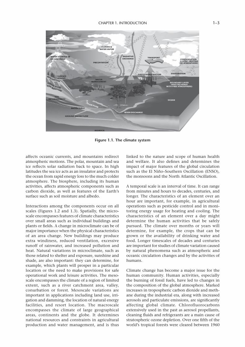
The climate system (Figure 1.1) is a complex, inter-active system consisting of the atmosphere, land surface, snow and ice, oceans and other bodies of water, and living organisms. The atmosphere is the gaseous envelope surrounding the Earth. The dry atmosphere consists almost entirely of nitrogen and oxygen, but also contains small quantities of argon, helium, carbon dioxide, ozone, methane and many other trace gases. The atmosphere also contains water vapour, condensed water droplets in the form of clouds, and aerosols. The hydrosphere is that part of the Earth’s climate system comprising liquid water distributed on and beneath the Earth’s surface in oceans, seas, rivers, freshwater lakes, underground reservoirs and other water bodies. The cryosphere collectively describes elements of the Earth system containing water in its frozen state and includes all snow and ice (sea ice, lake and river ice, snow cover, solid precipitation, glaciers, ice caps, ice sheets, permafrost and seasonally frozen ground). The surface lithosphere is the upper layer of the solid Earth, including both the continental crust and the ocean floor. The biosphere comprises all ecosystems and living organisms in the atmos-phere, on land (terrestrial biosphere) and in the oceans (marine biosphere), including derived dead organic matter, such as litter, soil organic matter and oceanic detritus.
Under the effects of solar radiation and the radia-tive properties of the surface, the climate of the Earth is determined by interactions among the components of the climate system. The interaction of the atmosphere with the other components plays a dominant role in forming the climate. The atmos-phere obtains energy directly from incident solar radiation or indirectly via processes involving the Earth’s surface. This energy is continuously redis-tributed vertically and horizontally through thermodynamic processes or large-scale motions with the unattainable aim of achieving a stable and balanced state of the system. Water vapour plays a significant role in the vertical redistribution of heat through condensation and latent heat transport. The ocean, with its vast heat capacity, limits the rate of temperature change in the atmosphere and supplies water vapour and sensible heat to the atmosphere. The distribution of the continents
CHAPTER 1. INTRODUCTION 1–3
affects oceanic currents, and mountains redirect atmospheric motions. The polar, mountain and sea ice reflects solar radiation back to space. In high latitudes the sea ice acts as an insulator and protects the ocean from rapid energy loss to the much colder atmosphere. The biosphere, including its human activities, affects atmospheric components such as carbon dioxide, as well as features of the Earth’s surface such as soil moisture and albedo.
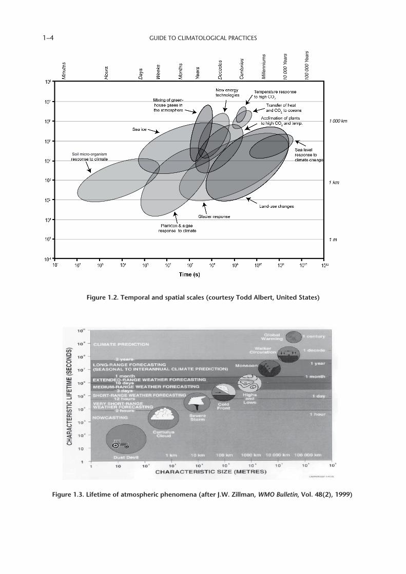
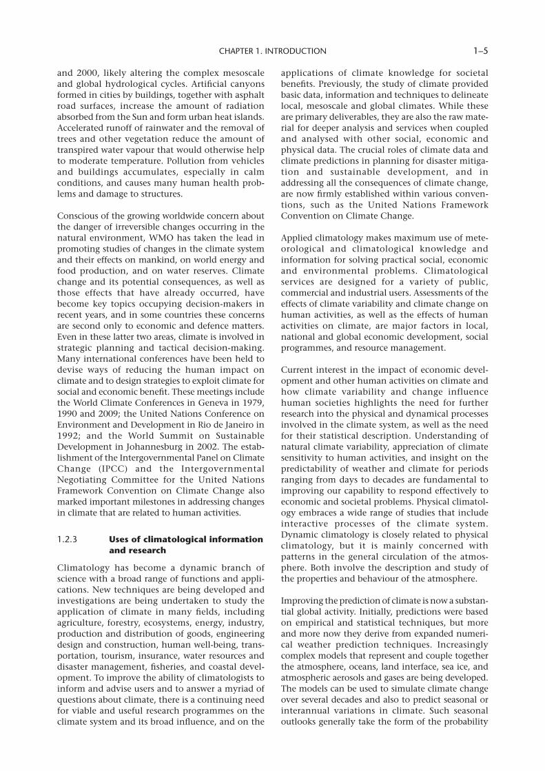
Interactions among the components occur on all scales (Figures 1.2 and 1.3). Spatially, the micro-scale encompasses features of climate characteristics over small areas such as individual buildings and plants or fields. A change in microclimate can be of major importance when the physical characteristics of an area change. New buildings may produce extra windiness, reduced ventilation, excessive runoff of rainwater, and increased pollution and heat. Natural variations in microclimate, such as those related to shelter and exposure, sunshine and shade, are also important: they can determine, for example, which plants will prosper in a particular location or the need to make provisions for safe operational work and leisure activities. The meso-scale encompasses the climate of a region of limited extent, such as a river catchment area, valley, conurbation or forest. Mesoscale variations are important in applications including land use, irri-gation and damming, the location of natural energy facilities, and resort location. The macroscale encompasses the climate of large geographical areas, continents and the globe. It determines national resources and constraints in agricultural production and water management, and is thus
linked to the nature and scope of human health and welfare. It also defines and determines the impact of major features of the global circulation such as the El Niño–Southern Oscillation (ENSO), the monsoons and the North Atlantic Oscillation.
A temporal scale is an interval of time. It can range from minutes and hours to decades, centuries, and longer. The characteristics of an element over an hour are important, for example, in agricultural operations such as pesticide control and in moni-toring energy usage for heating and cooling. The characteristics of an element over a day might determine the human activities that be safely pursued. The climate over months or years will determine, for example, the crops that can be grown or the availability of drinking water and food. Longer timescales of decades and centuries are important for studies of climate variation caused by natural phenomena such as atmospheric and oceanic circulation changes and by the activities of humans.
Climate change has become a major issue for the human community. Human activities, especially the burning of fossil fuels, have led to changes in the composition of the global atmosphere. Marked increases in tropospheric carbon dioxide and meth-ane during the industrial era, along with increased aerosols and particulate emissions, are significantly affecting global climate. Chlorofluorocarbons extensively used in the past as aerosol propellants, cleaning fluids and refrigerants are a main cause of stratospheric ozone depletion. Over one fifth of the world’s tropical forests were cleared between 1960
Figure.1 .1 ..The.climate.system
GUIDE TO CLIMATOLOGICAL PRACTICES 1–4
Figure 1.2. Temporal and spatial scales (courtesy Todd Albert, United States)
Mille
nniu
ms
10 0
00 Y
ears
100
000
Year
s
1 000 km
Soil micro-organism
-
Figure 1.3. Lifetime of atmospheric phenomena (after J.W. Zillman, WMO Bulletin, Vol. 48(2), 1999)
CHAPTER 1. INTRODUCTION 1–5
and 2000, likely altering the complex mesoscale and global hydrological cycles. Artificial canyons formed in cities by buildings, together with asphalt road surfaces, increase the amount of radiation absorbed from the Sun and form urban heat islands. Accelerated runoff of rainwater and the removal of trees and other vegetation reduce the amount of transpired water vapour that would otherwise help to moderate temperature. Pollution from vehicles and buildings accumulates, especially in calm conditions, and causes many human health prob-lems and damage to structures.
Conscious of the growing worldwide concern about the danger of irreversible changes occurring in the natural environment, WMO has taken the lead in promoting studies of changes in the climate system and their effects on mankind, on world energy and food production, and on water reserves. Climate change and its potential consequences, as well as those effects that have already occurred, have become key topics occupying decision-makers in recent years, and in some countries these concerns are second only to economic and defence matters. Even in these latter two areas, climate is involved in strategic planning and tactical decision-making. Many international conferences have been held to devise ways of reducing the human impact on climate and to design strategies to exploit climate for social and economic benefit. These meetings include the World Climate Conferences in Geneva in 1979, 1990 and 2009; the United Nations Conference on Environment and Development in Rio de Janeiro in 1992; and the World Summit on Sustainable Development in Johannesburg in 2002. The estab-lishment of the Intergovernmental Panel on Climate Change (IPCC) and the Intergovernmental Negotiating Committee for the United Nations Framework Convention on Climate Change also marked important milestones in addressing changes in climate that are related to human activities.
1.2.3 Usesofclimatologicalinformationandresearch
Climatology has become a dynamic branch of science with a broad range of functions and appli-cations. New techniques are being developed and investigations are being undertaken to study the application of climate in many fields, including agriculture, forestry, ecosystems, energy, industry, production and distribution of goods, engineering design and construction, human well-being, trans-portation, tourism, insurance, water resources and disaster management, fisheries, and coastal devel-opment. To improve the ability of climatologists to inform and advise users and to answer a myriad of questions about climate, there is a continuing need for viable and useful research programmes on the climate system and its broad influence, and on the
applications of climate knowledge for societal benefits. Previously, the study of climate provided basic data, information and techniques to delineate local, mesoscale and global climates. While these are primary deliverables, they are also the raw mate-rial for deeper analysis and services when coupled and analysed with other social, economic and physical data. The crucial roles of climate data and climate predictions in planning for disaster mitiga-tion and sustainable development, and in addressing all the consequences of climate change, are now firmly established within various conven-tions, such as the United Nations Framework Convention on Climate Change.
Applied climatology makes maximum use of mete-orological and climatological knowledge and information for solving practical social, economic and environmental problems. Climatological services are designed for a variety of public, commercial and industrial users. Assessments of the effects of climate variability and climate change on human activities, as well as the effects of human activities on climate, are major factors in local, national and global economic development, social programmes, and resource management.
Current interest in the impact of economic devel-opment and other human activities on climate and how climate variability and change influence human societies highlights the need for further research into the physical and dynamical processes involved in the climate system, as well as the need for their statistical description. Understanding of natural climate variability, appreciation of climate sensitivity to human activities, and insight on the predictability of weather and climate for periods ranging from days to decades are fundamental to improving our capability to respond effectively to economic and societal problems. Physical climatol-ogy embraces a wide range of studies that include interactive processes of the climate system. Dynamic climatology is closely related to physical climatology, but it is mainly concerned with patterns in the general circulation of the atmos-phere. Both involve the description and study of the properties and behaviour of the atmosphere.
Improving the prediction of climate is now a substan-tial global activity. Initially, predictions were based on empirical and statistical techniques, but more and more now they derive from expanded numeri-cal weather prediction techniques. Increasingly complex models that represent and couple together the atmosphere, oceans, land interface, sea ice, and atmospheric aerosols and gases are being developed. The models can be used to simulate climate change over several decades and also to predict seasonal or interannual variations in climate. Such seasonal outlooks generally take the form of the probability
GUIDE TO CLIMATOLOGICAL PRACTICES 1–6
that the value of an element, such as the mean temperature or aggregated rainfall over a period, will be above, near or below normal. Seasonal outlooks presently show skill for regions where there is a strong relationship between sea surface temperature and weather, such as in many tropical areas. Because of their probabilistic nature, however, much care is needed in their communication and application. Decision-making that incorporates climate informa-tion is a growing area of investigation.
All climate products and services, from information derived from past climate and weather data to esti-mations of future climate, for use in research, operations, commerce and government, are under-pinned by data obtained by extensively and systematically observing and recording a number of key variables that enable the characterization of climate on a wide range of timescales. The adequacy of a climate service is highly dependent on the spatial density and accuracy of the observations and on the data management processes. Without systematic observations of the climate system, there can be no climate services.
The need for more accurate and timely information continues to increase rapidly as the diversity of users’ requirements continues to expand. It is in the inter-est of every country to apply consistent practices in performing climate observations, in handling climate records and in maintaining the necessary quality and utility of the services provided.
1.3 INTERNATIONALCLIMATEPROGRAMMES
The WMO Commission for Climatology (CCl) is concerned with the overall requirements of WMO Members for advice, support and coordination in many climate activities. The Commission has been known by slightly different names and has seen its Terms of Reference change in accordance with changing demands and priorities, but it has effec-tively been in operation since it was established in 1929 under the International Meteorological Organization. It provides overall guidance for the implementation of the World Climate Programme within WMO. Additional details about interna-tional climate programmes are contained in Annex 2.
1.4 GLOBALANDREGIONALCLIMATEACTIVITIES
All countries should understand and provide for the climate-related information needs of the public.
This understanding requires climate observations, management and transmission of data, various data services, climate system monitoring, practical appli-cations and services for different user groups, forecasts on subseasonal and interannual time-scales, climate projections, policy-relevant assessments of climate variability and change, and research priorities that increase the potential bene-fits of all these activities. Many countries, especially the developing and least developed countries, may not have sufficient individual capacity to perform all of these services. The World Climate Conference-3 in Geneva in 2009 proposed the crea-tion of a Global Framework for Climate Services to strengthen the production, availability, delivery and application of science-based climate prediction and services. The Framework is intended to provide a mechanism for developers and providers of climate information, as well as climate-sensitive sectors around the world, to work together to help the global community better adapt to the chal-lenges of climate variability and change.
The World Meteorological Organization has devel-oped a network of Global Producing Centres for Long-Range Forecasts (GPCs) and Regional Climate Centres (RCCs) to assist Member countries cope effectively with their climate information needs. The definitions and mandatory functions of GPCs and RCCs are contained in the Manual on the Global Data-processing and Forecasting System (Volume I – Global Aspects, WMO-No. 485) and are part of the WMO Technical Regulations. The Manual also provides the criteria for the designation of GPCs, RCCs and other operational centres by WMO.
The designated GPCs produce global long-range fore-casts according to the criteria defined in the Manual on the Global Data-processing and Forecasting System and are recognized by WMO based on the recommen-dation of the Commission for Basic Systems. In addition, WMO has established the Lead Centre for Long-Range Forecast Multi-Model Ensembles and the Lead Centre for the Standardized Long-Range Forecast Verification System, which provide added value to the operational services of GPCs.
The Regional Climate Centres are designed to assist WMO Members in a given region to deliver better and more consistent climate services and products, such as regional long-range forecasts, and to strengthen the capability of Members to meet national climate information needs. The primary clients of an RCC are National Meteorological and Hydrological Services (NMHSs) and other RCCs in the region and in neighbouring areas. The services and products from the RCCs are provided to the NMHSs for further definition and dissemination and are not distributed to users without the permission of the NMHSs within the region. The responsibilities
CHAPTER 1. INTRODUCTION 1–7
of an RCC do not duplicate or replace those of NMHSs. It is important to note that NMHSs retain the mandate and authority to provide the liaison with national user groups and to issue advisories and warnings, and that all RCCs are required to adhere to the principles of WMO Resolution 40 concerning the exchange of data and products.
The complete suite of products and services of RCCs can vary from one region to another, based on the priorities established by the relevant Regional Association. There will, however, be certain essen-tial functions all WMO-designated RCCs must perform to established criteria, thus ensuring a certain uniformity of service around the globe in RCC mandatory functions. These functions include:(a) Operational activities for long-range forecast-
ing, including interpretation and assessment of relevant output products from GPCs, gener-ation of regional and subregional tailored products, and preparation of consensus state-ments concerning regional or subregional forecasts;
(b) Climate monitoring, including regional and subregional climate diagnostics, analysis of climate variability and extremes, and imple-mentation of regional Climate Watches for extreme climate events;
(c) Data services to support long-range forecast-ing, including the development of regional climate datasets;
(d) Training in the use of operational RCC prod-ucts and services.
In addition to these mandatory RCC functions, a number of activities are highly recommended. Some of these activities are downscaling of climate change scenarios, non-operational data services such as data rescue and data homogenization, coor-dination functions, training and capacity-building, and research and development.
Regional associations may also establish centres that conduct various climate functions as speci-fied in the Manual on the Global Data-processing and Forecasting System (Volume II – Regional Aspects). This volume does not fall under the WMO Technical Regulations, so these centres are not required to go through the formal designa-tion procedure. Regional associations have full responsibility for developing and approving the requirements for such centres. These centres often play an important participatory role in regional climate networks. It must be noted, however, that the term “WMO RCC” is reserved exclusively for those entities formally designated under Volume I – Global Aspects of the Manual on the Global Data-processing and Forecasting System, and therefore should not be used to refer to any other centre.
Recognizing that climate information can be of substantial benefit in adapting to and mitigating the impacts of climate variability and change, WMO has helped establish Regional Climate Outlook Forums. Using a predominantly consensus-based approach, the forums have an overarching responsibility to produce and disseminate a regional assessment of the state of the regional climate for the upcoming season. The forums bring together national, regional and interna-tional climate experts on an operational basis to produce regional climate outlooks based on input from NMHSs, regional institutions, RCCs and GPCs. They facilitate enhanced feedback from the users to climate scientists, and catalyse the development of user-specific products. They also review impediments to the use of climate infor-mation, share successful lessons regarding applications of past products and enhance sector-specific applications. The forums often lead to national forums for developing detailed national-scale climate outlooks and risk information, including warnings, for decision-makers and the public.
The Regional Climate Outlook Forum process, which can vary in format from region to region, typically includes at least the first of the following activities and, in some instances, all four:(a) Meetings of regional and international climate
experts to develop a consensus for regional climate outlooks, usually in a probabilistic form;
(b) A broader forum involving both climate scientists and representatives from user sectors, for the presentation of consensus climate outlooks, discussion and identifica-tion of expected sectoral impacts and impli-cations, and the formulation of response strategies;
(c) Training workshops on seasonal climate prediction to strengthen the capacity of national and regional climate scientists;
(d) Special outreach sessions involving media experts to develop effective communications strategies.
1.5 NATIONALCLIMATEACTIVITIES
In most countries, NMHSs have long held key responsibilities for national climate activities, including the making, quality control and storage of climate observations; the provision of climato-logical information; research on climate; climate prediction; and the applications of climate knowl-edge. There has been, however, an increasing contribution to these activities from academia and private enterprise.
GUIDE TO CLIMATOLOGICAL PRACTICES 1–8
Some countries have within their NMHSs a single division responsible for all climatological activities. In other countries the NMHS may find it beneficial to assign responsibilities for different climatological activities (such as observing, data management and research) to different units within the Service. The division of responsibilities could be made on the basis of commonality of skills, such as across synop-tic analysis and climate observation, or across research in weather and climate prediction. Some countries establish area or branch offices to handle subnational activities, while in other cases the necessary pooling and retention of skills for some activities are achieved through a regional coopera-tive entity serving the needs of a group of countries.
When there is a division of responsibility within an NMHS, or in those cases when responsibilities are assigned to another institution altogether, it is essential that a close liaison exist between those applying the climatological data in research or serv-ices and those responsible for the acquisition and management of the observations. This liaison is of paramount importance in determining the adequacy of the networks and of the content and quality control of the observations. It is also essen-tial that the personnel receive training appropriate to their duties, so that the climatological aspects are handled as effectively as would be the case in an integrated climate centre or division. If data are handled in several places, it is important to estab-lish a single coordinating authority to ensure that there is no divergence among datasets.
Climatologists within an NMHS should be directly accountable for, or provide consultation and advice regarding:(a) Planning of station networks;(b) Location or relocation of climatological
stations;(c) Care and security of the observing sites;(d) Regular inspection of stations;(e) Selection and training of observers;(f) Instruments or observing systems to be
installed so as to ensure that representative and homogeneous records are obtained (see Chapter 2).
Once observational data are acquired, they must be managed. Functions involved in the management of information from observing sites include data and metadata acquisition, quality control, storage, archiving and access (see Chapter 3). Dissemination of the collected climatic information is another requirement. An NMHS must be able to anticipate, investigate and understand the needs for climato-logical information among government departments, research institutions and academia, commerce, industry and the general public;
promote and market the use of the information; make available its expertise to interpret the data; and advise on the use of the data (see Chapter 6).
An NMHS should maintain a continuing research and development programme or establish working relationships with an institution that has research and development capabilities directly related to the climatological functions and operations of the NMHS. The research programme should consider new climate applications and products that increase user understanding and application of climate infor-mation. Studies should explore new and more efficient methods of managing an ever-increasing volume of data, improving user access to the archived data, and migrating data to digital form. Quality assurance programmes for observations and summa-ries should be routinely evaluated with the goal of developing better and timelier techniques. The use of information dissemination platforms such as the Internet should also be developed.
The meeting of national and international respon-sibilities, and the building of NMHS capacity relevant to climate activities, can be achieved only if adequately trained personnel are available. Thus, an NMHS should maintain and develop links with training and research establishments dealing with climatology and its applications. In particular, it should ensure that personnel attend training programmes that supplement general meteorolog-ical training with education and skills specific to climatology. The WMO Education and Training Programme fosters and supports international collaboration that includes the development of a range of mechanisms for continued training, such as fellowships, conferences, familiarization visits, computer-assisted learning, training courses and technology transfer to developing countries. In addition, other WMO Programmes, such as the World Climate Programme, the Hydrology and Water Resources Programme and the Agricultural Meteorology Programme, undertake capacity-building activities relevant to climate data, monitoring, prediction, applications and services.
To be successful, a national climate services programme must have a structure that works effec-tively within a particular country. The structure must be one that allows the linkage of available applications, scientific research, technological capabilities and communications into a unified system. The essential components of a national climate services programme are:(a) Mechanisms to ensure that the climate infor-
mation and prediction needs of all users are recognized;
(b) Collection of meteorological and related observations, management of databases and the provision of data;
CHAPTER 1. INTRODUCTION 1–9
(c) Coordination of meteorological, oceano-graphic, hydrological and related scientific research to improve climate services;
(d) Multidisciplinary studies to determine national risk and sectoral and community vulnerability related to climate variability and change, to formulate appropriate response strategies, and to recommend national policies;
(e) Development and provision of climate infor-mation and prediction services to meet user needs;
(f) Linkages to other programmes with similar or related objectives to avoid unnecessary dupli-cation of efforts.
It is important to realize that a national climate serv-ices programme constitutes an ongoing process that may change in structure through time. An integral part of this process is the continual review and incor-poration of user requirements and feedback in order to develop useful products and services. Gathering requirements and specifications is vital in the proc-ess of programme development. Users may contribute through the evaluation of products, which invariably leads to refinements and the devel-opment of improved products. Measuring the benefits of the application of products can be a diffi-cult task, but interaction with users through workshops, training and other outreach activities will aid the process. The justification for a national climate services programme, or requests for interna-tional financial support for aspects of the programme, can be greatly strengthened by well-documented user requirements and positive feedback. The docu-mented endorsement of the programme, by one or more representative sections of the user community, is essential to guide future operations and to assist in the promotion of the service as a successful entity.
1.6 REFERENCES
1.6.1 WMOpublications
Global Climate Observing System (GCOS), 2004: Implementation Plan for the Global Observing System for Climate in Support of the UNFCCC (WMO/TD-No. 1219, GCOS-No. 92), Geneva.
Integrated Global Observing Strategy (IGOS), 2007: Cryosphere Theme Report: For the Monitoring of our Environment from Space and from Earth (WMO/TD-No. 1405), Geneva.
Intergovernmental Panel on Climate Change (IPCC), 2004: 16 Years of Scientific Assessment in Support of the Climate Convention, Geneva.
———, 2007: The Fourth Assessment Report: Climate Change 2007 (AR4), Vols. 1–4. Cambridge, Cambridge University Press.
World Climate Research Programme (WCRP), 2005: The World Climate Research Programme Strategic Framework 2005–2015. Coordinated Observation and Prediction of the Earth System (WMO/TD-No. 1291, WCRP-No. 123), Geneva.
World Meteorological Organization, 1983: Guide to Climatological Practices. Second edition (WMO-No. 100), Geneva.
———, 1986: Report of the International Conference on the Assessment of the Role of Carbon Dioxide and of Other Greenhouse Gases in Climate Variations and Associated Impacts (Villach, Austria, 9–15 October 1985) (WMO-No. 661), Geneva.
———, 1990: Forty Years of Progress and Achievement: A Historical Review of WMO (Sir Arthur Davies, ed.) (WMO-No. 721), Geneva.
———, 1990: The WMO Achievement: 40 Years in the Service of International Meteorology and Hydrology (WMO-No. 729), Geneva.
———, 1991: Manual on the Global Data-processing System. Vol. I – Global Aspects. Supplement No. 10, October 2005 (WMO-No. 485), Geneva.
———, 1992: International Meteorological Vocabulary (WMO-No. 182), Geneva.
———, 1992: Manual on the Global Data-processing System. Vol. II – Regional Aspects. Supplement No. 2, August 2003 (WMO-No. 485), Geneva.
———, 1997. Report of the GCOS/GOOS/GTOS Joint Data and Information Management Panel, Third session (Tokyo, Japan, 15–18 July 1997) (WMO/TD-No. 847, GCOS-No. 39, GOOS- No. 11, GTOS-No. 11), Geneva.
———, 2003: Climate: Into the 21st Century. Cambridge, Cambridge University Press.
———, 2008: Final Report of the CCl/CBS Intercommission Technical Meeting on Designation of Regional Climate Centres (Geneva, 21–22 January 2008), Geneva.
———, 2000: WMO – 50 Years of Service (WMO-No. 912), Geneva.
———, 2009: WMO Statement on the Status of the Global Climate in 2008 (WMO-No. 1039), Geneva.
———, 2003: Proceedings of the Meeting on Organization and Implementation of Regional Climate Centres (Geneva, 27–28 November 2003) (WMO/TD- No. 1198, WCASP-No. 62), Geneva.
———, 2004. Implementation Plan for the Global Observing System for Climate in support of the UNFCCC (WMO/TD-No. 1219, GCOS-No. 92), Geneva.
1.6.2 Additionalreading
Aristotle, circa 350 B.C.: Meteorologica.Bergeron, T., 1930: Richtlinien einer dyna-
mischen Klimatologie. Meteorologische Zeitung, 47:246–262.
Federov, E.E., 1927: Climate as totality of the weather. Monthly Weather Rev., 55:401–403.
GUIDE TO CLIMATOLOGICAL PRACTICES 1–10
Geiger, R., 1927: Das Klima der bodennahen Luftschicht. Ein Lehrbuch der Mikroklimatologie. Second edition, 1942; third edition, 1942; fourth edition, 1961. Braunschweig, Vieweg.
Geiger, R., R.H. Aron and P. Todhunter, 2003. The Climate Near the Ground. Sixth edition. Lanham, Maryland, Rowman and Littlefield Publishers.
Group on Earth Observations (GEO), 2007: GEO 2007-2009 Work Plan. Toward Convergence, Geneva.
———, 2005: Global Earth Observation System of Systems (GEOSS): 10-year Implementation Plan. Reference Document GEO 1000R/ESA SP-1284. Noordwijk, European Space Agency Publications Division, ESTEC.
Hadley, G., 1735: Concerning the cause of the general trade-winds. Royal Soc. London Philos. Trans., 29:58–62.
Hann, J. von, 1883: Handbuch der Klimatologie. Second edition, 1897, 3 vols.; third edition, 1908–11, 3 vols. Stuttgart, Englehorn.
Hippocrates, circa 400 B.C.: On Airs, Waters, and Places.Köppen, W. and G. Geiger (eds.), 1930–1939.
Handbuch der Klimatologie, 5 vols. Berlin, Gebruder Borntraeger.
Köppen, W., 1918: Klassification der Klimate nach Temperatur, Niederschlag and Jahreslauf. Petermanns Geog. Mitt., 64:193–203, 243–248.
Landsberg, H., 1962: Physical Climatology. Second edition. Dubois, Pennsylvania, Gray Printing.
Mann, M.E., Bradley, R.S. and M.K. Hughes, 1999: Northern Hemisphere temperatures during the past millennium: Inferences, uncertain-ties, and limitations. Geophys. Res. Lett., 26(6):759.
Thornthwaite, C.W., 1948. An Approach toward a rational classification of climate. Geographical Rev., 38(1):55–94.
Walker, G.T., 1923-24: World weather, I and II. Indian Meteorol. Dept. Mem., 24(4):9.
.
CLIMATE.OBSERVATIONS,.STATIONS.AND.NETWORKS
CHAPTER 2
2.1 INTRODUCTION
All national climate activities, including research and applications, are primarily based on observations of the state of the atmosphere or weather. The Global Observing System provides observations of the state of the atmosphere and ocean surface. It is operated by National Meteorological and Hydrological Services, national or international satellite agencies, and several organizations and consortiums dealing with specific observing systems or geographic regions. The WMO Global Observing System is a coordinated system of different observing subsystems that provides in a cost-effective way high-quality, standardized meteorological and related environmental and geophysical observations, from all parts of the globe and outer space. Examples of the observing subsystems relevant to climate are the Global Climate Observing System (GCOS) Surface Network (GSN), the GCOS Upper-Air Network (GUAN), Regional Basic Climatological Networks, Global Atmosphere Watch (GAW), marine observing systems, and the satellite-based Global Positioning System. The observations from these networks and stations are required for the timely preparation of weather and climate analyses, forecasts, warnings, climate services, and research for all WMO Programmes and relevant environmental programmes of other international organizations.
This chapter on observations follows the sequence of specifying the elements needed to describe the climate and the stations at which these elements are measured, instrumentation, siting of stations, network design and network operations. The guid-ance is based on the WMO Guide to Meteorological Instruments and Methods of Observation (WMO-No. 8, fifth, sixth and seventh editions), the Guide to the Global Observing System (WMO-No. 488) and the Guidelines on Climate Observation Networks and Systems (WMO/TD-No. 1185). Each edition of the Guide to Meteorological Instruments and Methods of Observation has a slightly different emphasis. For example, the sixth edition contains valuable infor-mation on sensor calibration, especially of the basic instrumentation used at climate stations, but Tables 2 and 3 of the fifth edition provide more informa-tion about the accuracy of measurements that are needed for general climatological purposes. Cross references are provided in the sections below to other WMO publications containing more detailed guidance.
Guidance is also based on ten climate monitoring principles set forth in the Report of the GCOS/GOOS/GTOS Joint Data and Information Management Panel (Third Session, Tokyo, 15–18 July 1997, WMO/TD- No. 847): 1. The impact of new systems or changes to
existing systems should be assessed prior to implementation.
2. A suitable period of overlap for new and old observing systems is required.
3. The details and history of local conditions, instruments, operating procedures, data processing algorithms, and other factors perti-nent to interpreting data (metadata) should be documented and treated with the same care as the data themselves.
4. The quality and homogeneity of data should be regularly assessed as a part of routine operations.
5. Consideration of the needs for environmental and climate monitoring products and assess-ments should be integrated into national, regional, and global observing priorities.
6. Operation of historically uninterrupted stations and observing systems should be maintained.
7. High priority for additional observations should be focused on data-poor areas, poorly observed parameters, areas sensitive to change, and key measurements with inad-equate temporal resolution.
8. Long-term requirements should be specified to network designers, operators, and instru-ment engineers at the outset of system design and implementation.
9. The conversion of research observing systems to long-term operations in a carefully planned manner should be promoted.
10. Data management systems that facilitate access, use, and interpretation of data and products should be included as essential elements of climate monitoring systems.
These principles were established primarily for surface-based observations, but they also apply to data for all data platforms. Additional principles specifically for satellite observations are listed in section 2.3.4.
2.2 CLIMATICELEMENTS
A climatic element is any one of the properties of the climate system described in section 1.2.2. Combined
GUIDE TO CLIMATOLOGICAL PRACTICES 2–2
with other elements, these properties describe the weather or climate at a given place for a given period of time. Every meteorological element that is observed may also be termed a climatic element. The most commonly used elements in climatology are air temperature (including maximum and mini-mum), precipitation (rainfall, snowfall and all kinds of wet deposition, such as hail, dew, rime, hoar frost and precipitating fog), humidity, atmospheric motion (wind speed and direction), atmospheric pressure, evaporation, sunshine, and present weather (for example, fog, hail and thunder). Properties of the land surface and subsurface (including hydro-logical elements, topography, geology and vegetation), of the oceans, and of the cryosphere are also used to describe climate and its variability.
The subsections below describe commonly observed elements for specific kinds of stations and networks of stations. Details are in the Manual on the Global Observing System, the WMO Technical Regulations (WMO-No. 49, in particular Volume III – Hydrology), and the Guide to Agricultural Meteorological Practices (WMO-No. 134). These documents should be kept readily available and consulted as needed.
2.2.1 Surfaceandsubsurfaceelements
An ordinary climatological station provides the basic land area requirements for observing daily maximum and minimum temperature and amount of precipitation. A principal climatological station usually provides a broader range of observations of weather, wind, cloud characteristics, humidity, temperature, atmospheric pressure, precipitation, snow cover, sunshine and solar radiation. In order to define the climatology of precipitation, wind, or any other specific element, it is sometimes neces-sary to operate a station to observe one or a subset of these elements, especially where the topography is varied. Reference climatological stations (see section 2.5) provide long-term, homogeneous data for the purpose of determining climatic trends. It is desirable to have a network of these stations in each country, representing key climate zones and areas of vulnerability.
In urban areas weather can have a significant impact. Heavy rains can cause severe flooding; snow and freezing rain can disrupt transportation systems; and severe storms with accompanying lightning, hail and high winds can cause power fail-ures. High winds can also slow or stop the progress of automobiles, recreational vehicles, railcars, tran-sit vehicles and trucks. The urban zone is especially susceptible to land falling tropical storms because of the large concentrations of people at risk, the high density of man-made structures, and the increased risk of flooding and contamination of potable water supplies. Urban stations usually
observe the same elements as principal climatologi-cal stations, with the addition of air pollution data such as low-level ozone and other chemicals and particulate matter.
Marine observations can be generally classified into physical-dynamical and biochemical elements. The physical-dynamical elements (such as wind, tempera-ture, salinity, wind and swell waves, sea ice, ocean currents and sea level) play an active role in changing the marine system. The biochemical elements (such as dissolved oxygen, nutrients and phytoplankton biomass) are generally not active in the physical-dynamical processes, except perhaps at long timescales, and thus are called passive elements. From the perspective of most NMHSs, high priority should generally be given to the physical-dynamical elements, although in some cases biochemical elements could be important when responding to the needs of stakeholders (for example, observations related to the role of carbon dioxide in climate change).
In some NMHSs with responsibilities for monitor-ing hydrological events, hydrological planning, or hydrological forecasting and warning, it is neces-sary to observe and measure elements specific to hydrology. These elements may include combina-tions of river, lake and reservoir level; streamflow; sediment transport and deposition; rates of abstrac-tion and recharge; water and snow temperatures; ice cover; chemical properties of water; evapora-tion; soil moisture; groundwater level; and flood extent. These elements define an integral part of the hydrologic cycle and play an important role in the variability of climate.
In addition to surface elements, subsurface elements such as soil temperature and moisture are particu-larly important for application to agriculture, forestry, land-use planning and land-use manage-ment. Other elements that should be measured to characterize the physical environment for agricul-tural applications include evaporation from soil and water surfaces, sunshine, short- and long-wave radiation, plant transpiration, runoff and water table, and weather observations (especially hail, lightning, dew and fog). Ideally, measurements of agriculturally important elements should be taken at several levels between 200 cm below the surface and 10 m above the surface. Consideration should also be given to the nature of crops and vegetation when determining the levels.
Proxy data are measurements of conditions that are indirectly related to climate, such as phenology, ice core samples, varves (annual sediment deposits), coral reefs and tree ring growth. Phenology is the study of the timing of recurring biological events in the animal and plant world, the causes of their
CHAPTER 2. CLIMATE OBSERVATIONS, STATIONS AND NETWORKS 2–3
timing with regard to biotic and abiotic forces, and the interrelation among phases of the same or different species. Leaf unfolding, flowering of plants in spring, fruit ripening, colour changing and leaf fall in autumn, as well as the appearance and depar-ture of migrating birds, animals and insects are all examples of phenological events. Phenology is an easy and cost-effective system for the early detec-tion of changes in the biosphere and therefore complements the instrumental measurements of national meteorological services very well.
An ice core sample contains snow and ice and trapped air bubbles. The composition of a core, especially the presence of hydrogen and oxygen isotopes, relates to the climate of the time the ice and snow were deposited. Ice cores also contain inclusions such as windblown dust, ash, bubbles of atmospheric gas, and radioactive substances in the snow deposited each year. Various measurable properties along the core profiles provide proxies for temperature, ocean volume, precipitation, chemistry and gas composition of the lower atmos-phere, volcanic eruptions, solar variability, sea surface productivity, desert extent and forest fires. The thickness and content of varves are similarly related to annual or seasonal precipitation, stream-flow, and temperature.
Tropical coral reefs are very sensitive to changes in climate. Growth rings relate to the temperature of the water and to the season in which the rings grew. Analysis of the growth rings can match the water temperature to an exact year and season. Data from corals are used to estimate past El Niño–Southern Oscillation (ENSO) variability, equatorial upwelling, changes in subtropical gyres, trade wind regimes and ocean salinity.
Tree-ring growth shows great interannual variability and also large spatial differences. Some of the varia-tion can be related to weather and climate conditions in the microscale and macroscale; plants can be viewed as integrative measurement devices for the environment. Since trees can live for centuries, annual growth rings in some tree species can provide a long historical indication (predating instrumental measurements) of climate variability. Because of the close relationship between plant development and weather and climate, phenological observation networks are run by the NMHSs in many countries.
Table 2.1 summarizes the most common surface and subsurface climatic elements that are observed for various networks or types of station.
2.2.2 Upper-airelements
Upper-air observations are an integral component of the Global Observing System. The spectrum of
climate activities that require upper-air observations includes monitoring and detecting climate variabil-ity and change, climate prediction on all timescales, climate modelling, studies of climate processes, data reanalysis activities, and satellite studies concerning calibration of satellite retrievals and radiative transfer.
The longest record of upper-air observations has been obtained from balloon-based instruments combined with ground tracking devices in a radio-sonde network. These radiosonde measurements provide a database of atmospheric variables dating back to the 1930s, although coverage is generally poor before 1957. The radiosonde data record is characterized by many discontinuities and biases resulting from instrument and operational proce-dural changes and incomplete metadata. Satellite observations have been available since the 1970s, and some have been assembled and reprocessed to create continuous records. Just as the radiosonde record has deficiencies, however, the satellite data also suffer from, among other things, limited verti-cal resolution, orbit drift, satellite platform changes, instrument drift, complications with calibration procedures, and the introduction of biases through modifications of processing algorithms. Other upper-air measurements have come from moving platforms such as aircraft. Observations from some high-mountain locations have also been consid-ered part of the upper-air measurement system.
The main observational requirements for monitor-ing long-term upper-air changes are:(a) A long-term (multidecadal), stable, temporally
homogeneous record so that changes can confi-dently be identified as true atmospheric changes rather than changes in the observing system or as artefacts of homogenization methods;
(b) Good vertical resolution to describe the verti-cal structure of temperature, water vapour, and ozone changes, and of changes in the tropopause;
(c) Sufficient geographical coverage and resolu-tion, so that reliable global and area trends can be determined;
(d) Observational precision finer than the expected atmospheric variations to allow clear identification of both variability and long-term changes. This requirement is particularly important for water vapour observations in the upper troposphere and stratosphere.
The essential climate elements from upper-air observations are given in the Second Report on the Adequacy of the Global Observing Systems for Climate in Support of the UNFCCC (WMO/TD-No. 1143) and the Implementation Plan for the Global Observing System for Climate in Support of the UNFCCC
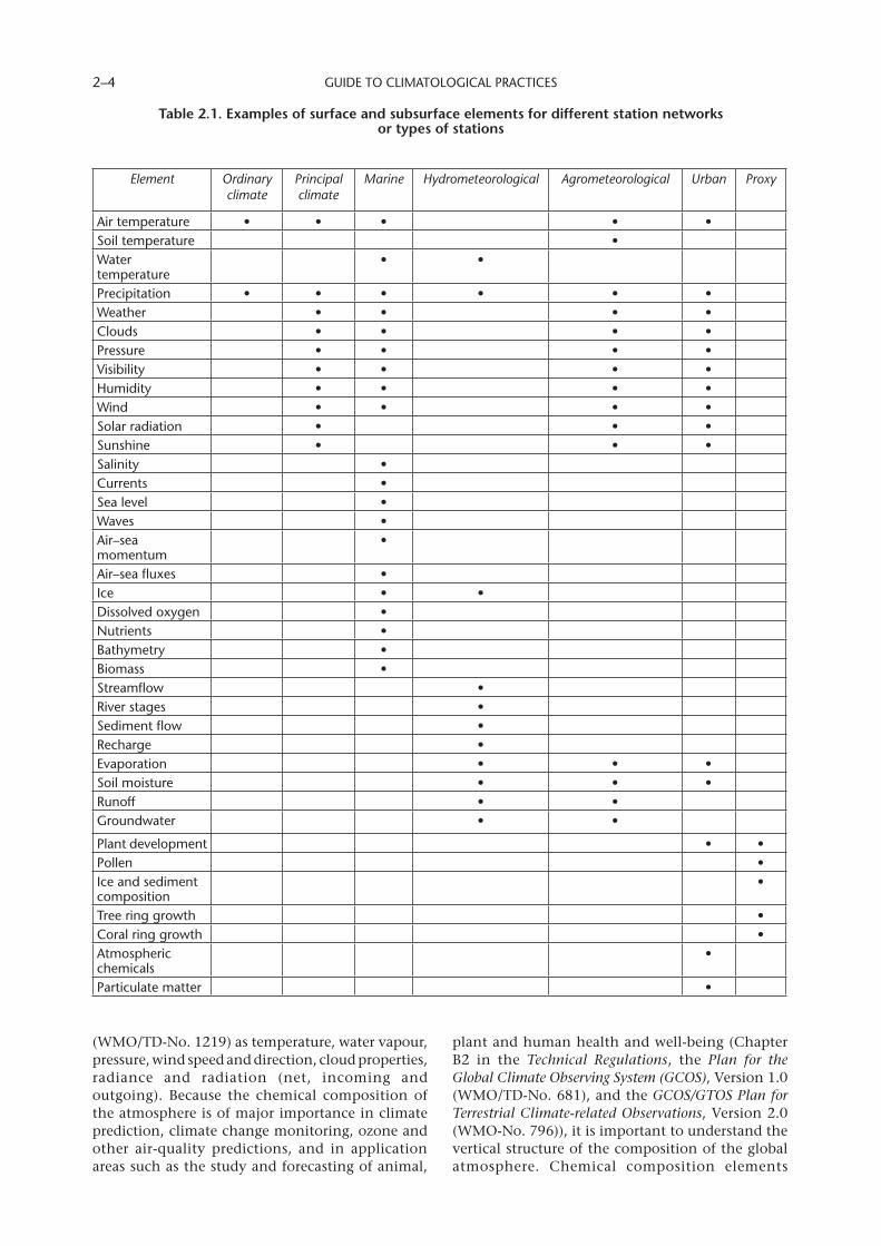
GUIDE TO CLIMATOLOGICAL PRACTICES 2–4
Element Ordinary climate
Principal climate
Marine Hydrometeorological Agrometeorological Urban Proxy
Air temperature • • • • •Soil temperature •Water temperature
• •
Precipitation • • • • • •Weather • • • •Clouds • • • •Pressure • • • •Visibility • • • •Humidity • • • •Wind • • • •Solar radiation • • •Sunshine • • •Salinity •Currents •Sea level •Waves •Air–sea momentum
•
Air–sea fluxes •Ice • •Dissolved oxygen •Nutrients •Bathymetry •Biomass •Streamflow •River stages •Sediment flow •Recharge •Evaporation • • •Soil moisture • • •Runoff • •Groundwater • •
Plant development • •Pollen •Ice and sediment composition
•
Tree ring growth •Coral ring growth •Atmospheric chemicals
•
Particulate matter •
(WMO/TD-No. 1219) as temperature, water vapour, pressure, wind speed and direction, cloud properties, radiance and radiation (net, incoming and outgoing). Because the chemical composition of the atmosphere is of major importance in climate prediction, climate change monitoring, ozone and other air-quality predictions, and in application areas such as the study and forecasting of animal,
plant and human health and well-being (Chapter B2 in the Technical Regulations, the Plan for the Global Climate Observing System (GCOS), Version 1.0 (WMO/TD-No. 681), and the GCOS/GTOS Plan for Terrestrial Climate-related Observations, Version 2.0 (WMO-No. 796)), it is important to understand the vertical structure of the composition of the global atmosphere. Chemical composition elements
Table.2 .1 ..Examples.of.surface.and.subsurface.elements.for.different.station.networks..or.types.of.stations
CHAPTER 2. CLIMATE OBSERVATIONS, STATIONS AND NETWORKS 2–5
requiring measurement both in the free atmosphere and near the ground include concentrations of ozone and other greenhouse gases, such as carbon dioxide and methane, atmospheric turbidity (aerosol optical depth), aerosol total load, reactive gas species, and radionuclides. Measurements of acid rain (or more generally precipitation and particulate chemistry) and ultraviolet radiation are also needed. (See the Integrated Global Atmospheric Chemistry Observations (IGACO) Report of IGOS-WMO-ESA (WMO/TD-No. 1235) for details concerning the chemical composition of the atmosphere).
Upper-air measurements should capture the full range of climate regimes and surface types. Radiative transfer codes used to convert raw satellite radiances to geophysical parameters depend upon assump-tions about the surface conditions. Therefore, different local environmental conditions should be represented, including both land and ocean areas.
2.2.3 Elementsmeasuredbyremote-sensing
Satellites and other remote-sensing systems such as weather radar provide an abundance of additional information, especially from otherwise data-sparse areas, but are not as yet capable of providing, with the required accuracy and homogeneity, measure-ments of many of the elements that are reported from land-based surface stations. The spatial cover-age they offer makes them complementary to, but not a substitute for, the surface networks. The elements that can be measured or estimated remotely are precipitation (with limited accuracy over small areas, ocean–atmosphere interfaces, highlands or steep orography); cloud amount; radi-ation fluxes; radiation budget and albedo; upper oceanic biomass, ocean surface topography and wave height; sea-ice cover; sea surface temperature; ocean surface wind vectors and wind speed; atmos-pheric temperature, humidity and wind profiles; chemical constituents of the atmosphere; snow cover; ice sheet and glacier extent; vegetation and land cover; and land surface topography.
Greater spatial and temporal coverage can be achieved with remote-sensing than with in situ observations. Remotely sensed data also supplement observations from other platforms and are especially useful when observations from other platforms are missing or corrupted. Although this is an advantage, there are problems in using remotely sensed data directly for climate applications. Most importantly, the short period of record means that remotely sensed data cannot be used to infer long-term climate variability and change. Also, remotely sensed data may not be directly comparable to in situ measurements. For example, satellite estimates
of the Earth’s skin temperature are not the same as temperature measurements taken in a standard screen, and the relationship between radar measurements of reflectivity and precipitation amounts collected in raingauges may be quite complex. It is possible with care, however, to construct homogeneous series that combine remotely sensed and in situ measurements.
2.3 INSTRUMENTATION
Climatological stations that are part of a national network should be equipped with standard approved instruments; the NMHS may supply the instruments. When equipment is supplied by other agencies or purchased by the observer, every effort should be made by a climate office to ensure compli-ance with national standards.
This section gives guidance on some basic surface instrumentation and on the selection of instru-ments. There are several other WMO publications that are necessary companions to this Guide, and should be readily available and consulted as needed. A thorough survey of instruments suitable for meas-uring climate and other elements at land and marine stations is provided in the Guide to Meteorological Instruments and Methods of Observation. Details of instrumentation needed for the measure-ment of chemical composition are given in the International Operations Handbook for Measurement of Background Atmospheric Pollution (WMO-No. 491), for agrometeorological elements in the Guide to Agricultural Meteorological Practices, and for hydro-logical purposes in the Guide to Hydrological Practices (WMO-No. 168).
When selecting instrumentation, including any associated data-processing and transmission systems, the 10 climate monitoring principles (section 2.1) should be followed. Several concerns should be considered when complying with these principles:(a) Reliability;(b) Suitability for the operational environment at
the station of use;(c) Accuracy;(d) Simplicity of design;(e) Reasons for taking observations.
Reliability requires that an instrument functions within its design specifications at all times. Unreliable instrumentation leads to data gaps, biases and other inhomogeneities. Reliable instru-ments need to be robust enough to cope with the full range of weather and physical extremes expected at the site, and possibly the handling that is part of manual observations.
GUIDE TO CLIMATOLOGICAL PRACTICES 2–6
Instruments must be suited both to the climate in which they must function, and to other equip-ment with which they must operate. For example, an anemometer head at a cold location will need to withstand icing, while one in a desert area will need to be protected against dust ingression. Sensors for use in an automatic weather station need to provide output suitable for automatic processing. The standard mercury-in-glass ther-mometer used at a manual recording site, for example, will need to be substituted by a tempera-ture-sensitive probe, such as a thermocouple, whose response can be converted into an elec-tronic signal. Instruments must also be sited so that they can be accessed and maintained.
Ideally, all instruments should be chosen to provide the high level of accuracy and precision required for climatological purposes. It is also important that the instrument can continue to provide the required level of accuracy for a long period of time, as instru-ment “drift” can lead to serious inhomogeneities in a climate record; accuracy is of limited use without reliability.
The simpler the instrumentation, the easier it is to operate and to maintain, and the easier it is to monitor its performance. It is sometimes necessary to install redundant sensors (for example, triple thermistors at automated data-logger stations) to properly track performance and reliability over time. Complex systems can easily lead to data inho-mogeneities, data loss, high maintenance cost and changing accuracy.
The purpose of the observations generally dictates requirements for measurements. Types of instru-ments, installation of sensors, and characteristics of the instruments should be considered to ensure that measurement requirements can be met.
Details about these concerns, including instru-ment and measurement standards and recommended practices, are can be found in the Guide to Meteorological Instruments and Methods of Observation.
2.3.1 Basicsurfaceequipment
There may be a variety of options for obtaining climate observations from surface stations. These options include equipping a station with, for exam-ple, basic instruments, autographic or automated output available for unmanned periods, or totally automated sensors. When considering the options, it is important to compare costs of personnel, main-tenance and replacement. Price negotiation is often possible with manufacturers on the basis of, for example, quantities purchased, among other things.
Whenever possible, trained local personnel, such as a caretaker, should examine an observing site on a regular basis to keep surface conditions (such as grass growth) in check, perform basic mainte-nance of instruments (such as simple cleaning), examine for damage, and detect breaches of secu-rity. These tasks should be performed at least weekly at accessible, manned land stations. Inspection of sites and instruments at remote locations should be made as often as possible. Personnel should also be available to provide rapid maintenance response when critical systems fail.
Autographic and data-logger equipment exists for the recording of many climatic elements, such as temperature, humidity, wind and rates of rainfall. Data need to be transferred from autographic records to tables or digital form. Observers should ensure that the equipment is operating properly and that information recorded on charts, for example, is clear and distinct. Observers should be responsible for regularly verifying and evaluating the recorded data (by checking against direct-reading equipment) and for making time marks at frequent, specified intervals. The recorded data can be effectively used to fill gaps and to complete the record when direct observations are missed because of illness and other causes of absence from the observing station. Sections 1.4.2 and 1.4.3 of the Guide to Meteorological Instruments and Methods of Observation (fifth edition) give specific guidance on the maintenance and operation of recording instruments, drums and clocks.
Data from automatic weather stations (AWSs), at which instruments record and transmit observa-tions automatically, are usually restricted to those readily obtained in digital form, although the range of sensors is wide and continues to evolve. Such stations have been used to supplement manned stations and to increase network densities, report-ing frequencies and the quantities of elements observed, especially in remote and largely unpopu-lated areas where human access is difficult. Some of the sensitivity and accuracy requirements of these automated stations are given in the Guide to Meteorological Instruments and Methods of Observation; others are being developed, especially for studies of climate variability.
In many countries, AWSs have lowered operational costs. NMHSs choosing between manned and AWS observation programmes need to consider a number of issues. Notwithstanding the considerable poten-tial for AWSs to provide high-frequency data, as well as additional data from remote locations, there are several significant costs associated with operat-ing an AWS, including labour costs for maintenance and ensuring AWS reliability, labour availability,
CHAPTER 2. CLIMATE OBSERVATIONS, STATIONS AND NETWORKS 2–7
accessibility for installation and maintenance, the availability of suitable power sources, security of the site, and communications infrastructure. These aspects must be carefully weighed against the significant benefits, such as a denser or more exten-sive network. AWSs can be powerful alternatives to manned observational programmes and sometimes are the only option, but they require a strong organizational commitment to manage them.
Marine instrumentation includes drifting and moored data buoys, ice floats and subsurface floats. Although the data are collected remotely, the instruments are generally performing in situ meas-urements. They are a cost-effective means for obtaining meteorological and oceanographic data from remote ocean areas. As such, they form an essential component of marine observing systems and meteorological and oceanographic operational and research programmes. For example, the Tropical Atmosphere Ocean array of moorings has enabled timely collection of high-quality oceanographic and surface meteorological data across the equato-rial Pacific Ocean for the monitoring, forecasting and understanding of climate swings associated with El Niño and La Niña.
2.3.2 Upper-airinstruments
Historically, most climatological data for the upper air have been derived from measurements made for synoptic forecasting by balloon-borne radiosondes. A variety of techniques and instruments are used for the measurement of pressure, temperature, humidity and wind, and for processing instrumen-tal output into meteorological quantities. It is important for each NMHS to issue suitable instruc-tion manuals to each upper-air station for the proper use of equipment and interpretation of data. The Manual on the Global Observing System (WMO-No. 544, section 2.10.4.5) requires that prompt reports be made to the WMO Secretariat of changes in radiosonde type or changes in wind systems in operational use at a station.
There are several issues concerning the quality of radiosonde measurements for climate monitoring and climate change detection purposes. Radiation errors cause uncertainties in temperature. Standard radiosondes are not capable of measuring water vapour at low temperatures with sufficient accu-racy. Sensor types, especially humidity sensors, have changed over time. The spatial coverage of radiosonde observations is not uniform; most stations are located on the land-surface territories of the northern hemisphere, while the southern hemisphere and ocean networks are much less dense. The historical record of radiosonde observa-tions has innumerable problems relating to a lack of intercomparisons among types of radiosondes
and sensor and exposure differences; metadata concerning instrumentation, data-reduction and data-processing procedures are crucial to utilizing radiosonde data in climate applications. New refer-ence radiosondes are being developed to mitigate the deficiencies of the current standard radio-sondes. A limited network of these will be used to calibrate and validate various satellite observations of both temperature and water vapour.
An upper-air observing system may change over time with technological advances. Hence, a key requirement of the network is sufficient overlap of systems to maintain continuity and allow full comparison of the accuracy and precision of the old and new systems. Measurement systems should be calibrated regularly at the site. It is imperative that instrument replacement strategies take into account changes in other networks, such as the use of satel-lites. The Climate Monitoring Principles (see section 2.1) should guide the development and operation of an upper-air observing system.
2.3.3 Surface-basedremote-sensing
Remote-sensing can use either active or passive sensors. Active sensor systems emit some form of radiation, which is scattered by various targets; the sensors detect the backscatter. Passive sensors meas-ure radiation being emitted (or modified) by the environment.
The most common surface-based active remote-sensing technique is weather radar. A short pulse of high-power microwave energy is focused by an antenna system into a narrow beam. This beam is scattered back by the target precipitation, with the backscattered radiation received, generally, by the same antenna system. The location of the precipi-tation can be determined from the azimuth and elevation of the antenna and the time between transmitting and receiving the reflected energy. The power of the received radiation depends on the nature of the precipitation, and the signal can be processed to estimate its intensity. Atmospheric and environmental conditions can adversely affect radar data, and caution should be exercised when interpreting the information. Some of these effects include returns from mountains, buildings, and other non-meteorological targets; attenuation of the radar signal when viewing weather echoes through intervening areas of intense precipita-tion; temperature inversions in the lower layers of the atmosphere, which bend the radar beam in such a way that ground clutter is observed where normally not expected; and the bright band, which is a layer of enhanced reflectivity caused by the melting of ice particles as they fall through the freezing level in the atmosphere, which can result in overestimation of rainfall. Use of radar data in
GUIDE TO CLIMATOLOGICAL PRACTICES 2–8
climate studies has been limited by access and processing capabilities, uncertainties in calibra-tion and calibration changes, and the complex re lat ionship between ref lect ivi ty and precipitation.
Wind profilers use radar to construct vertical profiles of horizontal wind speed and direction from near the surface to the tropopause. Fluctuations of atmospheric density are caused by turbulent mixing of air with different temperatures and mois-ture content. Fluctuations in the resulting index of refraction are used as a tracer of the mean wind. Although they work best in clear air, wind profilers are capable of operating in the presence of clouds and moderate precipitation. When equipped with a radio-acoustic sounding system, profilers can also measure and construct vertical temperature profiles. The speed of sound in the atmosphere is affected by temperature. Acoustic energy is tracked through the atmosphere, and the temperature profile is esti-mated from the speed of the sound wave propagation.
Lightning detection is the most common passive surface-based remote-sensing. Lightning sensors scan a range of electromagnetic frequencies to detect electrical discharges inside clouds, between clouds, or between clouds and the ground. Characteristics of the received radiation (such as the amplitude, time of arrival, source direction, sign and other wave form characteristics) are meas-ured, and from them characteristics of the lightning flash are inferred. One sensor cannot accurately locate lightning events; data from several sensors are concentrated in a central location in a central lightning processor. The processor computes and combines data from multiple sensors to calculate the location and characteristics of the observed lightning flashes. The accuracy and efficiency of a lightning-detector network drops progressively on its outer boundaries. The detection wave will prop-agate without too much attenuation with distance depending on the frequency band used, but if a lightning flash is too far away from the network (this distance varies with the stroke amplitude and the network configuration), the stroke may no longer be detected.
2.3.4 Aircraft-basedandspace-basedremote-sensing
Many long-distance aircraft are fitted with automatic recording systems that report temperature and wind, and in some cases humidity, regularly while en route. Some aircraft record and report frequent observations during takeoff and descent to significantly augment the standard radiosonde data, at least throughout the troposphere. Such data are assimilated into operational meteorological
analysis systems and, through programs of reanalysis, ultimately contribute substantially to the broader climate record.
Aircraft meteorological data-relay systems operate on aircraft that are equipped with navigation and other sensing systems. There are sensors for meas-uring air speed, air temperature and air pressure. Other data relating to aircraft position, acceleration and orientation are obtained from the aircraft navi-gation system. The aircraft also carry airborne computers for the flight management and naviga-tion systems by which navigation and meteorological data are computed continuously and are made available to the aircrew. The data are automatically fed to the aircraft communication system for transmission to the ground, or alterna-tively, a dedicated processing package can be used on the aircraft to access raw data from the aircraft systems and derive the meteorological variables independently. Normally, messages transmitted to ground stations contain horizontal wind speed and direction, air temperature, altitude (related to a reference pressure level), a measure of turbulence, time of observation, phase of flight, and the aircraft position. The data are used by aviation controllers to ensure flight safety and by weather forecasters.
There are potentially a large number of error sources contributing to aircraft measurement uncertainty. An uncertainty of about 5 to 10 per cent in the calculation process can be expected. A further complication arises over the choices of sampling interval and averaging time. Examination of typical time series of vertical acceleration data often indi-cates a high variability of statistical properties over short distances. Variation of air speed for a single aircraft and between different aircraft types alters the sampling distances and varies the wavelengths filtered. While not as precise and accurate as most ground observing systems, aircraft data can provide useful supplemental information to meteorological databases.
Satellite data add valuable information to climate databases due to their wide geographical coverage, especially over areas with sparse or completely missing in situ data. Satellites are very useful for monitoring phenomena such as polar sea-ice extent, snow cover, glacial activity, sea level changes, vegetation cover and moisture content, and tropical cyclone activity. They also help improve synoptic analyses, an important compo-nent of synoptic climatology.
Sensing techniques make use of the emission, absorp-tion and scattering properties of the atmosphere and the surface. The physical equations for radiative trans-fer provide information about the radiative properties of the atmosphere and the Earth’s surface and,
CHAPTER 2. CLIMATE OBSERVATIONS, STATIONS AND NETWORKS 2–9
through inversion of the radiative transfer equation, geophysical properties such as temperature and mois-ture profiles, surface skin temperature, and cloud properties.
The figures and specifications of satellite plat-forms and sensors are in the GCOS Guide to Satellite Instruments for Climate (WMO/TD-No. 685). The elements, accuracy and spatial and temporal resolution of data measured by satellites are in the Preliminary Statement of Guidance Regarding How Well Satellite Capabilities Meet WMO User Requirements in Several Application Areas (WMO/TD-No. 913). The histories and future plans of satellite platforms and sensors are in the GCOS Plan for Space-based Observations (Version 1.0, WMO/TD-No. 684) and Systematic Observation Requirements for Satellite-based Products for Climate (WMO/TD-No. 1338). The technology of remote-sensing is progressing rapidly and the operational plans of platforms and sensors may be changed occasionally. Therefore, the latest documents should be referred to in using remote-sensing data. Reports published by the Committee on Earth Observation Satellites, available on the Internet, are helpful in seeking the latest infor-mation about satellites.
As in the case of surface-based remote-sensing, satellite and other airborne sensors can be classified into two groups: passive and active. Passive sensors include imagers, radiometers and sounders. They measure radiation emitted by the atmosphere or the Earth’s surface. Their measurements are converted into geophysical information such as vertical profiles of water vapour, temperature and ozone; cloud information; surface ocean and land temperatures; and ocean and land colour. The wavelength at which a sensor operates influences the resulting information, with different wave-lengths having different advantages and disadvantages.
Active sensors include radar, scatterometers and lidar. They measure the backscattered signal from an observing target when it is illuminated by a radiation source emitted from the platform. Their advantage is that the accurate range of an observing target can be obtained by measuring a time lag between an emission and its return, while the use of a tightly focused and directional beam can provide positional information. Backscattered signals can be converted into wind speed and direction, ocean dynamic height and wave spectrum, ocean wind stress curl and geostrophic flow, cloud properties, precipitation intensity, and inventories of glacial extent.
Sometimes, information can be derived from satel-lite data that was not originally intended for
climatological purposes. For example, the Global Positioning System uses a network of dozens of satellites to assist in navigation. But by measuring the propagation delay in Global Positioning System signals, it is possible to estimate atmospheric water vapour content.
Two complementary orbits have been used for operational environmental satellites: geostationary and polar-orbiting. In geostationary orbit, about 36 000 km above the Equator, a satellite will orbit the Earth once every 24 hours. The satellite there-fore remains stationary relative to the Earth and can thus provide a constant monitoring capability and the ability to track atmospheric features and infer winds. Polar-orbiting satellites are typically about 800 km above the surface, moving almost north–south relative to the Earth. Most of the globe is observed by the suite of instruments on the oper-ational polar-orbiting satellites twice per day about 12 hours apart. The inconvenience of only two passes each day is balanced by the higher spatial resolution and greater range of instruments carried, and the ability to see high latitudes that are poorly captured from geostationary orbit.
As is the case with the treatment of in situ data, the climate community must recognize the need to provide scientific data stewardship of both the “raw” remotely sensed measurements and the data processed for climate purposes. In addition to the ten principles listed in section 2.1, satellite systems should also adhere to the following principles:1. Constant sampling within the diurnal cycle
(minimizing the effects of orbital decay and orbit drift) should be maintained.
2. Overlapping observations should be ensured for a period sufficient to determine inter-satellite biases.
3. Continuity of satellite measurements (elimi-nation of gaps in the long-term record) through appropriate launch and orbital strat-egies should be ensured.
4. Rigorous pre-launch instrument characteri-zation and calibration, including radiance confirmation against an international radi-ance scale provided by a national metrology institute, should be ensured.
5. On-board calibration adequate for climate system observations should be ensured and associated instrument characteristics moni-tored.
6. Operational production of priority climate products should be sustained and peer-reviewed new products should be introduced as appropriate.
7. Data systems needed to facilitate user access to climate products, metadata and raw data, including key data for delayed-mode analysis, should be established and maintained.
GUIDE TO CLIMATOLOGICAL PRACTICES 2–10
8. Use of functioning baseline instruments that meet the calibration and stability require-ments stated above should be maintained for as long as possible, even when these exist on decommissioned satellites.
9. Complementary in situ baseline observations for satellite measurements should be main-tained through appropriate activities and cooperation.
10. Random errors and time-dependent biases in satellite observations and derived products should be identified.
2.3.5 Calibrationofinstruments
It is of paramount importance, for determining the spatial and temporal variations of climate, that the relative accuracy of measurement of individual sensors in use in a network at one time be measured and periodically checked, and similarly, that the performance of replacement sensors and systems can be related to that of those replaced. The Manual on the Global Observing System states that all stations shall be equipped with properly calibrated instru-ments. Details on calibration techniques can be found in the Guide to Meteorological Instruments and Methods of Observation. For climatology it is not generally sufficient to rely upon manufacturers’ calibrations and it is wrong to assume that a calibra-tion will not drift or otherwise change with time.
Comparisons of instrumental or system measure-ments should be made with portable standard instruments when replacement instruments are issued to a station and at each regular inspection of the station (see section 2.6.6). Travelling standards should be checked against national reference stand-ards before and after each period of travel, and they should be robust in transport and withstand calibra-tion changes. Records of instrument changes and calibration drifts must be kept and made available as metadata, as they are essential to the assessment of true climate variations (see section 2.6.9).
During inspections of remotely sited AWSs, observa-tions should be taken using the travelling standards for later comparison with the recorded AWS output as received at the data reception point. Some NMHSs have automated fault or instrumental drift detection procedures in place, which compare individual measurements with those from a network and with values analysed from numerically fitted fields. These automated procedures are useful for detecting not only drift, but also anomalous step changes.
Some NMHSs operate their own calibration facili-ties, or use accredited calibration companies. Regional calibration facilities within WMO are responsible for keeping and calibrating standards, certifying an instrument’s conformity to standards,
organizing instrument evaluations, and providing advice about instrumental performance.
The GCOS Plan for Space-Based Observations details calibration, inter-calibrational overlapping records and metadata requirements for space-based remote sensors. The plan of the Global Space-Based Inter-Calibration System is to compare the radiances simultaneously measured by satellite pairs at the crossing points of their ground track, in particular where a polar orbiter and a geostationary satellite cross paths. This inter-calibration will give a globally consistent calibration on an operational basis.
Weather radar calibration requires the measure-ment of system characteristics such as transmitted frequency and power, antenna gain, beam widths, receiver output and filter losses. Performance moni-toring ensures that other system characteristics, such as antenna orientation, side lobes, pulse dura-tion and pulse shape, beam patterns and receiver noise levels, are within acceptable limits.
Drifts of lightning detection sensors or central light-ning processor parameters are problems that should be detected with regular data analyses (for example, cross-checking of sensor behaviour and analysis of stroke parameters). Comparison should also be made with other observations of lightning activity, such as manual observations of “thunder heard” or “light-ning seen”, or observations of cumulonimbus clouds. As with weather radars, monitoring and calibration of the characteristics of the system should be a routine process.
2.4 THESITINGOFCLIMATOLOGICALSTATIONS
The precise exposure requirements for specific instruments used at climatological stations, aimed at optimizing the accuracy of the instrumental measurements, are discussed in Part III of the Manual on the Global Observing System, the Guide to Meteorological Instruments and Methods of Observation, and Representativeness, Data Gaps and Uncertainties in Climate Observations (WMO/TD-No. 977). These publications are a necessary companion to this Guide.
The representativeness and homogeneity of clima-tological records are closely related to the location of the observing site. A station sited on or near a steep slope, ridge, cliff, hollow, building, wall or other obstruction is likely to provide data that are more representative of the site alone and not of a wider area. A station that is or will be affected by the growth of vegetation, including even limited tree growth near the sensor, growth of tall crops or
CHAPTER 2. CLIMATE OBSERVATIONS, STATIONS AND NETWORKS 2–11
Observing sites and instruments should be properly maintained so that the quality of observations does not deteriorate significantly between station inspections. Routine, preventive maintenance schedules include regular “housekeeping” at observing sites (for example, grass cutting and cleaning of exposed instrument surfaces, including thermometer screens) and manufacturers’ recommended checks on instruments. Routine quality control checks carried out at the station or at a central point should be designed to detect equipment faults at the earliest possible stage. Depending on the nature of the fault and the type of station, the equipment should be replaced or repaired according to agreed priorities and time intervals. It is especially important that a log be kept of instrument faults and remedial action taken where data are used for climatological purposes. This log will be the principal basis for the site’s metadata and hence becomes an integral part of the climate record. Detailed information on site maintenance can be found in the Guide to Meteorological Instruments and Methods of Observation (sixth edition).
Additional constraints on siting apply to GAW stations established to provide data on atmospheric chemical composition, as discussed in Chapter B2 of the Technical Regulations. These constraints include the need for no significant changes in land-use practices within 50 kilometres of the site, and freedom from the effects of local and area pollution from, for example, major population centres, indus-trial and extensive farming activities, highways, volcanic activity and forest fires. Both global and regional GAW stations should be within 70 kilo-metres of an upper-air synoptic station.
The nature of urban environments makes it impossi-ble to conform to the standard guidance for site selection and exposure of instrumentation required for establishing a homogeneous record that can be used to describe the larger-scale climate. None theless, urban sites do have value in their own right for moni-toring real changes in local climate that might be significant for a wide range of applications. Guidelines for the selection of urban sites, installation of equip-ment and interpretation of observations are given in Initial Guidance to Obtain Representative Meteorological Observations at Urban Sites (WMO/TD-No. 1250). Fundamental to the guidance is the need to clearly understand the purpose of making the observations and to obtain measurements that are representative of the urban environment. In many urban situations it will be possible to conform to standard practices, but flexibility in siting urban stations and in instru-mentation may be necessary. These characteristics further heighten the importance of maintaining metadata that accurately describe the setting of the station and instrumentation.
woodland nearby, erection of buildings on adjacent land, or increases (or decreases) in road or air traffic (including those due to changes in the use of runways or taxiways) will provide neither broadly representative nor homogeneous data.
A climatological observing station should be sited at a location that permits the correct exposure of the instrumentation and allows for the widest possible view of the sky and surrounding country if visual data are required. Ordinary and principal climato-logical stations should be sited on a level piece of ground covered with short grass; the site should be well away from trees, buildings, walls and steep slopes and should not be in a hollow. A plot size of about 9 metres by 6 metres is sufficient for outdoor temperature and humidity-sensing instruments, and an area of 2 metres by 2 metres of bare ground within the plot is ideal for observations of the state of the ground and soil temperature measurements. A slightly larger plot (10 metres by 7 metres) is prefer-able if the site is to enclose a raingauge in addition to the other sensors.
A rule used by many NMHSs is that the distance of any obstruction, including fencing, from the rain-gauge must be more than twice, and preferably four times, the height of the object above the gauge. In general terms, anemometers require exposure at a distance from any obstruction of at least 10, and preferably 20, times the height of the obstruction. The different exposure requirements of various instruments may give rise to a split site, where some elements are observed from one point while others are observed nearby, with data from all the elements combined under the one site identifier.
Prevention of unauthorized entry is a very impor-tant consideration, and may require enclosure by a fence. It is important that such security meas-ures do not themselves compromise the site exposure. Automatic stations will normally need a high level of security to protect against animal and unauthorized human entry; they also require the availability of suitable and robust power supplies, and may possibly need additional protection against floods, leaf debris and blowing sand.
Ordinary and principal climatological stations should be located at such sites and should be subject to such administrative conditions that will allow the continued operation of the station, with the exposure remaining unchanged, for a decade or more. For stations used or established to determine long-term climate change, such as reference clima-tological stations and other baseline stations in the GCOS network, constancy of exposure and opera-tion is required over many decades.
GUIDE TO CLIMATOLOGICAL PRACTICES 2–12
Stations should be located to give representative climatic characteristics that are consistent with all types of terrain, such as plains, mountains, plateaus, coasts and islands, and surface cover such as forests, urban areas, farming areas and deserts within the area concerned. Station density should be depend-ent upon the purposes for making the observations and the uses of the data. For data used in sectoral applications within an area, there may be a need for a greater density of stations where activities or health are sensitive to climate, and a lesser density in locations with fewer people. When planning a land network, compromises often have to be made between the ideal density of stations and the resources available to install, operate and adminis-ter the stations.
The distribution of stations in the Regional Basic Synoptic Network from which monthly surface climatological data are collected should be such that every 250 000 square kilometres are repre-sented by at least one station and by up to 10 evenly spread stations if possible. The distribu-tion of stations from which monthly upper-air climatological data are collected should be such that every 1 000 000 square kilometres are repre-sented by at least one station. Networks of principal climatological stations should have a maximum average separation of 500 kilometres, and for climate purposes upper-air stations should have a maximum average separation of 1 000 kilometres.
Each Member should establish and maintain at least one reference climatological station for determining climate trends. Such stations need to provide more than 30 years of homogeneous records and should be situated where anthropogenic environmental changes have been and are expected to remain at a minimum. Information on agrometeorological and hydrometeorological networks and sites can be found in the Guide to Agricultural Meteorological Practices and the Guide to Hydrological Practices, respectively, and additional guidance is provided in the Manual on the Global Observing System.
A nation’s environmental information activities are often conducted by many parties whose contribu-tions are complementary and at times overlapping. A nation benefits from environmental information collected and disseminated by both governmental agencies and non-governmental entities (including private companies, utilities and universities). Formal partnerships between the NMHS and these other parties are highly desirable for optimizing resources. Because data and information obtained from non-NMHS sources are not usually under the control of the NMHS, metadata are critical for the most effective use of the information. As for stations
2.5 THEDESIGNOFCLIMATOLOGICALNETWORKS
A network of stations is several stations of the same type (such as a set of precipitation stations, radiation measuring stations or climatological stations), which are administered as a group. Each network should be optimized to provide the data and perform as required at an acceptable cost. Most optimizing methods rely on data from a pre-existing network, available over a long enough period to correctly document the proper-ties of the meteorological fields. They are based on both temporal and spatial statistical analyses of time series. It is difficult to assess a priori how long the data series must be because the number of years necessary to capture variability and change characteristics may vary with the climatic element. It has been common practice to assume that at least ten years of daily observations are necessary to produce the relevant base statistical parameters for most elements, and at least thirty years for precipitation. Observed global and regional climatic trends and variability in many areas of the globe over the past century suggest, however, that such short periods of record may not be particularly representative of similar periods to follow.
The identification of redundant stations allows network managers to explore options for optimiz-ing the network, for example, by eliminating the redundant stations to reduce costs or by using the resources to establish stations at locations where observations are needed for a more effective reali-zation of the network objectives. Network managers should take advantage of the relatively high spatial coherence that exists for some mete-orological fields, such as temperature. Techniques used to evaluate the level of redundancy of infor-mation include the use of the spatial variance–covariance matrix of the available stations, multiple linear regression, canonical analysis and observation system simulation exper-iments (see Chapter 5).
The density and distribution of climatological stations to be established in a land network within a given area depend on the meteorological elements to be observed, the topography and land use in the area, and the requirements for information about the specific climatic elements concerned. The rate of variation of climatic elements across an area will differ from element to element. A sparse network is sufficient for the study of surface pressure, a fairly dense network for the study of maximum and mini-mum temperature, and very dense networks for examining the climatology of precipitation, wind, frost and fog, especially in regions of significant topography.
CHAPTER 2. CLIMATE OBSERVATIONS, STATIONS AND NETWORKS 2–13
maintained by the NMHS, metadata on instrumen-tation, siting, processing procedures, methodologies and anything else that would enhance the use of the information should be obtained and docu-mented. The metadata should also be maintained and accessible. To promote the open and unre-stricted exchange of environmental information, including weather observations, it is highly desira-ble that the NMHS be granted full use of all the climate data and information obtained from part-nerships, without restriction, as if they were its own data. An appropriate contract or “memorandum of understanding” between the NMHS and other organizations may need to be drafted and signed at the senior management level.
In addition to data from standard and private networks of climatological stations, there are some-times observational data from networks of temporary stations established in connection with research and study programmes, as well as measure-ments made in mobile transects and profiles. The NMHS should endeavour to obtain these data and associated metadata. Although the data may not be ideal for typical archiving, they will often prove to be quite valuable as supplementary information, for example, for investigations of specific extreme events. When these observations are collected from data-poor areas, they are highly valuable.
2.6 STATIONANDNETWORKOPERATIONS
Guidance material in this section concerns mainly observations at ordinary climatological stations (at which observations are usually made twice a day, but in some cases only once a day, and include readings of extreme temperature and precipitation). Guidance is also given regarding precipitation stations (stations at which one or more observa-tions of precipitation only are made each day). Regulatory and guidance material for principal climatological stations (which usually also function as synoptic observing stations) and other types of climatological stations is found in the Manual on the Global Observing System.
2.6.1 Timesofobservations
Observations at ordinary climatological and precipi-tation stations should be made at least once (and preferably twice) each day at fixed hours that remain unchanged throughout the year. At principal clima-tological stations, observations must be made at least three times daily in addition to an hourly tabulation from autographic records, but non-autographic observations are usually taken hourly. From a practi-cal viewpoint, times of observation should fit the
observers’ working day, usually one morning obser-vation and one afternoon or evening observation. If daylight saving time is used for a part of the year, the observations should continue to be made according to the fixed local time; the dates when daylight saving time commences and ends must be recorded. If at all possible, the times of observation should coincide with either the main or intermediate stand-ard times for synoptic observations (0000, 0300, 0600 Coordinated Universal Time (UTC), and so on). If conditions dictate that only one observation a day is possible, this observation should be taken between 0700 and 0900 local standard time.
In selecting the schedule for climatological observa-tions, times at or near the normal occurrence of daily minimum and maximum temperatures should be avoided. Precipitation amounts and maximum temperatures noted at an early morning observation should be credited to the previous calendar day, while maximum temperatures recorded at an afternoon or evening observation should be credited to the day on which they are observed.
Times of observation are often different among networks. Summary observations such as temperature extremes or total precipitation made for one 24-hour period (such as from 0800 on one day to 0800 on the next day) are not equivalent to those made for a different 24-hour period (such as from 0000 to 2400).
If changes are made to the times of observations across a network, simultaneous observations should be carried out at a basic network of representative stations for a period covering the major climatic seasons in the area at the old and new times of observation. These simultaneous observations should be evaluated to determine if any biases result from the changed observation times. The station identifiers for the old and new times of observations must be unique for reporting and archiving.
2.6.2 Loggingandreportingofobservations
Immediately after taking an observation at a manual station, the observer must enter the data into a logbook, journal or register that is kept at the station for this purpose. Alternatively, the observation may be entered or transcribed immediately into a compu-ter or transmission terminal and a database. Legislation or legal entities (such as courts of law) in some countries may require that a paper record or a printout of the original entry be retained for use as evidence in legal cases, or there may be difficulties associated with the acceptance of database-generated information. The observer must ensure that a complete and accurate record has been made of the
GUIDE TO CLIMATOLOGICAL PRACTICES 2–14
observation. At a specified frequency (ranging from immediately to once a month), depending on the requirements of the NMHS, data must be transferred from the station record (including a computer data-base) to a specific report form for transmittal, either by mail or electronically, to a central office.
Climatological station personnel must ensure that there is a correct copy of the pertinent informa-tion in the report form. In the case of paper records, the need for good, clear handwriting and “clean” journals and report forms should be emphasized. It is quite common for more informa-tion, perhaps pertaining to unusual weather phenomena and occurrences, to be entered in the local record than is required by the central office. The on-station record must be retained and readily accessible so that the station personnel can respond to any inquiries made by the central office regarding possible errors or omissions in the report form. Some services request observers to send logbooks to the national climate centre for perma-nent archiving.
Some national climate centres require that station personnel calculate and insert monthly totals and means of precipitation and temperature so that the data may be more easily checked at the section or central office. In addition, either the climate centre or observer should encode data for the CLIMAT messages, as described in the Handbook on CLIMAT and CLIMAT TEMP Reporting (WMO/TD- No. 1188), if appropriate. Software to encode the data has been developed by WMO. The observer should note in the station logbook and on the report forms the nature and times of occurrence of any damage to or failure of instruments, mainte-nance activities, and any change in equipment or exposure of the station, since such events might significantly affect the observed data and thus the climatological record. Where appropriate, instruc-tions should be provided for transmitting observations electronically. If mail is the method of transmission, instructions for mailing should be provided to the station, as well as pre-addressed, stamped envelopes for sending the report forms to the central climate office.
2.6.3 On-sitequalitycontrol
General guidance on on-site quality control of observations and reports is given in Part V of the Manual on the Global Observing System and detailed guidance is given in Part VI of the Guide to the Global Observing System. The procedures described below should be followed when there is an observer or other competent personnel on site.
Checks should be made for gross errors, against existing extremes, for internal consistency in a
sequence of observations, for consistency in the sequence of dates and times of observation, for consistency with other elements and calculations, and of the accuracy of copies and of encoded reports. These checks can be done either manually or by using automated procedures. If there are errors, remedial action such as correcting the origi-nal data and the report should be taken before transmission. Errors detected after transmission should also be corrected, with the corrected report then transmitted. Checks should also be made, and any necessary amendments recorded and corrections transmitted, if a query about data qual-ity is received from an outside source. Records of an original observation containing an error should include a notation or flag indicating that the origi-nal value is erroneous or suspect. On-site quality control must also include the maintenance of the standard exposure of the sensors, of the site, and of the proper procedures for reading the instru-mentation and checking autographic charts.
Any patterns of measurement error should be analysed, for example, to see if they relate to instru-ment drift or malfunction, and summaries of data or report deficiencies should be prepared monthly or annually.
2.6.4 Overallresponsibilitiesofobservers
In general, the NMHS of each Member will specify the responsibilities of observers. The responsibilities should include the competent execution of the following:(a) Making climatological observations to the
required accuracy with the aid of appropriate instruments;
(b) Maintaining instruments and observing sites in good order;
(c) Performing appropriate quality checks;(d) Coding and dispatching observations in the
absence of automatic coding and communica-tion systems;
(e) Maintaining in situ recording devices and electronic data loggers, including the chang-ing of charts when provided;
(f) Making or collating weekly or monthly records of climatological data, especially when auto-matic systems are unavailable or inadequate;
(g) Providing supplementary or backup observa-tions when automatic equipment does not observe all required elements, or when the equipment is out of service.
2.6.5 Observertraining
Observers should be trained or certified by an appropriate meteorological service to establish their competence to make observations to the required
CHAPTER 2. CLIMATE OBSERVATIONS, STATIONS AND NETWORKS 2–15
standards. They should have the ability to interpret instructions for the use of instrumental and manual techniques that apply to their own particular observing systems. Guidance on the instrumental training requirements for observers is given in Chapter 4, Part III, of the Guide to Meteorological Instruments and Methods of Observation (sixth edition).
Often, observers are either volunteers or part-time employees, or take observations as part of their other duties. They may have little or no training in climatology or in taking scientific observations, and thus will depend on a good set of instructions. Instructional booklets for ordinary climatological and precipitation station observers should be care-fully prepared and made available to observers at all stations. The instructions should be unambiguous and simply outline the tasks involved, being limited to that information which the observer actually needs to know in order to perform the tasks satis-factorily. Illustrations, graphs and examples could be used to stimulate the interest of the observer and facilitate the understanding of the tasks to be undertaken every day. Sample copies of correctly completed pages of a logbook or journal and of a report form should be included in the instruction material available to an observer. Ideally, a climate centre representative should visit the site, install the station and instruct the observer.
An observer must gain familiarity with the instru-ments, and should be aware in particular of the sources of possible error in reading them. The instructions should include a descriptive text with simple illustrations showing the functioning of each instrument. Detailed instructions regarding methods to be used for day-to-day care, simple instrument maintenance and calibration checks should be given. If correction or calibration tables are necessary for particular observing and recording tasks, the observer should be made thoroughly familiar with their use. Instructions should also cover the operation of computer terminals used for data entry and transmissions.
Instructions must cover visual as well as instrumen-tal observations. Visual observations are particularly prone to subjective error and their accuracy depends on the skill and experience acquired by the observer. Since it is very difficult to check the accuracy or validity of an individual visual observation, as much guidance as possible should be given so that correct observations can be made.
To complement the instruction material, personnel responsible for station management in the climato-logical service should contact observing stations regarding any recurring observing errors or misin-terpretation of instructions. Regular inspection
visits provide the opportunity to address siting or instrument problems and to further the training of the observer.
Some climate centres arrange special training courses for groups of volunteer observers. Such courses are especially useful in creating a uniform high standard of observations, as a result of the training given and the availability of time to address a wider range of problems than may be raised by a single observer at an on-site visit.
2.6.6 Stationinspections
Principal climatological stations should be inspected once a year. Ordinary climatological stations and precipitation stations should be inspected at least once every three years, or more frequently if necessary, to ensure the maintenance and correct functioning of the instruments and thus a high standard of observations. Automated stations should be inspected at least every six months. Special arrangements for the inspection of ship-based instruments are described in the Guide to Meteorological Instruments and Methods of Observation (fifth edition).
Before each inspection, the inspector should deter-mine to the fullest extent possible the quality of information and data received from each station on the itinerary. At each inspection, it should be confirmed that:(a) The observer’s training is up to date;(b) The observer remains competent;(c) The siting and exposure of each instrument are
known, recorded and still the best obtainable;(d) The instruments are of an approved pattern,
in good order and verified against relevant standards;
(e) There is uniformity in the method of obser-vation and procedures for calculating derived quantities from the observations;
(f) The station logbook is well maintained;(g) The required report forms are sent punctually
and regularly to the climate centre.
Inspection reports should include sketches, photo-graphs or diagrams of the immediate observing site, indicating physical objects that might influence the observed values of the climatic elements. The reports must also list any changes in instruments and any differences in readings between instru-ments and travelling standards, changes in exposure and site characteristics from the previous visit, and dates of appropriate comparisons and changes. Inspectors must also be prepared to advise observ-ers on any problems arising in the transmission of data, including automated data-entry and transmis-sion systems. Inspection reports are an important source of metadata for use in determining the
GUIDE TO CLIMATOLOGICAL PRACTICES 2–16
homogeneity of a climate record and should be retained indefinitely, or the information therein should be transferred to a computerized database (see section 3.1).
2.6.7 Preservingdatahomogeneity
Unlike observations taken solely to support the preparations of forecasts and warnings, the availa-bility of a continuous, uninterrupted climate record is the basis for many important studies involving a diverse array of climatological communities. Homogeneous climate datasets are of the utmost importance for meeting the needs of climate research, applications and user services.
Changes to a site, or its relocation, are major causes of inhomogeneities. The 10 principles of climate monitoring (see section 2.1) should be followed when relocation of a climatological station is neces-sary, when one station is to be replaced by another nearby, or when instrument systems change. Where feasible and practical, both the old and new observ-ing stations and instrumentation should be operated for an overlapping period of at least one year, and preferably two or more years, to deter-mine the effects of changed instruments or sites on the climatological data. The old and new sites should have unique station identifiers for both reporting and archiving. Specific guidance is given in the Guidelines for Managing Changes in Climate Observation Programmes (WMO/TD-No. 1378).
2.6.8 Reportmonitoringatcollectioncentres
Data collection or archiving centres need to check the availability and quality of information at the time when it is due from observers, and they should have additional responsibilities concerning data from automated measuring or transmission systems. Since such centres normally process large volumes of information, computerized checking systems save much effort.
The first task is to check that the expected observa-tions have arrived and that they have been submitted at the correct time. If the expected obser-vations are not available, the observer should be contacted to determine the reason. In the case of automated systems, “caretakers” must provide information on visible signs of failure as soon as possible to the authority responsible for mainte-nance of the observing and transmission systems.
Checks on the quality of data received from manned or automated sites should include those described in section 2.6.3. Other checks are useful and can be readily made in computerized monitoring. They include checks against data from neighbouring
stations, a variety of statistical checks, checks against preset limits, temporal consistency and inter-element consistency. Chapters 4 and 5 describe some of the techniques for checking data.
Monitoring shortly after observations are taken, either on site or remotely, is of limited value unless action is initiated to quickly remedy problems. Information must be fed back to the observers, caretakers, inspectors, and instrument or system maintainers or manufacturers, and then informa-tion on the actions taken must be fed back again to the monitoring centre. Copies of all reports must be kept.
2.6.9 Stationdocumentationandmetadata
The efficient use of climatological data requires the climatological or other responsible section to main-tain complete documentation of all stations in the country for all networks and observing platforms. These metadata are essential and should be kept current and be easily obtainable in the form of station catalogues, data inventories and climate data files. The World Meteorological Organization is currently developing metadata standards based on International Organization for Standardization (ISO) metadata standards, especially the ISO 19100 series. The guidance given below should be followed unless it is superseded by published climate meta-data standards.
Basic station metadata should include station name and station index number (or numbers); geographi-cal coordinates; elevation above mean sea level; administrator or owner; types of soil, physical constants and profile of soil; types of vegetation and condition; local topography description; description of surrounding land use; photographs and diagrams of the instrumentation, site and surrounding area; type of AWS, manufacturer, model and serial number; observing programme of the station (elements measured, reference time, times at which observations and measurements are made and reported, and the datum level to which atmospheric pressure data of the station refer); and contact information, such as name and mailing address, electronic mail address, and telephone numbers.
Documentation should contain a complete history of the station, giving the dates and details of all changes. It should cover the establishment of the station, commencement of observations, any inter-ruptions to operation, and eventually the station’s closure. Comments from inspection visits (see 2.6.6) are also important, especially comments about the site, exposure, quality of observations and station operations.
CHAPTER 2. CLIMATE OBSERVATIONS, STATIONS AND NETWORKS 2–17
Instrument metadata should include sensor type, manufacturer, model and serial number; principle of operation; method of measurement and observa-tion; type of detection system; performance characteristics; unit of measurement and measuring range; resolution, accuracy (uncertainty), time constant, time resolution and output averaging time; siting and exposure (location, shielding and height above or below ground); date of installation; data acquisition (sampling interval and averaging interval and type); correction procedures; calibration data and time of calibration; preventive and correc-tive maintenance (recommended and scheduled maintenance and calibration procedures, including frequency, and a description of procedures); and results of comparison with travelling standards.
For each individual meteorological element, meta-data related to procedures for processing observations should include the measuring and observing programme (time of observations, report-ing frequency and data output); the data processing method, procedure and algorithm; formulae for calculations; the mode of observation and measure-ment; the processing interval; the reported resolution; the input source (instrument and element); and constants and parameter values.
Data-handling metadata should include quality control procedures and algorithms, definitions of quality control flags, constants and parameter values, and processing and storage procedures. The transmission-related metadata of interest are method of transmission, data format, transmission time and transmission frequency.
Upper-air stations have metadata requirements that are similar to those of surface stations. In addition, they must maintain metadata on each of the expend-able instruments used (such as radiosondes).
2.7 REFERENCESANDADDITIONALREADING
2.7.1 WMOpublications
World Meteorological Organization, 1978: International Operations Handbook for Measure-ment of Background Atmospheric Pollution (WMO-No. 491), Geneva.
———, 1981: Guide to Agricultural Meteorological Practices. Second edition (WMO-No. 134), Geneva.
———, 1983, 1996, 2008: Guide to Meteorological Instruments and Methods of Observation. Fifth, sixth and seventh editions (WMO-No. 8), Geneva.
———, 1988: Technical Regulations, Vol. I – General Meteorological Standards and Recommended
Practices; Vol. II – Meteorological Service for International Air Navigation; Vol. III – Hydrology (WMO-No. 49), Geneva.
———, 1990: Manual on Marine Meteorological Services, Vol. I – Global Aspects; Vol. II –Regional Aspects (WMO-No. 558), Geneva.
———, 1991, 1992: Manual on the Global Data-processing System, Vols. I and II (WMO-No. 485), Geneva.
———, 1994: Guide to the Applications of Marine Climatology (WMO-No. 781), Geneva.
———, 1994: Guide to Hydrological Practices. Fifth edition (WMO-No. 168), Geneva.
———, 1994: Observing the World’s Environment: Weather, Climate and Water (J.P. Bruce) (WMO-No. 796), Geneva.
———, 1995: GCOS Guide to Satellite Instruments for Climate (WMO/TD-No. 685, GCOS-No. 16), Geneva.
———, 1995: GCOS Plan for Space-Based Observations. Version 1.0 (WMO/TD-No. 684, GCOS-No. 15), Geneva.
———, 1995: Manual on the Global Observing System, Vol. II – Regional Aspects (WMO-No. 544), Geneva.
———, 1995: Plan for the Global Climate Observing System (GCOS). Version 1.0 (WMO/TD-No. 681, GCOS-No. 14), Geneva.
———, 1997: Report of the GCOS/GOOS/GTOS Joint Data and Information Management Panel, third session (Tokyo, Japan, 15–18 July 1997) (WMO/TD- No. 847, GCOS-No. 39), Geneva.
———, 1998: Preliminary Statement of Guidance Regarding How Well Satellite Capabilities Meet WMO User Requirements in Several Application Areas (WMO/TD-No. 913, SAT-21), Geneva.
———, 1999: Representativeness, Data Gaps and Uncertainties in Climate Observations (invited lecture given by Chris Folland to the Thirteenth World Meteorological Congress, 21 May 1999) (WMO/TD-No. 977, WCDMP-No. 44), Geneva.
———, 2000: SPARC Assessment of Upper Tropospheric and Stratospheric Water Vapour (WMO/TD-No. 1043, WCCRP-No. 113), Geneva.
———, 2000: WMO Technical Conference on Meteorological and Environmental Instruments and Methods of Observation (TECO 2000), Lightning Detection Systems, (WMO/TD-No. 1028), Geneva.
———, 2001: Guide to Marine Meteorological Services. Third edition (WMO-No. 471), Geneva.
———, 2002: Guide to the GCOS Surface and Upper-Air Networks. GSN and GUAN, Version 1.1 (WMO/TD-No. 1106, GCOS-No. 73), Geneva.
———, 2003: Aerosol Measurement Procedures Guidelines and Recommendations (WMO/TD-No. 1178, GAW-No. 153), Geneva.
———, 2003: Guidelines on Climate Observation, Network and Systems (WMO/TD-No. 1185, WCDMP-No. 52), Geneva.
GUIDE TO CLIMATOLOGICAL PRACTICES 2–18
———, 2003: Manual on the Global Observing System, Vol. I – Global Aspects (WMO-No. 544), Geneva.
———, 2003: The Second Report on the Adequacy of the Global Observing System for Climate in Support of the UNFCCC (WMO/TD-No. 1143, GCOS-No. 82), Geneva.
———, 2004: The Changing Atmosphere: An Integrated Global Atmospheric Chemistry Observation Theme for the IGOS Partnership (WMO/TD-No. 1235, ESA SP-1282), Geneva.
———, 2004: Guidelines on Climate Data Rescue, (WMO/TD-No. 1210, WCDMP-No. 55), Geneva.
———, 2004: Handbook on CLIMAT and CLIMAT TEMP Reporting (WMO/TD-No. 1188), Geneva.
———, 2004: Implementation Plan for the Global Climate Observing System for Climate in Support of the UNFCCC (WMO/TD-No. 1219, GCOS-No. 92), Geneva.
———, 2006: Initial Guidance to Obtain Representative Meteorological Observations at Urban Sites (WMO/TD-No. 1250), Geneva.
———, 2006: Systematic Observation Requirements for Satellite-based Products for Climate (WMO/TD-No. 1338, GCOS-No. 107), Geneva.
———, 2007: Guide to the Global Observing System (WMO-No. 488), Geneva.
———, 2007: Guidelines for Managing Changes in Climate Observation Programmes (WMO/TD-No. 1378, WCDMP-No. 62), Geneva.
———, 2007: RA IV Training Seminar on Capacity Building in Climate-related Matters (WMO/TD-No. 1386, WCDMP-No. 63), Geneva.
———, 2008: Plant Phenological Guidelines (WMO/TD- No. 1484, WCDMP-No. 70), Geneva.
2.7.2 Additionalreading
Bénichou, P., 1992: Optimisation de l’implantation d’un réseau complémentaire en zone acciden-tée: application au réseau automatisé d’Auvergne. La Météorologie, 43-44: 3–17.
Christian, H., 2003: Global lightning activity. In: Proceedings of the 12th International Conference on Atmospheric Electricity, Versailles, France, 9–11 June 2003 (S. Chauzy and P. Laroche, eds). Paris, ONERA.
Cronin, T.M., 1999: Principles of Paleoclimatology. New York, Columbia University Press.
Der Mégréditchian, G., 1985: Méthodes statistiques d’analyse et d’interpolation spatiales des champs météorologiques. La Météorologie, 17:51–66.
Dover, J. and L.J. Winans, 2002: Evaluation of windshields for use in the automated surface observing system (ASOS). In: Proceedings of the Sixth Symposium on Integrated Observing Systems, Orlando, Florida, 14–17 January 2002. Boston, American Meteorological Society.
Free, M., I. Durre, E. Aguilar, D. Seidel, T.C. Peterson, R.E. Eskridge, J.K. Luers, D. Parker, M. Gordon,
J. Lanzante, S. Klein, J. Christy, S. Schroeder, B. Soden and L.M. McMillin, 2002: Creating climate reference datasets: CARDS workshop on adjusting radiosonde temperature data for climate monitoring. Bull. Amer. Meteorol. Soc., 83:891–899.
Free, M. and D.J. Seidel, 2005: Causes of differing temperature trends in radiosonde upper-air datasets. J. Geophys. Res., 110:D07101.
Haas, T.C.: 1992. Redesigning continental-scale monitoring networks. Atmospheric Environment, 26A:3323–3333.
Global Ocean Observing System (GOOS), 2000: Report of the First GOOS Users’ Forum (GOOS-No. 92). UNESCO, Paris.
———, 2001: Principles of the Global Ocean Observing System (GOOS) Capacity Building (GOOS-No. 69). UNESCO, Paris.
———, 2001: GOOS Capacity Building Implementation Strategy (GOOS-No. 106). UNESCO, Paris.
Karl, T.R., C.N. Williams Jr, P.J. Young and W.M. Wendland, 1986: A model to estimate the time of observation bias associated with monthly mean maximum, minimum, and mean temper-ature for the United States. J. Climate Appl. Meteorol., 25:145–160.
Leroy, M., 1998: Meteorological measurements representativity: nearby obstacles influence. In Tenth Symposium on Meteorological Observations and Instrumentation, Phoenix, Arizona, 11–16 January 1998. Boston, American Meteorological Society.
———, 1998: Climatological site classification. In: Tenth Symposium on Meteorological Observations and Instrumentation, Phoenix, Arizona, 11–16 January 1998. Boston, American Meteorological Society.
Lieth, H. (ed.), 1974: Phenology and Seasonality Modeling. New York, Springer.
National Climatic Data Center (NCDC), 2002: U.S. Climate Reference Network Site Information Handbook. Asheville, NCDC.
Panel on Reconciling Temperature Observations, Climate Research Committee, Board on Atmospheric Sciences and Climate, National Research Council, 2000: Reconciling Observations of Global Temperature Change. Washington, DC, National Academy Press.
———, 2000: Improving Atmospheric Temperature Monitoring Capabilities: Letter Report. Washington, DC, National Academy Press.
Panel on Climate Change Feedbacks, Climate Research Committee, National Research Council, 2003: Understanding Climate Change Feedbacks. Washington, DC, National Academy Press.
Ohring, G., B. Wielicki, R. Spencer, B. Emery and R. Datla, 2005: Satellite instrument calibration for measuring global climate change: report of a work-shop. Bull. Amer. Meteorol. Soc., 86:1303–1313.
CHAPTER 2. CLIMATE OBSERVATIONS, STATIONS AND NETWORKS 2–19
Oke, T.R., 1987: Boundary Layer Climates. Second edition. Cambridge, Cambridge University Press.
———, 2006: Towards better scientific communica-tion in urban climate. Theor. Appl. Climatol., 84:179-190.
Quadrelli, R. and J.M. Wallace, 2004: A simplified linear framework for interpreting patterns of Northern Hemisphere wintertime climate vari-ability. J. Climate, 17:3728–3744.
Santer, B.D., M.F. Wehner, T.M.L. Wigley, R. Sausen, G.A. Meehl, K.E. Taylor, C. Ammann, J. Arblaster, W.M. Washington, J.S. Boyle and W. Bruggemann, 2003: Contributions of anthro-pogenic and natural forcing to recent tropopause height changes. Science, 301(5632):479–483.
Schwartz, M.D. (ed.), 2003: Phenology: An Integrative Environmental Science. Tasks for Vegetation Science, Vol. 39. Dordrecht, Kluwer Academic Publishers.
Seidel, D.J. and M. Free, 2006: Measurement require-ments for climate monitoring of upper-air temperature derived from reanalysis data. J. Climate, 19:854–871.
Singleton, F. and E.A. Spackman, 1984: Climatological network design. Meteorol. Mag., 113:77–89.
Sneyers, R., 1973: Sur la densité optimale des réseaux météorologiques. Archiv für Meteorologie, Geophysik und Bioklimatologie Serie B, 21:17–24.
Soden, B.J. and I.M. Held, 2006: An assessment of climate feedbacks in coupled ocean–atmosphere models. J. Climate, 19:3354–3360.
Thompson, D.W.J. and J.M. Wallace, 2000: Annular modes in the extratropical circulation. Part I: Month-to-month variability. J. Climate, 13:1000–1016.
Thorne, P.W., D.E. Parker, J.R. Christy and C.A. Mears, 2005: Uncertainties in climate trends: Lessons from upper-air temperature records. Bull. Amer. Meteorol. Soc. , 86:1437–1444.
Thorne, P.W., D.E. Parker, S.F.B. Tett, P.D. Jones, M. McCarthy, H. Coleman and P. Brohan, 2005: Revisiting radiosonde upper-air temperatures from 1958 to 2002. J. Geophys. Res., 110 (D18):D18105.
Unninayar, S. and R.A. Schiffer, 1997: In-Situ Observations for the Global Observing Systems: A Compendium of Requirements and Systems. Washington, DC, National Aeronautics and Space Administration Office of Mission to Planet Earth, NP-1997(01)-002-GSFC.
Wang, J., D.J. Carlson, D.B. Parsons, T.F.Hock, D. Lauritsen, H.L. Cole, K. Beierle and E. Chamberlain, 2003: Performance of opera-tional radiosonde humidity sensors in direct comparison with a chilled mirror dew-point hygrometer and its climate implication. Geophys. Res. Lett., 30:10.1029/2003GL016985.
Zhang, H.-M. and L.D. Talley, 1998: Heat and buoyancy budgets and mixing rates in the upper thermocline. J. Phys. Oceanogr., 28:1961–1978.
.
CLIMATE.DATA.MANAGEMENT
CHAPTER 3
3.1 INTRODUCTION
For thousands of years historians have recorded information about the weather. In the past, however, this information was often based on accounts from others and was not drawn from the historians’ personal observations. Such accounts may have been vague, truncated or affected by memory lapses. This type of weather information was embedded within an immense array of other kinds of information, and much of it is contained in national libraries and archives. Specialized national meteorological archives are a relatively recent phenomenon, with the earliest typically being established during the first half of the twenti-eth century.
Early records in manuscript form were kept in daily, weekly or monthly journals. Notes were made of extreme or catastrophic events such as high or low temperatures, abnormal wind speeds, excessive rainfall or prolonged drought, dates of frost or freezing, hurricanes, and tornadoes. Storms, calms, winds, currents, types of cloud and cloudiness were noted in marine logbooks. Freezing and thawing dates of rivers, lakes and seas, as well as the first and last dates of snowfall, were often recorded as an important part of any journal. Pride of work and accomplishment has always been an important feature in weather observing and recording. The person responsible for an observation who signs or seals the logbook still lends authority to records and serves as the personal source of the recorded history.
Specific journals for the collection and retention of climatological information have been established within the last two or three centuries. Even up to the 1940s, the forms developed, printed and used in various countries were often different, and the observations were almost always recorded by hand. Since the 1940s and especially following the estab-lishment of WMO, standardized forms and procedures have gradually become prevalent, and national meteorological archives have been desig-nated as the storage site for these records.
The quantification of climatological data developed as improved instrumentation facilitated the observation of continuous, as well as discrete, variables and the recording of appropriate values in journals or logbooks. For example, thermometers enabled the systematic recording of quantitative
temperature measurements and raingauges facilitated the measurement of precipitation. The development of clock-driven mechanisms permitted the establishment of intensity and duration values and the recording of these data. Other types of recording instruments provided autographic or analog records. With each new improvement or addition to the tools of observation, the number of items or variables entered in journals and logbooks increased and specially prepared formats were developed. Even as formats have changed, regularity and consistency, or continuity of the record-keeping, have always been highly desirable. A good chronological record should be kept current and in sequential order. Methodical and careful observation and recording permit easier collection, archiving and subsequent use of the records.
In most countries, manuscript forms were sent peri-odically to a central location. Until the 1970s, these original forms constituted the bulk of all the hold-ings of climatological information at most collection centres. These centres may have been a section of the local or national government or the central office of an industry such as mining, agri-culture or aviation. Gradually, the climatological data-gathering activities affecting national life were assembled within a concerted programme of obser-vation and collection to serve national and international interests.
Since the late twentieth century, most weather information has been transmitted digitally to centralized national collection centres. As the messages have been intended primarily for opera-tional weather forecasting, it has been common practice to rely on the original observing docu-ments for the creation of the climate record in climate centres around the world. The collection, transmission, processing and storage of operational meteorological data, however, are being dramati-cally improved by rapid advances in computer technology, and increasingly meteorological archives are being populated with data that have never been recorded on paper. The power and ease of use of computers, the ability to record and trans-fer information electronically, and the development of international exchange mechanisms such as the Internet have given climatologists new tools to rapidly improve the understanding of climate.
Every effort should be made to obtain, in electronic digital form, a complete collection of all primary
GUIDE TO CLIMATOLOGICAL PRACTICES 3–2
observed data. Collection of data electronically at the source allows rapid and automatic control measures to be applied, including error checking, prior to the data’s transmission from the observation site. In many cases, the collection of climate data by mail may still be cheaper and more reliable, especially in less technologically advanced regions, but unless the data have been recorded on some form of electronic media prior to postage, they will need to be scanned or digitized centrally. The management of the vast variety of data collected for meteorological or climatological purposes requires a systematic approach that encompasses paper records, microform records and digital records.
3.2 THEIMPORTANCEANDPURPOSEOFMANAGINGDATA
The basic goal of climate data management is to preserve, capture and provide access to climate data and products for use by planners, decision-makers and researchers. Permanent archiving is an important objective. The data management system of a climate archive must provide the information to describe the climate of the domain of interest for which the archive has been established, be it national, regional or global. Data produced from meteorological and climatological networks and various research projects represent a valuable and often unique resource, acquired with substantial expenditure of time, money and effort. Many of the ultimate uses for climate data cannot be fore-seen when the data acquisition programmes are being planned, and frequently new applications emerge, long after the information is acquired. The initial utilization of meteorological and related data is often only the first of many applica-tions. Subsequent analysis of the data for many and diverse purposes leads to a significant and ongoing enhancement of the return on the origi-nal investment in the data acquisition programmes. The global climate change issue, for example, is stretching the requirements for climate data and data management systems far beyond those origi-nally conceived when the original networks were established. To meet these expanding needs, it is critically important that climate information, both current and historical, be managed in a systematic and comprehensive manner. Conventional meteorological data are now augmented by data from a wide array of new instruments and systems, including satellites, radar systems and other remote-sensing devices, thus making effective and comprehensive climate data management systems essential for modern climate centres.
3.3 CLIMATEDATAMANAGEMENT
Climatological data are most useful if they are edited, quality-controlled and stored in a national archive or climate centre and made readily accessi-ble in easy-to-use forms. Although technological innovations are occurring at a rapid pace, many climatological records held by NMHSs are still in non-digital form. These records must be managed along with the increasing quantity of digital records. A climate data management system (CDMS) is a set of tools and procedures that allows all data relevant to climate studies to be properly stored and managed.
The primary goals of database management are to maintain the integrity of the database at all times, and to ensure that the database contains all the data and metadata needed to meet the requirements for which it was established, both now and into the future. Database management systems have revolutionized climate data management by allowing efficient stor-age, access, conversion and updating for many types of data, and by enhancing data security.
A major step forward in climate database manage-ment occurred with the World Climate Data and Monitoring Programme (WCDMP) Climate Computing (CLICOM) project in 1985. This project led to the installation of climate database software on personal computers, thus providing NMHSs in even the smallest of countries with the capability of efficiently managing their climate records. The project also provided the foundation for demonstra-ble improvements in climate services, applications and research. In the late 1990s, WCDMP initiated a CDMS project to take advantage of the latest tech-nologies to meet the varied and growing data management needs of WMO Members. Aside from advances in database technologies such as relational databases, query languages and links with Geographical Information Systems (GIS), more effi-cient data capture was made possible with the increase in AWSs, electronic field books, the Internet and other advances in technology.
It is essential that both the development of climate databases and the implementation of data manage-ment practices take into account the needs and capabilities of existing and future data users. While this requirement may seem intuitive, information important for a useful application is sometimes omit-ted, or data centres commit insufficient resources to checking the quality of data for which users explicitly or implicitly demand high quality. For instance, a database without both current and past weather codes could lead to underestimates of the prevalence of observed phenomena. In all new developments, data managers should attempt to have at least one key
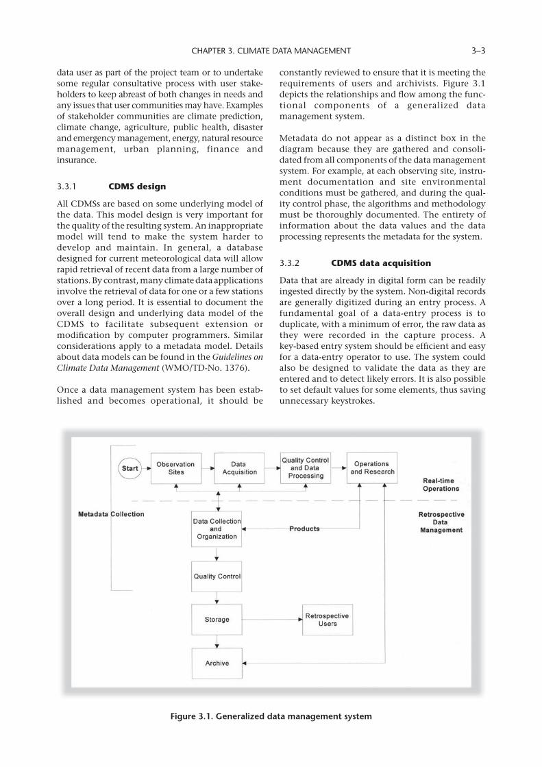
CHAPTER 3. CLIMATE DATA MANAGEMENT 3–3
constantly reviewed to ensure that it is meeting the requirements of users and archivists. Figure 3.1 depicts the relationships and flow among the func-tional components of a generalized data management system.
Metadata do not appear as a distinct box in the diagram because they are gathered and consoli-dated from all components of the data management system. For example, at each observing site, instru-ment documentation and site environmental conditions must be gathered, and during the qual-ity control phase, the algorithms and methodology must be thoroughly documented. The entirety of information about the data values and the data processing represents the metadata for the system.
3.3.2 CDMSdataacquisition
Data that are already in digital form can be readily ingested directly by the system. Non-digital records are generally digitized during an entry process. A fundamental goal of a data-entry process is to duplicate, with a minimum of error, the raw data as they were recorded in the capture process. A key-based entry system should be efficient and easy for a data-entry operator to use. The system could also be designed to validate the data as they are entered and to detect likely errors. It is also possible to set default values for some elements, thus saving unnecessary keystrokes.
data user as part of the project team or to undertake some regular consultative process with user stake-holders to keep abreast of both changes in needs and any issues that user communities may have. Examples of stakeholder communities are climate prediction, climate change, agriculture, public health, disaster and emergency management, energy, natural resource management, urban planning, finance and insurance.
3.3.1 CDMSdesign
All CDMSs are based on some underlying model of the data. This model design is very important for the quality of the resulting system. An inappropriate model will tend to make the system harder to develop and maintain. In general, a database designed for current meteorological data will allow rapid retrieval of recent data from a large number of stations. By contrast, many climate data applications involve the retrieval of data for one or a few stations over a long period. It is essential to document the overall design and underlying data model of the CDMS to facilitate subsequent extension or modification by computer programmers. Similar considerations apply to a metadata model. Details about data models can be found in the Guidelines on Climate Data Management (WMO/TD-No. 1376).
Once a data management system has been estab-lished and becomes operational, it should be
Figure.3 .1 ..Generalized.data.management.system.
GUIDE TO CLIMATOLOGICAL PRACTICES 3–4
Where AWSs are in use, climate data, including any error control messages, should be transferred elec-tronically to the CDMS. Manually observed data should be transferred to the CDMS as soon as possi-ble by whatever means are most practical. It is advantageous to collect data at least daily because data quality is likely to be improved, the manual effort for quality control will likely decrease, tech-nical errors will be detected faster, and there will be greater opportunities for improved access to more data. Nevertheless, the submission of data for a month is an acceptable alternative when daily data transmission is not practicable. For example, many of the 6 000 or so voluntary observers in Australia continue to forward monthly rainfall reports that contain the daily observations for the month.
Many weather observations are recorded by institu-tions or organizations other than NMHSs, and acquisition of the data in their original form may be difficult. In these cases efforts should be made to collect copies of the original report forms. If it is impossible to secure either the original or a copy of the record, a note to this effect should be made in the inventory of the centre’s holdings, stating informa-tion pertaining to the existence and location of the data, volume available, period of record covered, stations in the network as applicable, and elements observed.
Though not a formal requirement, it is recom-mended that the CDMS also contain information about media reports, pictures and other similar information beyond the traditional data and meta-data. Such information could be captured by imaging the report from the print media with a digital camera or scanner; defining the date, area and type of event (such as flood, drought or heavy precipitation); identifying the media; and writing additional comments about the event.
It is important to retain both the data value that was originally received, as well as the latest quality-controlled value. The original value will likely pass through an initial automated quality control proc-ess at ingestion and as necessary, a more extensive quality control process, and even if rejected by either of these processes, it must still be retained. Some CDMSs retain not only the original and latest values, but also all modifications.
Another aspect of data acquisition is the recording of occurrences when data were expected but not received. Loss of data can occur as a result of situa-tions such as inoperable instrumentation, data transmission errors and acquisition processing errors. Lost data can be reconstructed with varying levels of certainty. For example, a missing precipita-tion measurement can be considered to be zero when it is known from other data that local and
synoptic conditions precluded the occurrence of precipitation. In other cases, lost data can be esti-mated with reasonable certainty using the techniques discussed in section 5.9. In all cases, dataset documentation should flag the recon-structed or estimated data appropriately (see 3.4.1).
3.3.3 CDMSdatadocumentation
An adequate set of metadata must be available to inform future users about the nature of the data in the system, how the various datasets were collected, and any inherent problems. It is recommended that database management include all information that can affect the homogeneity of a dataset or series, including those factors outlined in section 2.6.9.
The structure of metadata in an ideal system is generally more complex than the data themselves. For example, a rainfall observation essentially gives the quantity of precipitation over a certain period at a certain station. The associated metadata that can be applied to this observation, and which might be needed to interpret the data fully, could include information such as the reference date used by the database (for example, Greenwich Mean Time (GMT) or time zone); quality indicators or flags that have been ascribed to the observation; history of changes made to the values and any asso-ciated flags; instrument used to record the observation, together with details about mainte-nance programmes, tolerances, internal parameters and similar information; name and contact infor-mation of the observer; full details of the location and siting of a station and its history; programme of observations in effect at the time and its history; and topographical and ground-cover details of the site. A detailed treatment of station-specific meta-data can be found in the Guidelines on Climate Metadata and Homogenization (WMO/TD-No. 1186). As another example, the metadata associated with a gridded dataset of satellite observations of high-resolution solar exposure should include the geographical extent of the observations, the period of record of the dataset, a history of revisions to and maintenance of the dataset, the satellites from which the data were obtained, transfer functions and averaging procedures to obtain grid values, satellite positional accuracy, information about the accuracy of the data, and contact information.
Metadata are also needed for the CDMS itself. Each process within the system (for example, key entry or quality control) should be completely described. A history of any changes made to any part of the system (for example, software, hardware or manual procedures) should be documented and maintained. Since observing practices, quality control techniques and data-handling procedures change over time, these metadata are critical in the climatological
CHAPTER 3. CLIMATE DATA MANAGEMENT 3–5
analysis of historical data. The analyst uses the metadata to identify and understand how a data value was observed and processed in order to separate meteorological from possible non-meteorological influences in the data record.
Another category of metadata is the record of data holdings in the CDMS. Inventories of the data contained in the CDMS should be prepared routinely. Stratification could be, for example, by data element, station location, or time. Lists of contents should be established and maintained to describe and define the data content of the indi-vidual files and to provide information on the codes and observational practices used. Knowing what is contained in the CDMS is important for efficient retrieval of information from the system. The WMO core profile of the ISO 19100 series for data and metadata should be used unless it is superseded by published climate metadata standards.
3.3.4 CDMSdatastorage
An important function of the data manager is to esti-mate data storage requirements, including the estimation of future growth. Account must be taken of the additional information to be included in data records (for example, data quality flags, original messages, and date and time of record updates), metadata needs, and any redundancy necessary to ensure that databases can be restored. Some data types (such as those from remote-sensing, oceanog-raphy and AWSs with high temporal resolution) require large amounts of storage. Unconventional data (such as soil moisture, phenological observa-tions and vegetation indices) may have storage needs that are different from the more traditional observa-tions. AWSs will often generate data that are relevant to the quality of observations, but are not strictly climate data (for example, information on the battery-level voltage for an AWS). Generally, this information should be utilized prior to data archiv-ing; if it is not included in the CDMS, it should be permanently retained elsewhere and made accessi-ble to data managers. The quality control process often generates values and information that may be different from the original data, so there is a storage requirement for keeping both the original data and any different data generated by quality control proc-esses. Estimating future growth can be very difficult, as it is hard to determine what data types may become available as time and technology progress. The data manager must consider all of these factors when determining storage requirements.
Non-digital records should be stored in a way that minimizes their deterioration. They should be stored in a controlled environment to avoid temperature and humidity extremes, insects, pests, fire, flood, acci-dents or deliberate destruction. An ideal example
would be storage in acid-free boxes in air-conditioned, secure storerooms. A maintenance programme should be established to rescue deteriorating documents and particularly the data they contain.
With an ever-increasing amount of information being generated and retained, the problem arises as to whether or not to continue to store all the records in their original manuscript form. All too often, climatological records are stored in basements, sheds and other undesirable facilities. They are frequently not catalogued, and they may be inac-cessible and subject to deterioration. As a means of reducing paper costs, making better use of space, and providing security for original documents, it is recommended that the manuscript data be scanned into a digital file and carefully preserved. The elec-tronic images of the paper records can then be stored and retrieved using computer technologies such as optical character recognition software. The specifications of computer hardware required for storing and retrieving documents depend on data needs and the limits of financial resources, and also on technological advances, so there are no global standards or a preferred single storage medium. It is important to remember that no storage medium is permanent, and therefore regular review of archival arrangements should be undertaken. Computer-based archives must be securely and regularly backed up with at least one copy stored at a site separate from the main archive.
Microform refers to document images photographi-cally reduced to a very small fraction of their original size. A variety of microform formats exist. Examples are microfilm reels, microfiche sheets, jackets, film folios, aperture cards, cartridges and cassettes. Significant advances in digital storage capabilities, however, now make it highly desirable that paper documents be directly scanned or digit-ally photographed into a computer system along with superseded microform images. This process facilitates access and ensures preservation for future generations.
3.3.5 CDMSdataaccessandretrieval
An important aspect of any CDMS is the power of the facilities to perform data retrieval and analysis. Graphical user interface retrieval facilities should be provided for most users, and command line facilities should be available for the small number of knowledgeable users who have a need for non-standard retrievals. Users should be able to specify their own retrieval criteria, and the system docu-mentation should be clear and provide as much information as necessary to support the users.
Output options should be extensive and include facilities for customizing stations, times and details
GUIDE TO CLIMATOLOGICAL PRACTICES 3–6
of output presentations. Access should be given to listings of data, tabular summaries, statistical analy-ses and graphical presentation.
3.3.6 CDMSarchives
An archive is the permanent retention of the data and metadata in the CDMS. The archive structure, whether simple or complex, physical or electronic, should be guided by financial resources, the degree of training of archive personnel, the volume of data to be archived, the media of the data (such as paper documents or digital format), the ease of putting information into and retrieving information from the archive, user-friendliness in accessing information, the ease of maintenance of the archive, and the ease of expan-sion as data holdings increase. All aspects of the CDMS should be archived, including not just the data values but also catalogues, inventories, histories, dictionaries, and other similar information.
3.3.7 CDMSsecurity
The main goal of a security policy and associated activities is to prevent loss of or damage to the CDMS. To satisfy this goal, the requisites are:(a) All personnel must be aware of their profes-
sional responsibilities;(b) The archives and database environment must be
secured and protected against physical hazards to the records, such as fire and excess humidity;
(c) For digital data, user-level security should be enforced with respect to the database and its components. Only a small and registered group of people should have the right to perform data manipulations such as inser-tions, updates or deletions;
(d) Personnel with write access to a database must agree not to perform any transactions besides the operations and practices approved by the data manager;
(e) All changes to data tables should have an audit trail, and controls on access to this trail should be in place;
(f) Password security principles should be applied, including not sharing passwords, not writing passwords on paper, changing pass-words regularly, and using “strong” passwords consisting of seemingly unrelated letters, numbers and characters;
(g) All unnecessary services should be disabled on the database computer;
(h) The database must be protected against attacks from viruses and hackers;
(i) Regular backups must be made, noting that work done after the most recent backup will likely be lost and need to be repeated should a computer failure occur. Typically, an incre-mental backup should be made daily and a full backup weekly;
(j) Every so often, typically monthly, a complete backup of the data tables should be put in a safe, secure, fireproof location, remote from the physical location of the climate database. It is common to have three copies of the same archive in differ-ent secure places and if possible in different towns or cities;
(k) Backups of the CDMS must be performed prior to any changes to the system software, to the system design or to the applications contained in the CDMS.
3.3.8 CDMSmanagement
A CDMS should be monitored routinely to deter-mine how well the processes using and supporting the database are performing. Examples of the proc-esses that support the data are metadata maintenance, database ingest, quality control actions that modify the database, and information retrieval. Each process should be monitored, evaluated, and if necessary, improved. It is strongly recommended that data managers think in terms of end-to-end data manage-ment, with information on systemic data quality issues, loss of data, or other practices that harm the climate record being referred back to observation managers for rectification.
Typical monitoring reports would include the number and type of stations in the database, the quantity of data in the database grouped by stations and by observation element types, and information about missing data. This information can be compared to observation schedules to identify when and where data are being lost. Other reports could include quality control actions to ensure that the quality control process is performing properly with new data or to identify any groupings of data with excessive quality problems. It is useful to track the quantity and range of data being retrieved for user inquiries, since this information is helpful in indicating both the most important datasets and the areas to be developed in the future.
The frequency and reporting period of monitoring reports depend on the needs of the NMHS. Reports on data ingestion may be made automatically, perhaps every day. Monthly reports on the quantity and quality of data usually match the monthly cycle of many climate products.
3.3.9 InternationalCDMSstandardsandguidelines
There is no agreement on the optimal structure of a climatological database, as the design depends on the specific needs of the NMHSs and stakeholders. One need may be to access all data for a specified element over a region for a given time, but another
CHAPTER 3. CLIMATE DATA MANAGEMENT 3–7
need may be to access a data time series for the same element for a single location. The particular needs will have a strong impact on the required storage space or the response time to load or to access data. General principles that should be followed in any design, however, include:(a) User documentation: Manuals should include
an overview and guides for installation, users, system administrators and programmers;
(b) Key entry: On-screen layouts of data input forms should be similar to the layout of the paper forms from which the data are being copied, customizing of layouts should be possible, procedures for making entries into the database should meet the needs of the NMHS, validation of entries (for example, permissible values or station identifiers) should be automatically performed in the key entry process, and default values should be entered automatically;
(c) Ingest of digital data: The system should be able to automatically ingest standard format-ted data that are transmitted via the Global Telecommunication System (GTS), files containing data for multiple stations, multiple files containing data for a single station, data from AWSs, data with user-defined formats, CLICOM data, and metadata;
(d) Validation and quality control: The system should provide flags indicating the data source, level of quality assurance performed (such as key entry process or end-of-month processing), quality assurance results, and the reason for the decision to accept, reject or estimate a value. It should retain original, estimated and changed data values; it should also evaluate data temporally and spatially for permissible values, meteorological consist-ency and physical reasonableness;
(e) Technical documentation: There must be listings defining each table in the database and the relationships among tables; naming conventions should be consistent among all tables, indexes, entities and views;
(f) Data access: The interface between the user and the database should be easy to use, and procedures for extracting information should be documented with clear instructions and examples;
(g) Metadata: The system must be able to manage the full range of metadata (as described in section 2.6.9);
(h) Output products: CDMSs should be able to produce standard output products that meet the needs of the NMHS, such as data listings and tabulations of hourly, daily, monthly and longer-period data; statistical summaries; and graphical depictions such as contour analyses, windroses, time series, upper-air soundings and station model plots;
(i) Data and system administration: The system should be capable of being backed up routinely and on demand without being shut down; of being restored as needed in a timely manner; of logging individual transactions; of maintaining security; of being monitored for system performance (for example, memory usage, available storage space, number of transactions and status of system logs); and of being copied at regular intervals to a separate physical location;
(j) Level of assistance: Users should be able to solve problems using available documenta-tion, interact with other users to exchange questions and comments, and obtain advice from developers of the system as needed and in a timely manner;
(k) Flexibility: The system should be capable of being expanded and modified as hardware and software technologies evolve and data sources change, and as the need for output products changes.
3.4 QUALITYCONTROL
The objective of quality control is to verify whether a reported data value is representative of what was intended to be measured and has not been contam-inated by unrelated factors. It is important therefore to be clear from the outset what the readings of a particular data series are meant to represent. Data should be considered as satisfactory for permanent archiving only after they have been subjected to adequate quality control.
The observer or automated observing system should apply quality control to ensure that the time and station identification are correct, that the recorded values reliably reflect current conditions, and that there is consistency among the observed elements. These steps must all be taken prior to the recording or transmission of an observation.
The archiving centre should also apply quality control to the observations received. If manuscript records constitute the source document, trained personnel should, upon receipt at the archiving centre, scrutinize them before any digitization takes place. The forms should be reviewed to ensure proper identification (for example, station name, identifying number and location), legibility, and proper recording of data (for example, to the correct precision and in the proper columns). If any problems are discovered, the observation sites should be contacted to clarify the issues or correct the problems. If resources do not permit the quality control of all data, priority should be given to the most important climate elements.
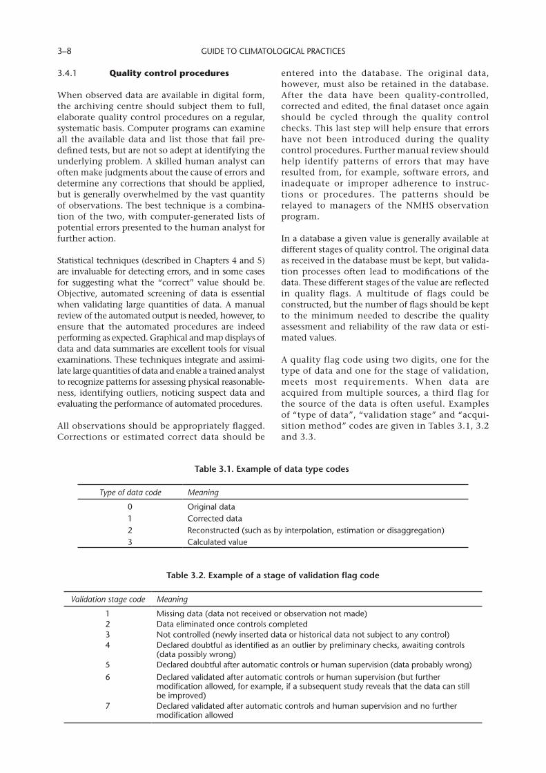
GUIDE TO CLIMATOLOGICAL PRACTICES 3–8
Type of data code Meaning
0 Original data1 Corrected data2 Reconstructed (such as by interpolation, estimation or disaggregation)3 Calculated value
Table.3 .2 ..Example.of.a.stage.of.validation.flag.code..
Validation stage code Meaning
1 Missing data (data not received or observation not made)2 Data eliminated once controls completed3 Not controlled (newly inserted data or historical data not subject to any control)4 Declared doubtful as identified as an outlier by preliminary checks, awaiting controls
(data possibly wrong)5 Declared doubtful after automatic controls or human supervision (data probably wrong)6 Declared validated after automatic controls or human supervision (but further
modification allowed, for example, if a subsequent study reveals that the data can still be improved)
7 Declared validated after automatic controls and human supervision and no further modification allowed
3.4.1 Qualitycontrolprocedures
When observed data are available in digital form, the archiving centre should subject them to full, elaborate quality control procedures on a regular, systematic basis. Computer programs can examine all the available data and list those that fail pre-defined tests, but are not so adept at identifying the underlying problem. A skilled human analyst can often make judgments about the cause of errors and determine any corrections that should be applied, but is generally overwhelmed by the vast quantity of observations. The best technique is a combina-tion of the two, with computer-generated lists of potential errors presented to the human analyst for further action.
Statistical techniques (described in Chapters 4 and 5) are invaluable for detecting errors, and in some cases for suggesting what the “correct” value should be. Objective, automated screening of data is essential when validating large quantities of data. A manual review of the automated output is needed, however, to ensure that the automated procedures are indeed performing as expected. Graphical and map displays of data and data summaries are excellent tools for visual examinations. These techniques integrate and assimi-late large quantities of data and enable a trained analyst to recognize patterns for assessing physical reasonable-ness, identifying outliers, noticing suspect data and evaluating the performance of automated procedures.
All observations should be appropriately flagged. Corrections or estimated correct data should be
entered into the database. The original data, however, must also be retained in the database. After the data have been quality-controlled, corrected and edited, the final dataset once again should be cycled through the quality control checks. This last step will help ensure that errors have not been introduced during the quality control procedures. Further manual review should help identify patterns of errors that may have resulted from, for example, software errors, and inadequate or improper adherence to instruc-tions or procedures. The patterns should be relayed to managers of the NMHS observation program.
In a database a given value is generally available at different stages of quality control. The original data as received in the database must be kept, but valida-tion processes often lead to modifications of the data. These different stages of the value are reflected in quality flags. A multitude of flags could be constructed, but the number of flags should be kept to the minimum needed to describe the quality assessment and reliability of the raw data or esti-mated values.
A quality flag code using two digits, one for the type of data and one for the stage of validation, meets most requirements. When data are acquired from multiple sources, a third flag for the source of the data is often useful. Examples of “type of data”, “validation stage” and “acqui-sition method” codes are given in Tables 3.1, 3.2 and 3.3.
Table.3 .1 ..Example.of.data.type.codes
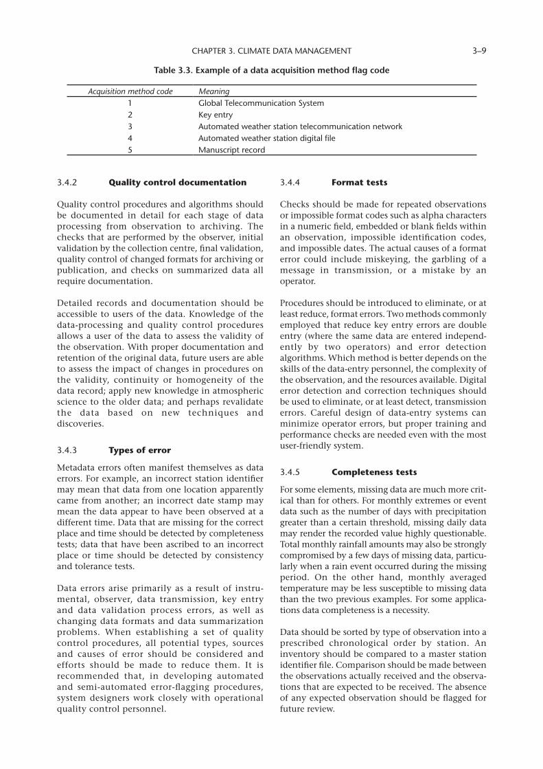
CHAPTER 3. CLIMATE DATA MANAGEMENT 3–9
3.4.2 Qualitycontroldocumentation
Quality control procedures and algorithms should be documented in detail for each stage of data processing from observation to archiving. The checks that are performed by the observer, initial validation by the collection centre, final validation, quality control of changed formats for archiving or publication, and checks on summarized data all require documentation.
Detailed records and documentation should be accessible to users of the data. Knowledge of the data-processing and quality control procedures allows a user of the data to assess the validity of the observation. With proper documentation and retention of the original data, future users are able to assess the impact of changes in procedures on the validity, continuity or homogeneity of the data record; apply new knowledge in atmospheric science to the older data; and perhaps revalidate the data based on new techniques and discoveries.
3.4.3 Typesoferror
Metadata errors often manifest themselves as data errors. For example, an incorrect station identifier may mean that data from one location apparently came from another; an incorrect date stamp may mean the data appear to have been observed at a different time. Data that are missing for the correct place and time should be detected by completeness tests; data that have been ascribed to an incorrect place or time should be detected by consistency and tolerance tests.
Data errors arise primarily as a result of instru-mental, observer, data transmission, key entry and data validation process errors, as well as changing data formats and data summarization problems. When establishing a set of quality control procedures, all potential types, sources and causes of error should be considered and efforts should be made to reduce them. It is recommended that, in developing automated and semi-automated error-flagging procedures, system designers work closely with operational quality control personnel.
3.4.4 Formattests
Checks should be made for repeated observations or impossible format codes such as alpha characters in a numeric field, embedded or blank fields within an observation, impossible identification codes, and impossible dates. The actual causes of a format error could include miskeying, the garbling of a message in transmission, or a mistake by an operator.
Procedures should be introduced to eliminate, or at least reduce, format errors. Two methods commonly employed that reduce key entry errors are double entry (where the same data are entered independ-ently by two operators) and error detection algorithms. Which method is better depends on the skills of the data-entry personnel, the complexity of the observation, and the resources available. Digital error detection and correction techniques should be used to eliminate, or at least detect, transmission errors. Careful design of data-entry systems can minimize operator errors, but proper training and performance checks are needed even with the most user-friendly system.
3.4.5 Completenesstests
For some elements, missing data are much more crit-ical than for others. For monthly extremes or event data such as the number of days with precipitation greater than a certain threshold, missing daily data may render the recorded value highly questionable. Total monthly rainfall amounts may also be strongly compromised by a few days of missing data, particu-larly when a rain event occurred during the missing period. On the other hand, monthly averaged temperature may be less susceptible to missing data than the two previous examples. For some applica-tions data completeness is a necessity.
Data should be sorted by type of observation into a prescribed chronological order by station. An inventory should be compared to a master station identifier file. Comparison should be made between the observations actually received and the observa-tions that are expected to be received. The absence of any expected observation should be flagged for future review.
Table.3 .3 ..Example.of.a.data.acquisition.method.flag.code
Acquisition method code Meaning1 Global Telecommunication System2 Key entry3 Automated weather station telecommunication network4 Automated weather station digital file5 Manuscript record

GUIDE TO CLIMATOLOGICAL PRACTICES 3–10
3.4.6 Consistencytests
The four primary types of consistency checks are internal, temporal, spatial and summarization. Since data values are interrelated in time and space, an integrated procedure should be developed to examine consistency. All consistency tests should be completely documented with procedures, formu-lae and decision criteria.
Internal consistency relies on the physical relation-ships among climatological elements. All elements should be thoroughly verified against any associ-ated elements within each observation. For example, psychrometric data should be checked to ensure that the reported dry bulb temperature equals or exceeds the reported wet bulb tempera-ture. Similarly, the relationship between visibility and present weather should be checked for adher-ence to standard observation practices.
Data should be checked for consistency with defi-nitions. For example, a maximum value must be equal to or higher than a minimum value. Physical bounds provide rules for further internal consist-ency checks. For example, sunshine duration is limited by the duration of the day, global radia-tion cannot be greater than the irradiance at the top of the atmosphere, wind direction must be between 0° and 360°, and precipitation cannot be negative.
Temporal consistency tests the variation of an element in time. Many climatological datasets show significant serial correlation. A check should be made by comparing the prior and subsequent observations with the one in question. Using expe-rience or analytical or statistical methodologies, data reviewers can establish the amount of change that might be expected in a particular element in any time interval. This change usually depends on the element, season, location and time lag between two successive observations. For example, a temper-ature drop of 10°C within one hour may be suspect, but could be quite realistic if associated with the passage of a cold front or onset of a sea breeze. The suspicious value will have to be compared to present weather at that time, and perhaps to other types of observations (such as wind direction or satellite, radar or lightning detection) before a decision is made to validate or modify it. For some elements, a lack of change could indicate an error. For example, a series of identical wind speeds may indicate a problem with the anemometer.
Temporal consistency checks can be automated easily. Section 5.5 describes some of the techniques of time series analysis, which can be adapted for quality control purposes. Graphical displays of data are also excellent tools for verification. Several
elements should be visualized at the same time in order to facilitate diagnostics. For example, it will be easier to validate a temperature drop if the infor-mation showing the veering of winds associated with the passage of a cold front, or heavy rain from a thunderstorm, is also available.
Spatial consistency compares each observation with observations taken at the same time at other stations in the area. Each observation can be compared to what would be expected at that site based on the observations from neighbouring stations. Those data for which there is a significant difference between the expected and actual obser-vations should be flagged for review, correction or deletion as necessary. It is important to recognize that only like quantities should be directly compared, such as wind speeds measured at the same height; values measured at similar eleva-tions, such as flat, open topography; or values measured within a climatologically similar area. Section 5.9 details the data estimation techniques that are required for this type of quality control process.
Summarization tests are among the easiest to perform. By comparing different summaries of data, errors in individual values or in each summary can be detected. For example, the sums and means of daily values can be calculated for various periods such as weeks, months or years. Checking that the total of the twelve monthly reported sums equals the sum of the individual daily values for a year provides a quick and simple cross-check for an accumulation element like rain-fall. Systematic errors in upper-air station data can sometimes be revealed by comparing monthly averages with the averages derived for the same location and height from a numerical analysis system. The cause of any inconsistencies should be reviewed and corrected.
Marine observations, in general, can be subjected to procedures similar to those used for surface land stations, with slight modification for addi-tional elements, assuming that there is a ship identifier present in each observation to allow data to be sorted chronologically and by ship order. Upper-air observations must be verified in a somewhat different manner. Some cross-checks should be made on surface-level conditions with those at a nearby or co-located surface station. A quality control programme to check upper-air data should compute successive level data from the preceding level starting with the surface data. Limits on the difference allowed between the computed and reported values should be estab-lished. Any level with reported elements that fail the test should be flagged as suspect, reviewed or corrected.
CHAPTER 3. CLIMATE DATA MANAGEMENT 3–11
resolutions address the concepts of “essential” and “additional” data, with a specification of a minimum set of data that should be made available in a non-discriminatory manner and at a charge of no more than the cost of reproduction and delivery, without requiring payment for the data and products them-selves. Members may decide to declare as “essential” more than the minimum set. The use of agreed-upon international standard formats for data exchange is critical.
Beyond CLIMAT and related messages (see section 4.8.7), Members are also asked to provide additional data and products that are needed to sustain WMO programmes at the global, regional and national levels and to assist other Members in providing meteorological and climatological services in their countries. Members supplying such additional data and products may place conditions on their re-export. Research and educational communities should be provided with free and unrestricted access to all data and products exchanged under the auspices of WMO for their non-commercial activities.
Members of WMO voluntarily nominate subsets of their stations to be parts of various networks, including the Global Climate Observing System (GCOS) Upper-Air Network (GUAN), the GCOS Surface Network (GSN), the Regional Basic Synoptic Network and the Regional Basic Climatological Network. Nomination of stations to participate in these networks implies an obligation to share the data internationally.
Data are also shared through International Council for Science (ICSU) World Data Centres (WDCs). The WDC system works to guarantee access to solar, geophysical and related environmental data. It serves the whole scientific community by assem-bling, scrutinizing, organizing and disseminating data and information. The centres collect, docu-ment and archive measurements and the associated metadata from stations worldwide and make these data freely available to the scientific community. In some cases, WDCs also provide additional prod-ucts, including data analyses, maps of data distributions, and data summaries. There are climate-related ICSU World Data Centres covering meteorology, paleoclimatology, oceanography, atmospheric trace gases, glaciology, soils, marine geology and geophysics, sunspots, solar activity, solar–terrestrial physics, airglow, aurora, and cosmic rays, as well as other disciplines.
The World Meteorological Organization is actively involved in the provision of data to a number of these WDCs, and there are a number of associated centres operated directly through WMO. The WMO centres deal with ozone and ultraviolet radiation, greenhouse
3.4.7 Tolerancetests
Tolerance tests set upper or lower limits on the possible values of a climatological element (such as wind direction, cloud cover, and past and present weather), or in other cases where the theoretical range of values is infinite, the limits outside of which it is unlikely for a measurement to lie. In the latter case, the limits are usually time- and location-dependent and should be established by recourse to the historical values or by spatial interpolation methods. It is also important to identify and then quickly address systematic biases in the outputs from instrumentation. Documentation must be maintained regarding which tolerance tests have been applied, the climate limits established for each inspected element, and the rationale for determin-ing these limits.
In general, tolerance tests compare a value in ques-tion against some standard using a statistical threshold. Some simple tolerance tests include comparing an observed value to the extreme or record value or to some multiple of standard devia-tions around the average value for that date. In the latter case, one must take into consideration the possibility that the element may not necessarily have a symmetrical or Gaussian distribution, and that some extreme values identified from the stand-ard deviation multiplier may be incorrect.
When using long-term historical data for quality control, it is preferable to use a standardized refer-ence (for example, standard deviations or a non-parametric rank order statistic) rather than an absolute reference. Section 4.4 discusses the various summary descriptors of data, including the restric-tions on their appropriateness.
It may be possible to perform some tolerance tests using completely different data streams, such as satellite or radar data. For example, a very simple test for the occurrence or non-occurrence of precip-itation using satellite data would be to check for the presence of clouds in a satellite image.
3.5 EXCHANGEOFCLIMATICDATA
Exchange of data is essential for climatology. For WMO Members, the obligation to share data and metadata with other Members, and the conditions under which these may be passed to third parties, are covered under Resolution 40 of the Twelfth World Meteorological Congress (with regard to meteoro-logical data), Resolution 25 of the Thirteenth World Meteorological Congress (for hydrological data), and Intergovernmental Oceanographic Commission Resolution XXII-6 (for oceanographic data). These
GUIDE TO CLIMATOLOGICAL PRACTICES 3–12
International data exchange agreements allow for the global compilation of publications such as Climatic Normals, World Weather Records, and Monthly Climatic Data for the World. Bilateral or multilateral agreements are also important in creat-ing and exchanging long-term datasets, such as the Global Historical Climate Network, Comprehensive Aerological Reference, and Comprehensive Ocean–Atmosphere Data Sets compiled by the United States, and the Hadley Centre global observations datasets compiled by the United Kingdom. These datasets are generally provided to research centres.
The current WMO information systems have been developed to meet a diverse set of needs for many different programmes and commissions. The multi-plicity of systems has resulted in incompatibilities, inefficiencies, duplication of effort and higher over-all costs for Members. An alternative approach planned to improve efficiency of the transfer of data and information among countries is the WMO Information System (WIS). It is envisioned that this system will be used for the collection and sharing of information for all WMO and related international programmes. Non-meteorological and non-climatic environmental and geophysical data such as ecologi-cal, earthquake and tsunami data could be included. The WIS vision provides guidance for the orderly evolution of existing systems into an integrated system that efficiently meets the international envi-ronmental information requirements of Members.
The WMO Information System will provide an inte-grated approach to routine collection and automated dissemination of observed data and products, timely delivery of data and products, and requests for data and products. It should be reliable, cost-effective and affordable for developing as well as developed Members. It should also be technologically sustaina-ble and appropriate to local expertise, modular, scalable, flexible and extensible. It should be able to adjust to changing requirements, allow dissemination of products from diverse data sources, and allow participants to collaborate at levels appropriate to their responsibilities and budgetary resources. The WMO Information System should also support differ-ent user groups and access policies such as those outlined in Resolutions 40 and 25 referred to above, data as well as network security, and integration of diverse datasets.
3.6 DATARESCUE
Data rescue is recognized now as a two-part process, as defined in the Report of the CLICOM-DARE Workshop (WMO/TD-No. 1128). First there is the ongoing process of preserving all data at risk of being lost due to deterioration of the medium, and
gases, aerosols, aerosol optical depth, radiation and precipitation chemistry. There are differences in data access policy for ICSU and WMO centres. International Council for Science data centres exchange data among themselves without charge and provide data to scien-tists in any country free of charge. Data centres operated through WMO must abide by Resolutions 40 and 25 referred to above, which allow for some data or products to be placed in the WDCs with conditions attached to their use.
In addition to the International Council for Science WDCs, there are many other centres that operate under cooperative agreements with WMO or with individual NMHSs. These centres include the Global Precipitation Climatology Centre and Global Runoff Data Centre (Germany); Australia’s National Climate Centre; the World Ozone and Ultraviolet Radiation Data Centre (Canada); the Met Office Hadley Centre (United Kingdom of Great Britain and Northern Ireland); and in the United States of America, the Lamont-Doherty Earth Observatory of Columbia University, the National Climatic Data Center, the National Oceanographic Data Center, the National Geophysical Data Center, the National Aeronautics and Space Administration (NASA) Goddard Distributed Active Archive Center, the Tropical Pacific Ocean Observing Array, and the University Corporation for Atmospheric Research.
Exchange of digital data is simple for many Members because of the range of computer commu-nications systems available. The Global Telecommunication System is a meteorological communication system with connections to virtu-ally all countries of the world. As an operational system with a critical role in global weather fore-casting, it provides reliable communication services, albeit sometimes with low bandwidth. Like the Internet, the Global Telecommunication System is based on a confederation of interconnected networks. As a closed system, however, it is free from the security breaches that often plague the Internet. Open communication linkages such as the Internet should be protected by the best avail-able security software systems to minimize the danger of unwanted access and file manipulation or corruption.
It is highly unlikely that archived formats used for climatological data by one country would be the same as those used by another. The format docu-mentation describing the data organization, element types, units and any other pertinent infor-mation should accompany the data. In addition, if the digital data are compacted or in a special non-text format, it is extremely useful for the contributing archive centre to provide “read” routines to accompany digital data requested from an archive.
CHAPTER 3. CLIMATE DATA MANAGEMENT 3–13
then there is the digitization of data into computer-compatible form for easy access. Each NMHS should establish and maintain a data rescue programme.
In the mid-1990s technological advancements made it possible to optically scan climate data as a new method of creating digital climate archives. This technology permits the data not only to be preserved, but also to be in a form suitable for exchange via computer media. Optically scanning images preserves the data and is a major improve-ment over hard-copy media, but these data should be moved into digital databases for use in analyses and product development (see section 3.3.4). To ensure that digital files will always be accessible: (a) Data should be stored as image files on media
such as cartridges, CDs and DVDs that can be regularly renewed to prevent loss from deterioration of the medium;
(b) Data should be digitized and entered into a CDMS;
(c) Data already in computer-compatible media should be migrated as soon as possible to storage facilities that conform to new and accepted technologies;
(d) Data formats should also be migrated to formats that conform to software changes.
3.7 REFERENCES
3.7.1 WMOpublications
World Meteorological Organization, 1988: WMO Region III/IV Training Seminar on Climate Data Management and User Service (Barbados, 22–26 September 1986; Panama, 29 September–3 October 1986) (WMO/TD-No. 227, WCDP-No. 1), Geneva.
———, 1989: CLICOM Project (Climate Data Management System) (WMO/TD-No. 299, WCDP-No. 6), Geneva.
———, 1989: Report of the Meeting of CLICOM Experts (Paris, 11–15 September 1989) (WMO/TD- No. 342, WCDP-No. 9), Geneva.
———, 1990: Report of the Expert Group on Global Baseline Datasets (Asheville, North Carolina, 22–26 January 1990) (WMO/TD-No. 359, WCDP-No. 11), Geneva.
———, 1990: Report of the Meeting on Archival Survey for Climate History (Paris, 21–22 February 1990) (WMO/TD-No. 372, WCDP-No. 12), Geneva.
———, 1992: CCl Working Group on Climate Data (Geneva, 11–15 November 1991) (WMO/TD- No. 488, WCDMP-No. 18), Geneva.
———, 1992: Report of the First Session of the Advisory Committee on Climate Applications and Data (ACCAD) (Geneva, 19–20 November 1991) (WMO/TD-No. 475, WCASP-No. 18, WCDMP- No. 17), Geneva.
———, 1993. Advisory Committee on Climate Applications and Data (ACCAD) (Report of the second session, Geneva, 16–17 November 1992) (WMO/TD-No. 529, WCASP-No. 22, WCDMP- No. 22), Geneva.
———, 1993: Final Report of the CCl Working Group on Climate Data and its Rapporteurs to the Eleventh Session of the Commission for Climatology (Havana, 15–26 February 1993) (WMO/TD- No. 523, WCDMP-No. 21), Geneva.
———, 1996: Report of the Fifth Session of the Advisory Committee on Climate Applications and Data (ACCAD) (Geneva, 26 September 1995) (WMO/TD-No. 712, WCASP-No. 35, WCDMP-No. 25), Geneva.
———, 1996: Report on the Status of the Archival Climate History Survey (ARCHISS) Project (WMO/TD-No. 776, WCDMP-No. 26), Geneva.
———, 1997: Expert Meeting to Review and Assess the Oracle-Based Prototype for Future Climate Database Management Systems (CDMS) (Toulouse, 12–16 May 1997) (WMO/TD-No. 902, WCDMP-No. 34), Geneva.
———, 1997: Meeting of the CCl Working Group on Climate Data: Summary Report, (Geneva, 30 January–3 February 1995) (WMO/TD- No. 841, WCDMP-No. 33), Geneva.
———, 1997: Reports for CCl-XII from Rapporteurs that Relate to Climate Data Management (WMO/TD- No. 833, WCDMP-No. 31), Geneva.
———, 1997: Summary Notes and Recommendations Assembled for CCl-XII from Recent Activities Concerning Climate Data Management (WMO/TD- No. 832, WCDMP-No. 30), Geneva.
———, 1999: Report of the Meeting of the WMO Commission for Climatology Task Group on a Future WMO Climate Database Management System (Ostrava, Czech Republic, 10–13 November 1998) and Follow-up Workshop to the WMO CCl Task Group Meeting on a Future WMO CDMS (Toulouse, 30 March–1 April 1999) (WMO/TD-No. 932, WCDMP-No. 38), Geneva.
———, 1999: Proceedings of the Second Seminar for Homogenization of Surface Climatological Data (Budapest, Hungary, 9–13 November 1998) (WMO/TD-No. 962, WCDMP-No. 41), Geneva.
———, 1999: Meeting of the CCl Working Group on Climate Data (Geneva, 30 November–4 December 1998) (WMO/TD-No. 970, WCDMP-No. 39), Geneva.
———, 1999: Report of the Training Seminar on Climate Data Management Focusing on CLICOM/CLIPS Development and Evaluation (Niamey, Niger, 3 May–10 July 1999) (WMO/TD-No. 973, WCDMP-No. 43), Geneva.
———, 2000: CLICOM 3.1. Release 2. Geneva.———, 2000: GCOS/GOOS/GTOS Joint Data and
Information Management Plan, 2000 (WMO/TD- No. 1004, GCOS-No. 60), Geneva.
GUIDE TO CLIMATOLOGICAL PRACTICES 3–14
———, 2000: Representativeness, Data Gaps and Uncertainties in Climate Observations, Invited Scientific Lecture given by Chris Folland to the Thirteenth World Meteorological Congress (Geneva, 21 May 1999) (WMO/TD-No. 977, WCDMP-No. 44), Geneva.
———, 2000: Task Group on Future WMO Climate Database Management Systems (Geneva, 3–5 May 2000) (WMO/TD-No. 1025, WCDMP-No. 46), Geneva.
———, 2002: Guide to the GCOS Surface and Upper-Air Networks. GSN and GUAN, Version 1.1 (WMO/TD-No. 1106, GCOS-No. 73), Geneva.
———, 2002: Report of the CLICOM-DARE Workshop (San José, Costa Rica, 17–28 July 2002); Report of the International Data Rescue Meeting (Geneva, 11–13 September 2001) (WMO/TD-No. 1128, WCDMP-No. 49), Geneva.
———, 2002: Report of the Climate Database Management Systems Evaluation Workshop (Geneva, 27 May–1 June 2002) (WMO/TD- No. 1130, WCDMP-No. 50), Geneva.
———, 2003: Guidelines on Climate Metadata and Homogenization (WMO/TD-No. 1186, WCDMP- No. 53), Geneva.
———, 2004: Guidelines on Climate Data Rescue (WMO/TD-No. 1210, WCDMP-No. 55), Geneva.
———, 2004: Fourth Seminar for Homogenization and Quality Control in Climatological Databases (Budapest, 6–10 October 2003) (WMO/TD- No. 1236, WCDMP-No. 56), Geneva.
———, 2007: Guidelines on Climate Data Management (WMO/TD-No. 1376, WCDMP-No. 56), Geneva.
3.7.2 Additionalreading
Cornford, D., 1998: An overview of interpolation. In: Seminar on Data Spatial Distribution in Meteorology and Climatology (M. Bindi and B. Gozzini, eds). Volterra, European Union COST Action 79.
De Gaetano, A.T., 1997: A quality control proce-dure for hourly wind data. J. Atmos. Oceanic Technol., 14:137–151.
Graybeal, D.Y., A.T. De Gaetano and K.L. Eggleston, 2004: Complex quality assurance of historical hourly surface airways meteorological data. J. Atmos. Oceanic Technol., 21:1156–1169.
Hungarian Meteorological Service, 1997: Proceedings of the First Seminar for Homogenization of Surface Climatological Data (Budapest, 6–12 October 1996), Budapest.
Kresse, W. and K. Fadaie, 2004: ISO Standards for Geographic Information. Berlin, Springer.
Merlier, C., 2001: Interpolation des Données Spatiales en Climatologie, et Conception Optimale des Réseaux Climatologiques. Annexe du rapport de Météo-France concernant ses activités en rapport avec la Commission for Climatology (CCl) de l’OMM. WMO report, CCl Lead Rapporteur on Statistical Methods with Emphasis on Spatial Interpolation.
.
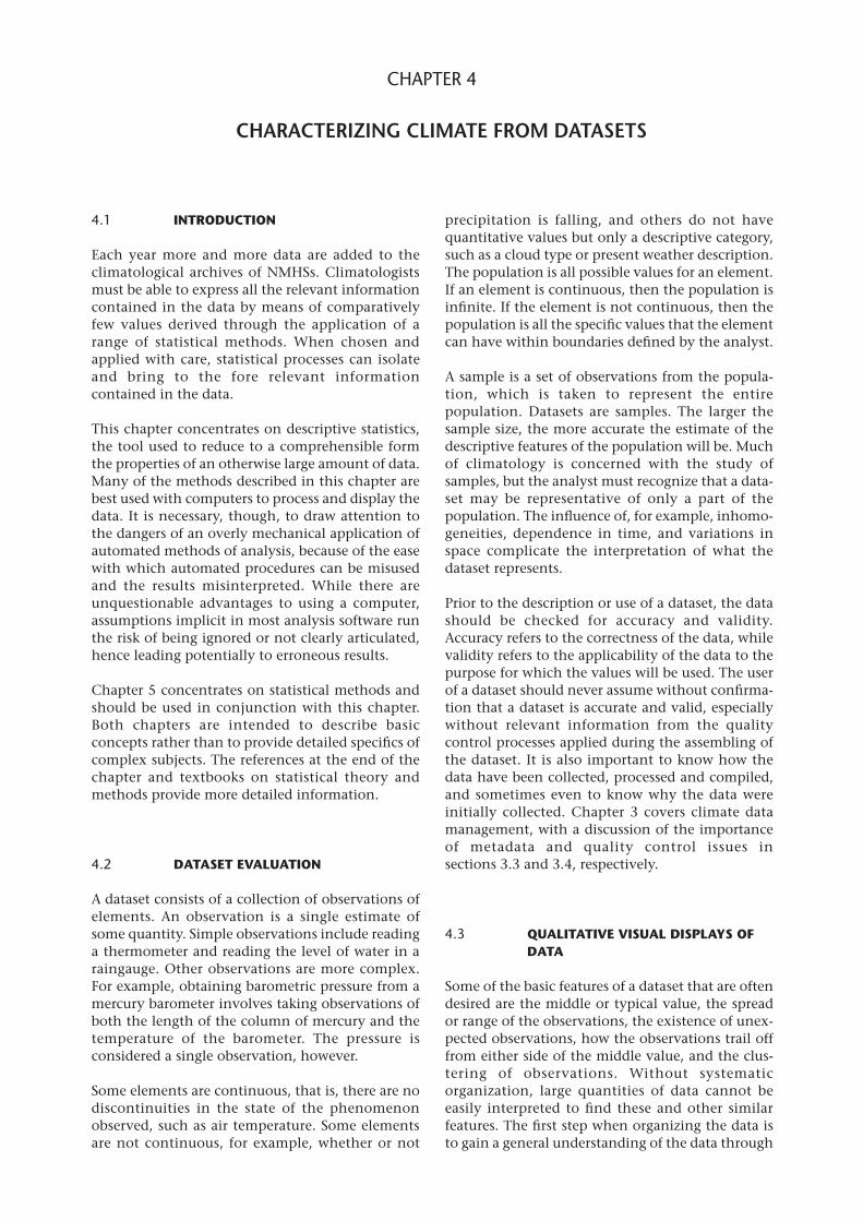
����CHARACTERIZING.CLIMATE.FROM.DATASETS
CHAPTER 4
4.1 INTRODUCTION
Each year more and more data are added to the climatological archives of NMHSs. Climatologists must be able to express all the relevant information contained in the data by means of comparatively few values derived through the application of a range of statistical methods. When chosen and applied with care, statistical processes can isolate and bring to the fore relevant information contained in the data.
This chapter concentrates on descriptive statistics, the tool used to reduce to a comprehensible form the properties of an otherwise large amount of data. Many of the methods described in this chapter are best used with computers to process and display the data. It is necessary, though, to draw attention to the dangers of an overly mechanical application of automated methods of analysis, because of the ease with which automated procedures can be misused and the results misinterpreted. While there are unquestionable advantages to using a computer, assumptions implicit in most analysis software run the risk of being ignored or not clearly articulated, hence leading potentially to erroneous results.
Chapter 5 concentrates on statistical methods and should be used in conjunction with this chapter. Both chapters are intended to describe basic concepts rather than to provide detailed specifics of complex subjects. The references at the end of the chapter and textbooks on statistical theory and methods provide more detailed information.
4.2 DATASETEVALUATION
A dataset consists of a collection of observations of elements. An observation is a single estimate of some quantity. Simple observations include reading a thermometer and reading the level of water in a raingauge. Other observations are more complex. For example, obtaining barometric pressure from a mercury barometer involves taking observations of both the length of the column of mercury and the temperature of the barometer. The pressure is considered a single observation, however.
Some elements are continuous, that is, there are no discontinuities in the state of the phenomenon observed, such as air temperature. Some elements are not continuous, for example, whether or not
precipitation is falling, and others do not have quantitative values but only a descriptive category, such as a cloud type or present weather description. The population is all possible values for an element. If an element is continuous, then the population is infinite. If the element is not continuous, then the population is all the specific values that the element can have within boundaries defined by the analyst.
A sample is a set of observations from the popula-tion, which is taken to represent the entire population. Datasets are samples. The larger the sample size, the more accurate the estimate of the descriptive features of the population will be. Much of climatology is concerned with the study of samples, but the analyst must recognize that a data-set may be representative of only a part of the population. The influence of, for example, inhomo-geneities, dependence in time, and variations in space complicate the interpretation of what the dataset represents.
Prior to the description or use of a dataset, the data should be checked for accuracy and validity. Accuracy refers to the correctness of the data, while validity refers to the applicability of the data to the purpose for which the values will be used. The user of a dataset should never assume without confirma-tion that a dataset is accurate and valid, especially without relevant information from the quality control processes applied during the assembling of the dataset. It is also important to know how the data have been collected, processed and compiled, and sometimes even to know why the data were initially collected. Chapter 3 covers climate data management, with a discussion of the importance of metadata and quality control issues in sections 3.3 and 3.4, respectively.
4.3 QUALITATIVEVISUALDISPLAYSOFDATA
Some of the basic features of a dataset that are often desired are the middle or typical value, the spread or range of the observations, the existence of unex-pected observations, how the observations trail off from either side of the middle value, and the clus-tering of observations. Without systematic organization, large quantities of data cannot be easily interpreted to find these and other similar features. The first step when organizing the data is to gain a general understanding of the data through
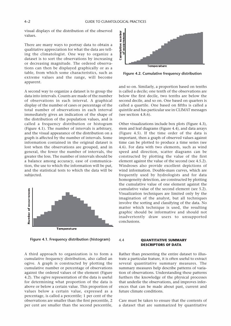
GUIDE TO CLIMATOLOGICAL PRACTICES 4–2
visual displays of the distribution of the observed values.
There are many ways to portray data to obtain a qualitative appreciation for what the data are tell-ing the climatologist. One way to organize a dataset is to sort the observations by increasing or decreasing magnitude. The ordered observa-tions can then be displayed graphically or as a table, from which some characteristics, such as extreme values and the range, will become apparent.
A second way to organize a dataset is to group the data into intervals. Counts are made of the number of observations in each interval. A graphical display of the number of cases or percentage of the total number of observations in each interval immediately gives an indication of the shape of the distribution of the population values, and is called a frequency distribution or histogram (Figure 4.1). The number of intervals is arbitrary, and the visual appearance of the distribution on a graph is affected by the number of intervals. Some information contained in the original dataset is lost when the observations are grouped, and in general, the fewer the number of intervals, the greater the loss. The number of intervals should be a balance among accuracy, ease of communica-tion, the use to which the information will be put, and the statistical tests to which the data will be subjected.
A third approach to organization is to form a cumulative frequency distribution, also called an ogive. A graph is constructed by plotting the cumulative number or percentage of observations against the ordered values of the element (Figure 4.2). The ogive representation of the data is useful for determining what proportion of the data is above or below a certain value. This proportion of values below a certain value, expressed as a percentage, is called a percentile; 1 per cent of the observations are smaller than the first percentile, 2 per cent are smaller than the second percentile,
and so on. Similarly, a proportion based on tenths is called a decile; one tenth of the observations are below the first decile, two tenths are below the second decile, and so on. One based on quarters is called a quartile. One based on fifths is called a quintile and has particular use in CLIMAT messages (see section 4.8.6).
Other visualizations include box plots (Figure 4.3), stem and leaf diagrams (Figure 4.4), and data arrays (Figure 4.5). If the time order of the data is important, then a graph of observed values against time can be plotted to produce a time series (see 4.6). For data with two elements, such as wind speed and direction, scatter diagrams can be constructed by plotting the value of the first element against the value of the second (see 4.5.2). Windroses also provide excellent depictions of wind information. Double-mass curves, which are frequently used by hydrologists and for data homogeneity detection, are constructed by plotting the cumulative value of one element against the cumulative value of the second element (see 5.2). Visualization techniques are limited only by the imagination of the analyst, but all techniques involve the sorting and classifying of the data. No matter which technique is used, the resulting graphic should be informative and should not inadvertently draw users to unsupported conclusions.
4.4 QUANTITATIVESUMMARYDESCRIPTORSOFDATA
Rather than presenting the entire dataset to illus-trate a particular feature, it is often useful to extract several quantitative summary measures. The summary measures help describe patterns of varia-tion of observations. Understanding these patterns furthers the knowledge of the physical processes that underlie the observations, and improves infer-ences that can be made about past, current and future climate conditions.
Care must be taken to ensure that the contents of a dataset that are summarized by quantitative
Figure.4 .1 ..Frequency.distribution.(histogram)
Figure.4 .2 ..Cumulative.frequency.distribution
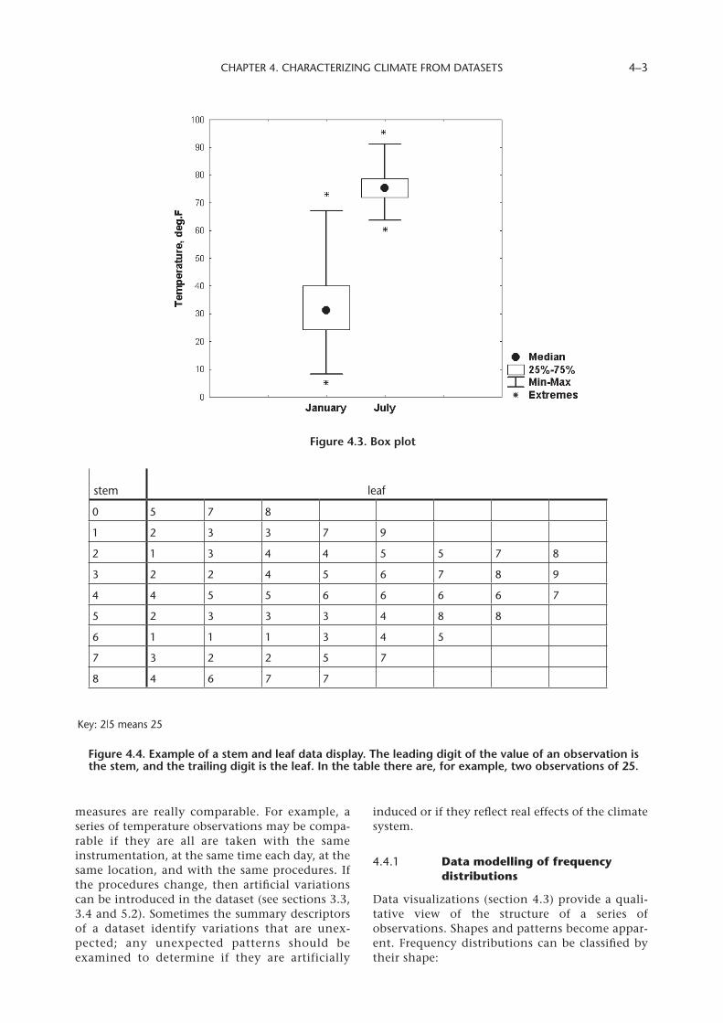
CHAPTER 4. CHARACTERIZING CLIMATE FROM DATASETS 4–3
induced or if they reflect real effects of the climate system.
4.4.1 Datamodellingoffrequencydistributions
Data visualizations (section 4.3) provide a quali-tative view of the structure of a series of observations. Shapes and patterns become appar-ent. Frequency distributions can be classified by their shape:
measures are really comparable. For example, a series of temperature observations may be compa-rable if they are all are taken with the same instrumentation, at the same time each day, at the same location, and with the same procedures. If the procedures change, then artificial variations can be introduced in the dataset (see sections 3.3, 3.4 and 5.2). Sometimes the summary descriptors of a dataset identify variations that are unex-pected; any unexpected patterns should be examined to determine if they are artificially
Figure.4 .3 ..Box.plot
Figure.4 .4 ..Example.of.a.stem.and.leaf.data.display ..The.leading.digit.of.the.value.of.an.observation.is.the.stem,.and.the.trailing.digit.is.the.leaf ..In.the.table.there.are,.for.example,.two.observations.of.25 .
stem leaf
0 5 7 8
1 2 3 3 7 9
2 1 3 4 4 5 5 7 8
3 2 2 4 5 6 7 8 9
4 4 5 5 6 6 6 6 7
5 2 3 3 3 4 8 8
6 1 1 1 3 4 5
7 3 2 2 5 7
8 4 6 7 7
Key: 2|5 means 25
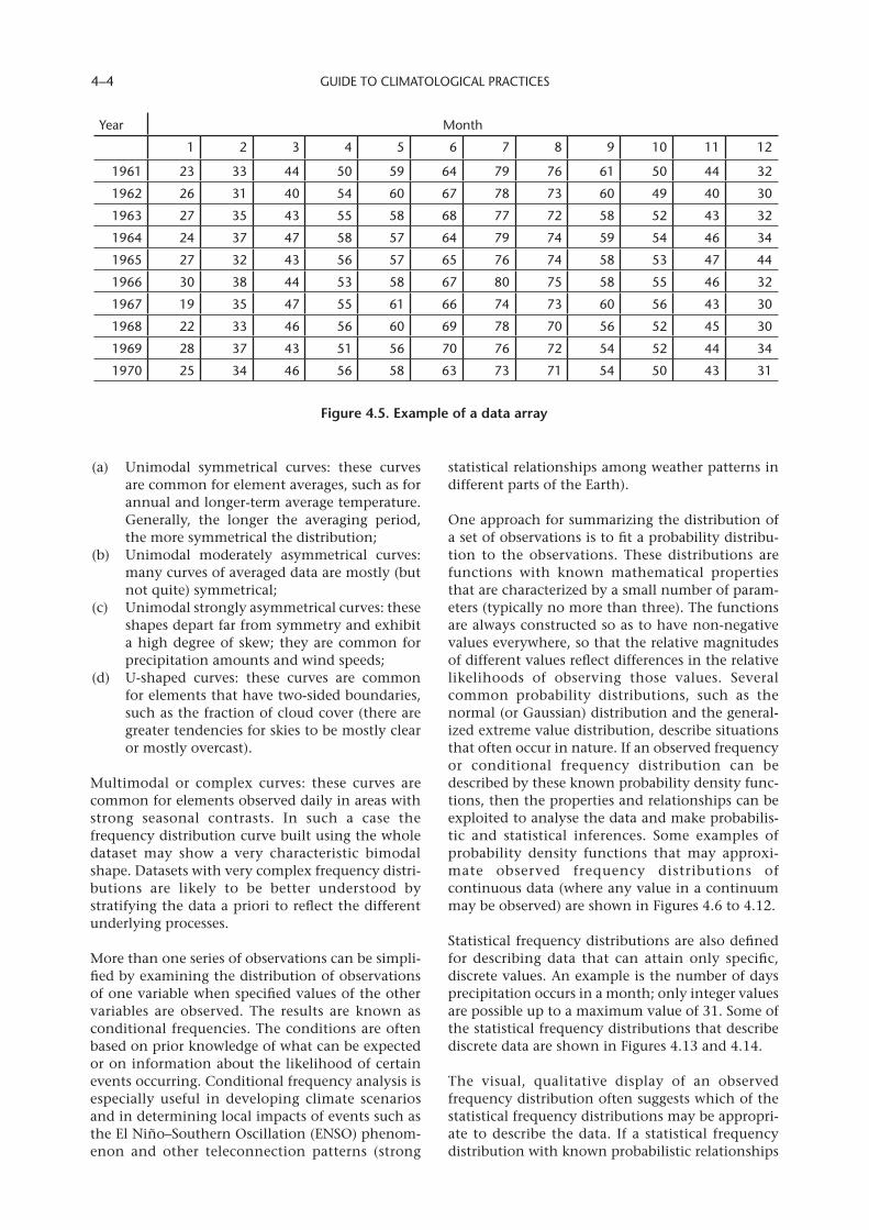
GUIDE TO CLIMATOLOGICAL PRACTICES 4–4
(a) Unimodal symmetrical curves: these curves are common for element averages, such as for annual and longer-term average temperature. Generally, the longer the averaging period, the more symmetrical the distribution;
(b) Unimodal moderately asymmetrical curves: many curves of averaged data are mostly (but not quite) symmetrical;
(c) Unimodal strongly asymmetrical curves: these shapes depart far from symmetry and exhibit a high degree of skew; they are common for precipitation amounts and wind speeds;
(d) U-shaped curves: these curves are common for elements that have two-sided boundaries, such as the fraction of cloud cover (there are greater tendencies for skies to be mostly clear or mostly overcast).
Multimodal or complex curves: these curves are common for elements observed daily in areas with strong seasonal contrasts. In such a case the frequency distribution curve built using the whole dataset may show a very characteristic bimodal shape. Datasets with very complex frequency distri-butions are likely to be better understood by stratifying the data a priori to reflect the different underlying processes.
More than one series of observations can be simpli-fied by examining the distribution of observations of one variable when specified values of the other variables are observed. The results are known as conditional frequencies. The conditions are often based on prior knowledge of what can be expected or on information about the likelihood of certain events occurring. Conditional frequency analysis is especially useful in developing climate scenarios and in determining local impacts of events such as the El Niño–Southern Oscillation (ENSO) phenom-enon and other teleconnection patterns (strong
statistical relationships among weather patterns in different parts of the Earth).
One approach for summarizing the distribution of a set of observations is to fit a probability distribu-tion to the observations. These distributions are functions with known mathematical properties that are characterized by a small number of param-eters (typically no more than three). The functions are always constructed so as to have non-negative values everywhere, so that the relative magnitudes of different values reflect differences in the relative likelihoods of observing those values. Several common probability distributions, such as the normal (or Gaussian) distribution and the general-ized extreme value distribution, describe situations that often occur in nature. If an observed frequency or conditional frequency distribution can be described by these known probability density func-tions, then the properties and relationships can be exploited to analyse the data and make probabilis-tic and statistical inferences. Some examples of probability density functions that may approxi-mate observed frequency distributions of continuous data (where any value in a continuum may be observed) are shown in Figures 4.6 to 4.12.
Statistical frequency distributions are also defined for describing data that can attain only specific, discrete values. An example is the number of days precipitation occurs in a month; only integer values are possible up to a maximum value of 31. Some of the statistical frequency distributions that describe discrete data are shown in Figures 4.13 and 4.14.
The visual, qualitative display of an observed frequency distribution often suggests which of the statistical frequency distributions may be appropri-ate to describe the data. If a statistical frequency distribution with known probabilistic relationships
Figure.4 .5 ..Example.of.a.data.array
Year Month
1 2 3 4 5 6 7 8 9 10 11 12
1961 23 33 44 50 59 64 79 76 61 50 44 32
1962 26 31 40 54 60 67 78 73 60 49 40 30
1963 27 35 43 55 58 68 77 72 58 52 43 32
1964 24 37 47 58 57 64 79 74 59 54 46 34
1965 27 32 43 56 57 65 76 74 58 53 47 44
1966 30 38 44 53 58 67 80 75 58 55 46 32
1967 19 35 47 55 61 66 74 73 60 56 43 30
1968 22 33 46 56 60 69 78 70 56 52 45 30
1969 28 37 43 51 56 70 76 72 54 52 44 34
1970 25 34 46 56 58 63 73 71 54 50 43 31
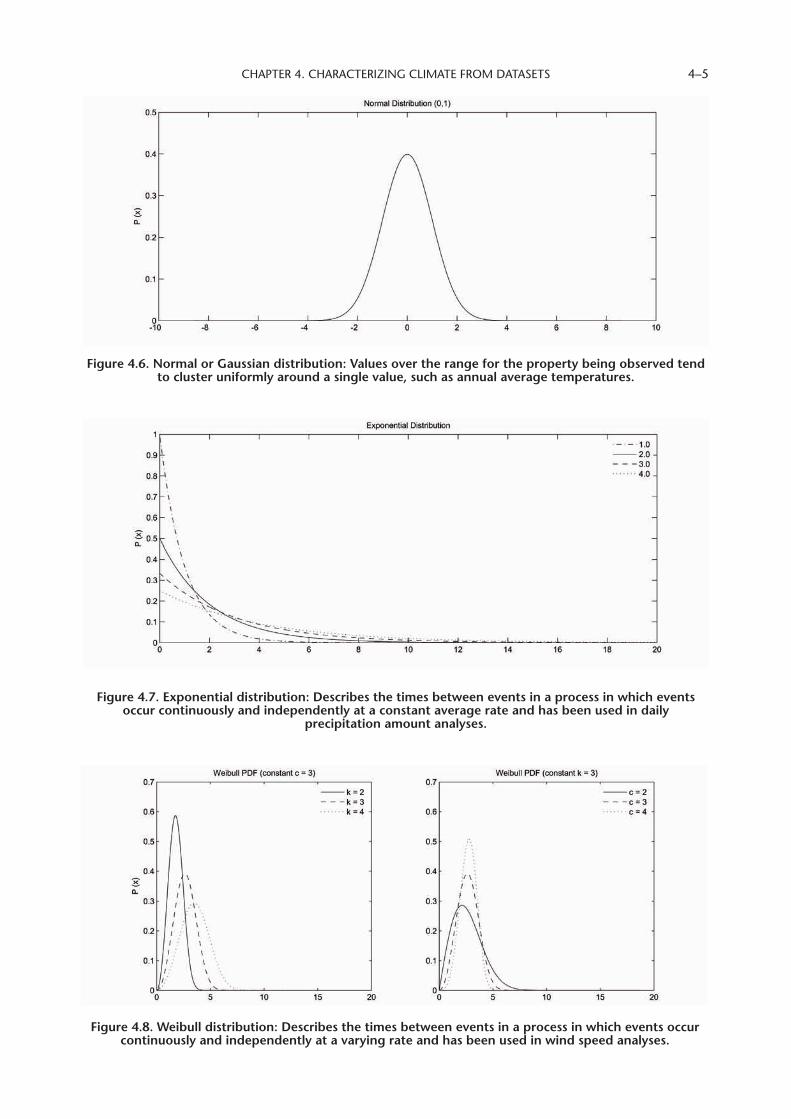
CHAPTER 4. CHARACTERIZING CLIMATE FROM DATASETS 4–5
Figure.4 .6 ..Normal.or.Gaussian.distribution:.Values.over.the.range.for.the.property.being.observed.tend.to.cluster.uniformly.around.a.single.value,.such.as.annual.average.temperatures .
Figure.4 .7 ..Exponential.distribution:.Describes.the.times.between.events.in.a.process.in.which.events.occur.continuously.and.independently.at.a.constant.average.rate.and.has.been.used.in.daily..
precipitation.amount.analyses .
Figure.4 .8 ..Weibull.distribution:.Describes.the.times.between.events.in.a.process.in.which.events.occur.continuously.and.independently.at.a.varying.rate.and.has.been.used.in.wind.speed.analyses .
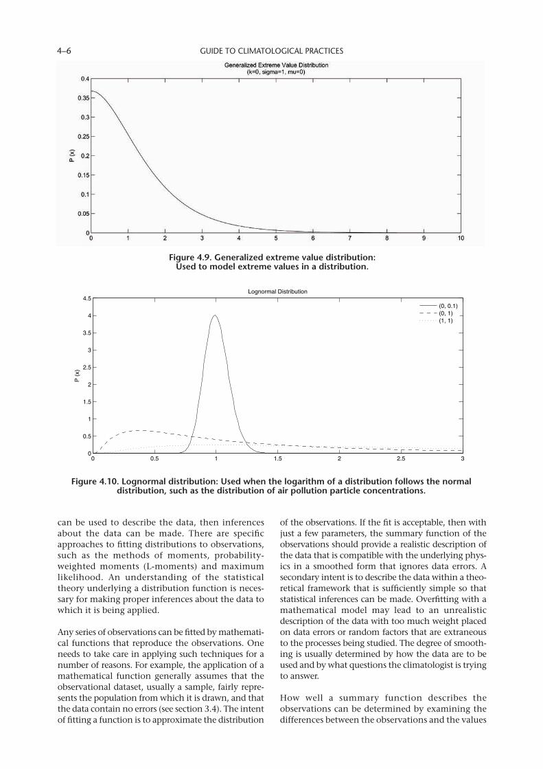
GUIDE TO CLIMATOLOGICAL PRACTICES 4–6
can be used to describe the data, then inferences about the data can be made. There are specific approaches to fitting distributions to observations, such as the methods of moments, probability-weighted moments (L-moments) and maximum likelihood. An understanding of the statistical theory underlying a distribution function is neces-sary for making proper inferences about the data to which it is being applied.
Any series of observations can be fitted by mathemati-cal functions that reproduce the observations. One needs to take care in applying such techniques for a number of reasons. For example, the application of a mathematical function generally assumes that the observational dataset, usually a sample, fairly repre-sents the population from which it is drawn, and that the data contain no errors (see section 3.4). The intent of fitting a function is to approximate the distribution
of the observations. If the fit is acceptable, then with just a few parameters, the summary function of the observations should provide a realistic description of the data that is compatible with the underlying phys-ics in a smoothed form that ignores data errors. A secondary intent is to describe the data within a theo-retical framework that is sufficiently simple so that statistical inferences can be made. Overfitting with a mathematical model may lead to an unrealistic description of the data with too much weight placed on data errors or random factors that are extraneous to the processes being studied. The degree of smooth-ing is usually determined by how the data are to be used and by what questions the climatologist is trying to answer.
How well a summary function describes the observations can be determined by examining the differences between the observations and the values
Figure.4 .9 ..Generalized.extreme.value.distribution:..Used.to.model.extreme.values.in.a.distribution .
0 0.5 1 1.5 2 2.5 30
0.5
1
1.5
2
2.5
3
3.5
4
4.5
P (x
)
Lognormal Distribution
(0, 0.1)(0, 1)(1, 1)
Figure.4 .10 ..Lognormal.distribution:.Used.when.the.logarithm.of.a.distribution.follows.the.normal.distribution,.such.as.the.distribution.of.air.pollution.particle.concentrations .
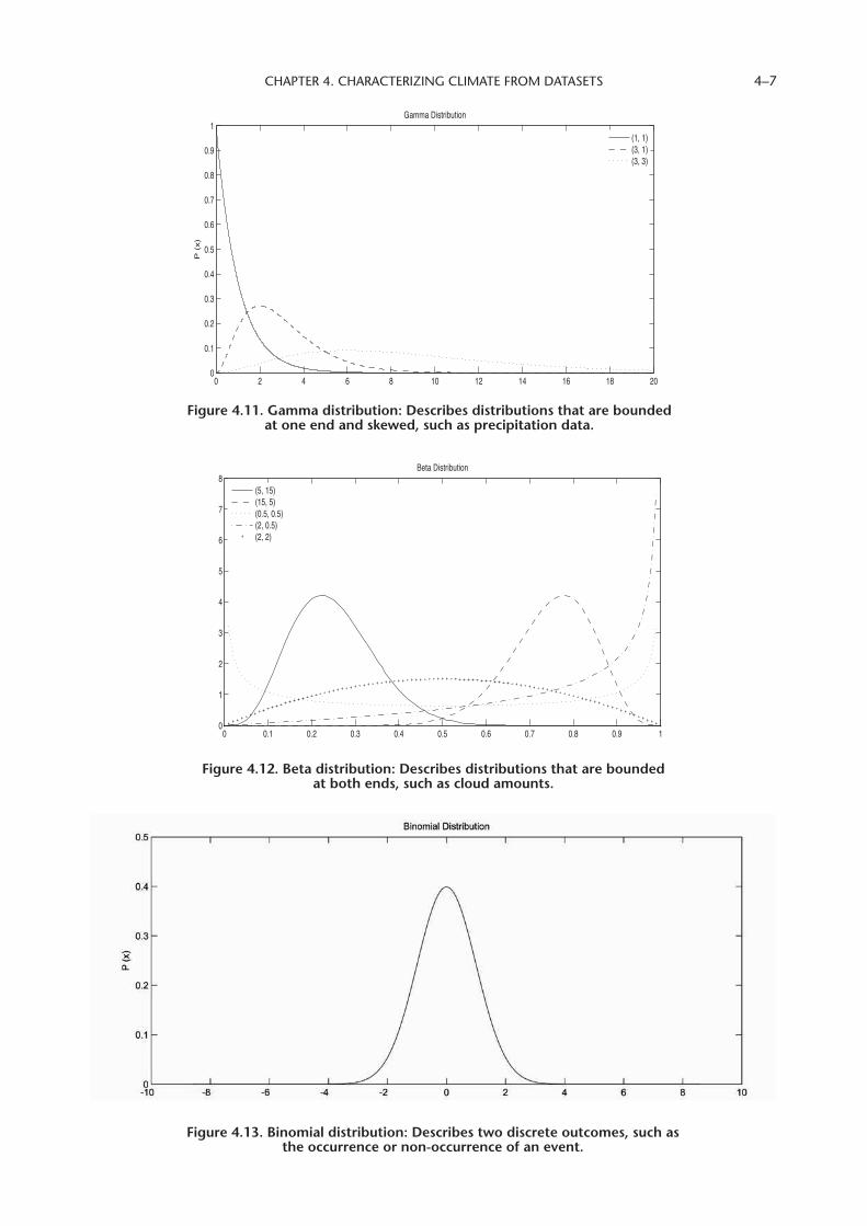
CHAPTER 4. CHARACTERIZING CLIMATE FROM DATASETS 4–7
Figure.4 .11 ..Gamma.distribution:.Describes.distributions.that.are.bounded..at.one.end.and.skewed,.such.as.precipitation.data .
Figure.4 .12 ..Beta.distribution:.Describes.distributions.that.are.bounded..at.both.ends,.such.as.cloud.amounts .
0 2 4 6 8 10 12 14 16 18 200
0.1
0.2
0.3
0.4
0.5
0.6
0.7
0.8
0.9
1
P (
x)
Gamma Distribution
(1, 1)(3, 1)(3, 3)
0 0.1 0.2 0.3 0.4 0.5 0.6 0.7 0.8 0.9 10
1
2
3
4
5
6
7
8Beta Distribution
(5, 15)(15, 5)(0.5, 0.5)(2, 0.5)(2, 2)
Figure.4 .13 ..Binomial.distribution:.Describes.two.discrete.outcomes,.such.as..the.occurrence.or.non-occurrence.of.an.event .
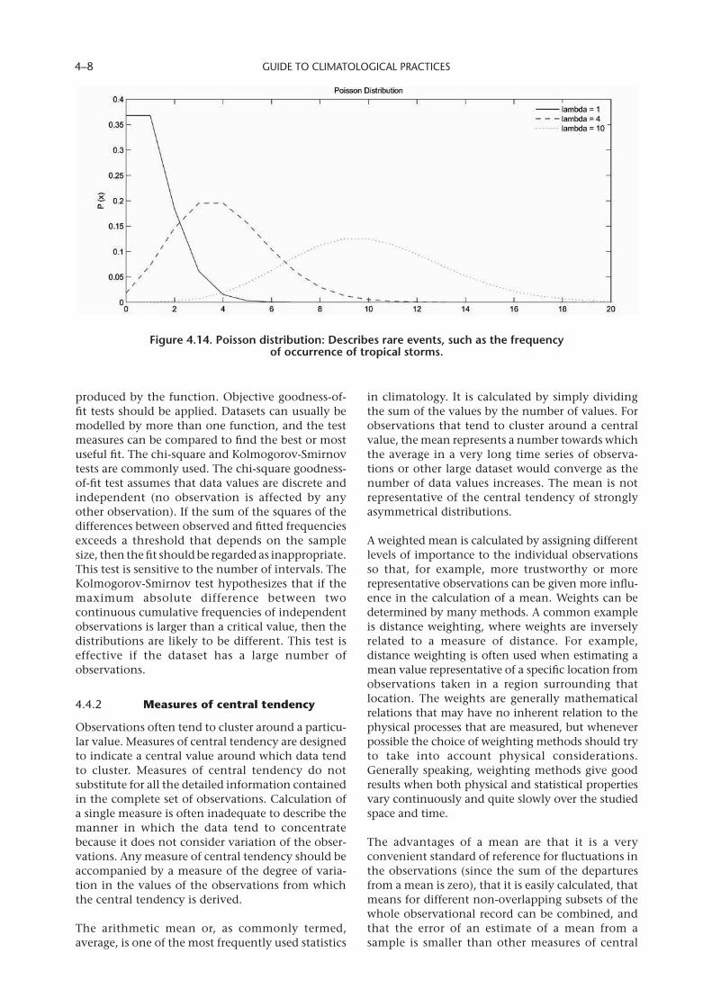
GUIDE TO CLIMATOLOGICAL PRACTICES 4–8
produced by the function. Objective goodness-of-fit tests should be applied. Datasets can usually be modelled by more than one function, and the test measures can be compared to find the best or most useful fit. The chi-square and Kolmogorov-Smirnov tests are commonly used. The chi-square goodness-of-fit test assumes that data values are discrete and independent (no observation is affected by any other observation). If the sum of the squares of the differences between observed and fitted frequencies exceeds a threshold that depends on the sample size, then the fit should be regarded as inappropriate. This test is sensitive to the number of intervals. The Kolmogorov-Smirnov test hypothesizes that if the maximum absolute difference between two continuous cumulative frequencies of independent observations is larger than a critical value, then the distributions are likely to be different. This test is effective if the dataset has a large number of observations.
4.4.2 Measuresofcentraltendency
Observations often tend to cluster around a particu-lar value. Measures of central tendency are designed to indicate a central value around which data tend to cluster. Measures of central tendency do not substitute for all the detailed information contained in the complete set of observations. Calculation of a single measure is often inadequate to describe the manner in which the data tend to concentrate because it does not consider variation of the obser-vations. Any measure of central tendency should be accompanied by a measure of the degree of varia-tion in the values of the observations from which the central tendency is derived.
The arithmetic mean or, as commonly termed, average, is one of the most frequently used statistics
in climatology. It is calculated by simply dividing the sum of the values by the number of values. For observations that tend to cluster around a central value, the mean represents a number towards which the average in a very long time series of observa-tions or other large dataset would converge as the number of data values increases. The mean is not representative of the central tendency of strongly asymmetrical distributions.
A weighted mean is calculated by assigning different levels of importance to the individual observations so that, for example, more trustworthy or more representative observations can be given more influ-ence in the calculation of a mean. Weights can be determined by many methods. A common example is distance weighting, where weights are inversely related to a measure of distance. For example, distance weighting is often used when estimating a mean value representative of a specific location from observations taken in a region surrounding that location. The weights are generally mathematical relations that may have no inherent relation to the physical processes that are measured, but whenever possible the choice of weighting methods should try to take into account physical considerations. Generally speaking, weighting methods give good results when both physical and statistical properties vary continuously and quite slowly over the studied space and time.
The advantages of a mean are that it is a very convenient standard of reference for fluctuations in the observations (since the sum of the departures from a mean is zero), that it is easily calculated, that means for different non-overlapping subsets of the whole observational record can be combined, and that the error of an estimate of a mean from a sample is smaller than other measures of central
Figure.4 .14 ..Poisson.distribution:.Describes.rare.events,.such.as.the.frequency.of.occurrence.of.tropical.storms .
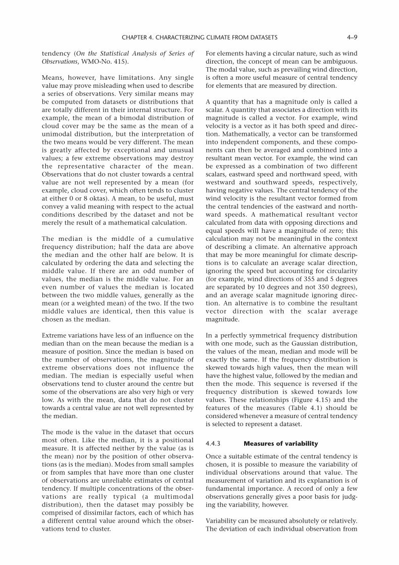
CHAPTER 4. CHARACTERIZING CLIMATE FROM DATASETS 4–9
tendency (On the Statistical Analysis of Series of Observations, WMO-No. 415).
Means, however, have limitations. Any single value may prove misleading when used to describe a series of observations. Very similar means may be computed from datasets or distributions that are totally different in their internal structure. For example, the mean of a bimodal distribution of cloud cover may be the same as the mean of a unimodal distribution, but the interpretation of the two means would be very different. The mean is greatly affected by exceptional and unusual values; a few extreme observations may destroy the representative character of the mean. Observations that do not cluster towards a central value are not well represented by a mean (for example, cloud cover, which often tends to cluster at either 0 or 8 oktas). A mean, to be useful, must convey a valid meaning with respect to the actual conditions described by the dataset and not be merely the result of a mathematical calculation.
The median is the middle of a cumulative frequency distribution; half the data are above the median and the other half are below. It is calculated by ordering the data and selecting the middle value. If there are an odd number of values, the median is the middle value. For an even number of values the median is located between the two middle values, generally as the mean (or a weighted mean) of the two. If the two middle values are identical, then this value is chosen as the median.
Extreme variations have less of an influence on the median than on the mean because the median is a measure of position. Since the median is based on the number of observations, the magnitude of extreme observations does not influence the median. The median is especially useful when observations tend to cluster around the centre but some of the observations are also very high or very low. As with the mean, data that do not cluster towards a central value are not well represented by the median.
The mode is the value in the dataset that occurs most often. Like the median, it is a positional measure. It is affected neither by the value (as is the mean) nor by the position of other observa-tions (as is the median). Modes from small samples or from samples that have more than one cluster of observations are unreliable estimates of central tendency. If multiple concentrations of the obser-vations are really typical (a multimodal distribution), then the dataset may possibly be comprised of dissimilar factors, each of which has a different central value around which the obser-vations tend to cluster.
For elements having a circular nature, such as wind direction, the concept of mean can be ambiguous. The modal value, such as prevailing wind direction, is often a more useful measure of central tendency for elements that are measured by direction.
A quantity that has a magnitude only is called a scalar. A quantity that associates a direction with its magnitude is called a vector. For example, wind velocity is a vector as it has both speed and direc-tion. Mathematically, a vector can be transformed into independent components, and these compo-nents can then be averaged and combined into a resultant mean vector. For example, the wind can be expressed as a combination of two different scalars, eastward speed and northward speed, with westward and southward speeds, respectively, having negative values. The central tendency of the wind velocity is the resultant vector formed from the central tendencies of the eastward and north-ward speeds. A mathematical resultant vector calculated from data with opposing directions and equal speeds will have a magnitude of zero; this calculation may not be meaningful in the context of describing a climate. An alternative approach that may be more meaningful for climate descrip-tions is to calculate an average scalar direction, ignoring the speed but accounting for circularity (for example, wind directions of 355 and 5 degrees are separated by 10 degrees and not 350 degrees), and an average scalar magnitude ignoring direc-tion. An alternative is to combine the resultant vector direction with the scalar average magnitude.
In a perfectly symmetrical frequency distribution with one mode, such as the Gaussian distribution, the values of the mean, median and mode will be exactly the same. If the frequency distribution is skewed towards high values, then the mean will have the highest value, followed by the median and then the mode. This sequence is reversed if the frequency distribution is skewed towards low values. These relationships (Figure 4.15) and the features of the measures (Table 4.1) should be considered whenever a measure of central tendency is selected to represent a dataset.
4.4.3 Measuresofvariability
Once a suitable estimate of the central tendency is chosen, it is possible to measure the variability of individual observations around that value. The measurement of variation and its explanation is of fundamental importance. A record of only a few observations generally gives a poor basis for judg-ing the variability, however.
Variability can be measured absolutely or relatively. The deviation of each individual observation from
GUIDE TO CLIMATOLOGICAL PRACTICES 4–10
the central tendency can be reduced to a value that represents and describes the entire dataset. This single number is the absolute variability.
The simplest measure of absolute variability is the range of the observations. The range is the difference between the highest and lowest values. Although easy to calculate, the range has many limitations. If the extreme values are very rare or they fall well beyond the bulk of observations, then the range will
be misleading. The range imparts no information about the nature of the frequency distribution within the extreme limits. The range also ignores the degree of concentration of the values almost entirely, and fails to characterize in a useful manner the data-set as a whole. Also, the range offers no basis for judging the reliability of the central tendency.
The interquartile range is another common meas-ure of absolute variability. It is the difference
Figure.4 .15 ..Relationships.among.the.mean,.median.and.mode
Feature Mean Median Mode
Affected by outliers Yes No No
Representative of central tendency when frequency distributions are narrowly spread
Yes Yes Yes
Representative of central tendency when frequency distributions are widely spread
No Maybe No
Representative of central tendency when observations are clustered into more than one group
No Maybe No
Representative of central tendency when frequency distributions with one cluster are skewed
No Yes Yes
Ease of calculation Easiest Easy from ordered data
Easy from histogram
Departures sum to zero Yes Not always Not always
Possibility for more than 1 No No Yes
Indicator of variability No No Only if more than one mode
Table.4 .1.Comparison.of.some.features.of.measures.of.central.tendencies
CHAPTER 4. CHARACTERIZING CLIMATE FROM DATASETS 4–11
between the third and first quartiles. The first quartile is the value of the ordered observations such that 25 per cent are below this value and 75 per cent are above, and the third quartile is the value of the ordered data such that 75 per cent are below this value and 25 per cent are above. The interquartile range is thus the range of the central 50 per cent of the ordered observations. When coupled with the median, it describes some of the characteristics of the frequency distribution. Other central ranges can be calculated in a similar way. The interdecile range, for example, is the differ-ence between the 90th and 10th percentiles, and is the range of the middle 80 per cent of observations.
The average deviation is the mean of the absolute value of all the deviations of individual observa-tions from the chosen measure of central tendency. While deviations may be calculated from the mean, median or mode, they should theoretically be calculated from the median because the sum of the absolute deviations from the median is less than or equal to the sum from either the mean or mode.
The standard deviation is the square root of the mean of the square of all the individual deviations from the mean. Deviations are taken from the mean instead of the median or mode because the sum of squares from the mean is a minimum. Squaring deviations gives greater weight to extreme varia-tions. The standard deviation is used in the derivation of many statistical measures. It is also used extensively as a normative quantity to stand-ardize different distributions for comparative purposes.
For comparative purposes, absolute measures of variability may have serious limitations. Comparisons should be made only if averages from which the deviations have been measured are approximately equal in value, and when the units of measurement are the same. For example, compar-ing standard deviations calculated from a temperature dataset and from a heating degree-day dataset is meaningless.
Often, comparisons are required when the means are not approximately equal or when the units of measurement are not the same. Some measure is therefore required that takes into account the mean from which deviations are measured, and that reduces different units of measurement to a common basis for the purposes of comparison. The relation of the absolute variability to the magnitude of the central tendency is the relative variability. One such measure is the coefficient of variation, which is the ratio of the standard deviation to the mean of a dataset.
4.4.4 Measureofsymmetry
Skewness is a measure of the departure from symme-try. It is a relative and dimensionless measure, therefore allowing for comparisons among datasets. One simple measure of skewness is the difference between the mean and mode, divided by the stand-ard deviation. Skewness is positive when the mean is greater than the mode and negative when the mode is greater than the mean. Other measures have also been defined, such as one based on the interquartile range and median.
Positive skewness is characteristic of some precipi-tation datasets that have a lower limit of zero but an unbounded upper limit. Daily maximum temperature datasets also often tend towards posi-tive skewness, but daily minimum temperatures often tend towards negative skewness.
4.4.5 Measureofpeakedness
Symmetrical frequency distributions may have different degrees of flatness in the central part of the distribution. Kurtosis is a dimensionless ratio that provides a relative measure for comparative purposes of the flatness or peakedness. Positive kurtosis indicates a narrow maximum in the centre of the frequency distribution, with frequencies fall-ing sharply to low values away from the mean. Negative values indicate a large, flat central region, and are typical of many meteorological distribu-tions, such as upper-air humidity.
4.4.6 Indices
The purpose of an index is to reduce complex conditions to a single number that retains some physical meaning and can be used to monitor a particular process. It expresses the relationship between observed and baseline conditions as a single value. The baseline is usually, but not always, the average climatic state. An example is the Palmer Drought Severity Index, which is a summary comparison of a complex water balance system of precipitation, evaporation, runoff, recharge and soil properties to climatically average conditions. Development of an index has four components: the selection of the elements that are to be included in the index; the selection and calculation of the base-line; the method of construction of the index; and the weights or importance of each of the included elements.
Examination and selection of the data to be included in the index often constitute a more complicated task than the actual calculation of the index. One of the concerns when choosing a base-line is that the characteristics of the observations used to define the baseline may change over time; it
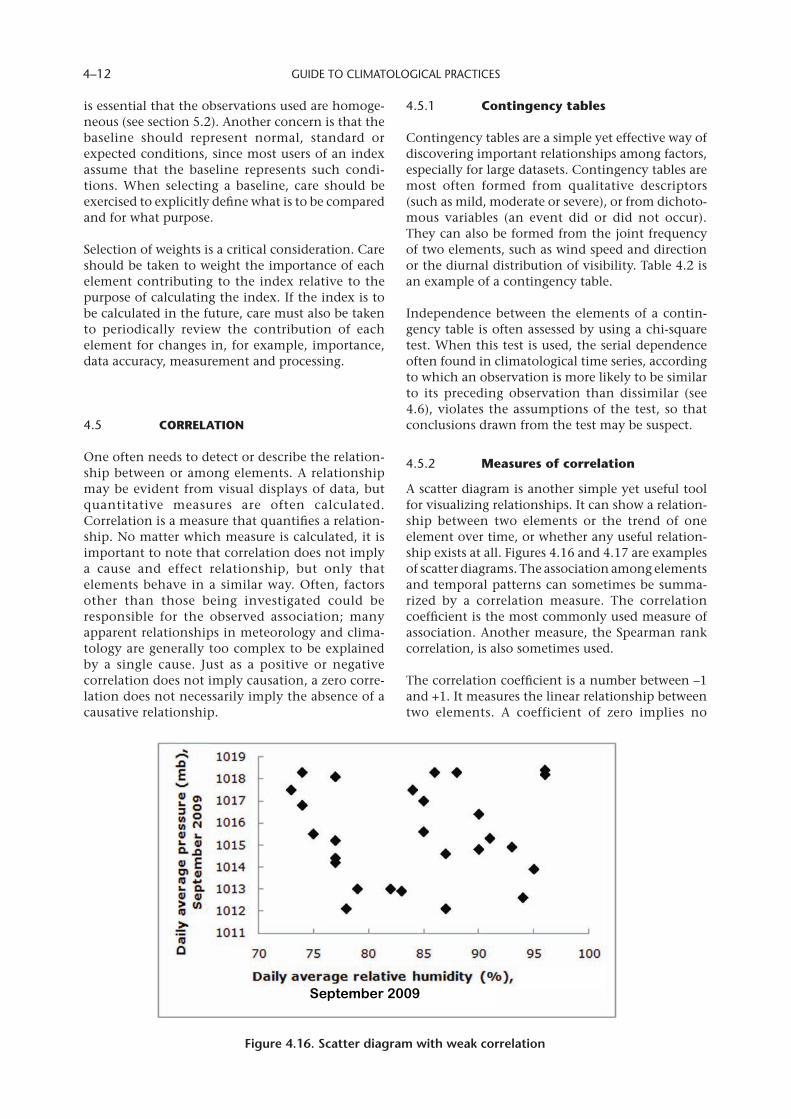
GUIDE TO CLIMATOLOGICAL PRACTICES 4–12
is essential that the observations used are homoge-neous (see section 5.2). Another concern is that the baseline should represent normal, standard or expected conditions, since most users of an index assume that the baseline represents such condi-tions. When selecting a baseline, care should be exercised to explicitly define what is to be compared and for what purpose.
Selection of weights is a critical consideration. Care should be taken to weight the importance of each element contributing to the index relative to the purpose of calculating the index. If the index is to be calculated in the future, care must also be taken to periodically review the contribution of each element for changes in, for example, importance, data accuracy, measurement and processing.
4.5 CORRELATION
One often needs to detect or describe the relation-ship between or among elements. A relationship may be evident from visual displays of data, but quantitative measures are often calculated. Correlation is a measure that quantifies a relation-ship. No matter which measure is calculated, it is important to note that correlation does not imply a cause and effect relationship, but only that elements behave in a similar way. Often, factors other than those being investigated could be responsible for the observed association; many apparent relationships in meteorology and clima-tology are generally too complex to be explained by a single cause. Just as a positive or negative correlation does not imply causation, a zero corre-lation does not necessarily imply the absence of a causative relationship.
4.5.1 Contingencytables
Contingency tables are a simple yet effective way of discovering important relationships among factors, especially for large datasets. Contingency tables are most often formed from qualitative descriptors (such as mild, moderate or severe), or from dichoto-mous variables (an event did or did not occur). They can also be formed from the joint frequency of two elements, such as wind speed and direction or the diurnal distribution of visibility. Table 4.2 is an example of a contingency table.
Independence between the elements of a contin-gency table is often assessed by using a chi-square test. When this test is used, the serial dependence often found in climatological time series, according to which an observation is more likely to be similar to its preceding observation than dissimilar (see 4.6), violates the assumptions of the test, so that conclusions drawn from the test may be suspect.
4.5.2 Measuresofcorrelation
A scatter diagram is another simple yet useful tool for visualizing relationships. It can show a relation-ship between two elements or the trend of one element over time, or whether any useful relation-ship exists at all. Figures 4.16 and 4.17 are examples of scatter diagrams. The association among elements and temporal patterns can sometimes be summa-rized by a correlation measure. The correlation coefficient is the most commonly used measure of association. Another measure, the Spearman rank correlation, is also sometimes used.
The correlation coefficient is a number between –1 and +1. It measures the linear relationship between two elements. A coefficient of zero implies no
September 2009
Figure.4 .16 ..Scatter.diagram.with.weak.correlation
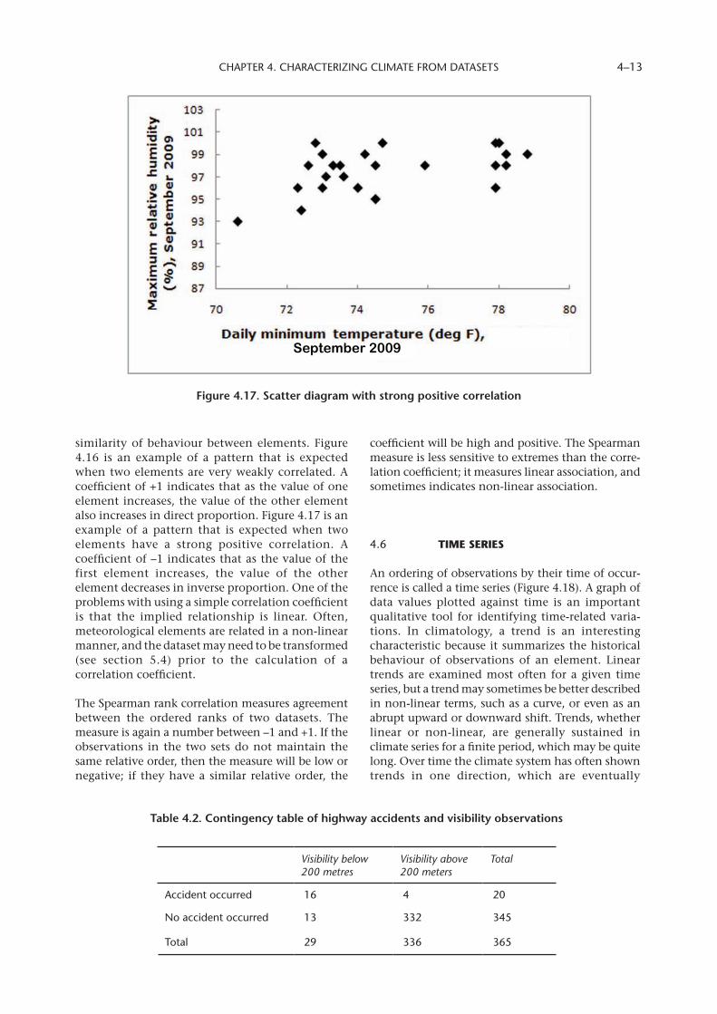
CHAPTER 4. CHARACTERIZING CLIMATE FROM DATASETS 4–13
similarity of behaviour between elements. Figure 4.16 is an example of a pattern that is expected when two elements are very weakly correlated. A coefficient of +1 indicates that as the value of one element increases, the value of the other element also increases in direct proportion. Figure 4.17 is an example of a pattern that is expected when two elements have a strong positive correlation. A coefficient of –1 indicates that as the value of the first element increases, the value of the other element decreases in inverse proportion. One of the problems with using a simple correlation coefficient is that the implied relationship is linear. Often, meteorological elements are related in a non-linear manner, and the dataset may need to be transformed (see section 5.4) prior to the calculation of a correlation coefficient.
The Spearman rank correlation measures agreement between the ordered ranks of two datasets. The measure is again a number between –1 and +1. If the observations in the two sets do not maintain the same relative order, then the measure will be low or negative; if they have a similar relative order, the
coefficient will be high and positive. The Spearman measure is less sensitive to extremes than the corre-lation coefficient; it measures linear association, and sometimes indicates non-linear association.
4.6 TIMESERIES
An ordering of observations by their time of occur-rence is called a time series (Figure 4.18). A graph of data values plotted against time is an important qualitative tool for identifying time-related varia-tions. In climatology, a trend is an interesting characteristic because it summarizes the historical behaviour of observations of an element. Linear trends are examined most often for a given time series, but a trend may sometimes be better described in non-linear terms, such as a curve, or even as an abrupt upward or downward shift. Trends, whether linear or non-linear, are generally sustained in climate series for a finite period, which may be quite long. Over time the climate system has often shown trends in one direction, which are eventually
Figure.4 .17 ..Scatter.diagram.with.strong.positive.correlation
September 2009
Visibility below 200 metres
Visibility above 200 meters
Total
Accident occurred 16 4 20
No accident occurred 13 332 345
Total 29 336 365
Table.4 .2 ..Contingency.table.of.highway.accidents.and.visibility.observations
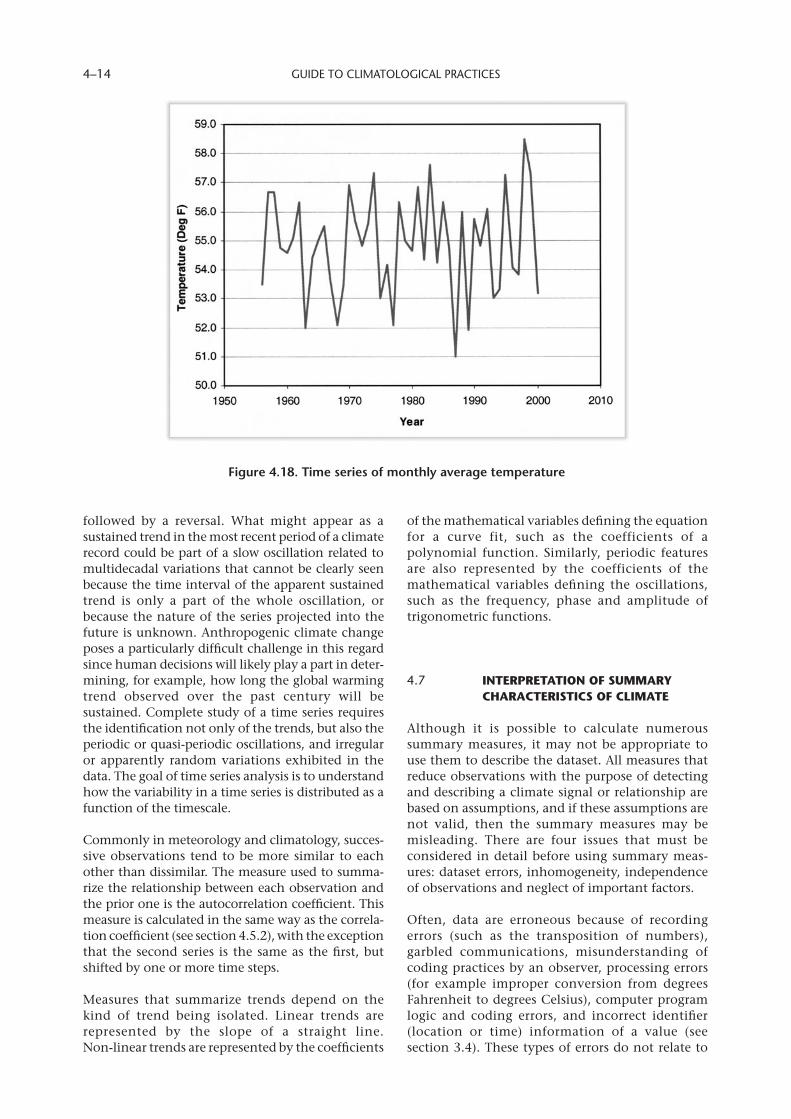
GUIDE TO CLIMATOLOGICAL PRACTICES 4–14
followed by a reversal. What might appear as a sustained trend in the most recent period of a climate record could be part of a slow oscillation related to multidecadal variations that cannot be clearly seen because the time interval of the apparent sustained trend is only a part of the whole oscillation, or because the nature of the series projected into the future is unknown. Anthropogenic climate change poses a particularly difficult challenge in this regard since human decisions will likely play a part in deter-mining, for example, how long the global warming trend observed over the past century will be sustained. Complete study of a time series requires the identification not only of the trends, but also the periodic or quasi-periodic oscillations, and irregular or apparently random variations exhibited in the data. The goal of time series analysis is to understand how the variability in a time series is distributed as a function of the timescale.
Commonly in meteorology and climatology, succes-sive observations tend to be more similar to each other than dissimilar. The measure used to summa-rize the relationship between each observation and the prior one is the autocorrelation coefficient. This measure is calculated in the same way as the correla-tion coefficient (see section 4.5.2), with the exception that the second series is the same as the first, but shifted by one or more time steps.
Measures that summarize trends depend on the kind of trend being isolated. Linear trends are represented by the slope of a straight line. Non-linear trends are represented by the coefficients
of the mathematical variables defining the equation for a curve fit, such as the coefficients of a polynomial function. Similarly, periodic features are also represented by the coefficients of the mathematical variables defining the oscillations, such as the frequency, phase and amplitude of trigonometric functions.
4.7 INTERPRETATIONOFSUMMARYCHARACTERISTICSOFCLIMATE
Although it is possible to calculate numerous summary measures, it may not be appropriate to use them to describe the dataset. All measures that reduce observations with the purpose of detecting and describing a climate signal or relationship are based on assumptions, and if these assumptions are not valid, then the summary measures may be misleading. There are four issues that must be considered in detail before using summary meas-ures: dataset errors, inhomogeneity, independence of observations and neglect of important factors.
Often, data are erroneous because of recording errors (such as the transposition of numbers), garbled communications, misunderstanding of coding practices by an observer, processing errors (for example improper conversion from degrees Fahrenheit to degrees Celsius), computer program logic and coding errors, and incorrect identifier (location or time) information of a value (see section 3.4). These types of errors do not relate to
Figure.4 .18 ..Time.series.of.monthly.average.temperature
CHAPTER 4. CHARACTERIZING CLIMATE FROM DATASETS 4–15
the physical conditions being observed, and they can contaminate data so that improper conclusions are drawn from a data analysis.
Faulty inferences are often made when quantitative measures are used to compare data that are not really comparable, such as when comparing inho-mogeneous observations. If possible, any dataset being analysed should be made homogeneous (see section 5.2).
Many meteorological datasets violate the assump-tion of independence. Prior to summarizing a dataset, care should be taken to remove, if possible, the dependence among observations. For example, the effect of known annual cycles can be largely removed by summarizing departures from the known cycle. For another example, if persistence (autocorrelation) is known to affect a series of obser-vations, as sometimes occurs with daily temperatures observed during a synoptic surface high-pressure event, it should be taken into account by the analyti-cal model. If dependencies are not accounted for by the models, subsampling by selecting only one observation of the several available during the persistent event would remove the persistence affect-ing all the observations taken during the event. Care must also be exercised in this process, however, so as not to introduce aliasing (an effect that causes differ-ent signals to be indistinguishable when sampled), which can lead to an incorrect analysis of any under-lying oscillations.
An incomplete or erroneous explanation can result from presenting quantitative evidence concerning only one factor while ignoring other important factors. An example is comparing temperatures over a cold season at a coastal location and a conti-nental location. The averages may be similar enough to suggest that the climates are the same, but such a conclusion would not be drawn if the greater variability at the continental location were not ignored.
Specific statistical assumptions concerning, for example, the consistency and homogeneity of the data or the nature of the dependence between observations, are implicit in all statistical analysis techniques. These assumptions should be clearly identified and assessed by the analyst, and the interpretation of a summary measure should be tempered by the extent to which the assumptions are satisfied. If any of the assumptions are violated, then the interpretation of a summary measure should be changed to account for the violations. The usual interpretation of the measure may still suffice, but the real or suspected violations should be disclosed with the measure. For example, if annual average temperatures are calculated from a dataset that is known from the metadata to be
inhomogeneous, then the assumption that all data are comparable is violated. This violation, and its effect on the calculation of the mean, should be disclosed.
4.8 NORMALS
Climate normals are used for two principal purposes. They serve as a benchmark against which recent or current observations can be compared, including providing a basis for many anomaly-based climate datasets (for example, global mean temperatures). They are also widely used, implicitly or explicitly, as a prediction of the conditions most likely to be experienced in a given location.
Historical practices regarding climate normals (as described in previous editions of this Guide (WMO-No. 100), the Technical Regulations (WMO-No. 49) and the Handbook on CLIMAT and CLIMAT TEMP Reporting (WMO/TD-No. 1188)) date from the first half of the twentieth century. The general recom-mendation was to use 30-year periods of reference. The 30-year period of reference was set as a stand-ard mainly because only 30 years of data were available for summarization when the recommen-dation was first made. The early intent of normals was to allow comparison among observations from around the world. The use of normals as predictors slowly gained momentum over the course of the twentieth century.
Traditionally, climatological normals have focused on the mean value of a climate element over a period of time. As discussed in section 4.4.2, the mean is an incomplete description of the climate, and many applications require information about other aspects of that element’s frequency distribu-tion and statistical behaviour, such as the frequency of extended periods when a value is above a thresh-old. Extreme values of an element over a specified period, and other statistical descriptors of the frequency distribution of an element (such as the standard deviation of daily or monthly values), are useful descriptors of the climate at a location and should be included with datasets of normals.
Many NMHSs calculate daily normals along with monthly and annual normals. Although not required by WMO, daily normals illustrate the non-random pattern of daily variations of an element that cannot be captured with monthly normals. They are calculated by averaging the values of an element for a specified calendar date over a period of time. The observed values are usually smoothed by 3- to 7-day moving averages or binomial smooth-ing to reduce the effects of random high-frequency temporal variability of weather systems. Another
GUIDE TO CLIMATOLOGICAL PRACTICES 4–16
smoothing approach is to fit the series of daily aver-ages calculated from the observations with spline, trigonometric or polynomial smoothing functions, and these smoothed series become the daily normals (see section 5.8).
4.8.1 Periodofcalculation
Under the WMO Technical Regulations, climatological standard normals are averages of climatological data computed for the following consecutive periods of 30 years: 1 January 1901 to 31 December 1930, 1 January 1931 to 31 December 1960, and so forth. Countries should calculate climatological standard normals as soon as possible after the end of a standard normal period. It is also recommended that, where possible, the calculation of anomalies be based on climatological standard normal periods, in order to allow a uniform basis for comparison. Averages (also known as provisional normals) may be calculated at any time for stations not having 30 years of available data (see 4.8.4). Period averages are aver-ages computed for any period of at least ten years starting on 1 January of a year ending with the digit 1 (for example, 1 January 1991 to 31 December 2004). Although not required by WMO, some countries calculate period averages every decade.
Where climatological standard normals are used as a reference, there are no clear advantages to updat-ing the normals frequently unless an update provides normals for a significantly greater number of stations. Frequent updating carries the disadvan-tage that it requires recalculation not only of the normals themselves, but also numerous datasets that use the normals as a reference. For example, global temperature datasets have been calculated as anomalies from a reference period such as 1961–1990 (Figure 4.19). Using a more recent averaging period, such as 1971–2000, results in a slight improvement in ”predictive accuracy” for elements that show a secular trend (that is, where the time series shows a consistent rise or fall in its values when measured over a long term). Also, 1971–2000 normals would be viewed by many users as more “current” than 1961–1990. The disadvantages of frequent updating, however, could be considered to offset this advantage when the normals are being used for reference purposes.
A number of studies have found that 30 years is not generally the optimal averaging period for normals used for prediction. The optimal period for temperatures is often substantially shorter than 30 years, but the optimal period for precipitation is often substantially greater than 30 years. The Role of Climatological Normals in a Changing Climate (WMO/TD-No. 1377) and other references at the end of this chapter provide much detail on the predictive use of normals of several elements.
Secular trends reduce the representativeness of historical data as a descriptor of the current, or likely future, climate at a given location. Furthermore, the existence of multidecadal varia-bility in the climate system causes differences in climate normals from one reference period to the next such that the representativeness of any given normal for the present climate is reduced. For predictive uses, NMHSs are encouraged to prepare averages and period averages. The optimal length of record for predictive use of normals varies with element, geography and secular trend. In general, the most recent 5- to 10-year period of record has as much predictive value as a 30-year record. Shorter reference periods allow normals to be calculated for a much wider range of stations than is usually possible for a standard normals reference period. For elements that show a substantial underlying trend (such as mean temperature), predictive accu-racy is improved by updating the averages and period averages frequently.
In any publication of normals and averages, and also in any publication that uses them for analysis and display of climate variability, it is important to document the period used for the calculation and the calculation methodologies. The CLIMAT and CLIMAT SHIP codes contain a provision for a start year and an end year to be incorporated in normals distributed through such messages.
4.8.2 Stationsforwhichnormalsandaveragesarecalculated
Climate normals and averages should be calculated for as wide a range of stations as possible, subject to the requirement that a station meet standards for the amount and completeness of available data. As a minimum, they should be calculated, if possible, for all stations whose data are distributed on the Global Telecommunication System (section B.1.3.1.2 of the Technical Regulations).
4.8.3 Homogeneityofdata
As far as possible, the data used in the calculation of climate normals and averages should be homoge-neous. The issue of homogeneity is addressed more fully in section 5.2. In the context of climate normals and averages, homogeneity issues that require particular attention are changes of site loca-tion; changes of observation procedure, including changes of observation time; changes of instrument type; changes of instrument exposure over time; and changes in the processing of data.
In practice, at many locations it will not be possible to construct a suitably homogenous dataset. It may instead be necessary to produce normals from a composite of two or more parts of an inhomogene-
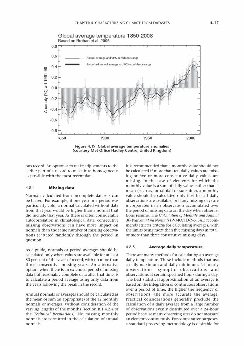
CHAPTER 4. CHARACTERIZING CLIMATE FROM DATASETS 4–17
ous record. An option is to make adjustments to the earlier part of a record to make it as homogeneous as possible with the most recent data.
4.8.4 Missingdata
Normals calculated from incomplete datasets can be biased. For example, if one year in a period was particularly cold, a normal calculated without data from that year would be higher than a normal that did include that year. As there is often considerable autocorrelation in climatological data, consecutive missing observations can have more impact on normals than the same number of missing observa-tions scattered randomly through the period in question.
As a guide, normals or period averages should be calculated only when values are available for at least 80 per cent of the years of record, with no more than three consecutive missing years. An alternative option, when there is an extended period of missing data but reasonably complete data after that time, is to calculate a period average using only data from the years following the break in the record.
Annual normals or averages should be calculated as the mean or sum (as appropriate) of the 12 monthly normals or averages, without consideration of the varying lengths of the months (section B.1.4.2.4 of the Technical Regulations). No missing monthly normals are permitted in the calculation of annual normals.
It is recommended that a monthly value should not be calculated if more than ten daily values are miss-ing or five or more consecutive daily values are missing. In the case of elements for which the monthly value is a sum of daily values rather than a mean (such as for rainfall or sunshine), a monthly value should be calculated only if either all daily observations are available, or if any missing days are incorporated in an observation accumulated over the period of missing data on the day when observa-tions resume. The Calculation of Monthly and Annual 30-Year Standard Normals (WMO/TD-No. 341) recom-mends stricter criteria for calculating averages, with the limits being more than five missing days in total, or more than three consecutive missing days.
4.8.5 Averagedailytemperature
There are many methods for calculating an average daily temperature. These include methods that use a daily maximum and daily minimum, 24 hourly observations, synoptic observations and observations at certain specified hours during a day. The best statistical approximation of an average is based on the integration of continuous observations over a period of time; the higher the frequency of observations, the more accurate the average. Practical considerations generally preclude the calculation of a daily average from a large number of observations evenly distributed over a 24-hour period because many observing sites do not measure an element continuously. For comparative purposes, a standard processing methodology is desirable for
Figure.4 .19 ..Global.average.temperature.anomalies..(courtesy.Met.Office.Hadley.Centre,.United.Kingdom)
GUIDE TO CLIMATOLOGICAL PRACTICES 4–18
all stations worldwide, with the number of stations maximized.
All ordinary climatological stations observe a daily maximum and minimum temperature (see section 2.2.1). Hence, the recommended method-ology for calculating average daily temperature is to take the mean of the daily maximum and minimum temperatures. Even though this method is not the best statistical approximation, its consistent use satisfies the comparative purpose of normals. An NMHS should also calcu-late daily averages using other methods if these calculations improve the understanding of the climate of the country.
4.8.6 Precipitationquintiles
Quintiles of precipitation are used to relate an observed monthly precipitation total to the frequency distribution of values observed over the period for which normals have been calculated. No universally accepted method exists for the calcula-tion of quintile boundaries, and the choice of method can make a substantial difference to the calculated values. The recommended procedure for calculating the boundaries, however, is as follows:
For any month the 30 monthly values of precipita-tion recorded during the 30-year normal period are listed in ascending order. The list is then divided into five groups of quintiles of six values each. The first quintile contains the six lowest values for the month in question that have been observed during the 30-year period, the second quintile the next six lowest values, and so on to the fifth quintile, which contains the six highest values.
The boundary between two adjacent quintiles is set halfway between the top value of the one quintile and the first value of the next. The quintile index is the number of the lowest quintile containing the monthly precipitation in the month for which the report is being prepared, with the following special rules:(a) If the precipitation is 0: use index 0 if this has
not occurred during the reference period; use 1 if it has occurred but fewer than 6 times; use 2 if it has occurred between 7 and 12 times; use 3 if it has occurred 13 to 18 times, and so on;
(b) If the precipitation is less than any value in the reference period: use index 0 (regardless of whether the precipitation is 0);
(c) If the precipitation is greater than any value in the reference period: use index 6.
4.8.7 Disseminationofnormals
A main avenue for international dissemination of climate normals is through CLIMAT (for land-based
surface stations) and CLIMAT SHIP (for ship-based surface observations) coded messages sent on the Global Telecommunication System. Coding and reporting procedures are described in the Handbook on CLIMAT and CLIMAT TEMP Reporting (WMO/TD-No. 1188).
4.9 REFERENCESANDADDITIONALREADING
4.9.1 WMOpublications
World Meteorological Organization, 1983: Guide to Climatological Practices. Second edition (WMO-No. 100), Geneva.
———, 1988: Technical Regulations, Vol. I – General Meteorological Standards and Recommended Practices; Vol. II – Meteorological Service for International Air Navigation; Vol. III – Hydrology (WMO-No. 49), Geneva.
———, 1989: Calculation of Monthly and Annual 30-Year Standard Normals (WMO/TD-No. 341, WCDP-No. 10), Geneva.
———, 1990: On the Statistical Analysis of Series of Observations (WMO/TN-No. 143, WMO-No. 415), Geneva.
———, 1995: Manual on Codes (WMO-No. 306), Geneva.
———, 1996: Climatological Normals (CLINO) for the Period 1961–90 (WMO-No. 847), Geneva.
———, 2004: Handbook on CLIMAT and CLIMAT TEMP Reporting (WMO/TD-No. 1188), Geneva.
———, 2007: The Role of Climatological Normals in a Changing Climate (WMO/TD-No. 1377, WCDMP-No. 61), Geneva.
4.9.2 Additionalreading
Angel, J.R., W.R. Easterling and S.W. Kirtsch, 1993: Towards defining appropriate averaging periods for climate normals. Clim. Bull., 27:29–44.
Asnani, G.C., 1993: Tropical Meteorology (2 vols.), Pune, Sind Society.
Barnston, A.G. and R.E. Livezey, 1987: Classification, seasonality and persistence of low-frequency atmospheric circulation patterns. Monthly Weather Rev., 115:1083–1126.
Bhalme, H.N. and D.A. Mooley, 1980: Large-scale droughts/floods and monsoon circulation. Monthly Weather Rev., 108:1197–1211.
Bhalme, H.N., D.A. Mooley and S.K. Jadhav, 1984: Large-scale April pressure index connected with the southern oscillation and its potential for prediction of large-scale droughts over India. Mausam, 35(3):355–360.
Brohan, P., J.J. Kennedy, I. Harris, S.F.B. Tett and P.D. Jones, 2006: Uncertainty estimates in regional and global observed temperature
CHAPTER 4. CHARACTERIZING CLIMATE FROM DATASETS 4–19
Rao, G.A., S.V. Datar and H.N. Srivastava, 1992: Study of drought indices in relation to rice crop production over some States of India. Mausam, 43(2):169–174.
Srivastava, A.K., P. Guhathakurta and S.R. Kshirsagar, 2003: Estimation of annual and seasonal temperatures over Indian stations using opti-mal normals. Mausam, 54:615–622.
Tukey, J.W., 1977: Exploratory Data Analysis. Reading, Massachusetts, Addison Wesley.
Von Storch, H. and F.W. Zwiers, 1999: Statistical Analysis in Climate Research. Cambridge, Cambridge University Press.
Wilks, D.S., 1995: Statistical Methods in the Atmospheric Sciences. San Diego, Academic Press.
changes: a new dataset from 1850. J. Geophysical Research 111, D12106.
Dixon, K.W. and M.D. Shulman, 1984: A statistical evaluation of the predictive abilities of climatic averages. J. Clim. Appl. Meteorol., 23:1542–1552.
Guttman, N.B., 1989: Statistical descriptors of climate. Bull. Amer. Meteor. Soc., 70:602–607.
Huang, J., H.M. van den Dool and A.G. Barnston, 1996: Long-lead seasonal temperature prediction using optimal climate normals. J. Climate, 9:809–817.
Lamb, P.J. and S.A. Changnon, 1981: On the “best” temperature and precipitation normals: the Illinois situation. J. Appl. Meteorol., 20:1383–1390.
Matheron, G., 1973: The intrinsic random functions and their applications. Adv. Appl. Prob., 5:207–221.
.
����STATISTICAL.METHODS.FOR.ANALYSING.DATASETS
CHAPTER 5
5.1 INTRODUCTION
This chapter introduces some of the statistical concepts and methods available to climatologists, but does not provide detailed specifics of complex subjects. Some statistical methods are given only cursory treatment, while others are ignored. The references at the end of the chapter and textbooks on statistical theory and methods provide more detailed information. Two references that should be on every climatologist’s bookshelf are Some Methods in Climatological Analysis (WMO-No. 199) and On the Statistical Analysis of Series of Observations (WMO-No. 415). Since new and improved statisti-cal and analytical methodologies are rapidly emerging, climatologists should maintain aware-ness of current techniques that have practical applications in climatology.
The main interest in the use of observed meteoro-logical or climatological data is not to describe the data (see Chapter 4), but to make inferences from a limited representation (the observed sample of data) of complex physical events that are helpful to users of climatological information. The interpreta-tion of climatological data usually involves both spatial and temporal comparisons among charac-teristics of frequency distributions both. These comparisons answer common questions such as:Are average temperatures taken over a specific time interval at different locations the same?(a) Is the variability of precipitation the same at
different locations?(b) Is the diurnal temperature range at a location
changing over time, and if so, how?(c) What is the likelihood of occurrence of tropi-
cal storms in an area?
Inferences are based directly on probability theory, and the use of statistical methods to make infer-ences is therefore based on formal mathematical reasoning. Statistics can be defined as the pure and applied science of creating, developing and applying techniques such that the uncertainty of inductive inferences may be evaluated. Statistics is the tool used to bridge the gap between the raw data and useful information, and it is used for analysing data and climate models and for climate prediction. Statistical methods allow a statement of the confidence of any decision based on applica-tion of the procedures.
The confidence that can be placed in a decision is important because of the risks that might be
associated with making a wrong decision. Observed data represent only a single realization of the physical system of climate and weather, and, further, are generally observed with some level of error. Conclusions can be correct or incorrect. Quantitative factors that describe the confidence of the decisions are therefore necessary to properly use the information contained in a dataset.
5.2 HOMOGENIZATION
Analysis of climate data to detect changes and trends is more reliable when homogenized datasets are used. A homogeneous climate dataset is one in which all the fluctuations contained in its time series reflect the actual variability and change of the represented climate element. Most statistical meth-ods assume the data under examination are as free from instrumentation, coding, processing and other non-meteorological or non-climatological errors as possible. Meteorological or climatological data, however, are generally not homogeneous nor are they free from error. Errors range from system-atic (they affect a whole set of observations the same way, such as constant instrument calibration errors or improper conversion of units), to random (any one observation is subject to an error that is as likely to be positive as negative, such as parallax differences among observers reading a mercury barometer).
The best way to keep the record homogeneous is to avoid changes in the collection, handling, trans-mission and processing of the data. It is highly advisable to maintain observing practices and instruments as unchanged as possible (Guide to the GCOS Surface and Upper-Air Networks: GSN AND GUAN, WMO/TD-No. 1106). Unfortunately, most long-term climatological datasets have been affected by a number of factors not related to the broader-scale climate. These include, among other things, changes in geographical location; local land use and land cover; instrument types, exposure, mounting and sheltering; observing practices; calculations, codes and units; and historical and political events. Some changes may cause sharp discontinuities such as steps (for example, a change in instrument or site), while others may cause grad-ual biases (for example, increasing urbanization in the vicinity of a site). In both cases, the related time series become inhomogeneous, and these inhomo-geneities may affect the proper assessment of
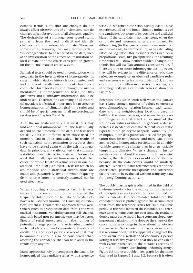
GUIDE TO CLIMATOLOGICAL PRACTICES 5–2
climatic trends. Note that site changes do not always affect observations of all elements, nor do changes affect observations of all elements equally. The desirability of a homogeneous record stems primarily from the need to distil and identify changes in the broader-scale climate. There are some studies, however, that may require certain “inhomogeneities” to be reflected in the data, such as an investigation of the effects of urbanization on local climate or of the effects of vegetation growth on the microclimate of an ecosystem.
Statistical tests should be used in conjunction with metadata in the investigation of homogeneity. In cases in which station history is documented well and sufficient parallel measurements have been conducted for relocations and changes of instru-mentation, a homogenization based on this qualitative and quantitative information should be undertaken. Therefore, the archiving of all histori-cal metadata is of critical importance for an effective homogenization of climatological time series and should be of special concern to all meteorological services (see Chapters 2 and 3).
After the metadata analysis, statistical tests may find additional inhomogeneities. The tests usually depend on the timescale of the data; the tests used for daily data are different from those used for monthly data or other timescales. The results of such statistical homogenization procedures then have to be checked again with the existing meta-data. In principle, any statistical test that compares a statistical parameter of two data samples may be used. But usually, special homogeneity tests that check the whole length of a time series in one run are used. Both non-parametric tests (in which no assumptions about statistical distributions are made) and parametric tests (in which frequency distribution is known or correctly assumed) can be used effectively.
When choosing a homogeneity test, it is very important to keep in mind the shape of the frequency distribution of the data. Some datasets have a bell-shaped (normal or Gaussian) distribu-tion; for these a parametric approach works well. Others (such as precipitation data from a site with marked interannual variability) are not bell- shaped, and rank-based non-parametric tests may be better. Effects of serial autocorrelation, the number of potential change points in a series (documented with metadata and undocumented), trends and oscillations, and short periods of record that may be anomalous should also be considered when assessing the confidence that can be placed in the results from any test.
Many approaches rely on comparing the data to be homogenized (the candidate series) with a reference
series. A reference time series ideally has to have experienced all of the broad climatic influences of the candidate, but none of its possible and artificial biases. If the candidate is homogeneous, when the candidate and reference series are compared by differencing (in the case of elements measured on an interval scale, like temperature) or by calculating ratios or log ratios (for elements measured on a proportional scale, like precipitation), the resulting time series will show neither sudden changes nor trends, but will oscillate around a constant value. If there are one or more inhomogeneities, however, they will be evident in the difference or ratio time series. An example of an observed candidate series and a reference series is shown in Figure 5.1, and an example of a difference series revealing an inhomogeneity in a candidate series is shown in Figure 5.2.
Reference time series work well when the dataset has a large enough number of values to ensure a good climatological relation between each candi-date and the neighbouring locations used in building the reference series, and when there are no inhomogeneities that affect all or most of the stations or values available. In general, a denser network is needed for climatic elements or climatic types with a high degree of spatial variability (for examples, more data points are needed for precipi-tation than for temperature, and more data points are needed to homogenize precipitation in a highly variable temperature climate than in a less variable temperature climate). When a change in instru-ments occurs at about the same time in an entire network, the reference series would not be effective because all the data points would be similarly affected. When a suitable reference series cannot be constructed, possible breakpoints and correction factors need to be evaluated without using any data from neighbouring stations.
The double-mass graph is often used in the field of hydrometeorology for the verification of measures of precipitation and runoff, but can be used for most elements. The accumulated total from the candidate series is plotted against the accumulated total from the reference series for each available period. If the ratio between the candidate and refer-ence series remains constant over time, the resultant double-mass curve should have constant slope. Any important variation in the slope or the shape of the curve indicates a change in the relationship between the two series. Since variations may occur naturally, it is recommended that the apparent changes of the slope occur for a well-defined continuous period lasting at least five years and that they be consistent with events referenced in the metadata records of the station before concluding inhomogeneity. Figure 5.3 shows a double-mass graph for the same data used in Figures 5.1 and 5.2. Because it is often
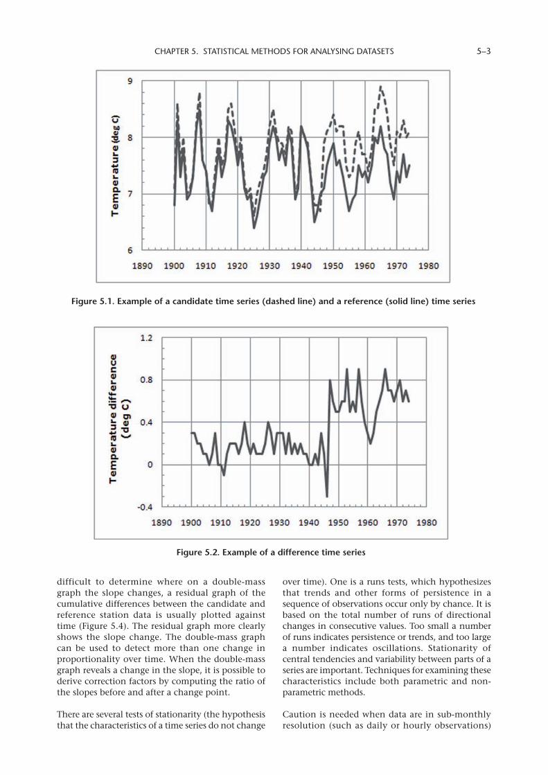
CHAPTER 5. STATISTICAL METHODS FOR ANALYSING DATASETS 5–3
over time). One is a runs tests, which hypothesizes that trends and other forms of persistence in a sequence of observations occur only by chance. It is based on the total number of runs of directional changes in consecutive values. Too small a number of runs indicates persistence or trends, and too large a number indicates oscillations. Stationarity of central tendencies and variability between parts of a series are important. Techniques for examining these characteristics include both parametric and non-parametric methods.
Caution is needed when data are in sub-monthly resolution (such as daily or hourly observations)
difficult to determine where on a double-mass graph the slope changes, a residual graph of the cumulative differences between the candidate and reference station data is usually plotted against time (Figure 5.4). The residual graph more clearly shows the slope change. The double-mass graph can be used to detect more than one change in proportionality over time. When the double-mass graph reveals a change in the slope, it is possible to derive correction factors by computing the ratio of the slopes before and after a change point.
There are several tests of stationarity (the hypothesis that the characteristics of a time series do not change
Figure.5 .1 ..Example.of.a.candidate.time.series.(dashed.line).and.a.reference.(solid.line).time.series
Figure.5 .2 ..Example.of.a.difference.time.series
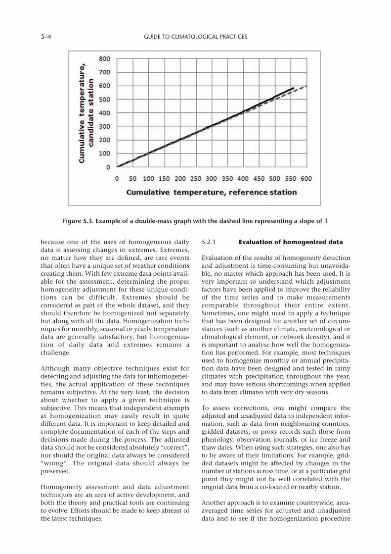
GUIDE TO CLIMATOLOGICAL PRACTICES 5–4
because one of the uses of homogeneous daily data is assessing changes in extremes. Extremes, no matter how they are defined, are rare events that often have a unique set of weather conditions creating them. With few extreme data points avail-able for the assessment, determining the proper homogeneity adjustment for these unique condi-tions can be difficult. Extremes should be considered as part of the whole dataset, and they should therefore be homogenized not separately but along with all the data. Homogenization tech-niques for monthly, seasonal or yearly temperature data are generally satisfactory, but homogeniza-tion of daily data and extremes remains a challenge.
Although many objective techniques exist for detecting and adjusting the data for inhomogenei-ties, the actual application of these techniques remains subjective. At the very least, the decision about whether to apply a given technique is subjective. This means that independent attempts at homogenization may easily result in quite different data. It is important to keep detailed and complete documentation of each of the steps and decisions made during the process. The adjusted data should not be considered absolutely “correct”, nor should the original data always be considered “wrong”. The original data should always be preserved.
Homogeneity assessment and data adjustment techniques are an area of active development, and both the theory and practical tools are continuing to evolve. Efforts should be made to keep abreast of the latest techniques.
5.2.1 Evaluationofhomogenizeddata
Evaluation of the results of homogeneity detection and adjustment is time-consuming but unavoida-ble, no matter which approach has been used. It is very important to understand which adjustment factors have been applied to improve the reliability of the time series and to make measurements comparable throughout their entire extent. Sometimes, one might need to apply a technique that has been designed for another set of circum-stances (such as another climate, meteorological or climatological element, or network density), and it is important to analyse how well the homogeniza-tion has performed. For example, most techniques used to homogenize monthly or annual precipita-tion data have been designed and tested in rainy climates with precipitation throughout the year, and may have serious shortcomings when applied to data from climates with very dry seasons.
To assess corrections, one might compare the adjusted and unadjusted data to independent infor-mation, such as data from neighbouring countries, gridded datasets, or proxy records such those from phenology, observation journals, or ice freeze and thaw dates. When using such strategies, one also has to be aware of their limitations. For example, grid-ded datasets might be affected by changes in the number of stations across time, or at a particular grid point they might not be well correlated with the original data from a co-located or nearby station.
Another approach is to examine countrywide, area-averaged time series for adjusted and unadjusted data and to see if the homogenization procedure
Figure.5 .3 ..Example.of.a.double-mass.graph.with.the.dashed.line.representing.a.slope.of.1
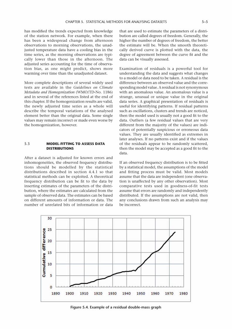
CHAPTER 5. STATISTICAL METHODS FOR ANALYSING DATASETS 5–5
has modified the trends expected from knowledge of the station network. For example, when there has been a widespread change from afternoon observations to morning observations, the unad-justed temperature data have a cooling bias in the time series, as the morning observations are typi-cally lower than those in the afternoon. The adjusted series accounting for the time of observa-tion bias, as one might predict, shows more warming over time than the unadjusted dataset.
More complete descriptions of several widely used tests are available in the Guidelines on Climate Metadata and Homogenization (WMO/TD-No. 1186) and in several of the references listed at the end of this chapter. If the homogenization results are valid, the newly adjusted time series as a whole will describe the temporal variations of the analysed element better than the original data. Some single values may remain incorrect or made even worse by the homogenization, however.
5.3 MODEL-FITTINGTOASSESSDATADISTRIBUTIONS
After a dataset is adjusted for known errors and inhomogeneities, the observed frequency distribu-tions should be modelled by the statistical distributions described in section 4.4.1 so that statistical methods can be exploited. A theoretical frequency distribution can be fit to the data by inserting estimates of the parameters of the distri-bution, where the estimates are calculated from the sample of observed data. The estimates can be based on different amounts of information or data. The number of unrelated bits of information or data
that are used to estimate the parameters of a distri-bution are called degrees of freedom. Generally, the higher the number of degrees of freedom, the better the estimate will be. When the smooth theoreti-cally derived curve is plotted with the data, the degree of agreement between the curve fit and the data can be visually assessed.
Examination of residuals is a powerful tool for understanding the data and suggests what changes to a model or data need to be taken. A residual is the difference between an observed value and the corre-sponding model value. A residual is not synonymous with an anomalous value. An anomalous value is a strange, unusual or unique value in the original data series. A graphical presentation of residuals is useful for identifying patterns. If residual patterns such as oscillations, clusters and trends are noticed, then the model used is usually not a good fit to the data. Outliers (a few residual values that are very different from the majority of the values) are indi-cators of potentially suspicious or erroneous data values. They are usually identified as extremes in later analyses. If no patterns exist and if the values of the residuals appear to be randomly scattered, then the model may be accepted as a good fit to the data.
If an observed frequency distribution is to be fitted by a statistical model, the assumptions of the model and fitting process must be valid. Most models assume that the data are independent (one observa-tion is unaffected by any other observation). Most comparative tests used in goodness-of-fit tests assume that errors are randomly and independently distributed. If the assumptions are not valid, then any conclusions drawn from such an analysis may be incorrect.
Figure.5 .4 ..Example.of.a.residual.double-mass.graph
GUIDE TO CLIMATOLOGICAL PRACTICES 5–6
Once the data have been fitted by an acceptable statistical frequency distribution, meeting any necessary independence, randomness or other sampling criteria, and the fit has been validated (see section 4.4), the model can be used as a representa-tion of the data. Inferences can be made that are supported by mathematical theory. The model provides estimates of central tendency, variability and higher-order properties of the distribution (such as skewness or kurtosis). The confidence that these sample estimates represent real physical conditions can also be determined. Other charac-teristics, such as the probability of an observation’s exceeding a given value, can also be estimated by applying both probability and statistical theory to the modelled frequency distribution. All of these tasks are much harder, if not impossible, when using the original data rather than the fitted frequency distribution.
5.4 DATATRANSFORMATION
The normal or Gaussian frequency distribution is widely used, as it has been studied extensively in statistics. If the data do not fit the normal distribu-tion well, applying a transform to the data may result in a frequency distribution that is nearly normal, allowing the theory underlying the normal distribution to form the basis for many inferential uses. Transforming data must be done with care so that the transformed data still represent the same physical processes as the original data and that sound conclusions can be made.
There are several ways to tell whether a distribution of an element is substantially non-normal. A visual inspection of histograms, scatter plots, or probability–probability (P–P) or quantile–quantile (Q–Q) plots is relatively easy to perform. A more objective assess-ment can range from simple examination of skewness and kurtosis (see section 4.4) to inferential tests of normality.
Prior to applying any transformation, an analyst must make certain that the non-normality is caused by a valid reason. Invalid reasons for non-normal-ity include mistakes in data entry and missing data values not declared missing. Another invalid reason for non-normality may be the presence of outliers, as they may well be a realistic part of a normal distribution.
The most common data transformations utilized for improving normality are the square root, cube root, logarithmic and inverse transformations. The square root makes values less than 1 relatively greater, and values greater than 1 relatively smaller. If the values can be positive or negative, a constant
offset must be added before taking the square root so that all values are greater than or equal to 0. The cube root has a similar effect to the square root, but does not require the use of an offset to handle nega-tive values. Logarithmic transformations compresses the range of values, by making small values rela-tively larger and large values relatively smaller. A constant offset must first be added if values equal to 0 or lower are present. An inverse makes very small numbers very large and very large numbers very small; values of 0 must be avoided.
These transformations have been described in the relative order of power, from weakest to strongest. A good guideline is to use the minimum amount of transformation necessary to improve normality. If a meteorological or climatological element has an inherent highly non-normal frequency distribu-tion, such as the U-shape distribution of cloudiness and sunshine, there are no simple transformations allowing the normalization of the data.
The transformations all compress the right side of a distribution more than the left side; they reduce higher values more than lower values. Thus, they are effective on positively skewed distributions such as precipitation and wind speed. If a distribu-tion is negatively skewed, it must be reflected (values are multiplied by –1, and then a constant is added to make all values greater than 0) to reverse the distribution prior to applying a transformation, and then reflected again to restore the original order of the element.
Data transformations offer many benefits, but they should be used appropriately in an informed manner. All of the transformations described above attempt to improve normality by reducing the rela-tive spacing of data on the right side of the distribution more than the spacing on the left side. The very act of altering the relative distances between data points, which is how these transfor-mations aim to improve normality, raises issues in the interpretation of the data, however. All data points remain in the same relative order as they were prior to transformation, which allows inter-pretation of results in terms of the increasing value of the element. The transformed distributions will likely become more complex to interpret physi-cally, however, due to the curvilinear nature of the transformations. The analyst must therefore be careful when interpreting results based on trans-formed data.
5.5 TIMESERIESANALYSIS
The principles guiding model-fitting (see section 5.3) also guide time series analysis. A model is fitted
CHAPTER 5. STATISTICAL METHODS FOR ANALYSING DATASETS 5–7
to the data series; the model might be linear, curvi-linear, exponential, periodic or some other mathematical formulation. The best fit (the fit that minimizes the differences between the data series and the model) is generally accomplished by using least-squares techniques (minimizing the sum of squared departures of the data from the curve fit). Residuals from the best fit are examined for patterns, and if patterns are found, then the model is adjusted to incorporate the patterns.
Time series in climatology have been analysed mainly with harmonic and spectral analysis tech-niques that decompose a series into time domain or frequency domain components. A critical assump-tion of these models is that of stationarity (characteristics of the series such as mean and vari-ance do not change over the length of the series). This condition is generally not met by climatologi-cal data even if the data are homogeneous (see section 5.2).
Gabor and wavelet analysis are extensions of the classical techniques of spectral analysis. By allow-ing subintervals of a time series to be modelled with different scales or resolutions, the condition of stationarity is relaxed. These analyses are particu-larly good at representing time series with subintervals that have differing characteristics. Wavelet analysis gives good results when the time series has spikes or sharp discontinuities. Compared to the classical techniques, they are particularly efficient for signals in which both the amplitude and frequency vary with time. One of the main advantages of these “local” analyses is the ability to present time series of climate processes in the coor-dinates of frequency and time, studying and visualizing the evolution of various modes of vari-ability over a long period. They are used not only as a tool for identifying non-stationary scales of varia-tions, but also as a data analysis tool to gain an initial understanding of a dataset. There have been many applications of these methods in climatol-ogy, such as in studies of the El Nino–Southern Oscillation (ENSO) phenomenon, the North Atlantic Oscillation, atmospheric turbulence, space–time precipitation relationships and ocean wave characteristics.
These methods do have some limitations. The most important limitation for wavelet analysis is that an infinite number of wavelet functions are available as a basis for an analysis, and results often differ depending on which wavelet is used. This makes interpretation of results somewhat difficult because different conclusions can be drawn from the same dataset if different mathematical functions are used. It is therefore important to relate the wavelet function to the physical world prior to selecting a specific wavelet. Gabor and wavelet analysis
techniques are emerging fields, and although the mathematics has been defined, future refinements in techniques and application methodology may mitigate the limitations.
Other common techniques for analysing time series are autoregression and moving average analyses. Autoregression is a linear regression of a value in a time series against one or more prior values in the series (autocorrelation). A moving average process expresses an observed series as a function of a random series. A combination of these two meth-ods is called a mixed autoregressive and moving average (ARMA) model. An ARMA model that allows for non-stationarity is called a mixed autore-gressive integrated moving average (ARIMA) model. These regression-based models can be made more complex than necessary, resulting in overfitting. Overfitting can lead to the modelling of a series of values with minimal differences between the model and the data values, but since the data values are only a sample representation of a physical process, a slight lack of fit may be desirable in order to repre-sent the true process. Other problems include non-stationarity of the parameters used to define a model, non-random residuals (indicating an improper model), and periodicity inherent in the data but not modelled. Split validation is effective in detecting model overfitting. Split validation refers to developing a model based on a portion of the available data and then validating the model on the remaining data that were not used in the model development.
Once the time series data have been modelled by an acceptable curve, and the fit validated, the mathe-matical properties of the model curve can be used to make assessments that would not be possible using the original data. These include measuring trends, cyclical behaviour, or autocorrelation and persistence, together with estimates of the confi-dence of these measures.
5.6 MULTIVARIATEANALYSIS
Multivariate datasets are a compilation of observations of more than one element or a compilation of observations of one element at different points in space. These datasets are often studied for many different purposes. The most important purposes are to see if there are simpler ways of representing a complex dataset, if observations fall into groups and can be classified, if the elements fall into groups, and if interdependence exists among elements. Such datasets are also used to test hypotheses about the data. The time order of the observations is generally not a consideration; time series of more than one
GUIDE TO CLIMATOLOGICAL PRACTICES 5–8
element are usually considered as a separate analysis topic with techniques such as cross-spectral analysis.
Principal components analysis, sometimes referred to as empirical orthogonal functions analysis, is a technique for reducing the dimensions of multi-variate data. The process simplifies a complex dataset and has been used extensively in the analy-sis of climatological data. Principal components analysis methods decompose a number of corre-lated observations into a new set of uncorrelated (orthogonal) functions that contain the original variance of the data. These empirical orthogonal functions, also called principal components, are ordered so that the first component is the one explaining most of the variance, the second compo-nent explains the second-largest share of the variance, and so on. Since most of the variance is usually explained by just a few components, the methods are effective in reducing “noise” from an observed field. Individual components can often be related to a single meteorological or climatological element. The method has been used to analyse a diversity of fields that include sea surface tempera-tures, regional land temperature and precipitation patterns, tree-ring chronologies, sea level pressure, air pollutants, radiative properties of the atmos-phere, and climate scenarios. Principal components have also been used as a climate reconstruction tool, such as in estimating a spatial grid of a climatic element from proxy data when actual observations of the element are not available.
Factor analysis reduces a dataset from a larger set of observations to a smaller set of factors. In the mete-orological and climatological literature, factor analysis is often called rotated principal compo-nents analysis. It is similar to principal components analysis except that the factors are not uncorre-lated. Since a factor may represent observations from more than one element, meteorological or climatological interpretation of a factor is often difficult. The method has been used mainly in synoptic climatology studies.
Cluster analysis attempts to separate observations into groups with similar characteristics. There are many methods for clustering, and different meth-ods are used to detect different patterns of points. Most of the methods, however, rely on the extent to which the distance between means of two groups is greater than the mean distance within a group. The measure of distance does not need to be the usual Euclidean distance, but it should obey certain criteria. One such criterion should be that the meas-ure of distance from point A to point B is equal to the distance from point B to point A (symmetry). A second criterion is that the distance should be a positive value (non-negativity). A third criterion is
that for three points forming a triangle, the length of one side should be less than or equal to the sum of the lengths of the other two sides (triangle inequality). A fourth criterion should be that if the distance from A to B is zero, then A and B are the same (definiteness). Most techniques iteratively separate the data into more and more clusters, thereby presenting the problem for the analyst of determining when the number of clusters is suffi-cient. Unfortunately, there are no objective rules for making this decision. The analyst should there-fore use prior knowledge and experience in deciding when a meteorologically or climatologically appro-priate number of clusters has been obtained. Cluster analysis has been used for diverse purposes, such as constructing homogeneous regions of precipita-tion, analysing synoptic climatologies, and predicting air quality in an urban environment.
Canonical correlation analysis seeks to determine the interdependence between two groups of elements. The method finds the linear combination of the distribution of the first element that produces the correlation with the second distribution. This linear combination is extracted from the dataset and the process is repeated with the residual data, with the constraint that the second linear combina-tion is not correlated with the first combination. The process is again repeated until a linear combi-nation is no longer significant. This analysis is used, for example, in making predictions from telecon-nections, in statistical downscaling (see section 6.7.3), in determining homogeneous regions for flood forecasting in an ungauged basin, and in reconstructing spatial wind patterns from pressure fields.
These methods all have assumptions and limita-tions. The interpretation of the results is very much dependent on the assumptions being met and on the experience of the analyst. Other methods, such as multiple regression and covariance analysis, are even more restrictive for most meteorological or climatological data. Multivariate analysis is complex, with numerous possible outcomes, and requires care in its application.
5.7 COMPARATIVEANALYSIS
By fitting a model function to the data, be it a frequency distribution or a time series, it is possible to use the characteristics of that model for further analysis. The properties of the model characteristics are generally well studied, allowing a range of conclusions to be drawn. If the characteristics are not well studied, bootstrapping may be useful. Bootstrapping is the estimation of model character-istics from multiple random samples drawn from
CHAPTER 5. STATISTICAL METHODS FOR ANALYSING DATASETS 5–9
the original observational series. It is an alternative to making inferences from parameter-based assumptions when the assumptions are in doubt, when parametric inference is impossible, or when parametric inference requires very complicated formulas. Bootstrapping is simple to apply, but it may conceal its own set of assumptions that would be more formally stated in other approaches.
In particular, there are many tests available for comparing the characteristics of two models to determine how much confidence can be placed in claims that the two sets of modelled data share underlying characteristics. When comparing two models, the first step is to decide which characteris-tics are to be compared. These could include the mean, median, variance or probability of an event from a distribution, or the phase or frequency from a time series. In principle, any computable charac-teristic of the fitted models can be compared, although there should be some meaningful reason (based on physical arguments) to do so.
The next step is to formulate the null hypothesis. This is the hypothesis considered to be true before any testing is done, and in this case it is usually that the modelled characteristics are the same. The alter-native hypothesis is the obverse, that the modelled characteristics are not the same.
A suitable test to compare the characteristics from the two models is then selected. Some of these tests are parametric, depending on assumptions about the distribution, such as normality. Parametric tests include the Student’s t-test (for comparing means) and the Fisher’s F-test (for comparing variability). Other tests are non-parametric, so they do not make assumptions about the distribution. They include sign tests (for comparing medians) and the Kolmogorov-Smirnov test for comparing distribu-tions. Parametric tests are generally better (in terms of confidence in the conclusions), but only if the required assumptions about the distribution are valid.
The seriousness of rejecting a true hypothesis (or accepting a false one) is expressed as a level of confi-dence or probability. The selected test will show whether the null hypothesis can be accepted at the level of confidence required. Some of the tests will reveal at what level of confidence the null hypoth-esis can be accepted. If the null hypothesis is rejected, the alternative hypothesis must be accepted. Using this process, the analyst might be able to make the claim, for example, that the means of two sets of observations are equal with a 99 per cent level of confidence; accordingly, there is only a 1 per cent chance that the means are not the same.
Regardless of which hypothesis is accepted, the null or the alternative, the conclusion may be erroneous.
When the null hypothesis is rejected but it is actually true, a Type I error has been made. When the null hypothesis is accepted and it is actually false, a Type II error has been made. Unfortunately, reducing the risk of a Type I error increases the risk of making a Type II error, so that a balance between the two types is necessary. This balance should be based on the seriousness of making either type of error. In any case, the confidence of the conclusion can be calculated in terms of probability and should be reported with the conclusion.
5.8 SMOOTHING
Smoothing methods provide a bridge between making no assumptions based on a formal structure of observed data (the non-parametric approach) and making very strong assumptions (the paramet-ric approach). Making a weak assumption that the true distribution of the data can be represented by a smooth curve allows underlying patterns in the data to be revealed to the analyst. Smoothing increases signals of climatic patterns while reducing noise induced by random fluctuations. The applica-tions of smoothing include exploratory data analysis, model-building, goodness-of-fit of a repre-sentative (smooth) curve to the data, parametric estimation, and modification of standard methodology.
Kernel density estimation is one method of smooth-ing; examples include moving averages, Gaussian smoothing and binomial smoothing. Kernel smoothers estimate the value at a point by combin-ing the observed values in a neighbourhood of that point. The method of combination is often a weighted mean, with weights dependent on the distance from the point in question. The size of the neighbourhood used is called the bandwidth; the larger the bandwidth, the greater the smoothing. Kernel estimators are simple, but they have draw-backs. Kernel estimation can be biased when the region of definition of the data is bounded, such as near the beginning or end of a time series. As one bandwidth is used for the entire curve, a constant level of smoothing is applied. Also, the estimation tends to flatten peaks and valleys in the distribu-tion of the data. Improvements to kernel estimation include correcting the boundary biases by using special kernels only near the boundaries, and by varying the bandwidths in different sections of the data distribution. Data transformations (see section 5.4) may also improve the estimation.
Spline estimators fit a frequency distribution piece-wise over subintervals of the distribution with polynomials of varying degree. Again, the number and placement of the subintervals affects the degree
GUIDE TO CLIMATOLOGICAL PRACTICES 5–10
of smoothing. Estimation near the boundaries of the data is problematic as well. Outliers can severely affect a spline fit, especially in regions with few observations.
A range of more sophisticated, often non-paramet-ric smoothers, are also available. These include local maximum likelihood estimation, which is particularly useful when prior knowledge of the behaviour of the dataset can lead to a good “first guess” of the type of curve that should be fitted. These estimators are sometimes difficult to inter-pret theoretically.
With multivariate data, smoothing is more complex because of the number of possibilities of smoothing and the number of smoothing parameters that need to be set. As the number of data elements increases, smoothing becomes progressively more difficult. Most graphs are limited to only two dimensions, so visual inspection of the smoother is limited. Kernel density can be used to smooth multivariate data, but the problems of boundary estimation and fixed bandwidths can be even more challenging than with univariate data.
Large empty regions in a multivariate space usually exist unless the number of data values is very large. Collapsing the data to a smaller number of dimen-sions with, for example, principal components analysis, is a smoothing technique. The dimension reduction should have the goal of preserving any interesting structure or signal in the data in the lower-dimension data while removing uninterest-ing attributes or noise.
One of the most widely used smoothing tools is regression. Regression models, both linear and non-linear, are powerful for modelling a target element as a function of a set of predictors, allowing for a description of relationships and the construction of tests of the strength of the relationships. These models are susceptible, however, to the same prob-lems as any other parametric model in that the assumptions made affect the validity of inferences and predictions.
Regression models also suffer from boundary problems and unrealistic smoothing in subintervals of the data range. These problems can be solved by weighting subintervals of the data domain with varying bandwidths and by applying polynomial estimation near the boundaries. Regression estimates, which are based on least-squares estimation, can be affected by observations with unusual response values (outliers). If a data value is far from the majority of the values, the smooth curve will be tend to be drawn closer to the aberrant value than may be justified. When using adjusted non-parametric smoothing, it is often difficult to unambiguously
identify a value as an outlier because the intent is to smooth all the observations. Outliers could be a valid meteorological or climatological response, or they could be aberrant; additional investigation of the outlier is necessary to ensure the validity of the value. Regression estimates are also affected by correlation. Estimates are based on the assumption that all errors are statistically independent of each other; correlation can affect the asymptotic properties of the estimators and the behaviour of the bandwidths determined from the data.
5.9 ESTIMATINGDATA
One of the main applications of statistics to clima-tology is the estimation of values of elements when few or no observed data are available or when expected data are missing. In many cases, the plan-ning and execution of user projects cannot be delayed until there are enough meteorological or climatological observations; estimation is used to extend a dataset. Estimation also has a role in qual-ity control by allowing an observed value to be compared to its neighbours in both time and space. Techniques for estimating data are essentially appli-cations of statistics, but should also rely on the physical properties of the system being considered. In all cases, it is essential that values statistically estimated be realistic and consistent with physical considerations.
Interpolation uses data that are available both before and after a missing value (time interpola-tion), or surrounding the missing value (space interpolation), to estimate the missing value. In some cases, the estimation of a missing value can be performed by a simple process, such as by computing the average of the values observed on both sides of the gap. Complex estimation methods are also used, taking into account correlations with other elements. These methods include weighted averages, spline functions, linear regressions and kriging. They may rely solely on the observations of an element, or take into account other information such as topography or numerical model output. Spline functions can be used when the spatial vari-ations are regular. Linear regression allows the inclusion of many kinds of information. Kriging is a geostatistical method that requires an estimation of the covariances of the studied field. Cokriging introduces into kriging equations the information given by another independent element.
Extrapolation extends the range of available data values. There are more possibilities for error of extrapolated values because relations are used outside the domain of the values from which the relationships were derived. Even if empirical
CHAPTER 5. STATISTICAL METHODS FOR ANALYSING DATASETS 5–11
relations found for a given place or period of time seem reasonable, care must be taken when applying them to another place or time because the underlying physics at one place and time may not be the same as at another place and time. The same methods used for interpolation can be used for extrapolation.
5.9.1 Mathematicalestimationmethods
Mathematical methods involve the use of only geometric or polynomial characteristics of a set of point values to create a continuous surface. Inverse distance weighting and curve fitting methods, such as spline functions, are examples. The methods are exact interpolators; observed values are retained at sites where they are measured.
Inverse distance weighting is based on the distance between the location for which a value is to be interpolated and the locations of observations. Unlike the simple nearest neighbours method (where the observation from the nearest location is chosen), inverse distance weighting combines observations from a number of neighbouring loca-tions. Weights are given to the observations depending on their distance from the target loca-tion; close stations have a larger weight than those farther away. A “cut-off” criterion is often used, either to limit the distance to observation locations or the number of observations considered. Often, inverse squared distance weighting is used to provide even more weight to the closest locations. With this method no physical reasoning is used; it is assumed that the closer an observation location is to the location where the data are being esti-mated, the better the estimation. This assumption should be carefully validated since there may be no inherent meteorological or climatological reason to justify the assumption.
Spline fits suffer from the same limitation as inverse distance weighting. The field resulting from a spline fit assumes that the physical processes can be repre-sented by the mathematical spline; there is rarely any inherent justification to this assumption. Both methods work best on smooth surfaces, so they may not result in adequate representations on surfaces that have marked fluctuations.
5.9.2 Estimationbasedonphysicalrelationships
The physical consistency that exists among differ-ent elements can be used for estimation. For instance, if some global radiation measurements are missing and need to be estimated, elements such as sunshine duration and cloudiness could be used to estimate a missing value. Proxy data may also be used as supporting information for
estimation. When simultaneous values at two stations close to each other are compared, some-times either the difference or the quotient of the values is approximately constant. This is more often true for summarized data (for months or years) than for those over shorter time intervals (such as daily data). The constant difference or ratio can be used to estimate data. When using these methods, the series being compared should be sufficiently correlated for the comparison to be meaningful. Then, the choice of the method should depend on the time structure of the two series. The difference method can be used when the variations of the meteorological or climato-logical element are relatively similar from one station to the other. The ratio method can be applied when the time variations of the two series are not similar, but nevertheless proportional (this is usually the case when a series has a lower bound of zero, as with precipitation or wind speed, for example). In the event that those assumptions are not fulfilled, particularly when the variances of the series at the two stations are not equal for the method using the differences, these techniques should not be used. More complex physical consistency tools include regression, discriminant analysis (for the occurrence of phenomena) and principal components analysis.
Deterministic methods are based upon a known relation between an in situ data value (predictand) and values of other elements (predictors). This rela-tion is often based on empirical knowledge about the predictand and the predictor. The empirical relation can be found by either physical or statisti-cal analysis, and is frequently a combination in which a statistical relation is derived from values based on the knowledge of a physical process. Statistical methods such as regression are often used to establish such relations. The deterministic approach is stationary in time and space and must therefore be regarded as a global method reflecting the properties of the entire sample. The predictors may be other observed elements or other geographic parameters, such as elevation, slope or distance from the sea.
5.9.3 Spatialestimationmethods
Spatial interpolation is a procedure for estimating the value of properties at unsampled sites within an area covered by existing observations. The rationale behind interpolation is that observation sites that are close together in space are more likely to have similar values than sites that are far apart (spatial coherency). All spatial interpolation methods are based on theoretical considerations, assumptions and conditions that must be fulfilled in order for a method to be used properly. Therefore, when selecting a spatial interpolation
GUIDE TO CLIMATOLOGICAL PRACTICES 5–12
algorithm, the purpose of the interpolation, the characteristics of the phenomenon to be interpolated, and the constraints of the method have to be considered.
Stochastic methods for spatial interpolation are often referred to as geostatistical methods. A feature shared by these methods is that they use a spatial relationship function to describe the corre-lation among values at different sites as a function of distance. The interpolation itself is closely related to regression. These methods demand that certain statistical assumptions be fulfilled, for example: the process follows a normal distribu-tion, it is stationary in space, or it is constant in all directions.
Even though it is not significantly better than other techniques, kriging is a spatial interpolation approach that has been used often for interpolat-ing elements such as air and soil temperature, precipitation, air pollutants, solar radiation, and winds. The basis of the technique is the rate at which the variance between points changes over space and is expressed in a variogram. A variogram shows how the average difference between values at points changes with distance and direction between points. When developing a variogram, it is necessary to make some assumptions about the nature of the observed variation on the surface. Some of these assumptions concern the constancy of means over the entire surface, the existence of underlying trends, and the randomness and inde-pendence of variations. The goal is to relate all variations to distance. Relationships between a variogram and physical processes may be accom-modated by choosing an appropriate variogram model (for example, spherical, exponential, Gaussian or linear).
Some of the problems with kriging are the compu-tational intensity for large datasets, the complexity of estimating a variogram, and the critical assump-tions that must be made about the statistical nature of the variation. This last problem is most impor-tant. Although many variants of kriging allow flexibility, the method was developed initially for applications in which distances between observa-tion sites are small. In the case of climatological data, the distances between sites are usually large, and the assumption of smoothly varying fields between sites is often not realistic.
Since meteorological or climatological fields such as precipitation are strongly influenced by topog-raphy, some methods, such as Analysis Using Relief for HYdrometeorology (AURELHY) and Parameter-elevation Regressions on Independent Slopes Model (PRISM), incorporate the topogra-phy into an interpolation of climatic data by
combining principal components analysis, linear multiple regression and kriging. Depending on the method used, topography is described by the elevation, slope and slope direction, generally averaged over an area. The topographic character-istics are generally at a finer spatial resolution than the climate data.
Among the most advanced physically based methods are those that incorporate a description of the dynam-ics of the climate system. Similar models are routinely used in weather forecasting and climate modelling (see section 6.7). As the computer power and storage capacity they require becomes more readily available, these models are being used more widely in climate monitoring, and especially to estimate the value of climate elements in areas remote from actual observa-tions (see section 5.13 on reanalysis).
5.9.4 Timeseriesestimation
Time series often have missing data that need to be estimated or values that must be estimated at time-scales that are finer than those provided by the observations. One or just a few observations can be estimated better than a long period of continuous missing observations. As a general rule, the longer the period to be estimated, the less confidence one can place in the estimates.
For single-station analysis, one or two consecutive missing values are generally estimated by simple linear, polynomial or spline approximations that are fitted from the observations just before and after the period to be estimated. The assumption is that conditions within the period to be estimated are similar to those just before and after the period to be estimated; care must be taken that this assumption is valid. An example of a violation of this assumption in the estimation of hourly temper-atures is the passage of a strong cold front during the period to be estimated. Estimation of values for longer periods is usually accomplished with time series analysis techniques (see section 5.5) performed on parts of the series without data gaps. The model for the values that do exist is then applied to the gaps. As with spatial interpolation, temporal interpolation should be validated to ensure that the estimated values are reasonable. Metadata or other corollary information about the time series is useful for determining the reasonableness.
5.9.5 Validation
Any estimation is based on some underlying structure or physical reasoning. It is therefore very important to verify that the assumptions made in applying the estimation model are fulfilled. If they are not fulfilled, the estimated
CHAPTER 5. STATISTICAL METHODS FOR ANALYSING DATASETS 5–13
values may be in error. Furthermore, the error could be serious and lead to incorrect conclu-sions. In climatological analysis, model assumptions often are not met. For example, in spatial analysis, interpolating between widely spaced stations implies that the climatological patterns between stations are known and can be modelled. In reality, many factors (such as topog-raphy, local peculiarities or the existence of water bodies) influence the climate of a region. Unless these factors are adequately incorporated into a spatial model, the interpolated values will likely be in error. In temporal analysis, interpolating over a large data gap implies that the values repre-senting conditions before and after the gap can be used to estimate the values within the gap. In reality, the more variable the weather patterns are at a location, the less likely that this assumption will hold, and consequently the interpolated values could be in error.
The seriousness of any error of interpolation is related to the use of the data. Conclusions and judgments based on requirements for microscale, detailed information about a local area will be much more affected by errors than those that are based on macroscale, general information for a large area. When estimating data, the sensitivity of the results to the use of the data should be consid-ered carefully.
Validation is essential whenever spatial interpola-tion is performed. Split validation is a simple and effective technique. A large part of a dataset is used to develop the estimation procedures and a single, smaller subset of the dataset is reserved for testing the methodology. The data in the smaller subset are estimated with the procedures developed from the larger portion, and the estimated values are compared with the observed values. Cross-validation is another simple and effective tool to compare various assumptions either about the models (such as the type of variogram and its parameters, or the size of a kriging neighbour-hood) or about the data, using only the information available in the given sample dataset. Cross-validation is carried out by removing one observation from the data sample, and then esti-mating the removed value based on the remaining observations. This is repeated with the removal of a different observation from the sample, and repeated again, removing each observation in turn. The residuals between the observed and esti-mated values can then be further analysed statistically or can be mapped for visual inspec-tion. Cross-validation offers quantitative insights into how any estimation method performs. An analysis of the spatial arrangement of the residuals often suggests further improvements of the esti-mation model.
5.10 EXTREMEVALUEANALYSIS
Many practical problems in climatology require knowledge of the behaviour of extreme values of some climatological elements. This is particularly true for the engineering design of structures that are sensitive to high or low values of meteorologi-cal or climatological phenomena. For example, high precipitation amounts and resulting stream-flows affect sewerage systems, dams, reservoirs and bridges. High wind speed increases the load on buildings, bridges, cranes, trees and electrical power lines. Large snowfalls require that roofs be built to withstand the added weight. Public author-ities and insurers may want to define thresholds beyond which damages resulting from extreme conditions become eligible for economic relief.
Design criteria are often expressed in terms of a return period, which is the mean interval of time between two occurrences of values equal to or greater than a given value. The return period concept is used to avoid adopting high safety coef-ficients that are very costly, but also to prevent major damage to equipment and structures from extreme events that are likely to occur during the useful life of the equipment or structures. As such equipment can last for years or even centuries, accurate estimation of return periods can be a criti-cal factor in their design. Design criteria may also be described by the number of expected occur-rences of events exceeding a fixed threshold.
5.10.1 Returnperiodapproach
Classical approaches to extreme value analysis represent the behaviour of the sample of extremes by a probability distribution that fits the observed distribution sufficiently well. The extreme value distributions have assumptions such as stationarity and independence of data values, as discussed in Chapter 4. The three common extreme value distri-butions are Gumbel, Frechet and Weibull. The generalized extreme value (GEV) distribution combines these three under a single formulation, which is characterized by a model shape parameter.
The data that are fitted by an extreme value distri-bution model are the maxima (or minima) of values observed in a specified time interval. For example, if daily temperatures are observed over a period of many years, the set of annual maxima could be represented by an extreme value distribu-tion. Constructing and adequately representing a set of maxima or minima from subintervals of the whole dataset requires that the dataset be large, which may be a strong limitation if the data sample covers a limited period. An alternative is to select values beyond a given threshold. The generalized
GUIDE TO CLIMATOLOGICAL PRACTICES 5–14
Pareto frequency distribution is usually suitable for fitting data beyond a threshold.
Once a distribution is fitted to an extreme value dataset, return periods are computed. A return period is the mean frequency with which a value is expected to be equalled or exceeded (such as once in 20 years). Although lengthy return periods for the occurrence of a value can be mathematically calculated, the confidence that can be placed in the results may be minimal. As a general rule, confi-dence in a return period decreases rapidly when the period is more than about twice the length of the original dataset.
Extreme climate events can have significant impacts on both natural and man-made systems, and there-fore it is important to know if and how climate extremes are changing. Some types of infrastructure currently have little margin to buffer the impacts of climate change. For example, there are many communities in low-lying coastal zones through-out the world that are at risk from rising sea levels. Adaptation strategies to non-stationary climate extremes should account for the decadal-scale changes in climate observed in the recent past, as well as for future changes projected by climate models. Newer statistical models, such as the non-stationary generalized extreme value, have been developed to try to overcome some of the limita-tions of the more conventional distributions. As models continue to evolve and as their properties become better understood, they will likely replace the more common approaches to analysing extremes. The Guidelines on Analysis of Extremes in a Changing Climate in Support of Informed Decisions for Adaptation (WMO/TD-No. 1500) is a publication that provides more insight into how one should account for a changing climate when assessing and estimating extremes.
5.10.2 Probablemaximumprecipitation
The probable maximum precipitation is defined as the theoretically greatest depth of precipitation for a given duration that is physically possible over a storm area of a given size under particular geograph-ical conditions at a specified time of the year. It is widely used in the design of dams and other large hydraulic systems, for which a very rare event could have disastrous consequences.
The estimation of probable maximum precipitation is generally based on heuristic approaches, includ-ing the following steps:
(a) Use of a conceptual storm model to represent precipitation processes in terms of physical elements such as surface dewpoint, depth of storm cell, inflow and outflow;
(b) Calibration of the model using observations of storm depth and accompanying atmos-pheric moisture;
(c) Use of the calibrated model to estimate what would have occurred with maximum observed atmospheric moisture;
(d) Translation of the observed storm character-istics from gauged locations to the location where the estimate is required, adjusting for effects of topography, continentality, and similar non-meteorological or non-climato-logical conditions.
5.11 ROBUSTSTATISTICS
Robust statistics produce estimators that are not unduly affected by small departures from model assumptions. Statistical inferences are based on observations as well as the assumptions of the underlying models (such as randomness, independ-ence and model fit). Climatological data often violate many of these assumptions because of the temporal and spatial dependence of observations, data inhomogeneities, data errors and other factors.
The effect of assumptions on the results of analyses should be determined quantitatively if possible, but at least qualitatively, in an assessment of the valid-ity of conclusions. The purpose of an analysis is also important. General conclusions based on large temporal or spatial scale processes with a lot of averaging and on a large dataset are often less sensi-tive to deviations from assumptions than more specific conclusions. Robust statistical approaches are often used for regression.
If results are sensitive to violations of assumptions, the analyst should include this fact when dissemi-nating the results to users. It may be also be possible to analyse the data using other methods that are not as sensitive to deviations from assumptions, or that do not make any assumptions about the factors causing the sensitivity problems. Since parametric methods assume more conditions than non-parametric methods, it may be possible to reanalyse the data with non-parametric tech-niques. For example, using the median and interquartile range instead of the mean and stand-ard deviation decreases sensitivity to outliers or to gross errors in the observational data.
5.12 STATISTICALPACKAGES
Since most climatological processing and analyses are based on universal statistical methods, universal statistical packages are convenient computer
CHAPTER 5. STATISTICAL METHODS FOR ANALYSING DATASETS 5–15
software instruments for the climatologists. Several software products for universal statistical analysis are available on a variety of computer platforms.
Statistical packages offer numerous data manage-ment, analytical and reporting tools. A chosen package should have all the capabilities required to manage, process and analyse data, but not be burdened with unnecessary tools that lead to inef-ficiencies. Some of the basic tools are often included in a Climate Data Management System (see section 3.3).
Basic data management tools provide a wide variety of operations with which to make the data conven-ient for processing and analysis. These operations include sorting, adding data, subsetting data, trans-posing matrices, arithmetic calculations, and merging data. Basic statistical processing tools include the calculation of sample descriptive statis-tics, correlations, frequency tables and hypothesis testing. Analytical tools usually cover many of the needs of climate analysis, such as analysis of vari-ance, regression analysis, discriminant analysis, cluster analysis, multidimensional analysis and time series analysis. Calculated results of analyses are usually put into resultant datasets and can usually be saved, exported and transformed, and thus used for any further analysis and processing.
The graphical tools contained in statistical packages include the creation of two- and three-dimensional graphs, the capability to edit the graphs, and the capability to save the graphs in specific formats of the statistical packages or in standard graphical formats. Most packages can create scatter plots (two- and three-dimensional); bubble plots; line, step and interpolated (smoothed) plots; vertical, horizontal and pie charts; box and whisker plots; and three-dimensional surface plots, including contouring of the surface. Some packages contain the tools for displaying values of some element on a map, but they should not be considered a replacement for a Geographical Information System (GIS). A Geographical Information System integrates hard-ware, software and data for capturing, managing, analysing and displaying all forms of geographically referenced information. Some GIS programs include geographical interpolation capabilities such as cokriging and geographically weighted regression tools.
Interactive analysis tools combine the power of statis-tical analysis and the ability to visually manage the conditions for any particular statistical analysis. Tools allow the visual selection of values to be included in or excluded from analyses, and recalculation based upon these selections. This flexibility is useful, for example, in trend calculations when climate data series contain outliers and other suspicious points.
These points can be interactively excluded from anal-ysis based on a graph of the series, and trend statistics can be recalculated automatically. Options are usually available for analysing and displaying subgroups of data.
5.13 DATAMINING
Data mining is an analytic process designed to explore large amounts of data in search of consist-ent patterns or systematic relationships among elements, and then to validate the findings by applying the detected patterns to new subsets of data. It is often considered a blend of statistics, arti-ficial intelligence and database research. It is rapidly developing into a major field, and important theo-retical and practical advances are being made. Data mining is fully applicable to climatological prob-lems when the volume of data available is large, and ways to search the significant relationships among climate elements may not be evident, espe-cially at the early stages of analysis.
Data mining is similar to exploratory data analy-sis, which is also oriented towards the search for relationships among elements in situations when possible relationships are not clear. Data mining is not concerned with identifying the specific rela-tions among the elements involved. Instead, the focus is on producing a solution that can generate useful predictions. Data mining takes a “black box” approach to data exploration or knowledge discovery and uses not only the traditional explor-atory data analysis techniques, but also such techniques as neural networks, which can gener-ate valid predictions but are not capable of identifying the specific nature of the interrelations among the elements on which the predictions are based.
5.14 REFERENCESANDADDITIONALREADING
5.14.1 WMOpublications
World Meteorological Organization, 1966: Some Methods in Climatological Analysis (WMO/TN-No. 81, WMO-No. 199), Geneva.
———, 1981: Selection of Distribution Types for Extremes of Precipitation (OHR-No. 15, WMO/TN-No. 560), Geneva.
———, 1986: Manual for Estimation of Probable Maximum Precipitation (OHR-No. 1, WMO/TN-No. 332), Geneva.
———, 1990: Extremes and Design Values in Climatology (WCAP-No. 14, WMO/TD-No. 386), Geneva.
GUIDE TO CLIMATOLOGICAL PRACTICES 5–16
———, 1990: On the Statistical Analysis of Series of Observations (WMO/TN-No. 143,WMO-No. 415), Geneva.
———, 1994: Guide to the Applications of Marine Climatology (WMO-No. 781), Geneva.
———, 1997: Progress Reports to CCl on Statistical Methods (WCDMP-No. 32, WMO/TD-No. 834), Geneva.
———, 1999: Proceedings of the Second Seminar for Homogenization of Surface Climatological Data (Budapest, Hungary, 9–13 November 1998) (WCDMP-No. 41, WMO/TD-No. 962), Geneva .
———, 2002: Guide to the GCOS Surface and Upper-Air Networks: GSN AND GUAN (GCOS-No. 73, WMO/TD-No. 1106), Geneva.
———, 2003: Guidelines on Climate Metadata and Homogenization (WCDMP-No. 53, WMO/TD-No. 1186), Geneva.
———, 2008: Deficiencies and Constraints in the DARE Mission over the Eastern Mediterranean: MEDARE Workshop Proceedings (WCDMP-No. 67, WMO/TD-No. 1432), Geneva.
———, 2009: Guidelines on Analysis of Extremes in a Changing Climate in Support of Informed Decisions for Adaptation (WCDMP-No. 72, WMO/TD-No. 1500), Geneva.
5.14.2 Additionalreading
Alexandersson, H., 1986: A homogeneity test applied to precipitation data. Int. J. Climatol., 6:661–675.
Angel, J.R., W.R. Easterling and S.W. Kirtsch, 1993: Towards defining appropriate averaging periods for climate normals. Climatol. Bull., 27:29–44.
Bénichou, P. and O. Le Breton, 1987: Prise en compte de la topographie pour la cartographie des champs pluviométriques statistiques. La Météorologie, 7(19):23–34.
Burrough, P.A., 1986: Principles of Geographical Information Systems for Land Resource Assessment. Monographs on Soil and Resources Survey No. 12. Oxford, Oxford University Press.
Cook, E.R., K.R. Briffa and P.D. Jones, 1994: Spatial regression methods in dendroclimatology: A review and comparison of two techniques. Int. J. Climatol., 14:379–402.
Daley, R., 1993: Atmospheric Data Analysis. New York, Cambridge University Press.
Dalgaard, P., 2002: Introductory Statistics with R. New York, Springer.
Daly, C., R.P. Neilson and D.L. Phillips, 1994: A statistical-topographic model for mapping climatological precipitation over mountainous terrain. J. Appl. Meteorol., 33:140–158.
Della-Marta, P.M. and H. Wanner, 2006: Method of homogenizing the extremes and mean of daily temperature measurements. J. Climate, 19:4179–4197.
Deutsch, C.V. and A.G. Journel, 1998: GSLIB: Geostatistical Software Library and User’s Guide. Second edition. Oxford, Oxford University Press.
Dixon, K.W. and M.D. Shulman, 1984: A statistical evaluation of the predictive abilities of climatic averages. J. Clim. Appl. Meteorol., 23:1542–1552.
Environmental Systems Research Institute (ESRI), 2008: ArcGIS Geographical Information System. Redlands, ESRI.
Fisher, R.A. and L.H.C. Tippet, 1928. Limiting forms of the frequency distribution of the largest or smallest member of a sample. Proc. Cambridge Philos. Soc., 24:180–190.
Frich, P., L.V. Alexander, P. Della-Marta, B. Gleason, M. Haylock, A.M.G. Klein Tank and T. Peterson, 2002: Global changes in climatic extreme events during the second half of the 20th century. Climate Res., 19:193–212.
Gabor, D, 1946: Theory of communication. J. IEEE, 93:429–457.
Gandin, L., 1963: Objective Analysis of Meteorological Fields. Leningrad, Hydrometeoizdat, in Russian (English translation: Israel Program for Scientific Translation, Jerusalem, 1965).
Haylock, M.R., N. Hofstra, A.M.G. Klein Tank, E.J. Klok, P.D. Jones and M. New, 2008: A European daily high-resolution gridded dataset of surface temperature and precipitation for 1950–2006. J. Geophys. Res., 113: D20119, DOI:10.1029/2008JD010201.
Heino, R., 1994: Climate in Finland During the Period of Meteorological Observations. Contributions, No. 12. Helsinki, Finnish Meteorological Institute.
Intergovernmental Panel on Climate Change (IPCC), 1997: An Introduction to Simple Climate Models used in the IPCC Second Assessment Report: IPCC Technical Paper II (J.T. Houghton, L.G. Meira Filho, D.J. Griggs and K. Maskell, eds). Geneva, IPCC.
International ad hoc Detection and Attribution Group (IDAG), 2005: Detecting and attributing external influences on the climate system: A review of recent advances. J. Climate, 18:1291–1314.
Jenkinson, A.F., 1955: The frequency distribution of the annual maximum (or minimum) values of meteorological elements. Q. J. R. Meteorol. Soc., 81:158–171.
Jones, P.D., E.B. Horton, C.K. Folland, M. Hulme and D.E. Parker, 1999: The use of indices to identify changes in climatic extremes. Climatic Change, 42:131–149.
Jones, P.D., S.C.B. Raper, B. Santer, B.S.G. Cherry, C. Goodess, P.M. Kelly, T.M.L. Wigley, R.S. Bradeley and H.F. Diaz, 1985: A Grid Point Surface Air Temperature Data Set for the Northern Hemisphere, DOE/EV/10098-2. Washington, DC, United States Department of Energy.
Jureckova, J. and J. Picek, 2006: Robust Statistical Methods with R. Boca Raton, Chapman and Hall/CRC.
Kalnay, E., M. Kanamitsu, R. Kistler, W. Collins, D. Deavan, M. Iredell, S. Saha, G. White,
CHAPTER 5. STATISTICAL METHODS FOR ANALYSING DATASETS 5–17
J. Woolen, Y. Zhu, A. Leetmaa, R. Reynolds, M. Chelliah, W. Ebisuzaki, W. Higgins, J. Janowiak, K.C. Mo, C. Ropelewski, J. Wang, R. Jenne and D. Joseph, 1996: The NCEP/NCAR 40-year reanalysis project. Bull. Amer. Meteorol. Soc., 77:437–471.
Kaplan, A., Y. Kushnir, M. Cane, and M. Blumenthal., 1997: Reduced space optimal analysis for histori-cal datasets: 136 years of Atlantic sea surface temperatures. J. Geophys. Res., 102:27835–27860.
Karl, T.R., C.N. Williams Jr and P.J. Young, 1986: A model to estimate the time of observation bias associated with monthly mean maximum, mini-mum, and mean temperatures for the United States. J. Clim. Appl. Meteorol., 25:145–160.
Kharin, V.V. and F.W. Zwiers, 2005: Estimating extremes in transient climate change simula-tions. J. Climate, 18:1156–1173.
Kohler, M.A., 1949: Double-mass analysis for testing the consistency of records for making adjust-ments. Bull. Amer. Meteorol. Soc., 30:188–189.
Mann, M. E., 2004: On smoothing potentially non-stationary climate time series. Geophys. Res. Lett., 31: L07214, DOI:10.1029/2004GL019569.
National Climatic Data Center (NCDC), 2006: Second Workshop on Climate Data Homogenization, National Climatic Data Center (Asheville North Carolina, 28–30 March 2006). Jointly organized by Climate Research Division, Environment Canada, and National Climatic Data Center, NOAA. Asheville, NCDC.
Peterson, T.C., D.R. Easterling, T.R. Karl, P. Groisman, N. Nicholls, N. Plummer, S. Torok, I. Auer, R. Boehm, D. Gullett, L. Vincent, R. Heino, H. Tuomenvirta, O. Mestre, T. Szentimrey, J. Salinger, E.J. Forland, I. Hanssen-Bauer, H. Alexandersson, P. Jones, and D. Parker, 1998: Homogeneity adjustments of in situ atmospheric climate data: a review. Int. J. Climatol., 18:1493-1517.
Peterson, T.C., C. Folland, G. Gruza, W. Hogg, A. Mokssit and N. Plummer, 2001: Report on the Activities of the Working Group on Climate Change Detection and Related Rapporteurs 1998–2001. International CLIVAR Project Office (ICPO) Publication Series, 48. Southampton, United Kingdom, ICPO.
Palus, M. and D. Novotna, 2006. Quasi-biennual oscillations extracted from the monthly NAO index and temperature records are phase-synchro-nized. Nonlin. Process. Geophys., 13:287–296.
Peterson, T. C. et al., 2002. Recent changes in climate extremes in the Caribbean Region. J. Geophys. Res., 107(D21):4601.
Philipp, A., P.M. Della-Marta, J. Jacobeit, D.R. Fereday, P.D. Jones, A. Moberg and H. Wanner, 2007: Long-term variability of daily North Atlantic–European pressure patterns since 1850 classified by simulated annealing clustering. J. Climate, 20:4065–4095.
Sen, P.K., 1968: Estimates of the regression coeffi-cient based on Kendall’s tau. J. Amer. Stat. Assoc., 63:1379–1389.
Sensoy, S., T.C. Peterson, L.V. Alexander and X. Zhang, 2007: Enhancing Middle East climate change monitoring and indices. Bull. Amer. Meteorol. Soc., 88:1249–1254.
Shabbar, A. and A.G. Barnston, 1996: Skill of seasonal climate forecasts in Canada using canonical correlation analysis. Monthly Weather Rev., 124(10):2370–2385.
Torrence, C. and G.P. Compo, 1998. A practical guide to wavelet analysis. Bull. Amer. Meteorol. Soc., 79:61–78.
Ulbrich, U. and M. Christoph, 1999. A shift of the NAO and increasing storm track activity over Europe due to anthropogenic greenhouse gas forcing. Climate Dynamics, 15:551–559.
Uppala, S.M. P.W. Kållberg, A.J. Simmons, U. Andrae, V. da Costa Bechtold, M. Fiorino, J.K. Gibson, J. Haseler, A. Hernandez, G.A. Kelly, X. Li, K. Onogi, S. Saarinen, N. Sokka, R.P, Allan, E. Andersson, K. Arpe, M.A. Balmaseda, A.C.M. Beljaars, L. van de Berg, J. Bidlot, N. Bormann, S. Caires, F. Chevallier, A. Dethof, M. Dragosavac, M. Fisher, M. Fuentes, S. Hagemann, E. Hólm, B.J. Hoskins, L. Isaksen, P.A.E.M. Janssen, R. Jenne, A.P. McNally, J.-F. Mahfouf, J.-J. Morcrette, N.A. Rayner, R.W. Saunders, P. Simon, A. Sterl, K.E. Trenberth, A. Untch, D. Vasiljevic, P. Viterbo and J. Woollen, 2005: The ERA-40 reanalysis. Q. J. R. Meteorol. Soc., 131:2961–3012.
Vincent, L.A., X. Zhang, B.R. Bonsal, and W.D. Hogg, 2002: Homogenization of daily temperatures over Canada. J. Climate, 15:1322–1334.
von Storch, H. and F.W. Zwiers, 1999: Statistical Analysis in Climate Research. Cambridge, Cambridge University Press.
Wackernagel, H., 1998: Kriging, cokriging and external drift. In: Workshop on Dealing with Spatialisation (B. Gozzini and M. Hims, eds). Toulouse, European Union COST Action 79.
Wahba, G. and J. Wendelberger, 1980: Some new mathematical methods for variational objective analysis using splines and cross-validation. Monthly Weather Rev., 108:36–57.
Wang, X.L. and V. R. Swail, 2001: Changes of extreme wave heights in Northern Hemisphere oceans and related atmospheric circulation regimes. J. Climate, 14:2204–2221.
Wang, X.L., 2008: Accounting for autocorrelation in detecting mean shifts in climate data series using the penalized maximal t or F test. J. Appl. Meteorol. Climatol., 47:2423–2444.
Wilks, D.S., 2002: Statistical Methods in the Atmospheric Sciences. Second edition. New York, Academic Press.
Yue, S., P. Pilon and G. Cavadias, 2002: Power of the Mann-Kendall and Spearman’s rho tests for

GUIDE TO CLIMATOLOGICAL PRACTICES 5–18
detecting monotonic trends in hydrological series. J. Hydrol., 259:254–271.
Zhang, X., E. Aguilar, S. Sensoy, H. Melkonyan, U. Tagiyeva, N. Ahmed, N. Kutaladze, F. Rahimzadeh, A. Taghipour, T.H. Hantosh, P. Albert, M. Semawi, M. Karam Ali, M. Halal Said
Al-Shabibi, Z. Al-Oulan, Taha Zatari, I. Al Dean Khelet, S. Hammoud, M. Demircan, M. Eken, M. Adiguzel, L. Alexander, T. Peterson and Trevor Wallis, 2005: Trends in Middle East climate extremes indices during 1930–2003. J. Geophys. Res., 110: D22104, DOI:10.1029/2005JD006181.
.
SERVICES.AND.PRODUCTS
CHAPTER 6
6.1 INTRODUCTION
Climate services are the dissemination of climate infor-mation to the public or a specific user. They involve strong partnerships among NMHSs and stakeholders, including government agencies, private interests and academia, for the purpose of interpreting and applying past climate information for decision-making, for sustainable development, and for the improvement of climate information products, predictions and outlooks. Public and private sector partnerships encourage the coordination of climate services from local to national to international scales. When the roles of each partner are clearly defined, products should be provided to users in a timely and efficient manner. Climate information should be relevant to the social and economic interests of the recipient and provide the ability to educate consumers more broadly on the uses and benefits of climate data and products. The partnerships also facilitate the coordination of applied research, monitoring and prediction across national, regional and global levels.
The three fundamental principles for providing climate services are:(a) Know the user and understand what is needed,
such as: the climatic elements that are relevant to the user, how the user wishes to receive information, how the user is likely to interpret the information, for what purpose the infor-mation will be used, the decision process of the user, and how the information might improve the decision-making processes.
(b) Make the information simple, accessible and timely: provide products that can be understood and readily applied by the user, along with easy access to follow-up professional advice.
(c) Ensure quality: provide products that have been developed with an understanding of possible applications and analysis techniques, complete with proper documentation and backed by thorough knowledge of up-to-date data availability and characteristics.
Each of these principles, as well as the marketing of services, is discussed in more detail in this chapter.
6.2 USERSANDUSESOFCLIMATOLOGICALINFORMATION
The users of climate services are many and varied, ranging from schoolchildren to global policymakers.
They include diverse groups such as media and public information personnel, farmers, defence forces, government departments, business and industry personnel, water and energy managers, consumers, tourists, legal professionals, health officials, humanitarian and relief organizations, and meteorological services. Their needs may be a simple interest in the weather and climate, a school project, the design of a building, agricultural operations, water management, operating an air conditioning system or a large dam, the planning of energy production and distribution, or the preparation for and response to food or water shortages.
The current interest in climate change and in the impacts of climate change has brought about an additional need for climate information. In the past, climate products were mostly limited to infor-mation about the physical environment of the atmosphere near the Earth’s surface. Today, users may want information about many aspects of the broader climate and Earth system (solid earth, air, sea, biosphere and land surface, and ice). Data related to climate are now used to describe, repre-sent and predict both the behaviour of the whole climate system (including the impact of humans on climate) and the relationship of climate to other aspects of the natural world and human society. These interests have strengthened the need to monitor and describe the climate in detail in terms of both space scales and timescales, while placing current events into a range of historical perspec-tives. High-quality baseline climate datasets are being compiled for which complex statistical qual-ity assurance techniques have been devised. The compilations include processes to detect and, if possible, correct data for outliers, and to account for inhomogeneities such as changes in instrumen-tation or location of observing stations. Researchers and other expert users of climate products are also keenly interested in metadata to help interpret and analyse data homogeneity and quality.
The uses of climatological information can be classified into two broad categories, strategic and tactical. Strategic uses refer to products that aid in the general long-term planning and design of groups of projects and policies. The types of information that are usually required for strategic uses are probability analyses and risk assessments of meteorological events for design specifications and regulations, summaries of historical conditions as background information about past climate
GUIDE TO CLIMATOLOGICAL PRACTICES 6-2
conditions, and climate scenarios as indicators of future expectations. An example of a strategic use is an analysis of climate data for designing a dam. Tactical uses refer to products and data that aid in solving short-term, singular, immediate problems. Typical information provided for tactical uses includes copies of official observations of the occurrence of a meteorological event, summaries of historical data, and the placement of an event into historical context. An example of a tactical use is the analysis of recent observational data to assist in managing the use of water during a drought. Sometimes the use crosses from one realm to another. For example, the calculation of probabilities of the speed and direction of movement of tropical storms from historical storm data is a strategic use. But the same information, when used in forecasting the movement of a current storm, is a tactical use.
The use of climate information may include, but is not limited to:(a) Monitoring of specific activities that are driven
by meteorological conditions (for example, fuel consumption for heating and cooling, air pollution levels crossing thresholds, variabil-ity of sales of goods, drought-related inflation in commodity markets);
(b) Prediction of the behaviour of sectoral systems that react to meteorological events with a known response time, and in which the knowledge of recent past weather and climate allows some forecasting of sectoral impacts (for example, energy production and consumption, anticipation of restocking of goods, crop production, plant diseases, heat-health warning systems, food security, water supply and demand);
(c) Certification for insurance or other purposes that a meteorological event such as a thunder-storm, high winds, frost or drought occurred;
(d) Monitoring to identify the character of a given event or period, especially deviations from normal (for example, intensity of extreme rainfall or dryness);
(e) Design of equipment for which the knowl-edge of the local climatology is critical to effectiveness and efficiency (such as civil engi-neering works, air conditioning systems, and irrigation and drainage networks);
(f) Impact studies, such as knowledge of initial conditions in order to assess the consequences of installing a power plant or other industrial enterprise that could affect air quality;
(g) Study of the influence of meteorological conditions on economic sectors, such as public transportation and tourism;
(h) Planning and risk management for providing community services to society, such as water, emergency preparedness and response, and energy.
Climate information can be presented in many ways, such as by data files, time series, tables, diagrams, statements or maps. It can be delivered via a number of methods, ranging from telephone, facsimile and mail to Internet file transfer protocol (ftp), e-mail and Website access. Because of the vari-ety of presentation and delivery methods, the development of a climate service must determine from the outset what the user of the information needs. The requirements can often be determined by surveying the users and by analysing records of user requests. The demands of the users usually dictate the level of service and nature of products that are developed. Some general considerations for develop-ing climate product and service programmes are:(a) Providing the best services at the least cost;(b) Timely delivery of products;(c) Enhancing user awareness of the available
climate products and services;(d) Encouragement of user feedback and use of
the feedback to improve products;(e) Compliance with quality management
principles;(f) Information security;(g) Availability of relevant documentation and
metadata;(h) Transparency regarding the reliability and
uncertainty associated with the products;(i) Compliance with Resolution 40 of the Twelfth
World Meteorological Congress and Resolu-tion 25 of the Thirteenth World Meteorologi-cal Congress relating to the exchange of data and products (see section 3.5);
(j) Compliance with other local, national and international laws and treaties.
It is important to prepare comprehensive documenta-tion for the information access system as well as for the products. The time invested in preparing adequate documentation will save resources later when answer-ing user questions, and it will help minimize inappropriate use of products and facilitate regular maintenance and updating of the system.
Each product should have a statement concerning the confidence that can be placed in the product and guidance concerning limitations of the infor-mation so that all users, especially those who are less accustomed to climatological products, can assess the appropriateness of a certain product to their needs and incorporate the associated uncer-tainty into their own decision-making process.
6.3 INTERACTIONWITHUSERS
There can be a strong educational and communica-tion aspect to the provision of climate services. Many people with a need to use climate data have
CHAPTER 6. SERVICES AND PRODUCTS 6-3
together with information about service standards such as hours of operation or when a return e-mail, telephone call or letter can be expected.
It is important to offer a variety of methods for deliv-ering information. The service providers may have an up-to-date and powerful system backing their service, but many users may not. Modern communications and technology can now transfer and deliver data and products very quickly via the Internet (using e-mail, ftp or the World Wide Web), but in most countries there are users who do not have ready access to these facilities. Alternative methods of delivery will be required in many countries, and the NMHSs concerned must take this into account. While the systems behind the service may be the most modern technology and design available, methods of delivery and the products supplied should be developed with sensitivity to the needs of the local users and to the ways these needs change with time.
An NMHS often has multiple offices, and inconsisten-cies in standards, formats and even products can arise among offices. Frequent liaison among offices is vital; face-to-face meetings at regular intervals are recom-mended, and they should be scheduled at least once a year. Centralized and commonly applicable opera-tional procedures and single reference databases help ensure consistency, as do well-written documenta-tion, quality standards, instructions and manuals.
When fees are charged for providing information, this can be an especially sensitive area for users and a cause of criticism and dissatisfaction if they are not applied consistently or if they are seen as unreason-ably high. Therefore, it is important to establish a clear and transparent service pricing policy with instructions for implementing the policy. This may involve a formal policy underpinned by a set of prin-ciples, and a series of practical charges for direct use by those providing the services operationally. The policy should be made available to all who are involved in providing services, as well as to the users.
The interaction with users should be part of a quality management framework that organizes the manage-ment of a climate service based on the needs of customers. Quality management principles adopted by the WMO Inter-Commission Task Team on the Quality Management Framework (WMO, 2008) and several NMHSs should be followed.
6.4 INFORMATIONDISSEMINATION
How well a user interprets a collection of climatological information depends very much on how the information is presented. Where practical to do so, the salient facts should be shown visually with
little understanding of meteorological science and related concepts. Thus, they may not know what information they really need or how best to use the information. Many users of digital information may not even know how to import the information into their own computer systems.
The climate service should ensure that information requested by a user is truly the information that is needed to solve the user’s problem. Often, users simply request products that they know to be avail-able. The service should query the users about their problems, discuss the kind of information needed to solve the problems, and recommend the prod-ucts that are most appropriate.
The climate service should ensure that expertise in the communication, interpretation and use of climate information is available. The service person-nel are the link between the technical climatological aspects of the data, analyses and scenarios, and users of the information who may not be technically proficient. Climate service staff should be prepared to respond to requests for data with additional infor-mation about sites, elements and instrumentation, mathematical definitions of various parameters, the many aspects of how observations are performed, and the science of meteorology and climatology in particular. Climate service personnel should culti-vate a broad range of skills and expertise or have access to people with the necessary expertise.
Users sometimes organize meetings and activities to which climate service personnel are invited. A posi-tive response to these invitations builds stronger relationships and gives the service personnel the opportunity to listen and learn about users and their problems. It is important and very rewarding to be involved in users’ activities as much as possible; feed-back from the users usually leads to better products, new applications, and more efficient and inclusive dissemination of climate information. Continuous or frequent communication with users is essential for ensuring that existing products still meet the require-ments of the users and for determining what changes need to be made to products to satisfy the users.
Customer service personnel need to enjoy dealing with people. They should be courteous and tactful and recognize the importance of timely services; user needs may be urgent for many reasons. Ideally, the climate service should have good basic commu-nications with technological and training facilities supporting the customer service personnel. Personnel providing climate services are the people with whom the public directly interacts, the people on whom the service provider’s reputation depends. Clearly advertised contact points should be availa-ble for a variety of communication methods, such as phone, facsimile, e-mail, mail and personal visits,
GUIDE TO CLIMATOLOGICAL PRACTICES 6-4
accompanying text used to qualify, emphasize and explain. The presentation should be logical, clear, concise and tailored to suit the user and the aims of the presentation. For example, the style used to impart climate information to a researcher will be different from that of an article for a newspaper or popular magazine.
The techniques used to summarize data in a routine monthly climatological bulletin, intended for a wide range of technical and non-technical users, should be different from those utilized to prepare an interpreta-tive report on some specific problem in applied climatology. Technical information should be presented to users with a limited knowledge of atmos-pheric sciences in a manner that is simple and understandable, while remaining scientifically correct. More knowledgeable users will be better able to under-stand complex information and presentations, but some distillation of technical information is usually desirable. The climate service must, therefore, be able to anticipate, investigate and understand the require-ments of government decision-makers, industrial and commercial interests, and the general public. It must ensure that the customer service personnel are able to understand the issues and respond to questions with current knowledge and professional skill.
Information about the past, current and predicted states of the climate is significant in the develop-ment of national policy and strategies. Providing relevant information for use in preparing and implementing national policy and strategies places several demands on the information personnel:(a) Historical information must be collected,
subjected to quality control, archived and made accessible in a timely manner;
(b) Assessments of the climate data and infor-mation must be related to the needs of the decision-makers and those responsible for implementing decisions;
(c) Interpretations and presentations of climatic data, information and scenarios, and the degree of confidence in the interpretations, must be meaningfully communicated to users who may not be technically knowledgeable about climate;
(d) Coordination with other public agencies, academic institutions, private interest groups and programmes is often necessary to answer multidisciplinary questions concerning national, sectoral and community vulnerability related to climate variability and change.
Meeting these demands requires that there be suita-ble and effective liaison and formal linkages with other government departments with climate inter-ests, as well as with international climate activities.
Utilizing climate information and predictions in order to provide the best possible information about future
conditions is the vision of the World Meteorological Organization’s Climate Information and Prediction Services (CLIPS) Programme, as detailed in the Report of the Meeting of Experts on Climate Information and Prediction Services (WMO/TD-No. 680). The Programme emphasizes the development and implementation of applications from the viewpoint of the users. Particular targets include climate services for water resources management, food production, human health, urban-ized areas, energy production and tourism. The main thrusts of the Programme are climate services for sustainable development, studies of climate impact assessments and response strategies to reduce vulnera-bility, new frontiers in climate science and prediction, and dedicated observations of the climate system.
Consistent with these thrusts, the CLIPS Programme addresses the objectives of:(a) Providing an international framework to
enhance and promote economic, environmen-tal and social benefits from climate information and predictions;
(b) Facilitating the development of a global network of regional and national climate centres, as well as Regional Climate Outlook Forums, to facilitate consensus and common understanding of regional climate outlooks, including communications and training, and to act as a focus for providing climate infor-mation and prediction services;
(c) Demonstrating the value and ultimate social and economic benefits of climate information and prediction services, and the connection of those benefits with global observing, moni-toring, prediction and applications;
(d) Encouraging development of operational climate predictions that are directed towards user-oriented applications for feasible periods and areas.
National Meteorological and Hydrological Services can develop and maintain their climate informa-tion dissemination systems by closely following the CLIPS framework, and also by making optimal use of the available global and regional entities. It is desirable that NMHSs facilitate the development of national climate outlook forums involving the representatives of core climate-sensitive sectors to interpret the available global and regional informa-tion in the national context, and to enhance two-way feedback with the user community.
6.5 MARKETINGOFSERVICESANDPRODUCTS
Marketing is not simply advertising and selling; it also allows potential users to learn what services and products are available, realize the utility of the
CHAPTER 6. SERVICES AND PRODUCTS 6-5
services and products, and gain an understanding of the value of the information, as discussed in Operational Climatology – Climate Applications: On Operational Climate Services and Marketing, Information and Publicity (WMO/TD-No. 525). Marketing, public relations, and advertising, promoting and disseminating climate information are essential to the success of most climate services. Climate information is unlikely to be sufficient in its own right, but is often vital in assessing the viability of food, water and economic projects. It has social and economic value, and marketing success depends in large measure on how well the promotion and dissemination processes are addressed. The benefits of a product must be sold, not the product itself.
The relevance of climate information often is not apparent to those who are in a position to benefit from the products or to those who approve funds for climate programmes. The benefits and worth of using the products must be clearly demonstrated in social and economic terms. Studies are needed to assess the value of climatological applications. Such studies should not be the sole responsibility of the applications climatologist, but rather a shared responsibility with economists, social statisticians and specialists in the field of application. One way to show the effectiveness of a product is by demon-strating the value of the product to the users. An analysis of the costs of a product or service should include not just the direct costs, but also the poten-tial cost of not applying the product.
A marketing strategy should gauge user satisfaction. User surveys allow an NMHS to evaluate if the serv-ices supplied are those that are needed, and if the users are engaged in effective application of the information supplied. Survey results also provide information on the value, utility and appropriate-ness of current services; this information allows the refinement of existing services and the design of new ones. Survey results form an information base from which service managers can make financial, investment, policy and programme decisions. User surveys should be conducted at least every three years. Surveys will require resources both for design of the survey and for analysis of the results, as well as for development of new products or revisions to existing products that the surveys indicate are needed. New surveys should always be tested on a sample reference group before being distributed to the full list of recipients or released as a more open Internet-based survey.
A climate service should market the knowledge and professional skills of its personnel. Users frequently choose to buy a service based on the faith in and credibility of the provider’s professional judgment. Users often have limited understanding of the
quality of the services being received, or even exactly what they are receiving or the appropriateness of the information. An important part of marketing involves the identification and understanding of the strengths of the professional personnel underpinning the service and informing users of those strengths.
Characteristics of an effective marketing programme include:(a) Focusing on user needs by gaining a clear
understanding of the user’s problems and requirements and how the climate informa-tion is used;
(b) Training customer service personnel to become attuned to customer needs and wants;
(c) Selecting a target market;(d) Promoting the benefits of climate services and
products to the target sector;(e) Developing a product or service for a need of
the user and promoting its application to solv-ing the user’s problems;
(f) Promoting the professional skills of climate service personnel;
(g) Deciding on methods of product accessibility or delivery and making alternatives available to the user;
(h) Evaluating the economics of the products and services;
(i) Informing users through promotion and public relations;
(j) Monitoring user satisfaction and assessing service performance and marketing efforts;
(k) Ensuring credibility of climate services by being transparent about the reliability and limitations of the products and services offered.
6.6 PRODUCTS
Climate products are information packages that include data, summaries, tables, graphs, maps, reports and analyses. Spatial distributions may be shown on maps. More complex products, such as climate atlases or analyses, may combine several kinds of visualization with descriptive text. There also may be databases with software tools that allow online customers to produce statistics and visualizations according to their own needs.
6.6.1 Generalguidelines
Products and the data upon which they are based should be of the highest quality possible within the time constraints for providing the information. There has been a strong and increasing requirement for climate-related products to be provided as quickly as possible after the aggregating period.
GUIDE TO CLIMATOLOGICAL PRACTICES 6-6
Maintaining the quality standards for such prod-ucts is a concern. The short time between observation and delivery to a user leaves little or no time for quality control of the data other than that which can be done automatically. At the very least some basic checks should be made as the data are received (see Chapter 3). Users must be alerted to possible problems concerning the data, and since these products are usually automatically delivered, these alerts should be included with the products. A proper quality assurance system will provide a framework that allows this information to be handled along with the data.
Products concerning historical data should be of higher quality than those using very recent data. All data that contribute to the climate record should be checked for random and systematic errors, homoge-neity, spatial representativeness and gaps in time series. For products such as climatic atlases or techni-cal regulations, data should be for a standard reference period (see section 4.8). Frequent revisions based on new periods of record should be avoided. If some content of a product is not stable over a long time period, there needs to be additional information describing the nature of the variability or change.
The value of historical and statistical climatological data tables can usually be improved by the inclu-sion of a supporting text that serves to interpret the data to the user and to emphasize the more impor-tant climatological elements. In all publications, sufficient information and data must be included regarding the location and elevation of the observ-ing stations, the homogeneity of the data from all stations, the periods of record used, and the statisti-cal or analytical procedures employed.
The display of products should be checked carefully before they are made accessible to potential users. For example, climatic maps should be well designed with carefully chosen colours and scales, clear titles and notations on the map of what is being analysed, identification of the data period of record, and a listing of the responsible organizations. There should be reasonable consistency among maps (in terms of colours, layout and data) to allow for easy comparisons.
Consultation with all who are affected by environ-mental information services is encouraged. Input from interested parties should be considered when creating, modifying or discontinuing products and services.
6.6.2 Climatologicaldataperiodicals
A periodical climatological publication is one that is scheduled for preparation and publication on a routine basis over set time intervals. Most
climatological data periodicals are issued on either a monthly or annual basis. Some services also publish periodicals for different intervals such as a week or a season, however. Weekly or monthly publications are issued immediately after the close of the period in question and usually contain recent data that have not been subject to complete quality control procedures. These periodicals contain timely data that can be of great importance to various economic, social and environmental sectors, and so publication is valuable even though the data may contain a few errors and omissions. Quarterly or seasonal data periodicals are often issued to disseminate summarized seasonal data such as winter snowfall, growing-season precipitation, summer cooling degree-days and winter degree-days.
Most NMHSs issue monthly bulletins containing data from a selection of stations within particular areas or states or the country as a whole. When issued a week or two after the end of each month, these periodicals will usually contain recent data that may not have been subject to full quality control, but if issued a month or more afterwards, all data should meet the normal quality control standards for historical climatological data. Maximum and minimum temperature and total precipitation for each day should be listed, as well as perhaps temperatures at fixed hours, together with the associated humidity values. Daily mean wind speed and prevailing direction, duration of bright sunshine, or other locally important data (such as heating, cooling and growing degree-days) could be included as well. Monthly averages, extremes and other statistical data from all stations also should be included when available.
While most monthly bulletins contain only surface climatological data, some NMHSs include a selec-tion of basic data from upper-air stations or issue separate monthly bulletins containing upper-air data. In such monthly bulletins, daily and monthly mean data are usually published for the standard pressure surfaces. The data usually include altitude (in geopotential meters), temperature, humidity, and wind speed and direction for one or two sched-uled ascents each day.
Some of the most useful climatological publications are those containing simple tables of monthly and annual values of mean daily temperature and total precipitation. Such tables are prepared by NMHSs and made available either in manuscript or electronic format. The services should publish, at least once a decade, a comprehensive set of statistical climatologi-cal data for a selection of representative stations.
Periodicals sponsored by WMO include data from Member countries. Examples are Monthly Climatic Data for the World (data from all CLIMAT stations),
CHAPTER 6. SERVICES AND PRODUCTS 6-7
World Weather Records (single-station, historical, monthly and annual values of station pressure, sea level pressure, temperature and precipitation), and Marine Climatological Summaries (monthly, annual and decadal climatological statistics and charts for the oceans).
6.6.3 Occasionalpublications
Unlike climate data periodicals, which are produced to a schedule, occasional publications are produced as the need arises. They are in a form that will satisfy a large number of users for a considerable time, so they will not need frequent updating. Occasional publications are designed for those users who need information in planning for capital investments or in designing equipment and build-ings to last for decades and centuries; for members of the general public whose interests are academic or casual; and for researchers in the atmospheric and oceanic sciences. They are also designed to summarize or explain unusual events, such as extreme weather, and to describe or update an important predicted event such as a strong El Niño. The content and format of a specific occasional publication must reflect the interests and needs of the users for whom it is published.
Long-term, continuous and homogeneous series of data are of great value for comparative climatologi-cal studies and for research on climatic fluctuations, trends and changes. Several NMHSs have published such series for a selection of stations where observa-tional practices and the environmental surroundings have remained essentially unchanged over long periods of time. Data series most commonly avail-able and needed are those of temperature and precipitation, although data for wind, pressure, bright sunshine, cloudiness and other climatic elements might also be published. Some NMHSs include historical climatological data series in year-books or other annual bulletins. Monographs on the climate of a country or area are valuable to a wide range of users and should be published and updated periodically. It is recommended that the publications and data also be available in electronic format for ease of access and exchange.
The collection of maps in atlas format is another valuable occasional publication. Legends and captions on climatic maps should include precise information regarding the element mapped, some indication of the number of stations from which data have been obtained, and the period of record used to generate each map or diagram.
6.6.4 Standardproducts
Although creating products specifically tailored to individual users may be the best for those users, it is
usually beneficial to develop a standard product that can be used by a wide range of users. For exam-ple, both energy management entities and fruit growers can make use of a degree-day product. When the content, format and design of a product are carefully chosen, the development costs can be spread across many users. Such standard products fill the gap between the climate data periodicals and those tailored for individual users. Standard products should be locally developed to meet the needs of groups of users.
Increasingly, products are being requested and delivered using the Internet. The user interface to these systems can be considered another product of the climate service, and standardizing that inter-face can be seen as enhancing the quality and utility of the product.
6.6.5 Specializedproducts
It is often necessary to develop products that are specific to an individual user or sector. The particu-lar requirements of one user group do not always match the requirements of other groups, so the expense of publishing the product for general avail-ability is not warranted.
Such applied climatological products are tailored to the needs of a particular user or user group. These products provide a bridge between the observed data and the specific requirements of a user; they transform the observations into a value added product that has utility for the particular recipients of the product. Developing these products involves analysing the data and presenting the information with a focus on the specifications that will enable the user to gain optimum benefit from the applica-tion of the information. The use of the product usually dictates the types of analyses and data trans-formations that need to be performed and the methods by which the product is delivered.
The climate service should be able to accept requests for specialized products and develop the products to the satisfaction of the users, which will require all of the skills of user interaction and marketing already discussed. Although the product may not be published for a general audience, the users will expect at least the same level of quality, both in content and presentation.
An example of an application-driven product can be found in the requirement by a fruit grower for daily degree-hour data for pesticide management of fire blight disease. When only daily maximum and minimum temperatures are available for the loca-tions of interest, degree-days can be calculated from the average of the maximum and minimum values. Since degree-hours are required but not available,
GUIDE TO CLIMATOLOGICAL PRACTICES 6-8
an analysis is necessary to develop relationships between degree-days calculated from daily temper-ature extreme data and degree-hours. The conditions for which the relationships are valid, and the degree of error in the relationships, must also be assessed. Once the relationships are estab-lished, the user can be given a product that contains degree-hours, even though degree-hours are not measured directly.
Flood analysis is another example. Flooding is a natural feature and varies in scale from water running off a saturated hillside to large rivers burst-ing their banks. The impacts of floods range from waterlogged fields and blocked roads to widespread inundation of houses and commercial property and, occasionally, loss of life. Flood frequency esti-mates are required for the planning and assessment of flood defences; the design of structures such as bridges, culverts and reservoir spillways; and the preparation of flood risk maps for the planning of new developments and for insurance interests. A product that provides the probability of observed precipitation amounts is a necessary component in the development of flood frequency estimates. Developing the precipitation risk information involves the value added statistical analysis (see Chapter 5) of the observed precipitation data that are usually presented in standard summaries. If the resulting risk analyses will be of use to a number of different users, a general publication may be warranted.
6.6.6 Climatemonitoringproducts
Monitoring climate variability around the world is a goal of the World Climate Data Monitoring Programme (WCDMP). Maintenance and accessi-bility of climate data and information by a climate service supports this WCDMP objective. For moni-toring and diagnosing the climate of a country, it is necessary to understand current climate conditions in the country as part of the global climate system. In addition to monitoring local climates for national interests and relating current episodes to historical patterns, the climate service should aim to place the local variations within a larger regional and even global context.
Observation and monitoring of climate may be conducted by more than one agency in a country. When an agency publishes observational data, analyt-ical results and statistical data, the products are usually presented in formats suited for the agency’s own purposes. Hence, the products may not necessarily be appropriate for use by other agencies. In addition, it may not be easy for individual users to choose prod-ucts for their own needs from among the climate monitoring products distributed by various agencies, or to consolidate a disparate set of products in order
to grasp an understanding of the whole complex of the climate system. For many users it is also difficult to understand the connection between features of the global climate system and the current climate condi-tions within their own country. Thus, it is appropriate for the climate service to process its own data and analysis results and, where possible, compile them together with the material of other agencies into a set of products that can be promptly disseminated with each agency’s views on current climate conditions.
If the necessary data are not available within a given country, the relevant NMHS should obtain regional or global data and analyses from foreign or international agencies and process the information into a form suitable for local to national use. The NMHS should, however, add its own views to these global analyses about the connection between the local climate conditions and the large-scale climatic fields. Monitoring activities require that the climate service develop expertise in analysing the state of both past and current climate and global to regional teleconnections, and provide summarized informa-tion to both public and private sector users. Good monitoring products are essential for climate predictions and updates.
6.6.7 Indices
Presentation of historical climate patterns to the user in a simple and readily understandable form may often be accomplished with indices (see section 4.4.6). Climate indices are widely used to character-ize features of the climate for climate prediction and to detect climate change. They may apply to individual climatological stations or describe some aspect of the climate of an area. Indices usually combine several elements into characteristics of, for example, droughts, continentality, phenologi-cal plant phases, heating degree-days, large-scale circulation patterns and teleconnections. When providing information to users, it is often necessary for the climate service to interpret the meaning of an index value, changes in values over time, and sometimes calculation procedures. Examples of indices are the El Niño–Southern Oscillation (ENSO) Index; the North Atlantic Oscillation Index; descrip-tors such as the moisture availability index, used for deriving crop planning strategies; agrometeoro-logical indices such as the Palmer Drought Severity Index, aridity index and leaf area index, which are used for describing and monitoring moisture avail-ability; and the mean monsoon index, which summarizes areas of droughts and floods. The construction and evaluation of indices specific to climate change detection, climate variability and climate extremes are ongoing processes, as discussed in the Report on the Activities of the Working Group on Climate Change Detection and Related Rapporteurs 1998–2001 (WMO/TD-No. 1071).
CHAPTER 6. SERVICES AND PRODUCTS 6-9
6.7 CLIMATEMODELSANDCLIMATEOUTLOOKS
The climate system, its behaviour, its components and their interactions, and its future development and changes can be simulated and studied using climate models. The growing knowledge about the climate system and the availability of larger and faster computers have led to the development of highly complex climate models.
Among the simplest models, however, are those based on empirical or statistical relationships among parts of the climate system. These models are used extensively in producing climate outlooks, which give the expected average value of a climate element, typically over periods of several months. The most complex models analyse and couple together the entire climate system for the whole globe and are used to model climate into the future explicitly or under certain assumptions. Regional climate models concentrate on representing the climate on smaller space scales over a limited area. Climate outlooks are derived from the analysis and interpretation of observations and climate model outputs.
6.7.1 Climateoutlookproducts
Climate outlooks are forecasts of the values of climate elements averaged over timescales of about one month to one year. The climate elements typi-cally forecast are average surface air temperature and total precipitation for a given period. Sunshine duration, snowfall, the number of occurrences of tropical cyclones, and the onset and end of monsoons are also forecast in some centres. Since the ENSO phenomenon has a significant impact on the climate in many parts of the world, forecasts of the beginning, end and intensity of ENSO events and forecasts of tropical Pacific Ocean sea surface temperatures can be regarded as climate forecast products.
The WMO El Niño/La Niña Update, a consensus product based on inputs from a worldwide network of forecasting centres, provides an indication of the phase and strength of the El Niño–Southern Oscillation. Operational climate forecasting is conducted by NMHSs, Global Producing Centres of Long-Range Forecasts (GPCs) and other interna-tional institutions. The Update recognizes that other factors in addition to ENSO influence seasonal climatic patterns around the world, and that there is a need for detailed regional evaluations of prevail-ing conditions. Combining expected ENSO influences with those from other geographic regions usually provides the best estimates of the patterns of variability to be expected regionally and locally for the coming months. The effort requires careful
monitoring of indicators such as ENSO and sea surface temperatures in the Indian and Atlantic oceans. The Update should be considered as comple-mentary to more detailed regional and national seasonal climate outlooks, such as those produced by Regional Climate Outlook Forums and NMHSs.
Operational climate forecasting is practiced by NMHSs, GPCs and other international institutions. The methods of climate forecasting can be roughly classified as empirical-statistical or dynamical. The empirical-statistical methods use relationships derived from historical data, while the dynamical methods are numerical predictions using atmos-pheric general circulation models or coupled ocean–atmosphere general circulation models (GCMs). Because numerical prediction for climate forecasting needs vast computer resources, there are only a small number of climate centres that perform operational numerical climate predictions. Several NMHSs make forecasts for their own countries based on products from GPCs and other interna-tional institutions, however. Regional Climate Centres interpret and downscale global predictions to the regional context, while Regional Climate Outlook Forums cooperatively produce consensus-based climate outlooks in which several countries sharing similar climatological characteristics participate.
Forecast ranges vary widely, from less than one month to more than one year, although three months is common. Most forecasts are issued regu-larly throughout the year, such as monthly or every three months, while some are issued only for specific seasons, such as before the onset of the rainy season. The forecast elements and forecast periods can vary in accordance with the climatic features of each country. They also depend on the users’ need for climate forecasts.
Presentation of forecast elements in absolute terms is rare; forecast elements are generally represented by categories such as above normal, near normal and below normal. Two types of forecast formats are possible with the categorical representation: a categorical forecast gives the most likely category and a probabilistic forecast gives the chance of occurrence of a category. Uncertainty is unavoid-able in climate forecasting because of the chaotic nature of the atmosphere, the shortage of observa-tional data and the approximations within the forecast methods. Given this uncertainty, probabil-istic forecasts are generally more robust than categorical forecasts. Probabilistic forecasts, however, are more difficult to apply; users need to be made familiar with the merits and limitations of probabilistic forecasts and also with the methods of cost–benefit analysis. When forecasts of elements are presented as numerical quantities, the forecast
GUIDE TO CLIMATOLOGICAL PRACTICES 6-10
uncertainty can be expressed with confidence limits or by attaching verification statistics of past fore-casts. The climate service should consider the results of past forecast verification experiments to guide the use of probabilistic forecasts.
Forecast products can be provided directly to specific users, and the climate service is often required to interpret the meaning of the forecasts to the user. News media are common means of disseminating forecasts to the public, as is the Internet. Some climate centres provide their fore-casts only directly to specific users, however.
6.7.2 Climatepredictionsandprojections
A climate prediction is a probabilistic statement about the future climate on timescales ranging from years to decades. It is based on conditions that are known at present and assumptions about the physical processes that will determine future changes. A prediction generally assumes that factors beyond what is explicitly or implicitly included in the prediction model will not have a significant influence on what is to happen. In this sense, a prediction is most influenced by the current condi-tions that are known through observations (initial conditions). For example, a weather prediction that a major snowstorm will develop over the next few days is mostly determined by the state of the atmos-phere as observed (and its conditions in the recent past). The small changes that may occur over the next few days in other factors that are potentially influential on longer timescales, such as ocean temperatures or human activities (boundary condi-tions), are likely to be less important to the weather forecast. A prediction is made probabilistic by accounting for various types of uncertainties, for example, in the accuracy of observations and in the chaotic state of the atmosphere. For decision-makers, what is important is that a prediction is a statement about the likelihood that something will occur, no matter what they do (policymakers cannot change tomorrow’s weather or the amount of rainfall in a coming season).
A climate projection is usually a statement about the likelihood that something will happen several decades to centuries in the future if certain influen-tial conditions develop. In contrast to a prediction, a projection specifically allows for significant changes in the set of boundary conditions, such as an increase in greenhouse gases, which might influence the future climate. As a result, what emerges are condi-tional expectations (if this happens, then that is what is expected). For projections extending well out into the future, scenarios are developed of what could happen given various assumptions and judg-ments. For example, in its various assessments the
Intergovernmental Panel on Climate Change (IPCC) has projected a range of possible temperature increases for the twenty-first century that would result in the event that the world follows a number of plausible patterns of population and economic growth, development of energy technologies, and emissions. By considering how the resulting changes in atmospheric composition would affect the climate using different climate models, each with its own particular climate sensitivity, the projections of climate change account for a wide range of reasona-ble possibilities of both societal development and climate behaviour. Projections are neither a predic-tion nor a forecast of what will or is likely to happen. For decision-makers, they indicate the likely outcomes resulting in part from the adoption of specified policy-driven actions.
6.7.3 Climatescenarios
A major use of global climate models is the genera-tion of climate scenarios. A climate scenario refers to a plausible future climate constructed for investigat-ing the potential consequences of human-induced climate change, but should also represent future conditions that account for natural climate variabil-ity. The IPCC reports and publications (for example, IPCC, 2007) provide a good source of information about climate scenarios.
6.7.4 Globalclimatemodels
Global climate models are designed mainly for representing climate processes on a global scale. They provide the essential means to study climate variability for the past, present and future. They are based upon the physical laws governing the climate processes and interactions of all of the components of the climate system, expressed in the form of mathematical equations in three dimensions. The highly non-linear governing equations are solved numerically on a four-dimensional grid of the atmosphere (three space dimensions plus time). Many physical processes such as individual clouds, convection and turbulence take place on much smaller spatial and timescales than can be properly resolved by the grid. These processes have to be included through a simplified representation in terms of the large-scale parameters of the model.
These models first became practicable in the 1960s, and since then have undergone rapid development and improvement. They have developed in parallel with numerical weather prediction models. Initially, GCMs were directed at coupling the atmosphere and ocean; most state-of-the-art GCMs now include representations of the cryosphere, biosphere, land surface and land chemistry in increasingly complex integrated models that are sometimes called climate system models.
CHAPTER 6. SERVICES AND PRODUCTS 6-11
Confidence in GCMs has increased substantially as a result of systematic model intercomparisons, the ability shown by some models to reproduce major trends in the climate of the twentieth century and in some paleoclimates, and the improved simula-tion of major general circulation features related to phenomena such as ENSO. In general, over many parts of the world, GCMs provide credible climate simulations at subcontinental scales and for seasonal to decadal timescales, and are therefore considered as suitable tools to provide useful future climate projections. These GCMs have formed the basis for the climate projections in IPCC assess-ments and contribute substantially to seasonal forecasting in climate outlook forums.
There is considerable interest in refining global climate modelling in order to simulate climate on smaller scales, where most impacts are felt and adaptive capacity exists. Smaller-scale climates are determined by an interaction of forcings and circu-lations on global, large-area and local spatial scales and on subdaily to multidecadal temporal scales. The large-area and local forcings are caused by complex topography and land-use characteristics, features at land–ocean interfaces, area and local atmospheric circulations such as sea breezes and tropical storms, the distribution of aerosol particles and atmospheric gases, and the effects of lakes, snow and sea ice. The climate of an area may also be strongly influenced through teleconnection processes by forcing anomalies in distant locations. The processes are often highly non-linear, making simulation and prediction difficult.
6.7.5 Downscaling:Regionalclimatemodels
Models cannot provide direct information for scales smaller than their own resolution. A process known as downscaling relates the properties of a large-scale model to smaller-scale regions. The approach can be either dynamical or statistical, or a combination of the two.
The dynamical approach involves nesting limited-area high-resolution models within a coarser global model. Tools used in this process are known as regional climate models (RCMs). They typically use the synoptic and larger-scale information from a GCM to drive a regional or mesoscale dynamical model. A major problem with these models is how to relate the coarse-resolution grid cell information from the GCM through the boundaries into the finer grid cells of the RCM. Since the RCM is essentially driven by the GCM, good performance of the GCM is of prime importance for the smaller-scale modelling.
Statistical downscaling involves the application of statistical relationships between the large and smaller
scales that have been identified in the observed climate. Features of the large scale, such as averages, variability and time dependencies, are functionally related to the smaller regional scale. The most severe limitation of statistical downscaling is the necessity for adequate historical observations upon which the statistical relationships are based.
Both methods are prone to uncertainties caused by lack of knowledge of the Earth system, model parameter and structure approximations, random-ness, and human actions. Validation and verification of the results of a downscaled model are also diffi-cult, especially if there is an inadequate observational base. Active research is being carried out to reduce the uncertainties.
6.7.6 Localclimatemodels
Unlike global and regional climate models, which seek to model the climate of the entire globe or a large part of the globe over an extended period of time, local climate models attempt to simulate microscale climate over a limited area of a few square metres to a square kilometre for a short time. Local climate modelling is used for a range of purposes, such as planning for potentially hazard-ous industrial plants; planning for odour and noise emissions from industrial and agricultural plants and roads; urban planning of, for example, ventila-tion, cold air flow and heat stress in single buildings or housing and industrial areas; warning and emer-gency services relating to local concerns that may include air quality and pollutant threshold levels; and managing the spread of hazards.
The models vary from simple, highly parameterized but fast methods, such as statistical approaches, to complex tools that numerically solve the hydro-dynamic equations of motion and include a range of other processes. Sometimes the models use only a very limited number of measuring stations and data covering periods that range from just several weeks on up to a few years. Short-term model runs, typically of several days’ duration, are repeated for the specified climate period, set of representative weather situations, meteorological elements, and sometimes chemical elements. This process yields a sample or ensemble of results that can be inter-preted statistically to provide the required climate information.
6.8 REANALYSISPRODUCTS
In operational numerical weather analysis and prediction, “analysis” refers to the process of creating an internally consistent representation of the environment on a four-dimensional grid. The
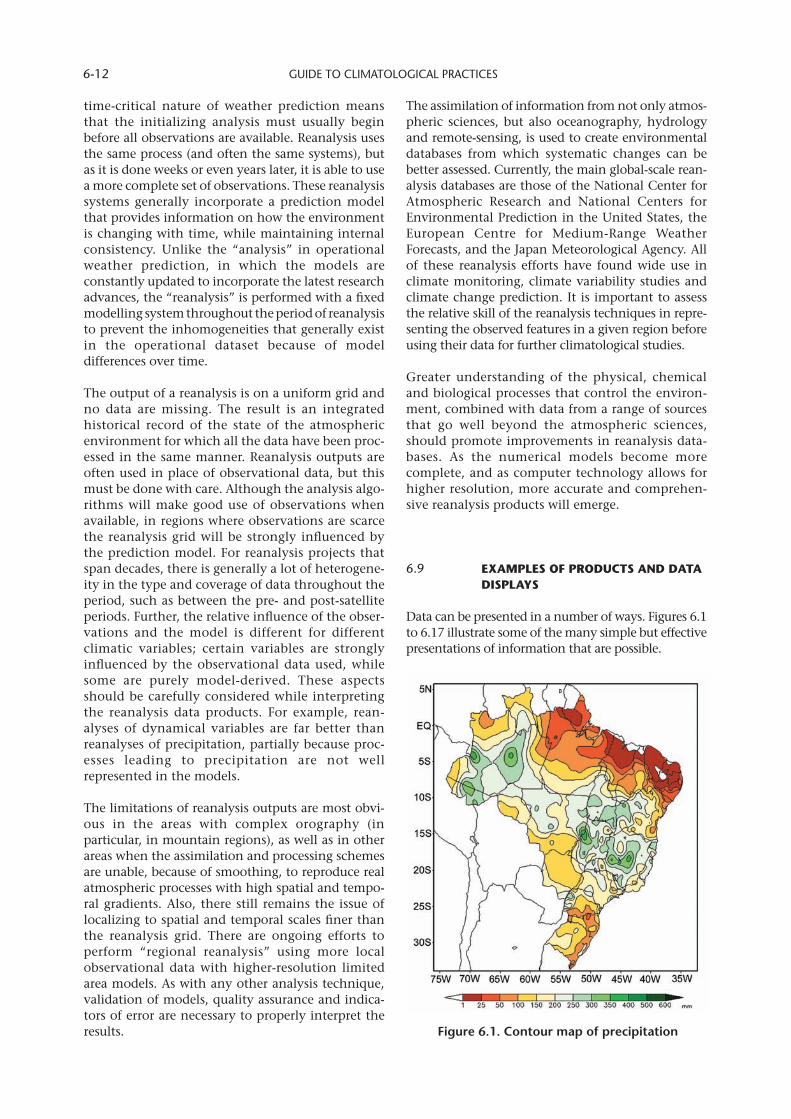
GUIDE TO CLIMATOLOGICAL PRACTICES 6-12
time-critical nature of weather prediction means that the initializing analysis must usually begin before all observations are available. Reanalysis uses the same process (and often the same systems), but as it is done weeks or even years later, it is able to use a more complete set of observations. These reanalysis systems generally incorporate a prediction model that provides information on how the environment is changing with time, while maintaining internal consistency. Unlike the “analysis” in operational weather prediction, in which the models are constantly updated to incorporate the latest research advances, the “reanalysis” is performed with a fixed modelling system throughout the period of reanalysis to prevent the inhomogeneities that generally exist in the operational dataset because of model differences over time.
The output of a reanalysis is on a uniform grid and no data are missing. The result is an integrated historical record of the state of the atmospheric environment for which all the data have been proc-essed in the same manner. Reanalysis outputs are often used in place of observational data, but this must be done with care. Although the analysis algo-rithms will make good use of observations when available, in regions where observations are scarce the reanalysis grid will be strongly influenced by the prediction model. For reanalysis projects that span decades, there is generally a lot of heterogene-ity in the type and coverage of data throughout the period, such as between the pre- and post-satellite periods. Further, the relative influence of the obser-vations and the model is different for different climatic variables; certain variables are strongly influenced by the observational data used, while some are purely model-derived. These aspects should be carefully considered while interpreting the reanalysis data products. For example, rean-alyses of dynamical variables are far better than reanalyses of precipitation, partially because proc-esses leading to precipitation are not well represented in the models.
The limitations of reanalysis outputs are most obvi-ous in the areas with complex orography (in particular, in mountain regions), as well as in other areas when the assimilation and processing schemes are unable, because of smoothing, to reproduce real atmospheric processes with high spatial and tempo-ral gradients. Also, there still remains the issue of localizing to spatial and temporal scales finer than the reanalysis grid. There are ongoing efforts to perform “regional reanalysis” using more local observational data with higher-resolution limited area models. As with any other analysis technique, validation of models, quality assurance and indica-tors of error are necessary to properly interpret the results.
The assimilation of information from not only atmos-pheric sciences, but also oceanography, hydrology and remote-sensing, is used to create environmental databases from which systematic changes can be better assessed. Currently, the main global-scale rean-alysis databases are those of the National Center for Atmospheric Research and National Centers for Environmental Prediction in the United States, the European Centre for Medium-Range Weather Forecasts, and the Japan Meteorological Agency. All of these reanalysis efforts have found wide use in climate monitoring, climate variability studies and climate change prediction. It is important to assess the relative skill of the reanalysis techniques in repre-senting the observed features in a given region before using their data for further climatological studies.
Greater understanding of the physical, chemical and biological processes that control the environ-ment, combined with data from a range of sources that go well beyond the atmospheric sciences, should promote improvements in reanalysis data-bases. As the numerical models become more complete, and as computer technology allows for higher resolution, more accurate and comprehen-sive reanalysis products will emerge.
6.9 EXAMPLESOFPRODUCTSANDDATADISPLAYS
Data can be presented in a number of ways. Figures 6.1 to 6.17 illustrate some of the many simple but effective presentations of information that are possible.
Figure.6 .1 ..Contour.map.of.precipitation
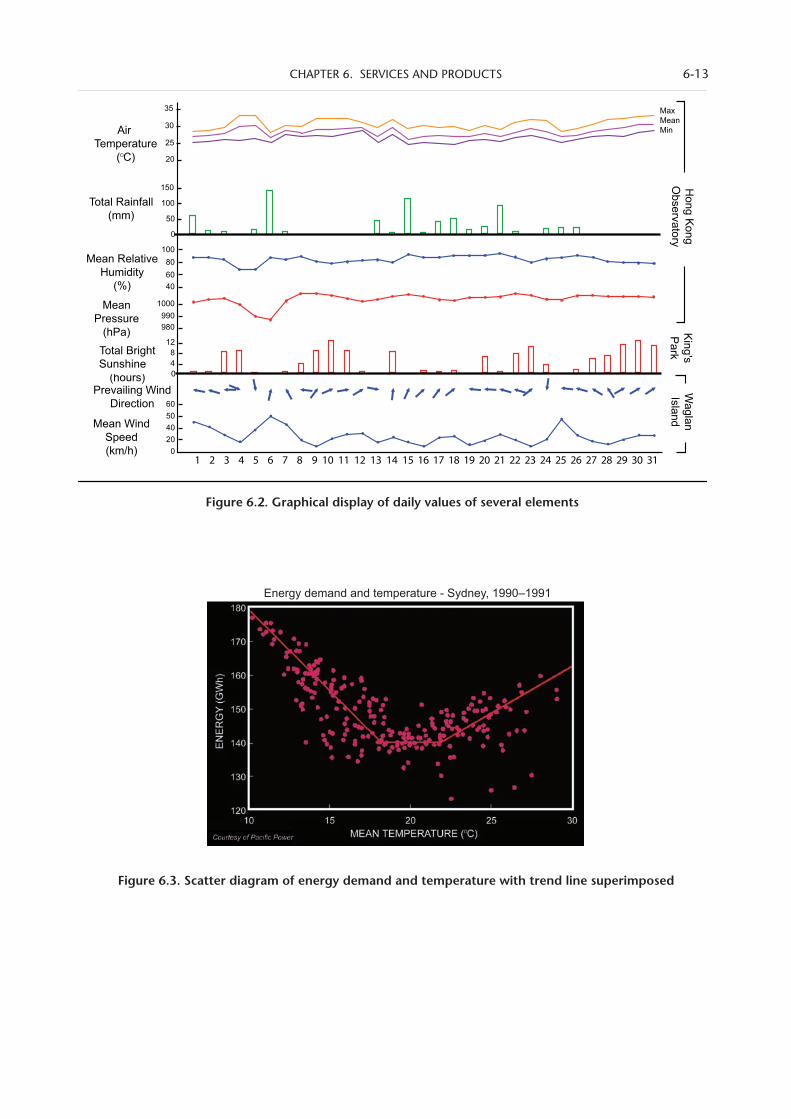
CHAPTER 6. SERVICES AND PRODUCTS 6-13
Sunshine
Figure.6 .2 ..Graphical.display.of.daily.values.of.several.elements.
Figure.6 .3 ..Scatter.diagram.of.energy.demand.and.temperature.with.trend.line.superimposed.
Energy demand and temperature - Sydney, 1990–1991
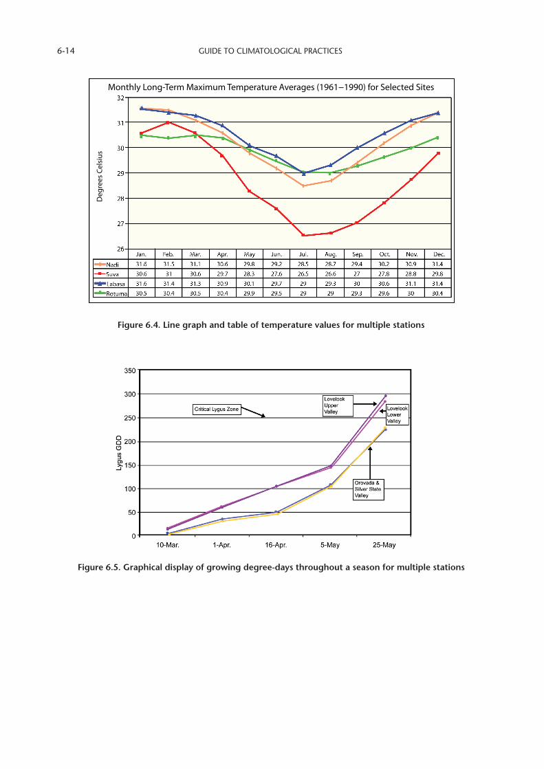
GUIDE TO CLIMATOLOGICAL PRACTICES 6-14
Figure 6.4. Line graph and table of temperature values for multiple stations
Monthly Long-Term Maximum Temperature Averages (1961−1990) for Selected SitesD
egre
es C
elsi
us
Figure 6.5. Graphical display of growing degree-days throughout a season for multiple stations
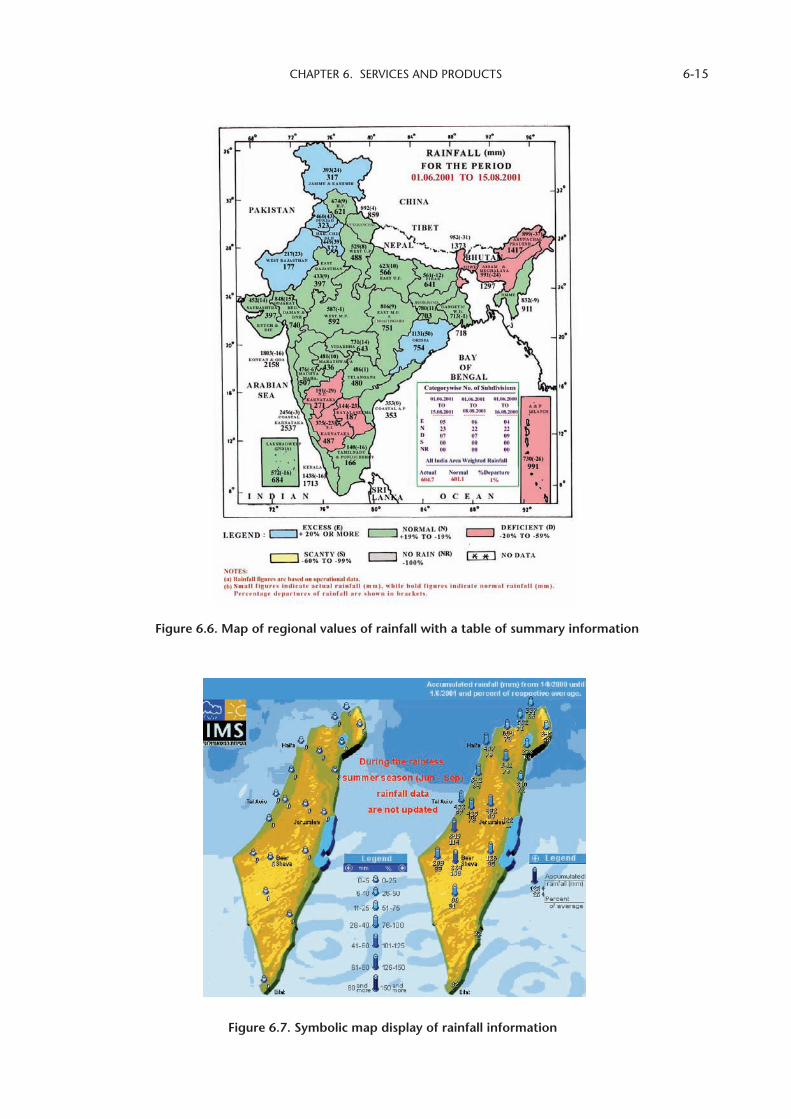
CHAPTER 6. SERVICES AND PRODUCTS 6-15
Figure.6 .6 ..Map.of.regional.values.of.rainfall.with.a.table.of.summary.information
Figure.6 .7 ..Symbolic.map.display.of.rainfall.information
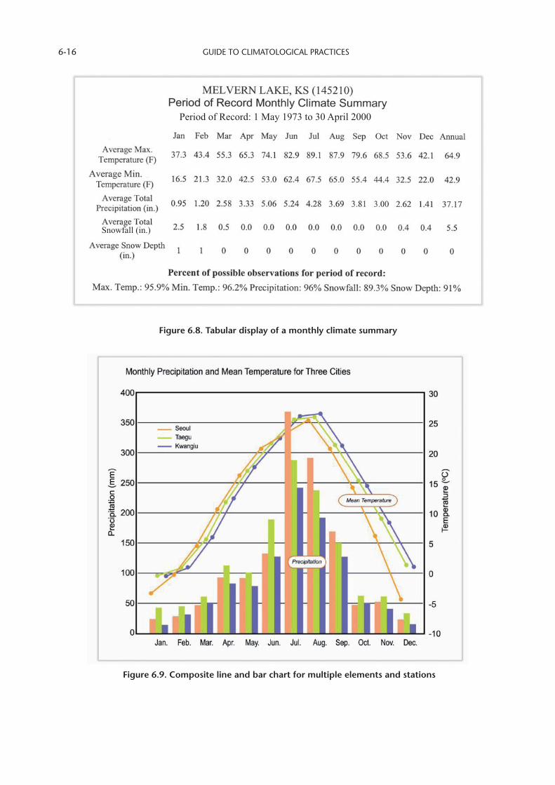
GUIDE TO CLIMATOLOGICAL PRACTICES 6-16
Figure.6 .8 ..Tabular.display.of.a.monthly.climate.summary
Period of Record: 1 May 1973 to 30 April 2000
T
Snowfall (in.)
Figure.6 .9 ..Composite.line.and.bar.chart.for.multiple.elements.and.stations
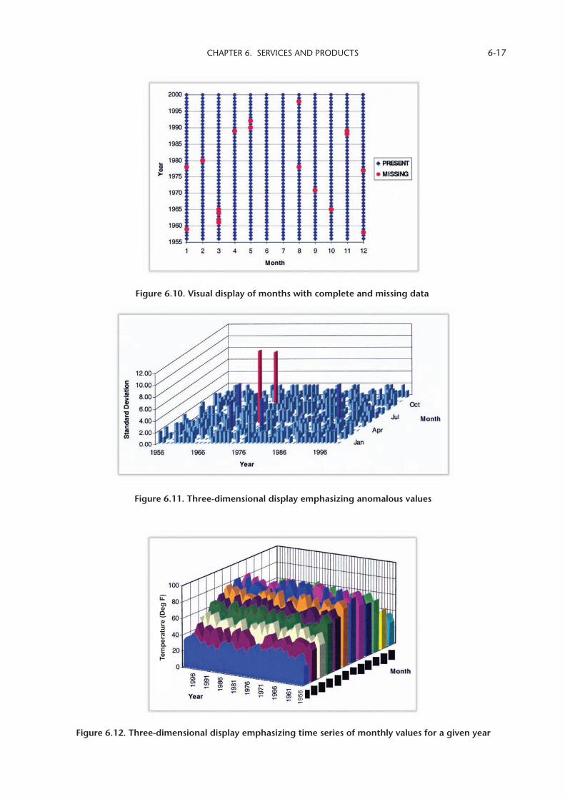
CHAPTER 6. SERVICES AND PRODUCTS 6-17
Figure.6 .10 ..Visual.display.of.months.with.complete.and.missing.data
Figure.6 .11 ..Three-dimensional.display.emphasizing.anomalous.values
Figure.6 .12 ..Three-dimensional.display.emphasizing.time.series.of.monthly.values.for.a.given.year
Tem
pera
ture
(Deg
F)
1956
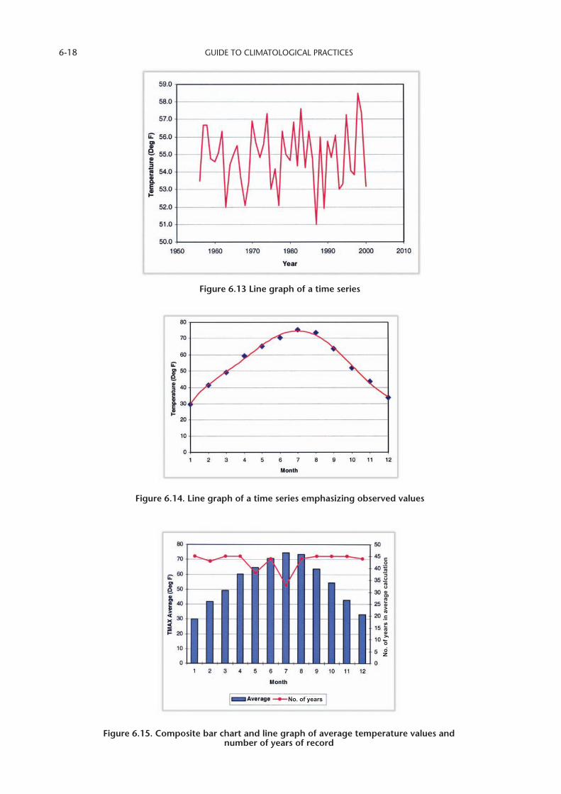
GUIDE TO CLIMATOLOGICAL PRACTICES 6-18
Figure.6 .13.Line.graph.of.a.time.series
Figure.6 .14 ..Line.graph.of.a.time.series.emphasizing.observed.values
Figure.6 .15 ..Composite.bar.chart.and.line.graph.of.average.temperature.values.and..number.of.years.of.record
No. of years
No.
of y
ears
in a
vera
ge c
alcu
latio
n
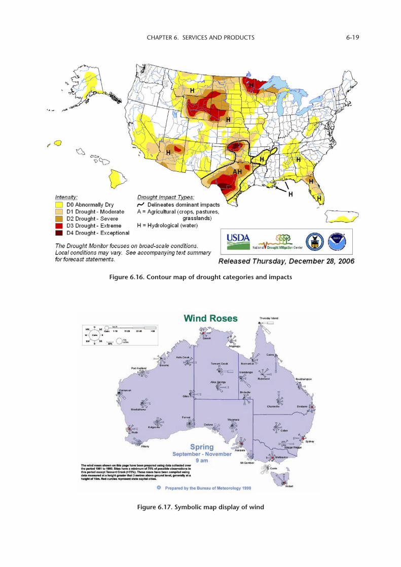
CHAPTER 6. SERVICES AND PRODUCTS 6-19
Figure.6 .17 ..Symbolic.map.display.of.wind
Figure.6 .16 ..Contour.map.of.drought.categories.and.impacts
GUIDE TO CLIMATOLOGICAL PRACTICES 6-20
6.10 REFERENCES
6.10.1 WMOpublications
World Meteorological Organization, 1983: Guide to Climatological Practices. Second edition (WMO-No. 100), Geneva.
———, 1988: Technical Regulations. Vol. I – General Meteorological Standards and Recommended Practices; Vol. II – Meteorological Service for International Air Navigation; Vol. III – Hydrology; Vol. IV – Quality Management (WMO-No. 49), Geneva.
———, 1991: Manual on the Global Data-processing System. Vol. I – Global Aspects. Supplement No. 10, October 2005 (WMO-No. 485), Geneva.
———, 1992: Manual on the Global Data-processing System. Vol. II – Regional Aspects. Supplement No. 2, August 2003 (WMO-No. 485), Geneva.
———, 1992: Operational Climatology - Climate Applications: On Operational Climate Services and Marketing, Information and Publicity: Report to the Eleventh Session of the Commission for Climatology (Havana, February 1993) (CCl Rapporteurs on Operational Climatology, J.M. Nicholls, and Marketing, Information and Publicity, D.W. Phillips). World Climate Applications and Services Programme (WMO/TD-No. 525, WCASP-No. 20), Geneva.
———, 1995: Hydrological Forecasts for Hydroelectric Power Production (WMO/TD-No. 118), Geneva.
———, 1995: Meeting of Experts on Climate Information and Prediction Services (CLIPS): Report of the Meeting (Melbourne, 28–31 March 1995) (WMO/TD-No. 680, WCASP-No. 32), Geneva.
———, 1996: Economic and Social Benefits of Climatological Information and Services: A Review of Existing Assessments (J.M. Nicholls) (WMO/TD- No. 780, WCASP-No. 38), Geneva.
———, 1996: Report of the Second Session of the CCI Working Group on Operational Use of Climatological Knowledge (Geneva, 28–31 May 1996) and Report of the Meeting of Experts on CLIPS (Geneva, 22–24 May 1996) (WMO/TD-No. 774, WCASP-No. 37), Geneva.
———, 1999: Report of the Planning Meeting for the Shanghai CLIPS Showcase Project: Heat/Health Warning System (Shanghai, 6–8 October 1999) (WMO/TD-No. 984, WCASP-No. 49), Geneva.
———, 2007: WMO Statement on the Status of the Global Climate in 2006 (WMO-No. 1016), Geneva.
———, 2008: Inter-Commission Task Team on the Quality Management Framework, Third Session, Final Report (Geneva, Switzerland, 28–30 October 2008), Geneva.
———, 2008: Report on the Activities of the Working Group on Climate Change Detection and Related Rapporteurs 1998–2001 (WMO/TD-No. 1071, WCDMP-No. 47), Geneva.
_________________________
6.10.2 Additionalreading
American Meteorological Society, 1993: Guidelines for using color to depict meteorological information. Bull. Amer. Meteor. Soc., 74:1709–1713.
Brohan, P., J.J. Kennedy, I. Harris, S.F.B. Tett and P.D. Jones, 2006: Uncertainty estimates in regional and global observed temperature changes: A new dataset from 1850. J. Geophys. Res., 111: D12106.
Hargreaves, G.H., 1975: Moisture availability and crop production. Trans. ASAE, 18:980–984.
Jones, P.D., M. New, D.E. Parker, S. Martin and I.G. Rigor, 1999: Surface air temperature and its variations over the last 150 years. Rev. Geophys., 37:173–199.
Khambete, N.N., 1992: Agroclimatic classification for assessment of the crop potential of Karnataka. Mausam, 43(1):91–98.
MacCracken, M., 2002: Do the uncertainty ranges in the IPCC and U.S. National Assessments account adequately for possibly overlooked climatic influences? Climatic Change , 52:13–23.
Palmer, W.C., 1965: Meteorological Drought. Weather Bureau Research Paper No. 45. Washington, DC, United States Department of Commerce.
Peterson, T.C., 2005: Climate change indices. WMO Bulletin, 54:83–86.
Peterson, T.C. and M.J. Manton, 2008: Monitoring changes in climate extremes: A tale of interna-tional cooperation. Bull. Amer. Meteor. Soc., 89:1266–1271.
Rayner, N.A., P. Brohan, D.E. Parker, C.K. Folland, J.J. Kennedy, M. Vanicek, T. Ansell and S.F.B. Tett, 2006: Improved analyses of changes and uncertainties in marine temperature measured in situ since the mid-nineteenth century: The HadSST2 dataset. J. Climate, 19:446–469.
Sarker, R.P. and B.C. Biswas, 1988: A new approach to agroclimatic classification to find out crop potential. Mausam, 39(4):343–358.
Tufte, E.R., 1990: Envisioning Information. Cheshire, Connecticut, Graphic Press.
United States Global Change Research Program Office (USGCRP), 2000: Climate Change Impacts on the United States: The Potential Consequences of Climate Variability and Change. Washington, DC, USGCRP.
Wang, B. and Z. Fan, 1999: Choice of South Asian summer monsoon indices. Bull. Amer. Meteor. Soc., 80:629–638.
Wilhelm, W.W., K. Ruwe and M.R. Schlemmer, 2000: Comparisons of three Leaf Area Index meters in a corn canopy. Crop Science, 40:1179–1183.
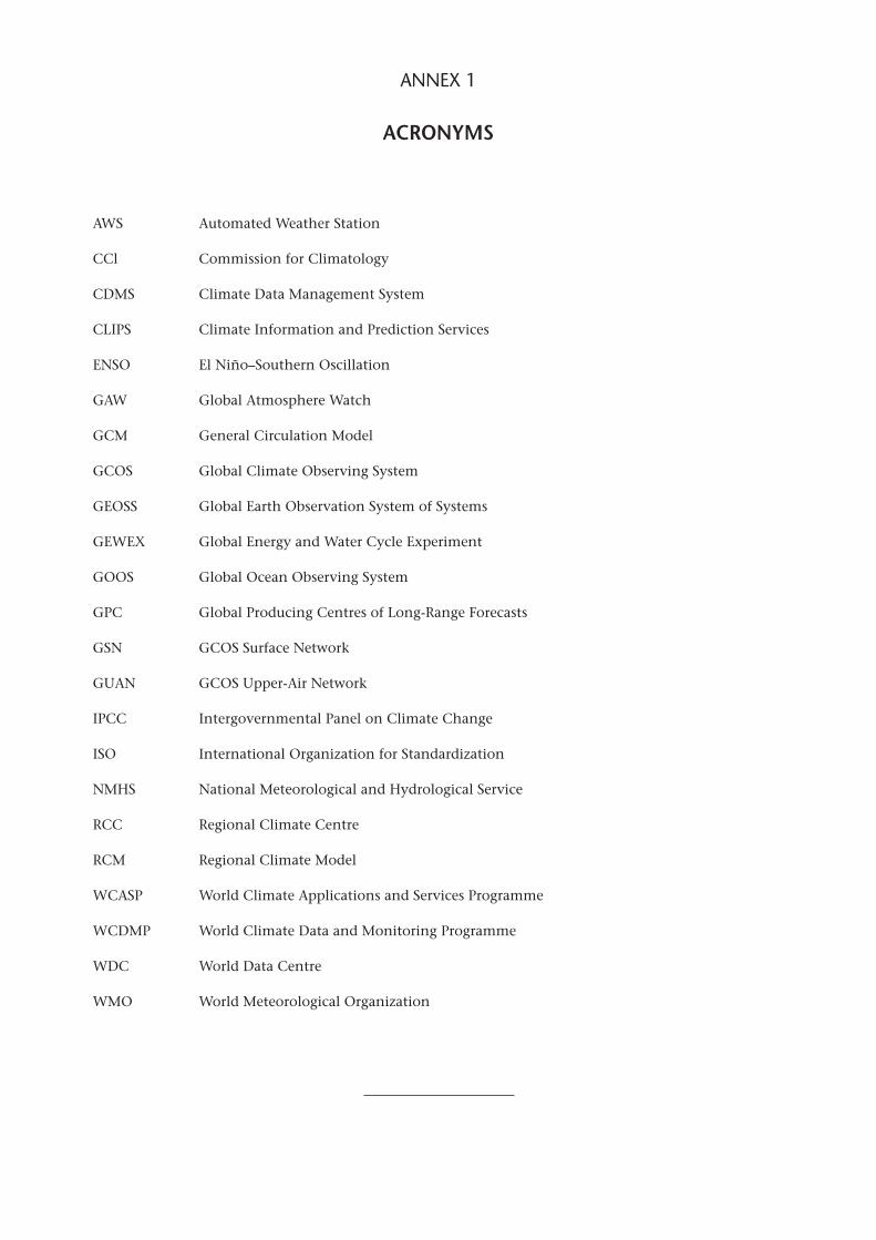
ANNEX 1
ACRONYMS
AWS Automated Weather Station
CCl Commission for Climatology
CDMS Climate Data Management System
CLIPS Climate Information and Prediction Services
ENSO El Niño–Southern Oscillation
GAW Global Atmosphere Watch
GCM General Circulation Model
GCOS Global Climate Observing System
GEOSS Global Earth Observation System of Systems
GEWEX Global Energy and Water Cycle Experiment
GOOS Global Ocean Observing System
GPC Global Producing Centres of Long-Range Forecasts
GSN GCOS Surface Network
GUAN GCOS Upper-Air Network
IPCC Intergovernmental Panel on Climate Change
ISO International Organization for Standardization
NMHS National Meteorological and Hydrological Service
RCC Regional Climate Centre
RCM Regional Climate Model
WCASP World Climate Applications and Services Programme
WCDMP World Climate Data and Monitoring Programme
WDC World Data Centre
WMO World Meteorological Organization
.
ANNEX 2
INTERNATIONAL.CLIMATE.ACTIVITIES
A2.1 COORDINATIONOFCLIMATEACTIVITIES
The Commission for Climatology is responsible for promoting and facilitating activities relating to climate and its relationship with human well-being, socio-economic activities, natural ecosystems and sustainable development. Specifically, it:(a) Coordinates and consolidates general require-
ments and standards for observations, data collection, archiving and data exchange for all components of the World Climate Programme;
(b) Identifies best practices in management of climate data, including near-real-time data, proxy data, remote-sensing data, and meta-data (information about data);
(c) Promotes dissemination of data, products and methods in support of research, applications, impact assessments and climate system moni-toring;
(d) Supports preparation of authoritative state-ments on climate, including the Annual State-ments on the Status of the Global Climate and regular El Niño and La Niña Updates;
(e) Evaluates and reviews development and appli-cation of operational climate predictions;
(f) Identifies priorities for studying the climates of natural and managed ecosystems and for providing climate information for alleviating problems arising from the influence of human activities on local and regional climate;
(g) Supports capacity-building and technology transfer;
(h) Promotes research and evaluation of the role of climate in key social and economic sectors in partnership with other WMO Technical Commissions, other United Nations agencies and relevant international and regional insti-tutions;
(i) Assesses the potential for application of seasonal prediction and other climatologi-cal services for social and economic benefit, including reduction of risk to climate-related hazards and optimal utilization of climate as a resource;
(j) Provides advice on issues relating to the access and availability of climatological data and services.
The Commission promotes and relies on a range of national, regional and global entities involved in climate-related matters. Apart from NMHSs, these entities include other United Nations agencies such
as the Food and Agriculture Organization of the United Nations; the World Health Organization; the United Nations World Tourism Organization; the United Nations Human Settlements Programme; the United Nations Environment Programme; the United Nations Development Programme; and the United Nations Educational, Scientific and Cultural Organization. The Commission for Climatology also works extensively with non-governmental organizations such as the International Federation of Red Cross and Red Crescent Societies, the International Council for Science, research institu-tions, universities, professional associations, academia, and development agencies such as the World Bank.
A2.2 THEWORLDCLIMATEPROGRAMME
In the 1970s it became obvious that greater interna-tional coordination and effort were needed to tackle the deficiencies in the understanding of climate and how to deal with the wide range of climatic influ-ences on society and the environment, some beneficial and others detrimental. In 1974 the Executive Council of the World Meteorological Organization agreed that WMO should initiate an international programme on climate and laid the foundations of the World Climate Programme. In 1978 the Economic and Social Council of the United Nations requested that WMO devote particular attention to those aspects of the Programme which would provide prompt and effective assistance to national planners and decision-makers in formulat-ing economic and social programmes and activities in their respective countries.
The First World Climate Conference in February 1979 recognized that the problem of possible human influence on climate was a matter of special importance. The Conference Declaration stressed the urgent need “for the nations of the world to take full advantage of man’s present knowledge of climate; to take steps to improve significantly that knowledge; and to foresee and to prevent potential man-made changes in climate that might be adverse to the well-being of humanity”.
The eighth World Meteorological Congress formally created the World Climate Programme in 1979, recognizing that the cooperation of many other United Nations agencies and other international organizations was needed to support the
GUIDE TO CLIMATOLOGICAL PRACTICES Ann–2
programme. Responsibility for the overall coordi-nation of the programme and for climate data and applications was assumed by WMO, while the United Nations Environment Programme assumed responsibility for climate impact studies, and WMO together with the International Council for Science agreed to jointly implement the climate research programme. The structure of the World Climate Programme and the partners cooperating with WMO have evolved over time.
There are four main components of the World Climate Programme. The World Climate Data and Monitoring Programme (WCDMP) facilitates the effective collection and management of climate data and the monitoring of the global climate system, including the detection of climate variability and change. The World Climate Applications and Services Programme (WCASP) fosters scientific understanding of the role of climate in human activities, effective application of climate knowledge and information for the benefit of society, tailored climate services for users in various socioeconomic sectors, and the prediction of significant climate variations (both natural and as a result of human activity). The Climate Information and Prediction Services (CLIPS) project was established by WMO as an implementation arm of WCASP. The World Climate Impact Assessment and Response Strategies Programme, implemented by the United Nations Environment Programme, assesses the impacts of climate variability and changes that could markedly affect economic or social activities and advises governments on these matters; it also contributes to the develop-ment of a range of socio-economic response strategies that could be used by governments and communities. The World Climate Research Programme (WCRP), jointly sponsored by WMO, the International Council for Science and the Intergovernmental Oceanographic Commission of the United Nations Educational, Scientific and Cultural Organization, seeks to improve the basic scientific understanding of climate processes for determining the predictability of climate, climate variability and change, and the extent of human influence on climate, and for developing the capability for climate prediction. The activities and projects of WCRP include studies of the dynamics and thermodynamics of the Earth’s atmosphere, the atmosphere’s interactions with the Earth’s surface, and the global water cycle; climate variability and predictability; interaction of dynamical, radiative and chemical processes; processes by which the cryosphere interacts with the rest of the climate system; and biogeochemi-cal and physical interactions between the ocean and the atmosphere.
The Second World Climate Conference in 1990 recognized an urgent need to acquire comprehen-sive information on the properties and evolution of the Earth’s climate system, to detect climate change, to support climatological applications for economic development, and to develop climate science and predictions. The Eleventh World Meteorological Congress in 1991 decided that a global climate observing system should be established. This system would be based on the coordination and associa-tion of existing or planned operational and research programmes for observing the global environment and on the further development of those programmes required to ensure continuity of infor-mation over decades.
In 1992, the Global Climate Observing System (GCOS) was formally established under a Memorandum of Understanding among WMO, the Intergovernmental Oceanographic Commission of the United Nations Educational, Scientific and Cultural Organization, the United Nations Environment Programme, and the International Council for Science. While GCOS does not directly make observations or generate data products, it works closely with and builds upon existing and developing observing systems and provides a frame-work for integrating the systems of participating countries and organizations. The systems and networks included are:(a) GCOS Surface Network (GSN) and Upper-Air
Network (GUAN) (subsets of the WMO World Weather Watch Global Observing System);
(b) WMO Global Atmosphere Watch (GAW);(c) WCRP/GEWEX Baseline Surface Radiation
Network; (d) Global Ocean Observing System (GOOS),
including ocean observing systems such as the Global Sea Level Observing System;
(e) Global Terrestrial Observing System, includ-ing the Global Terrestrial Network for Glaciers and the Global Terrestrial Network for Perma-frost;
(f) World Hydrological Cycle Observing System.
The concept of coordinated and comprehensive Earth observations was promoted at the First Earth Observation Summit in 2003. At the Third Earth Observation Summit held in 2005, the Global Earth Observation System of Systems (GEOSS) was formally established to build on, and add value to, existing national, regional and international observation systems by coordinating efforts, addressing critical gaps, supporting interoperabil-ity, sharing information, reaching a common understanding of user requirements, and improv-ing delivery of information to users. GEOSS supports GCOS by expanding on the range of climate-related variables identified in the GCOS
ANNEX 2. INTERNATIONAL CLIMATE ACTIVITIES Ann–3
Implementation Plan and by assisting the parties in meeting their responsibilities under the United Nations Framework Convention on Climate Change (see section A2.4).
A2.3 THECLIMATEAGENDA
In the early 1990s, development of increasingly close collaboration among climate-related programmes of a number of international organi-zations led to the establishment by WMO of the Coordinating Committee for the World Climate Programme. In 1995 a draft interagency document entitled The Climate Agenda – International Climate-Related Programmes: A Proposal for an Integrating Framework was issued. The four main thrusts were new frontiers in climate science and prediction, climate services for sustainable development, dedicated observations of the climate system, and studies of climate impact assessments and response strategies to reduce vulnerability. The leaders of these thrusts were WMO, the Food and Agriculture Organization of the United Nations and the United Nations Environment Programme.
The Twelfth World Meteorological Congress endorsed the Climate Agenda in 1995 and estab-lished an Interagency Committee on the Climate Agenda. While the Committee provided some initial guidance, the fast pace of developments in climate-related matters led WMO at the 2001 session of its Executive Council to begin a process of considering new mechanisms for climate coordi-nation. At its sixty-first session in 2009, the WMO Executive Council agreed not to revitalize the Interagency Committee on the Climate Agenda, but to use the United Nations Delivering as One initiative to coordinate climate issues at the United Nations level.
A2.4 INTERNATIONALCLIMATECHANGEPROGRAMMES
At the First World Climate Conference in 1979, the international climate community expressed concern that “continued expansion of man’s activities on Earth may cause significant extended regional and even global changes of climate”, and called for global cooperation to “explore the possi-ble future course of global climate and to take this new understanding into account in planning for the future development of human society”. At a climate conference in Villach, Austria, in 1985 scientists from 29 developed and developing coun-tries concluded that the increasing concentrations of greenhouse gases were expected to cause a
significant warming of the global climate in the next century, as detailed in the Report of the International Conference on the Assessment of the Role of Carbon Dioxide and of Other Greenhouse Gases in Climate Variations and Associated Impacts (WMO-No. 661). They also noted that past climate data may no longer be a reliable guide for long-term projects because of expected warming of the global climate, that climate change and sea level rises are closely linked with other major environmental issues, that some warming appears inevitable because of past activities, and that the future rate and degree of warming could be profoundly affected by policies on emissions of greenhouse gases. Responding to these concerns, the United Nations Environment Programme, WMO and the International Council for Science established an Advisory Group on Greenhouse Gases in 1986 to ensure periodic assessments of the state of scien-tific knowledge on climate change and its implications.
In 1987 the Tenth World Meteorological Congress recognized the need for objective, balanced and internationally coordinated scientific assessment of the understanding of the effects of increasing concentrations of greenhouse gases on the Earth’s climate and the ways in which these changes may influence social and economic patterns. The United Nations Environment Programme and WMO agreed on an intergovernmental mechanism to provide scientific assessments of climate change, and in 1988 the WMO Executive Council, with support from the United Nations Environment Programme, estab-lished the Intergovernmental Panel on Climate Change to consider the need for: (a) Identification of uncertainties and gaps in
our present knowledge with regard to climate change and its potential impacts, and prepa-ration of a plan of action over the short term to fill these gaps;
(b) Identification of information needed to evalu-ate policy implications of climate change and response strategies;
(c) Review of current and planned national and international policies related to the green-house gas issue;
(d) Scientific and environmental assessments of all aspects of the greenhouse gas issue and the transfer of these assessments and other rele-vant information to governments and inter-governmental organizations, to allow them to be taken into account in policies on social and economic development and environmental programmes.
In November 1988 the IPCC established working groups to prepare assessment reports on the available scientific information on climate change (Working Group I), on environmental, social and economic
GUIDE TO CLIMATOLOGICAL PRACTICES Ann–4
of America, is testimony to the remarkable success of the IPCC process in informing the policymakers as well as the general public on the scientific underpin-nings of the climate change issue.
A2.5 REFERENCESANDADDITIONALREADING
Group on Earth Observations (GEO), 2005: Global Earth Observation System of Systems (GEOSS): 10-year Implementation Plan. Reference Document GEO 1000R/ESA SP-1284. Noordwijk, European Space Agency Publications Division, ESTEC.
———, 2007: GEO 2007–2009 Work Plan. Toward Convergence, Geneva.
Intergovernmental Panel on Climate Change (IPCC), 2007: The Fourth Assessment Report: Climate Change 2007 (AR4), Vols. 1–4. Cambridge, Cambridge University Press.
United Nations System Chief Executives Board for Coordination, 2008: Acting on Climate Change: The UN System Delivering as One, New York.
World Meteorological Organization, 1986: Report of the International Conference on the Assessment of the Role of Carbon Dioxide and of Other Greenhouse Gases in Climate Variations and Associated Impacts, (Villach, Austria, 9–15 October 1985) (WMO-No. 661), Geneva.
impacts of climate change (Working Group II), and on formulation of response strategies (Working Group III). The forty-third session of the United Nations General Assembly in 1988 endorsed the action of WMO and the United Nations Environment Programme to establish the IPCC and requested “a comprehensive review and recommendations with respect to, inter alia, the state of knowledge of the science of climate and climatic change; programmes and studies on the social and economic impact of climate change, including global warming; and possi-ble response strategies to delay, limit, or mitigate the impacts of adverse climate change”.
The IPCC adopted its first assessment report on 30 August 1990. Its findings, coupled with the outcomes of the Second World Climate Conference that same year, spurred governments to create the United Nations Framework Convention on Climate Change in March 1994. The IPCC Second Assessment Report was completed in late 1995, the third in 2001, and the fourth in 2007. The reports issued by the IPCC are frequently used to inform decisions made under the Framework Convention. They also played a major role in the negotiations leading to the Kyoto Protocol, a February 2005 international treaty that builds on the Framework Convention and sets legally binding targets and timetables for reducing the greenhouse gas emissions of industrialized countries. The award of the 2007 Nobel Peace Prize to the IPCC, along with Mr Al Gore, Former Vice-President of the United States
.


2011 edition
www.wmo.int
Guide to Climatological Practices
WMO-No. 100
GU
IDE
TO
CLI
MA
TO
LOG
ICA
L P
RA
CT
ICE
SW
MO
-No
. 100
P-C
LW_1
0126
4