
Class 4: Analysis of univariate data: measures of...
26
Statistics Class 4: Analysis of univariate data: measures of location of a data set Recommended reading: To really confuse yourself, look at how the Wikipedia defines percentiles .
Transcript of Class 4: Analysis of univariate data: measures of...
Statistics
Class 4: Analysis of univariate data: measures of location of a data set
Recommended reading:
To really confuse yourself, look at how the
Wikipedia defines percentiles.

Statistics
Measures of location
There are three standard measures of location of a sample data set.
• Mode
• Median
• Mean
These measures are used to represent typical, central or average values.
Other points of location are also of interest to represent more extreme values.
• Minimum
• Maximum
• Quartiles and Percentiles
Statistics
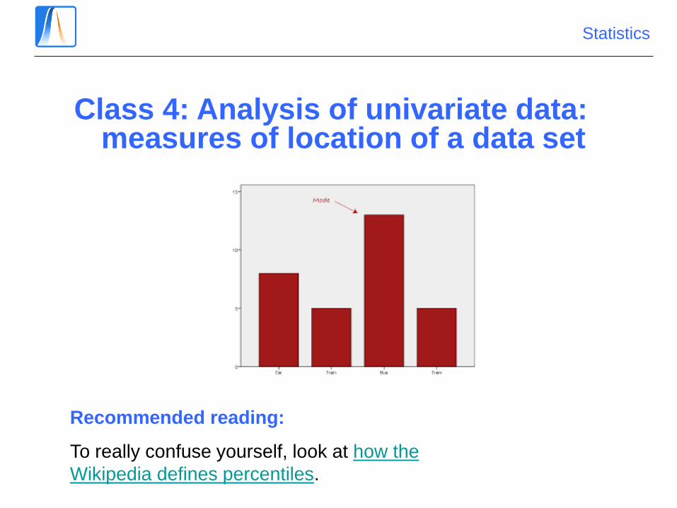
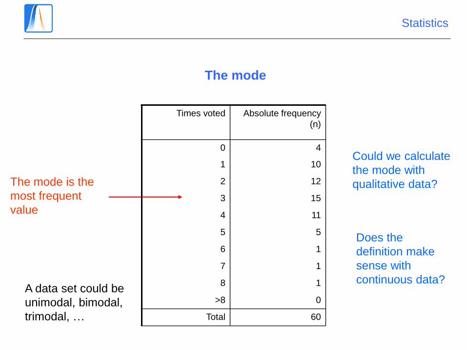
The mode
The mode is the
most frequent
value
A data set could be
unimodal, bimodal,
trimodal, …
Could we calculate
the mode with
qualitative data?
Does the
definition make
sense with
continuous data?
Times voted Absolute frequency
(n)
0 4
1 10
2 12
3 15
4 11
5 5
6 1
7 1
8 1
>8 0
Total 60

Statistics
The mode with continuous data
We have a modal Interval
What would we do if the classes were of
different widths?

Statistics
An exact value for the mode with grouped data
The mode is at the centre of the
modal Interval.
What about
different width
intervals?

Statistics
The mode with intervals of different width
For an alternative point estimate of the mode, see this page.

Statistics
The median
The median is the most central observation:
5 3 11 21 7 5 2 1 3
What is the median?
Would it make a difference if N was odd or even?
Could we calculate the
median with qualitative
data?

Statistics
The median is ½*(3+3)=3
Times voted
3 3 3 4 1 2 4 5 2 3 1 1 3 8 4 1 3 4 2 5 0 0 5 4 2 1 2 3 3 2
1 4 3 2 3 5 0 6 3 1 3 5 4 1 4 1 2 4 4 3 3 0 7 2 2 1 3 4 2 2
0 0 0 0 1 1 1 1 1 1 1 1 1 1 2 2 2 2 2 2 2 2 2 2 2 2 3 3 3 3
3 3 3 3 3 3 3 3 3 3 3 4 4 4 4 4 4 4 4 4 4 4 5 5 5 5 5 6 7 8

Statistics
Median
< 0,5
≥ 0,5
Calculating the median from the frequency table (discrete data)

Statistics
The median with grouped data
Spending ni
Ni
fi
Fi
≤ 30 0 0 0 0
(30,45] 2 2 0,05555556 0,05555556
(45,60] 9 11 0,25 0,30555556
(60,75] 9 20 0,25 0,55555556
(75,90] 10 30 0,27777778 0,83333333
(90,105] 3 33 0,08333333 0,91666667
(105,120] 3 36 0,08333333 1
> 120 0 36 0 1
Total 36 1
Median interval
For a point estimate of the median, see this page.

Statistics
The mean
The mean (or arithmetic mean) is the average of the data.
For the case of the number of times voted, the mean is:
(3 + 3 + … + 2 + 2)/60 = 2.817
Can we calculate the mean
for qualitatve data?

Statistics
Calculating the mean from the frequency table (discrete data)
Times
voted (x)
Absolute
frequency (n)
Relative
frequency (f)n x f x
0 4 0,07 0 0,00
1 10 0,17 10 0,17
2 12 0,20 24 0,40
3 15 0,25 45 0,75
4 11 0,18 44 0,73
5 5 0,08 25 0,42
6 1 0,02 6 0,10
7 1 0,02 7 0,12
8 1 0,02 8 0,13
>8 0 0,00 0 0,00
Total 60 1,00 169 2,82
169/60 = 2,82

Statistics
The mean with grouped data
This is an approximation using the centre of each Interval as the
marca de clase.
Yearly
spending (€)
Centre
(x)
Absolute
frequency (n)
Relative
frequency (f)x f
≤ 30 22,5 0 0,00 0,00
(30,45] 37,5 2 0,06 2,08
(45,60] 52,5 9 0,25 13,13
(60,75] 67,5 9 0,25 16,88
(75,90] 82,5 10 0,28 22,92
(90,105] 97,5 3 0,08 8,13
(105,120] 112,5 3 0,08 9,38
> 120 127,5 0 0,00 0,00
Total 36 1,00 72,5

Statistics
Sensitivity of the mean to outlying data
1 2 2 3 3 3 3 4 4 5
Mode = median = mean = 3
1 2 2 3 3 3 3 4 4 500
Mode = median = 3, mean = 52.5
The mean is very sensitive to extreme or outlying data!

Statistics
The mode, median and mean with skewed data
Which is which?
What would the values
be with a symmetrical
sample?
Data very
skewed to the
right.

Statistics
Other points of the distribution: minimum, maximum.
We are not always interested in just measures of central location.
Often it is more interesting to look at the most extreme data.
0 0 0 0 1 1 1 1 1 1 1 1 1 1 2 2 2 2 2 2 2 2 2 2 2 2 3 3 3 3
3 3 3 3 3 3 3 3 3 3 3 4 4 4 4 4 4 4 4 4 4 4 5 5 5 5 5 6 7 8
Minimum = 0
Maximum = 8Next week, we’ll see how
to check if these data are
“strange” or outlying.

Statistics
Other points of the distribution: percentiles.
The idea of the median is to find a point to separate the data into two
halves. We could generalise this by trying to separate into parts of size p
and 1-p.
The point that does this is called the p x 100% percentile.
How can we calculate this?
5 3 11 21 7 5 2 1 3
• Before we do anything, we have to order the data.
1 2 3 3 5 5 7 11 21

Statistics
Other points of the distribution: percentiles.
• Now calculate r = p x (N + 1) where N is the sample size.
1 2 3 3 5 5 7 11 21
Suppose we want the 80% percentile.
r= 0.8 x (9 + 1) = 8.
What if we want the 66.67% percentile?
r= 2/3 x (9+1) = 6.67.

Statistics
Other points of the distribution: percentiles.
• If r is a whole number, then the percentile is the r’th point of the ordered
data set.
1 2 3 3 5 5 7 11 21
Suppose we want the 80% percentile.
r = 0.8 x (9 + 1) = 8.
The 80% percentile is equal to 11.
Statistics
Other points of the distribution: percentiles.
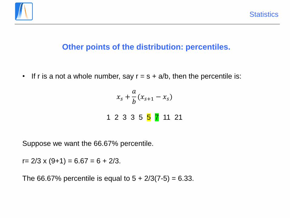
• If r is a not a whole number, say r = s + a/b, then the percentile is:
𝑥𝑠 +𝑎
𝑏(𝑥𝑠+1 − 𝑥𝑠)
1 2 3 3 5 5 7 11 21
Suppose we want the 66.67% percentile.
r= 2/3 x (9+1) = 6.67 = 6 + 2/3.
The 66.67% percentile is equal to 5 + 2/3(7-5) = 6.33.

Statistics
Other points of the distribution: quartiles.
The 25% and 75% percentiles are called the first and third quartiles.
1 2 3 3 5 5 7 11 21
r = ¼ x (9 + 1) = 2.5
The first quartile is 2 + ½ (3-2) = 2.5.
What is the third quartile?
The minimum is the 0th quartile, the median the second quartile and the
maximum the 4th quartile.

Statistics
What is the 80%
percentile?
Calculating percentiles from the frequency table (discrete data)

Statistics
Exercise
The following table represents the ages of 10 PP mayors in the Community of
Madrid.
40 40 35 50 50 40 40 60 50 35
Mark the correct response among the following:
a) The mode and median are 40 and the mean is 44.
b) The mode and mean are 40 and the median 44.
c) The mean and median are 40 and the mode is 44.
d) None of the above.

Statistics
Ejercicio (Test 1 2008-2009)
Certain politicians are well known for letting their speeches go on a long time.
The following chart records the lengths of some of the last political speeches (in
minutes) of a very well known politician (FC).
Time ni fi
(0-30] 6 0.18
(30-60] 13 0.38
(60-90] 13 0.38
(90-120] 2 0.06
Total 34 1
Estimate the average speech length.

Statistics
Exercise
The table below shows the gender and age of various Ministers in the Zapatero
government.
• What is the modal class of the gender of the ministers?
• Calculate the mode, median and mean age of the ministers.
• Estimate the third quartile of the ages of the ministers.
Name Gender Ministry Age
Bibiana Aído F Igualdad 33
Carme Chacón F Defensa 38
Ángeles González-Sinde F Cultura 44
Cristina Garmendia F Ciencia e innovación 47
Trinidad Jiménez F Sanidad y Política Social 47
José Blanco M Fomento 48
Ángel Gabilondo M Educación 60
Elena Salgado F Economía y Hacienda 60


![Regresión y modelos lineales [5mm] [height=1.5in]../Images ...halweb.uc3m.es/esp/Personal/personas/mwiper/docencia/Spanish/In… · Regresión y modelos lineales Mike Wiper Departamento](https://static.fdocuments.in/doc/165x107/5eae3f8de60e9147df477ca5/regresin-y-modelos-lineales-5mm-height15inimages-regresin-y-modelos.jpg)
