1

Chilean Unremunerated Reserve Requirement Capital Controls as a Screening Mechanism

Abstract This paper presents a model of Chilean style “speed bump” capital controls that interprets them as a mechanism for screening out volatile investor types. This interpretation is contrasted with a public finance explanation which views speed bumps as a tax on short term capital inflows that raises their relative price. A surprising result is that even though speed bumps raise the cost of capital, they may actually increase the level of inflows. These increased inflows are more stable because they are provided by patient investors. The lesson is that screening out volatile investor types stabilizes the financial environment. Speed bumps benefit both firms and patient investors by reducing the damage done by sudden exit, which increases the demand for and supply of capital. Keywords: Speed bumps, capital controls, short term debt, screening mechanism. JEL ref.: F3.

Thomas I. Palley Director, Globalization Reform Project

Open Society Institute Washington, DC 20036

e-mail: tpalley@osi-dc.org

2

I Introduction

In the wake of the financial crises of the 1990s there has been much debate about how to

stabilize global financial markets. One policy suggestion that has been received well by both

progressives (Blecker, 1999; Grabel, 2002/03; Palley, 1999) and the mainstream (Council on

Foreign Relations, 1999; Eichengreen, 1999) is that of Chilean-style “speed bumps.”1 Thus far,

the case for speed bumps has been made largely on the basis of the twin empirical observations

that short term debt was a significant factor precipitating the east Asian financial crisis, and that

Chile has been able to tilt the composition of its inflows toward less risky longer-term capital.

The current paper provides a theoretical analysis of speed bumps that validates this empirical

case. The analysis is in terms of imperfect information, and has speed bumps serving as a

mechanism for screening “good/patient” and “bad/impatient” investors. This approach fits

squarely with the work of Nobel economist Joseph Stiglitz, who has been a prominent and vocal

critic of the IMF and its approach to the financial architecture.

Speed bumps are a form of temporarily applied capital control aimed at discouraging inflows

of short-term capital. They can be contrasted with traditional capital controls, such as imposed by

Malaysia in 1998, which are aimed at preventing outflows of capital. Speed bumps can embody a

number of different features including (i) a requirement that capital in-flows stay for a given

duration (in Chile’s case it was twelve months), (ii) placement of a temporary non-interest

bearing reserve requirement on all capital inflows that is refunded after a specified period, and

(iii) payment of a penalty in the event that a capital inflow reverses within a given period.

The paper examines the underlying microeconomic workings of Chilean-style speed bumps

and advances a new theory that emphasizes their role as a screening device. This approach

contrasts with the standard public finance approach which describes them as a tax on short term

flows. The public finance approach argues that speed bumps lower the relative return to short- 1. Paradoxically, just as opinion is converging on the benefits of speed bumps as an institution for tempering inflows of volatile short term capital, Chile is committed to eliminating them. “Investors to Watch Chile’s Presidential Election as Candidates Pledge to Kill Controls on Capital,” Wall Street Journal, 10 January, 2000.

3

term capital inflows, thereby discouraging such inflows. The screening approach maintains that

speed bumps asymmetrically impact investors with a proclivity to short term flight (i.e. investors

who are impatient or by driven herd instincts), which changes the composition of capital flows

into the country. The model that is developed comes up with the surprising result that though

speed bumps raise the cost of short term capital, they may also increase inflows of capital.

Moreover, these increased inflows are more stable since the composition of inflows is shifted

toward patient investors. This investor composition effect may explain why Chile managed to

avoid a financial market contagion effect in the wake of the east Asian and Brazilian financial

crises. Both of these analytical conclusions are supportive of speculations made by Grabel

(2002/03) that speed - bump type capital controls could actually lower hurdle rates of return in

developing countries.

II The public finance approach to speed bumps

The standard approach to explaining the effects of speed bumps emphasizes traditional public

finance concerns. Speed bumps effectively impose a tax on short term capital inflows, thereby

lowering the rate of return on such flows. Foreign investors therefore reduce their demand for

short term liabilities and total inflows fall.

This effect is captured in the following simple model. Borrowers’ demand for short term

foreign loans is a negative function of the short term interest rate, and is given by

(1) D = D( r,....) Dr < 0

where D = domestic borrowers’ demand for short term foreign borrowing, r = interest rate on

short term foreign borrowing. Financial markets are open to inflows of foreign capital, and

foreign lenders view loans to domestic borrowers as a perfect substitute with other international

lending. Consequently, foreign supply of loans is perfectly elastic at the going world interest

rate, and given by

(2) r = r*

4

where r* = world short term interest rate.2where e = expected rate of exchange rate appreciation

and p = country risk premium. Assuming a positive equilibrium in-flow of short term foreign

capital, this implies that the equilibrium short term interest rate is equal to r*. The equilibrium

quantity of foreign short term lending is

(4) D = D( r*, .....) Dr* < 0

Now suppose that the monetary authority imposes a k percent reserve requirement on all

short term capital inflows. In this event the return to foreign short term lenders adjusts such that

(5) [1 - k]r = r*

where k = reserve requirement ratio. The non-interest bearing reserve requirement means that

foreign investors only earn interest on [1 - k] of each dollar loaned, and the interest rate must rise

to compensate them so that their return equals that available in global financial markets. The

equilibrium interest rate and level of short term foreign borrowing are then given by

(6.a) r = r*/[1 - k]

(6.b) D = D(r*/[1 - k], ...)

The equilibria with and without the reserve requirement are shown in figure 1. Initially

there is total borrowing of D0. The interest rate is r*. Introduction of the reserve requirement

shifts the perfectly elastic foreign demand for short term liabilities up, and raises the equilibrium

interest rate to r*/[1-k]. Total short term borrowing falls to D1. This outcome is consistent with

the claim that speed bumps decrease short term inflows.

Since the price of long term capital is also set in world markets and is unaffected by the

introduction of speed bumps, the volume of long term inflows remains unchanged. Putting the

pieces together, total inflows therefore fall but the proportion of long term inflows rises.

III Speed bumps as a screening device: the case where borrowers are negatively impacted

by sudden withdrawals

2. Equation (3) assumes perfect substitutes and no exchange rate risk. If these assumptions do not hold, then the relationship becomes r = r* + e + p

5

The traditional public finance approach to speed bumps focuses on discouraging short term

borrowing by raising its relative cost. In the background there is a belief that short term

borrowing is deleterious, and therefore ought to be discouraged. This section presents an

alternative interpretation of speed bumps which views them as a screening mechanism. The

model focuses on the total level of inflows, emphasizing the damage done to investors by sudden

exits of capital. It describes how speed bumps can help screen out capital flows from sources

which are prone to flight, and this improves the stability and quality of capital inflows.

Consequently, there can even be an increase in total inflows as the reduction in damage done by

capital flight of unstable investors raises returns to stable investors who then become willing to

provide lend more.

Suppose there are two types of foreign investor consisting of patient investors (type A) and

impatient investors (type B). Investors know which type they are, but borrowers cannot observe

the type from which they are borrowing. The proportion of patient type A investors is x, and the

proportion of impatient type B investors is [1 - x], where 1 > x > 0. Patient investors invest in

countries on the basis of fundamentals and for the long haul, and therefore have a relatively low

probability (qA) of withdrawing their money in the short term (i.e. next twelve months).

Impatient investors are subject to investment fads and fashions, and have a relatively higher

probability (qB) of withdrawing their funds in the short term. Thus, qB > qA where 1 > qB > qA >

0. For simplicity, the probabilities of withdrawal across investor types are assumed to be

independent. Foreign investors can earn an expected return of r* on international capital markets.

Finally, in the event that an investor withdraws their funds, this imposes a cost of c per dollar on

the domestic borrower.3 3. This cost can be thought of as a composite cost that includes both internal and external components. One effect is that sudden withdrawals cause the price of short term issues to fall which raises interest rates and contributes to greater variability of interest rates, thereby raising firms’ ex-ante costs of financing. It can also be associated with a depreciation of the exchange rate which raises the burden of foreign currency denominated debt. This hurts individual borrowers, and also hurts the macro economy by causing a shortage of aggregate demand and reducing the value of collateral to back foreign borrowing needed to finance investment.

6

Under such conditions, speed bumps can be used to improve economic outcomes. This can

be seen by comparing the equilibrium outcome when there are no speed bumps with the outcome

when there are speed bumps.

Case I: no speed bumps. In the case where there are no speed bumps, borrowers are unable to

distinguish between lender types. The result is a pooled equilibrium in which all foreign lenders

are paid the same rate of return. The expected marginal return to borrowers from an additional

dollar of foreign borrowing is given by

(7) MR = D-1'(r) - xqAc - [1-x]qBc

where D-1'(r) is the partial derivative of the inverse of the loan demand function. The marginal

cost of funds is the market interest rate which is given by

(8) MC = R

Foreign lenders require a return equal to that available on the international capital market so that

(9) R = r*

Equating (7) and (8) and using (9) yields

(10) r* = D-1'(r) - xqAc - [1-x]qBc

The pooled equilibrium is illustrated in figure 2. The fact that foreign lenders withdraw their

funds with some positive probability, thereby causing damage to borrowers, results in the

demand for foreign loans schedule shifting down from D0(.) to D1(.). The equilibrium quantity of

borrowing is then determined by the intersection of the adjusted loan demand schedule and the

perfectly elastic foreign loan supply schedule.

Case II: speed bumps. Now suppose the monetary authority imposes speed bumps which take the

form of having lenders pay a penalty z per dollar in the event that they decide to withdraw their

funds within a given period (say twelve months). In this case the loan supply for type A foreign

investors is given by

(11) rA - qAz = r*

The loan supply for type B investors is given by

(12) rB - qBz = r*

7

Comparing (11) and (12) reveals that the interest rate required by type Bs is greater than that

required by type As since

rB > rA

The introduction of speed bumps differentially impacts type A and B investors because of their

different probabilities of withdrawal. The difference in likelihood of incurring the penalty cost

then results in type A and B investors voluntarily separating with regard to the terms on which

they are willing to lend. Since the cost of borrowing from type B investors now exceeds that of

borrowing from type A investors, the country has an incentive to only borrow from type As and a

separating equilibrium is achieved.

The specifics of the equilibrium are as follows. The expected marginal return to borrowing,

the marginal cost of borrowing, and lenders’ required interest rate are given respectively by

(13) MR = D-1'(r) - qAc

(14) MC = r

(15) r = rA = r* + qAz < r* + qBz

The equilibrium quantity of borrowing is obtained by solving

(16) D-1'(r) = r* + qAz + qAc

The speed bump equilibrium is illustrated in figure 3, and is compared to the no speed bump

equilibrium. The schedule D0 refers to the expected MR of borrowing when there are no sudden

withdrawals. The schedule D2 refers to the expected MR of borrowing when only type A lenders

participate in the market. The schedule D1 refers to the expected MR of borrowing when both

type A and B lenders participate in the market. When both types participate, the expected costs

of withdrawal are larger, and the MR schedule is therefore lower. The schedule r* is the supply

of loans when there are no speed bumps and both types participate. The schedule rA is the supply

of foreign funds when there are speed bumps and just type A lenders participate. The effect of

speed bumps is to impose a cost on lenders, and this does raise the cost of funds. However, the

benefit to borrowers comes in the form of a higher expected return to projects because of reduced

likelihood of unanticipated withdrawals. As long as the speed bump cost is moderate, the upward

8

shift of the MR schedule exceeds the upward shift up of the supply schedule, and the level of

foreign borrowing actually increases even though the cost of borrowing also increases. The

economy is made better off in that it can now undertake more projects. The source of this gain is

the change in the composition of lenders which results from bad lenders (type B) dropping out of

the market.

IV Further refining and generalizing the model: the case where lenders are also harmed by

sudden withdrawals

The above analysis assumes that only borrowers are negatively impacted by sudden

withdrawals of funds. However, lenders may also be negatively impacted so that a sudden

withdrawal by type A lenders adversely impacts type B lenders, and vice-versa. Such an effect is

commonly associated with bank runs. It means that policy measures (such as speed bumps) that

improve the quality of the pool of lenders may actually reduce the cost of funds. This is because

such measures discourage bad lenders, thereby reducing the negative externality on good lenders

and inducing the latter to provide more funds.

In terms of the above formulation, let cL be the cost inflicted on a lender in the event of a

sudden withdrawal. For the two lender case with perfectly elastic loan supply schedules, the

required rates of return for type A and B lenders then becomes

(17.a) rA = r* + qAz + qBcL

(17.b) rB = r* + qBz +qAcL

Thus, each lender has a negative externality on the other.

In the two lender case with perfectly elastic loan supply schedules, this negative externality

would be sufficient to separate out the two types so that a screening mechanism (given by z)

would not be necessary. However, in a more complicated environment in which each type of

lender has a positively sloped loan supply schedule, such separation would not occur. Instead,

types would differ in the amount of funds they would be willing to supply at any given interest

rate. The country loan supply schedule would then be the sum of the loan supply schedules

across different types.

9

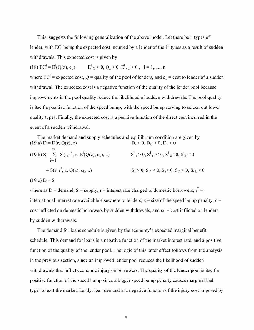
This, suggests the following generalization of the above model. Let there be n types of

lender, with ECi being the expected cost incurred by a lender of the ith types as a result of sudden

withdrawals. This expected cost is given by

(18) ECi = Ei(Q(z), cL) Ei Q < 0, Qz > 0, Ei cL > 0 , i = 1,....., n

where ECi = expected cost, Q = quality of the pool of lenders, and cL = cost to lender of a sudden

withdrawal. The expected cost is a negative function of the quality of the lender pool because

improvements in the pool quality reduce the likelihood of sudden withdrawals. The pool quality

is itself a positive function of the speed bump, with the speed bump serving to screen out lower

quality types. Finally, the expected cost is a positive function of the direct cost incurred in the

event of a sudden withdrawal.

The market demand and supply schedules and equilibrium condition are given by (19.a) D = D(r, Q(z), c) Dr < 0, DQ > 0, Dc < 0 n (19.b) S = ∑ Si(r, r*, z, Ei(Q(z), cL),...) Si r > 0, Si r* < 0, Si z< 0, Si

E < 0 i=1

= S(r, r*, z, Q(z), cL,...) Sr > 0, Sr* < 0, Sz< 0, SQ > 0, ScL < 0

(19.c) D = S

where as D = demand, S = supply, r = interest rate charged to domestic borrowers, r* =

international interest rate available elsewhere to lenders, z = size of the speed bump penalty, c =

cost inflicted on domestic borrowers by sudden withdrawals, and cL = cost inflicted on lenders

by sudden withdrawals.

The demand for loans schedule is given by the economy’s expected marginal benefit

schedule. This demand for loans is a negative function of the market interest rate, and a positive

function of the quality of the lender pool. The logic of this latter effect follows from the analysis

in the previous section, since an improved lender pool reduces the likelihood of sudden

withdrawals that inflict economic injury on borrowers. The quality of the lender pool is itself a

positive function of the speed bump since a bigger speed bump penalty causes marginal bad

types to exit the market. Lastly, loan demand is a negative function of the injury cost imposed by

10

sudden withdrawals. A lower injury cost (c) increases the return to borrowing, thereby increasing

demand for funds.

The supply of loans schedule is the sum of the loan supply schedules of different lender

types. Each individual type’s loan supply schedule is a positive function of the market interest

rate, a negative function of the interest rate available in international markets, a negative function

of the speed bump penalty cost, and a negative function of the expected cost inflicted by sudden

withdrawals by other lenders. The overall market supply of funds is a positive function of the

market interest rate, a negative function of the world interest rate, a negative function of the

speed bump penalty, a positive function of the quality of the pool of lenders, and a negative

function of the cost inflicted on lenders by sudden withdrawals.

The interesting feature of this loan supply schedule is that the speed bump has an ambiguous

effect on quantity supplied. Differentiating equation (19.b) with respect to z yields

dS/dz = Sz + SQQz >< 0

Thus, supply may either increase or decrease. A bigger speed bump penalty reduces quantity

supplied by directly reducing the expected return to lenders, but it also increases supply by

improving the quality of the lender pool which reduces withdrawal costs inflicted on good

lenders by sudden exits of bad lenders. This increases the expected return to good types, thereby

giving them an incentive to lend more. This latter effect shows how enhanced financial stability

can raise the supply of funds despite the fact that achieving it requires the imposition of speed

bump penalties which are a private cost.

These opposing effects (rate of return substitution versus financial stability) suggest that

imposing speed bumps may initially improve supply conditions by driving out the worst lender

types. However, as the level of the speed bump penalty is increased, this effect will reverse so

that further increases reduce supply. This in turn suggests that setting of the size of the speed

bump should be viewed as a policy choice problem, with the goal of policy makers being to

maximize the total expected returns provided by foreign borrowing.

Solving for the equilibrium and using the implicit function theorem enables solving for the

11

equilibrium interest rate schedule as a function of the exogenous variables. This equilibrium

interest rate schedule is given by

(20) r = r(z, c, cL, r* ) rz >< 0, rc > 0, rcL > 0, rr* > 0

The effect of a bigger speed bump on the equilibrium interest rate is ambiguous. Demand is

increased which unambiguously puts upward pressure on rates, but supply could fall which

would put downward pressure on rates. Henceforth, it is assumed that the demand side effect

dominates so that rz > 0.

The goal of the policy maker is to maximize the quantity of private borrowing to finance

private investment, which involves solving the following program (21) Max V = D( r(z, c, cL, r* ), Q(z), c) z

The first order condition is then given by

(22) dV/dz = Dr rz + DQQz = 0

The economic logic behind the above problem and its solution is illustrated in figure 4. The solid

lines represent the demand and supply schedules when there are no speed bumps, and the

equilibrium interest rate and quantity of short term foreign borrowing is determined by the

intersection of these schedules. The policy maker then adjusts the speed bump penalty which

shifts both the demand and supply schedules upward, and the penalty is increased at the margin

as long as it results in a larger marginal shift upward of the demand schedule than the supply

schedule. The final equilibrium is determined by the intersection of the new demand and supply

schedules given by the broken lines.

For an interior solution to exist for the above problem, increases in the size of the speed

bump (z) must initially shift the demand curve by more than they do the supply curve. However,

at some level of z, further marginal increases must shift the supply curve by more than they do

the demand curve. The logic for such a pattern is that at low levels of z, small increases cause the

most impatient investors to drop out but have little impact on good investors who plan to stay.

The supply schedule therefore shifts little, but the elimination of bad types who adversely affect

12

firms when they withdraw, has a large effect on demand. However, as z gets larger, it

increasingly impacts good types, thereby reversing the relative size of the impact on the demand

and supply of increases in z.

In sum, the above model illustrates how speed bumps can make an economy better off by

separating out bad lender types. Interestingly, speed bumps may actually increase foreign short

term borrowing despite the rise in interest rates. The reason is that the composition of lenders

shifts toward good types, which lowers the expected cost of sudden withdrawals, thereby raising

the benefit of borrowing. This result stands in contrast to the public finance account of speed

bumps. The reason is that a screening approach recognizes that speed bumps shift up both the

supply and demand schedules, whereas the public finance approach shifts up the supply schedule

only.

V Empirical evidence

The above investor screening model of capital flow speed bumps has two empirical

predictions. First, speed bumps should twist the composition of capital flows toward longer term

debt (the public finance effect). Second, speed bumps need not reduce the level of inflows, and

could even increase it (the screening effect). The case of Chile provides evidence that is

supportive of both of these propositions.

Chile introduced a 20% un-remunerated reserve requirement in June 1991. This reserve

requirement was increased to 30% on bank credit in August 1992. Subject to some further

administrative tightening, the system remained largely unchanged until December 1996, at which

time borrowing of less than $200,000 was exempted from the requirement. In March 1997 this

exemption was lowered to $100,00. In June 1998 the reserve requirement was set at 10%, and

finally in September 1998 it was set at zero.

Table 1 shows data on gross foreign capital inflows into Chile between 1990 and 1997.

Short term flows are defined as those having a contracted maturing of less than one year. The

immediately striking feature about this table is that there appears to have been a very sharp

reduction in the proportion of short term flows, and that reduction coincides exactly with the

13

introduction of un-remunerated reserve requirement on short term inflows.

Table 2 presents data on the maturity structure of Chilean external debt, and compares it

with that of the entire western hemisphere region as defined by the IMF. This definition includes

all countries except the U.S. and Canada. The western hemisphere grouping therefore serves as a

control for changes in general practices in financial markets. The table shows that over his period

the percentage of Chilean external debt that was short term tended to decline. The same is also

true for the western hemisphere group considered as a whole. However, the last column of table

2 shows that the decline was greater in Chile than in the western hemisphere region. This is

shown by the fact that the ratio of the percent of Chilean external debt that is short term to the

percent of western hemisphere external debt that is short term declined.

Finally, table 3 provides data on total private external debt in Chile and the western

hemisphere. Private external debt grew far more rapidly in Chile over the period 1990 - 97 than it

did in the western hemisphere as a whole. This superior relative performance of Chile is

consistent with the claim that speed bumps may actually increase total inflows by screening out

bad type investors and thereby increasing the return to good type investors who become willing

to invest more.

The data presented in tables 1 - 3 is of course just suggestive. Many factors have been at

work regarding both Chilean and western hemispheric capital inflows. However, it is at least re-

assuring that prima facie the data should be so supportive of the proposed screening mechanism

interpretation of speed bumps.

V Some further policy considerations

In the above model increases in the rate of return available in international markets (r*) cause

the supply schedule to shift up and reduce the availability of foreign funds. Such increases can

come from a strengthening of demand for funds in other national markets, or from structural

improvements in other markets that increase stability and returns there. In Chile, this is being

used as an argument to eliminate speed bumps, as evidenced by the following quote from the

Wall Street Journal:

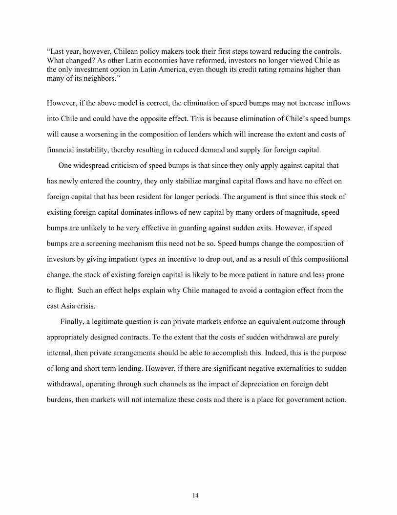
14

“Last year, however, Chilean policy makers took their first steps toward reducing the controls. What changed? As other Latin economies have reformed, investors no longer viewed Chile as the only investment option in Latin America, even though its credit rating remains higher than many of its neighbors.”

However, if the above model is correct, the elimination of speed bumps may not increase inflows

into Chile and could have the opposite effect. This is because elimination of Chile’s speed bumps

will cause a worsening in the composition of lenders which will increase the extent and costs of

financial instability, thereby resulting in reduced demand and supply for foreign capital.

One widespread criticism of speed bumps is that since they only apply against capital that

has newly entered the country, they only stabilize marginal capital flows and have no effect on

foreign capital that has been resident for longer periods. The argument is that since this stock of

existing foreign capital dominates inflows of new capital by many orders of magnitude, speed

bumps are unlikely to be very effective in guarding against sudden exits. However, if speed

bumps are a screening mechanism this need not be so. Speed bumps change the composition of

investors by giving impatient types an incentive to drop out, and as a result of this compositional

change, the stock of existing foreign capital is likely to be more patient in nature and less prone

to flight. Such an effect helps explain why Chile managed to avoid a contagion effect from the

east Asia crisis.

Finally, a legitimate question is can private markets enforce an equivalent outcome through

appropriately designed contracts. To the extent that the costs of sudden withdrawal are purely

internal, then private arrangements should be able to accomplish this. Indeed, this is the purpose

of long and short term lending. However, if there are significant negative externalities to sudden

withdrawal, operating through such channels as the impact of depreciation on foreign debt

burdens, then markets will not internalize these costs and there is a place for government action.

15

References Blecker, R.A., Taming Global Finance: A Better Architecture for Growth and Equity, Economic Policy Institute, Washington, DC, 1999. Council on Foreign Relations, “The Future of the International Financial Architecture: An Executive Summary of the Findings of a Council on Foreign Relations Task Force,” Foreign Affairs, 78 (November/December 1999), 169 - 184. Edwards, S., “How Effective are Capital Controls?” NBER Working Paper 7413, November 1999. De Gregorio, J., Edwards, S., and Valdes, O., “Controls on capital Inflows: Do They Work?” NBER Working Paper 7645, April 2000. Eichengreen, B., Toward a New International Financial Architecture: A Practical Post-Asia Agenda, Institute for International Economics, Washington, DC, 1999. Grabel, I., “Averting Crisis? Assessing Measures to Mange Financial Integration in Emerging Economies,” Cambridge Journal of Economics, forthcoming 2002/03. Palley, T.I., “International Finance and Global Deflation: There is an Alternative,” in Michie, J., and Grieve-Smith, J. (eds.), Global Instability: The Political Economy of World Economic Governance, New York: Routledge, 1999. “Investors to Watch Chile’s Presidential Election As Candidates Pledge to Kill Controls on Capital,” Wall Street Journal, Monday 10 January, 2000.

16

Interest rate (%)

r*/[1-k]

r*

D(.)

D1D0 Quantity ($)

Figure 1 The public finance approach to speed bumps showing how they raiseinterest rates and reduce the amount of borrowing.

17

Interest rate (%)

r*

D1(.)

D0(.)

D1 Quantity ($)

Figure 2 No speed bump equilibrium in a world where borrowers cannot distinguishbetween good (patient) and bad (impatient) lenders.

18

Interest rate (%)

rA

r*

D1(.)D2(.)

D0(.)

Quantity ($)D1 D2

Figure 3 Speed bump equilibrium in which bad (impatient) lenders are screened out of the market.

19

Interest rate (%)

r2

r1

S2(.)

S1(.)

D2(.)D1(.)

Quantity ($)D1 D2

Figure 4 Speed bump equilibrium in a model with many types of lender and anupward sloping capital supply schedule.

20

Table 1 Gross foreign capital inflows ($ millions)into Chile, 1990 - 97.

Year Short term flows % of total Long term flows % of total Total flows

1990 1,683,149 90.3 181,419 9.7 1,864,568

1991 521,198 72.7 196,115 27.3 717,313

1992 225,197 28.9 554,072 71.1 779,269

1993 159,462 23.6 515,147 76.8 674,609

1994 161,575 16.5 819,699 83.5 981,274

1995 69,675 6.2 1,051,829 93.8 1,121,504

1996 67,254 3.2 2,042,456 96.8 2,109,710

1997 81,131 2.8 2,887,013 97.2 2,887,013

Source: Edwards, 1999.

21

Table 2 Comparison of Chilean external debt and debt structure versus Western hemisphere region. <------- Chile ($ millions)---------> <-- Western Hemisphere ($ billions)--> Ratio Total external Short % short Total external Short % short % Short Chile:

Debt Term Term Debt Term Term % Short W.Hemis.

1990 17,425 3,382 19.4 440.8 75.0 17.0 1.14

1991 16,364 2,199 13.4 463.0 86.0 18.6 0.72

1992 18,242 3,475 19.0 492.1 86.8 17.6 1.08

1993 19,186 3,487 18.2 537.8 91.3 17.0 1.07

1994 21,478 3,865 18.0 580.7 91.1 15.7 1.15

1995 21,736 3,431 15.8 641.4 106.6 16.6 0.95

1996 22,979 2,635 11.5 659.4 99.0 15.0 0.77

1997 26,701 1,287 4.8 682.2 85.3 12.5 0.38

Source: De Gregorio et al., 2000: IMF World Economic Outlook, May 1998, and author’s calculations.

22

Table 3 Total private external debt and annual growth <--------Chile------------> <--Western Hemisphere–> Private debt Annual Private debt Annual ($ millions) % change ($ billions) % change

1990 5,633 – 296.4 --

1991 5,810 3.1 304.6 2.8

1992 8,619 48.3 331.4 8.8

1993 10,166 17.9 377.2 13.8

1994 12,343 21.4 411.6 9.1

1995 14,235 15.3 447.2 8.6

1996 17,816 25.2 476.4 6.5

1997 21,613 21.3 515.4 8.2

Source: De Gregorio at al., 2000, IMF World Economic Outlook, May 1998, and author’s calculations.