CHARACTERIZATION AND MODELING OF TWO-PHASE HEAT
202
ABSTRACT Title of Document: CHARACTERIZATION AND MODELING OF TWO-PHASE HEAT TRANSFER IN CHIP- SCALE NON-UNIFORMLY HEATED MICROGAP CHANNELS Ihab A. Ali, Doctor of Philosophy, 2010 Directed By: Professor Avram Bar-Cohen Department of Mechanical Engineering A chip-scale, non-uniformly heated microgap channel, 100 micron to 500 micron in height with dielectric fluid HFE-7100 providing direct single- and two-phase liquid cooling for a thermal test chip with localized heat flux reaching 100 W/cm 2 , is experimentally characterized and numerically modeled. Single-phase heat transfer and hydraulic characterization is performed to establish the single-phase baseline performance of the microgap channel and to validate the mesh-intensive CFD numerical model developed for the test channel. Convective heat transfer coefficients for HFE-7100 flowing in a 100-micron microgap channel reached 9 kW/m 2 K at 6.5 m/s fluid velocity. Despite the highly non-uniform boundary conditions imposed on the microgap channel, CFD model simulation gave excellent agreement with the experimental data (to within 5%), while the discrepancy with the predictions of the classical, “ideal” channel correlations in the literature reached 20%.
Transcript of CHARACTERIZATION AND MODELING OF TWO-PHASE HEAT
ABSTRACT
Title of Document: CHARACTERIZATION AND MODELING OF
TWO-PHASE HEAT TRANSFER IN CHIP-
SCALE NON-UNIFORMLY HEATED
MICROGAP CHANNELS
Ihab A. Ali, Doctor of Philosophy, 2010
Directed By: Professor Avram Bar-Cohen
Department of Mechanical Engineering
A chip-scale, non-uniformly heated microgap channel, 100 micron to 500
micron in height with dielectric fluid HFE-7100 providing direct single- and two-phase
liquid cooling for a thermal test chip with localized heat flux reaching 100 W/cm2, is
experimentally characterized and numerically modeled. Single-phase heat transfer and
hydraulic characterization is performed to establish the single-phase baseline
performance of the microgap channel and to validate the mesh-intensive CFD
numerical model developed for the test channel. Convective heat transfer coefficients
for HFE-7100 flowing in a 100-micron microgap channel reached 9 kW/m2K at 6.5
m/s fluid velocity. Despite the highly non-uniform boundary conditions imposed on
the microgap channel, CFD model simulation gave excellent agreement with the
experimental data (to within 5%), while the discrepancy with the predictions of the
classical, “ideal” channel correlations in the literature reached 20%.
A detailed investigation of two-phase heat transfer in non-ideal micro gap
channels, with developing flow and significant non-uniformities in heat generation,
was performed.
Significant temperature non-uniformities were observed with non-uniform heating,
where the wall temperature gradient exceeded 30°C with a heat flux gradient of 3-30
W/cm2, for the quadrant-die heating pattern compared to a 20°C gradient and 7-14
W/cm2 heat flux gradient for the uniform heating pattern, at 25W heat and 1500
kg/m2s mass flux.
Using an inverse computation technique for determining the heat flow into the wetted
microgap channel, average wall heat transfer coefficients were found to vary in a
complex fashion with channel height, flow rate, heat flux, and heating pattern and to
typically display an inverse parabolic segment of a previously observed M-shaped
variation with quality, for two-phase thermal transport. Examination of heat transfer
coefficients sorted by flow regimes yielded an overall agreement of 31% between
predictions of the Chen correlation and the 24 data points classified as being in
Annular flow, using a recently proposed Intermittent/Annular transition criterion. A
semi-numerical first-order technique, using the Chen correlation, was found to yield
acceptable prediction accuracy (17%) for the wall temperature distribution and hot
spots in non-uniformly heated “real world” microgap channels cooled by two-phase
flow.
Heat transfer coefficients in the 100-micron channel were found to reach an
Annular flow peak of ~8 kW/m2K at G=1500 kg/m
2s and vapor quality of x=10%. In a
500-micron channel, the Annular heat transfer coefficient was found to reach 9
kW/m2K at 270 kg/m
2s mass flux and 14% vapor quality level. The peak two-phase
HFE-7100 heat transfer coefficient values were nearly 2.5-4 times higher (at similar
mass fluxes) than the single-phase HFE-7100 values and sometimes exceeded the
cooling capability associated with water under forced convection. An alternative
classification of heat transfer coefficients, based on the variable slope of the observed
heat transfer coefficient curve), was found to yield good agreement with the Chen
correlation predictions in the pseudo-annular flow regime (22%) but to fall to 38%
when compared to the Shah correlation for data in the pseudo-intermittent flow regime.
CHARACTERIZATION AND MODELING OF TWO-PHASE HEAT TRANSFER
IN CHIP-SCALE NON-UNIFORMLY HEATED MICROGAP CHANNELS
by
Ihab A. Ali
Dissertation submitted to the Faculty of the Graduate School of the
University of Maryland, College Park, in partial fulfillment
Of the requirements for the degree of
Doctor of Philosophy
2010
Advisory Committee:
Professor Avram Bar-Cohen, Chair
Professor Marino DiMarzo
Professor Patrick McCluskey
Professor Peter Sandborn
Professor Bao Yang
Professor Gary Pertmer

© Copyright by
Ihab A. Ali
2010

ii
Dedication
To my sister Rola
Your Soul will inspire us and be in our hearts forever.

iii
Acknowledgements
Thank you my advisor Professor Avram Bar-Cohen for your advice, wisdom and
support throughout the years of this work. I would like to thank my committee
members, Professor Marino DiMarzo, Professor Patrick McCluskey, Professor Peter
Sandborn, Professor Bao Yang and Professor Gary Pertmer, for their great comments,
support and advice.
Many thanks to my friends Emil Rahim, Vinh Nguyen, Henry Lam, William Maltz,
Ceferino Sanchez, Dr. Attila Aranyosi, Juan Cruz, Dr. Himanshu Pokharna, Dr. Rajiv
Mongia, Dr. Jay Nigen and Bernie Rihn.
I have great gratitude to the Advanced Cooling Technologies’ (ACT) Dr. Jon Zuo, Mr.
Richard Bonner, Mr. John Hartenstine and especially my dear friend Mr. Scott Garner
for their great efforts and support with the design of the apparatus used in this
research.
Special thanks to Mr. Phil Tuma of 3M for his technical support and donation of the
HFE-7100 fluid used in this work.
Thanks to my late sister Rola, your soul inspired and enriched me to stay in course
until the end. Thanks to my mother Sabiha, my father Abdulkarim, my sisters Heba
and Reem, my brother Hossam and my nephews Hasan and Hany. I love you.
Thank you my wife Alia and my son Sammy for your support and love. I am sorry for
not been able to spend enough time with you the past few years. You are my life.
iv
Table of Contents
Dedication………………………………………………………………………...…….v
Acknowledgements ………………………………………………………………......vi
Table of Contents…………………………………………...…………………...........vii
List of Tables………………………………………………………………..................xi
List of Figures…………………….…………………………………………..............xiv
1. Trends and Cooling Requirements in the Electronic Industry………………...…….1
2. Liquid Cooling of Electronic Modules – Literature Review……………………….10
2.1 Introduction………………...………………………………………..........10
2.2 Microchannel Coolers………………………………..…………......…….11
2.3 Pool Boiling................................................................................................14
2.4 Liquid Immersion Cooling…………………………………………….....16
2.5 Liquid Immersion Modules........................................................................18
2.6 Flow Boiling...............................................................................................20
3. Theoretical Background............................................................................................23
3.1 Single Phase Thermofluid Characteristics in Miniature Channels.............23
3.1.1 Pressure drop correlations…………………………………...….23
3.2.2 Heat transfer correlations……………………………………….25
3.3.3 Effect of heating non-uniformity……………………………….27
3.2 Two-Phase Thermofluid Characteristics in Miniature Channels…..……..28
3.2.1 Introduction………………………………………………...…...28
v
3.2.2 Two-phase flow regime modeling………………………………31
3.2.3 Characteristics of two-phase heat transfer in micro channels…..34
3.2.4 Heat transfer correlations…………………………..………...…35
3.2.5 Unresolved issues in two-phase behavior in microgaps………...41
4. Experimental Apparatus ………………………………………………………….43
4.1 Overall Description……………………………………………………….43
4.2 Calibration of Flow Meter ……………………………………………….45
4.3 Chip Thermal Test Vehicle…………………………...…………………..46
4.4 The Microgap Test Channel… …………………………………………..52
4.5 Chip TTV - Sensor Calibration Procedure………………………………..53
4.6 Fluid Selection and HFE-7100 Novec Properties…………………………54
5. CFD Model and Simulation…………………………………...……………………59
5.1 Introduction……………………………………………………………….59
5.2 Equations Solved and Methodology………………………………………59
5.3 Model Description and Conjugate Heat Transfer………….……………...61
6. Single-Phase Data and Discussion……………………..…………………………..67
6.1 Basic Relations…………………………..………………………………..67
6.2 Error Analysis……………………………………………………………..68
6.3 Single Phase Results………………………………………………………70
6.3.1 Comparison of experimental, CFD and theoretical correlation....70
6.3.2 Raw temperature data and comparison to CFD………………....76
6.3.3 Conjugate effects and conduction spreading in advanced
vi
microprocessors……………………………………………………….82
6.3.4 Temperature distribution – Uniform heating….………………...89
6.3.5 Temperature Distribution - Half-die and quadrant-die heating…93
6.3.6 Inversely determined heat transfer coefficients………………....95
6.4 Overall Single-Phase Hydraulic and Thermal Performance…….………...98
6.5 Conclusions……………………………………………………………...102
7. Two-Phase Heat Transfer Experimental Data and Discussion……………………106
7.1 Introduction and Basic Relations………………..…………………….…106
7.2 Taitel-Dukler Flow Regime Map………………………………………..111
7.3 Heat Transfer Characteristics…………………………….……………...125
7.4 Heat transfer Characteristics with Non-Uniform Heating……………….131
8. Heat Transfer Correlations……………………………………………………..…136
8.1 Introduction……………………………………………………………...136
8.2 Heat Transfer Correlation Based on Two-Phase Reynolds Number……137
8.3 Flow Regime Sorting Based on TD Transition Line……………………138
8.4 Flow Regime Sorting Based on Characteristic Curve…………………...142
8.5 Inverse Calculations of Spatial Heat Transfer Coefficient………………147
8.6 Inverse Calculations of Spatial Chen-Based Heat Transfer Coefficient...152
8.7 Prediction of Wall Temperature Distribution and Hot spots of Non-uniform
Heating………………………………………………………………..……..155
8.8 Conclusions…………………………………………………………..….158
9. Conclusion and Future Work………………….………………………………….164

vii
9.1 Conclusion……………………………………………………………….164
9.2 Future Work…..…………………………………………………………171
10. Bibliography………………………………….……………………………….....174
viii
List of Tables
Table 1: HFE-7100 Environmental Properties [52]. ...................................................55
Table 2: HFE-7100 Toxicity Properties [52]. .............................................................56
Table 3: Characteristics of 3M’s Fluorinert and Novec Fluids [52]. ...........................57
Table 4: HFE-7100 Thermo-Physical Properties Compared to Other Coolants...........58
Table 5: Sensor Temperatures for the Uniformly Heated 100-micron Microgap
Channel with the Flow of HFE-7100, Tin=23°C, q!=7W/cm2. ..........................77
Table 6: Sensor Temperatures for the Half-Die Heated 100-micron Microgap Channel
with the Flow of HFE-7100, Tin=23°C, q!=7W/cm2. ........................................78
Table 7: Sensor Temperatures for the Quadrant-Die Heated 100-micron Microgap
Channel with the Flow of HFE-7100, Tin=23°C, q!=7W/cm2. ..........................78
Table 8: Sensor Temperatures vs. Flow Rates and Junction vs. Surface (Wall)
Temperatures for 100-micron Channel and Uniform Heating with the flow of
HFE-7100, Tin=23°C, q!=7W/cm2....................................................................81
Table 9: Sensor Temperatures vs. Flow Rates and Junction vs. Surface (Wall)
Temperatures for 100-micron Channel and Half-Die Heating with the flow of
HFE-7100, Tin=23°C, q!=7W/cm2....................................................................81
Table 10: Sensor Temperatures vs. Flow Rates and Junction vs. Surface (Wall)
Temperatures for 100-micron Channel and Quadrant-Die Heating with the flow
of HFE-7100, Tin=23°C, q!=7W/cm2. ..............................................................82
ix
Table 11: Average error (
!
"AVE ) of Heat transfer Coefficient Predictions Sorted by
Annular and Intermittent Flow Regimes per Classical T&D Line and
!
We1/ 2
Bo1/ 4
= 6.2
Based Line-Uniformly-Heated Channel. ..........................................................139
Table 12: Parameters of Two-Phase Heat Transfer Chen Correlation on 100-micron
Channel, Showing Error Reduction by Setting Convective Enhancement Term
F=1..................................................................................................................141
Table 13: Average Error (
!
"AVE ) of Heat Transfer Coefficient Predictions Using Chen
and Shah Correlations for Uniformly Heated Channels. ...................................143
Table 14: Average Error (
!
"AVE ) of Heat Transfer Coefficient Predictions Sorted by
Pseudo Annular and Pseudo Intermittent Flow regimes Graphically per (h vs. x)
Characteristic Curve, for Uniformly Heated Channels......................................144
Table 15: Average Error (
!
"AVE ) of Heat Transfer Coefficient Predictions Using Chen
and Shah Correlations for Half-Die Heated Channels.......................................144
Table 16: Average Error (
!
"AVE ) of Heat Transfer Coefficient Predictions Sorted by
Pseudo Annular and Pseudo Intermittent Flow regimes Graphically per (h vs. x)
Characteristic Curve, for Half-Die Heated Channels. .......................................145
Table 17: Average Error (
!
"AVE ) of Heat Transfer Coefficient Predictions Using Chen
and Shah Correlations for Quadrant Heated Channels. .....................................145
Table 18: Average Error (
!
"AVE ) of Heat Transfer Coefficient Predictions Sorted by
Pseudo Annular and Pseudo Intermittent Flow regimes Graphically per (h vs. x)
Characteristic Curve, for Quadrant Heated Channels........................................146
x
Table 19: Experimental (Two-Phase Test) and Iteratively Adjusted CFD Wall
Temperatures for Three Heating Patterns. 100 micron Channel, 25W, G= 1500
kg/m2s.............................................................................................................149
Table 20: Temperature Errors of Conduction-Only Model with Prescribed Chen-Based
Average h on Wall, 100-micron Channel Flowing HFE-7100, P=25W, G= 1500
kg/m2s.............................................................................................................158
xi
List of Figures
Figure 1: iNEMI’s Server Chip power and Heat Flux Trends [1]. ................................1
Figure 2: ITRS Power Trend for High Performance and Cost Performance Electronic
Chips [2]..............................................................................................................2
Figure 3: Trends in Chip Package Thermal Resistance [3]. ..........................................3
Figure 4: Power Non-Uniformity of Intel’s Itanium Processor [4]................................4
Figure 5: Power Map (Non-Uniformity) Impact on Thermal and Cooling Performance
[4]........................................................................................................................5
Figure 6: Thermal Packaging Roadmap 2001-2016 [5] ................................................6
Figure 7: Hot spot cooling by microchannel liquid cooled plate mounted on chip
substrate via TIM layer [6].................................................................................10
Figure 8: High Power IGBT Module [7]. ...................................................................11
Figure 9: Integrated Liquid (R134a) Cooled Plate for IGBT Module [7]. ...................12
Figure 10: Server Rack-Level Cooling for Stacked IGBT Modules [7] ......................12
Figure 11: Two-phase Flow regimes in horizontal channel [20]. ................................30
Figure 12: Taitel-Dukler Flow Regime Map Showing, Stratified, Bubble, Intermittent
and Annular Flow Regimes- 100-micron Channel Dh=200 micron, HFE-7100
Fluid. .................................................................................................................31
Figure 13: Heat transfer coefficient data from Yang and Fujita [37] and Cortina-Diaz
and Schmidt [38] showing the characteristic M-shape behavior [20]. .................33
Figure 14: Two-Phase Microgap Channel Test Apparatus..........................................43
xii
Figure 15: Design Schematics of the Two-Phase Microgap Channel Apparatus .........44
Figure 16: External Water-Cooled Condenser for the two-Phase Microgap Channel
Apparatus. .........................................................................................................45
Figure 17: Pressure Relief Reservoir for the two-Phase Microgap Channel Apparatus.
..........................................................................................................................46
Figure 18: Kobold Flow Meter Calibration Curves for Water and HFE-7100.............47
Figure 19: Intel’s Merom Processor Thermal Test Vehicle (TTV) [51]. .....................48
Figure 20: Intel’s TTV Schematic Three Different Power (Heating) Zones with
Locations of Temperature Sensors. ....................................................................48
Figure 21: Intel’s TTV Serpentine-Type Heating Zones and Locations of Temperature
Sensors [51].......................................................................................................49
Figure 22: Assembled Intel TTV Showing Locations of the Three Heater Zones. ......50
Figure 23: Intel’s TTV Board. ...................................................................................51
Figure 24: TTV Cooper Channel ...............................................................................52
Figure 25: Hermetically Sealed Microgap Channel. ...................................................52
Figure 26: TTV Characteristic Temperature Sensor Calibration.................................53
Figure 27: HFE-7100 Thermal and Fluid Properties [52]. ..........................................58
Figure 28: The CFD Computational Grid...................................................................61
Figure 29: Fluid Channel Grid. ..................................................................................62
Figure 30: Full Conjugate Domain Grid.....................................................................63
Figure 31: CFD Solution Convergence for Key Temperature Sensors........................63
Figure 32: 3-D View of the Microgap Fluid Channel CFD Model..............................64
xiii
Figure 33: XY and YZ Views of the Microgap Fluid Channel CFD Model. ...............65
Figure 34: Model of the Junction Plane Showing the Emulated Serpentine-Type
Heating Zones....................................................................................................66
Figure 35: Effect of Fluid Velocity on Single-Phase Pressure Drop in a 100-micron
Microgap Channel Flowing HFE-7100 (Dh = 200 micron). ...............................72
Figure 36: Effect of Fluid Velocity on Single-Phase Heat Transfer Coefficient in a
100-micron Microgap Channel Flowing HFE-7100 (Dh = 200 micron). P=10W,
Tin=23C. ...........................................................................................................73
Figure 37: Single-Phase Pressure Drop vs. Velocity for HFE-7100 in a 100-micron
Microgap Channel (Dh=200 micron). ................................................................75
Figure 38: Single-Phase Heat Transfer Coefficient vs. Velocity for HFE-7100 in a 100-
micron Microgap Channel (Dh=200 micron). P=10W, Tin=23C........................76
Figure 39: Die Average Sensor Excess Temperature Test Data and CFD Simulation vs.
Velocity, HFE-7100 flowing in a 100-micron Microgap Channel and Uniform
Heating q!=7W/cm2. .........................................................................................79
Figure 40: Conduction Spreading Conjugate Effect on Wall Spatial Heat Flux and
Heat Transfer Coefficient for Uniformly Heated 100-micron Channel with the
Flow of HFE-7100, Tin=23°C, q!=7W/cm2.......................................................84
Figure 41: Conduction Spreading Conjugate Effect on Wall Spatial Heat Flux and
Heat Transfer Coefficient for Half-Die Heated 100-micron Channel with the Flow
of HFE-7100, Tin=23°C, q!=7W/cm2. ..............................................................85
xiv
Figure 42: Conduction Spreading Conjugate Effect on Wall Spatial Heat Flux and
Heat Transfer Coefficient for Quadrant-Die Heated 100-micron Channel with the
Flow of HFE-7100, Tin=23°C, q!=7W/cm2.......................................................86
Figure 43: Single-Phase Conjugate Heat Transfer Conversion Rate vs. Fluid Inlet
Velocity for the 100-micron Microgap Channel. P=10W, Tin=23C....................89
Figure 44: Chip Surface (Wall) Temperature Distribution of Uniformly Heated 100-
micron Microgap Channel - (a) 0.7m/s (left), (b) 6.5m/s (right), Tin =23C.........92
Figure 45: Mid-Height Fluid Velocity Vectors Distribution for a 100-micron
Uniformly Heated Microgap Channel - (a) 0.7m/s (left), (b) 6.5m/s (right). .......92
Figure 46: Mid-Height Pressure Distribution for a 100-micron Uniformly Heated
Microgap Channel - (a) 0.7m/s (left), (b) 6.5m/s (right). ....................................93
Figure 47: Chip Surface (Wall) Temperature Distribution of Half-Die Heated 100-
micron Microgap Channel - (a) 0.7m/s (left), (b) 6.5m/s (right), Tin=23C..........94
Figure 48: Chip Surface (Wall) Temperature Distribution of Quadrant-Die Heated
100-micron Microgap Channel - (a) 0.7m/s (left), (b) 6.5m/s (right), Tin=23C...95
Figure 49: Spatial Variation of Heat Transfer Coefficient for Uniformly Heated 100-
micron Microgap Channel - (a) 0.7m/s (left), (b) 6.5m/s (right), Tin=23C..........96
Figure 50: Spatial Variation of Heat Transfer Coefficient for Half-Die Heated 100-
micron Microgap Channel - (a) 0.7m/s (left), (b) 6.5m/s (right), Tin=23C..........97
Figure 51: Spatial Variation of Heat Transfer Coefficient for Quadrant-Die Heated
100-micron Microgap Channel - (a) 0.7m/s (left), (b) 6.5m/s (right), Tin=23C...97
xv
Figure 52: Pressure Drop vs. Re for a Microgap Channel with Various Channel
Heights, flowing HFE-7100, Tin=23°C, q!=7W/cm2.......................................100
Figure 53: Heat Transfer Coefficient vs. Re for a Microgap Channel with Various
Channel Heights, flowing HFE-7100, Tin=23°C, q!=7W/cm2. ........................101
Figure 54: Pressure Drop vs. Re for a Microgap Channel with Various Channel
Heights, flowing Water, Tin=23°C, q!=7W/cm2..............................................102
Figure 55: Heat Transfer Coefficient vs. Re for a Microgap Channel with Various
Channel Heights, flowing Water, Tin=23°C, q!=7W/cm2. ...............................102
Figure 56: Two-phase h vs. q! and x for Uniform Heated 100-micron Channel Flowing
HFE-7100........................................................................................................110
Figure 57: Two-phase h vs. q! and x for Uniform Heated 200-micron Channel Flowing
HFE-7100........................................................................................................111
Figure 58: Two-phase h vs. q! and x for Uniform Heated 500-micron Channel Flowing
HFE-7100........................................................................................................111
Figure 59: Taitel-Dukler Map with Flow Regimes and h’s for Uniform Heating and
100-micron Channel. G=350, 500, 650, 800, 1000 and 1500 kg/m2s................113
Figure 60: Taitel-Dukler Map with Flow Regimes and h’s for Uniform heating and
200-micron Channel. G=150, 350, 500, 650, 800, 1000 and 1500 kg/m2s........114
Figure 61: Taitel-Dukler Map with Flow Regimes and h’s for Uniform Heating and
500-micron Channel. G=80, 150, 270 and 350 kg/m2s.....................................115
Figure 62: Tabatabai & Faghri’s Modification to the Taitel-Dukler Map Showing the
Proposed Transition Line to Annular Flow [20]. ..............................................117
xvi
Figure 63: Taitel-Dukler Map with Flow Regimes and h’s for Half-Die Heating and
100-micron Channel. G=350, 500, 650, 800, 1000 and 1500 kg/m2s................120
Figure 64: Taitel-Dukler Map with Flow Regimes and h’s for Half-Die Heating and
200-micron Channel. G=150, 350, 500, 650, 800 and 1500 kg/m2s..................121
Figure 65: Taitel-Dukler Map with Flow Regimes and h’s for Half-Die Heating and
500-micron Channel. G=80, 150, 270 and 350 kg/m2s.....................................122
Figure 66: Taitel-Dukler Map with Flow Regimes and h’s for Quadrant-Die Heating
and 100-micron Channel. G=350, 500, 650, 800, 1000 and 1500 kg/m2s. ........123
Figure 67: Taitel-Dukler Map with Flow Regimes and h’s for Quadrant-Die Heating
and 200-micron Channel. G=150, 350, 500, 650, 800, 1000 and 1500 kg/m2s. 124
Figure 68: Taitel-Dukler Map with Flow Regimes and h’s for Quadrant-Die Heating
and 500-micron Channel. G=80, 150, 270 and 350 kg/m2s. .............................125
Figure 69: Two-Phase h vs. Exit Quality x of the Yang&Fujita [37] and Diaz et al [38]
Data [20]. ........................................................................................................127
Figure 70: Two-Phase h vs. Exit Quality x of the Uniformly Heated 100-micron
Microgap Channel. ..........................................................................................128
Figure 71: Two-Phase h vs. Exit Quality x of the Uniformly Heated 200-micron
Microgap Channel. ..........................................................................................129
Figure 72: Two-Phase h vs. Exit Quality x of the Uniformly Heated 500-micron
Microgap Channel. ..........................................................................................130
Figure 73: Two-Phase h vs. q and x for Half-Die Heating and 100-micron Channel.131
Figure 74: Two-Phase h vs. q and x for Half-Die Heating and 200-micron Channel.132
xvii
Figure 75: Two-Phase h vs. q and x for Half-Die Heating and 500-micron Channel.132
Figure 76: Two-Phase h vs. q and x for Quadrant-Die Heating and 100-micron
Channel. ..........................................................................................................133
Figure 77: Two-Phase h vs. q and x for Quadrant-Die Heating and 200-micron
Channel. ..........................................................................................................133
Figure 78: Two-Phase h vs. q and x for Quadrant-Die Heating and 500-micron
Channel. ..........................................................................................................134
Figure 79: Two-Phase Heat Transfer Coefficient versus Retp for the Uniformly
Heated 100-micron Microgap Channel.............................................................138
Figure 80: Characteristic Heat Transfer Coefficient Curve with Illustrated Ranges of
Pseudo Annular and Pseudo Intermittent Flow Regimes, Uniformly-Heated 100-
micron Channel, G =1500 kg/m2s....................................................................143
Figure 81: Inversely Calculated Spatial Heat Transfer Coefficient for 100-micron
Channel and Uniform Heating. 25W, G= 1500 kg/m2s. ...................................150
Figure 82: Inversely Calculated Spatial Heat Transfer Coefficient for 100-micron
Channel and Half-Die Non-Uniform Heating. 25W, G= 1500 kg/m2s..............151
Figure 83: Inversely Calculated Spatial Heat Transfer Coefficient for 100-micron
Channel and Quadrant-Die Non-Uniform Heating. 25W, G= 1500 kg/m2s. .....152
Figure 84: Inversely Calculated Chen-based Spatial Heat Transfer Coefficient for 100-
micron Channel and Uniform Heating. 25W, G= 1500 kg/m2s. .......................154
Figure 85: Inversely Calculated Chen-based Spatial Heat Transfer Coefficient for 100-
micron Channel and Half-Die Non-Uniform Heating. 25W, G= 1500 kg/m2s..155

xviii
Figure 86: CFD Temperature Distribution vs. Conduction-Only Based Modeling with
Wall-Prescribed Average Chen-Based h. 25W, G= 1500 kg/m2s. ....................157
1
Chapter 1:
Trends and Cooling Requirements in the Electronic Industry
In recent decades the industry-wide trend in electronics has been toward greater
compactness, functionality and feature count and thus power dissipation for nearly all
the categories of electronic equipment. The International Electronics Manufacturing
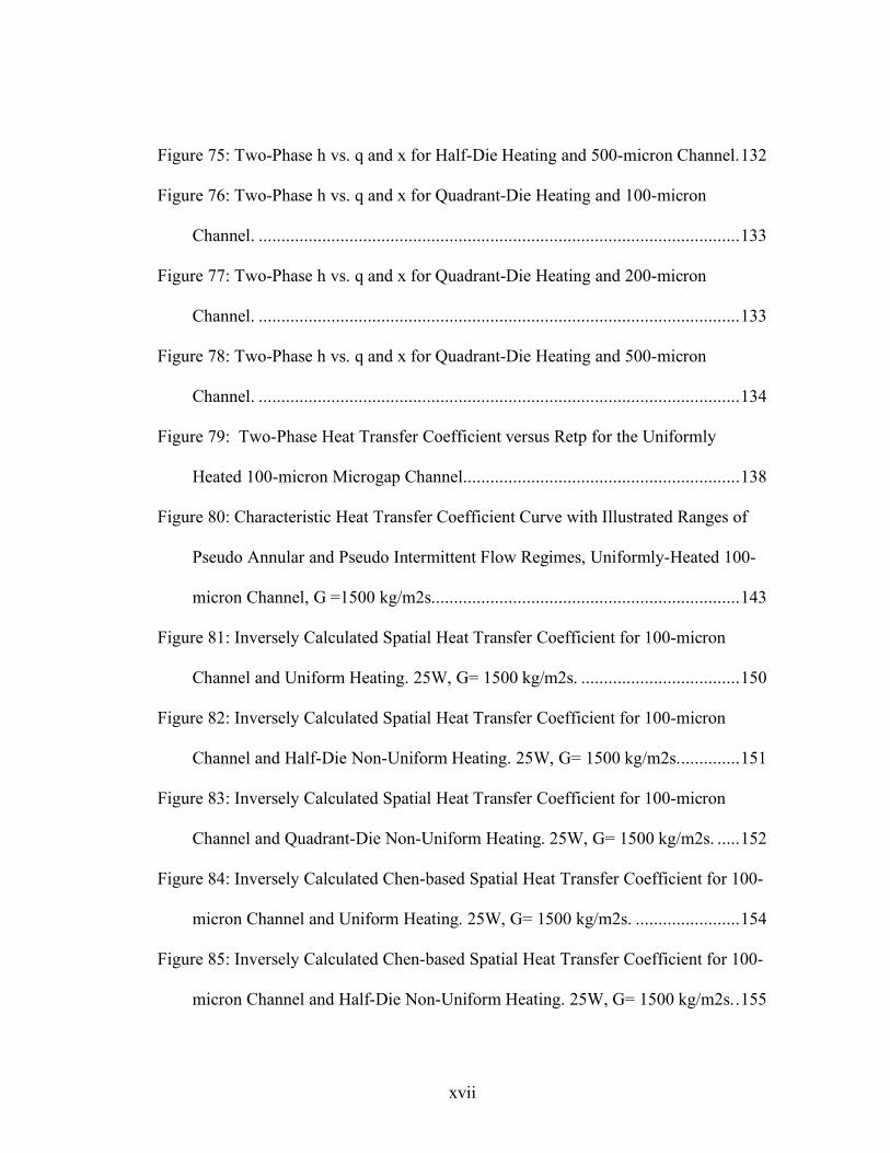
Initiative (iNEMI) projects the chip power and chip heat flux trends for various
electronic enclosure form factors, from servers to notebook platforms. Figure 1 shows
the iNEMI’s view of chip power chip flux trends for server platforms [1]. It is quite
clear from the figure that the market shall, if it has not already, experience
unprecedented growth in chip power and heat flux that by 2012 could reach 300W and
150 W/cm2 in heat dissipation and heat flux, respectively.
Figure 1: iNEMI’s Server Chip power and Heat Flux Trends [1].
2
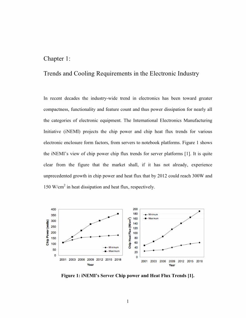
Although the increased awareness of power consumption and efforts to develop more
energy efficient devices will cause this rate to slow, as per the International
Technology Roadmap for Semiconductor (ITRS) shown in Figure 2, for the cost-
performance system category, this slow down might not become apparent until the
year 2015 [2]. On the other hand, changes in chip layout and packaging technologies,
throughout recent years, have led to the wide adoption of flip chip technology and the
appearance of highly non-uniform chip power dissipation. Both of these trends have
had a strong impact on thermal management needs and thermal design constraints on
advanced chip packages.
Figure 2: ITRS Power Trend for High Performance and Cost Performance
Electronic Chips [2].
3
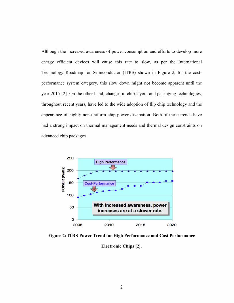
As shown in Figure 3, in the past decade thermal management of flip chip dies with
non-uniform power dissipation has focused on the need to significantly lower the
maximum chip-to-heat sink thermal resistance. Continuously improving heat sink
performance has
made the chip-to-heat sink resistance dominant and the “controlling” or critical
element of the total system thermal resistance [3]. Efforts must thus be directed at
minimizing the chip-to-sink thermal resistance. Note that the arrow and circle in
Figure 3 refer the thermal resistance curve to the year 2005, when the reference was
published.
Figure 3: Trends in Chip Package Thermal Resistance [3].
The issue of chip power non-uniformity or non-uniform die heat flux is a frequent
subject of the recent electronics cooling literature [4]. Figure 4 displays the heat flux
4
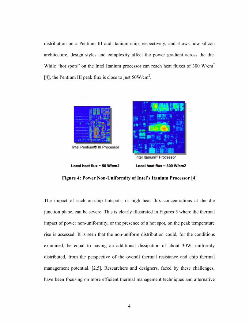
distribution on a Pentium III and Itanium chip, respectively, and shows how silicon
architecture, design styles and complexity affect the power gradient across the die.
While “hot spots” on the Intel Itanium processor can reach heat fluxes of 300 W/cm2
[4], the Pentium III peak flux is close to just 50W/cm2.
Figure 4: Power Non-Uniformity of Intel’s Itanium Processor [4]
The impact of such on-chip hotspots, or high heat flux concentrations at the die
junction plane, can be severe. This is clearly illustrated in Figures 5 where the thermal
impact of power non-uniformity, or the presence of a hot spot, on the peak temperature
rise is assessed. It is seen that the non-uniform distribution could, for the conditions
examined, be equal to having an additional dissipation of about 30W, uniformly
distributed, from the perspective of the overall thermal resistance and chip thermal
management potential. [2,5]. Researchers and designers, faced by these challenges,
have been focusing on more efficient thermal management techniques and alternative
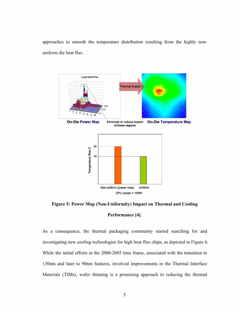
5
approaches to smooth the temperature distribution resulting from the highly non-
uniform die heat flux.
Figure 5: Power Map (Non-Uniformity) Impact on Thermal and Cooling
Performance [4].
As a consequence, the thermal packaging community started searching for and
investigating new cooling technologies for high heat flux chips, as depicted in Figure 6.
While the initial efforts in the 2000-2005 time frame, associated with the transition to
130nm and later to 90nm features, involved improvements in the Thermal Interface
Materials (TIMs), wafer thinning is a promising approach to reducing the thermal
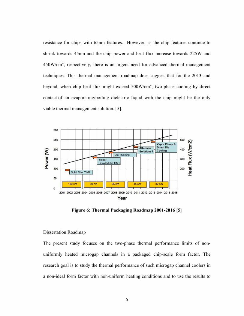
6
resistance for chips with 65nm features. However, as the chip features continue to
shrink towards 45nm and the chip power and heat flux increase towards 225W and
450W/cm2, respectively, there is an urgent need for advanced thermal management
techniques. This thermal management roadmap does suggest that for the 2013 and
beyond, when chip heat flux might exceed 500W/cm2, two-phase cooling by direct
contact of an evaporating/boiling dielectric liquid with the chip might be the only
viable thermal management solution. [5].
Figure 6: Thermal Packaging Roadmap 2001-2016 [5]
Dissertation Roadmap
The present study focuses on the two-phase thermal performance limits of non-
uniformly heated microgap channels in a packaged chip-scale form factor. The
research goal is to study the thermal performance of such microgap channel coolers in
a non-ideal form factor with non-uniform heating conditions and to use the results to

7
provide the technical foundation for the engineering, design of such microgap channel
coolers applied to single chips and also to 3D modules containing multiple chip stacks.
While Chapter 1 provided an introduction to recent and future trends of cooling
requirements in the electronics industry, Chapter 2 covers a literature review of liquid
cooling of electronic modules. Chapter 3 provides the theoretical background for
single-phase and two-phase thermofluid characteristics in miniature channels. Chapter
4 provides a detailed description of the experimental apparatus used to conduct the
two-phase as well as single-phase experimental tests on the 100-, 200- and 500-micron
channels used in the present work. Chapter 5 covers the details of the CFD based
numerical model and simulations used to validate and enhance the experimental test
data. Chapter 6 discusses the single-phase test data comparisons with available
correlations and with CFD model results. The chapter also provides an overall
assessment of the single-phase thermal performance of the various microchannels used
in the study with HFE-7100 and water as the working fluid. Chapter 7 covers the two-
phase data and discussion, including heat transfer characteristics and flow regime
modeling. Chapter 8 discusses the experimental data comparison with heat transfer
correlations in the literature for the Annular and Intermittent flow regimes. This
chapter also covers the utilization of CFD for the inverse calculations of spatial heat
transfer coefficient and introduces a simple semi-numerical approach for the prediction
of wall temperature distribution and hot spots of non-uniform heating.
8
Chapter 2:
Liquid Cooling of Electronic Modules – Literature Review
2.1 Introduction
Thermal management needs of the electronics industry continue to be driven by the
demand for increased functionality, high heat dissipation and density, component
miniaturization, and the reliability benefits of junction temperature reduction and
control.
Advanced liquid cooling thermal management techniques for electronics can be
classified as direct or indirect methods; depending on whether, the cooling fluid is in
direct contact with the electronic module chip package. Single-phase and two-phase
liquid cooled microchannels are examples of indirect liquid cooling while pool boiling
and liquid immersion provide good examples of direct liquid cooling. While one of the
main benefits of direct liquid cooling is the elimination of the contact thermal
resistance between the cooling module and the surface of the electronic chip, these
techniques involve intensive reliability packaging and assembly and maintenance
requirements. Nevertheless, this direct method, from a packaging perspective, is
efficient for cooling 3D or multi-chip stacked modules. Active (pumped) liquid
cooled microchannels while they are indirect methods, can provide extensive wetted
surface area for the liquid to interact with in both single- or two-phase regimes. They
9
also constitute very good methods for cooling single chips such as advanced
microprocessors and graphics chips.
2.2 Microchannel Coolers
Active liquid cooling has started to emerge as a feasible solution for even cost
performance electronics systems. The recent increase in CPU heat fluxes coupled with
the need to thermally design for the highest possible heat flux for speed reasons,
caused thermal system to become more complex and has paved the way for active
cooling. High power density cores on the die necessitate the use of active
micromechanical means for heat removal [3].
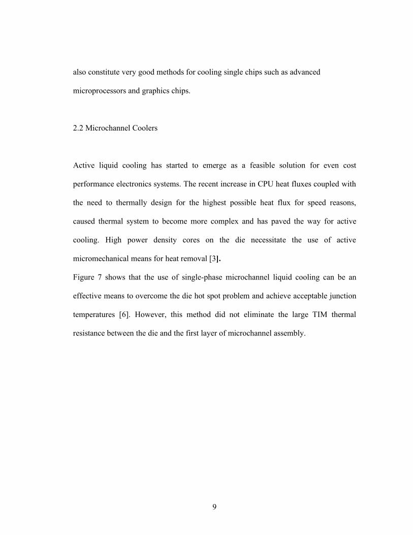
Figure 7 shows that the use of single-phase microchannel liquid cooling can be an
effective means to overcome the die hot spot problem and achieve acceptable junction
temperatures [6]. However, this method did not eliminate the large TIM thermal
resistance between the die and the first layer of microchannel assembly.
10
Figure 7: Hot spot cooling by microchannel liquid cooled plate mounted on chip
substrate via TIM layer [6]
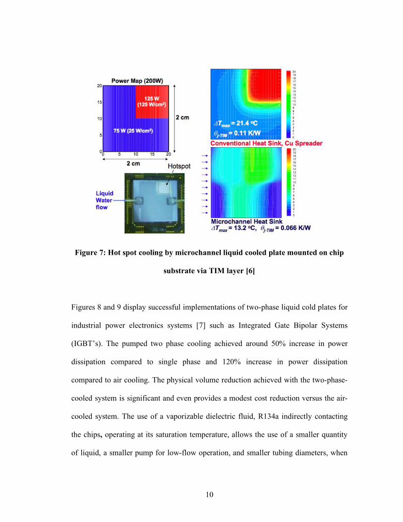
Figures 8 and 9 display successful implementations of two-phase liquid cold plates for
industrial power electronics systems [7] such as Integrated Gate Bipolar Systems
(IGBT’s). The pumped two phase cooling achieved around 50% increase in power
dissipation compared to single phase and 120% increase in power dissipation
compared to air cooling. The physical volume reduction achieved with the two-phase-
cooled system is significant and even provides a modest cost reduction versus the air-
cooled system. The use of a vaporizable dielectric fluid, R134a indirectly contacting
the chips, operating at its saturation temperature, allows the use of a smaller quantity
of liquid, a smaller pump for low-flow operation, and smaller tubing diameters, when

11
compared to a comparable single-phase water cooling system designed for use within
the same type of cabinet (shown in Figure 10) and to dissipate the same module heat
loads. The use of a vaporizable dielectric fluid in a copper cold plate with convoluted
fin internal structure is demonstrated to yield around 100% additional capacity to
dissipate heat generated at the IGBT module base, as compared to the water-cooled
cold plate tested; the improvement over the production air-cooled finned aluminum
extruded thermal solution is demonstrated to be greater than 125% [7].
Figure 8: High Power IGBT Module [7].
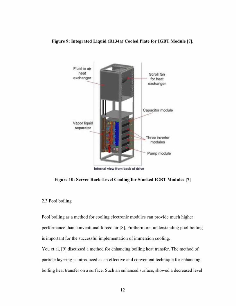
12
Figure 9: Integrated Liquid (R134a) Cooled Plate for IGBT Module [7].
Figure 10: Server Rack-Level Cooling for Stacked IGBT Modules [7]
2.3 Pool boiling
Pool boiling as a method for cooling electronic modules can provide much higher
performance than conventional forced air [8], Furthermore, understanding pool boiling
is important for the successful implementation of immersion cooling.
You et al, [9] discussed a method for enhancing boiling heat transfer. The method of
particle layering is introduced as an effective and convenient technique for enhancing
boiling heat transfer on a surface. Such an enhanced surface, showed a decreased level
13
of wall superheat under boiling and an increased critical heat flux relative to superheat
and critical heat flux values for an untreated surface, due perhaps to an increased
number of nucleation sites or to a change in cooling modalities to two-phase flow in a
porous layer. Application of this technique results in a decrease of heated surface
temperature and a more uniform temperature of the heated surface; both effects are
important in immersion cooling of electronic equipment.
Arik and Bar-Cohen [8], showed that boiling heat transfer with the candidate liquids
provides heat transfer coefficients that are as much as two orders of magnitude higher
than achievable with forced convection of air. Unfortunately, the highly effective
nucleate boiling domain terminates at the Critical Heat Flux, approximately in the
range of 20 W/cm2 at atmospheric conditions and saturation temperature.
Consequently, if immersion cooling is to be used, ways must be found to increase the
pool boiling CHF of these dielectric liquids. Use of a pool boiling CHF correlation
points to the possibility of reaching a CHF of nearly 60 W/cm2, using elevated
pressure and subcooling, along with a dilute mixture of a high boiling point
fluorocarbon, and applying a microporous coating to the surface of the chip.
Bergles and Kim [10], demonstrates that the generation of vapor below a heated
surface is an effective means of reducing the large superheat required for inception of
boiling with liquids suitable for direct immersion cooling of microelectronic devices.
In the experiments with R-113 and a plain copper heat sink surface, the incipient
boiling superheat was reduced from 33 K to as low as 8 K. With a sintered boiling
surfaces, the incipient boiling superheat was reduced from 22 K to as low as 7 K. A
14
reasonable explanation for the effectiveness of this sparging technique is that the
impacting bubbles activate temporarily dormant cavities that, in turn, activate large
neighboring cavities. The technique appears to be easily adaptable to liquid
encapsulated modules containing arrays of microelectronic devices.
Normington et al [11], demonstrated experimental results related to the use of mixtures
of dielectric liquids to control temperature and overshoot while handling high heat
fluxes. A variety of pure dielectric liquids from Ausimont (boiling points from 81 to
110°C) were evaluated. These liquids are similar to Fluorinert liquids from 3M. Data
have been taken on single pure liquids showing the usual expected substantial
overshoot (26’C average) during the incipience of nucleate boiling. The addition of a
second liquid to modulate the temperature and control the overshoot has been
presented. Various mixtures (20-95% of low boiling point; 580% of high boiling point)
were then tested with some mixtures showing virtually no overshoot (0-6 °C) while
still allowing high total heat fluxes greater than 30 W/cm2. On average, the overshoot
was reduced from 26 to 4°C for a variety of liquid mixtures. Some mixtures allowed
for zero overshoot. The 4°C overshoot was less than the temperature variation across
the chip. The effect of liquid mixtures in reducing overshoot is pronounced only in the
high subcooling case (50°C subcooling); for 10°C subcooling, the effect is
insignificant. The mechanisms of these results are not clear. It is, however, clear that
relatively small amounts of a second liquid can strongly modify the boiling heat
transfer characteristics of the dielectric liquids.
15
2.4 Liquid Immersion Cooling
Liquid immersion cooling represents a potential method for meeting the requirements
for removal of increasingly high heat fluxes from individual chips and from three-
dimensional microelectronic packages. Kraus and Bar-Cohen [12] and Bar-Cohen et al
[13], provide a detailed analysis on Liquid immersion cooling of microelectronic
systems, many researchers investigated various aspects of liquid immersion cooling
focusing on 3D modules. The electronic module’s external surface temperature
(condenser temperature) is a crucial aspect in the success of a liquid immersion
technique as it limits the ability of the module’s surface to expel thermal energy
outside the system.
Yokouchi et al [14], presents a cooling techniques using direct immersion cooling for
high-density packaging and provides a discussion focusing on a) the treatment of
bubbles produced by nucleate boiling and b) the control of coolant composition to
prevent “temperature overshoot” occurring at the boiling point as thermal hysteresis.
Maintaining subcooled boiling (the initial stage of nucleate boiling) up to the
maximum power of the application is a useful technique in high-density packaging of
computers because this technique produces fewer problems than saturated boiling.
Using a coolant that mixes two fluorocarbons having different boiling points at a ratio
of 80%-20% was found to prevent temperature overshoot on the chip surface.
The adoption of direct immersion cooling of microelectronic chips and other devices
16
has been hampered by lack of understanding of, and inability to control, the
temperature overshoot or high wall superheat associated with the inception of nucleate
boiling.
2.5 Liquid Immersion Modules
Ciccio and Thun [15], showed that ebullient cooling with FC-78 refrigerant provided
excellent cooling for an ultra-high density VLSI module mounted in a sealed container
for condenser temperatures between 70F and 90F. They were able to double the
module power density sustainable with conventional (forced air) cooling techniques.
At a time when most chips were dissipating less than 1W, it was possible to maintain a
2W/chip and 15 W/in2 (2.35 W/cm2) while keeping junction temperatures blow 150F.
(65.6 0C)
Lee et al, [16] demonstrated experimentally the capability of liquid-encapsulated
system to cool a multi-chip module (MCM) package. Tests were performed on both
dry (no liquid-filled) and liquid-filled packages. In the liquid-filled situation, either a
pure dielectric liquid or a dielectric liquid mixture was employed. The MCM package
was externally cooled by either free-air or forced-air (1.0 to 2.54 m/s of air flow). Heat
transfer history from single-phase, through nucleate boiling, to film boiling was
documented.
The overall improvement for the liquid-filled package was 2–4 times compared to the
dry package, due to the superior thermal properties of dielectric liquids compared to
air. The maximum power dissipation in the liquid-filled package at 2.54 m/s external
17
airflow was 18 W (based on junction temperature maximum of 125C). In the liquid-
filled package, both the single-phase and boiling heat transfer were enhanced by
varying the external boundary conditions from free-air to forced-air.
The total power dissipation limit in the liquid-filled package is strongly influenced by
the ability to condense the vapor in the package. By changing the boundary conditions
from free-air to forced-air (2.54 m/s), the condenser (top lid) efficiency is raised, thus
raising the maximum power dissipation by 2.5 times. Results also indicated that for
any given external boundary condition, the allowable power dissipation did not vary
much under different liquid conditions: non-degassed liquid, degassed liquid at slightly
above ambient pressure, and degassed liquid at ambient pressure. When the system
was sealed, increasing power in the package created large liquid pressure and raised its
boiling point. The chips remained in the single-phase regime and no boiling occurred.
The paper also studies the effect of coolant mixture of two fluids, D80/HT110
(50/50% by volume). The mixture boiling curve behaved differently than the single-
liquid curve: it had a long path of partial boiling and did not reach film boiling as
junction temperature reached 125C. This particular mixture showed less-efficient
boiling heat transfer than the single liquid. However, a proper composition of the
mixture may raise the allowable power in the module compared to the single liquid,
while maintaining the average junction temperature below 125 C. With a small-scale
package (such as in the present study), when the system was sealed (with pure liquid),
increasing power in the package created large liquid pressure and raised its boiling
point. Due to the high boiling point, the dies remained in the single-phase regime.

18
Nelson et al, [17] describes a multi-chip module (MCM) package that uses integral
immersion cooling to transfer heat from the chips to a final heat transfer medium
outside the package. The package is a miniature immersion cooled system with a pin-
fin condenser that can be operated in either the submerged or vapor-space condensing
mode. Tests have been performed with the module fully powered and with subsets of
the chips powered. The results indicate that the heat transfer coefficient is similar in all
partially powered modes. The paper shows that immersion cooling with Fluorinert
FC72 is a viable method of thermally linking the chips in an MCM to an overhead heat
exchanger, competitive in thermal resistance with both through-substrate cooling and
direct above-substrate cooling.
Geisler el al [18], in their paper, explored the viability of passive liquid cooling to
meet the needs of future VME-size electronics modules. Chip heat fluxes in excess of
20W/cm2 were achieved while maintaining chip temperatures below 110°C. Further,
an overall module heat dissipation of 124W was transferred with 80°C module edge
temperatures (FC-72, 3atm, finned module cover). The thermal performance of the
module was limited by the presence of a bubble-fed vapor/air gap that reduced the
ability of the module cover to extract heat from the liquid and threatened to burn out
nearby components as it grew.
2.6 Flow Boiling
Microgap coolers provide direct contact between chemically inert, dielectric fluids and
the back surface of an active electronic component, thus eliminating the significant
19
interface thermal resistance associated with thermal interface materials and/or solid-
solid contact between the component and a microchannel cold plate. On the other hand,
the very good thermal performance, represented by the flow boiling, especially with
annular-flow regime, high heat transfer coefficient, makes the concept of microgap
cooler an appealing one for scholars in the thermal packaging community.
Kim et al [19], provided an exploratory study of the thermofluid characteristics of two-
phase microgap coolers flowing FC-72 in asymmetrically and uniformly heated
channels. Taitel and Dukler flow regime mapping methodology suggested that
intermittent and annular flow regimes dominated the behavior of their 110 micron and
500 micron channels. Their data revealed that area-average heat transfer coefficients
between 7.5 kW/m2K and 15.5 kW/m
2K, can be attained for microgap channels of 110
micron and 500 micron respectively. Heat transfer coefficient data was well bounded
by the predictions of the Chen and Shah correlations for the Annular and Intermittent
flow regimes, respectively.
Rahim et al [20], provided detailed analysis of microchannel/microgap heat transfer
data for two-phase flow of refrigerants and dielectric liquids, gathered from the open
literature and sorted by the Taitel and Dukler flow regime mapping methodology.
Annular flow regime was found to be the dominant regime for this thermal transport
configuration and its prevalence is seen to grow with decreasing channel diameter and
to become dominant for refrigerant flow in channels below 0.1 mm diameter. A
characteristic M-shaped heat transfer coefficient variation with quality (or superficial
velocity) for the flow of refrigerants and dielectric liquids in miniature channels has
20
been identified. Comparison of the microgap refrigerant data to existing classical
correlations reveals that the Chen correlation provides overall agreement to within a
standard deviation of 38% for the entire data set. However, classification of the data by
flow regime does allow for improved predictive accuracy.
Microgap channel coolers flowing two-phase dielectric fluid have a good potential for
cooling advanced high power electronics for they provide good thermal performance
and eliminate the inherited TIM thermal resistance prevailing with indirect liquid
cooling techniques. They also can be considered as cost effective and reliable
technique compared to the expensive microchannel coolers. In order, however, to
address the particular applications in the industry for such microgap channel coolers, a
focus should be on detailed study of the two-phase performance characteristics under
non-ideal conditions including short channel length, non-uniformly heated channels,
conjugate heat transfer effect and packaging in a chip-scale form factor. The present
work focuses on studying and modeling the two-phase characteristics of microgap
channels under these practical non-ideal industry parameters.
21
Chapter 3:
Theoretical Background
3.1 Single-phase Thermofluid Characteristics in miniature channels
The concept of a microgap is a promising cooling technique for advanced
microelectronics. Microgap channels require no thermal interface attachments and thus
allow for the direct and efficient of transfer heat directly form the chip surface. An
appropriate design of a microgap requires knowing the pressure drop and overall
thermal performance, as these two engineering parameters are important to size up the
microgap and the pumping power associated with it.
3.1.1. Pressure drop correlations
Thome [21], in his Wolverine’s Engineering Data Book lists numerous literature
correlations of single-phase pressure drop. Garimella and Singhal [22], showed that
conventional correlations for laminar and turbulent flow adequately predict the
behavior in microchannels of hydraulic diameters as small as 250 µm.
Classical single-phase flow correlations for the pressure drop in parallel plate channel
by Kays and London [23] can be expressed as:
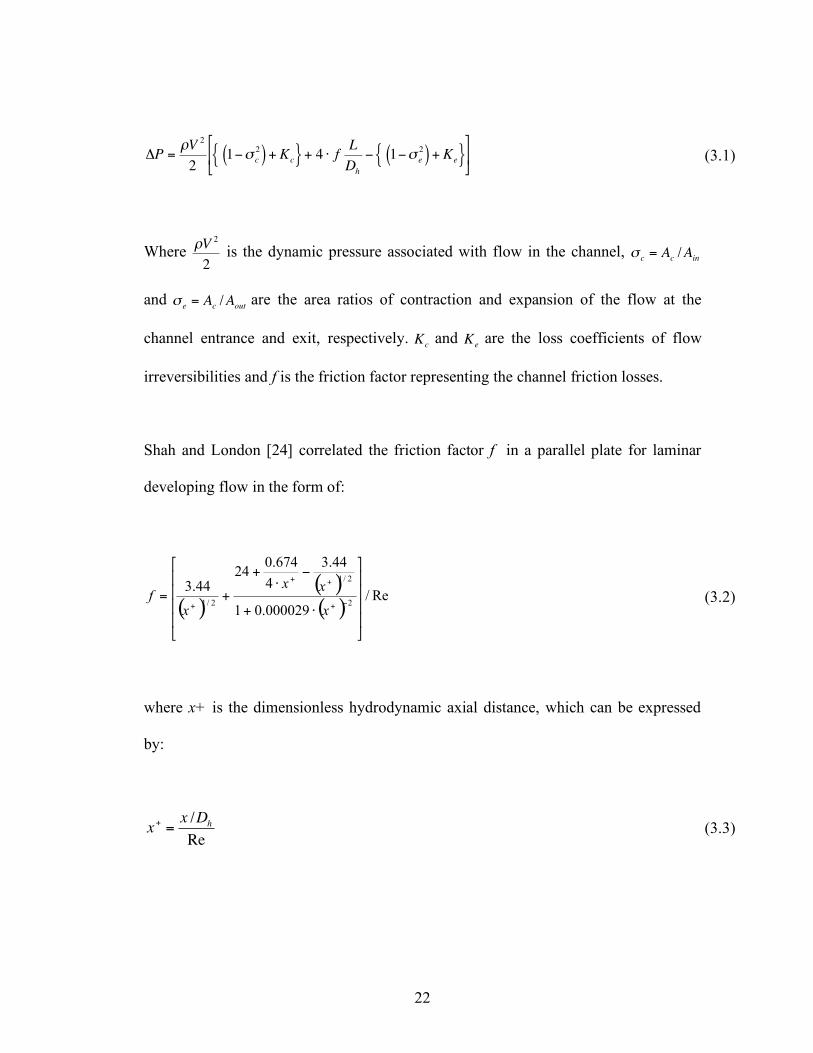
22
!
"P =#V 2
21$% c
2( ) + Kc{ } + 4 & fL
Dh
$ 1$% e
2( ) + Ke{ }'
( )
*
+ , (3.1)
Where
!
"V 2
2
is the dynamic pressure associated with flow in the channel,
!
"c
= Ac/A
in
and
!
"e
= Ac/A
out are the area ratios of contraction and expansion of the flow at the
channel entrance and exit, respectively.
!
Kc and
!
Ke are the loss coefficients of flow
irreversibilities and f is the friction factor representing the channel friction losses.
Shah and London [24] correlated the friction factor f in a parallel plate for laminar
developing flow in the form of:
( )( )( )
Re/
000029.01
44.3
4
674.024
44.3
2
2/1
2/1
!!!!
"
#
$$$$
%
&
'+
('
+
+=(+
++
+ x
xx
xf (3.2)
where x+ is the dimensionless hydrodynamic axial distance, which can be expressed
by:
!
x+
=x /D
h
Re (3.3)
23
In the fully developed laminar flow, i.e. for x+> 0.05, the friction factor reaches an
asymptotic value or f = 96/Re.
3.1.2. Heat transfer correlations
The thermal performance of a microgap channel is evaluated using the dimensionless
Nusslet number as given by:
!
Nu =h.D
h
k (3.4)
Where h is the heat transfer coefficient,
!
Dh is the channel hydraulic diameter and k is
the fluid thermal conductivity and h is the heat transfer coefficient. The heat transfer
coefficient is defined as:
!
h =q
A"T (3.5)
Where
!
"T is the temperature difference between the channel heated surface (wall) and
the cooling fluid, A is the wall surface area and q is the wall heat transfer rate that can
be determined from implementing the channel energy balance equation via:
(3.6)
24
!
q = m•
Cp (Toutlet "Tinlet )
Where
!
m
•
the channel fluid mass flow rate,
!
Cp is the fluid specific heat and
!
Tinlet
and
!
Toutlet
are the channel fluid inlet and outlet temperatures, respectively.
Wolverine’s Engineering Data Book [21], lists numerous literature correlations of
single-phase Nusslet number for a variety of flow types including laminar and fully
developed turbulent flow.
Garimella and Singhal [22], showed that conventional correlations for fluid flow and
heat transfer adequately predict the behavior in microchannels of hydraulic diameters
as small as 250 µm.
Kays and Crawford [25], reviewed many Nusslet number equations available in the
literature for circular tubes, circular tube annuli and rectangular tubes for laminar flow
and thermally fully developed or developing flow with uniform surface temperature
and uniform surface heat flux boundary conditions. Among them, and more directly
related to the channel conditions in the present study, is the Nusslet number for
laminar developing flow in parallel plate channels with isoflux boundary conditions as
!
Nu = 8.24 +0.065(D
h/L)RePr
1+ 0.04[(Dh/L)RePr]
2
3
(3.7)
25
where the value of 8.24 represents Nusslet number for the fully developed laminar
flow.
In the fully developed turbulent flow, Dittus and Boelter equation [25] can be used for
Re>10,000 and is given by
!
Nu = 0.023Re0.8Pr
0.4 (3.8)
More specifically related to the characteristics of the channel type considered in the
present work, Kakac and Shah [26] predicted the local and mean heat transfer
coefficients in uniform heat flux, asymmetrically-heated, parallel plate channels as
follows:
( ) 1
122
*224exp
6
1!
"
=
#$
%&'
( !!= )n
x
n
xnNu
*
* (3.9)
( ) 1
122
*224exp1
6
1!
"
=
#$
%&'
( !!!= )n
m
n
xnNu
*
* (3.10)
Where the dimensionless axial distance is given by:
26
PrRe
/* hDL
x = (3.11)
3.1.3 Effect of heating non-uniformity
It is important to note the lack of available literature and correlations for non-uniform
heat flux in refrigerant-cooled in micro channels. Remley, et al [27], experimentally
investigated turbulent wall friction and forced convection heat transfer in a water-
cooled trapezoidal channel with high Reynolds numbers and 1.14 cm hydraulic
diameter. The paper reported that the Colebrook correlation [25] predicted the
unheated channel friction factors well. It, however, systematically over predicted the
measured friction factors obtained with the test section non-uniformly heated test
section. Perimeter-average convective heat transfer coefficients for laterally non-
uniform imposed heat fluxes were compared with the predictions of three widely-used
correlations for turbulent flow in circular channels. All the correlations under predicted
the data, typically by 11–28%. Although the form factor in Remley, et al’s study is
larger than in the present study, the paper nonetheless discussed an important factor
that is the effect of heating non uniformity on the accuracy of correlations in predicting
pressure drop and thermal performance of studied channels.
3.2 Two-phase Thermofluid Characteristics in miniature channels
3.2.1 Introduction
27
The research community had classified micro channels under different categories with
different definitions. Mehendale et al [28], proposed a purely geometric definition,
ignoring any impact of fluid properties, and considered passages in the diameter range
from 1 micron to 100 micron as micro-channels, 100 microns to 1 mm as meso-channels,
1 mm to 6 mm as compact passages, and greater than 6 mm as conventional passages.
Kandlikar and Grande [29], classified micro channels based on fabrication technology.
They proposed that channels with hydraulic diameters of 3 mm or larger be considered as
conventional, channels with a hydraulic diameter range of 200 micron to 3 mm to be
classified as mini-channels, and, as new technologies were needed to create passages with
diameters below 200 micron, such channels would be defined as micro-channels.
Considering that severe rarefaction effects for many gases are encountered between 10
micron and 0.1 micron, and that such effects might become pronounced in two-phase
flow, Kandlikar and Grande referred to this as the transitional region and used 10
microns as the lower limit on micro-channel behavior.
Kew & Cornwell [30] used the so-called confinement number, defined as the ratio of the
theoretical departing bubble diameter to the channel diameter, i.e.,
!
Co =[" /(g(#l $ #v ))]
d (3.12)
to define the transition to micro-channels flow. Based on a statistical analysis of two
phase heat transfer coefficient data and comparison to correlations provided by Liu and
28
Winterton [31], Cooper [32,33], Lazarek and Black [34], and Tran et al [35], Kew and
Cornwell determined that, for confinement numbers greater than 0.5, the measured heat
transfer coefficients departed significantly from the values predicted by the relevant
conventional channel correlations. They thus chose Co= 0.5 as the transition criteria for
micro-channel behavior. It is interesting to note that, in the present study, the confinement
number Co takes the values of 4.6, 2.3 and 0.93 (all higher than 0.5) for HFE-7100 with
100-, 200- and 500-micron channels, respectively.
Forced flow of dielectric liquids with phase change in heated microgap channels had
been recently the subject of many researches especially in the chemical, nuclear and
mechanical engineering fields. Although the present study focuses the thermal
characteristics of a chip-scale non-ideal and very short uniformly heated microgap
channel with dielectric fluid HFE-7100, it is nonetheless, worth summarizing some of
the available research data on similar refrigerants, flow or geometry parameters. Lee
and Lee [36], investigated two-phase heat transfer in a 300mm long and 20mm wide
horizontal rectangular gap with hydraulic diameters of 0.8mm-3.6mm using R113
refrigerant. They reported the dominance of the annular flow regime and gathered 491
heat transfer coefficient data points in the range of 5 kW/m2K for a mass flux range of
52-208 Kg/m2.s with total pressure drop of 40 kPa. Yang and Fujita [37] used R113 in
a similar but somewhat shorter, 100mm long and 20mm wide horizontal rectangular
gap with hydraulic diameter of 0.4 mm-3.6 mm. Their 292 data points reported heat
transfer coefficients of up to 6 kW/m2K for mass fluxes in the range of 100 Kg/m
2s
29
subject to a heat flux of 2 W/cm2 heat flux. Cortina-Diaz and Schmidt [38]
investigated flow boiling heat transfer using n-Hexane and n-Octane in a 12.7mm by
0.3 mm channel with 0.6 mm hydraulic diameter. They reported heat transfer
coefficient of 6 kW/m2K in the range of a 100 Kg/m
2s mass flux and 2-4 W/cm
2 heat
flux.
Madrid et al. [39] explored the behavior of HFE-7100 in a 40 parallel channel vertical
rectangular channel mini cooler. The channels were 220mm long with a 0.84mm
hydraulic diameter. Their 258 data points indicated a highest heat transfer coefficient
value of 5.7 kW/m2K at 71-191 Kg/m
2s mass flux range and 0.17-0.46 W/cm
2 heat
flux range. A common conclusion from these studies is the heat transfer coefficient
limit of around 6 kW/m2K at the range of 50-200 Kg/m
2s mass flux and subject to low
heat flux of 1-2 W/cm2. The present study focuses on a larger range of mass fluxes of
up to 1500 kg/m2s and heat fluxes up to 50 W/cm
2.
3.2.2. Two-phase flow regime modeling
The flow of two-phase (vapor and liquid) mixture in pipes or channels has special
characteristics and can take different forms, i.e., flow regimes, depending on the distinct
vapor/liquid distributions. Four primary two-phase flow regimes, namely, Bubble,
Intermittent, Stratified and Annular, as well as numerous sub-regimes, have been
identified in the literature [20]. Bubble flow is associated with uniform distribution of
small spherical bubbles within the liquid phase. Intermittent flow is characterized by the
flow of liquid plugs separated by elongated slug-shape gas bubbles. Stratified flow is
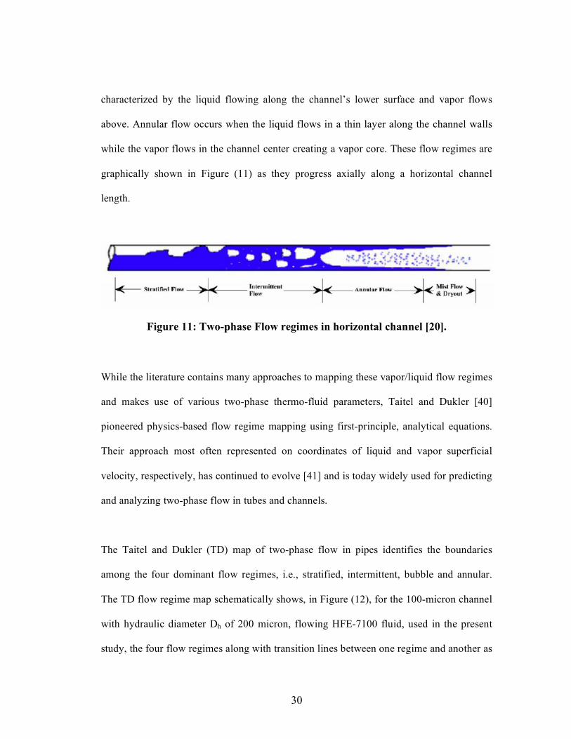
30
characterized by the liquid flowing along the channel’s lower surface and vapor flows
above. Annular flow occurs when the liquid flows in a thin layer along the channel walls
while the vapor flows in the channel center creating a vapor core. These flow regimes are
graphically shown in Figure (11) as they progress axially along a horizontal channel
length.
Figure 11: Two-phase Flow regimes in horizontal channel [20].
While the literature contains many approaches to mapping these vapor/liquid flow regimes
and makes use of various two-phase thermo-fluid parameters, Taitel and Dukler [40]
pioneered physics-based flow regime mapping using first-principle, analytical equations.
Their approach most often represented on coordinates of liquid and vapor superficial
velocity, respectively, has continued to evolve [41] and is today widely used for predicting
and analyzing two-phase flow in tubes and channels.
The Taitel and Dukler (TD) map of two-phase flow in pipes identifies the boundaries
among the four dominant flow regimes, i.e., stratified, intermittent, bubble and annular.
The TD flow regime map schematically shows, in Figure (12), for the 100-micron channel
with hydraulic diameter Dh of 200 micron, flowing HFE-7100 fluid, used in the present
study, the four flow regimes along with transition lines between one regime and another as
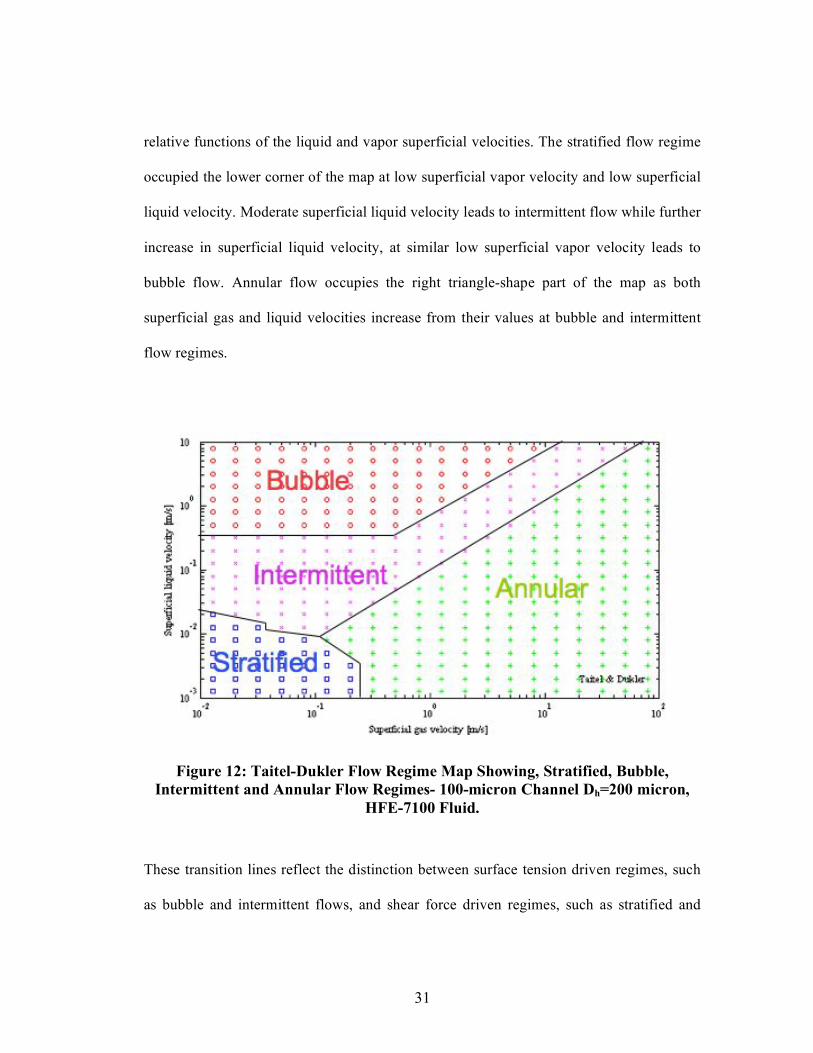
31
relative functions of the liquid and vapor superficial velocities. The stratified flow regime
occupied the lower corner of the map at low superficial vapor velocity and low superficial
liquid velocity. Moderate superficial liquid velocity leads to intermittent flow while further
increase in superficial liquid velocity, at similar low superficial vapor velocity leads to
bubble flow. Annular flow occupies the right triangle-shape part of the map as both
superficial gas and liquid velocities increase from their values at bubble and intermittent
flow regimes.
Figure 12: Taitel-Dukler Flow Regime Map Showing, Stratified, Bubble,
Intermittent and Annular Flow Regimes- 100-micron Channel Dh=200 micron,
HFE-7100 Fluid.
These transition lines reflect the distinction between surface tension driven regimes, such
as bubble and intermittent flows, and shear force driven regimes, such as stratified and
32
annular. Furthermore, the TD flow regime map relies on adiabatic models that ignore the
thermal interactions between phases, the pipe and the environment all of which are present
in the diabatic systems. This dependence of adiabatic models makes the transition lines of
the TD model less accurate when high heat fluxes are applied at the channel/pipe wall
[42].
In addition to the TD flow regime map, other analytical approaches of flow regime
transitions are available in the literature. Amongst them are the Weismann et al method
[43], and Tabatabai and Faghri method [44] that proposed a modification to the TD map
based on a criterion for the transition from surface tension dominated behavior to shear
dominated behavior. These approaches compliment the traditional empirical flow regime
maps obtained for water-steam, and other industrial fluids and cannot be easily
extrapolated to microchannels and refrigerants.
Rahim and Bar-Cohen [20] conducted a detailed analysis of microchannel and microgap
heat transfer data for two-phase flow of refrigerants and dielectric liquids, gathered from
the open literature and sorted by the Taitel and Dukler flow regime mapping methodology,
reveals the existence of the three primary flow regimes, i.e. Bubble, Intermittent, and
Annular, along with Stratified flow for horizontal configurations, in miniature channels.
However, the annular flow regime is found to be the dominant regime for this thermal
transport configuration and its prevalence is seen to grow with decreasing channel
diameter and to become dominant for refrigerant flow in channels below 0.1mm diameter.
33
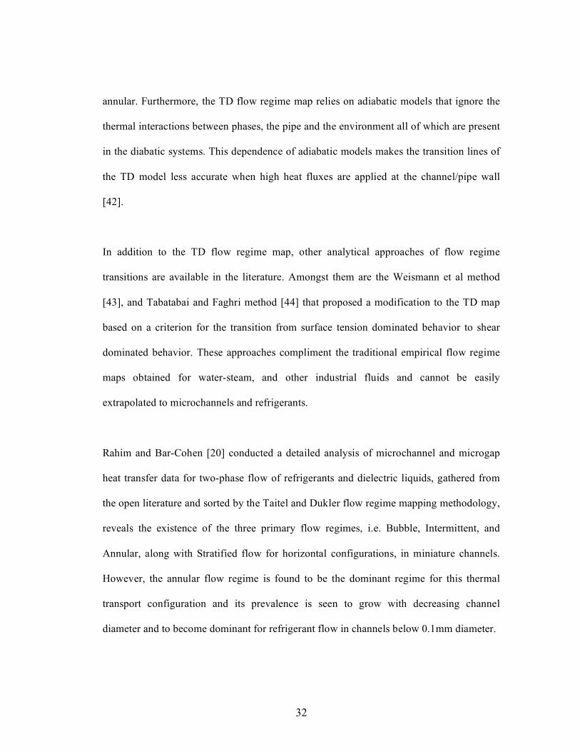
3.2.3. Characteristics of two-phase heat transfer in micro channels
The literature data of two-phase heat transfer coefficients suggest a characteristic M-
shaped heat transfer coefficient variation with quality (or superficial velocity) for the
flow of refrigerants and dielectric liquids in miniature channels. The inflection points
in this M-shaped curve are seen to equate approximately with flow regime transitions,
including a first maximum at the transition from Bubble to Intermittent flow and a
second maximum at moderate qualities in Annular flow, just before local dryout
begins. This characteristic behavior is shown in Figure 13, taken from the
comprehensive work done by Rahim et al [20], on the data from Yang and Fujita [37]
and Cortina-Diaz and Schmidt [38].
Figure 13: Heat transfer coefficient data from Yang and Fujita [37] and Cortina-
Diaz and Schmidt [38] showing the characteristic M-shape behavior [20].
34
3.2.4. Heat Transfer Correlations
Thome and Collier, in their book [45], discussed the classical two-phase heat transfer
correlations available in the literature and identified the prominent role played by the
two-phase Reynolds number, based on the liquid fraction of the mass flux in the
channel, in attempts to correlate the two-phase heat transfer coefficient. Kim, et al [19],
analyzed two-phase microgap heat transfer in simple geometries and correlated to
Chen and Shah correlations. Rahim and Bar-Cohen [20] conducted detailed analysis of
microchannel/microgap heat transfer data for two-phase flow of refrigerants and
dielectric liquids, gathered from the open literature. They analyzed the predictive
accuracy of five classical two-phase heat transfer correlations [45] for miniature
channel flow was examined. These classical correlations include Chen [46], Kandlikar
[47], Gungor-Winterton [48], Gungor-Winterton Revised [49] and Shah correlations
[50]. Selecting the best fitting of the classical correlations for each of the flow regime
categories is seen to yield predictive agreement with regime-sorted heat transfer
coefficients that does not depart significantly from the agreement found in large pipes
and channels.
Comparison of a sample of microgap refrigerant data to existing classical correlations
reveals that the Chen correlation provides overall agreement to within a standard
deviation of 38% for the entire data set [20]. However, classification of the data by
flow regime does allow for improved predictive accuracy. The authors have shown
that the dominant, low quality Annular data could be correlated by the Chen

35
correlation to within an average discrepancy of just 24%, while the Shah correlation
provides agreement to within an average discrepancy of 32% (vs. 72% for Chen) for
data in the Intermittent regime, and the modified Gungor-Winterton correlation to
approximately 37% (vs. 39% for Chen) for the moderate-quality annular flow data.
In the present work, the two correlations for two-phase flow heat transfer prediction,
namely, the Chen and Shah correlations, were used as reference points to compare
against the various experimental data obtained.
Chen Correlation
The starting point for the Chen correlation is:
!
h = hmic
+ hmac
(3.13)
The macroscopic contribution was calculated using the Dengler Addoms correlation
with a Prandtl number correction factor to generalize the correlation beyond water as
the working fluid.
!
hmac
= hlF X
tt( ) (3.14)
Here F is an acceleration factor and the single phase liquid-only convective coefficient
(hl) is calculated via the Dittus-Boelter equation:
36
4.08.0PrRe023.0ll
l
l
D
kh !
"
#$%
&=
(3.15)
where
( )
l
l
DxG
µ
!=
1Re
(3.16)
The microscopic contribution was calculated using the Forster-Zuber correlation for
pool boiling with an additional correction factor in the form of a suppression factor, S:
( )[ ] ( )[ ] SPTPPTTh
ckh lwsatlsatw
vlvl
lpll
mic
75.024.0
24.024.029.05.0
49.045.079.0
00122.0 !!""#
$
%%&
'=
(µ)
( (3.17)
The suppression factor, S is required to account for the fact that nucleation is more
strongly suppressed when the macroscopic convective effect increases in strength and
the wall superheat diminishes. To calculate this suppression factor, Chen used a
regression analysis of the data to fit S as a function of a two phase Reynolds number
defined as:
!
Re tp = Re l F Xtt( )[ ]1.25
(3.18)
37
Chen originally presented the suppression data in graphical format. However, Collier
[45] found the following empirical fit for the suppression factor (which is used in this
study):
( ) ( )117.16Re1056.225.1Re
!!+= tptp xS (3.19)
Collier, also, provided empirical fits for the F(Xtt) data in the form:
!
F Xtt( ) =1 for X
tt
-1 " 0.1
F Xtt( ) = 2.35 0.213+1
Xtt
#
$ %
&
' (
0.736
for Xtt
-1 > 0.1
(3.20)
The Martinelli parameter
!
Xtt is calculated as:
1.05.09.0
1
!!
"
#
$$
%
&!!"
#$$%
&!"
#$%
& '=
g
l
l
g
ttx
xX
µ
µ
(
( (3.21)
Shah Correlation
In the Shah Correlation the heat transfer coefficient takes the form:
( )lel
s FrBoCofh
h,,==! (3.22)
38
With the relevant dimensionless parameters provided as:
5.08.0
1
!!"
#$$%
&!"
#$%
& '=
l
v
x
xCo
(
( (3.23)
lvGh
qBo
"
= (3.24)
gD
GFr
l
le 2
2
!=
(3.25)
The original Shah correlation was presented in graphical form. In 1982 Shah provided
a computational representation of his correlation. This computational representation
was outlined as follows:
04.0Frfor le!=CoN
s (3.26)
04.0Frfor 038.0le
3.0<=
!CoFrN
les (3.27)
4-11EBofor 7.14 !=sF (3.28)
4-11EBofor 4.15 <=sF (3.29)
39
8.08.1
!=
scbN" (3.30)
For Ns > 1
4-0.3E Bofor 2305.0
>= Bonb
! (3.31)
4-0.3E Bofor
4615.0
!
+= Bonb
" (3.32)
( )nbcbs
!!! ,max = (3.33)
For Ns =< 1
( )1 N 0.1for
2.74NexpBo
s
-0.1
s
0.5
!<
=sbsF"
(3.34)
( )1.0 Nfor
2.47NexpBo
s
-0.15
s
0.5
!
=sbsF"
(3.35)
3.2.5 Unresolved issues in two-phase behavior in microgaps
Although there are numerous studies and data on two-phase heat transfer in miniature
and micro channels in the literature, nearly all of these address “ideal” channels, i.e.,
channels that are long enough to produce developed flow and have a uniform heat flux
40
applied along the channel walls. The application of these results and correlations to the
direct cooling of advanced microelectronic chips in non-ideal channels, with non-
uniform heating and relatively short channel lengths, requires dealing with several
unresolved issues.
As discussed in Chapters 1-2, advanced IC’s and especially contemporary
microprocessor architectures experience a high level of transistor modularity that
directly results in non-uniform heating or zonal heating at the die junction (power)
plane. This advancement has resulted in substantial die heating non-uniformity and has
necessitated use of die power (heating) maps to correctly determine the chip
temperature distribution and evaluate the effectiveness of applied thermal management
solutions. . Since the development of the thermal boundary layer in convective heat
transfer and wall ebullition in two-phase flow depend strongly on the local wall heat
flux, it can not be assumed a priori that the available uniform wall heat flux
correlations for the heat transfer coefficients in convection and flow boiling,
respectively, will correctly predict “real” microgap channel behavior. Furthermore, the
focus on miniaturization and compactness in the development of microgap and
microchannel coolers for microelectronic devices results in the design of relatively
short channels with strongly developing flow and significant conductive/convective
conjugate effects in the thermally conductive semi-conductor chips. The available
conventional correlations, with isoflux or isothermal (uniform) boundary conditions
are again inappropriate for predicting the thermofluid behavior of such actual

41
microgap cooler channels. The modeling approached for determining the heat transfer
coefficients prevailing in such channels will be discussed in detail in Chapter 5.
42
Chapter 4:
Experimental Apparatus
4.1 Overall Description
An experiment setup was designed and built for conducting the experimental aspects
of this research. The setup was built around the thermal test chip based on the Intel’s
“Merom” microprocessor [51]. The system was designed to enable flow boiling. An
overall 3-D image of the setup is shown in Figure 14. Schematic layout of the overall
setup is also shown in Figure 15, including the boiling chamber, filling/venting port,
condenser (heat exchanger,) pump, flow meter, inline heater, absolute and differential
pressure transducers and various thermistors including channel (boiling chamber) inlet
and outlet.

43
Figure 14: Two-Phase Microgap Channel Test Apparatus
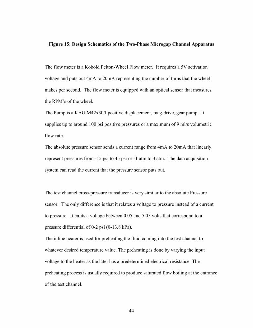
44
Figure 15: Design Schematics of the Two-Phase Microgap Channel Apparatus
The flow meter is a Kobold Pelton-Wheel Flow meter. It requires a 5V activation
voltage and puts out 4mA to 20mA representing the number of turns that the wheel
makes per second. The flow meter is equipped with an optical sensor that measures
the RPM’s of the wheel.
The Pump is a KAG M42x30/I positive displacement, mag-drive, gear pump. It
supplies up to around 100 psi positive pressures or a maximum of 9 ml/s volumetric
flow rate.
The absolute pressure sensor sends a current range from 4mA to 20mA that linearly
represent pressures from -15 psi to 45 psi or -1 atm to 3 atm. The data acquisition
system can read the current that the pressure sensor puts out.
The test channel cross-pressure transducer is very similar to the absolute Pressure
sensor. The only difference is that it relates a voltage to pressure instead of a current
to pressure. It emits a voltage between 0.05 and 5.05 volts that correspond to a
pressure differential of 0-2 psi (0-13.8 kPa).
The inline heater is used for preheating the fluid coming into the test channel to
whatever desired temperature value. The preheating is done by varying the input
voltage to the heater as the later has a predetermined electrical resistance. The
preheating process is usually required to produce saturated flow boiling at the entrance
of the test channel.
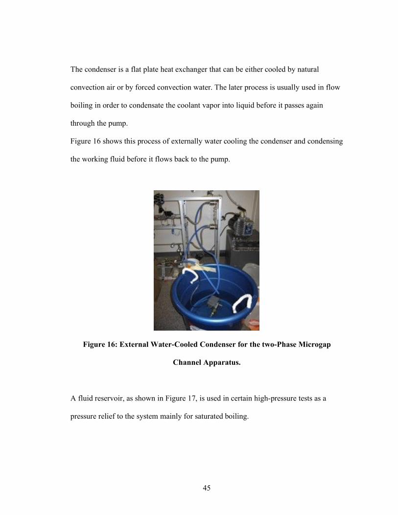
45
The condenser is a flat plate heat exchanger that can be either cooled by natural
convection air or by forced convection water. The later process is usually used in flow
boiling in order to condensate the coolant vapor into liquid before it passes again
through the pump.
Figure 16 shows this process of externally water cooling the condenser and condensing
the working fluid before it flows back to the pump.
Figure 16: External Water-Cooled Condenser for the two-Phase Microgap
Channel Apparatus.
A fluid reservoir, as shown in Figure 17, is used in certain high-pressure tests as a
pressure relief to the system mainly for saturated boiling.
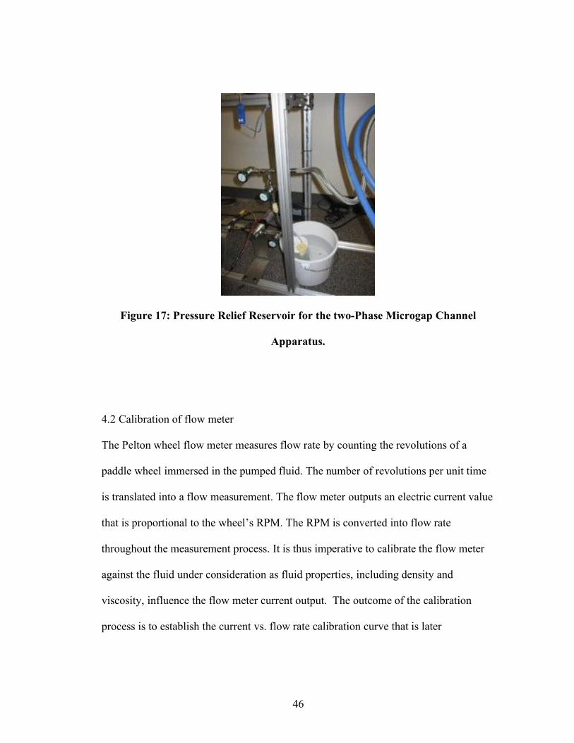
46
Figure 17: Pressure Relief Reservoir for the two-Phase Microgap Channel
Apparatus.
4.2 Calibration of flow meter
The Pelton wheel flow meter measures flow rate by counting the revolutions of a
paddle wheel immersed in the pumped fluid. The number of revolutions per unit time
is translated into a flow measurement. The flow meter outputs an electric current value
that is proportional to the wheel’s RPM. The RPM is converted into flow rate
throughout the measurement process. It is thus imperative to calibrate the flow meter
against the fluid under consideration as fluid properties, including density and
viscosity, influence the flow meter current output. The outcome of the calibration
process is to establish the current vs. flow rate calibration curve that is later
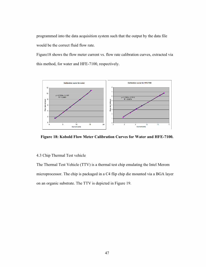
47
programmed into the data acquisition system such that the output by the data file
would be the correct fluid flow rate.
Figure18 shows the flow meter current vs. flow rate calibration curves, extracted via
this method, for water and HFE-7100, respectively.
Figure 18: Kobold Flow Meter Calibration Curves for Water and HFE-7100.
4.3 Chip Thermal Test vehicle
The Thermal Test Vehicle (TTV) is a thermal test chip emulating the Intel Merom
microprocessor. The chip is packaged in a C4 flip chip die mounted via a BGA layer
on an organic substrate. The TTV is depicted in Figure 19.
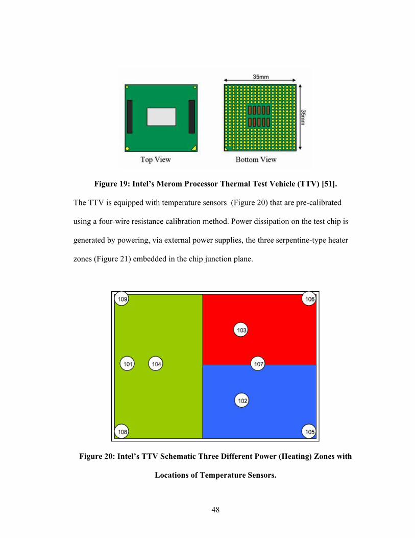
48
Figure 19: Intel’s Merom Processor Thermal Test Vehicle (TTV) [51].
The TTV is equipped with temperature sensors (Figure 20) that are pre-calibrated
using a four-wire resistance calibration method. Power dissipation on the test chip is
generated by powering, via external power supplies, the three serpentine-type heater
zones (Figure 21) embedded in the chip junction plane.
Figure 20: Intel’s TTV Schematic Three Different Power (Heating) Zones with
Locations of Temperature Sensors.

49
Figure 21: Intel’s TTV Serpentine-Type Heating Zones and Locations of
Temperature Sensors [51].
These three zones, superimposed in Figure 22, at the die area, emulate the half-die and
the two quadrants of the microprocessor. The TTV is enabled to run the heater zones
together to produce uniform power dissipation in the plane pf the resistors or the zones
can be run individually or in binary combinations to produce various non-uniform
power dissipation distributions. The heat flux achievable for uniform power dissipation
is 50 W/cm2 and it can rise to 200 W/cm
2 for non-uniform power dissipation where the
full power is concentrated on one quadrant of the chip area.
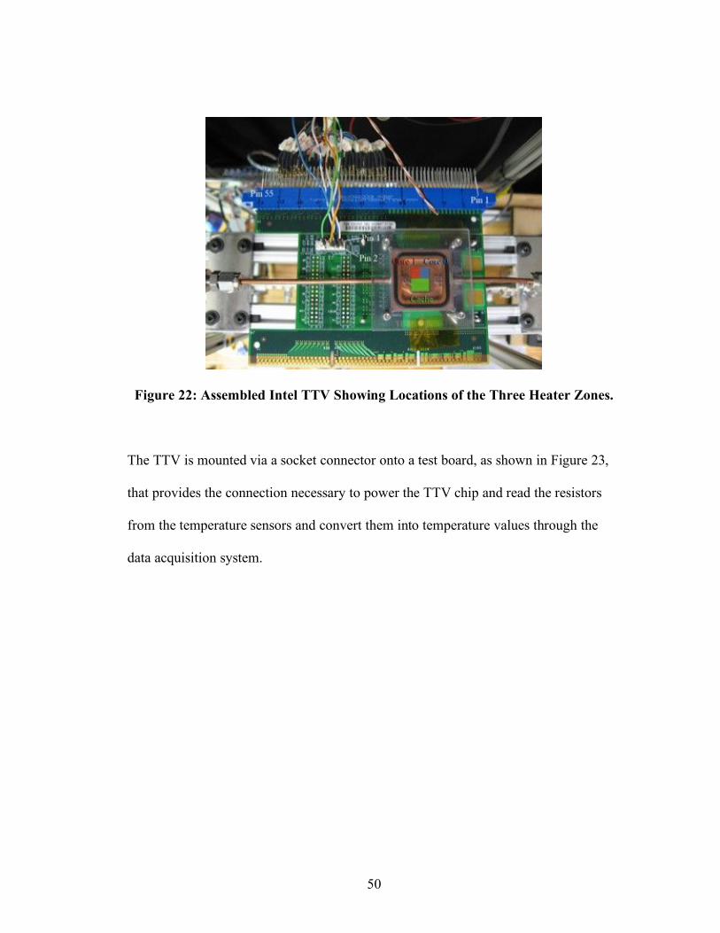
50
Figure 22: Assembled Intel TTV Showing Locations of the Three Heater Zones.
The TTV is mounted via a socket connector onto a test board, as shown in Figure 23,
that provides the connection necessary to power the TTV chip and read the resistors
from the temperature sensors and convert them into temperature values through the
data acquisition system.
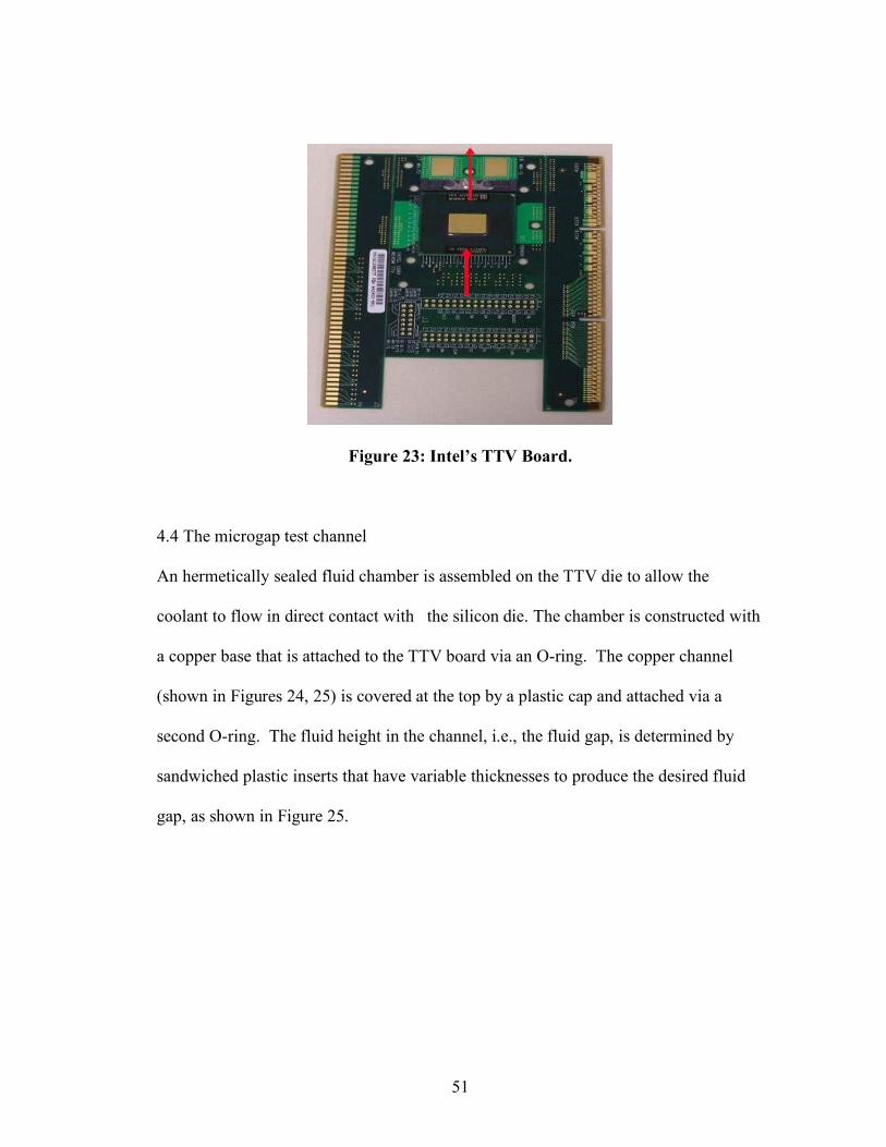
51
Figure 23: Intel’s TTV Board.
4.4 The microgap test channel
An hermetically sealed fluid chamber is assembled on the TTV die to allow the
coolant to flow in direct contact with the silicon die. The chamber is constructed with
a copper base that is attached to the TTV board via an O-ring. The copper channel
(shown in Figures 24, 25) is covered at the top by a plastic cap and attached via a
second O-ring. The fluid height in the channel, i.e., the fluid gap, is determined by
sandwiched plastic inserts that have variable thicknesses to produce the desired fluid
gap, as shown in Figure 25.
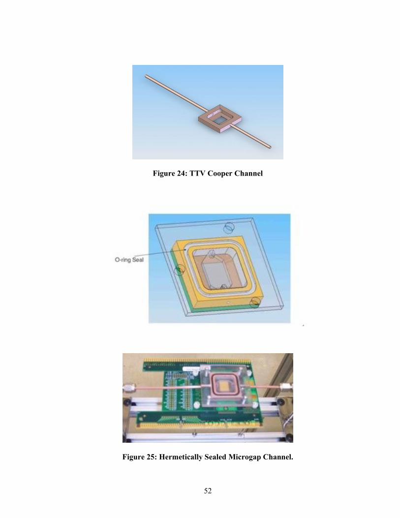
52
Figure 24: TTV Cooper Channel
Figure 25: Hermetically Sealed Microgap Channel.
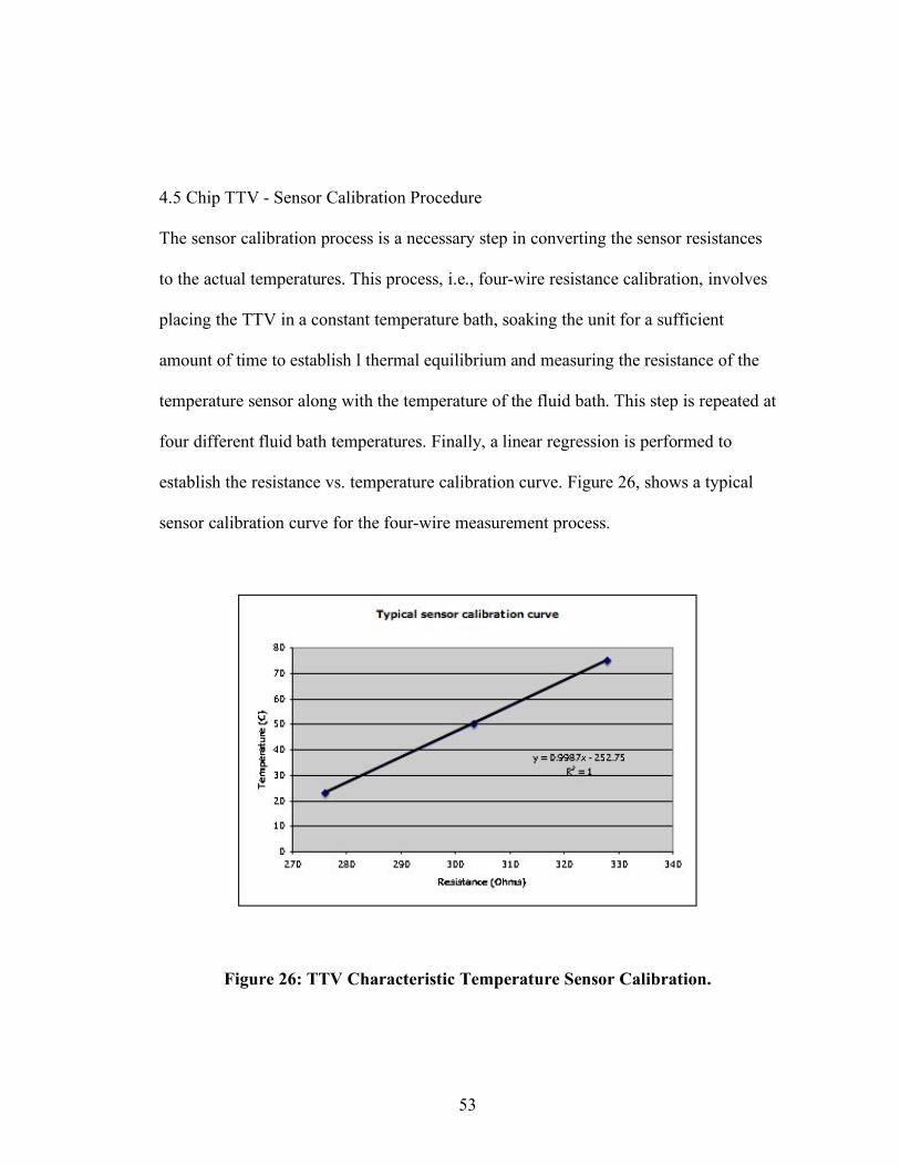
53
4.5 Chip TTV - Sensor Calibration Procedure
The sensor calibration process is a necessary step in converting the sensor resistances
to the actual temperatures. This process, i.e., four-wire resistance calibration, involves
placing the TTV in a constant temperature bath, soaking the unit for a sufficient
amount of time to establish l thermal equilibrium and measuring the resistance of the
temperature sensor along with the temperature of the fluid bath. This step is repeated at
four different fluid bath temperatures. Finally, a linear regression is performed to
establish the resistance vs. temperature calibration curve. Figure 26, shows a typical
sensor calibration curve for the four-wire measurement process.
Figure 26: TTV Characteristic Temperature Sensor Calibration.
54
4.6 Fluid selection and HFE-7100 Novec properties
Water’s thermal characteristics including thermal conductivity, specific heat and latent
heat of vaporization, make it an ideal and the most popular coolant for a wide variety
of thermal management applications. However, water is electrically conductive and
could cause device failure and IC shorting, as well as corrosive actions, if a water-
cooled thermal management component experiences leakage. The industry, therefore,
prefers dielectric fluids for advanced liquid cooling of electronic components.
Historically, the dielectric fluorinerts [52], i.e., the FC family of fluids, along with
other refrigerants (such as R134x, etc.) had been extensively used in liquid cooled
products. These fluids, however, do not possess good environmental properties,
displaying high global warming potential (GWP) and ozone depletion potential (ODP)
[52]. The chemical industry led by 3M pioneered a new family of liquid cooling
products, Novec, aimed at addressing the environmental and toxicity aspects and
characteristics of FC’s. 3M™ Novec™ 7100 Engineered Fluid [52], is used in the
present work. HFE-7100, chemically known as methoxy-nonafluorobutane
(C4F9OCH3), is a clear, colorless and low-odor fluid intended to replace ozone-
depleting substances (ODSs) and compounds with high global warming potential
(GWP). This proprietary fluid has zero ozone depletion potential and other favorable
environmental properties (see Table 1). It has one of the best toxicological profiles
(Table 2) of CFC replacement materials, with a time-weighted average exposure
guideline of 750 ppm (eight hour average). Table 3, shows published properties from
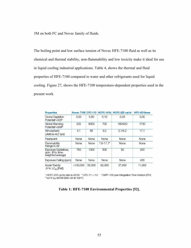
55
3M on both FC and Novec family of fluids.
The boiling point and low surface tension of Novec HFE-7100 fluid as well as its
chemical and thermal stability, non-flammability and low toxicity make it ideal for use
in liquid cooling industrial applications. Table 4, shows the thermal and fluid
properties of HFE-7100 compared to water and other refrigerants used for liquid
cooling. Figure 27, shows the HFE-7100 temperature-dependent properties used in the
present work.
Table 1: HFE-7100 Environmental Properties [52].

56
Table 2: HFE-7100 Toxicity Properties [52].

57
Table 3: Characteristics of 3M’s Fluorinert and Novec Fluids [52].
Property HFE-7100 FC-72 R-134a R-245a Water
Chemical Formula C4F9OCH3 C6F14 C2H2F4 CHF2CH2CF3 H2O
Boiling Point (1atm) [°C] 61 56 -26 14.9 100
Density [kg/m3] 1510 1680 1377 1366 1000
Surface Tension [dyne/cm] 12.3 12 15.3 - 58.9
Kinematic Viscosity [cSt] 0.38 0.38 2.74 3.43 2.87
Latent Heat of Vaporization [kJ/kg] 121.2 88 212.1 197.3 2257
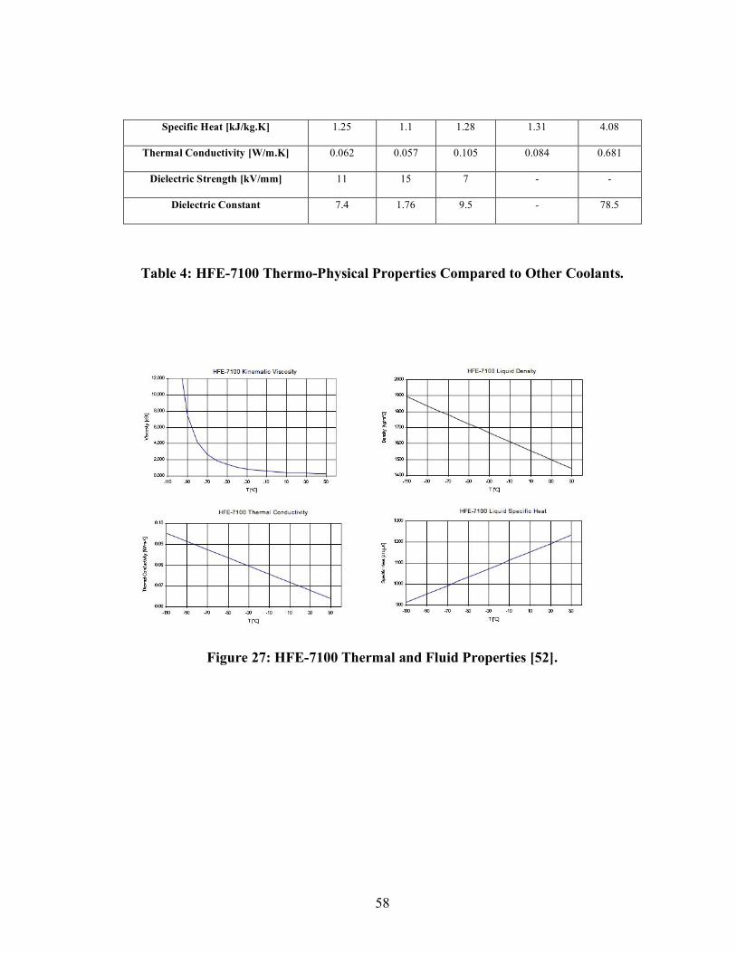
58
Specific Heat [kJ/kg.K] 1.25 1.1 1.28 1.31 4.08
Thermal Conductivity [W/m.K] 0.062 0.057 0.105 0.084 0.681
Dielectric Strength [kV/mm] 11 15 7 - -
Dielectric Constant 7.4 1.76 9.5 - 78.5
Table 4: HFE-7100 Thermo-Physical Properties Compared to Other Coolants.
Figure 27: HFE-7100 Thermal and Fluid Properties [52].
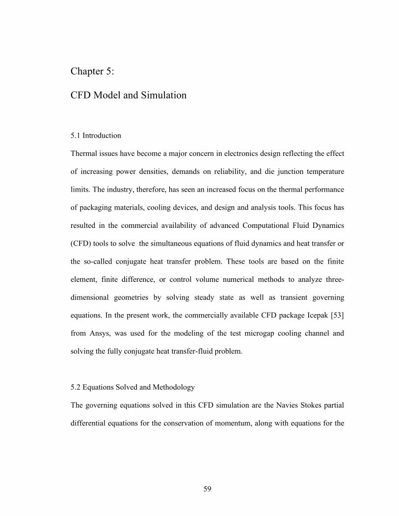
59
Chapter 5:
CFD Model and Simulation
5.1 Introduction
Thermal issues have become a major concern in electronics design reflecting the effect
of increasing power densities, demands on reliability, and die junction temperature
limits. The industry, therefore, has seen an increased focus on the thermal performance
of packaging materials, cooling devices, and design and analysis tools. This focus has
resulted in the commercial availability of advanced Computational Fluid Dynamics
(CFD) tools to solve the simultaneous equations of fluid dynamics and heat transfer or
the so-called conjugate heat transfer problem. These tools are based on the finite
element, finite difference, or control volume numerical methods to analyze three-
dimensional geometries by solving steady state as well as transient governing
equations. In the present work, the commercially available CFD package Icepak [53]
from Ansys, was used for the modeling of the test microgap cooling channel and
solving the fully conjugate heat transfer-fluid problem.
5.2 Equations Solved and Methodology
The governing equations solved in this CFD simulation are the Navies Stokes partial
differential equations for the conservation of momentum, along with equations for the

60
conservation of mass (continuity) and conservation of energy. The three equations take
the following forms
!
" #r u = 0 (5.1)
!
"#r u
#t+ "(
r u $ %)
r u = &%P + "%2
r u + "
r g '(T &T() (5.2)
!
"cp
#T
#t+ "c p
r u $ %T =% $ k%T + S (5.3)
The conjugate flow and heat solution is obtained using the Boussinesq approximation
for buoyancy forces.
!
"g(# " #amb ) = #ambg$(T "T%) (5.4)
Thermal radiation is a non-linear phenomenon and solved for fully by calculating
exchange factors for all surfaces and adding an appropriate term to the energy equation.
!
Q ="#AT 4 (5.5)
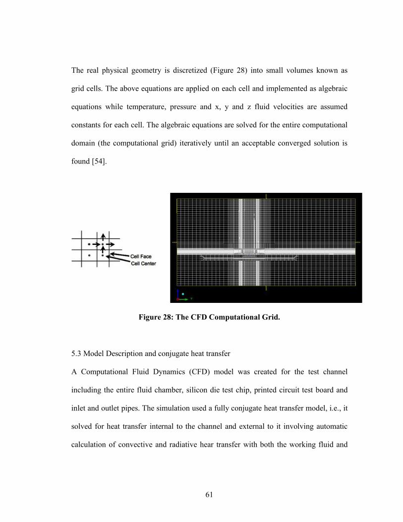
61
The real physical geometry is discretized (Figure 28) into small volumes known as
grid cells. The above equations are applied on each cell and implemented as algebraic
equations while temperature, pressure and x, y and z fluid velocities are assumed
constants for each cell. The algebraic equations are solved for the entire computational
domain (the computational grid) iteratively until an acceptable converged solution is
found [54].
Figure 28: The CFD Computational Grid.
5.3 Model Description and conjugate heat transfer
A Computational Fluid Dynamics (CFD) model was created for the test channel
including the entire fluid chamber, silicon die test chip, printed circuit test board and
inlet and outlet pipes. The simulation used a fully conjugate heat transfer model, i.e., it
solved for heat transfer internal to the channel and external to it involving automatic
calculation of convective and radiative hear transfer with both the working fluid and
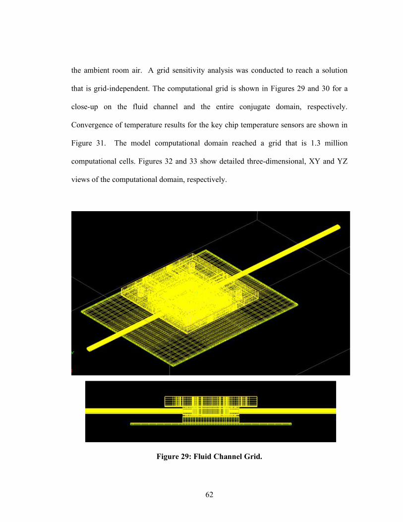
62
the ambient room air. A grid sensitivity analysis was conducted to reach a solution
that is grid-independent. The computational grid is shown in Figures 29 and 30 for a
close-up on the fluid channel and the entire conjugate domain, respectively.
Convergence of temperature results for the key chip temperature sensors are shown in
Figure 31. The model computational domain reached a grid that is 1.3 million
computational cells. Figures 32 and 33 show detailed three-dimensional, XY and YZ
views of the computational domain, respectively.
Figure 29: Fluid Channel Grid.
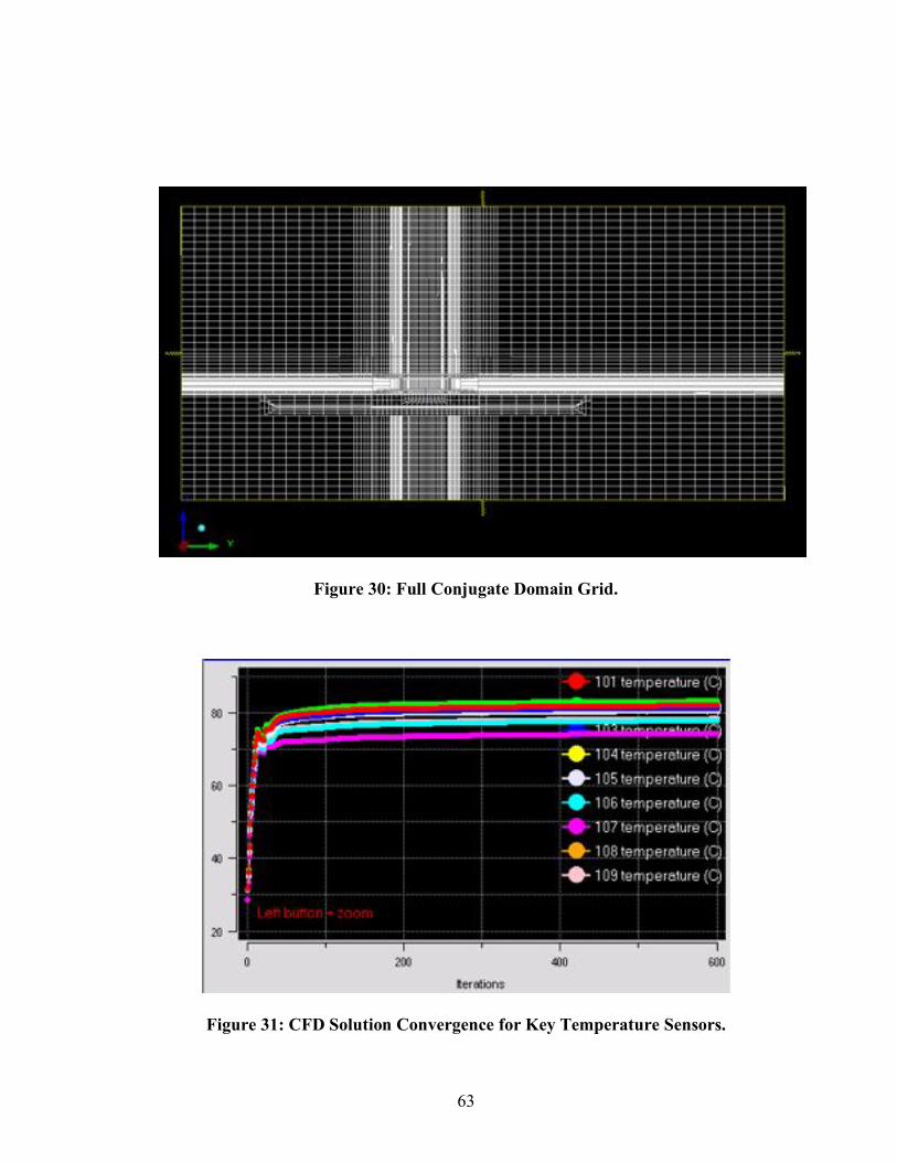
63
Figure 30: Full Conjugate Domain Grid.
Figure 31: CFD Solution Convergence for Key Temperature Sensors.
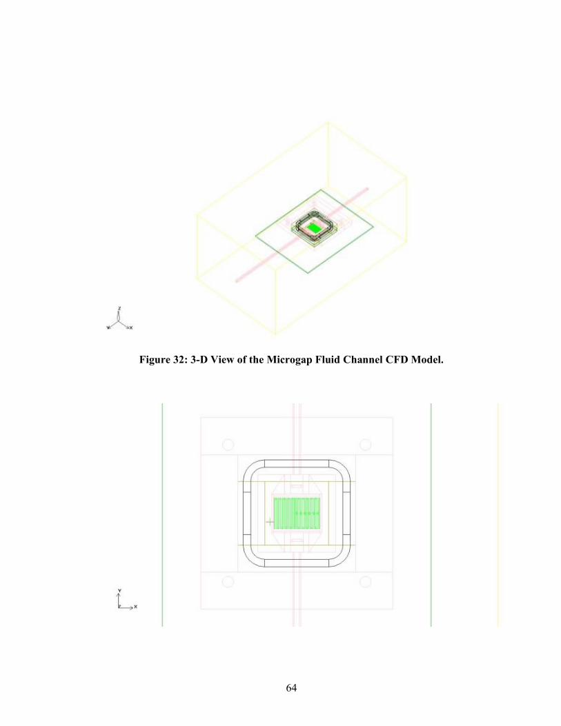
64
Figure 32: 3-D View of the Microgap Fluid Channel CFD Model.
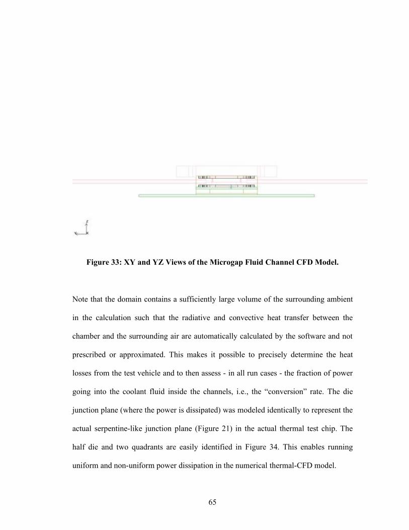
65
Figure 33: XY and YZ Views of the Microgap Fluid Channel CFD Model.
Note that the domain contains a sufficiently large volume of the surrounding ambient
in the calculation such that the radiative and convective heat transfer between the
chamber and the surrounding air are automatically calculated by the software and not
prescribed or approximated. This makes it possible to precisely determine the heat
losses from the test vehicle and to then assess - in all run cases - the fraction of power
going into the coolant fluid inside the channels, i.e., the “conversion” rate. The die
junction plane (where the power is dissipated) was modeled identically to represent the
actual serpentine-like junction plane (Figure 21) in the actual thermal test chip. The
half die and two quadrants are easily identified in Figure 34. This enables running
uniform and non-uniform power dissipation in the numerical thermal-CFD model.
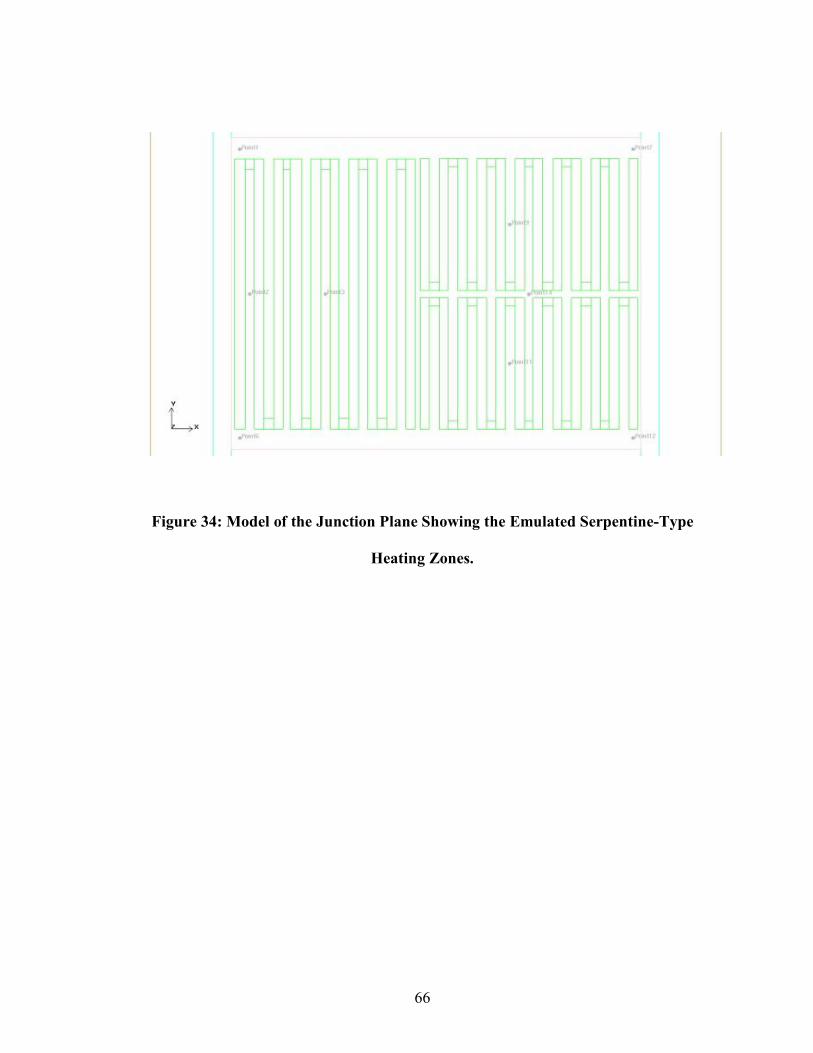
66
Figure 34: Model of the Junction Plane Showing the Emulated Serpentine-Type
Heating Zones.

67
Chapter 6:
Single-Phase Data and Discussion
6.1 Basic relations
The thermal performance of a micro gap (micro channel) is characterized by the
dimensionless Nusslet number (Nu) as given by
!
Nu =hD
h
k (6.1)
Where
!
k is the fluid thermal conductivity,
!
Dh is the gap hydraulic diameter as given
by
!
Dh =4.(cross sec tion area)
wetted perimeter (6.2)
and
!
h is the micro gap heat transfer coefficient. The heat transfer coefficient is given
by
!
h =q
A"T (6.3)
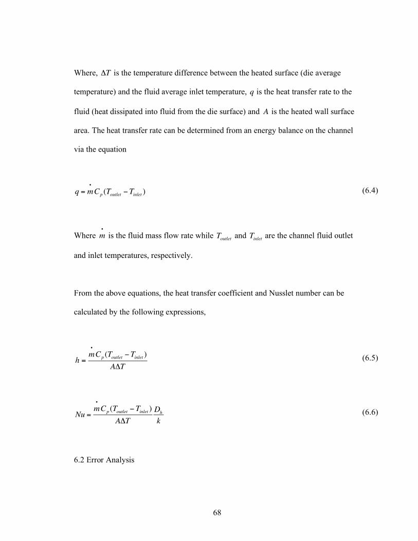
68
Where,
!
"T is the temperature difference between the heated surface (die average
temperature) and the fluid average inlet temperature,
!
q is the heat transfer rate to the
fluid (heat dissipated into fluid from the die surface) and
!
A is the heated wall surface
area. The heat transfer rate can be determined from an energy balance on the channel
via the equation
!
q = m•
Cp (Toutlet "Tinlet ) (6.4)
Where
!
m
•
is the fluid mass flow rate while
!
Toutlet
and
!
Tinlet
are the channel fluid outlet
and inlet temperatures, respectively.
From the above equations, the heat transfer coefficient and Nusslet number can be
calculated by the following expressions,
!
h =m•
Cp (Toutlet "Tinlet )
A#T (6.5)
!
Nu =m•
Cp (Toutlet "Tinlet )
A#T
Dh
k (6.6)
6.2 Error Analysis
69
The test measurement error can be divided into bias errors and precision errors [54].
The bias error remains constant during the measurements under a fixed operating
condition. The bias error can be estimated by calibration, concomitant methodology,
inter-laboratory comparison and experience. When measurements are repeated under
fixed operating conditions, the precision error is affected by the repeatability and
resolution of the equipment used, the temporal and spatial variation of variables, the
variations in measured variables, and variations in operating and environmental
conditions in the measurement processes. Each measurement error would be combined
with other errors in some manner, which increases the uncertainty of the measurement.
A first-order estimate of the uncertainty in the measurement due to the individual
errors can be computed by the root-sum-square method [55].
The uncertainty in the single-phase heat transfer coefficient, obtained from the channel
energy balance equation above, is linear and is affected by the uncertainties in the
measured quantities including the flow rate, the temperature of the wall (die sensors),
the temperature of inlet and outlet, the stability of the data logger and power supply. It
can be expressed mathematically as
!
"h
h
#
$ %
&
' (
2
="m
•
m•
#
$
% %
&
'
( (
2
+"q
q
#
$ %
&
' (
2
+")Twall)Twall
#
$ %
&
' (
2
(6.7)
70
Where
!
" h is the uncertainty of the heat transfer coefficient,
!
"m•
is the error of flow
rate via the flow meter,
!
"q is error of input power via the power supply,
!
"#Twall
is the
measurement error of wall excess temperature. The flow meter’s flow rate error is ±
1.5%. The error of the power supply is ± 2.5%. The maximum error in the wall excess
temperature measurement is ± 0.25°C which causes maximum error of 1%. Thus, the
possible maximum error in measuring the heat transfer coefficient is ±3%.
The uncertainty in the measured pressure drop across the gap (channel) is determined
by the accuracy of the pressure transducer (± 0.25% Full Scale). However, uncertainty
of the measured pressure drop is linearly dependent on the uncertainty in the
measurement of flow. Therefore the resulting uncertainty of measuring pressure drop
can be expressed as
!
"#P
#P
$
% &
'
( )
2
="m
•
m
•
$
%
& &
'
(
) )
2
+"#P
t
#Pt
$
% &
'
( )
2
(6.8)
Where
!
"P is pressure drop and
!
"#P is the uncertainty of pressure drop measurement
and
!
"#Pt is the error of the pressure transducer. The error of pressure transducer is ±
0.25% FS. Therefore, the possible maximum error in the pressure drop measurement is
1.52%.
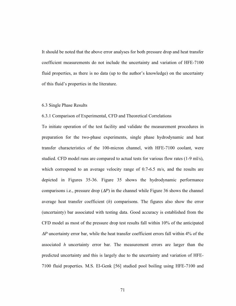
71
It should be noted that the above error analyses for both pressure drop and heat transfer
coefficient measurements do not include the uncertainty and variation of HFE-7100
fluid properties, as there is no data (up to the author’s knowledge) on the uncertainty
of this fluid’s properties in the literature.
6.3 Single Phase Results
6.3.1 Comparison of Experimental, CFD and Theoretical Correlations
To initiate operation of the test facility and validate the measurement procedures in
preparation for the two-phase experiments, single phase hydrodynamic and heat
transfer characteristics of the 100-micron channel, with HFE-7100 coolant, were
studied. CFD model runs are compared to actual tests for various flow rates (1-9 ml/s),
which correspond to an average velocity range of 0.7-6.5 m/s, and the results are
depicted in Figures 35-36. Figure 35 shows the hydrodynamic performance
comparisons i.e., pressure drop (!P) in the channel while Figure 36 shows the channel
average heat transfer coefficient (h) comparisons. The figures also show the error
(uncertainty) bar associated with testing data. Good accuracy is established from the
CFD model as most of the pressure drop test results fall within 10% of the anticipated
!P uncertainty error bar, while the heat transfer coefficient errors fall within 4% of the
associated h uncertainty error bar. The measurement errors are larger than the
predicted uncertainty and this is largely due to the uncertainty and variation of HFE-
7100 fluid properties. M.S. El-Genk [56] studied pool boiling using HFE-7100 and

72
reported correlations errors of 10% larger than the measurement uncertainty of 3.7%.
Similar fluid-properties based errors were reported by Kim et al, [19].
Figure 35: Effect of Fluid Velocity on Single-Phase Pressure Drop in a 100-
micron Microgap Channel Flowing HFE-7100 (Dh = 200 micron).
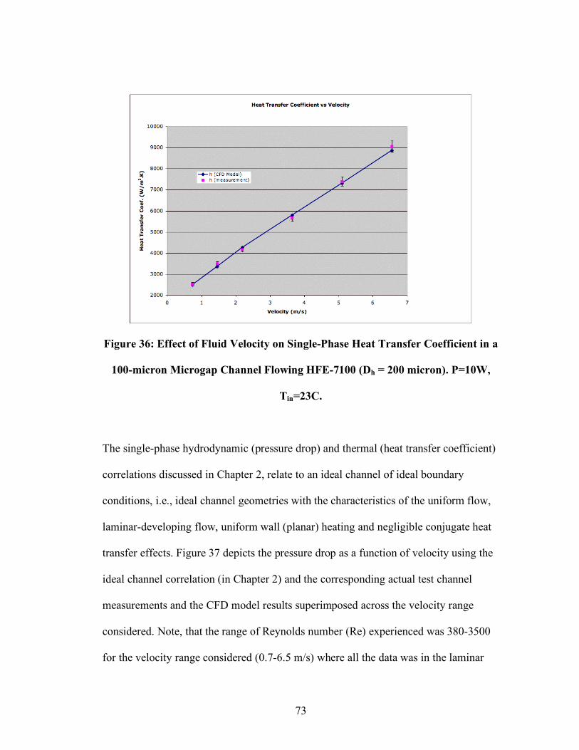
73
Figure 36: Effect of Fluid Velocity on Single-Phase Heat Transfer Coefficient in a
100-micron Microgap Channel Flowing HFE-7100 (Dh = 200 micron). P=10W,
Tin=23C.
The single-phase hydrodynamic (pressure drop) and thermal (heat transfer coefficient)
correlations discussed in Chapter 2, relate to an ideal channel of ideal boundary
conditions, i.e., ideal channel geometries with the characteristics of the uniform flow,
laminar-developing flow, uniform wall (planar) heating and negligible conjugate heat
transfer effects. Figure 37 depicts the pressure drop as a function of velocity using the
ideal channel correlation (in Chapter 2) and the corresponding actual test channel
measurements and the CFD model results superimposed across the velocity range
considered. Note, that the range of Reynolds number (Re) experienced was 380-3500
for the velocity range considered (0.7-6.5 m/s) where all the data was in the laminar
74
flow regime except for the last two data points (at 5 m/s and 6.5 m/s velocities or Re of
2700 and 3500, respectively) where the flow was in the laminar-to-turbulent transition
regime. On the other hand, due to the very short channel considered (10.5 mm in
length), the hydrodynamic entry length - approximately given by
!
0.05.Re.Dh [25] -
was higher than the channel length across the velocity range considered, except for the
very low velocities of 0.7 m/s and 1.5 m/s, for which, the channel experienced a
combination of developing and fully developed flow. The thermal entry length given
by
!
0.05.Re.PrDh [25] was, however, higher than the channel length across the full
velocity range considered and thus the thermal transport in the channel was always in
the developing flow condition.
While CFD results do not agree well with the correlations, they however can simulate
these non-idealities and show good agreement with actual measurements. Using the
ideal channel correlation to predict the actual non-ideal channel measured pressure
drops, provides a similar trend with fluid velocity but yields an average error of 24%
with the largest error at the low velocities. The CFD model, however, provides much
better agreement with measurements whereby the average error is reduced to 5%.
Figure 38 depicts the heat transfer coefficient as a function of flow rate using the ideal
channel correlation and the corresponding actual test channel measured heat transfer
coefficient’s, superimposed across the velocity range considered. Very similar
conclusions, to those of the hydrodynamic ones, can be drawn for the heat transfer
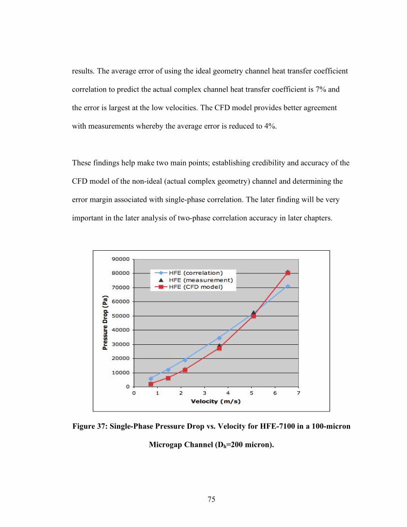
75
results. The average error of using the ideal geometry channel heat transfer coefficient
correlation to predict the actual complex channel heat transfer coefficient is 7% and
the error is largest at the low velocities. The CFD model provides better agreement
with measurements whereby the average error is reduced to 4%.
These findings help make two main points; establishing credibility and accuracy of the
CFD model of the non-ideal (actual complex geometry) channel and determining the
error margin associated with single-phase correlation. The later finding will be very
important in the later analysis of two-phase correlation accuracy in later chapters.
Figure 37: Single-Phase Pressure Drop vs. Velocity for HFE-7100 in a 100-micron
Microgap Channel (Dh=200 micron).
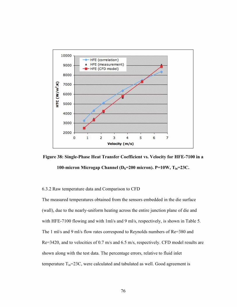
76
Figure 38: Single-Phase Heat Transfer Coefficient vs. Velocity for HFE-7100 in a
100-micron Microgap Channel (Dh=200 micron). P=10W, Tin=23C.
6.3.2 Raw temperature data and Comparison to CFD
The measured temperatures obtained from the sensors embedded in the die surface
(wall), due to the nearly-uniform heating across the entire junction plane of die and
with HFE-7100 flowing and with 1ml/s and 9 ml/s, respectively, is shown in Table 5.
The 1 ml/s and 9 ml/s flow rates correspond to Reynolds numbers of Re=380 and
Re=3420, and to velocities of 0.7 m/s and 6.5 m/s, respectively. CFD model results are
shown along with the test data. The percentage errors, relative to fluid inlet
temperature Tin=23C, were calculated and tabulated as well. Good agreement is
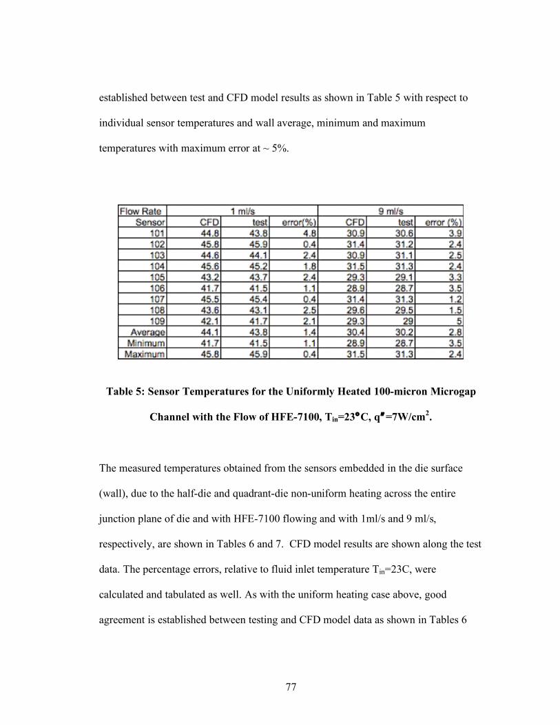
77
established between test and CFD model results as shown in Table 5 with respect to
individual sensor temperatures and wall average, minimum and maximum
temperatures with maximum error at ~ 5%.
Table 5: Sensor Temperatures for the Uniformly Heated 100-micron Microgap
Channel with the Flow of HFE-7100, Tin=23°C, q!=7W/cm2.
The measured temperatures obtained from the sensors embedded in the die surface
(wall), due to the half-die and quadrant-die non-uniform heating across the entire
junction plane of die and with HFE-7100 flowing and with 1ml/s and 9 ml/s,
respectively, are shown in Tables 6 and 7. CFD model results are shown along the test
data. The percentage errors, relative to fluid inlet temperature Tin=23C, were
calculated and tabulated as well. As with the uniform heating case above, good
agreement is established between testing and CFD model data as shown in Tables 6
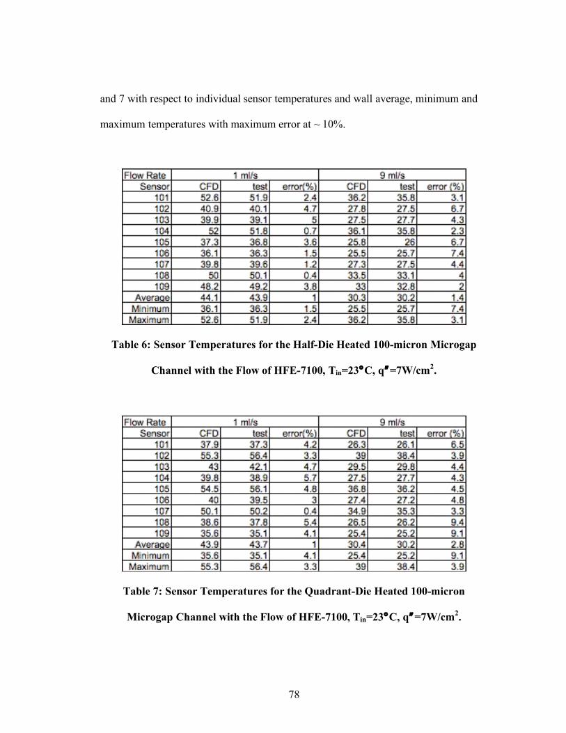
78
and 7 with respect to individual sensor temperatures and wall average, minimum and
maximum temperatures with maximum error at ~ 10%.
Table 6: Sensor Temperatures for the Half-Die Heated 100-micron Microgap
Channel with the Flow of HFE-7100, Tin=23°C, q!=7W/cm2.
Table 7: Sensor Temperatures for the Quadrant-Die Heated 100-micron
Microgap Channel with the Flow of HFE-7100, Tin=23°C, q!=7W/cm2.
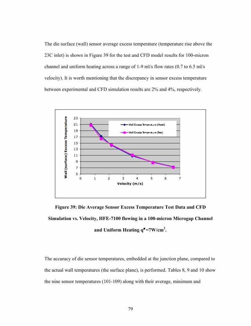
79
The die surface (wall) sensor average excess temperature (temperature rise above the
23C inlet) is shown in Figure 39 for the test and CFD model results for 100-micron
channel and uniform heating across a range of 1-9 ml/s flow rates (0.7 to 6.5 ml/s
velocity). It is worth mentioning that the discrepancy in sensor excess temperature
between experimental and CFD simulation results are 2% and 4%, respectively.
Figure 39: Die Average Sensor Excess Temperature Test Data and CFD
Simulation vs. Velocity, HFE-7100 flowing in a 100-micron Microgap Channel
and Uniform Heating q!=7W/cm2.
The accuracy of die sensor temperatures, embedded at the junction plane, compared to
the actual wall temperatures (the surface plane), is performed. Tables 8, 9 and 10 show
the nine sensor temperatures (101-109) along with their average, minimum and
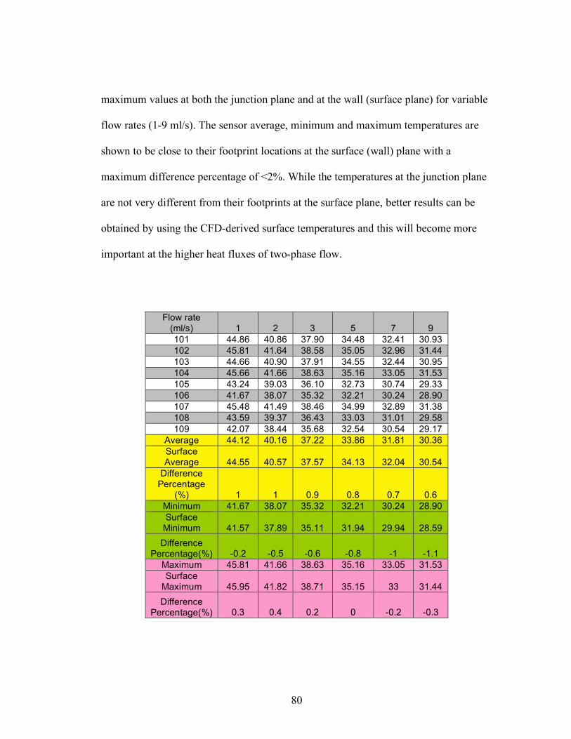
80
maximum values at both the junction plane and at the wall (surface plane) for variable
flow rates (1-9 ml/s). The sensor average, minimum and maximum temperatures are
shown to be close to their footprint locations at the surface (wall) plane with a
maximum difference percentage of <2%. While the temperatures at the junction plane
are not very different from their footprints at the surface plane, better results can be
obtained by using the CFD-derived surface temperatures and this will become more
important at the higher heat fluxes of two-phase flow.
Flow rate
(ml/s) 1 2 3 5 7 9
101 44.86 40.86 37.90 34.48 32.41 30.93
102 45.81 41.64 38.58 35.05 32.96 31.44
103 44.66 40.90 37.91 34.55 32.44 30.95
104 45.66 41.66 38.63 35.16 33.05 31.53
105 43.24 39.03 36.10 32.73 30.74 29.33
106 41.67 38.07 35.32 32.21 30.24 28.90
107 45.48 41.49 38.46 34.99 32.89 31.38
108 43.59 39.37 36.43 33.03 31.01 29.58
109 42.07 38.44 35.68 32.54 30.54 29.17
Average 44.12 40.16 37.22 33.86 31.81 30.36
Surface Average 44.55 40.57 37.57 34.13 32.04 30.54
Difference Percentage
(%) 1 1 0.9 0.8 0.7 0.6
Minimum 41.67 38.07 35.32 32.21 30.24 28.90
Surface Minimum 41.57 37.89 35.11 31.94 29.94 28.59
Difference Percentage(%) -0.2 -0.5 -0.6 -0.8 -1 -1.1
Maximum 45.81 41.66 38.63 35.16 33.05 31.53
Surface Maximum 45.95 41.82 38.71 35.15 33 31.44
Difference Percentage(%) 0.3 0.4 0.2 0 -0.2 -0.3
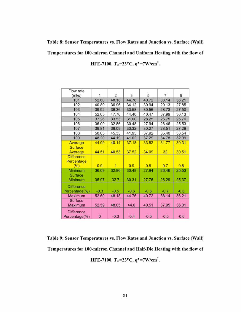
81
Table 8: Sensor Temperatures vs. Flow Rates and Junction vs. Surface (Wall)
Temperatures for 100-micron Channel and Uniform Heating with the flow of
HFE-7100, Tin=23°C, q!=7W/cm2.
Flow rate
(ml/s) 1 2 3 5 7 9
101 52.60 48.18 44.76 40.72 38.14 36.21
102 40.89 36.96 34.12 30.94 29.13 27.85
103 39.92 36.36 33.58 30.56 28.73 27.50
104 52.05 47.76 44.40 40.47 37.99 36.13
105 37.26 33.53 31.00 28.25 26.75 25.76
106 36.09 32.86 30.48 27.94 26.46 25.53
107 39.81 36.09 33.32 30.27 28.51 27.29
108 50.05 45.33 41.95 37.92 35.40 33.54
109 48.20 44.19 41.02 37.29 34.78 32.99
Average 44.09 40.14 37.18 33.82 31.77 30.31
Surface Average 44.51 40.53 37.52 34.09 32 30.51
Difference Percentage
(%) 0.9 1 0.9 0.8 0.7 0.6
Minimum 36.09 32.86 30.48 27.94 26.46 25.53
Surface Minimum 35.97 32.7 30.31 27.76 26.29 25.37
Difference Percentage(%) -0.3 -0.5 -0.6 -0.6 -0.7 -0.6
Maximum 52.60 48.18 44.76 40.72 38.14 36.21
Surface Maximum 52.59 48.05 44.6 40.51 37.95 36.01
Difference Percentage(%) 0 -0.3 -0.4 -0.5 -0.5 -0.6
Table 9: Sensor Temperatures vs. Flow Rates and Junction vs. Surface (Wall)
Temperatures for 100-micron Channel and Half-Die Heating with the flow of
HFE-7100, Tin=23°C, q!=7W/cm2.
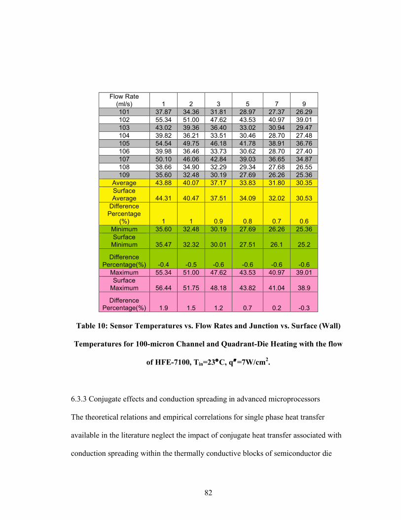
82
Flow Rate (ml/s) 1 2 3 5 7 9
101 37.87 34.36 31.81 28.97 27.37 26.29
102 55.34 51.00 47.62 43.53 40.97 39.01
103 43.02 39.36 36.40 33.02 30.94 29.47
104 39.82 36.21 33.51 30.46 28.70 27.48
105 54.54 49.75 46.18 41.78 38.91 36.76
106 39.98 36.46 33.73 30.62 28.70 27.40
107 50.10 46.06 42.84 39.03 36.65 34.87
108 38.66 34.90 32.29 29.34 27.68 26.55
109 35.60 32.48 30.19 27.69 26.26 25.36
Average 43.88 40.07 37.17 33.83 31.80 30.35
Surface Average 44.31 40.47 37.51 34.09 32.02 30.53
Difference Percentage
(%) 1 1 0.9 0.8 0.7 0.6
Minimum 35.60 32.48 30.19 27.69 26.26 25.36
Surface Minimum 35.47 32.32 30.01 27.51 26.1 25.2
Difference Percentage(%) -0.4 -0.5 -0.6 -0.6 -0.6 -0.6
Maximum 55.34 51.00 47.62 43.53 40.97 39.01
Surface Maximum 56.44 51.75 48.18 43.82 41.04 38.9
Difference Percentage(%) 1.9 1.5 1.2 0.7 0.2 -0.3
Table 10: Sensor Temperatures vs. Flow Rates and Junction vs. Surface (Wall)
Temperatures for 100-micron Channel and Quadrant-Die Heating with the flow
of HFE-7100, Tin=23°C, q!=7W/cm2.
6.3.3 Conjugate effects and conduction spreading in advanced microprocessors
The theoretical relations and empirical correlations for single phase heat transfer
available in the literature neglect the impact of conjugate heat transfer associated with
conduction spreading within the thermally conductive blocks of semiconductor die

83
chips. These theoretical formulations are based on uniform heat flux or uniform
temperature boundary conditions on the surface interacting with the cooling fluid.
Similarly, researchers in the field, when conducting single-phase heat transfer
experiments, strive to produce either a fixed flux or fixed temperature wetted surface.
Thus, nearly all the available formulations for predicting the convective heat transfer
coefficient are based on these ideal boundary conditions. Due to the generally non-
uniform heating in an operating chip, and despite the high thermal conductivity of
silicon, conjugate effects must be included in any effort to achieve a precise
temperature prediction for a convectively cooled chip. Consequently, in the current
study, a detailed thermofluid numerical model of the test apparatus and the heated chip
was created and validated by a comparison of the predicted temperatures at the
locations of nine distinct sensors embedded in the “junction” plane of the chip.
The importance of resolving the spatial distribution of heat flux (the heat flux map) at
the wall surface and resultant distribution of the surface heat transfer coefficients for
the 800-micron thick chip with an average conductivity of 120 W/mK, can not be
overstated. Figures 40, 41 and 42 below, graphically illustrate this conduction
spreading effect on the three heating patterns studied, i.e., uniform heating, half die
heating and quadrant die heating, respectively.
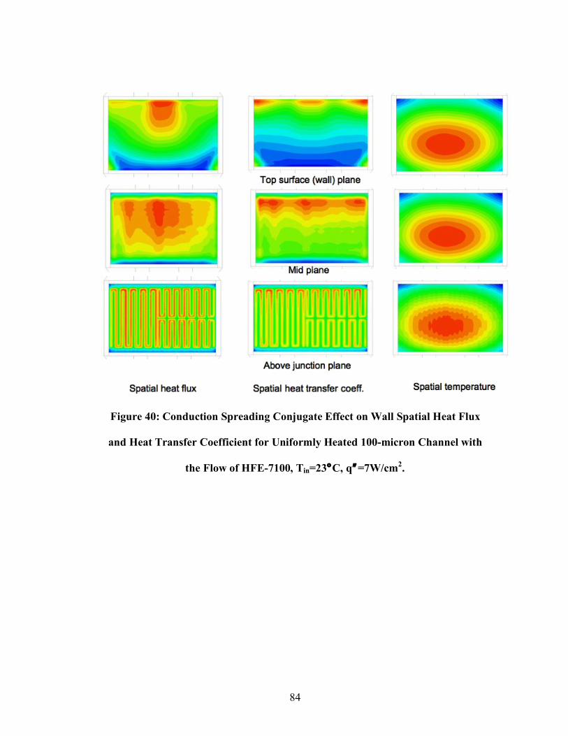
84
Figure 40: Conduction Spreading Conjugate Effect on Wall Spatial Heat Flux
and Heat Transfer Coefficient for Uniformly Heated 100-micron Channel with
the Flow of HFE-7100, Tin=23°C, q!=7W/cm2.
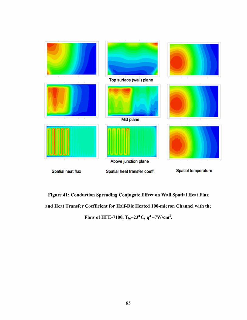
85
Figure 41: Conduction Spreading Conjugate Effect on Wall Spatial Heat Flux
and Heat Transfer Coefficient for Half-Die Heated 100-micron Channel with the
Flow of HFE-7100, Tin=23°C, q!=7W/cm2.
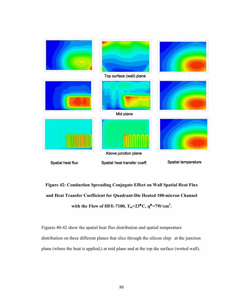
86
Figure 42: Conduction Spreading Conjugate Effect on Wall Spatial Heat Flux
and Heat Transfer Coefficient for Quadrant-Die Heated 100-micron Channel
with the Flow of HFE-7100, Tin=23°C, q!=7W/cm2.
Figures 40-42 show the spatial heat flux distribution and spatial temperature
distribution on three different planes that slice through the silicon chip: at the junction
plane (where the heat is applied,) at mid plane and at the top die surface (wetted wall).
87
The figures reference the results three different heating patterns of the 100-micron
channel flowing HFE-7100 with Tin=23°C and q!=7W/cm2.
While the spatial temperature plots do not change much in pattern, it is clear that the
heat flux distribution on the wetted surface changes dramatically across the thickness
of the silicon die from the junction (bottom) plane to the top surface.
Most importantly, it is found that while the silicon conduction spreading does smooth
out the serpentine pattern applied to the full junction plane of the chip, it does not yield
a uniform heat flux wetted surface. Rather, the combined conduction-convection
effects on this chip with an average heat flux of 6.5W/cm2 result in highly non-uniform
heat flux at the wetted wall, with a peak heat flux reaching 10W/cm2 at the axial
centerline near the inlet to the microgap channel and steep axial and lateral gradients
that yield a flux of 2.5W/cm2 at the channel outlet along the centerline and 4W/cm
2 at
the lateral edges. This highly non-isoflux condition, combined with the non-isothermal
condition, lead to a complex temperature-flux distribution on the wetted surface and
clearly explains why available uniform heat flux correlations failed to predict
accurately the spatial wall heat transfer coefficient.
As with uniform heating, non-uniform heating represented by the half-die heating and
quadrant-die heating shown in Figures 41 and 42, the conjugate effect (die silicon
block conduction spreading) has a similar effect in changing the resultant surface heat
flux and heat transfer coefficient. However, due to the concentrated heat and thus heat
flux at the junction plane with these non-uniform heating types, the resultant surface

88
heat fluxes have a somewhat similar distribution to those at the junction plane. This is
clearly shown in Figures 41 and 42 where the highest heat flux is seen at the same
locations as in the junction plane, i.e., left half of the die with half-die heating and
bottom left quarter of the die with quadrant-die heating.
The availability of the full CFD model makes it possible to refine the calculation of the
heat lost from the junction plane to the larger package and housing of the test chamber.
Consequently, for the evaluation of the efficacy of the apparatus and for determination
of the average heat transfer coefficient, a conjugate thermal analysis was performed to
determine the percentage of heat going into the channel fluid, i.e., the heat conversion
rate versus the heat conducted into the chip substrate and the surrounding structure.
The conversion rate was used in the calculations of the average heat transfer
coefficients shown in Figures 36 and 38. The resulting conversion rates are shown in
Figure 43 for the fluid inlet velocity range considered. It is clearly shown, that the
conversion rate, i.e., heat dissipated across the wetted surface and into the flowing
liquid, increases with the fluid inlet velocity, rising from 7.6W to 9.4W of total chip
power (10W) as the fluid inlet velocity increases from 0.7 m/s to 6.5m/s.
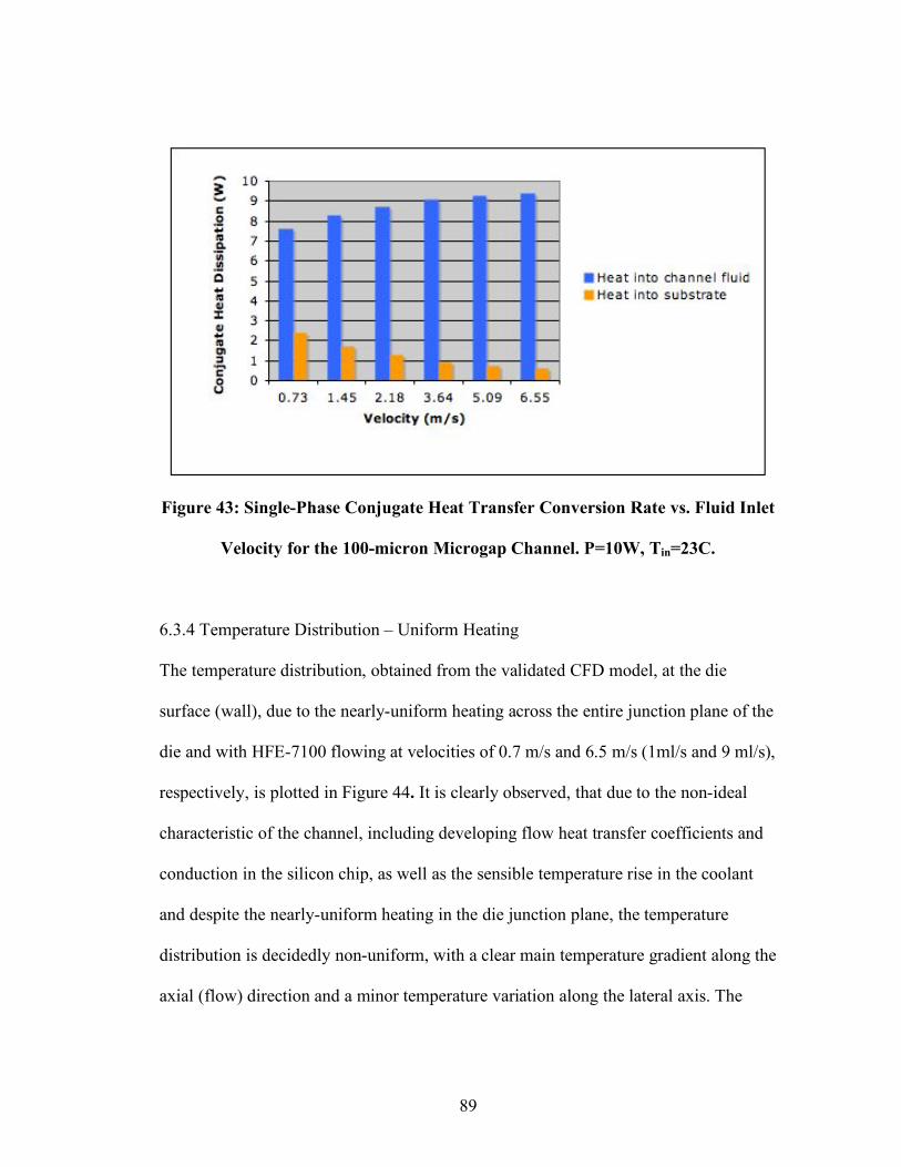
89
Figure 43: Single-Phase Conjugate Heat Transfer Conversion Rate vs. Fluid Inlet
Velocity for the 100-micron Microgap Channel. P=10W, Tin=23C.
6.3.4 Temperature Distribution – Uniform Heating
The temperature distribution, obtained from the validated CFD model, at the die
surface (wall), due to the nearly-uniform heating across the entire junction plane of the
die and with HFE-7100 flowing at velocities of 0.7 m/s and 6.5 m/s (1ml/s and 9 ml/s),
respectively, is plotted in Figure 44. It is clearly observed, that due to the non-ideal
characteristic of the channel, including developing flow heat transfer coefficients and
conduction in the silicon chip, as well as the sensible temperature rise in the coolant
and despite the nearly-uniform heating in the die junction plane, the temperature
distribution is decidedly non-uniform, with a clear main temperature gradient along the
axial (flow) direction and a minor temperature variation along the lateral axis. The
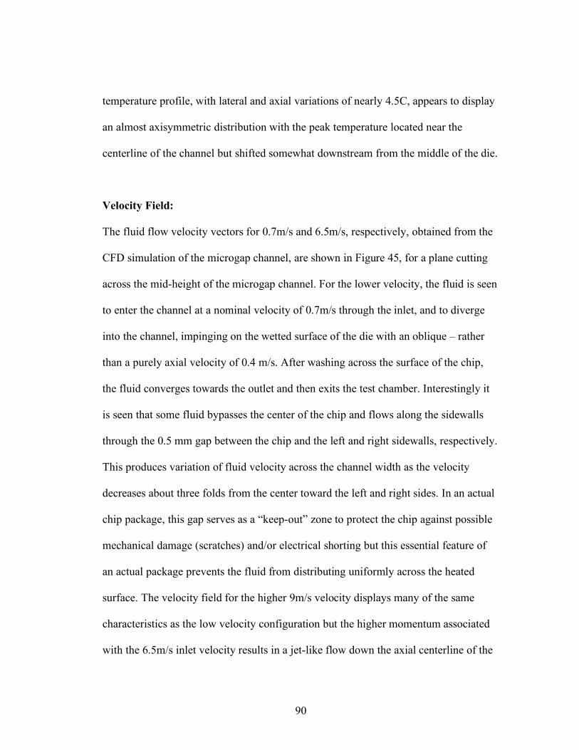
90
temperature profile, with lateral and axial variations of nearly 4.5C, appears to display
an almost axisymmetric distribution with the peak temperature located near the
centerline of the channel but shifted somewhat downstream from the middle of the die.
Velocity Field:
The fluid flow velocity vectors for 0.7m/s and 6.5m/s, respectively, obtained from the
CFD simulation of the microgap channel, are shown in Figure 45, for a plane cutting
across the mid-height of the microgap channel. For the lower velocity, the fluid is seen
to enter the channel at a nominal velocity of 0.7m/s through the inlet, and to diverge
into the channel, impinging on the wetted surface of the die with an oblique – rather
than a purely axial velocity of 0.4 m/s. After washing across the surface of the chip,
the fluid converges towards the outlet and then exits the test chamber. Interestingly it
is seen that some fluid bypasses the center of the chip and flows along the sidewalls
through the 0.5 mm gap between the chip and the left and right sidewalls, respectively.
This produces variation of fluid velocity across the channel width as the velocity
decreases about three folds from the center toward the left and right sides. In an actual
chip package, this gap serves as a “keep-out” zone to protect the chip against possible
mechanical damage (scratches) and/or electrical shorting but this essential feature of
an actual package prevents the fluid from distributing uniformly across the heated
surface. The velocity field for the higher 9m/s velocity displays many of the same
characteristics as the low velocity configuration but the higher momentum associated
with the 6.5m/s inlet velocity results in a jet-like flow down the axial centerline of the
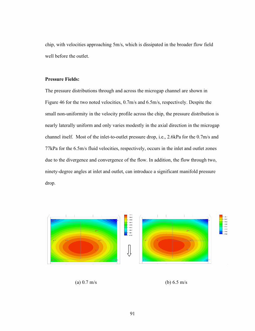
91
chip, with velocities approaching 5m/s, which is dissipated in the broader flow field
well before the outlet.
Pressure Fields:
The pressure distributions through and across the microgap channel are shown in
Figure 46 for the two noted velocities, 0.7m/s and 6.5m/s, respectively. Despite the
small non-uniformity in the velocity profile across the chip, the pressure distribution is
nearly laterally uniform and only varies modestly in the axial direction in the microgap
channel itself. Most of the inlet-to-outlet pressure drop, i.e., 2.6kPa for the 0.7m/s and
77kPa for the 6.5m/s fluid velocities, respectively, occurs in the inlet and outlet zones
due to the divergence and convergence of the flow. In addition, the flow through two,
ninety-degree angles at inlet and outlet, can introduce a significant manifold pressure
drop.
(a) 0.7 m/s (b) 6.5 m/s
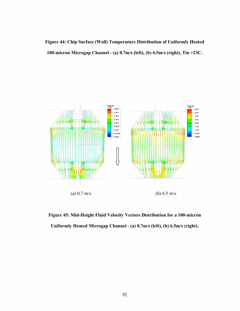
92
Figure 44: Chip Surface (Wall) Temperature Distribution of Uniformly Heated
100-micron Microgap Channel - (a) 0.7m/s (left), (b) 6.5m/s (right), Tin =23C.
(a) 0.7 m/s (b) 6.5 m/s
Figure 45: Mid-Height Fluid Velocity Vectors Distribution for a 100-micron
Uniformly Heated Microgap Channel - (a) 0.7m/s (left), (b) 6.5m/s (right).
93
(a) 0.7 m/s (b) 6.5 m/s
Figure 46: Mid-Height Pressure Distribution for a 100-micron Uniformly Heated
Microgap Channel - (a) 0.7m/s (left), (b) 6.5m/s (right).
6.3.5 Temperature Distribution – Half-Die and Quadrant-Die Heating
The temperature distribution obtained from the simulations performed with the
validated CFD model at the channel wall, due to the non-uniform heating of the die, is
plotted in Figures 47 and 48, for the half-die heating and quadrant-die heating,
respectively, and a fluid inlet temperature of 23°C. It is clearly shown that the
temperature distribution is highly non-uniform. The maximum wall temperature is
located around the middle of the heated half-die and heated quadrant-die for both non-
uniform heating cases, respectively. Larger temperature gradient across the die wall is
seen with the non-uniformity cases compared to the earlier uniformly heated case. A
temperature gradient of 16C is seen with the half-die heated channel and inlet fluid
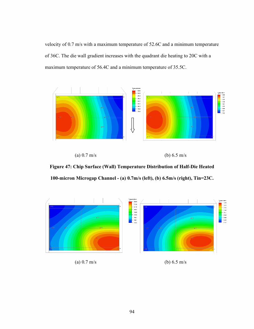
94
velocity of 0.7 m/s with a maximum temperature of 52.6C and a minimum temperature
of 36C. The die wall gradient increases with the quadrant die heating to 20C with a
maximum temperature of 56.4C and a minimum temperature of 35.5C.
(a) 0.7 m/s (b) 6.5 m/s
Figure 47: Chip Surface (Wall) Temperature Distribution of Half-Die Heated
100-micron Microgap Channel - (a) 0.7m/s (left), (b) 6.5m/s (right), Tin=23C.
(a) 0.7 m/s (b) 6.5 m/s

95
Figure 48: Chip Surface (Wall) Temperature Distribution of Quadrant-Die
Heated 100-micron Microgap Channel - (a) 0.7m/s (left), (b) 6.5m/s (right),
Tin=23C.
6.3.6 Inversely Determined Heat Transfer Coefficients
The availability of the detailed thermo-fluid model of the resistance-heated chip
developed in this study also makes it possible to determine the local heat transfer
coefficient, on a cell-by-cell basis, across the die surface based on knowing the cell
temperature and heat flux and the reference temperature, which was assigned to be the
inlet fluid temperature. Applying Newton’s law of cooling on a cell-by-cell basis, the
spatial variations of the heat transfer coefficient across the die surface are shown in
Figure 49 for 0.7m/s and 6.5m/s inlet fluid velocities, respectively. The heat transfer
coefficient distribution for the 0.7m/s inlet fluid velocity, with Re of 380 is nearly
uniform in the lateral direction but varies by a factor of nearly 3.5 in the axial direction,
from a high of 2600 W/m2K at the upstream edge of the chip to 937 W/m
2K at the
downstream edge of the chip. The heat transfer coefficient distribution for the 6.5 m/s
inlet fluid velocity case, with Re of 3420, is highly non-uniform laterally and axially,
varying from a high of 10200 W/m2K at the upstream edge of the chip to 4223 W/m
2K
at the downstream edge of the chip. The higher values of the heat transfer coefficient
and its variation are largely due to the higher fluid velocity associated with the higher
flow rate and the enhanced velocities, previously seen in Fig 41, at the center and sides
of the silicon chip near the liquid inlet to the microgap channel.
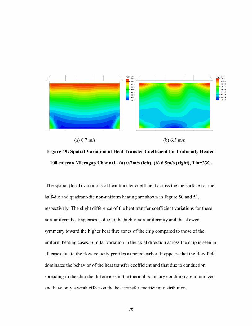
96
(a) 0.7 m/s (b) 6.5 m/s
Figure 49: Spatial Variation of Heat Transfer Coefficient for Uniformly Heated
100-micron Microgap Channel - (a) 0.7m/s (left), (b) 6.5m/s (right), Tin=23C.
The spatial (local) variations of heat transfer coefficient across the die surface for the
half-die and quadrant-die non-uniform heating are shown in Figure 50 and 51,
respectively. The slight difference of the heat transfer coefficient variations for these
non-uniform heating cases is due to the higher non-uniformity and the skewed
symmetry toward the higher heat flux zones of the chip compared to those of the
uniform heating cases. Similar variation in the axial direction across the chip is seen in
all cases due to the flow velocity profiles as noted earlier. It appears that the flow field
dominates the behavior of the heat transfer coefficient and that due to conduction
spreading in the chip the differences in the thermal boundary condition are minimized
and have only a weak effect on the heat transfer coefficient distribution.
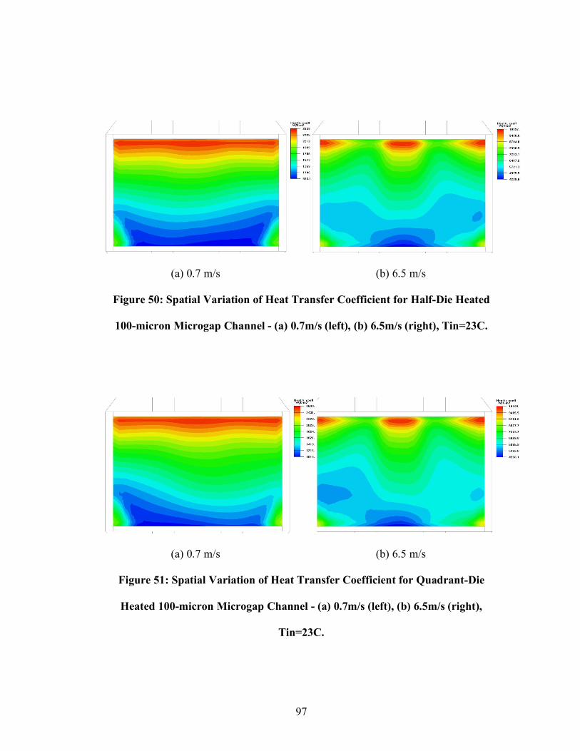
97
(a) 0.7 m/s (b) 6.5 m/s
Figure 50: Spatial Variation of Heat Transfer Coefficient for Half-Die Heated
100-micron Microgap Channel - (a) 0.7m/s (left), (b) 6.5m/s (right), Tin=23C.
(a) 0.7 m/s (b) 6.5 m/s
Figure 51: Spatial Variation of Heat Transfer Coefficient for Quadrant-Die
Heated 100-micron Microgap Channel - (a) 0.7m/s (left), (b) 6.5m/s (right),
Tin=23C.
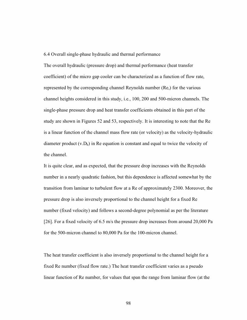
98
6.4 Overall single-phase hydraulic and thermal performance
The overall hydraulic (pressure drop) and thermal performance (heat transfer
coefficient) of the micro gap cooler can be characterized as a function of flow rate,
represented by the corresponding channel Reynolds number (Re,) for the various
channel heights considered in this study, i.e., 100, 200 and 500-micron channels. The
single-phase pressure drop and heat transfer coefficients obtained in this part of the
study are shown in Figures 52 and 53, respectively. It is interesting to note that the Re
is a linear function of the channel mass flow rate (or velocity) as the velocity-hydraulic
diameter product (v.Dh) in Re equation is constant and equal to twice the velocity of
the channel.
It is quite clear, and as expected, that the pressure drop increases with the Reynolds
number in a nearly quadratic fashion, but this dependence is affected somewhat by the
transition from laminar to turbulent flow at a Re of approximately 2300. Moreover, the
pressure drop is also inversely proportional to the channel height for a fixed Re
number (fixed velocity) and follows a second-degree polynomial as per the literature
[26]. For a fixed velocity of 6.5 m/s the pressure drop increases from around 20,000 Pa
for the 500-micron channel to 80,000 Pa for the 100-micron channel.
The heat transfer coefficient is also inversely proportional to the channel height for a
fixed Re number (fixed flow rate.) The heat transfer coefficient varies as a pseudo
linear function of Re number, for values that span the range from laminar flow (at the
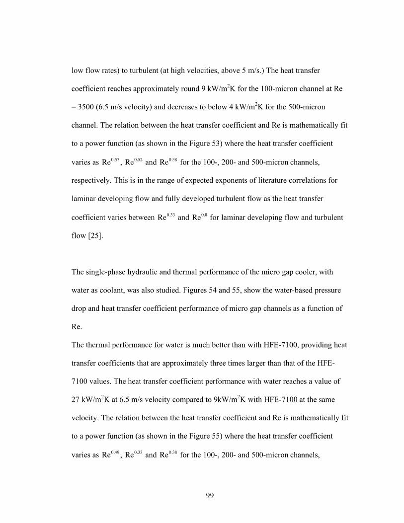
99
low flow rates) to turbulent (at high velocities, above 5 m/s.) The heat transfer
coefficient reaches approximately round 9 kW/m2K for the 100-micron channel at Re
= 3500 (6.5 m/s velocity) and decreases to below 4 kW/m2K for the 500-micron
channel. The relation between the heat transfer coefficient and Re is mathematically fit
to a power function (as shown in the Figure 53) where the heat transfer coefficient
varies as
!
Re0.57 ,
!
Re0.52 and
!
Re0.38 for the 100-, 200- and 500-micron channels,
respectively. This is in the range of expected exponents of literature correlations for
laminar developing flow and fully developed turbulent flow as the heat transfer
coefficient varies between
!
Re0.33 and
!
Re0.8 for laminar developing flow and turbulent
flow [25].
The single-phase hydraulic and thermal performance of the micro gap cooler, with
water as coolant, was also studied. Figures 54 and 55, show the water-based pressure
drop and heat transfer coefficient performance of micro gap channels as a function of
Re.
The thermal performance for water is much better than with HFE-7100, providing heat
transfer coefficients that are approximately three times larger than that of the HFE-
7100 values. The heat transfer coefficient performance with water reaches a value of
27 kW/m2K at 6.5 m/s velocity compared to 9kW/m
2K with HFE-7100 at the same
velocity. The relation between the heat transfer coefficient and Re is mathematically fit
to a power function (as shown in the Figure 55) where the heat transfer coefficient
varies as
!
Re0.49 ,
!
Re0.33 and
!
Re0.38 for the 100-, 200- and 500-micron channels,
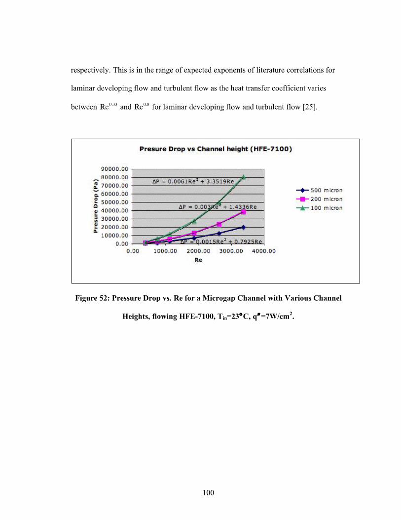
100
respectively. This is in the range of expected exponents of literature correlations for
laminar developing flow and turbulent flow as the heat transfer coefficient varies
between
!
Re0.33 and
!
Re0.8 for laminar developing flow and turbulent flow [25].
Figure 52: Pressure Drop vs. Re for a Microgap Channel with Various Channel
Heights, flowing HFE-7100, Tin=23°C, q!=7W/cm2.
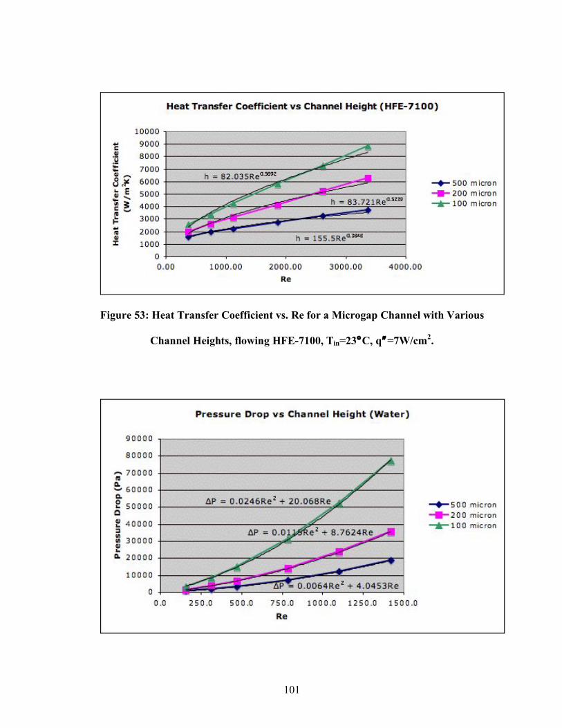
101
Figure 53: Heat Transfer Coefficient vs. Re for a Microgap Channel with Various
Channel Heights, flowing HFE-7100, Tin=23°C, q!=7W/cm2.

102
Figure 54: Pressure Drop vs. Re for a Microgap Channel with Various Channel
Heights, flowing Water, Tin=23°C, q!=7W/cm2.
Figure 55: Heat Transfer Coefficient vs. Re for a Microgap Channel with Various
Channel Heights, flowing Water, Tin=23°C, q!=7W/cm2.
6.5 Conclusions
The chapter discusses in detail the various aspects of single-phase heat transfer for a
chip-scale micro gap channel cooler. Overall pressure drop and heat transfer
coefficient were studied for the various channels considered and with HFE-7100, as
well as water, as the working fluids. The pressure drop was found to be inversely
proportional to the channel height for a fixed Re number (fixed flow rate.) For HFE-
103
7100, the pressure drop, for a fixed velocity of 6.5 m/s, increases from around 20,000
Pa for the 500-micron channel to 80,000 Pa for the 100-micron channel. The heat
transfer coefficient is also inversely proportional to the channel height for a fixed Re
number (fixed velocity.) The heat transfer coefficient function is pseudo linear as a
function of Re number spanning the range from laminar to turbulent at high flow rates
(above 5 m/s.) For HFE-7100, the heat transfer coefficient reaches around 9 kW/m2K
for the 100-micron channel at around Re = 3500 (6.5 m/s velocity.) This heat transfer
coefficient decreases to below 4 kW/m2K for the 500-micron channel.
The single phase pressure drop performance of micro gap channels, with water, is
similar to that of HFE-7100 across all Re. The thermal performance for water,
however, is much better than with HFE-7100. It is around three times larger than that
of HFE-7100. The heat transfer coefficient with water reaches a value of 27 kW/m2K
at 6.5 m/s velocity compared to 9 kW/m2K with HFE-7100 at the same velocity.
The literature correlations for pressure drop and heat transfer coefficient are well
suited for ideal channels with ideal boundary conditions, i.e., channel geometries with
the characteristics of uniform the flow, laminar-developing flow, uniform thermal
boundary conditions (flux or temperature) and neglected conjugate heat transfer effects.
The present work focused on a practical channel (non-ideal) with developing flow,
non-uniform heating, non-ideal geometry, and full conjugate heat transfer effects.
Although single-phase correlations captured the general dependence of the pressure
104
drop and the heat transfer coefficient on the flow rate in this microgap channel, they
have proven not to be accurate, especially at the low flow rate range. For HFE-7100
the average error of using the ideal channel pressure drop correlation is 24% and is
highest at the low velocity range (0.7-1.5 m/s.) Similarly, the average heat transfer
coefficient error is 7% and is highest at similar low velocity range (0.7-1.5 m/s.)
Numerical modeling using computational fluid dynamics software (CFD) was used in
order to overcome the inappropriateness of the available correlations. A CFD model
predicted well the conjugate heat transfer effects (the rate of heat dissipated by the
fluid as convective flow) versus the heat conducted through the chip substrate. It was
found, as predicted, that this conversion rate increases proportionally with the flow
rate and inversely with the channel height. Furthermore, CFD simulations correlated
well with experimental data with an error of 5% and much better than ideal channel-
based literature correlations (20% error) as the CFD model takes into account all the
geometric and boundary condition complexities not considered in the simple
correlations. CFD modeling not only predicted well the overall pressure and the heat
transfer coefficient for the various channels considered (5% error) but also predicted
well the junction plane temperature distribution. Another very important and rather
critical aspect that CFD modeling uncovered was the spatial distribution of heat flux at
the wall (die top surface) and resultant wall spatial the heat transfer coefficient.
Conduction spreading of the die silicon block (800-micron thick) played an important
role in changing the wall heat flux variations for all heating patterns considered
(uniform and non-uniform.) It was found that silicon conduction did obscure the
105
serpentine pattern on the wetted surface but always resulted in highly non-uniform
heat flux at the wall even when the heat was applied across the entire junction plane of
the chip. This provides a clear explanation for why available uniform heat flux
correlations failed to predict accurately the heat transfer coefficient. Knowing the wall
spatial variations of temperature and heat flux, CFD was used to inversely calculate
the spatial variations of wall the heat transfer coefficient. The spatial the heat transfer
coefficient was more non-uniform with non-uniform heating and was characterized by
the skewed symmetry toward the higher heat flux zones of the chip compared to
uniform heating. The flow field dominates the behavior of the heat transfer coefficient
and due to conduction spreading in the chip the differences in the thermal boundary
condition are minimized and have only a weak effect on the heat transfer coefficient
distribution.
106
Chapter 7:
Two-Phase Heat Transfer Experimental Data and Discussion
7.1 Introduction and basic relations
Two-phase heat transfer experiments of the 100, 200 and 500-micron channels, with
HFE-7100 coolant, with three different heating patterns (uniform, half die and
quadrant die heating,) were performed and analyzed under fully saturated conditions.
As noted in Chapter 3, the saturated two-phase experiments were performed on a
silicon thermal test chip resembling a commercially available microprocessor with a
total die surface area of 1.44 cm2. The thermal test chip was mounted in a hermetically
sealed chamber, with a predetermined channel height, i.e., 100-, 200- and 500- micron,
whereby cooling fluid HFE-7100 was pumped into it at a preset flow rate. An in-line
heater was used to heat up the fluid, incoming into the test channel, in order to achieve
the saturated condition immediately at the channel inlet. This saturated liquid
condition was determined by cross comparing the fluid inlet temperature against the
fluid inlet pressure, measured by the installed absolute pressure transducer, at the
channel inlet.
The thermal chip is 13.75 mm wide and 10.47 mm long (along the flow direction.)
This very short length is a key characteristic of this non-ideal channel as it causes the
fluid to be developing in the entire channel. The chip is heated by an embedded
107
serpentine heater at the junction plane of the silicon thermal chip. The embedded
heater enabled for various levels of heat fluxes at the thermal chip and various heating
patterns, i.e., uniform heating, half-die and quadrant-die non-uniform heating. A
detailed and overall description of the microgap channel two-phase apparatus is found
in Chapter 3.
The wall (die top surface) temperatures were captured by nine embedded temperature
diodes (sensors) spread at various locations at the thermal chip junction plane. The
heated (two-phase) fluid exiting the microgap channel is run through an externally
water-cooled flat plate heat exchanger to condense the two-phase mixture. The
condensate fluid is pumped through a centrifugal pump at a pre-determined flow rate
back into the channel through the in-line heater. A flow rate meter is installed at the
outlet of the pump to measure the fluid flow rate.
A set of saturated two-phase experiments were run through the 100, 200 and 500
micron channels, with variable mass flow rates and variable heat fluxes at the thermal
test chip.
The average wall temperature was calculated by averaging out the nine temperature
sensors embedded in the test chip. The heat conversion rate, i.e., the percentage of heat
going into the test channel as opposed to the heat conducted through the chip substrate
into the test board, is extracted from the output of the pseudo two-phase CFD model
based on the validated single-phase CFD model. The model, for each fixed flow rate,
heat flux and channel height, was run iteratively by altering the fluid properties until
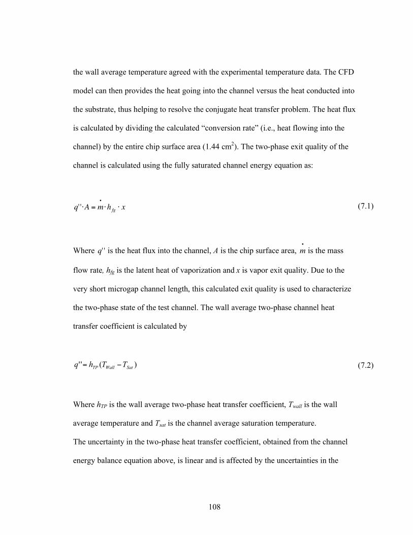
108
the wall average temperature agreed with the experimental temperature data. The CFD
model can then provides the heat going into the channel versus the heat conducted into
the substrate, thus helping to resolve the conjugate heat transfer problem. The heat flux
is calculated by dividing the calculated “conversion rate” (i.e., heat flowing into the
channel) by the entire chip surface area (1.44 cm2). The two-phase exit quality of the
channel is calculated using the fully saturated channel energy equation as:
!
q' '"A = m•
"hfg " x (7.1)
Where
!
q' ' is the heat flux into the channel, A is the chip surface area,
!
m
•
is the mass
flow rate, hfg is the latent heat of vaporization and x is vapor exit quality. Due to the
very short microgap channel length, this calculated exit quality is used to characterize
the two-phase state of the test channel. The wall average two-phase channel heat
transfer coefficient is calculated by
)('' SatWallTP TThq != (7.2)
Where hTP is the wall average two-phase heat transfer coefficient, Twall is the wall
average temperature and Tsat is the channel average saturation temperature.
The uncertainty in the two-phase heat transfer coefficient, obtained from the channel
energy balance equation above, is linear and is affected by the uncertainties in the
109
measured quantities including the flow rate, the temperature of the wall (die sensors),
the temperature at the inlet, and the stability of the data logger and power supply. It
can be expressed mathematically as
!
"h
h
#
$ %
&
' (
2
="m
•
m•
#
$
% %
&
'
( (
2
+"q
q
#
$ %
&
' (
2
+")Twall)Twall
#
$ %
&
' (
2
(7.3)
Where
!
" h is uncertainty of heat transfer coefficient,
!
"m•
is the error of flow rate via
the flow meter,
!
"q is error of input power via the power supply,
!
"#Twall
is the
measurement error of wall super heat temperature. The flow meter’s flow rate error is
± 1.5%. The error of the power supply is ± 2.5%. The maximum error in the wall
super heat temperature measurement is ± 0.25°C which causes maximum error of 1%.
Thus, the possible maximum error of measuring the two-phase heat transfer coefficient
is ±3.1%.
The single-phase heat transfer experimental work detailed in Chapter 5, served to
validate the overall approach of measuring the channel heat transfer coefficient while
identifying the difficulty in applying classical correlations to actual chip cooling with
all the non-idealities we have encountered including flow-based, geometrical,
boundary conditions non-idealities.
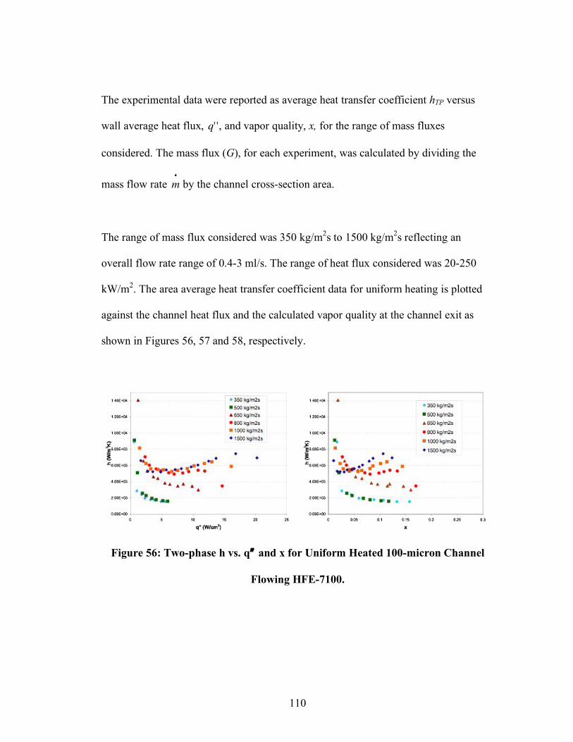
110
The experimental data were reported as average heat transfer coefficient hTP versus
wall average heat flux,
!
q' ', and vapor quality, x, for the range of mass fluxes
considered. The mass flux (G), for each experiment, was calculated by dividing the
mass flow rate
!
m
•
by the channel cross-section area.
The range of mass flux considered was 350 kg/m2s to 1500 kg/m
2s reflecting an
overall flow rate range of 0.4-3 ml/s. The range of heat flux considered was 20-250
kW/m2. The area average heat transfer coefficient data for uniform heating is plotted
against the channel heat flux and the calculated vapor quality at the channel exit as
shown in Figures 56, 57 and 58, respectively.
Figure 56: Two-phase h vs. q! and x for Uniform Heated 100-micron Channel
Flowing HFE-7100.
111
Figure 57: Two-phase h vs. q! and x for Uniform Heated 200-micron Channel
Flowing HFE-7100.
Figure 58: Two-phase h vs. q! and x for Uniform Heated 500-micron Channel
Flowing HFE-7100.
7.2 Taitel-Dukler Flow Regime Map
Following Bar-Cohen and Rahim [20], classical Taitel-Dukler flow regime modeling
was performed on the 100-, 200- and 500-micron uniformly heated channels and the

112
locus of the two-phase mixture, as well as the heat transfer coefficient data, was
superimposed on the TD flow regime maps, as shown in Figures 59-61.
The map’s coordinates are the superficial gas velocity and superficial liquid velocity
given by
!
UG
S= x
G
"G
UL
S= (1# x)
G
"L
(7.4)
Where
!
UG
S is the superficial gas velocity and
!
UL
S is the superficial liquid velocity while
G (kg/m2s) is the mass flux, x is the exit quality and
!
"G
and
!
"L (kg/m
3) are the gas and
liquid density, respectively.
The TD map model determines the flow regime, i.e., Stratified, Bubbly, Intermittent or
Annular, for each binary set of superficial gas velocity and superficial liquid velocity
values.
The channel average heat transfer coefficient data calculated for various heat fluxes
are overlaid on the TD maps as a function of the superficial gas velocity (representing
the exit quality x) for a specific mass flux G.
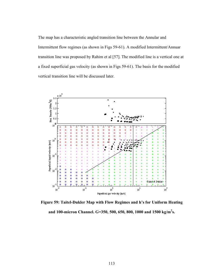
113
The map has a characteristic angled transition line between the Annular and
Intermittent flow regimes (as shown in Figs 59-61). A modified Intermittent/Annuar
transition line was proposed by Rahim et al [57]. The modified line is a vertical one at
a fixed superficial gas velocity (as shown in Figs 59-61). The basis for the modified
vertical transition line will be discussed later.
Figure 59: Taitel-Dukler Map with Flow Regimes and h’s for Uniform Heating
and 100-micron Channel. G=350, 500, 650, 800, 1000 and 1500 kg/m2s.
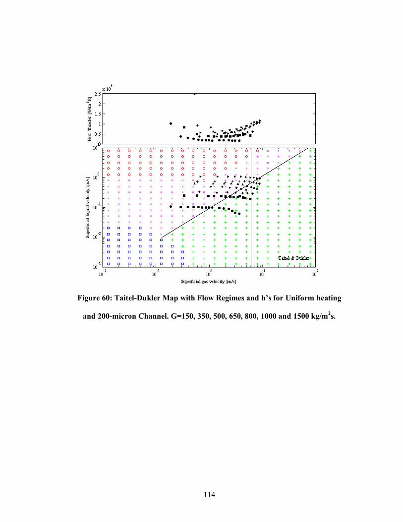
114
Figure 60: Taitel-Dukler Map with Flow Regimes and h’s for Uniform heating
and 200-micron Channel. G=150, 350, 500, 650, 800, 1000 and 1500 kg/m2s.
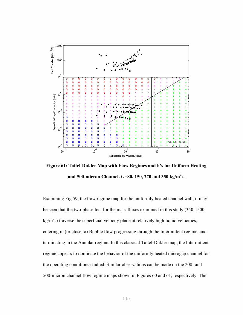
115
Figure 61: Taitel-Dukler Map with Flow Regimes and h’s for Uniform Heating
and 500-micron Channel. G=80, 150, 270 and 350 kg/m2s.
Examining Fig 59, the flow regime map for the uniformly heated channel wall, it may
be seen that the two-phase loci for the mass fluxes examined in this study (350-1500
kg/m2s) traverse the superficial velocity plane at relatively high liquid velocities,
entering in (or close to) Bubble flow progressing through the Intermittent regime, and
terminating in the Annular regime. In this classical Taitel-Dukler map, the Intermittent
regime appears to dominate the behavior of the uniformly heated microgap channel for
the operating conditions studied. Similar observations can be made on the 200- and
500-micron channel flow regime maps shown in Figures 60 and 61, respectively. The
116
two-phase loci for these channels, with the mass fluxes studied (150-1500 kg/m2s for
the 200-micron channel and 80-350 kg/m2s for the 500-micron channel) experience
similar behavior to that of the 100-channel, however at lower overall superficial liquid
velocities such that the loci dos not start with Bubble but rather with Intermittent
regime (especially with the 500-micon channel) terminating at the Annular regime.
Although this mapping methodology has been used successfully for miniature
channels [20] and has helped to establish that Annular flow is the dominant flow
regime for two-phase flow in this form factor, it is to be noted that the present 100-
micron microgap channel, with the exception of the study by Kim et al [19], is
substantially smaller than, and operates at relatively higher mass fluxes, than nearly all
the data examined in the past. While the Tabatabai and Faghri flow regime map [44]
attempts to define a flow regime map for very small diameter tubes, Fig 62 reveals that
this map differs only in the boundary between Bubble and Intermittent flow and does
not alter the location of the Annular flow regime. It has also been suggested that the
Confinement Number, Co, defined as the ratio of the theoretical bubble departure
diameter to the tube diameter, could be used to identify true micro-channels [30]. For
Co > 0.5, individual vapor bubbles could be expected to fill the entire tube, leading to
Intermittent flow, and Co substantially larger than unity, as occurred in the present
work (Co = 4.5 for 100-micron channel and HFE-7100 coolant), would appear to
imply that Annular flow prevails in the channel.
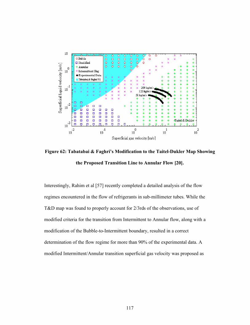
117
Figure 62: Tabatabai & Faghri’s Modification to the Taitel-Dukler Map Showing
the Proposed Transition Line to Annular Flow [20].
Interestingly, Rahim et al [57] recently completed a detailed analysis of the flow
regimes encountered in the flow of refrigerants in sub-millimeter tubes. While the
T&D map was found to properly account for 2/3rds of the observations, use of
modified criteria for the transition from Intermittent to Annular flow, along with a
modification of the Bubble-to-Intermittent boundary, resulted in a correct
determination of the flow regime for more than 90% of the experimental data. A
modified Intermittent/Annular transition superficial gas velocity was proposed as
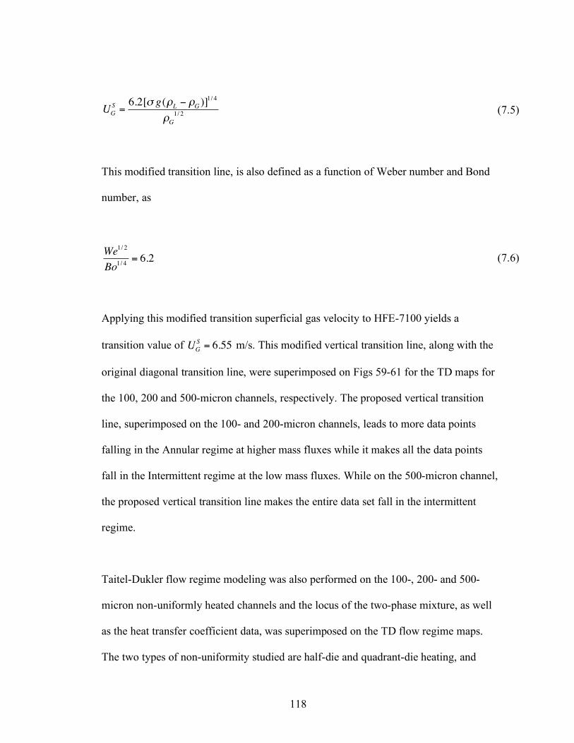
118
!
UG
S=6.2[" g(#L $ #G )]
1/ 4
#G1/ 2
(7.5)
This modified transition line, is also defined as a function of Weber number and Bond
number, as
!
We1/ 2
Bo1/ 4
= 6.2 (7.6)
Applying this modified transition superficial gas velocity to HFE-7100 yields a
transition value of
!
UG
S= 6.55 m/s. This modified vertical transition line, along with the
original diagonal transition line, were superimposed on Figs 59-61 for the TD maps for
the 100, 200 and 500-micron channels, respectively. The proposed vertical transition
line, superimposed on the 100- and 200-micron channels, leads to more data points
falling in the Annular regime at higher mass fluxes while it makes all the data points
fall in the Intermittent regime at the low mass fluxes. While on the 500-micron channel,
the proposed vertical transition line makes the entire data set fall in the intermittent
regime.
Taitel-Dukler flow regime modeling was also performed on the 100-, 200- and 500-
micron non-uniformly heated channels and the locus of the two-phase mixture, as well
as the heat transfer coefficient data, was superimposed on the TD flow regime maps.
The two types of non-uniformity studied are half-die and quadrant-die heating, and
119
their TD flow regime maps as shown in Figures 63-65 and Figures 66-68, for the two
heating types, respectively.
Examining the TD maps for the non-uniformly-heated channels in Figs 63-65, shows
that the two-phase loci for the mass fluxes examined in this study experience similar
trends to the uniformly heated channel, as they traverse the superficial velocity plane
at relatively high liquid velocities, entering in Bubble or Intermittent flow, depending
on the channel diameter, progressing through the Intermittent regime, and terminating
in the Annular regime, with the exception of higher mass fluxes (1000-1500 kg/m2s) as
they terminate at the Intermittent (or at boundary of Intermittent-Annular) regime.
Intermittent regime appears to dominate the behavior of the non-uniformly heated
channel (similarly to the uniformly-heated channel) for the operating conditions
studied.
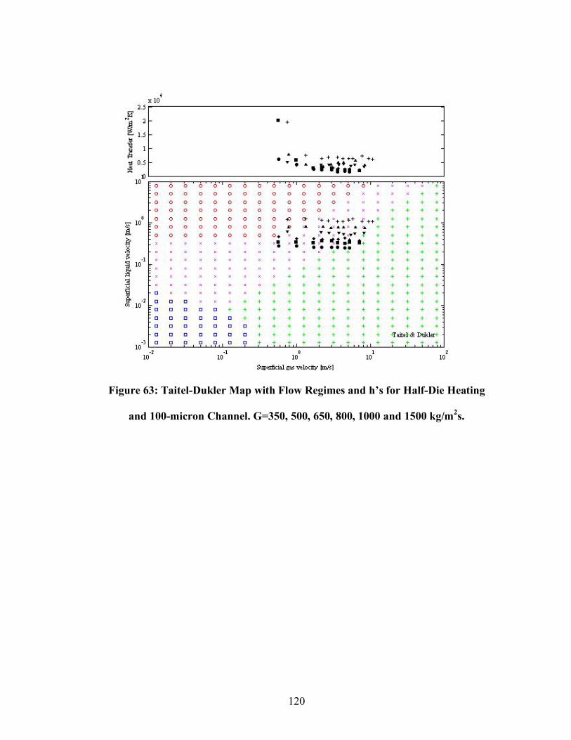
120
Figure 63: Taitel-Dukler Map with Flow Regimes and h’s for Half-Die Heating
and 100-micron Channel. G=350, 500, 650, 800, 1000 and 1500 kg/m2s.
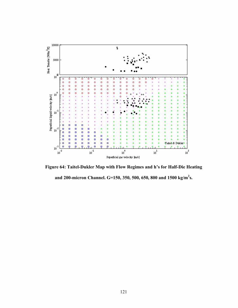
121
Figure 64: Taitel-Dukler Map with Flow Regimes and h’s for Half-Die Heating
and 200-micron Channel. G=150, 350, 500, 650, 800 and 1500 kg/m2s.
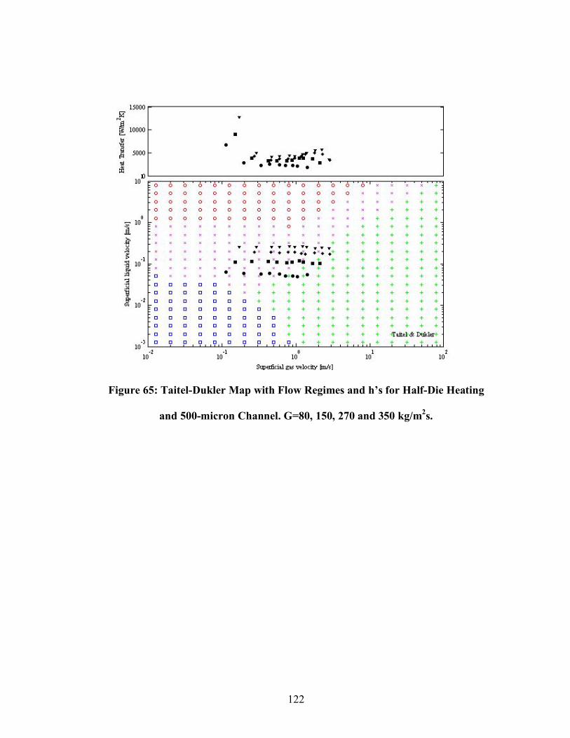
122
Figure 65: Taitel-Dukler Map with Flow Regimes and h’s for Half-Die Heating
and 500-micron Channel. G=80, 150, 270 and 350 kg/m2s.
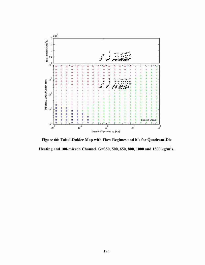
123
Figure 66: Taitel-Dukler Map with Flow Regimes and h’s for Quadrant-Die
Heating and 100-micron Channel. G=350, 500, 650, 800, 1000 and 1500 kg/m2s.

124
Figure 67: Taitel-Dukler Map with Flow Regimes and h’s for Quadrant-Die
Heating and 200-micron Channel. G=150, 350, 500, 650, 800, 1000 and 1500
kg/m2s.
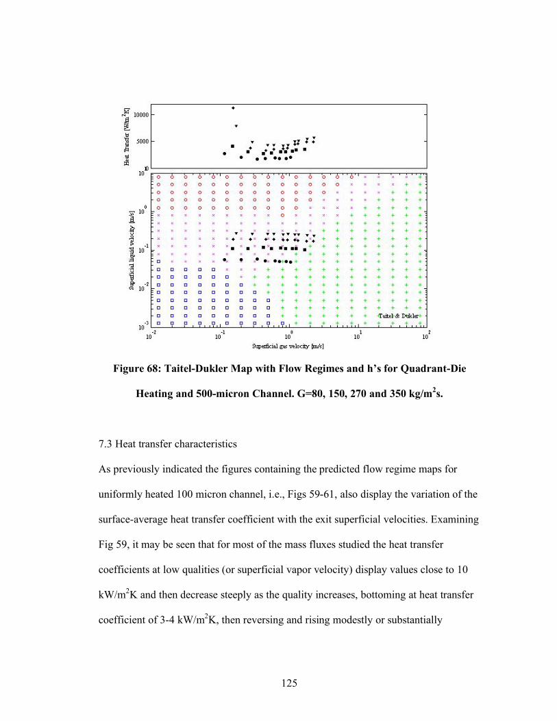
125
Figure 68: Taitel-Dukler Map with Flow Regimes and h’s for Quadrant-Die
Heating and 500-micron Channel. G=80, 150, 270 and 350 kg/m2s.
7.3 Heat transfer characteristics
As previously indicated the figures containing the predicted flow regime maps for
uniformly heated 100 micron channel, i.e., Figs 59-61, also display the variation of the
surface-average heat transfer coefficient with the exit superficial velocities. Examining
Fig 59, it may be seen that for most of the mass fluxes studied the heat transfer
coefficients at low qualities (or superficial vapor velocity) display values close to 10
kW/m2K and then decrease steeply as the quality increases, bottoming at heat transfer
coefficient of 3-4 kW/m2K, then reversing and rising modestly or substantially
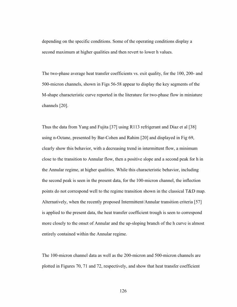
126
depending on the specific conditions. Some of the operating conditions display a
second maximum at higher qualities and then revert to lower h values.
The two-phase average heat transfer coefficients vs. exit quality, for the 100, 200- and
500-micron channels, shown in Figs 56-58 appear to display the key segments of the
M-shape characteristic curve reported in the literature for two-phase flow in miniature
channels [20].
Thus the data from Yang and Fujita [37] using R113 refrigerant and Diaz et al [38]
using n-Octane, presented by Bar-Cohen and Rahim [20] and displayed in Fig 69,
clearly show this behavior, with a decreasing trend in intermittent flow, a minimum
close to the transition to Annular flow, then a positive slope and a second peak for h in
the Annular regime, at higher qualities. While this characteristic behavior, including
the second peak is seen in the present data, for the 100-micron channel, the inflection
points do not correspond well to the regime transition shown in the classical T&D map.
Alternatively, when the recently proposed Intermittent/Annular transition criteria [57]
is applied to the present data, the heat transfer coefficient trough is seen to correspond
more closely to the onset of Annular and the up-sloping branch of the h curve is almost
entirely contained within the Annular regime.
The 100-micron channel data as well as the 200-micron and 500-micron channels are
plotted in Figures 70, 71 and 72, respectively, and show that heat transfer coefficient
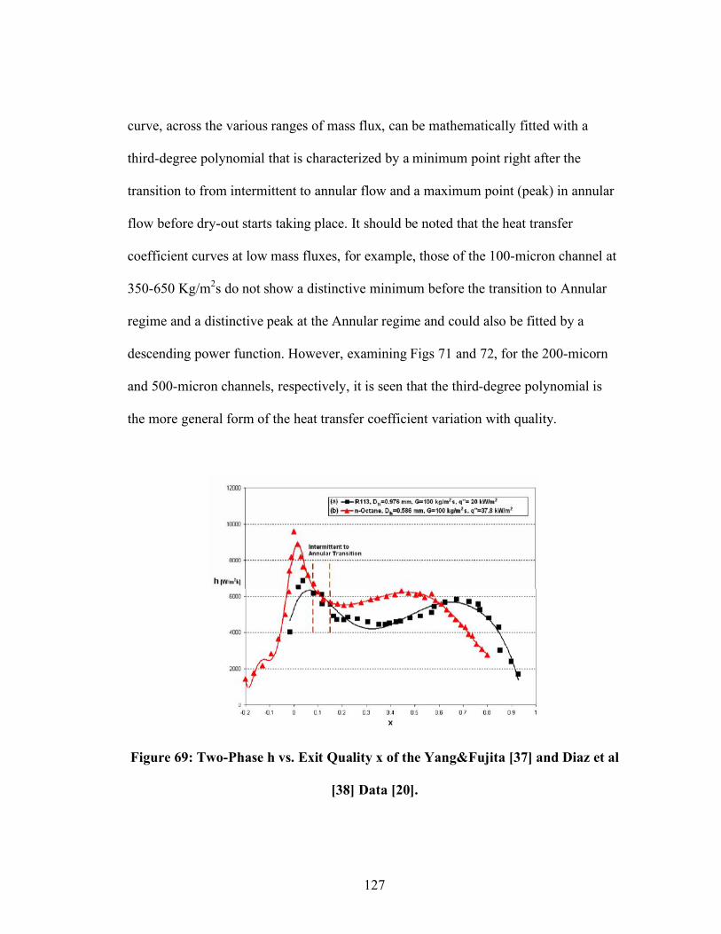
127
curve, across the various ranges of mass flux, can be mathematically fitted with a
third-degree polynomial that is characterized by a minimum point right after the
transition to from intermittent to annular flow and a maximum point (peak) in annular
flow before dry-out starts taking place. It should be noted that the heat transfer
coefficient curves at low mass fluxes, for example, those of the 100-micron channel at
350-650 Kg/m2s do not show a distinctive minimum before the transition to Annular
regime and a distinctive peak at the Annular regime and could also be fitted by a
descending power function. However, examining Figs 71 and 72, for the 200-micorn
and 500-micron channels, respectively, it is seen that the third-degree polynomial is
the more general form of the heat transfer coefficient variation with quality.
Figure 69: Two-Phase h vs. Exit Quality x of the Yang&Fujita [37] and Diaz et al
[38] Data [20].
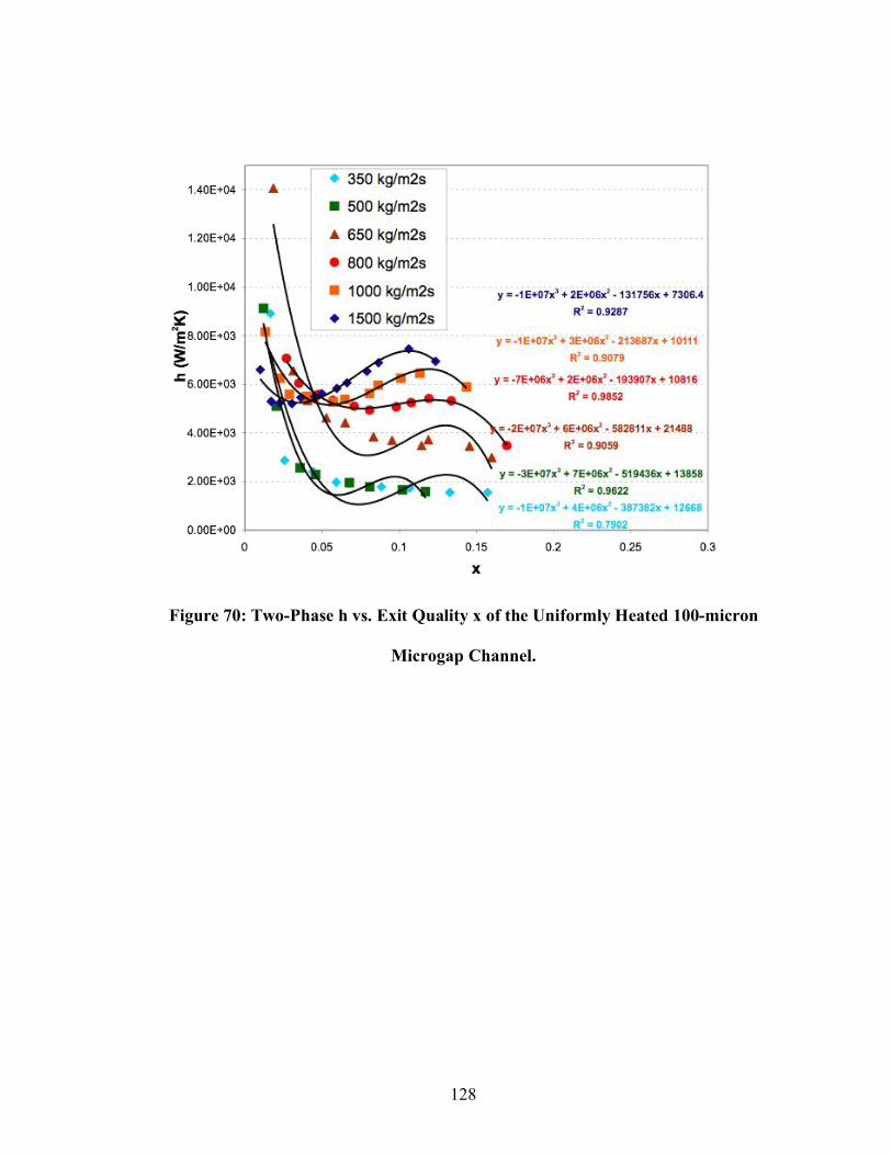
128
Figure 70: Two-Phase h vs. Exit Quality x of the Uniformly Heated 100-micron
Microgap Channel.
129
Figure 71: Two-Phase h vs. Exit Quality x of the Uniformly Heated 200-micron
Microgap Channel.
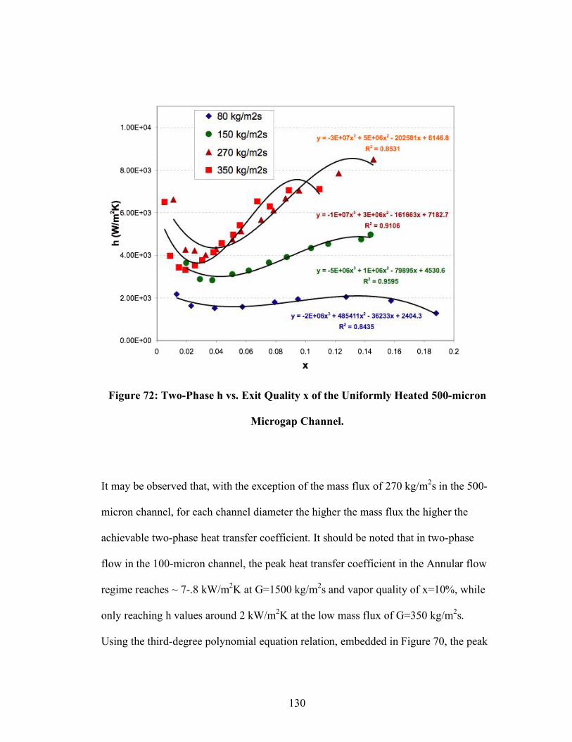
130
Figure 72: Two-Phase h vs. Exit Quality x of the Uniformly Heated 500-micron
Microgap Channel.
It may be observed that, with the exception of the mass flux of 270 kg/m2s in the 500-
micron channel, for each channel diameter the higher the mass flux the higher the
achievable two-phase heat transfer coefficient. It should be noted that in two-phase
flow in the 100-micron channel, the peak heat transfer coefficient in the Annular flow
regime reaches ~ 7-.8 kW/m2K at G=1500 kg/m
2s and vapor quality of x=10%, while
only reaching h values around 2 kW/m2K at the low mass flux of G=350 kg/m
2s.
Using the third-degree polynomial equation relation, embedded in Figure 70, the peak
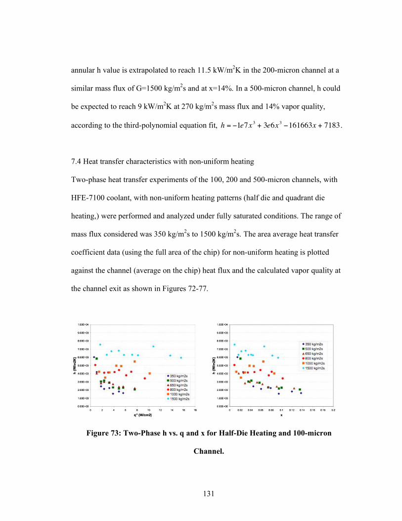
131
annular h value is extrapolated to reach 11.5 kW/m2K in the 200-micron channel at a
similar mass flux of G=1500 kg/m2s and at x=14%. In a 500-micron channel, h could
be expected to reach 9 kW/m2K at 270 kg/m
2s mass flux and 14% vapor quality,
according to the third-polynomial equation fit,
!
h = "1e7x3
+ 3e6x3"161663x + 7183.
7.4 Heat transfer characteristics with non-uniform heating
Two-phase heat transfer experiments of the 100, 200 and 500-micron channels, with
HFE-7100 coolant, with non-uniform heating patterns (half die and quadrant die
heating,) were performed and analyzed under fully saturated conditions. The range of
mass flux considered was 350 kg/m2s to 1500 kg/m
2s. The area average heat transfer
coefficient data (using the full area of the chip) for non-uniform heating is plotted
against the channel (average on the chip) heat flux and the calculated vapor quality at
the channel exit as shown in Figures 72-77.
Figure 73: Two-Phase h vs. q and x for Half-Die Heating and 100-micron
Channel.

132
Figure 74: Two-Phase h vs. q and x for Half-Die Heating and 200-micron
Channel.
Figure 75: Two-Phase h vs. q and x for Half-Die Heating and 500-micron
Channel.
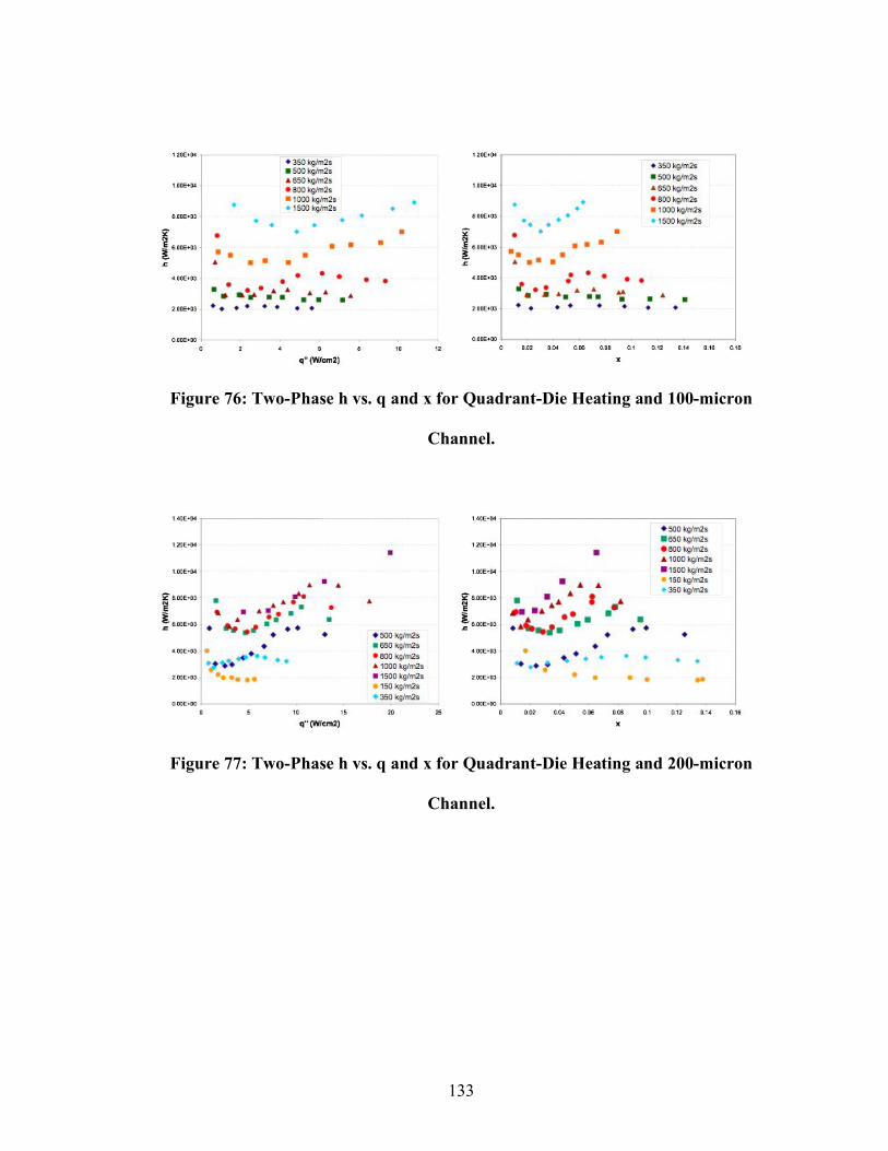
133
Figure 76: Two-Phase h vs. q and x for Quadrant-Die Heating and 100-micron
Channel.
Figure 77: Two-Phase h vs. q and x for Quadrant-Die Heating and 200-micron
Channel.
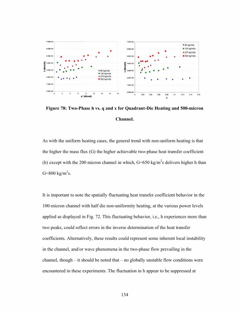
134
Figure 78: Two-Phase h vs. q and x for Quadrant-Die Heating and 500-micron
Channel.
As with the uniform heating cases, the general trend with non-uniform heating is that
the higher the mass flux (G) the higher achievable two-phase heat transfer coefficient
(h) except with the 200 micron channel in which, G=650 kg/m2s delivers higher h than
G=800 kg/m2s.
It is important to note the spatially fluctuating heat transfer coefficient behavior in the
100-micron channel with half die non-uniformity heating, at the various power levels
applied as displayed in Fig. 72. This fluctuating behavior, i.e., h experiences more than
two peaks, could reflect errors in the inverse determination of the heat transfer
coefficients. Alternatively, these results could represent some inherent local instability
in the channel, and/or wave phenomena in the two-phase flow prevailing in the
channel, though – it should be noted that – no globally unstable flow conditions were
encountered in these experiments. The fluctuation in h appear to be suppressed at
135
higher channel heights and higher mass fluxes and can be seen only at low mass flux
levels with the 200 micron channel and completely vanishes with the 500-micron
channel.
Similar h values can be seen with the non-uniform half die heating cases as with the
uniform-heating cases. It should be noted that, with the 100-micron channel h reaches
an annular flow peak of ~7.5 kW/m2K at G=1500 kg/m
2s and vapor quality of x=7%,
while h levels around 2 kW/m2K at the low mass flux of G=350 kg/m
2s. The h value is
extrapolated to increase to around 10 kW/m2K with 200-micron channel at similar
mass flux level of 1500 kg/m2s and at around 8% vapor quality. The two-phase h,
however, goes down to around 2.2 kW/m2K at annular regime peak at G=350 kg/m
2s
and at x=8%. At 500-micron channel, h would reach 6 kW/m2K at 350 kg/m
2s mass
flux and 9% vapor quality level.
Quadrant-die non-uniformity heating shows no h fluctuation observed earlier with
half-die heating. Higher h levels, than those with uniform heating, are observed with
100-micron channel at the high mass flux level of 1500 kg/m2s where the annular flow
regime peak is estimated to be around 10 kW/m2K level and at 8% quality. Similar h
levels, to those with uniform heating, are observed with 200- and 500-micron channels
where h can reach an h value of 13 kW/m2K at 1500 kg/m
2s mass flux with the 200-
micron channel and an extrapolated value of 20 kW/m2K at the same mass flux with
the 500-micron channel.
136
Chapter 8:
Heat Transfer Correlations
8.1 Introduction
Chapter 6 provided a detailed calculation procedure of the two-phase heat transfer
coefficients for the various channel heights studied under the three different heating
patterns considered. The heat transfer coefficients obtained for the 100-, 200- and 500-
micron microgaps were compared to the predictions of the aforementioned Chen and
Shah correlations detailed in Chapter 4. Statistical analysis was performed to
determine the discrepancy between the values predicted by each of the correlations and
the channel heat transfer data. The relative discrepancy in the prediction of heat
transfer coefficients was calculated as:
!
"i =hmeasured
#hcorrelation
hmeasured
$100 (8.1)
And the average relative discrepancy for a set of data was calculated as:
!
"AVE ="i
ni=1
n
# (8.2)
137
A total number of 459 data points (experiments) were performed on all channels (100,
200 and 500-micron) and with three different heating types, i.e., uniform, half-die and
quadrant -die heating.
8.2 Dependence on Two-Phase Reynolds Number
As previously noted in Chapter 3, the dependence of the two-phase heat transfer
coefficient on the two-phase Reynolds Number underpins many of the classical and
commonly used two-phase heat transfer correlations. It is, therefore, of interest to
examine the variation of the two-phase heat transfer coefficient as a function of the
two-phase Reynolds number, defined in equation (3.16). The two-phase data of the
uniformly heated 100-, 200- and 500-micron microgap channels are plotted in Fig 79.
Figure 79 illustrates that the heat transfer coefficient versus two-phase Reynolds
number data are widely scattered, with no clear trend but an apparent tendency for a
stronger dependence at the lower Reynolds Numbers and a weaker dependence at the
higher values. The best fit found for the data is a power function h=68.3Retp0.68
with an
average error of 25.3% (equal to R2=0.67) and a maximum error of 106%.

138
Figure 79: Two-Phase Heat Transfer Coefficient versus Retp for All Uniformly
Heated Microgap Channels.
This less than satisfactory power law dependence on the two-phase Reynolds Number
is thought to reflect the inherent contribution of the distinct flow regimes encountered
in two-phase flow in the microgap channel. It is, thus, appropriate to look at the data
sorted by the different two-phase flow regimes as a way of improving the comparison
and correlation of the heat transfer coefficients. This approach is discussed in detail in
the subsequent sections.
8.3 Flow regime sorting based on TD transition line
The T&D flow regime maps for uniformly heated channels, shown in Chapter 7, are
used to sort the two-phase datasets into Annular and Intermittent flow regimes. Two
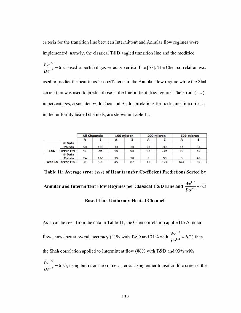
139
criteria for the transition line between Intermittent and Annular flow regimes were
implemented, namely, the classical T&D angled transition line and the modified
!
We1/ 2
Bo1/ 4
= 6.2 based superficial gas velocity vertical line [57]. The Chen correlation was
used to predict the heat transfer coefficients in the Annular flow regime while the Shah
correlation was used to predict those in the Intermittent flow regime. The errors (
!
"AVE ),
in percentages, associated with Chen and Shah correlations for both transition criteria,
in the uniformly heated channels, are shown in Table 11.
Table 11: Average error (
!
"AVE ) of Heat transfer Coefficient Predictions Sorted by
Annular and Intermittent Flow Regimes per Classical T&D Line and
!
We1/ 2
Bo1/ 4
= 6.2
Based Line-Uniformly-Heated Channel.
As it can be seen from the data in Table 11, the Chen correlation applied to Annular
flow shows better overall accuracy (41% with T&D and 31% with
!
We1/ 2
Bo1/ 4
= 6.2) than
the Shah correlation applied to Intermittent flow (86% with T&D and 93% with
!
We1/ 2
Bo1/ 4
= 6.2), using both transition line criteria. Using either transition line criteria, the
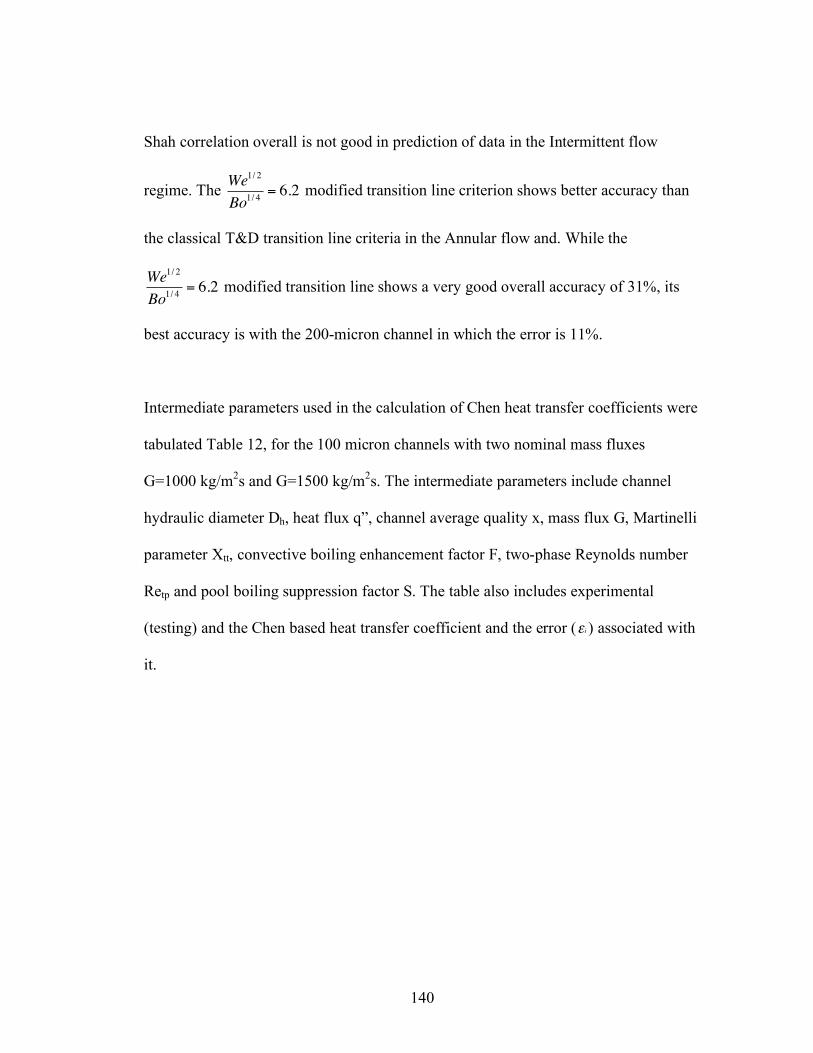
140
Shah correlation overall is not good in prediction of data in the Intermittent flow
regime. The
!
We1/ 2
Bo1/ 4
= 6.2 modified transition line criterion shows better accuracy than
the classical T&D transition line criteria in the Annular flow and. While the
!
We1/ 2
Bo1/ 4
= 6.2 modified transition line shows a very good overall accuracy of 31%, its
best accuracy is with the 200-micron channel in which the error is 11%.
Intermediate parameters used in the calculation of Chen heat transfer coefficients were
tabulated Table 12, for the 100 micron channels with two nominal mass fluxes
G=1000 kg/m2s and G=1500 kg/m
2s. The intermediate parameters include channel
hydraulic diameter Dh, heat flux q”, channel average quality x, mass flux G, Martinelli
parameter Xtt, convective boiling enhancement factor F, two-phase Reynolds number
Retp and pool boiling suppression factor S. The table also includes experimental
(testing) and the Chen based heat transfer coefficient and the error (
!
"i ) associated with
it.
141
Table 12: Parameters of Two-Phase Heat Transfer Chen Correlation on 100-
micron Channel, Showing Error Reduction by Setting Convective Enhancement
Term F=1.
Examining the intermediate parameters used in the calculations of Chen correlations,
listed in Table 12, it is important to note that the value of the nucleate boiling
suppression factor (S) across all cases studied was very close to 1 (this is actually true
for the entire 459 data sets used in the study.) Also, the two-phase Reynolds number
(Retp) experienced very low values across the data set (< 1700). In addition, the
142
average superficial gas velocity of the data points in Fig 59 is ~ 5m/s while the average
superficial liquid velocity is ~ 0.5 m/s. Therefore, for the expected void fractions in the
channel of more than 50%, relatively modest differences between the actual liquid and
vapor velocities might be encountered for the conditions studied in the channel,
suggesting that the convective enhancement in this study could be modest and that
setting F equal to unity may better capture the heat transfer rate in the studied
microgap channel. This was implemented and the values predicted by the Chen
correlation with F=1 were shown in the same table (Table 1) above.
8.4 Pseudo flow regime sorting based on the heat transfer coefficient characteristic
curve
While sorting the data based on the T&D flow regime maps, utilizing the two criteria
mentioned above for transition between Intermittent and Annular flows, did not show
very good overall accuracy, an attempt was made to sort the entire data based on the
characteristic features of the heat transfer coefficient vs. quality curve discussed in
details in Chapter 7. The sorted flow regimes, based on the characteristic h vs. x curve,
will be denoted “Pseudo Intermittent” and “Pseudo Annuar”.
The errors (
!
"AVE ) associated with pseudo Chen and pseudo Shah correlations were
tabulated in Tables 13-18, where Tables 13-14 are for uniform heating, Tables 15-16
are for half-die non-uniform heating while Tables 17-18 are for quadrant-die non-
uniform heating. As can be seen from the error tables, for each heating pattern, the
error data was categorized by channel height, i.e., 100, 200 or 500 micron, and was
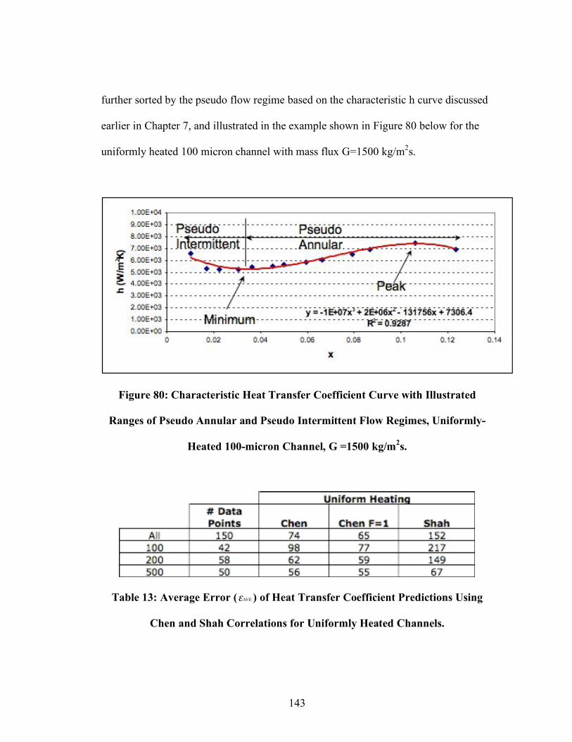
143
further sorted by the pseudo flow regime based on the characteristic h curve discussed
earlier in Chapter 7, and illustrated in the example shown in Figure 80 below for the
uniformly heated 100 micron channel with mass flux G=1500 kg/m2s.
Figure 80: Characteristic Heat Transfer Coefficient Curve with Illustrated
Ranges of Pseudo Annular and Pseudo Intermittent Flow Regimes, Uniformly-
Heated 100-micron Channel, G =1500 kg/m2s.
Table 13: Average Error (
!
"AVE ) of Heat Transfer Coefficient Predictions Using
Chen and Shah Correlations for Uniformly Heated Channels.
144
Table 14: Average Error (
!
"AVE ) of Heat Transfer Coefficient Predictions Sorted by
Pseudo Annular and Pseudo Intermittent Flow regimes Graphically per (h vs. x)
Characteristic Curve, for Uniformly Heated Channels.
Table 15: Average Error (
!
"AVE ) of Heat Transfer Coefficient Predictions Using
Chen and Shah Correlations for Half-Die Heated Channels.

145
Table 16: Average Error (
!
"AVE ) of Heat Transfer Coefficient Predictions Sorted by
Pseudo Annular and Pseudo Intermittent Flow regimes Graphically per (h vs. x)
Characteristic Curve, for Half-Die Heated Channels.
Table 17: Average Error (
!
"AVE ) of Heat Transfer Coefficient Predictions Using
Chen and Shah Correlations for Quadrant Heated Channels.

146
Table 18: Average Error (
!
"AVE ) of Heat Transfer Coefficient Predictions Sorted by
Pseudo Annular and Pseudo Intermittent Flow regimes Graphically per (h vs. x)
Characteristic Curve, for Quadrant Heated Channels.
Looking at the uniform heating category as a reference for comparing the Chen and
Shah correlations, as these correlations were established for uniform heat flux wall
pipes in the first place, it is clear the Chen and Shah correlations predict well data in
the pseudo Annular and pseudo Intermittent flow regimes, respectively. Chen’s overall
average error for predicting pseudo Annular flow regime data is 22% while that of
Shah for predicting pseudo Intermittent flow regime data is 38%. Chen’s best accuracy
is with the 200-micron channel (17%) followed by the 500-micron channel (23%) and
the 100-micron channel (30%). The accuracy of the Shah correlation prediction in the
intermittent regime improves with the increase of channel height, where it is of an
average error of 46% for the 100-micron channel, 35% for the 200-micron channel and
27% for the 500-micron channel.
Categorizing the data for the non-uniform heating patterns and showing the two
different types of non-uniformity considered in the study, along with the sorting by the
slope of the heat transfer coefficient curve, as shown in Tables 13 and 15, shows
similar results to the uniform heating, relative to the accuracy of the Shah predictions.
With the exception of the half-die heating pattern for which the error of the 200-
micron channel (40%) is higher than that of the 100-micron channel (30%) and the
500-micron channel experiences the best accuracy with 22% average error. On the
147
other hand, the Chen correlations show best accuracy with half-die heating (18%) as
compared to that of quadrant-die heating (32%).
The implementation of setting the Chen’s convective boiling enhancement term F
equal to is shown on the correlations accuracy Tables (13-18) for the entire data set.
The biggest effect of setting Chen with F=1 was on the uniformly heated 100 micron
channel, where the error decreases from 30% to 9%. This modification was not helpful
with the higher channels heights.
Looking at the non-uniformly heated channel data in Tables 16 and 18, it can be seen
that similar effect of setting F=1 can be obtained for the 100 micron channel as with
the uniformly heated channel, where the error is reduced from 22% to 14% in the half-
die heated channels and from 21% to 20% in the quadrant-die heated channels. For the
200- and 500-micron channels, this modification of F=1 has also a positive impact on
the overall accuracy error as it dropped by a few percentage points.
8.5 Inverse calculations of spatial heat transfer coefficient
In this section, the previously validated single-phase CFD model is used to inversely
determine the spatial distribution of the two-phase heat transfer coefficient.
Unfortunately, today’s CFD codes are incapable of directly modeling two-phase flow
and it is, thus, not possible to simulate ebullient heat transfer in a microgap channel.
Alternatively, it is possible to iteratively change the channel fluid properties, i.e.,
148
specific heat and thermal conductivity, until the model produces wall temperature
distributions, which closely match the values and the pattern of the experimental
results. The experimental and iteratively simulated temperature data are shown in
Table 19, for the three heating patterns in a 100 micron microgap channel, with 25W
heating and mass flux G=1500 Kg/m2s. The number of trials (using Icepack CFD code
[53]) needed for the iterative process was 4-5 per each case, while the final values for
the adjusted fluid properties, including specific heat and thermal conductivity, were ~
3.2 times higher than those of the single-phase (liquid-only) properties. While it was
very difficult to reach a good agreement, with all the sensor temperature data, on the
wall temperature distributions with the uniformly heated channel case, an attempt was
made to maintain the same wall average temperature as with the experimental results
(shown in Table 19.)
It is interesting to mention that a good agreement, with all the sensor temperature data,
was achieved with the non-uniformly heated channels both in temperature distributions
and wall average temperatures.
The conversion rate, i.e., the percentage of heat going into the channel and the spatial
wall heat flux were determined from the model by solving the conductive resistance on
cell-by-cell basis. Knowing the spatial wall heat flux and temperature distribution as
well as the pre-assigned fluid inlet temperature (saturated temperature from the
experimental cases,) the model was used to calculate and post process the wall heat
transfer coefficient on cell-by-cell basis, i.e., to obtain the spatial distribution of h.
149
This was done by implementing Newton’s second law of cooling on each cell of the
wall.
This spatial wall h, q! and temperature distribution determined by this process are
illustrated in Figures 81, 82 and 83, for the three heating patterns considered, namely,
uniform, half die and quadrant die heating, respectively. These cases represented the
tests with total power of 25W and mass flow rate of 1.6 ml/s (equivalent to G= 1500
Kg/m2s) on the 100-micron channel.
Table 19: Experimental (Two-Phase Test) and Iteratively Adjusted CFD Wall
Temperatures for Three Heating Patterns. 100 micron Channel, 25W, G= 1500
kg/m2s.
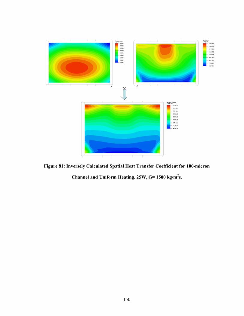
150
Figure 81: Inversely Calculated Spatial Heat Transfer Coefficient for 100-micron
Channel and Uniform Heating. 25W, G= 1500 kg/m2s.
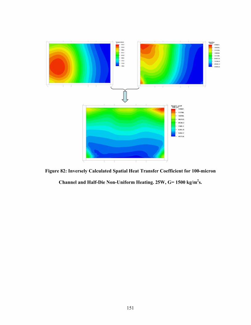
151
Figure 82: Inversely Calculated Spatial Heat Transfer Coefficient for 100-micron
Channel and Half-Die Non-Uniform Heating. 25W, G= 1500 kg/m2s.
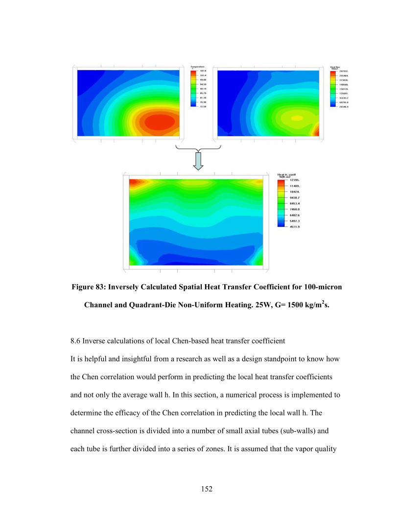
152
Figure 83: Inversely Calculated Spatial Heat Transfer Coefficient for 100-micron
Channel and Quadrant-Die Non-Uniform Heating. 25W, G= 1500 kg/m2s.
8.6 Inverse calculations of local Chen-based heat transfer coefficient
It is helpful and insightful from a research as well as a design standpoint to know how
the Chen correlation would perform in predicting the local heat transfer coefficients
and not only the average wall h. In this section, a numerical process is implemented to
determine the efficacy of the Chen correlation in predicting the local wall h. The
channel cross-section is divided into a number of small axial tubes (sub-walls) and
each tube is further divided into a series of zones. It is assumed that the vapor quality
153
starts at zero at the beginning of all tubes (saturated conditions at channel inlet) and
increases linearly across the tube length to end at the experimentally predetermined
full exit quality at the channel outlet. Having determined the temperature, heat flux and
average quality for each of the zones earlier from CFD, the calculation is performed to
determine the Chen-based h for each of the zones.
These zonal Chen based h calculated values are compared to the zonal CFD based h.
The results are illustrated in Figures 84 and 85, for both uniform heating and non-
uniform heating cases. For the uniform heating case, it can be seen that the spatial
Chen h does not correlate well with the spatial CFD h zonal-wise. While CFD h
decreases axially along the channel axis, we see an opposite pattern, i.e., axial increase
with the Chen h along the channel axis. Chen however correlates well with CFD only
tube-wise if we consider h average values per each of the tubes. This is believed to be
due to the characteristics of geometrical and boundary conditions (non-uniform wall
heat flux) of the channel as being far from ideal channel conditions used in Chen
correlations. For the non-uniform heating case, it quite clear that the spatial Chen h do
not correlate with the spatial CFD h zonal-wise nor do they correlate tube-wise. This is
believed to be due to the same reasons mentioned above especially the highly non-
uniform wall heat flux in both axes of the wall, axially and cross-wise, respectively.
It is believed that the above technique of determination of local Chen based heat
transfer coefficient, can be successful with the implementation of a robust optimization
process for better correlation of local wall temperature distribution between the actual
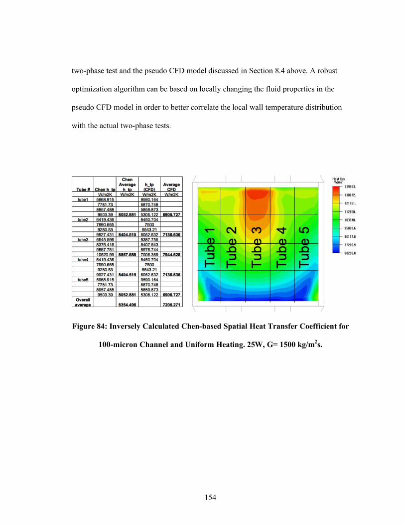
154
two-phase test and the pseudo CFD model discussed in Section 8.4 above. A robust
optimization algorithm can be based on locally changing the fluid properties in the
pseudo CFD model in order to better correlate the local wall temperature distribution
with the actual two-phase tests.
Figure 84: Inversely Calculated Chen-based Spatial Heat Transfer Coefficient for
100-micron Channel and Uniform Heating. 25W, G= 1500 kg/m2s.
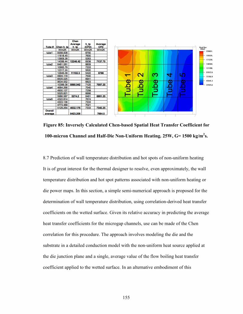
155
Figure 85: Inversely Calculated Chen-based Spatial Heat Transfer Coefficient for
100-micron Channel and Half-Die Non-Uniform Heating. 25W, G= 1500 kg/m2s.
8.7 Prediction of wall temperature distribution and hot spots of non-uniform heating
It is of great interest for the thermal designer to resolve, even approximately, the wall
temperature distribution and hot spot patterns associated with non-uniform heating or
die power maps. In this section, a simple semi-numerical approach is proposed for the
determination of wall temperature distribution, using correlation-derived heat transfer
coefficients on the wetted surface. Given its relative accuracy in predicting the average
heat transfer coefficients for the microgap channels, use can be made of the Chen
correlation for this procedure. The approach involves modeling the die and the
substrate in a detailed conduction model with the non-uniform heat source applied at
the die junction plane and a single, average value of the flow boiling heat transfer
coefficient applied to the wetted surface. In an alternative embodiment of this
156
approach, local values of the heat transfer coefficient could be imposed as the
boundary conditions.
The approach was implemented on the 25W, 1.6 ml/s (1500 kg/m2s) and 100-micron
channel with three different heating patterns, namely, uniform, half die and quadrant
die heating, respectively. Figure 86, shows the wetted wall (top die surface)
temperature distribution, for each of the three cases, of the CFD inversed representing
actual experiment (on the left) versus the CFD with prescribed average CFD inversed
heat transfer coefficient (on the right.) It is clear that this technique predicts well the
wall temperature pattern, including wall average temperature, locations of maximum
temperatures and the temperature rise of the hot spots. The tabulated data of average
and maximum wall temperature for these cases are listed in Table 20. The temperature
differences between the two approaches are very small (1-3°C). The table shows the
error associated with average wall temperatures to be 5.8%, 2.0% and 4.8% for
uniform, half-die and quadrant-de heating patterns, respectively. While the error
associated with maximum wall temperatures to be 5.9%, 5.4% and 2.3% for uniform,
half-die and quadrant-de heating patterns, respectively.
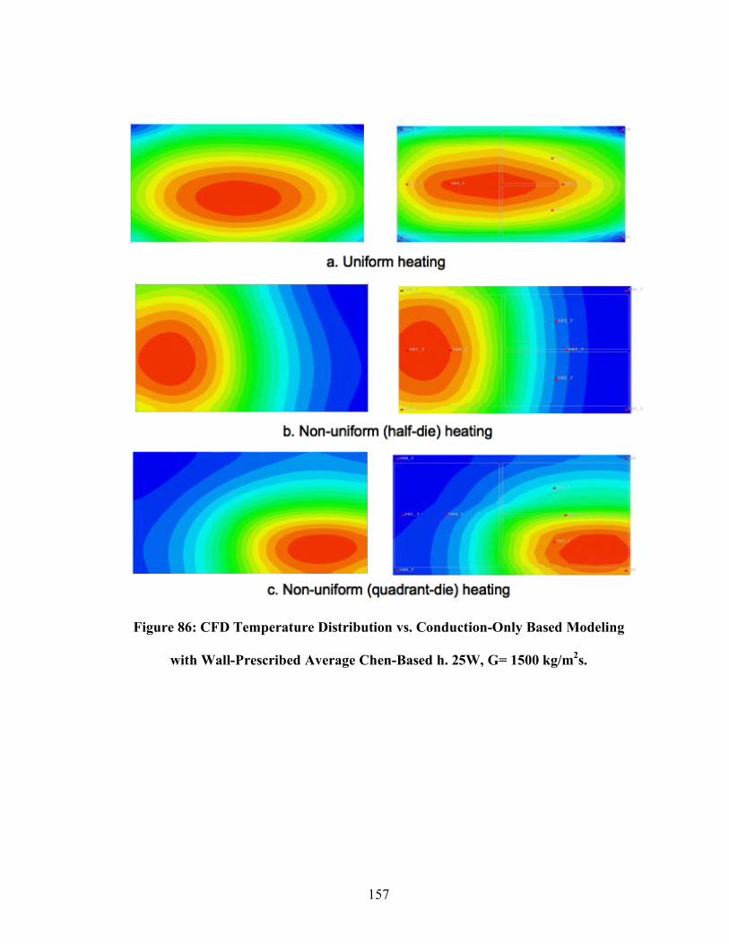
157
Figure 86: CFD Temperature Distribution vs. Conduction-Only Based Modeling
with Wall-Prescribed Average Chen-Based h. 25W, G= 1500 kg/m2s.
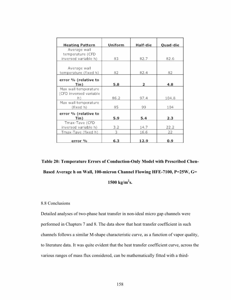
158
Table 20: Temperature Errors of Conduction-Only Model with Prescribed Chen-
Based Average h on Wall, 100-micron Channel Flowing HFE-7100, P=25W, G=
1500 kg/m2s.
8.8 Conclusions
Detailed analyses of two-phase heat transfer in non-ideal micro gap channels were
performed in Chapters 7 and 8. The data show that heat transfer coefficient in such
channels follows a similar M-shape characteristic curve, as a function of vapor quality,
to literature data. It was quite evident that the heat transfer coefficient curve, across the
various ranges of mass flux considered, can be mathematically fitted with a third-
159
degree polynomial that is characterized by a minimum point right after the transition
from intermittent to annular flow and a maximum point (peak) at annular flow.
The general trend of heat transfer coefficient is that the higher the mass flux (G) the
higher achievable two-phase heat transfer coefficient (h) with few exceptions.
Heat transfer coefficient, with the 100-micron channel h reaches an annular flow peak
of ~7.8 kW/m2K at G=1500 kg/m
2s and vapor quality of x=10%. The h value is
extrapolated to increase to around 12 kW/m2K with 200-micron channel at similar
mass flux level of 1500 kg/m2s and at around 15% vapor quality. At 500-micron
channel, h could be expected to reach 9 kW/m2K at 270 kg/m
2s mass flux and 14%
vapor quality level.
The peak two-phase HFE-7100 heat transfer coefficient values were nearly 3-4 times
as high as the single phase HFE-7100 values and sometimes exceed the cooling
capability associated with water under forced convection.
It is important to note the fluctuating behavior, with the 100-micron channel with half
die non-uniformity heating, of the heat transfer coefficient at the various power levels
applied. This fluctuating behavior, i.e., h experiences more than two peaks, could
reflect errors in the inverse determination of the heat transfer coefficients.
Alternatively, these results could represent some inherent local instability in the
channel, and/or wave phenomena in the two-phase flow prevailing in the channel,
though – it should be noted that – no globally unstable flow conditions were

160
encountered in these experiments. The fluctuation in h appear to be suppressed at
higher channel heights and higher mass fluxes and can be seen only at low mass flux
levels with the 200 micron channel and completely vanishes with the 500-micron
channel. Similar thermal performance levels were reported for the non-uniform heating
cases as with the uniform heating ones however at slightly smaller vapor quality levels.
The Taitel-Dukler analytical flow regime map modeling suggests that majority of the
present data falls within the intermittent flow regime. However, it is believed that the
majority of data in this work fall into the annular flow regime. This belief is based on
modifications, by researchers to the T&D flow regime map and its transition line to
annular regime. The belief is also based on the very characteristic trend of heat
transfer coefficient going through the annular regime in the majority of the cases
considered.
While sorting the data based on the T&D flow regime maps, utilizing the original
T&D criterion and the modified
!
We1/ 2
Bo1/ 4
= 6.2 based superficial gas velocity criterion,
for transition between Intermittent and Annular flows, did not show very good overall
accuracy, an attempt was made to sort the entire data graphically based on the
characteristic features of the heat transfer coefficient curve. The sorted flow regimes,
based on the characteristic h vs. x curve, were denoted “Pseudo Intermittent” and
“Pseudo Annuar”.
161
Heat transfer coefficients correlated well with Shah correlations in the pseudo
intermittent flow regime and well with Chen correlations in the pseudo annular flow
regime. Chen’s overall average error for predicting the pseudo annular flow regime
data is 22% while that of Shah for predicting the pseudo intermittent flow regime data
is 38%. Chen’s best accuracy is with the 200-micron channel (17%) followed by the
500-micron channel (23%) and the 100-micron channel (30%). The accuracy of Shah
correlation prediction in the pseudo intermittent regime improves with the increase of
channel height, where it is of an average error of 46% for the 100-micron channel,
35% for the 200-micron channel and 27% for the 500-micron channel.
Categorizing the data per heating patterns and showing the two different types of non-
uniformity considered in the study, along with the flow regime sorting showed similar
correlations with the Shah errors with the exception with the half-die heating pattern
whereby the error of the 200-micron channel (40%) is higher than that of the 100-
micron channel (30%) and the 500-micron channel experiences the best accuracy with
22% average error. On the other hand, Chen correlations show best accuracy with half-
die heating (18%) as compared to that of quadrant-die heating (32%).
Examining the intermediate parameters used in the calculations of Chen correlations,
the value of the nucleate boiling suppression factor (S) across all cases studied was
very close to 1. In addition, the two-phase Reynolds number (Retp) experienced very
low values across the data set (< 1700) suggesting that the convective boiling
enhancement in this study could be modest and that setting F equal to unity may better
162
capture the heat transfer rate in the studied microgap channel. This was implemented
and the biggest effect of setting Chen with F=1 was on the uniformly heated 100
micron channel, where the error decreased from 30% to 9%. This modification was not
helpful with the higher channels heights.
Similar effect, by setting F=1, were obtained with the non-uniformly heated 100-
micron channel as with the uniformly heated channel, where the error is reduced from
22% to 14% in the half-die heated channels and from 21% to 20% in the quadrant-die
heated channels. For the 200- and 500-micron channels, this modification of F=1 had
also a positive impact on the overall accuracy error as it dropped by a few percentage
points.
Inverse calculations of the wall spatial heat transfer coefficient were successfully
demonstrated utilizing CFD. The spatial heat transfer coefficient was correlated with
their counterparts based on implementing Chen correlations. Although Chen provided
accurate predictions spatially with measurements for the uniform heating cases, they
however, did not correlate with the spatial measurements zonal-wise nor do they
correlate tube-wise. This is believed to be due to the highly non-uniform wall heat flux
in both axes of the wall, axially and cross-wise, respectively.
It is believed that the above technique of determination of local Chen based heat
transfer coefficient, can be successful with the implementation of a robust optimization
process for better correlation of local wall temperature distribution between the actual
two-phase test and the pseudo CFD model discussed in Section 8.4 above. A robust
163
optimization algorithm can be based on locally changing the fluid properties in the
pseudo CFD model in order to better correlate the local wall temperature distribution
with the actual two-phase tests.
Finally, a semi-numerical technique was introduced for the prediction of temperature
distribution and hot spots for non-uniform heating. The technique was based on
solving a conduction-only model and prescribing a fixed and uniform Chen based heat
transfer coefficient of the wall. The technique predicted well the wall temperature
pattern including locations for maximum and minimum temperatures including
locations and values of hot spots. The prediction error was largely due to the error
associated with Chen correlations predicting the average wall heat transfer coefficient.

164
Chapter 9:
Conclusions and Future Work
9.1 Conclusions
Microgap channel coolers flowing two-phase dielectric fluid have a good potential for
cooling advanced high power electronics for they provide good thermal performance
and eliminate the inherited TIM thermal resistance prevailing with indirect liquid
cooling techniques. They also can be considered as cost effective and reliable
technique compared to expensive microchannel-based coolers. In order, however, to
address the particular applications in the industry for such microgap channel coolers, a
detailed study of the two-phase performance characteristics under non-ideal conditions
including very short channel length, non-uniformly heated channels, conjugate heat
transfer effect and packaging in a chip-scale form factor. The present work focuses on
experimentally investigating and numerically modeling the two-phase as well as
single-phase characteristics of microgap channels under these practical non-ideal
boundary conditions for a “real world” thermal test chip.
Chapter 6 discussed in detail the various aspects of single-phase heat transfer for a
chip-scale micro gap channel cooler. Single-phase heat transfer and hydraulic
characterization is performed to establish the single-phase baseline performance of the
microgap channel and to validate the mesh-intensive CFD numerical model developed
for the test channel.

165
The pressure drop was found to be inversely proportional to the channel height for a
fixed Re number (fixed velocity.) For HFE-7100, the pressure drop, for a fixed
velocity of 6.5 m/s, increases from around 20,000 Pa for the 500-micron channel to
80,000 Pa for the 100-micron channel. The heat transfer coefficient is also inversely
proportional to the channel height for a fixed Re number (fixed velocity.) The heat
transfer coefficient function is pseudo linear as a function of Re number spanning the
range from laminar to transitional at high flow rates (above 5 m/s.). Convective heat
transfer coefficients for HFE-7100 flowing in a 100-micron microgap channel reached
9 kW/m2K at 6.5 m/s fluid velocity.
The thermal performance for water is much better than with HFE-7100. It is around
three times larger than that of HFE-7100. The heat transfer coefficient with water
reaches a value of 27 kW/m2K at 6.5 m/s velocity.
The literature correlations for pressure drop and heat transfer coefficient are well
suited for ideal channels with ideal boundary conditions, i.e., channel geometries with
the characteristics of uniform the flow, laminar-developing flow, uniform thermal
boundary conditions (flux or temperature) and neglected conjugate heat transfer effects.
The present work focused on a practical channel (non-ideal) with developing flow,
non-uniform heating, non-ideal geometry, and full conjugate heat transfer effects.
Although single-phase correlations captured the general dependence of the pressure
drop and the heat transfer coefficient on the flow rate in this microgap channel, they
have proven not to be accurate, especially at the low flow rate range. For HFE-7100
166
the average error of using the ideal channel pressure drop correlation is 24% and is
highest at the low velocity range (0.7-1.5 m/s.) Similarly, the average heat transfer
coefficient error is 7% and is highest at similar low velocity range (0.7-1.5 m/s.)
Numerical modeling using computational fluid dynamics software (CFD) was
extensively used in order to overcome the inappropriateness of the available
correlations. A mesh intensive CFD model was developed. Despite the highly non-
uniform boundary conditions imposed on the microgap channel, CFD model
simulation gave excellent agreement with the experimental data (to within 5%), while
the discrepancy with the predictions of the classical, “ideal” channel correlations in the
literature reached 20%.
Another very important and rather critical aspect that was uncovered by the CFD mode
was the spatial distribution of heat flux at the wall (die top surface) and resultant wall
spatial the heat transfer coefficient. Conduction spreading of the die silicon block
(800-micron thick) played an important role in changing the wall heat flux variations
for all heating patterns considered (uniform and non-uniform.) It was found that silicon
conduction did obscure the serpentine pattern on the wetted surface but always
resulted in highly non-uniform heat flux at the wall even when the heat was applied
across the entire junction plane of the chip. This provides a clear explanation for why
available uniform heat flux correlations failed to predict accurately the heat transfer
coefficient. Knowing the wall spatial variations of temperature and heat flux, CFD was
used successfully to inversely calculate the spatial variations of wall the heat transfer
167
coefficient. The spatial the heat transfer coefficient was more non-uniform with non-
uniform heating and was characterized by the skewed symmetry toward the higher
heat flux zones of the chip compared to uniform heating. The flow field dominates the
behavior of the heat transfer coefficient and due to conduction spreading in the chip
the differences in the thermal boundary condition are minimized and have only a weak
effect on the heat transfer coefficient distribution.
A detailed investigation of two-phase heat transfer in non-ideal micro gap channels,
with developing flow and significant non-uniformities in heat generation, was
performed in Chapters 7 and 8. Significant temperature non-uniformities were
observed with non-uniform heating, where the wall temperature gradient exceeded
30°C with a heat flux gradient of 3-30 W/cm2, for the quadrant-die heating pattern
compared to a 20°C gradient and 7-14 W/cm2 heat flux gradient for the uniform
heating pattern, at 25W heat and 1500 kg/m2s mass flux.
It is important to note the fluctuating behavior, with the 100-micron channel with half
die non-uniformity heating, of the heat transfer coefficient at the various power levels
applied. This fluctuating behavior, i.e., h experiences more than two peaks, could
reflect errors in the inverse determination of the heat transfer coefficients.
Alternatively, these results could represent some inherent local instability in the
channel, and/or wave phenomena in the two-phase flow prevailing in the channel,
though – it should be noted that – no globally unstable flow conditions were
168
encountered in these experiments. The fluctuation in h appear to be suppressed at
higher channel heights and higher mass fluxes and can be seen only at low mass flux
levels with the 200 micron channel and completely vanishes with the 500-micron
channel. Similar thermal performance levels were reported for the non-uniform heating
cases as with the uniform heating ones however at slightly smaller vapor quality levels.
Taitel-Dukler analytical flow regime map modeling was developed and suggested that
majority of the present data falls within the intermittent flow regime. However, it is
believed that the majority of data in this work fall into the annular flow regime. This
belief is based on modifications, by researchers to the T&D flow regime map and its
transition line to annular regime. The belief is also based on the very characteristic
trend of heat transfer coefficient going through the annular regime in the majority of
the cases considered.
While sorting the data based on the T&D flow regime maps, utilizing the original
T&D criterion and the modified
!
We1/ 2
Bo1/ 4
= 6.2 based superficial gas velocity criterion,
for transition between Intermittent and Annular flows, did not show very good overall
accuracy, an attempt was made to sort the entire data graphically by flow regimes and
type of dependence on quality (variable slope of heat transfer coefficient characteristic
curve). The sorted flow regimes, based on the characteristic h vs. x curve, were
denoted “Pseudo Intermittent” and “Pseudo Annular”.

169
Heat transfer coefficients found to agree well with Shah correlations in the pseudo
intermittent flow regime (38%) and well with Chen correlations in the pseudo annular
flow regime (22%). Chen’s best accuracy is with the 200-micron channel (17%)
followed by the 500-micron channel (23%) and the 100-micron channel (30%). The
accuracy of Shah correlation prediction in the pseudo intermittent regime improves
with the increase of channel height, where it is of an average error of 46% for the 100-
micron channel, 35% for the 200-micron channel and 27% for the 500-micron channel.
Heat transfer coefficient, with the 100-micron channel was found to reach an annular
flow peak of ~8 kW/m2K at G=1500 kg/m
2s and vapor quality of x=10%. The heat
transfer coefficient is extrapolated to increase to around 12 kW/m2K with 200-micron
channel at similar mass flux level of 1500 kg/m2s and at around 15% vapor quality. At
500-micron channel, heat transfer coefficient reaches 9 kW/m2K at 270 kg/m
2s mass
flux and 14% vapor quality level.
The peak two-phase HFE-7100 heat transfer coefficient values were nearly 2.5-4 times
as high as the single phase HFE-7100 values and sometimes exceed the cooling
capability associated with water under forced convection.
Categorizing the data per heating patterns and showing the two different types of non-
uniformity considered in the study, along with the flow regime sorting showed similar
correlations with the Shah errors with the exception with the half-die heating pattern
whereby the error of the 200-micron channel (40%) is higher than that of the 100-
micron channel (30%) and the 500-micron channel experiences the best accuracy with

170
22% average error. On the other hand, Chen correlations show best accuracy with half-
die heating (18%) as compared to that of quadrant-die heating (32%).
Examining the intermediate parameters used in the calculations of Chen correlations,
the value of the nucleate boiling suppression factor (S) across all cases studied was
very close to 1. In addition, the two-phase Reynolds number (Retp) experienced very
low values across the data set (< 1700) suggesting that the convective boiling
enhancement in this study could be modest and that setting F equal to unity may better
capture the heat transfer rate in the studied microgap channel. This was implemented
and the biggest effect of setting Chen with F=1 was on the uniformly heated 100
micron channel, where the error decreased from 30% to 9%. This modification was not
helpful with the higher channels heights.
Similar effect, by setting F=1, were obtained with the non-uniformly heated 100-
micron channel as with the uniformly heated channel, where the error is reduced from
22% to 14% in the half-die heated channels and from 21% to 20% in the quadrant-die
heated channels. For the 200- and 500-micron channels, this modification of F=1 had
also a positive impact on the overall accuracy error as it dropped by a few percentage
points.
The use of inverse computation for determining two-phase heat transfer coefficients
was successfully developed and demonstrated. Further efforts are needed to provide
more precise local wall temperature agreement and enhance the technique accuracy. A
171
robust optimization algorithm can be based on locally changing the fluid properties in
the pseudo CFD model in order to better correlate the local wall temperature
distribution with the actual two-phase tests.
A semi-numerical first-order technique, using the Chen correlation, was found to yield
acceptable prediction accuracy (17%) for the wall temperature distribution and hot
spots in non-uniformly heated “real world” microgap channels cooled by two-phase
flow. The technique was based on solving a conduction-only model and prescribing a
fixed and uniform Chen based heat transfer coefficient of the wall. The technique
predicted well the wall temperature pattern including locations for maximum and
minimum temperatures including locations and values of hot spots. The prediction
error was largely due to the error associated with Chen correlations predicting the
average wall heat transfer coefficient.
9.2 Future work
In this dissertation a detailed modeling and characterization study of single-phase and
two-phase heat transfer was conducted on a chip-scale non-uniformly heated microgap
channel cooler. Thermal performance limits were established and comparisons with
literature correlations of heat transfer coefficient and analysis of two-phase flow
regimes were carried out. In order to complete the understanding of the thermofluid
characteristics of such microgap channels, a number of future investigations are
suggested as follows:
172
• The sorting the heat transfer coefficient data based on the T&D flow regime
maps, utilizing the original T&D criterion and the modified
!
We1/ 2
Bo1/ 4
= 6.2 based
superficial gas velocity criterion, for transition between Intermittent and
Annular flows, did not show very good overall accuracy. On the other hand,
the sorted flow regimes, based on the characteristic h vs. x curve, showed good
accuracy using the Shah correlation in the “Pseudo Intermittent” flow regime
and the Chen correlation in the “Pseudo Annular” flow regime. It is thus
suggested a revisit of this subject and an extended work on possibly modifying
the classical T&D transition lines for a predict better prediction of flow
regimes in true microgap channels.
• The non-uniform heating and conjugate heat transfer effects are becoming
critical characteristics of contemporary microprocessors and graphics chips
packages. It is therefore, suggested that a future work on analyzing two-phase
flow in microgap channels considers a wider range non-uniform heating
patterns and different heat transfer conjugate effects.
• It is helpful and insightful from a research as well as a design standpoint to
know how the Chen correlation would perform in predicting the local heat
transfer coefficients and not only the average wall h. The dissertation presented
a numerical process to determine the efficacy of the Chen correlation in
predicting the local wall heat transfer coefficients. It is believed that this
technique can be successful with the implementation of a robust optimization
173
process for better correlation of local wall temperature distribution between the
actual two-phase test and the pseudo CFD model. A suggested future work is
the investigation of a robust optimization algorithm that can be based on
locally changing the fluid properties in the pseudo CFD model in order to
better correlate the local wall temperature distribution with the actual two-
phase tests.
• This dissertation established two-phase heat transfer performance ranges for a
chip-scale microgap channel housing an actual bare die thermal test chip and
flowing HFE-7100. An extension of this study, is suggested, to utilize other
fluids including water/glycol mixtures and lower boiling point Novec fluids
such as HFE-7000 and develop a two-phase thermal performance envelope as a
function of thermo-physical properties of utilized fluids.
174
Bibliography
[1] Murray, C. T., International Electronics Manufacturing Initiative (iNEMI) Thermal
Roadmap, MEPTEC-2005 Symposium, San Jose, 2005.
[2] Mallik, D., Thermal Issues from ITRS Perspective, MEPTEC-2006 Symposium,
San Jose, 2006.
[3] Patel, C., Thermal Management from Chip Core to the Cooling Tower, MEPTEC-
2005 Symposium, San Jose, 2005.
[4] Chrysler, G., Thermal management Challenges for Microprocessors, MEPTEC-
2005 Symposium, San Jose, 2005.
[5] Tosaya, E., Processor Packaging thermal View, MEPTEC-2006 Symposium, San
Jose, 2006.
[6] Goodson, K., Advanced Thermal Management Technologies for Electronic
Systems, MEPTEC-2005 Symposium, San Jose, 2005.
[7] Howes, J., et al., Cooling of an IGBT Drive System with vaporizable Dielectric
Fluid (VDF,) 24th
IEEE Semi-Therm symposium, San Jose, 2008.
[8] Arik, M. and Bar-Cohen, A., “Immersion cooling for high heat flux
microelectronics with dielectric liquids,” 4th
International symposium on advanced
packaging materials, pp. 229-247, March 1998.
[9] You, S., Simon, T. and Bar Cohen, A., “A technique for enhancing boiling heat
transfer with application to cooling of electronic equipment,” I-THERM III, Inter
society conference on thermal phenomena in electronic systems, pp. 65-73, Feb. 1992.
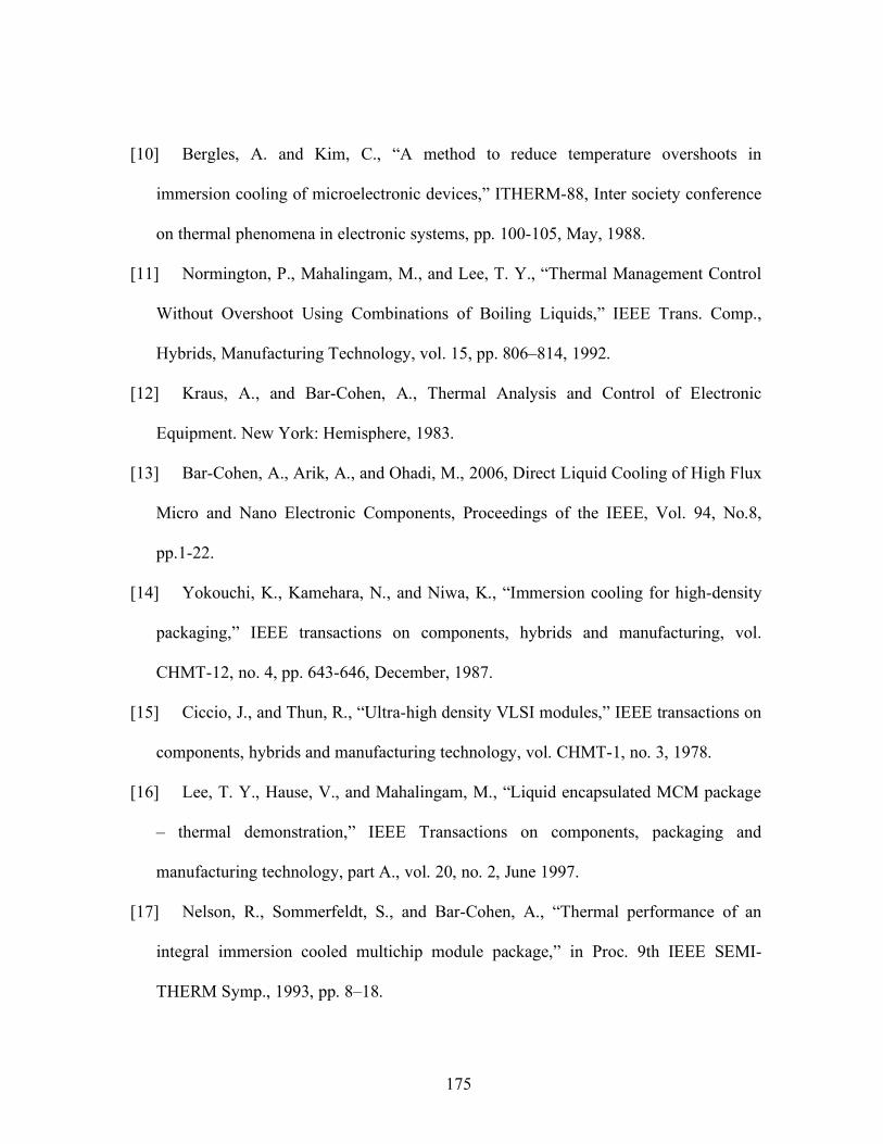
175
[10] Bergles, A. and Kim, C., “A method to reduce temperature overshoots in
immersion cooling of microelectronic devices,” ITHERM-88, Inter society conference
on thermal phenomena in electronic systems, pp. 100-105, May, 1988.
[11] Normington, P., Mahalingam, M., and Lee, T. Y., “Thermal Management Control
Without Overshoot Using Combinations of Boiling Liquids,” IEEE Trans. Comp.,
Hybrids, Manufacturing Technology, vol. 15, pp. 806–814, 1992.
[12] Kraus, A., and Bar-Cohen, A., Thermal Analysis and Control of Electronic
Equipment. New York: Hemisphere, 1983.
[13] Bar-Cohen, A., Arik, A., and Ohadi, M., 2006, Direct Liquid Cooling of High Flux
Micro and Nano Electronic Components, Proceedings of the IEEE, Vol. 94, No.8,
pp.1-22.
[14] Yokouchi, K., Kamehara, N., and Niwa, K., “Immersion cooling for high-density
packaging,” IEEE transactions on components, hybrids and manufacturing, vol.
CHMT-12, no. 4, pp. 643-646, December, 1987.
[15] Ciccio, J., and Thun, R., “Ultra-high density VLSI modules,” IEEE transactions on
components, hybrids and manufacturing technology, vol. CHMT-1, no. 3, 1978.
[16] Lee, T. Y., Hause, V., and Mahalingam, M., “Liquid encapsulated MCM package
– thermal demonstration,” IEEE Transactions on components, packaging and
manufacturing technology, part A., vol. 20, no. 2, June 1997.
[17] Nelson, R., Sommerfeldt, S., and Bar-Cohen, A., “Thermal performance of an
integral immersion cooled multichip module package,” in Proc. 9th IEEE SEMI-
THERM Symp., 1993, pp. 8–18.
176
[18] Geisler, K., Straznicky, I., and Bar-Cohen, A., “Immersion cooling module for
military cots applications,” I-THERM V, Inter society conference on thermal
phenomena in electronic systems, pp. 67-74, June 2004.
[19] Kim, D. W., Rahim, E., Bar-Cohen, A., Han, B., Thermofluid Characteristics of
Two-phase Flow in Micro-Gap Channels, IEEE CPMT, pp. 979-992, 2008.
[20] Bar-Cohen, A. and Rahim, E., Modeling and Prediction of Two-Phase Microgap
Channel Heat Transfer Characteristics, Heat Transfer Engineering, 2008.
[21] Thome, J., Wolverine Engineering Data Book, 2009
[22] Garimella S. V., and Singhal, V., Single-Phase Flow and Heat Transfer and
pumping considerations in microchannel heat sinks, Heat Transfer Engineering, 2004
[23] Kays, W. M. and London, A. L., Compact Heat Exchangers, McGraw-Hill, New
York, 1984.
[24] Shah, R. K. and London, A. L., Laminar Flow Forced Convection in Ducts,
Supplement 1 to Advances in Heat Transfer, Academics, New York, 1978.
[25] Kays, W. M., and Crawford, C., “Convective Heat and Mass Transfer,” McGraw-
Hill, New York, 1966.
[26] Kakac, S., Shah, R., Aung, W., Handbook of Single-Phase Convective Heat
Transfer, John Wiley & Sons, New York, 1978.
[27] Remley, T. J., Abdel-Khalik, S. I., Jeter, S. M., Ghiaasiaan, S. M., and Dowling, M.
F., “Effect of non-uniform heat flux on wall friction and convection heat transfer
coefficient in a trapezoidal channel,” International journal of heat and mass Transfer,
Vol. 44, Issue 13, July 2001.
177
[28] Mehendale, S. S., Jacobi, A. M. and Shah, R. K., Fluid Flow and Heat Transfer at
Micro- and Meso-Scales with Applications to Heat Exchanger Design, Applied Mechanics
Review, Vol. 53, pp. 175-193, 2000.
[29] Kandlikar, S. G. and Grande, W. J., Evolution of Microchannel Flow Passages –
Thermohydraulic Performance and Fabrication Technology, Heat Transfer Engineering,
Vol. 24, no. 1, pp. 3-17, 2003.
[30] Kew, P. A. and Cornwell, K., Correlations for the Prediction of Boiling Heat Transfer
in Small-Diameter Channels, Applied Thermal Engineering, Vol. 17, no. 8-10, pp. 705-
715, 1997.
[31] Liu, Z. and Winterton, R. H. S., A General Correlation for Saturated and Subcooled
Flow Boiling in Tubes and Annuli Based on a Nucleate Boiling Equation, International
Journal of Heat and Mass Transfer, Col. 34, no. 11, pp. 2759-2766, 1991.
[32] Cooper, M. G., Saturated Nucleate Pool Boiling – a Simple Correlation, Proc. of the
1st UK National Heat Transfer Conference, IChemE Symposium, Series Vol. 86 no. 2, pp.
785-793, 1984.
[33] Cooper, M. G., Flow Boiling – the Apparently Nucleate Regime, International Journal
of Heat and Mass Transfer Vol. 32, no. 3, pp. 459-464, 1989.
[34] Lazarek, G. M., Black, S. H., Evaporative Heat Transfer, Pressure Drop, and Critical
Heat Flux in a Small Vertical Tube with R113, International Journal of Heat and Mass
Transfer, Vol. 25, no. 7, pp. 945-960, 1982.
[35] Tran, T. N., Wambsganss, M. W., and France, D. M., Boiling Heat Transfer with
Three Fluids in Small Circular and Rectangular Channels, Argonne National Laboratory
Dept. ANL-95-9. NTIS, Springfield, VA, 1995.
178
[36] Lee, H. J. and Lee, S. Y., Heat Transfer Correlation for Boiling Flows in Small
Rectangular Horizontal Channels with Low Aspect Ratios, International Journal of
Multiphase Flow, Vol. 27, no. 12, pp. 2043-2062, 2001.
[37] Yang, Y., Fujita, Y., Flow Boiling Heat Transfer and Flow Pattern in Rectangular
Channel of Mini-gap, Second International Conference on Microchannels and
Minichannels (ICMM2004-2383), New York, USA, 2004.
[38] Cortina-Diaz, M., and Schmidt, J., Flow Boiling Heat Transfer of n-Hexane and n-
Octane in a Minichannel, Proc. the 13th International Heat Transfer Conference,
Sydney, Australia, 2006.
[39] Madrid, F., Caney, N. and Marty, P., Flow Boiling Study in Mini-Channels,” Proc.
the 4th International Conference on Nanochannels, Microchannels, and Minichannels,
Limerick, Ireland, Paper No. ICNMM2006-96048, 2006.
[40] Taitel, Y., and Dukler, A. E., A Model For Predicting Flow Regime Transitions in
Horizontal and Near Horizontal Gas-Liquid Flow, AIChE Journal, Vol. 22, no. 1, pp.
47-55, 1976.
[41] Taitel, Y., and Dukler, A. E., Effect of Pipe Length on the Transition Boundaries
for High Viscosity Liquids, International Journal of Multiphase Flow, Vol. 13, no. 4,
pp 577-581, 1987.
[42] Bar-Cohen, A., Ruder, Z., and Griffith, P., Thermal and Hydrodynamic Phenomena in
a Horizontal Uniformly Heated Steam Generating Pipe, Journal of Heat Transfer, Vol.
109, no. 3, pp. 739-745, 1987.
179
[43] Weisman, J., Duncan, D., Gibson, J., and Crawford, T., Effect of Fluid Properties and
Pipe Diameter on Two-Phase Flow Pattern in Horizontal Lines, International Journal of
Multiphase Flow, Vol. 5, no. 6, 437-462, 1979.
[44] Tabatabai, A., and Faghri, A., A New Two-Phase Flow Map and Transition Boundary
Accounting for Surface Tension Effects in Horizontal Miniature and Micro Tubes, Journal
of Heat Transfer, v 123, n 5, p 958-968, 2001.
[45] Collier, J. G., and Thome, J. R., “Convective Boiling and Condensation,” Oxford
Science Publications, 2001.
[46] Chen, J. C., Correlation for boiling heat transfer to saturated fluids in convective
flow, Industrial and Engineering Chemistry - Process Design and Development, Vol. 5
no. 3, pp. 322-329, 1966.
[47] Kandlikar, S. G. and Balasubramanian, P., An extension of the flow boiling
correlation to transition, laminar, and deep laminar flows in minichannels and
microchannels, Heat Transfer Engineering, Vol. 25, no. 3, pp. 86-93, 2004.
[48] Gungor, K. E., and Winterton, R. H. S., A General Correlation for Flow Boiling in
Tubes and Annuli, International Journal of Heat and Mass Transfer, Vol. 29, no. 3, pp.
351-358, 1986.
[49] Gungor, K. E., and Winterton, R.H.S., Simplified General Correlation for Saturated
Flow Boiling and Comparisons of Correlations with Data, Chemical Engineering Research
and Design, Vol. 65, no. 2, pp.148-156, 1987.
[50] Shah, M. M., A New Correlation for Heat Transfer During Boiling Flow Through
Pipes, ASHRAE Transactions, Vol. 82, no. 2, pp. 66-86, 1976.
180
[51] Intel “Merom” Processor Test Vehicle, User Guide, November, 2005
[52] 3M Novec Engineering Fluid HFE-7100 for Heat Transfer, 3M, St Paul, MN,
2002.
[53] Icepak CFD Software reference Manual, Ansys, Inc., 2007.
[54] Patankar, S. V., Numerical Heat Transfer and Fluid Flow, Hemisphere, 1980.
[55] Figliola, R. and Beasley, D., Theory and Design for Mechanical Measurements,
John Wiley & Sons, In., 1995.
[56] El-Genk, M. S., Combined Effects of Subcooling and Surface Orientation on Pool
Boiling of HFE-7100 from a Simulated Electronic Chip. Experimental Heat Transfer,
Vol. 16, Issue A, October 2003, pp. 281-301.
[57] Rahim, R., Revellin, R., Thome, J. and Bar-Cohen, A., Characterization and
Prediction of Two-Phase Flow Regimes in Miniature Tubes, Submitted to IJMF,
December 2009.