Characterization of greywater heat

exchangers and the potential of implementation for energy savings

Värmeväxlare för spillvatten –

karakterisering och energibesparingsmöjligheter

JOSE DANIEL GARCIA

MSc-Degree Thesis No.: TRITA-IES 2016:01

Division of Building Service and Energy Systems

Department of Civil and Architectural Engineering

August, 2016

Kungliga Tekniska Högskolan

SE – 100 44 Stockholm

2

ABSTRACT

Buildings account for up to 32% of the total energy use in different countries.

Directives from the European Union have pointed out the importance of increasing

energy efficiency in buildings. New regulation in countries like Sweden establishes

that new buildings should fulfill regulations of Nearly Zero Energy Buildings (NZEB),

opening an opportunity for new technologies to achieve these goals. Almost 80-90%

of the energy in domestic hot water use is wasted from different applications with

almost no use and with a lot of potential energy to be recovered.

The present work studied the characteristics of greywater heat exchanger as a

solution to recuperate heat from greywater to increase efficiency in buildings. This

study explored the fluid mechanics involved in the vertical greywater heat

exchangers, analyzing the falling film effect present in drain pipes and the effects of

the secondary flow generated in the external helical coil. A heat transfer model from

a theoretical approach was proposed and validated. In addition, this study explored

the different variables influencing the economic feasibility of the technology and an

economic analysis was performed. A theoretical comparison between a greywater

heat exchanger application and a reference case without it was evaluated

highlighting the importance of all the variables involved in the potential of

implementation of the technology. The technology shows big potential in households

with high water consumptions, especially with electric boilers.

Keywords: Wastewater heat recovery, greywater heat exchanger, domestic hot

water, energy savings, energy efficiency, residential households, NZEB, heat

transfer modelling, feasibility study, potential of implementation, falling film effect,

flow helical coil.

3

TABLE OF CONTENT

1 INTRODUCTION .............................................................................................. 8

1.1 Heat generation in buildings ....................................................................... 8

1.2 Greywater heat recovery systems (GHRS) ................................................ 9

1.3 Types of Greywater Heat Exchangers...................................................... 10

1.3.1 Vertical heat exchangers ................................................................... 11

1.3.2 Horizontal heat exchangers ............................................................... 11

1.3.3 Shower heat exchangers ................................................................... 11

1.4 Project goals ............................................................................................ 12

1.5 Project boundaries ................................................................................... 12

2 LITERATURE REVIEW .................................................................................. 13

3 FLUID MECHANICS ANALYSIS .................................................................... 15

3.1 Falling film effect ...................................................................................... 15

3.1.1 Falling Film Reynolds ........................................................................ 16

3.1.2 Falling Film Heat Transfer Coefficient ................................................ 17

3.2 Flow through a helical coil ........................................................................ 18

3.2.1 Helical Coil Reynolds Number ........................................................... 18

3.2.2 Dean & Nusselt numbers ................................................................... 20

3.2.3 Heat Transfer coefficient of helical coils ............................................ 22

4 HEAT TRANSFER MODEL ............................................................................ 23

4.1 Inputs of the model ................................................................................... 24

4.2 Thermodynamic properties of the fluid ..................................................... 24

4.3 Thermal Capacities .................................................................................. 26

4.4 Convection Falling Film – R1 ................................................................... 26

4.5 Conduction Drain Pipe – R2 ..................................................................... 26

4.6 Contact Resistance – R3 .......................................................................... 27

4.7 Conduction Coil Pipe – R4 ....................................................................... 28

4.8 Convection Helical Coil – R5 .................................................................... 28

4.9 NTU-Method ............................................................................................. 28

5 MODEL VALIDATION .................................................................................... 30

4

5.1 Nusselt Correlation ................................................................................... 30

5.2 Standard Condition................................................................................... 31

5.3 Different Flow ........................................................................................... 32

5.4 Different dimensions................................................................................. 34

6 MODEL SIMULATIONS ................................................................................. 36

6.1 Dimensions .............................................................................................. 37

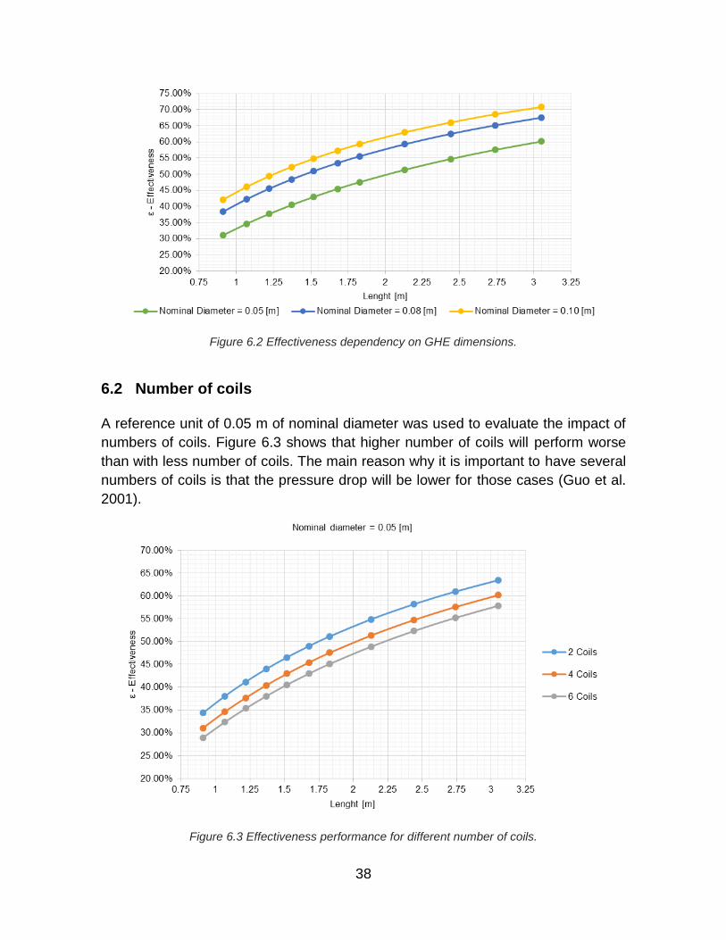
6.2 Number of coils ........................................................................................ 38

6.3 Outlet temperatures.................................................................................. 39

7 POTENTIAL OF IMPLEMENTATION ............................................................ 40

7.1 Water Usage ............................................................................................ 40

7.2 Persons per Household ............................................................................ 43

7.3 Energy price ............................................................................................. 44

7.4 GHRS Unit dimensions & Investment ....................................................... 45

8 ECONOMIC ANALYSIS ................................................................................. 46

8.1 Reference Case ....................................................................................... 46

8.2 GHRS Case ............................................................................................. 47

8.3 Net Present Value .................................................................................... 47

8.4 Discounted Payback Period ..................................................................... 48

8.5 N-number of households – Monte Carlo Simulation ................................. 50

8.6 Emission savings ..................................................................................... 51

8.7 District Heating ......................................................................................... 52

8.8 GHE for multi-dwelling households .......................................................... 54

9 CONCLUSIONS ............................................................................................. 56

10 FUTURE RESEARCH ................................................................................. 58

11 REFERENCES ............................................................................................ 59

APPENDIX A. Heat transfer model ....................................................................... 62

APPENDIX B. Model Validation ............................................................................ 65

APPENDIX C. Model simulations .......................................................................... 68

APPENDIX D. Potential of Implementation ........................................................... 70

APPENDIX E. Screenshots GUI MATLAB ............................................................ 72

5

TABLE OF FIGURES

Figure 1.1 Energy used for heating and hot water in Sweden 2013. ....................... 9

Figure 1.2 Shape of a vertical Greywater Heat Exchanger (GHE). ....................... 10

Figure 3.1 Aspect simulation of a full wetting falling film in a GHRS. .................... 15

Figure 3.2 Falling film formation in vertical oriented GHRS (Left) and fluid

accumulation in horizontal oriented GHRS (right). ................................................ 16

Figure 3.3 Velocity contours [m/s] at different planes along the helical coil. .......... 18

Figure 4.1 Thermal resistors of the heat transfer model. ....................................... 23

Figure 4.2 Top view section with the different geometric diameter of the GHRS (Left)

and Different temperatures inside GHRS (Right). ................................................. 24

Figure 4.3 Heat transfer through contact plane between two solid surfaces. ........ 27

Figure 5.1 Cumulative histogram frequencies of the Heat Recovery Error (Top) and

effectiveness Error (Bottom) for different Nusselt Correlations. ............................. 30

Figure 5.2 Error frequency histogram of the heat transfer model. ......................... 32

Figure 5.3 Average error and standard deviation under different flows. ................ 34

Figure 5.4 Average error of the model under different dimensions. ....................... 34

Figure 6.1 Screenshot from the MATLAB GUI of the model. ................................. 36

Figure 6.2 Effectiveness dependency on GHE dimensions. .................................. 38

Figure 6.3 Effectiveness performance for different number of coils. ...................... 38

Figure 6.4 Simulation for outlet temperatures........................................................ 39

Figure 7.1 Water usage pattern during shower. .................................................... 42

Figure 7.2 Distribution of households in Sweden 2015. ........................................ 43

Figure 7.3. Energy prices for the residential and services sector [öre2013/kWh] ..... 44

Figure 7.4 Electricity price for household consumers 2015 [€/kWh] ...................... 45

Figure 8.1 DPP Analysis for two GHRS under different condition of shower time and

flow. ....................................................................................................................... 49

Figure 8.2 Distributions of DPP for n-number of household with 4 inhabitants. ..... 50

Figure 8.3 Distributions of DPP for n-number of household with 3 inhabitants. ..... 51

Figure 8.4 Graphic of gr CO2 per kWh in Europe - Electricity production 2009. .... 52

Figure 8.5 Comparison between electricity and district. ........................................ 53

Figure 8.6 Comparison between electricity and district heating for multi-dwelling

buildings. ............................................................................................................... 55

Figure D.1. Average person per Household in Europe 2014. ................................ 71

6

TABLE OF TABLES

Table 3-1 Minimum flow required to fulfill the range of McAdams correlation. ...... 17

Table 3-2 Critical flow for the transition to Turbulent Regime. ............................... 19

Table 5-1 Table of Errors for GHRS Units with 0.08 m of nominal diameter. ........ 31

Table 5-2 Table of Error with different flows. ......................................................... 33

Table 5-3 Histogram table of validation process with different flows. .................... 33

Table 6-1 Simulation results for different GHE with different dimensions. ............. 37

Table 7-1 Patterns of water use by households in England and Wales, Finland and

Switzerland. ........................................................................................................... 41

Table 7-2 Frequency, Duration, and Intensity for Several Types and Subtypes of

End-Uses in the Netherlands. ................................................................................ 41

Table 7-3 Persons per Households in Sweden 2015. ........................................... 43

Table 8-1 Conditions for the comparison between electricity and district heating. 52

Table 8-2 Conditions for the analysis with multi-dwelling buildings. ...................... 54

Table A-1 Thermodynamic properties of water...................................................... 63

Table A-2 Table of thermal resistors. .................................................................... 64

Table B-1 Table of the error distribution for different Nusselt correlations. ............ 65

Table B-2 Table of Errors for different GHRS with different Nusselt Correlations. 66

Table B-3 Table of errors under different flows. .................................................... 67

Table C-1 Full table of simulation results for different GHE. .................................. 69

Table D-1 Full table of persons per household in Sweden 2015. .......................... 70

7

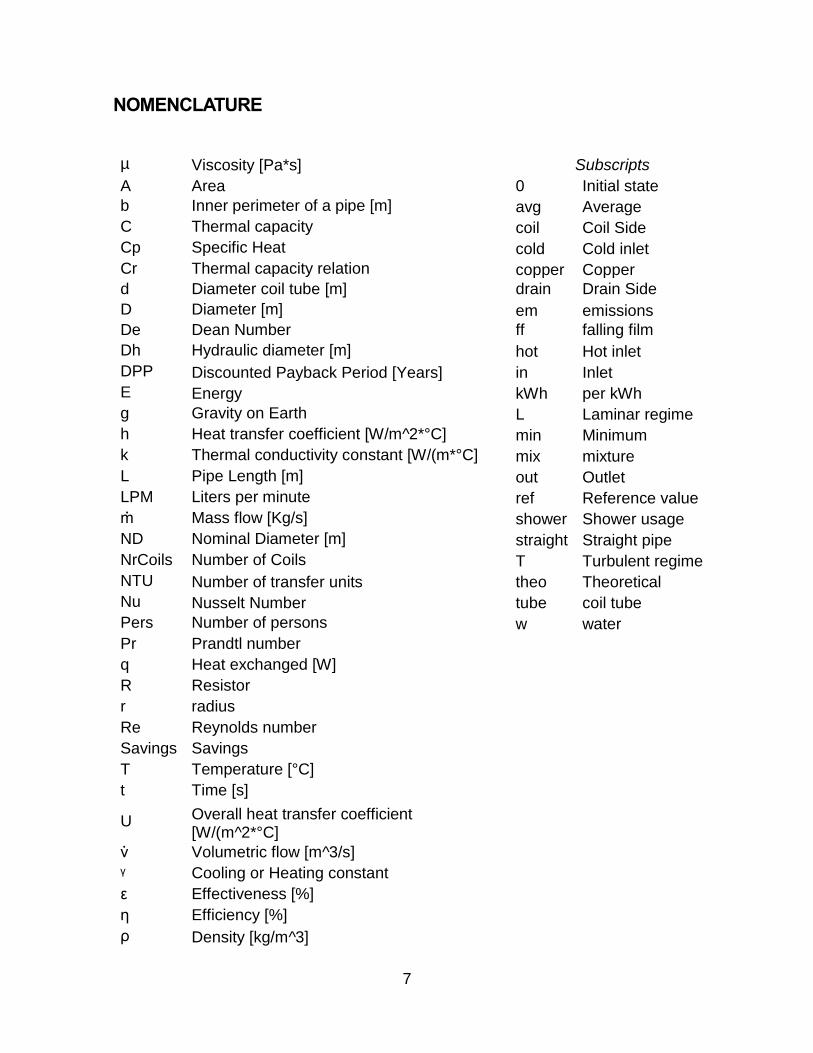
NOMENCLATURE

µ Viscosity [Pa*s] Subscripts

A Area 0 Initial state

b Inner perimeter of a pipe [m] avg Average

C Thermal capacity coil Coil Side

Cp Specific Heat cold Cold inlet

Cr Thermal capacity relation copper Copper

d Diameter coil tube [m] drain Drain Side

D Diameter [m] em emissions

De Dean Number ff falling film

Dh Hydraulic diameter [m] hot Hot inlet

DPP Discounted Payback Period [Years] in Inlet

E Energy kWh per kWh

g Gravity on Earth L Laminar regime

h Heat transfer coefficient [W/m^2*°C] min Minimum

k Thermal conductivity constant [W/(m*°C] mix mixture

L Pipe Length [m] out Outlet

LPM Liters per minute ref Reference value

m Mass flow [Kg/s] shower Shower usage

ND Nominal Diameter [m] straight Straight pipe

NrCoils Number of Coils T Turbulent regime

NTU Number of transfer units theo Theoretical

Nu Nusselt Number tube coil tube

Pers Number of persons w water

Pr Prandtl number

q Heat exchanged [W]

R Resistor

r radius

Re Reynolds number

Savings Savings

T Temperature [°C]

t Time [s]

U Overall heat transfer coefficient [W/(m^2*°C]

v Volumetric flow [m^3/s]

ᵞ Cooling or Heating constant

ε Effectiveness [%]

η Efficiency [%]

ρ Density [kg/m^3]

8

1 INTRODUCTION

Buildings account for up to 32% of the total energy use in the world. Different studies

have tried to calculate the impact of the built environment on the daily consumptions.

The influence differs from country to country, but it establishes a clear fact of the

importance of the buildings in the resource consumption of a nation.

In Canada, residential usage of energy and water accounts for 17% of the whole

consumption of the country (Leidl & David Lubitz 2009). The domestic sector in the

UK use 23% of the total consumption while in Hong Kong, it is determined to be 17%

(McNabola & Shields 2013). Households are responsible for almost 32% of the

energy consumed in Poland (Słyś & Kordana 2014).

The energy is used in several applications in residential buildings. The major

component of the consumption is directly linked to space heating, space cooling,

and water heating systems. Studies state that 51.9% of the energy used for these

applications, represent 55.7% of the costs and are responsible for 50.4% of the

greenhouse gas (GHG) emissions of the sector (Ni et al. 2012).

People are not aware of the fact that the energy consumption in the sector is high.

Just in Sweden, the Swedish Energy Agency (2014) estimates that in 2012, the

domestic household sector utilized over 46 TWh of district heating. It is important to

emphasize that 1 TWh is a lot of energy, putting it into perspective; 1 MWh can heat

a small house in Sweden for a couple of weeks. Despite that from the exergy point

of view, it is different to have electrical energy and thermal energy. It can be said

that all the Swedish Railways, subways and trams could be operated for 5 months

with just 1 TWh as an order of magnitude (Vattenfall 2015).

1.1 Heat generation in buildings

The previous statement says that space heating and water heating are the major

components of the consumptions in buildings. More studies support this statement

showing that, for example, in Canada, 57% of the energy is used for space heating

and 24% for water heating (representing almost 4% of the national energy demand).

The annual costs per household for 28 GJ were estimated at 2615 SEK2014 ($CAN

400) for gas water heaters and 4572 SEK2014 ($CAN 700) for electric one (Leidl &

David Lubitz 2009). For the UK, the percentage is almost the same accounting 26%

of the domestic energy consumption in water heating (McNabola & Shields 2013).

Different technologies have been applied to meet these demands: gas, oil, coal,

electric boilers, district heating, and others. In Sweden 2013, 51% of the energy in

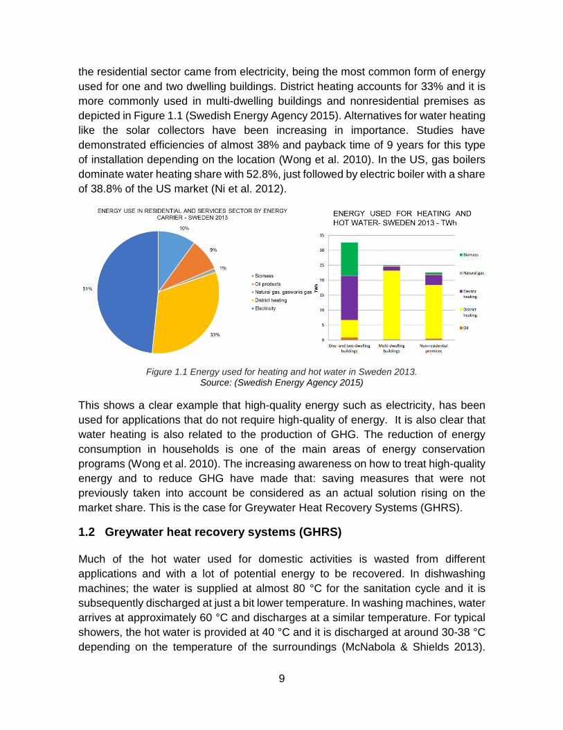
9

the residential sector came from electricity, being the most common form of energy

used for one and two dwelling buildings. District heating accounts for 33% and it is

more commonly used in multi-dwelling buildings and nonresidential premises as

depicted in Figure 1.1 (Swedish Energy Agency 2015). Alternatives for water heating

like the solar collectors have been increasing in importance. Studies have

demonstrated efficiencies of almost 38% and payback time of 9 years for this type

of installation depending on the location (Wong et al. 2010). In the US, gas boilers

dominate water heating share with 52.8%, just followed by electric boiler with a share

of 38.8% of the US market (Ni et al. 2012).

Figure 1.1 Energy used for heating and hot water in Sweden 2013.

Source: (Swedish Energy Agency 2015)

This shows a clear example that high-quality energy such as electricity, has been

used for applications that do not require high-quality of energy. It is also clear that

water heating is also related to the production of GHG. The reduction of energy

consumption in households is one of the main areas of energy conservation

programs (Wong et al. 2010). The increasing awareness on how to treat high-quality

energy and to reduce GHG have made that: saving measures that were not

previously taken into account be considered as an actual solution rising on the

market share. This is the case for Greywater Heat Recovery Systems (GHRS).

1.2 Greywater heat recovery systems (GHRS)

Much of the hot water used for domestic activities is wasted from different

applications and with a lot of potential energy to be recovered. In dishwashing

machines; the water is supplied at almost 80 °C for the sanitation cycle and it is

subsequently discharged at just a bit lower temperature. In washing machines, water

arrives at approximately 60 °C and discharges at a similar temperature. For typical

showers, the hot water is provided at 40 °C and it is discharged at around 30-38 °C

depending on the temperature of the surroundings (McNabola & Shields 2013).

10

When the greywater is sent down the drain, the water still contains 80% to 90% of

the original thermal energy (Dieckmann 2012). These facts reconfirmed the energy

inefficiencies currently found in a typical household and highlight the opportunity of

systems such as GHRS.

Figure 1.2 Shape of a vertical Greywater Heat Exchanger (GHE).

A heat recovery system is basically a heat exchanger with two streams where on

one side, a “hot” fluid flows and exchanges heat with a cold fluid that comes in the

other stream. This concept has been applied for several years in building industry

for ventilation systems, recovering the waste heat from the exhaust air and transfer

it to fresh air. This concept applied for greywater is more recent and it is up until now

that is gaining recognition and penetration of the marketplace that until now, remains

low (Leidl & David Lubitz 2009).

The concept behind the GHRS is to preheat the water before it enters the hot water

heater to reduce the amount of energy required to heat it up to the control

temperature. As a description of the device, a conventional drain pipe is replaced by

a copper pipe with a secondary pipe coiled around the first one. Hot drain water is

drained through the inner pipe by gravity while fresh water flows through the

secondary pipe exchanging heat between them.

1.3 Types of Greywater Heat Exchangers

In the market, different technologies of greywater heat exchangers exist. The first

classification is in two types: Storage and on-demand. Storage systems are

submerged copper exchangers in a fresh water tank. The drain water flows through

the copper exchanger heating up the water in the tank. On-demand devices use the

drain water that flows down the inner pipe and the incoming fresh water that flows

11

through an external pipe (Dieckmann 2012). From the on-demand devices, three

types can be studied and the temperature efficiency can be defined as:

𝜂𝑇 =𝑇𝑝𝑟𝑒ℎ𝑒𝑎𝑡𝑒𝑑 − 𝑇𝑐𝑜𝑙𝑑𝑇𝑤𝑎𝑠𝑡𝑒𝑤𝑎𝑡𝑒𝑟 − 𝑇𝐶𝑜𝑙𝑑

(1.1)

Where Tpreheated is the preheated fresh water leaving the greywater heat exchange,

Tcold is the temperature of fresh water entering the GHE and Twastewater is the hot drain

water.

1.3.1 Vertical heat exchangers

The first one is known as Vertical heat exchangers. This ones are basically a vertical

pipe that is installed in the vertical sewer stack producing a falling film effect on the

drain side. A helical coil is located around the drain pipe in which the fresh water

flows. The heat is exchanged between the inner pipe and the surrounding helical coil

in a process that will be explained further in chapter 3 of the present study. In the

market, several dimensions of heat exchangers exist with different nominal

diameters, lengths and number of coils (ReneWABILITY 2016). The effectiveness of

heat transfer of these devices varies for length, diameters, the number of coils and

other. Values in the range from 30-70% can be achieved (Collins et al. 2013). The

order of magnitude for the length of the vertical heat exchangers is around 0.9-1.5

meters for residential applications (Leidl & David Lubitz 2009).

1.3.2 Horizontal heat exchangers

Horizontal heat exchangers are installed in the collecting sewer pipes of all the

outgoing water of a building. Freshwater flows through a pipe in contact with the

drain pipe. The system is insulated to ensure that most of the heat goes to preheat

the incoming cold water. These devices usually have low temperatures which require

large heat exchanger to compensate this fact. The average efficiency of these

systems is estimated around 20% (Korpar Malmström 2015).

1.3.3 Shower heat exchangers

Shower heat exchangers are units located in the discharge of the shower. The floor

of the shower is changed for a heat exchanger configuration in which the incoming

cold water is preheated with the shower water flowing through the drain. Different

configuration and specification are available on the market. Effectiveness values

around 45% can be achieved according to McNabola & Shields (2013).

12

1.4 Project goals

The main objectives of the present master’s thesis are to:

Provide a better understanding of the fluid mechanics involved on the Vertical

greywater heat exchangers

Establish the basis of a heat transfer model that represents the physics of the

vertical greywater heat exchangers.

Analyze the potential of the technology for domestic households.

Study a methodology to perform an economic potential analysis of the

technology for a single household and multi-dwelling housing.

1.5 Project boundaries

The present project will focus on the analysis of vertically oriented greywater heat

exchangers. Two main fields will be subject to study: the heat transfer modeling of

the GHRS units and the potential implementation of the technology in residential

households from an economic perspective.

This heat transfer model will take a look at the available literature to describe the

phenomena of the vertical heat exchangers and a heat transfer model will be

proposed. A review on falling film effects and the secondary flow originated on the

flow through helical coils will be explained.

For the potential of implementation, this work will take a general look at the topic

from an economic perspective. Several conditions influencing this potential will be

explained. The economic results are proposed to evaluate the potential from a

general point of view and to understand the order of magnitude for the technology

and not as a market study.

This project will focus on the implementation on single-dwelling households with

electric boilers and the implication of low energy prices as it is the case with district

heating. For multi-dwelling housing, a short analysis on the potential of the

technology will be performed.

13

2 LITERATURE REVIEW

Greywater heat recovery system is a growing technology that has shown several

cost-efficient benefits to increase the energy efficiency. The literature on the field

has become available and in this chapter, it is intended to describe some of the most

relevant articles/thesis/reports available that were important for the development of

the present thesis. As stated before, the present thesis studies two main fields: the

heat transfer modeling of the GHRS units and the potential implementation of the

technology in residential households. To perform this, literature in both fields was

required.

Manouchehri (2015) focused on experimental correlation to simulate GHRS

performance in buildings. In addition, a heat transfer model was presented to predict

the performance of GHRS that operates under equal flow conditions and explains

concepts of the technology. This model was used as a base for the methodology

applied to the present project. Collins et al. (2013) executed tests under the

Canadian Standard CSA B55.1 to achieve characteristic effectiveness curves of

different GHRS units at different equal flow conditions. Zaloum et al. (2007) present

a detailed explanation of the arrangement and test procedure for eight units to obtain

their characteristic curves based on experimental data.

On the fluid mechanics of the GHRS units, a lot of works have been pointing out the

falling film condition and the secondary flow generated on helical coils. The falling

film effect is specially developed by Prost et al. (2006). The flow conditions inside a

helical coil have been the subject of study for numerous authors (Naphon &

Wongwises 2006; Collins et al. 2013; Wallin & Claesson 2014; Austen & Soliman

1988; Jayakumar et al. 2008; Janssen & Hoogendoorn 1978; Kozo & Yoshiyuki

1988; Rogers & Mayhew 1964).

Daniel Słyś and Sabina Kordana (2014) performed a financial analysis of the

implementation of GHRS in residential households. It presented a calculation model

that allows to estimate the Payback time of units under the influence of different

usage parameters.

The water usage pattern was studied by different authors (Opitz et al. 1999; Lallana

et al. 2001; Athuraliya et al. 2012; Blokker et al. 2010). Athuraliya et al. (2012) and

Blokker et al. (2010) report the different water usage behavior and patterns of

residential households and how to simulate them for Australia and the Netherlands,

respectively.

14

Additionally, several authors (Wong et al. 2010) (Ni et al. 2012) (McNabola & Shields

2013) (Leidl & David Lubitz 2009) (Dieckmann 2012) studied the impact of buildings

in the energy share and the potential of greywater to improve energy efficiency in

buildings.

Some of the findings and statement of these and other authors are going to be

developed further during the present work.

15

3 FLUID MECHANICS ANALYSIS

Greywater heat exchangers (GHE) have mainly two streams, coil-side (cold water)

and drain-side (drain water), as previously explained in chapter 1. The fluid

mechanics of both streams is the subject of study in this section in order to

understand the process inside the system. The GHE are generally ruled by two flow

phenomena. The first one is known as falling film effect and it rules over the drain-

side of the unit. Second, the flow through a helical coil for the cold water that it is

going to be heated up. This chapter will make a review of some of the principles that

rule these effects to provide the reader with a deeper understanding of the theory of

greywater heat exchangers.

3.1 Falling film effect

The falling film effect is the development of a layer of fluid in the boundaries of a

plate or pipe. For the subject of study, vertical oriented GHE use the effect of the

falling film to form an annular film inside the pipe (Figure 3.1) by gravity and it is one

of the main characteristics of this kind of vertically oriented units.

Figure 3.1 Aspect simulation of a full wetting falling film in a GHRS. Source: (Author)

This effect has several characteristics that are valuable for the GHRS performance.

As a starting point, the falling film effect maximizes the contact area between the

falling fluid (water for this purpose) and the inside area of the copper pipe. This

maximization of surface represents an increase of the heat transfer surface area

16

resulting in bigger heat transfer rates compared to the performance of horizontally

oriented as shown in Figure 3.2. With the equation 3.1, it is clear that bigger Areas

(A) achieve higher transfer rates.

�� = ℎ ∗ 𝐴 ∗ (𝑇ℎ − 𝑇𝑐) (3.1)

Furthermore, falling film effect minimizes the thickness of the layer of fluid which heat

is conducted till the boundary of the pipe. Afterward, this heat is convected to the

inner wall of the pipe (Manouchehri 2015). This refers to the phenomena that in the

case of a completely filled pipe, the heat of the fluid at the center has to be

transferred to the boundary layer in order to be transferred to the pipe. Turning the

heat transfer mechanism less effective than with this thin layer of fluid at the annulus.

Figure 3.2 Falling film formation in vertical oriented GHRS (Left) and fluid accumulation in horizontal oriented GHRS (right).

Source: (Author)

3.1.1 Falling Film Reynolds

The Reynolds number is a dimensionless quantity that measures the ratio of inertial

forces to viscous forces in the fluid (3.2). At small Reynolds numbers, viscous forces

are strong enough to keep the fluid in the laminar regime but for large numbers the

inertial forces are leading the relationship, therefore it flows in a turbulent regime

(Cengel & Cimbala 2006).

𝑅𝑒 =𝐼𝑛𝑒𝑟𝑡𝑖𝑎𝑙 𝐹𝑜𝑟𝑐𝑒𝑠

𝑉𝑖𝑠𝑐𝑜𝑢𝑠 𝐹𝑜𝑟𝑐𝑒𝑠 (3.2)

To estimate when this transition will happen, the concept of critical Reynolds shows

up. Collins et al. (2013) used the correlation for falling films on the surface of vertical

plates of Incropera et al. (2007) for GHE where it is established that:

17

𝑅𝑒𝑐𝑟𝑖𝑡𝑖𝑐𝑎𝑙𝑓𝑓 = 1800 (3.3)

𝑅𝑒𝑓𝑓 =4 ∗ mdrainµdrain ∗ b

(3.4)

Where b as the inner perimeter of the drain pipe.

3.1.2 Falling Film Heat Transfer Coefficient

Several correlations estimate the heat transfer coefficient at the falling film has been

developed by different authors. Prost et al. (2006) present a compilation of different

dimensionless heat transfer coefficient correlations. For the purpose of this work the

correlation of McAdams et al. (1940 Cited by Prost et al. 2006) on its non-

dimensionless form (3.5) is selected.

ℎ𝑓𝑓 = 0.01 ∗ 𝑅𝑒𝑑𝑟𝑎𝑖𝑛

13 ∗ 𝑃𝑟

𝑑𝑟𝑎𝑖𝑛

13 ∗ (

𝑘𝑑𝑟𝑎𝑖𝑛3 ∗ 𝑔 ∗ ρ𝑑𝑟𝑎𝑖𝑛

2

µ𝑑𝑟𝑎𝑖𝑛2 )

13

(3.5)

Where:

Redrain Reynolds number in the drain pipe

Prdrain Prandtl number

kdrain Thermal conductivity of the fluid [W/(m* °C)]

g Gravity [m/s^2]

ρdrain Fluid density [kg/m^3]

µdrain Dynamic viscosity [Pa*s]

The equation 3.5 was performed for water falling inside copper tubes and it is valid

for 1600 < Re < 50 000. For the different GHRS units available in the market, this

range works on their normal operation. The minimum volumetric flow required to

achieve this range is presented in table 3-1 for three different nominal diameters of

commercial GHE.

Nominal Diameter

[m]

V minimum [L/min]

0.05 3.21

0.08 5.24

0.10 6.61 Table 3-1 Minimum flow required to fulfill the range of McAdams correlation.

18

3.2 Flow through a helical coil

The second stream of study on the GHRS units it is the one through the outside coil.

Several authors (Naphon & Wongwises 2006; Collins et al. 2013; Wallin & Claesson

2014; Austen & Soliman 1988; Jayakumar et al. 2008; Janssen & Hoogendoorn

1978; Kozo & Yoshiyuki 1988; Rogers & Mayhew 1964) and many others have been

studied the phenomena of the flow through helical coils. A lot of information from the

experimental and theoretical side have been the subject of study. Nevertheless, it

still a complicated process and it is one of the bigger challenges for the study of

GHRS.

3.2.1 Helical Coil Reynolds Number

It is known that the centrifugal forces acting in the flow through helical coils generate

secondary flows (Kozo & Yoshiyuki 1988) (Janssen & Hoogendoorn 1978) (Austen

& Soliman 1988) as shown in figure 3.3. This fact increases the heat transfer

coefficient significantly in comparison with straight pipes. One of the main

consequences of the effect is that the transition to turbulent regime is achieved at

higher Reynolds number than in straight pipes (Collins et al. 2013) (Jayakumar et al.

2008).

Figure 3.3 Velocity contours [m/s] at different planes along the helical coil. Source: (Jayakumar et al. 2008)

In figure 3.3, the velocity contour alongside the helical coil is shown. At the inlet of

the coil, the velocity contour is homogenous and it does not present major

19

disturbances. This situation changes drastically inside the coil where due the effect

of the secondary flow, the velocity contour presents different values alongside the

helical coil.

Shah & Joshi (1987 cited by Collins et al. 2013) establish that the critical Reynolds

for helical coils is:

𝑅𝑒𝑐𝑟𝑖𝑡𝑖𝑐𝑎𝑙𝑐𝑜𝑖𝑙 = 2300 ∗ (1 + (12 ∗ √

𝑑𝑡𝑢𝑏𝑒𝐷𝑐𝑜𝑖𝑙

)) (3.6)

Where dtube is the diameter of the tube and Dcoil is the diameter of the coil. This critical

Reynolds number varies from 10,000-13,000 for standardized tubes of 3/8” copper

Type L with a nominal diameter of GHRS from 0.05-0.1 [m]. Reynolds number can

be calculated with Incropera et al. (2007) for pipes where Dh_tube is the hydraulic

diameter of the tube.

𝑅𝑒𝑐𝑜𝑖𝑙 =4 ∗ ��𝑐𝑜𝑖𝑙

µ𝑐𝑜𝑖𝑙 ∗ 𝜋 ∗ 𝐷ℎ𝑡𝑢𝑏𝑒 (3.7)

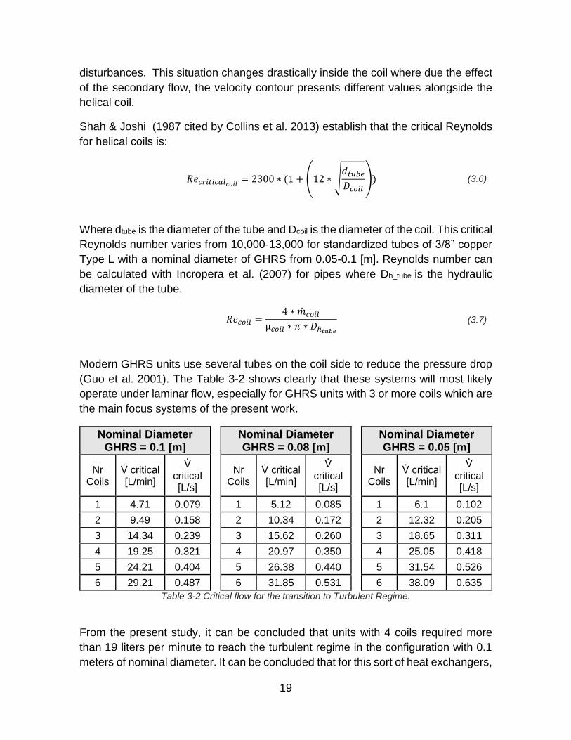
Modern GHRS units use several tubes on the coil side to reduce the pressure drop

(Guo et al. 2001). The Table 3-2 shows clearly that these systems will most likely

operate under laminar flow, especially for GHRS units with 3 or more coils which are

the main focus systems of the present work.

Nominal Diameter GHRS = 0.1 [m]

Nominal Diameter GHRS = 0.08 [m]

Nominal Diameter GHRS = 0.05 [m]

Nr Coils

V critical [L/min]

V critical [L/s]

Nr

Coils V critical [L/min]

V critical [L/s]

Nr

Coils V critical [L/min]

V critical [L/s]

1 4.71 0.079 1 5.12 0.085 1 6.1 0.102

2 9.49 0.158 2 10.34 0.172 2 12.32 0.205

3 14.34 0.239 3 15.62 0.260 3 18.65 0.311

4 19.25 0.321 4 20.97 0.350 4 25.05 0.418

5 24.21 0.404 5 26.38 0.440 5 31.54 0.526

6 29.21 0.487 6 31.85 0.531 6 38.09 0.635

Table 3-2 Critical flow for the transition to Turbulent Regime.

From the present study, it can be concluded that units with 4 coils required more

than 19 liters per minute to reach the turbulent regime in the configuration with 0.1

meters of nominal diameter. It can be concluded that for this sort of heat exchangers,

20

they will always operate in the laminar regime under standard conditions. For units

with just 1 coil, the regime transition is easily achievable under the normal operation

conditions and the turbulent correlation must be applied.

3.2.2 Dean & Nusselt numbers

The secondary flow increases the heat transfer and in order to gain a better

understanding of the heat transfer and the hydrodynamics, the Dean & Nusselt

number should be studied. Firstly, the dimensionless characteristic known as Dean

Number is fundamentally important for this process. It can be defined as Janssen &

Hoogendoorn (1978) proposed:

𝐷𝑒 = 𝑅𝑒𝑐𝑜𝑖𝑙 ∗ 𝑠𝑞𝑟𝑡 (𝑑𝑡𝑢𝑏𝑒𝐷𝑐𝑜𝑖𝑙

) (3.8)

It is a number that relates the Reynolds number with the diameters of the geometry

of the coil, where Recoil is the Reynolds number, dtube the diameter of the tube and

Dcoil the diameter of the coil.

Secondly, the Nusselt number is a ratio of convective to conductive heat transfer at

the boundary layer of the fluid. It is equal to the dimensionless temperature gradient

at the surface layer and exposed a measure of the convection that occurs there

(Incropera et al. 2007).

In the literature, there are several different correlations for the Nusselt number in

laminar and/or turbulent regimes. For the purpose of the present work, these

correlations were evaluated in order to find out which relation displayed better results

for the GHRS units. This analysis will be developed further in chapter 5 during the

model validation. It is important to remark that these correlations are based on

cylindrical pipes that for the case of GHRS is not that common. For this reason, these

correlations are applied with the purpose to evaluate performance within an

academic approach; it is not meant to be used as design parameters.

3.2.2.1 Laminar

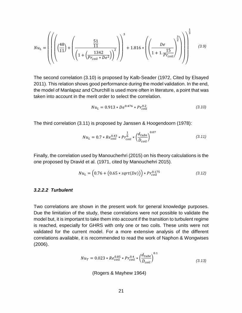
The correlation in equation 3.9 is from Manlapaz and Churchill (1980, cited by

Austen & Soliman 1988). This equation displayed significantly more accurate results

than the other correlations and for that reason, it was selected for the heat transfer

model of the GHRS. (To find out these results, refer to chapter 5).

21

𝑁𝑢𝐿 =

(

(

(

(48

11) +

(

5111

(1 + (1342

𝑃𝑟𝑐𝑜𝑖𝑙 ∗ 𝐷𝑒2))

2

)

)

3

+ 1.816 ∗

(

(

𝐷𝑒

1 + 1.15𝑃𝑟𝑐𝑜𝑖𝑙

)

32

)

)

)

13

(3.9)

The second correlation (3.10) is proposed by Kalb-Seader (1972, Cited by Elsayed

2011). This relation shows good performance during the model validation. In the end,

the model of Manlapaz and Churchill is used more often in literature, a point that was

taken into account in the merit order to select the correlation.

𝑁𝑢𝐿 = 0.913 ∗ 𝐷𝑒0.476 ∗ 𝑃𝑟𝑐𝑜𝑖𝑙

0.2 (3.10)

The third correlation (3.11) is proposed by Janssen & Hoogendoorn (1978):

𝑁𝑢𝐿 = 0.7 ∗ 𝑅𝑒𝑐𝑜𝑖𝑙

0.43 ∗ 𝑃𝑟𝑐𝑜𝑖𝑙

16 ∗ (

𝑑𝑡𝑢𝑏𝑒𝐷𝑐𝑜𝑖𝑙

)0.07

(3.11)

Finally, the correlation used by Manoucherhri (2015) on his theory calculations is the

one proposed by Dravid et al. (1971, cited by Manouchehri 2015).

𝑁𝑢𝐿 = (0.76 + (0.65 ∗ 𝑠𝑞𝑟𝑡(𝐷𝑒))) ∗ 𝑃𝑟𝑐𝑜𝑖𝑙0.175 (3.12)

3.2.2.2 Turbulent

Two correlations are shown in the present work for general knowledge purposes.

Due the limitation of the study, these correlations were not possible to validate the

model but, it is important to take them into account if the transition to turbulent regime

is reached, especially for GHRS with only one or two coils. These units were not

validated for the current model. For a more extensive analysis of the different

correlations available, it is recommended to read the work of Naphon & Wongwises

(2006).

𝑁𝑢𝑇 = 0.023 ∗ 𝑅𝑒𝑐𝑜𝑖𝑙

0.85 ∗ 𝑃𝑟𝑐𝑜𝑖𝑙0.4 ∗ (

𝑑𝑡𝑢𝑏𝑒𝐷𝑐𝑜𝑖𝑙

)0.1

(3.13)

(Rogers & Mayhew 1964)

22

𝑁𝑢𝑠𝑡𝑟𝑎𝑖𝑔ℎ𝑡 = 0.023 ∗ 𝑅𝑒𝑐𝑜𝑖𝑙

45 ∗ 𝑃𝑟𝑐𝑜𝑖𝑙

ᵞ

𝑁𝑢𝑇4 = 𝑁𝑢𝑠𝑡𝑟𝑎𝑖𝑔ℎ𝑡 ∗ (1 + 3.4 ∗ (𝑑𝑡𝑢𝑏𝑒𝐷𝑐𝑜𝑖𝑙

)) (3.14)

(Incropera et al. 2007)

Where ᵞ is 0.4 for heating and 0.3 for cooling processes.

3.2.3 Heat Transfer coefficient of helical coils

The heat transfer coefficient is shown in equation 3.15, where hcoil is the heat transfer

coefficient, Nu is the Nusselt number depending on the regime and the correlation

used, kcoil is the thermal conductivity of the fluid flowing through the coil and dtube is

the diameter of the tube.

ℎ𝑐𝑜𝑖𝑙 = 𝑁𝑢 ∗𝐾𝑐𝑜𝑖𝑙𝑑𝑡𝑢𝑏𝑒

(3.15)

23

4 HEAT TRANSFER MODEL

The heat transfer model is a starting point to predict the theoretical performance of

different GHRS units. The current model is based on the ε-NTU method from

Incropera et al. (2007) following some of the theory basis exposed by Manouchehri

(2015) and modified by the author of the present work. On this chapter, a heat

transfer methodology is proposed and the different steps of it are explained.

The ε-NTU method use ε as a characteristic parameter and it is defined in the

equation 4.1 as the ratio of the real heat transfer rate (q) with the maximum possible

heat transfer rate (qmax) (Incropera et al. 2007).

𝜀 =𝑞

𝑞𝑚𝑎𝑥 (4.1)

The effectiveness (ε) and the actual heat transfer rate (q) are two of the final

objectives of the heat transfer model. As the model presented by Manouchehri

(2015) based on Incropera et al. (2007), the use of a thermal resistor to describe the

heat transfer process is a simplified way to solve the problem as shown in figure 4.1.

Figure 4.1 Thermal resistors of the heat transfer model. Source: (Author)

Where the overall heat transfer coefficient for a GHRS can be found with a network

of thermal resistance in series configuration as explained by the equation 4.2.

1

𝑈𝐴= 𝑅𝑡𝑜𝑡𝑎𝑙 = 𝑅1 + 𝑅2 + 𝑅3 + 𝑅4 + 𝑅5 (4.2)

A schematic flow diagram of the whole model proposed is shown in APPENDIX A.

Tff Tsurfdrain Tinterference

Drain-side

Tinterference

Coil-side

Tinnercoil Tcoil

R1 R2 R3 R4 R5

CONVECTION

Falling Film

CONDUCTION

Drain-side

INTERFERENCE CONDUCTION

Coil-sideCONVECTION

Helical Coil

24

4.1 Inputs of the model

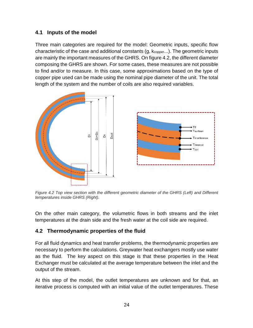
Three main categories are required for the model: Geometric inputs, specific flow

characteristic of the case and additional constants (g, kcopper...). The geometric inputs

are mainly the important measures of the GHRS. On figure 4.2, the different diameter

composing the GHRS are shown. For some cases, these measures are not possible

to find and/or to measure. In this case, some approximations based on the type of

copper pipe used can be made using the nominal pipe diameter of the unit. The total

length of the system and the number of coils are also required variables.

Figure 4.2 Top view section with the different geometric diameter of the GHRS (Left) and Different temperatures inside GHRS (Right).

On the other main category, the volumetric flows in both streams and the inlet

temperatures at the drain side and the fresh water at the coil side are required.

4.2 Thermodynamic properties of the fluid

For all fluid dynamics and heat transfer problems, the thermodynamic properties are

necessary to perform the calculations. Greywater heat exchangers mostly use water

as the fluid. The key aspect on this stage is that these properties in the Heat

Exchanger must be calculated at the average temperature between the inlet and the

output of the stream.

At this step of the model, the outlet temperatures are unknown and for that, an

iterative process is computed with an initial value of the outlet temperatures. These

25

outlet temperatures would be recalculated through the calculation until the outlet

temperatures converge with the real output temperatures of the exchanger.

Using the software Engineering Equation Solver the properties of specific heat,

dynamic viscosity, Prandtl number, thermal conductivity and fluid density are

calculated for water within a range of 0<T<60 [°C] and 1 atmosphere (Table 0-1

APPENDIX A).

A fifth order polynomial fit is applied and the following correlations are obtained as

result:

The specific heat in [kJ/ kg*K]:

𝐶𝑝𝑑𝑟𝑎𝑖𝑛 = 4.22783901 − 0.00783849467 ∗ 𝑇𝑎𝑣𝑔 + 0.00052713434 ∗ 𝑇𝑎𝑣𝑔2

− 0.0000169714919 ∗ 𝑇𝑎𝑣𝑔3 + 2.62003476𝐸 − 07 ∗ 𝑇𝑎𝑣𝑔

4

− 1.56365456𝐸 − 09 ∗ 𝑇𝑎𝑣𝑔5

(4.3)

The dynamic viscosity [kg/ m*s]:

µ = 0.0017922553 − 0.0000619423739 ∗ 𝑇𝑎𝑣𝑔 + 0.00000161169391 ∗ 𝑇𝑎𝑣𝑔2

− 3.12027493𝐸 − 08 ∗ 𝑇𝑎𝑣𝑔3 + 3.75757478𝐸 − 10 ∗ 𝑇𝑎𝑣𝑔

4

− 2.00244305𝐸 − 12 ∗ 𝑇𝑎𝑣𝑔5

(4.4)

The dimensionless Prandtl number:

𝑃𝑟 = 13.8366012 − 0.551920297 ∗ 𝑇𝑎𝑣𝑔 + 0.0163242036 ∗ 𝑇𝑎𝑣𝑔2

− 0.000354310865 ∗ 𝑇𝑎𝑣𝑔3 + 0.00000465354551 ∗ 𝑇𝑎𝑣𝑔

4

− 2.63157066𝐸 − 08 ∗ 𝑇𝑎𝑣𝑔5

(4.5)

Thermal conductivity [W/ m*K]:

𝑘 = 0.547511995 + 0.00204429925 ∗ 𝑇𝑎𝑣𝑔 − 0.0000044046946 ∗ 𝑇𝑎𝑣𝑔2

− 6.41854726𝐸 − 08 ∗ 𝑇𝑎𝑣𝑔3 − 4.68031789𝐸 − 10 ∗ 𝑇𝑎𝑣𝑔

4

+ 8.66907284𝐸 − 12 ∗ 𝑇𝑎𝑣𝑔5

(4.6)

Fluid density [kg/ m^3]:

𝜌 = 999.8297 + 0.0789410566 ∗ 𝑇𝑎𝑣𝑔 − 0.00982564195 ∗ 𝑇𝑎𝑣𝑔2

+ 0.00011599958 ∗ 𝑇𝑎𝑣𝑔3 − 0.00000120708114 ∗ 𝑇𝑎𝑣𝑔

4

+ 5.95968898𝐸 − 09 ∗ 𝑇𝑎𝑣𝑔5

(4.7)

26

It is important to remark that all of these properties have to be calculated separately

for each stream, the coil side and the drain side.

4.3 Thermal Capacities

The thermal capacities are calculated through the standard methodology. It is

essential that for the capacity of the coil, the number of coils (Nrcoils) must be taken

into account. The flow inside each of the coils is considered to be equal for all of

them and mcoil represents the mass flow on each coil. With the values of the equation

4.8, Cmin and Cmax can be assigned and determined the relation of Cr following

equation 4.9.

𝐶𝑑𝑟𝑎𝑖𝑛 = ��𝑑𝑟𝑎𝑖𝑛 ∗ 𝐶𝑝𝑑𝑟𝑎𝑖𝑛

𝐶𝑐𝑜𝑖𝑙 = ��𝑐𝑜𝑖𝑙 ∗ 𝐶𝑝𝑐𝑜𝑖𝑙 ∗ 𝑁𝑟𝐶𝑜𝑖𝑙𝑠 (4.8)

𝐶𝑟 =𝐶𝑚𝑖𝑛𝐶𝑚𝑎𝑥

(4.9)

4.4 Convection Falling Film – R1

The falling film effect was explained in Chapter 3. Following that methodology, the

first thermal resistance is determined using the heat transfer coefficient (hff)

established by equation 3.4.

𝑅1 =1

ℎ𝑓𝑓 ∗ 2 ∗ 𝜋 ∗ (𝐷12) ∗ 𝐿

(4.10)

4.5 Conduction Drain Pipe – R2

The conduction process that occurs on the pipe is estimated using the equation 4.11

in which the relation of external and internal diameter is used. L is the length of the

pipe and kcopper is the thermal conductivity of copper which value for the normal

condition is approximately 401 [W/ m*K].

𝑅2 =

𝑙𝑛 (

𝐷22𝐷12

)

2 ∗ 𝜋 ∗ 𝐿 ∗ 𝑘𝑐𝑜𝑝𝑝𝑒𝑟

(4.11)

27

4.6 Contact Resistance – R3

The presence of an interface between the drain pipe and the coils can be simulated

through the theory of contact resistance propose by Incropera et al. (2007). In the

Greywater heat exchanger, a copper-copper interface is present.

Two surfaces will never form a perfect thermal contact when they are put together.

Roughness becomes important due the fact that it will always include gaps of air

between the surfaces as shown in figure 4.3. In a thermal contact resistance, the

heat follows two different paths: a conduction between the points of solid-to-solid

contact which is very effective and a convection through the air between the gaps in

which the mechanism of heat transfer performs poorly (Lienhard IV & Lienhard V

1986).

Figure 4.3 Heat transfer through contact plane between two solid surfaces.

Source: (Lienhard IV & Lienhard V 1986)

The main factors that influence the contact resistance are the roughness of the

surface, the material, the pressure at which the surface are forced together, the

interstitial fluid and the temperature of contact. Considering the greywater heat

exchangers, the contact resistant accounts for roughly a 6.24% (APPENDIX A: Table

A-2) of the total thermal resistance.

𝑅3 =1

ℎ𝐶 ∗ 𝐴 (4.12)

The coefficient of interfacial conductance (hc) has values of 10,000-25,000

[W/(m^2*K)] (Rohsenow & Hartnett 1973 cited by Lienhard IV & Lienhard V 1986).

A value of 25,000 [W/(m^2*K)] for the interfacial coefficient (hc) is used for the

present work.

28

For the Greywater heat exchanger, this interface presents contact discontinuity due

the fact of several coils pile together. For the present work, this contact resistance

was assumed to be the same alongside the unit, but it is important to remark the fact

that the heat transfer mechanism is less effective in the gaps between coils.

4.7 Conduction Coil Pipe – R4

Following the same methodology as section 4.5, the conduction on the coil pipe is

calculated with the equation 4.13 representing the resistor 4.

𝑅4 =

𝑙𝑛 (

𝐷42𝐷32

)

2 ∗ 𝜋 ∗ 𝐿𝑐𝑜𝑖𝑙 ∗ 𝑘𝑐𝑜𝑝𝑝𝑒𝑟

(4.13)

4.8 Convection Helical Coil – R5

The phenomena of the secondary flow originated in the helical coil was explained in

section 3.2. The thermal resistance for the convective heat of the flow through the

helical coil is calculated using the equation 4.14 where hcoil is defined by the equation

3.14.

𝑅5 =1

ℎ𝑐𝑜𝑖𝑙 ∗ 2 ∗ 𝜋 ∗ (𝐷42 ) ∗ 𝐿𝑐𝑜𝑖𝑙

(4.14)

4.9 NTU-Method

Once the different resistors have been calculated, the overall heat transfer coefficient

(U) and the heat transfer Area (A) is estimated using equation 4.15 with the total

resistor of equation 4.2. A table with the thermal resistors calculated and the

percentage of the total resistor can be found on the table A-2 of APPENDIX A.

𝑈𝐴 =1

𝑅𝑡𝑜𝑡𝑎𝑙 (4.15)

Following the methodology of Incropera et al. (2007) the number of transfer units

(NTU) is determined where Cmin is the minimum thermal capacity, it can be Ccoil or

Cdrain depending on the conditions.

𝑁𝑇𝑈 =𝑈𝐴

𝐶𝑚𝑖𝑛 (4.16)

29

The effectiveness is calculated in equation 4.17 for counterflow GHRS units. If the GHRS is installed in a parallel flow configuration a different relation must be used as presented in equation 4.18. It is important to remark, that higher values of effectiveness are achieved with the counterflow configuration and that is why the parallel configuration must be avoided.

𝜀𝑡ℎ𝑒𝑜_𝑐𝑜𝑢𝑛𝑡𝑒𝑟𝑓𝑙𝑜𝑤 =

1 − 𝑒𝑥𝑝(−𝑁𝑇𝑈(1 − 𝐶𝑟))

1 − 𝐶𝑟 ∗ 𝑒𝑥𝑝(−𝑁𝑇𝑈 ∗ (1 − 𝐶𝑟)) (4.17)

𝜀𝑡ℎ𝑒𝑜𝑝𝑎𝑟𝑎𝑙𝑙𝑒𝑙 =

1 − 𝑒𝑥𝑝(−𝑁𝑇𝑈(1 + 𝐶𝑟))

1 + 𝐶𝑟 (4.18)

The heat recovery (q) of the GHRS unit is evaluation using the qmax which is the

relation between the minimum thermal capacity and the two limit temperatures. This

value is applied alongside the effectiveness value to obtain q.

𝑞 = 𝜀𝑡ℎ𝑒𝑜 ∗ 𝐶𝑚𝑖𝑛 ∗ (𝑇𝑑𝑟𝑎𝑖𝑛𝑖𝑛 − 𝑇𝑐𝑜𝑖𝑙𝑖𝑛) (4.19)

Outlet temperatures are calculated using the expression 4.20 for both streams.

𝑇𝑐𝑜𝑖𝑙𝑜𝑢𝑡 = (𝑞

𝐶𝑐𝑜𝑖𝑙) + 𝑇𝑐𝑜𝑖𝑙𝑖𝑛

𝑇𝑑𝑟𝑎𝑖𝑛𝑜𝑢𝑡 = 𝑇𝑑𝑟𝑎𝑖𝑛𝑖𝑛 − (𝑞

𝐶𝑑𝑟𝑎𝑖𝑛)

(4.20)

30

5 MODEL VALIDATION

Models are an approximation of reality, therefore, it is important that the models are

well-founded and represent with a certain margin of error the phenomena it tries to

describe. For this process, the current heat transfer model was validated with the

empirical data available from Collins (2009) and the reference values from the

nominal effectiveness which are also available there. Collins (2009) performed tests

under different flow and standard conditions for different Greywater heat

exchangers. On this chapter, the validation process of the heat transfer model is

presented.

5.1 Nusselt Correlation

On this section different laminar Nusselt correlations (Section 3.2.2) were evaluated

in order to find out which relation displays better results. For the evaluation of the

flow through a helical coil, the correlations of (Eq. 3.8) Manlapaz and Churchill (1980,

cited by Austen & Soliman 1988); (Eq. 1.9) Karl-Saeder (1972, Cited by Elsayed

2011); (Eq. 3.10) Janssen & Hoogendoorn (1978) and (Eq.3.11) Dravid et al. (1971,

cited by Manouchehri 2015) were validated in order to look for the correlation that

gives the most accurate results.

Figure 5.1 Cumulative histogram frequencies of the Heat Recovery Error (Top) and effectiveness Error (Bottom) for different Nusselt Correlations.

31

A validation process with 54 different geometries was evaluated. The correlation of

Manlapaz & Churchill and Karl-Saeder outperformed the other correlations. For

Manlapaz & Churchill, 75.93% of the times the error in the heat recovery (q) is below

6.0% and 92.59% of the times is below 10%. For the Karl-Saeder case, the same

order of magnitude is achieved. For Janssen correlation, only 51.85% of the times

the error was below 10% which is not significantly accurate. Dravid et al. expression

obtain error below 10%, 85.19% of the times but the error was only below 6%,

46.30% of the times. A Cumulative Histogram of the frequencies is depicted in figure

5.1 and for the full table of results refer to the tables B-1 and B-2 of APPENDIX B.

For the present work, the correlation of Manlapaz & Churchill was used for the

current model due the results achieved in this section.

5.2 Standard Condition

On the validation process, the 54 models were evaluated and some of the results

are shown in table 5-1 (to see the full table of results refer to Table B-2 in APPENDIX

B).

The conditions for this validation test were 9 [L/min] of water flow in both streams,

inlet drain temperature of 36°C and inlet coil temperature of 8°C.

(COLLINS 2009) Manlapaz and Churchill

MODEL

No

min

al

Dia

me

ter

[m]

Le

ng

th [

m]

Eff

ecti

ve

ne

ss

[%]

Heat

Rec

ov

ery

[W

]

Eff

ecti

ve

ne

ss

[%]

Eff

ecti

ve

ne

ss

ER

RO

R [

%]

Heat

Rec

ov

ery

[W

]

Heat

Rec

ov

ery

ER

RO

R [

W]

R2-36 0.05 0.91 32.6% 5720 31.1% 4.73% 5430.13 5.07%

R2-48 0.05 1.22 37.8% 6540 37.7% 0.36% 6586.90 0.72%

R2-120 0.05 3.05 64.4% 10810 60.1% 6.63% 10526.35 2.62%

R3-36 0.08 0.91 38.7% 6790 38.4% 0.89% 6708.24 1.20%

R3-42 0.08 1.07 43.1% 7500 42.3% 1.97% 7390.78 1.46%

R3-120 0.08 3.05 67.8% 12060 67.5% 0.40% 11824.44 1.95%

R4-36 0.1 0.91 43.0% 7580 42.1% 2.10% 7363.98 2.85%

R4-108 0.1 2.74 69.6% 12120 68.6% 1.48% 12008.19 0.92%

R4-120 0.1 3.05 72.4% 12760 70.8% 2.18% 12403.49 2.79%

C3-84 0.08 2.13 56.3% 9720 56.9% 1.06% 9959.25 2.46%

C3-96 0.08 2.44 60.7% 10520 60.2% 0.83% 10538.24 0.17%

C3-120 0.08 3.05 66.4% 11570 65.4% 1.50% 11452.22 1.02%

C4-96 0.1 2.44 65.8% 11350 63.9% 2.95% 11180.78 1.49%

C4-108 0.1 2.74 68.9% 12010 66.5% 3.50% 11642.45 3.06%

C4-120 0.1 3.05 70.8% 11940 68.8% 2.78% 12053.73 0.95%

Table 5-1 Table of Errors for GHRS Units with 0.08 m of nominal diameter.

32

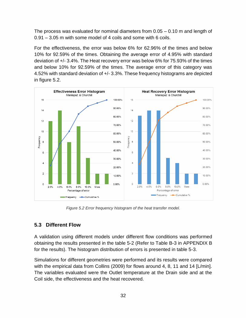
The process was evaluated for nominal diameters from 0.05 – 0.10 m and length of

0.91 – 3.05 m with some model of 4 coils and some with 6 coils.

For the effectiveness, the error was below 6% for 62.96% of the times and below

10% for 92.59% of the times. Obtaining the average error of 4.95% with standard

deviation of +/- 3.4%. The Heat recovery error was below 6% for 75.93% of the times

and below 10% for 92.59% of the times. The average error of this category was

4.52% with standard deviation of +/- 3.3%. These frequency histograms are depicted

in figure 5.2.

Figure 5.2 Error frequency histogram of the heat transfer model.

5.3 Different Flow

A validation using different models under different flow conditions was performed

obtaining the results presented in the table 5-2 (Refer to Table B-3 in APPENDIX B

for the results). The histogram distribution of errors is presented in table 5-3.

Simulations for different geometries were performed and its results were compared

with the empirical data from Collins (2009) for flows around 4, 8, 11 and 14 [L/min].

The variables evaluated were the Outlet temperature at the Drain side and at the

Coil side, the effectiveness and the heat recovered.

33

Table 5-2 Table of Error with different flows.

Percentage of error

Temp. Drain Out Temp. Coil Out Effectiveness Heat Recovery

Fre

quency

Cum

ula

tive

[%]

Fre

quency

Cum

ula

tive

[%]

Fre

quency

Cum

ula

tive

[%]

Fre

quency

Cum

ula

tive

[%]

2% 14 43.75% 11 34.38% 8 25.00% 8 25.00%

4% 9 71.88% 14 78.13% 7 46.88% 7 46.88%

6% 4 84.38% 2 84.38% 10 78.13% 9 75.00%

8% 2 90.63% 4 96.88% 2 84.38% 3 84.38%

10% 0 90.63% 1 100.00% 3 93.75% 2 90.63%

12% 2 96.88% 0 100.00% 2 100.00% 3 100.00%

More 1 100.00% 0 100.00% 0 100.00% 0 100.00%

Table 5-3 Histogram table of validation process with different flows.

RE

F.

Tem

p. D

rain

In

[°C

]

Tem

p. C

oil

In

[°C

]

Flo

w [LP

M]

(CO

LLIN

S 2

009)

[°C

]

MO

DE

L [°C

]

DIF

F. [°

C]

Err

or

[%]

(CO

LLIN

S 2

009)

[°C

]

MO

DE

L [°C

]

DIF

F. [°

C]

Err

or

[%]

(CO

LLIN

S 2

009)

[°C

]

MO

DE

L

DIF

F.

Err

or

[%]

(CO

LLIN

S 2

009)

[°C

]

MO

DE

L [W

]

DIF

F. [W

]

Err

or

[%]

35.7 8.1 3.99 19.1 19.84 -0.74 3.89% 24.6 23.91 0.69 2.80% 0.601 0.574 0.027 4.41% 4610 4395 215 4.67%

36.2 8.2 7.92 22.2 23.12 -0.92 4.14% 21.9 21.23 0.67 3.05% 0.492 0.467 0.025 5.06% 7600 7191 409 5.38%

36.1 8.0 10.84 23.5 24.39 -0.89 3.79% 20.4 19.66 0.74 3.62% 0.443 0.417 0.026 5.94% 9420 8810 610 6.48%

35.9 8.2 14.23 25.4 25.54 -0.14 0.53% 19.2 18.52 0.68 3.54% 0.396 0.374 0.022 5.51% 10860 10236 624 5.75%

35.9 8.2 4.16 15.8 15.83 -0.03 0.18% 28.4 28.24 0.16 0.57% 0.729 0.725 0.004 0.60% 5840 5803 37 0.63%

36.0 7.7 7.88 18.5 18.00 0.50 2.69% 25.3 25.66 -0.36 1.40% 0.624 0.636 -0.012 1.92% 9690 9854 -164 1.69%

36.0 8.0 10.73 20.1 19.50 0.60 2.96% 23.9 24.45 -0.55 2.30% 0.569 0.589 -0.020 3.53% 11900 12295 -395 3.32%

36.5 8.0 13.80 22 20.83 1.17 5.32% 23 23.62 -0.62 2.70% 0.527 0.550 -0.023 4.32% 14430 15016 -586 4.06%

36.0 7.8 4.06 20.1 18.61 1.49 7.41% 23.6 25.15 -1.55 6.55% 0.559 0.617 -0.058 10.31% 4450 4905 -455 10.22%

35.6 7.8 7.96 20.8 21.36 -0.56 2.69% 22.6 21.99 0.61 2.70% 0.531 0.512 0.019 3.56% 8180 7870 310 3.79%

35.5 7.7 10.63 22.7 22.55 0.15 0.65% 20.6 20.60 0.00 0.01% 0.464 0.466 -0.002 0.37% 9540 9557 -17 0.18%

36.3 7.9 14.03 24.6 24.27 0.33 1.33% 19.6 19.88 -0.28 1.42% 0.415 0.423 -0.008 2.04% 11500 11711 -211 1.84%

35.7 7.6 4.06 16.4 13.77 2.63 16.04% 27.3 29.49 -2.19 8.02% 0.7 0.780 -0.080 11.46% 5580 6188 -608 10.90%

35.7 8.1 8.45 17 16.61 0.39 2.29% 27.1 27.15 -0.05 0.18% 0.687 0.692 -0.005 0.67% 11160 11210 -50 0.44%

36.1 8.0 10.85 17.6 17.63 -0.03 0.17% 26.6 26.42 0.18 0.68% 0.662 0.657 0.005 0.76% 14050 13920 131 0.93%

35.7 7.6 13.77 17.6 18.33 -0.73 4.15% 25.8 24.93 0.87 3.38% 0.65 0.618 0.032 4.90% 17520 16618 902 5.15%

36.1 8.1 4.16 16.9 16.73 0.17 0.99% 27 27.42 -0.42 1.56% 0.677 0.692 -0.015 2.17% 5480 5598 -118 2.16%

36.1 8.0 7.79 19 19.18 -0.18 0.97% 25.1 24.87 0.23 0.92% 0.611 0.602 0.009 1.47% 9280 9154 126 1.36%

35.9 8.0 10.81 19.3 20.53 -1.23 6.36% 24.6 23.33 1.27 5.17% 0.594 0.551 0.043 7.26% 12450 11541 909 7.30%

36.1 7.7 14.09 20.8 21.65 -0.85 4.09% 23.7 22.09 1.61 6.79% 0.562 0.509 0.053 9.49% 15650 14135 1516 9.68%

36.2 8.3 3.97 15.5 13.67 1.83 11.81% 28.8 30.79 -1.99 6.91% 0.734 0.807 -0.073 9.98% 5640 6216 -576 10.20%

36.2 8.1 8.44 15.7 15.90 -0.20 1.27% 28.6 28.36 0.24 0.84% 0.732 0.722 0.010 1.31% 12080 11907 173 1.43%

35.8 7.9 11.23 16.2 16.73 -0.53 3.25% 27.7 26.94 0.76 2.76% 0.709 0.684 0.025 3.57% 15460 14885 575 3.72%

35.9 8.1 14.08 16 17.77 -1.77 11.06% 27.9 26.18 1.72 6.16% 0.711 0.652 0.059 8.31% 19400 17731 1669 8.60%

Heat RecoveryINITIAL PARAMETERS

R4-66

R4-120

Temp. Drain OUT Temp. Coil OUT Effectiveness

R2-60

R2-120

R3-54

R3-120

34

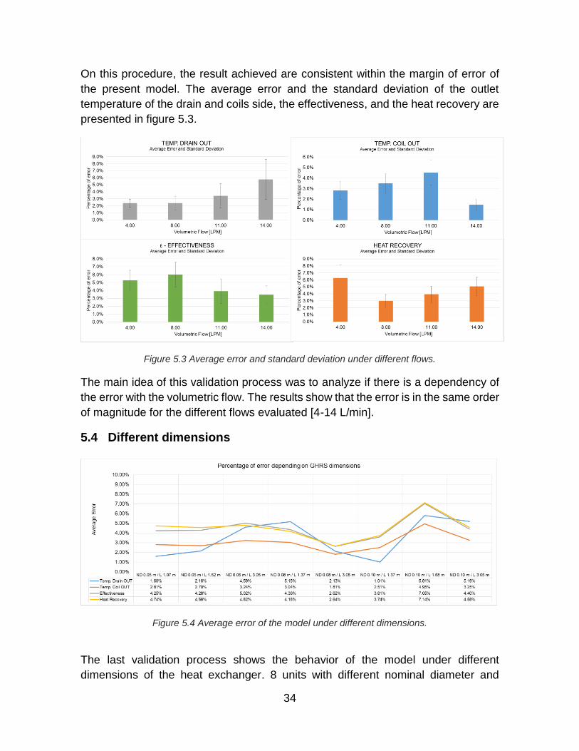
On this procedure, the result achieved are consistent within the margin of error of

the present model. The average error and the standard deviation of the outlet

temperature of the drain and coils side, the effectiveness, and the heat recovery are

presented in figure 5.3.

Figure 5.3 Average error and standard deviation under different flows.

The main idea of this validation process was to analyze if there is a dependency of

the error with the volumetric flow. The results show that the error is in the same order

of magnitude for the different flows evaluated [4-14 L/min].

5.4 Different dimensions

Figure 5.4 Average error of the model under different dimensions.

The last validation process shows the behavior of the model under different

dimensions of the heat exchanger. 8 units with different nominal diameter and

35

different lengths were the subject of study under different flow conditions and the

average error was calculated for 4 variables (Outlet drain Temperature, Outlet coil

Temperature, Effectiveness, and Heat Recovery).

The figure 5.4 shows that the error for the 4 evaluated variables is at the same order

of magnitude alongside the different dimensions evaluated. With this process, the

model shows that its results are stable for the dimension evaluated that were:

nominal diameter of 0.05-0.10 [m], length 0.91-3.05 [m] and 4-6 coils.

36

6 MODEL SIMULATIONS

In the previous chapter, the heat transfer model proposed was validated. In this

chapter, the effectiveness dependency for variables such as the dimensions,

number of coils and analyzes about the outlet temperature of the results of the model

are explained.

For this model, the code was developed in MATLAB with a Graphic User Interface

(GUI) following the process described in chapter 4.

Figure 6.1 Screenshot from the MATLAB GUI of the model.

Figure 6.1 shows one of the screenshots of the MATLAB GUI. This figure is the main

program in which general calculation for a heat exchanger can be done. In this

interface, the other calculations such as the economic analyses can be reached. For

these additional screenshots, refer to APPENDIX E.

With this model, different simulation can be run. Table 6-1 shows the results for

several heat exchangers with different diameters and different lengths. This test

used standard conditions of 9 [L/min], 36 °C as inlet temperature on the drain side

and 8°C at the coil side. The dimensions evaluated were for a heat exchanger with

4 coils with a nominal diameter of 0.05, 0.08 and 0.10 [m] and lengths in the range

of 0.91-3.05 [m].

A complete table of results can be found in APPENDIX C. With this full table of

results, some graphics were created to analyze some of the performance trends of

the greywater heat exchangers.

37

GE

OM

ET

RY

Le

ng

th [

m]

Eff

ecti

ven

ess

q [

kW

]

Td

rain

_o

ut

[°C

]

Tc

oil

_o

ut

[°C

]

NT

U

UA

[W

/K]

ReD

rain

ReC

oil

Reg

imeC

oil

R1 [

K/W

]

R2 [

K/W

]

R3 [

K/W

]

R4 [

K/W

]

R5 [

K/W

]

Rto

tal

[K/W

]

Cco

il

Cd

rain

No

min

al

Dia

me

ter

= 0

.05

[m

]

Nu

mb

er

of

co

ils

= 4

0.91 31.06% 5.43 27.30 16.65 0.450 281.0 4933.9 4876.6 Laminar 1.53E-03 3.36E-05 2.59E-04 3.27E-05 1.70E-03 3.56E-03 627.46 624.40

1.07 34.63% 6.06 26.30 17.65 0.529 330.5 4883.3 4943.9 Laminar 1.31E-03 2.85E-05 2.20E-04 2.78E-05 1.44E-03 3.03E-03 627.36 624.50

1.22 37.66% 6.59 25.45 18.50 0.603 376.9 4840.4 5001.2 Laminar 1.16E-03 2.50E-05 1.93E-04 2.44E-05 1.25E-03 2.65E-03 627.29 624.59

1.37 40.42% 7.07 24.68 19.27 0.678 423.3 4801.6 5053.6 Laminar 1.04E-03 2.23E-05 1.72E-04 2.17E-05 1.11E-03 2.36E-03 627.22 624.67

1.52 42.95% 7.51 23.97 19.98 0.752 469.6 4766.1 5101.8 Laminar 9.41E-04 2.01E-05 1.55E-04 1.96E-05 9.94E-04 2.13E-03 627.16 624.74

1.68 45.41% 7.95 23.28 20.67 0.831 519.0 4731.5 5148.9 Laminar 8.56E-04 1.82E-05 1.40E-04 1.77E-05 8.95E-04 1.93E-03 627.11 624.81

1.83 47.54% 8.32 22.69 21.26 0.905 565.3 4701.8 5189.7 Laminar 7.89E-04 1.67E-05 1.29E-04 1.62E-05 8.18E-04 1.77E-03 627.06 624.87

2.13 51.33% 8.98 21.63 22.32 1.053 657.9 4649.1 5262.7 Laminar 6.84E-04 1.43E-05 1.11E-04 1.40E-05 6.97E-04 1.52E-03 626.99 624.97

2.44 54.70% 9.57 20.68 23.27 1.205 753.4 4602.2 5328.1 Laminar 6.01E-04 1.25E-05 9.66E-05 1.22E-05 6.05E-04 1.33E-03 626.92 625.06

2.74 57.55% 10.07 19.89 24.07 1.353 845.8 4562.9 5383.4 Laminar 5.39E-04 1.11E-05 8.61E-05 1.08E-05 5.35E-04 1.18E-03 626.86 625.13

3.05 60.13% 10.53 19.16 24.79 1.505 941.1 4527.2 5433.9 Laminar 4.87E-04 1.00E-05 7.73E-05 9.75E-06 4.78E-04 1.06E-03 626.81 625.20

No

min

al

Dia

me

ter

= 0

.08

[m

]

Nu

mb

er

of

co

ils

= 4

0.91 38.36% 6.71 25.26 18.69 0.621 388.1 3019.2 5014.3 Laminar 1.14E-03 2.13E-05 1.67E-04 2.13E-05 1.23E-03 2.58E-03 627.27 624.61

1.07 42.25% 7.39 24.17 19.78 0.731 456.4 2984.9 5088.5 Laminar 9.75E-04 1.81E-05 1.42E-04 1.81E-05 1.04E-03 2.19E-03 627.18 624.72

1.22 45.48% 7.96 23.27 20.69 0.833 520.4 2956.6 5150.2 Laminar 8.61E-04 1.59E-05 1.24E-04 1.59E-05 9.04E-04 1.92E-03 627.11 624.81

1.37 48.36% 8.46 22.46 21.50 0.935 584.3 2931.5 5205.6 Laminar 7.72E-04 1.41E-05 1.11E-04 1.41E-05 8.01E-04 1.71E-03 627.05 624.89

1.52 50.95% 8.92 21.73 22.22 1.037 648.2 2908.9 5255.5 Laminar 7.00E-04 1.27E-05 9.97E-05 1.27E-05 7.18E-04 1.54E-03 626.99 624.96

1.68 53.45% 9.35 21.04 22.92 1.146 716.3 2887.3 5303.7 Laminar 6.37E-04 1.15E-05 9.02E-05 1.15E-05 6.46E-04 1.40E-03 626.94 625.03

1.83 55.56% 9.72 20.44 23.51 1.248 780.1 2868.9 5344.8 Laminar 5.87E-04 1.06E-05 8.28E-05 1.06E-05 5.91E-04 1.28E-03 626.90 625.08

2.13 59.26% 10.37 19.41 24.55 1.452 907.6 2837.0 5416.9 Laminar 5.09E-04 9.09E-06 7.12E-05 9.09E-06 5.04E-04 1.10E-03 626.83 625.18

2.44 62.48% 10.94 18.51 25.45 1.662 1039.1 2809.3 5480.0 Laminar 4.47E-04 7.94E-06 6.21E-05 7.94E-06 4.37E-04 9.62E-04 626.77 625.26

2.74 65.15% 11.41 17.76 26.20 1.865 1166.3 2786.5 5532.4 Laminar 4.01E-04 7.07E-06 5.53E-05 7.07E-06 3.87E-04 8.57E-04 626.72 625.33

3.05 67.53% 11.82 17.09 26.87 2.075 1297.7 2766.1 5579.4 Laminar 3.62E-04 6.35E-06 4.97E-05 6.35E-06 3.46E-04 7.71E-04 626.68 625.38

No

min

al

Dia

me

ter

= 0

.10

[m

]

Nu

mb

er

of

co

ils

= 4

0.91 42.10% 7.36 24.21 19.74 0.726 453.6 2389.0 5085.5 Laminar 9.88E-04 1.71E-05 1.35E-04 1.73E-05 1.05E-03 2.20E-03 627.18 624.72

1.07 46.09% 8.06 23.10 20.86 0.854 533.3 2361.1 5161.8 Laminar 8.48E-04 1.45E-05 1.14E-04 1.47E-05 8.84E-04 1.88E-03 627.09 624.83

1.22 49.35% 8.64 22.18 21.77 0.973 608.0 2338.3 5224.6 Laminar 7.49E-04 1.28E-05 1.00E-04 1.29E-05 7.70E-04 1.64E-03 627.03 624.92

1.37 52.24% 9.14 21.37 22.58 1.092 682.6 2318.1 5280.5 Laminar 6.71E-04 1.14E-05 8.94E-05 1.15E-05 6.82E-04 1.47E-03 626.97 625.00

1.52 54.82% 9.59 20.65 23.30 1.211 757.1 2300.3 5330.4 Laminar 6.08E-04 1.02E-05 8.05E-05 1.03E-05 6.11E-04 1.32E-03 626.92 625.06

1.68 57.28% 10.03 19.96 23.99 1.338 836.6 2283.3 5378.2 Laminar 5.53E-04 9.27E-06 7.29E-05 9.35E-06 5.50E-04 1.20E-03 626.87 625.13

1.83 59.35% 10.39 19.38 24.57 1.457 911.0 2269.0 5418.6 Laminar 5.10E-04 8.51E-06 6.69E-05 8.59E-06 5.03E-04 1.10E-03 626.83 625.18

2.13 62.94% 11.02 18.38 25.58 1.695 1059.7 2244.3 5489.0 Laminar 4.42E-04 7.31E-06 5.75E-05 7.38E-06 4.29E-04 9.44E-04 626.76 625.27

2.44 66.04% 11.56 17.51 26.45 1.940 1213.3 2223.1 5549.9 Laminar 3.89E-04 6.38E-06 5.02E-05 6.44E-06 3.73E-04 8.24E-04 626.71 625.35

2.74 68.57% 12.01 16.80 27.16 2.177 1361.7 2205.7 5600.1 Laminar 3.48E-04 5.68E-06 4.47E-05 5.73E-06 3.30E-04 7.34E-04 626.66 625.41

3.05 70.82% 12.40 16.17 27.79 2.422 1515.0 2190.4 5644.7 Laminar 3.14E-04 5.10E-06 4.01E-05 5.15E-06 2.95E-04 6.60E-04 626.62 625.46

Table 6-1 Simulation results for different GHE with different dimensions.

6.1 Dimensions

Figure 6.2 shows the change in effectiveness for different dimensions. One of the

first conclusions that can be stated is that bigger diameters performed better than

small ones. With the length, a similar phenomenon is depicted. A longer heat

exchanger can transfer more heat than short ones. For this reason, long units

performed with higher effectiveness than short heat exchangers.

38

Figure 6.2 Effectiveness dependency on GHE dimensions.

6.2 Number of coils

A reference unit of 0.05 m of nominal diameter was used to evaluate the impact of

numbers of coils. Figure 6.3 shows that higher number of coils will perform worse

than with less number of coils. The main reason why it is important to have several

numbers of coils is that the pressure drop will be lower for those cases (Guo et al.

2001).

Figure 6.3 Effectiveness performance for different number of coils.

39

6.3 Outlet temperatures

The outlet temperatures were evaluated for a reference unit with a nominal diameter

of 0.08 m and 4 coils. As it is expected, shorter unit will perform worse than longer

units. The temperatures achieve for short units are less than the ones achieve with

longer exchangers as shown in figure 6.4.

Figure 6.4 Simulation for outlet temperatures.

40

7 POTENTIAL OF IMPLEMENTATION

Directives from the European Union have pointed out the importance of increasing

the energy efficiency in buildings. In addition, Sweden has established a law in which

all new buildings should fulfill the regulation of nearly zero energy buildings (NZEB)

from 2020, implemented according to the EU Energy performance of buildings

directive (Wallin & Claesson 2014). GHRS raise in importance in order to achieve

this goal.

In the real world, what makes a technology or idea succeed between others is how

economically feasible it is. A study in Poland (Słyś & Kordana 2014) analyzed the

economic aspect of the GHRS for household consumers. As the first conclusion, the

potential of recovering the investment is directly proportional to the amount of hot

water used. Logically, it would be the total water consumption of the whole

household which determined how economically feasible the concept is.

The findings of this study state that the discount payback period can range from

almost 2.5 years to less than 10 years depending directly on the shower duration

and the volume of hot water used (Słyś & Kordana 2014).

On this chapter, some of the characteristics of the variables that influence the

implementation of GHRS are the subject of study.

7.1 Water Usage

One of the most important variables for the economic feasibility of GHRS is the water

usage. The main concern is that not everyone use the same amount of water and

neither take the same time during showers. The variability of water usage is

tremendous and several factors influence them (Opitz et al. 1999). It is important to

estimate a pattern of water usage during shower time. Studies (Blokker et al. 2010;

Athuraliya et al. 2012; Lallana et al. 2001) have acquired theoretical and empirical

data to simulate these patterns.

Firstly, countries use water for different purposes with different applications. This can

be easily explained with table 7-1. A comparison in the water pattern in percentage

depending on the application is done between England, Finland, and Switzerland.

Finland uses only 14% of their household water for toilet flushing, different from

England and Switzerland that use a 33%. The situation changes drastically with a

higher use of washing machine and dishwashing in Finland than in the other

countries.

41

HOUSEHOLD USES ENGLAND

AND WALES (%)

FINLAND (%) SWITZERLAND

(%)

Toilet flushing 33 14 33

Bathing and showering 20 29 32

Washing machines and dishwashing

14 30 16

Drinking and cooking 3 4 3

Miscellaneous 27 21 14

External use 3 2 2

Table 7-1 Patterns of water use by households in England and Wales, Finland and Switzerland.

Source: ((UK Department of the Environment, 1997; Etelämäki, 1999) cited by Lallana et al. 2001)

For bathing and showering, England uses a 20% of the water, while Finland and

Switzerland use a 29% and 32% respectively. These facts show a clear difference

between different countries on how the water usage share differs from one to

another. Specific information on the water consumption with this differentiation of

applications for Sweden was not found and a simulated profile was required.

Blokker et al. (2010) proposed a water demand end-use model that predicts water

demand for small time scale at a residential level. The model is based on information

from statistical data of users and end-uses.

The model proposes different distribution for different end-uses. Specifically talking

about most important concerning greywater for GHE, the model proposes the next

distributions for the Netherlands.

APPLICATION Frequency

[1/day] Duration Intensity [L/s]

End Use Type Avg, Distribution Avg Distribution Avg. Distribution

Dishwasher Brand and

type 0.3 Poisson

Specific dishwashing pattern ( 4 cycles of water entering, total 84 seconds,

0.167 L/ sec=14 L )

Washing Machine

Brand and type

0.3 Poisson Specific washing pattern ( 4 cycles of water entering, total 5 minutes, 0.167

L/ sec=50 L )

Shower

Normal

0.7 Binominal 8.5 min

x^2 Distribution

0.142 N.A.

(Fixed) Water Saving

0.123

Table 7-2 Frequency, Duration, and Intensity for Several Types and Subtypes of End-Uses in the Netherlands.

Source: (Blokker et al. 2010)

42

The shower duration has a strong dependency with the age of the inhabitants.

Children and teenagers take longer showers than adults. Additionally, the water

intensity for shower depends on the type of water heater (Blokker et al. 2010).

Another study was presented by Athuraliya et al. (2012) where they performed a

major research to measure the residential water usage at the end-level for the city

of Melbourne, Australia. 337 households were evaluated for two weeks of the winter

2010 and two of summer 2012.

The result shows a major use of water during the summer season, but for the

simplicity of the present work, only the average between seasons was taken into

account. Figure 7.1 shows the different Poisson distributions of water usage. The

shower time simulated shows a distribution in the top left graphic with an average

value of 6.5 minutes per person. The flow distribution is depicted in the top right

graphic with an average value of 7.29 L/min (0.1215 L/s) during showering. The total

water usage per shower is shown in the bottom graphic where the mean value is

47.17 Liters per person. The total water usage for 80% of the cases is below 70

Liters.

Figure 7.1 Water usage pattern during shower. Source: (Athuraliya et al. 2012)

The present distribution will be used further to analyses the economic feasibility of

GHE if applied to n-number of household with this distributed pattern of showering.

The condition presented on Athuraliya et al. (2012) distribution is a worse scenario

than the distribution proposed by Blokker et al. (2010) and this is the main reason of

selecting this pattern to simulate the consumption of Sweden.

43

7.2 Persons per Household

The number of persons per household is another important variable in order to

understand the potential of GHRS in residential households. It is easily recognizable

that the more people living in the same household, the higher water consumption will

be and the more economically feasible the GHRS will be.

Table 7-3 Persons per Households in Sweden 2015.

Source: (SCB-Sweden 2016)

Figure 7.2 shows the distribution of persons per households and households with n-

persons. These results can be found in the table 7-3 where it is clearly stated that

most people live in 2-persons households with 30.87%. The most common type of

household is the single person one with 37.39%. The average number of persons

living per household in Sweden is 2.21 (SCB-Sweden 2016). The full statistical

distribution of households can be found in Table D-1 in APPENDIX D.

Figure 7.2 Distribution of households in Sweden 2015. Source: (SCB-Sweden 2016)

These numbers are important to understand that the implementation of GHRS is

related as well to the persons living in the different households. This number varies

with several conditions and it is also different from country to country in Europe, as

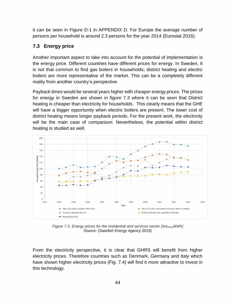
44

it can be seen in Figure D-1 in APPENDIX D. For Europe the average number of

persons per household is around 2.3 persons for the year 2014 (Eurostat 2016).

7.3 Energy price

Another important aspect to take into account for the potential of implementation is

the energy price. Different countries have different prices for energy. In Sweden, It

is not that common to find gas boilers in households; district heating and electric

boilers are more representative of the market. This can be a completely different

reality from another country’s perspective.

Payback times would be several years higher with cheaper energy prices. The prices

for energy in Sweden are shown in figure 7.3 where it can be seen that District

heating is cheaper than electricity for households. This clearly means that the GHE

will have a bigger opportunity when electric boilers are present. The lower cost of

district heating means longer payback periods. For the present work, the electricity

will be the main case of comparison. Nevertheless, the potential within district

heating is studied as well.

Figure 7.3. Energy prices for the residential and services sector [öre2013/kWh] Source: (Swedish Energy Agency 2015)

From the electricity perspective, it is clear that GHRS will benefit from higher

electricity prices. Therefore countries such as Denmark, Germany and Italy which

have shown higher electricity prices (Fig. 7.4) will find it more attractive to invest in

this technology.

45

Figure 7.4 Electricity price for household consumers 2015 [€/kWh] Source: (Eurostat 2016) (Online data code: nrg_pc_204)

7.4 GHRS Unit dimensions & Investment

In the market, several different GHRS units can be found with different sizes, number

of coils, diameters and effectiveness values, as well that with a diverse price range.

The configuration of the units plays an important role. It is different to analyze the

potential of implementation in a single household than in a multi-dwelling one. All of

these characteristics are key aspects to develop an economic analysis, due that

different models will generate diverse results.

The cost of the unit varies on its dimensions. Bigger units with a better performance

are more expensive than smaller ones with lower performance in comparison. In

addition, the installation cost varies from country to country and influence directly the

investment cost. For the cheaper units, the installation cost could account for almost

50% of the total investment cost according to the cost proposed by a manufacturer

(ReneWABILITY 2016). These variables influence directly the economic potential of

the technology.

46

8 ECONOMIC ANALYSIS

As seen in the previous chapter, several variables influence the performance and

economic feasibility for the implementation of GHRS. This section will join all these

variables in order to understand an economic analysis for this technology. The work

of Słyś & Kordana (2014) presents a calculation model to estimate the financial

efficiency of projects with GHRS. This model was used as based for the present

work and additionally, a Monte Carlo simulation was performed in order to estimate

the potential for an n-number of households using one exchanger per household.

The main methodology consists of a reference case without a GHRS unit and a

further comparison with the savings produce due the higher temperature of the

incoming water preheated from the coil side. The main objective was to obtain the

Discounted Payback Period (DPP) for different units on several operational

conditions.

It is important to remark that the result in this section should not be taken as given,

but just as results to explore the potential of the technology from an economic point

of view due some of the assumptions made through the simulation.

8.1 Reference Case

The first step to describe the energy cost for the reference case begins with the

equation 8.1 (Słyś & Kordana 2014) which define Vref_cold as the flow of cold water

for the mixture of shower. Where Vshower is the water flow of the shower [m^3/s] (Refer

to section 7.1); Twmix is the temperature of the shower and it is assumed to be 38°C

(301 K) for the present work; Twhot the temperature of hot water 60°C (333 K); Twcold

the temperature of the cold water 8°C (281 K) or the inlet temperature of the coil

side; with Cp as the specific heat and ρ as the density of the fluid.

��𝑟𝑒𝑓_𝑐𝑜𝑙𝑑 = ��𝑠ℎ𝑜𝑤𝑒𝑟 ∗ (

𝐶𝑝0 ∗ 𝜌0 ∗ (𝑇𝑤𝑚𝑖𝑥 − 𝑇𝑤𝑐𝑜𝑙𝑑)

𝐶𝑝0 ∗ 𝜌0 ∗ (𝑇𝑤ℎ𝑜𝑡 − 𝑇𝑤𝑚𝑖𝑥) + 𝐶𝑝0 ∗ 𝜌0 ∗ (𝑇𝑤𝑐𝑜𝑙𝑑 − 𝑇𝑤𝑚𝑖𝑥)) (8.1)

Secondly, the energy required for one year to heat up the cold water up to the hot

water temperature (Eref) is computed from equation 8.2 where: Days is the numbers

of days of the computation (yearly base, therefore, it is 365); Pers is the number of

inhabitants in the household (Refer to section 7.2); tshower is the duration of the

shower [s] (Refer to section 7.1); ηboiler is the efficiency of the boiler.

𝐸𝑟𝑒𝑓 = 𝐷𝑎𝑦𝑠 ∗ 𝑃𝑒𝑟𝑠 ∗ 𝑡𝑠ℎ𝑜𝑤𝑒𝑟 ∗ 𝑉𝑟𝑒𝑓_𝑐𝑜𝑙𝑑 ∗ 𝐶𝑝0 ∗ 𝜌0 ∗𝑇𝑤ℎ − 𝑇𝑤𝑐

𝜂𝑏𝑜𝑖𝑙𝑒𝑟 ∗ 3.6𝐸6 (8.2)

47

Finally, the total cost of the electricity for one year is calculated using equation 8.3

where: PricekWh is the price of electricity per kWh (1.7 SEK2014/kWh). For district

heating, the average cost is 0.74 SEK2014 (Swedish Energy Agency 2015).

𝑃𝑟𝑖𝑐𝑒𝑟𝑒𝑓 = 𝐸𝑟𝑒𝑓 ∗ 𝑃𝑟𝑖𝑐𝑒𝑘𝑊ℎ (8.3)

8.2 GHRS Case

The cost of energy using GHRS is computed in the same way as the reference case.

The difference is that the cold water temperature is now the preheated water coming

from the outlet of the GHRS which is defined as Tcoil_out. In equation 8.4.

𝑉𝐺𝐻𝑅𝑆 =

𝑉𝑠ℎ𝑜𝑤𝑒𝑟 ∗ (𝐶𝑝𝑐𝑜𝑖𝑙 ∗ 𝜌𝑐𝑜𝑖𝑙) ∗ (𝑇𝑤𝑚𝑖𝑥 − 𝑇𝑐𝑜𝑖𝑙𝑜𝑢𝑡)

((𝐶𝑝𝑐𝑜𝑖𝑙 ∗ 𝜌𝑐𝑜𝑖𝑙) ∗ (𝑇𝑤ℎ𝑜𝑡 − 𝑇𝑤𝑚𝑖𝑥)) + ((𝐶𝑝𝑐𝑜𝑖𝑙 ∗ 𝜌𝑐𝑜𝑖𝑙) ∗ (𝑇𝑤𝑚𝑖𝑥 − 𝑇𝑐𝑜𝑖𝑙𝑜𝑢𝑡)) (8.4)

In the same way, with the GHE, the water does not have to heat up from the initial

temperature. It is preheated on the GHE and it will require less energy to achieve

the required temperature.

𝐸𝐺𝐻𝑅𝑆 = 𝐷𝑎𝑦𝑠 ∗ 𝑃𝑒𝑟𝑠 ∗ 𝑡𝑠ℎ𝑜𝑤𝑒𝑟 ∗ 𝑉𝐺𝐻𝑅𝑆 ∗ 𝐶𝑝𝑐𝑜𝑖𝑙 ∗ 𝜌𝑐𝑜𝑖𝑙 ∗

𝑇𝑤ℎ𝑜𝑡 − 𝑇𝑐𝑜𝑖𝑙𝑜𝑢𝑡𝜂𝑏𝑜𝑖𝑙𝑒𝑟 ∗ 3.6𝐸6

(8.5)

The operational cost is calculated, obtaining lower cost than the reference case

without GHRS.

𝑃𝑟𝑖𝑐𝑒𝐺𝐻𝑅𝑆 = 𝐸𝐺𝐻𝑅𝑆 ∗ 𝑃𝑟𝑖𝑐𝑒𝑘𝑊ℎ (8.6)

𝑆𝑎𝑣𝑖𝑛𝑔𝑠𝑝𝑒𝑟𝑖𝑜𝑑 = 𝑃𝑟𝑖𝑐𝑒𝑟𝑒𝑓 − 𝑃𝑟𝑖𝑐𝑒𝐺𝐻𝑅𝑆 (8.7)

The saving on the period of the first year is defined by equation 8.7.

8.3 Net Present Value

To evaluate the economic benefits of GHE the Net Present Value must be

considered due the fact that money has different value through time. Money from

one specific year has a net value different than the same amount of money in another

period of time.

48

On this step, the net present savings during the lifetime of the device that is 50 years

according to one manufacturer (ReneWABILITY 2016) but for the computation, only

20 years are taking into account. The internal rate of return (r) is assumed to be 8%.

𝑁𝑃𝑉𝑟𝑒𝑓 = 𝑃𝑟𝑖𝑐𝑒𝑟𝑒𝑓 ∗ (

1 − (1 + 𝑟)−𝑡

𝑟)

𝑁𝑃𝑉𝐺𝐻𝑅𝑆 = 𝑃𝑟𝑖𝑐𝑒𝐺𝐻𝑅𝑆 ∗ (1 − (1 + 𝑟)−𝑡

𝑟)

(8.8)

𝑆𝑎𝑣𝑖𝑛𝑔𝑠𝑆𝐸𝐾 = 𝑁𝑃𝑉𝐺𝐻𝑅𝑆 −𝑁𝑃𝑉𝑟𝑒𝑓 (8.9)

8.4 Discounted Payback Period

In economics, there is an important variable known as the Discounted Payback

Period (DPP) which gives the number of years to achieve the breakeven point of the

investment. It is computed using equation 8.10 where Invest is the initial investment

cost, Savingsperiod is the saving on a period of one year and r is the internal return

rate.

𝐷𝑃𝑃 =

𝑙𝑛(1

1 − (𝐼𝑛𝑣𝑒𝑠𝑡 ∗𝑟

𝑆𝑎𝑣𝑖𝑛𝑔𝑠𝑝𝑒𝑟𝑖𝑜𝑑))

𝑙𝑛(1 + 𝑟)

(8.10)

Due the complexity of water usage for different household and the numerous

variables involve the analysis of GHRS, giving a single result is a challenging

situation. Variables such as shower time, shower flow, investments, dimension,

effectiveness and others must be taken into account.

As seen in figure 8.1, the DPP is extremely sensitive to many factors. The proper

dimensioning of the unit is fundamental to make it economically feasible. This

computation was based on the retail prices available at the website of the

manufacturer (ReneWABILITY 2016) and an approximate installation fee. In figure

8.1(a), a unit of 0.05 of nominal diameter and 1.22 m of length for 4 inhabitants per

household, the payback time is below 10 years for all the possible configuration of

flow and shower time proposed. On the other hand, for only 2 inhabitants per

household it is still profitable and under 5 years of payback time for water intensive

49

users. On the low usage region (Short shower time and low water intensity), it is

impossible to reach a break-even point.1

This trend can be seen more easily in figure 8.1(b) whereas a product of the lower

prices of district heating; the region that is unable to reach the breakeven point is

bigger.

Figure 8.1 DPP Analysis for two GHRS under different condition of shower time and flow.

1 The results should not be taking as given for a market analysis. The only purpose is to give

a rough estimation of the potential implementation of GHRS from the economic point of view.

DPP with electricity price.

b) DPP with electricity price.

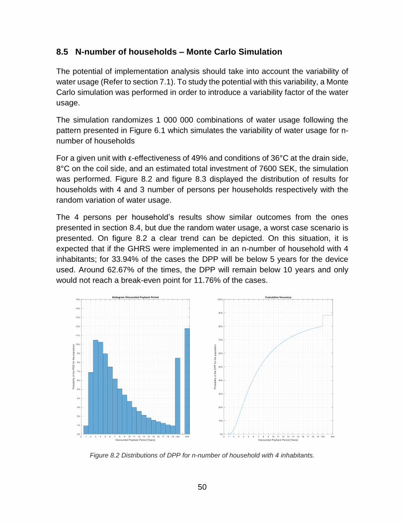
50

8.5 N-number of households – Monte Carlo Simulation

The potential of implementation analysis should take into account the variability of

water usage (Refer to section 7.1). To study the potential with this variability, a Monte

Carlo simulation was performed in order to introduce a variability factor of the water

usage.

The simulation randomizes 1 000 000 combinations of water usage following the

pattern presented in Figure 6.1 which simulates the variability of water usage for n-

number of households

For a given unit with ε-effectiveness of 49% and conditions of 36°C at the drain side,

8°C on the coil side, and an estimated total investment of 7600 SEK, the simulation

was performed. Figure 8.2 and figure 8.3 displayed the distribution of results for

households with 4 and 3 number of persons per households respectively with the

random variation of water usage.

The 4 persons per household’s results show similar outcomes from the ones

presented in section 8.4, but due the random water usage, a worst case scenario is

presented. On figure 8.2 a clear trend can be depicted. On this situation, it is

expected that if the GHRS were implemented in an n-number of household with 4

inhabitants; for 33.94% of the cases the DPP will be below 5 years for the device

used. Around 62.67% of the times, the DPP will remain below 10 years and only

would not reach a break-even point for 11.76% of the cases.

Figure 8.2 Distributions of DPP for n-number of household with 4 inhabitants.

51

For the figure 8.3 that correspond for 3 persons per household, it is expected to

decrease the values achieved. Even though the results display a good opportunity

for implementation. On this case, for 19.13% of the cases, the DPP will be below 5

years and 46.34% below 10. It would not reach a break-even point for 21.48% of the

occasions. 2

Figure 8.3 Distributions of DPP for n-number of household with 3 inhabitants.

8.6 Emission savings

The allocation of emissions that comes from the electricity production of the country

can be seen as emission savings (Eq. 8.11).

𝑆𝑎𝑣𝑖𝑛𝑔𝑠𝑒𝑚𝑖𝑠𝑠𝑖𝑜𝑛𝑠 = 𝑆𝑎𝑣𝑖𝑛𝑔𝑠𝑘𝑊ℎ ∗ 𝐶𝑂2𝑘𝑊ℎ (8.11)

The energy saved by GHRS, which can range from 30-70% of the energy required

depending on the model used, is multiply by the gr CO2 emitted per kWh produced

from the electricity production graphic depending on the country (Figure 8.4).

District heating manages different concentrations of gr CO2 that can be computed

and give an estimation of the emissions saved.

2 The results should not be taking as given for a market analysis. The only purpose is to give a rough estimation of the potential implementation of GHRS from the economic point of view.

52

Figure 8.4 Graphic of gr CO2 per kWh in Europe - Electricity production 2009.

Source: (European Environment Agency 2011)

8.7 District Heating

In countries like Sweden, District heating accounts for 58% of the total energy use

in non-residential buildings and dwelling. Multi-dwelling buildings use half of this

share (29% of the total energy used) while the other half is shared between the non-

residential building and one/two-dwelling building with a 38% and 12% respectively

(Swedish Energy Agency 2015).

One big advantage of district heating over electricity is that it is available at a lower

price. The price of electricity per kWh is 1.7 SEK2014/kWh while for district heating is

0.74 SEK2014/kWh (Swedish Energy Agency 2015). Electricity price is around 229%

more expensive per kWh than district heating. This fact shows a challenge for

technologies like the GHRS which will face up harder scenarios to achieve a break-

even point from an economic point of view.

Nr

Co

ils

Nu

mb

er

of

pers

on

s

in h

ou

seh

old

Td

rain

IN

[°C

]

Tco

il I

N [

°C]

Insta

llati

on

Fee

[SE

K]

Sh

ow

er

Tim

e [

min

]

Vo

lum

etr

ic F

low

[L/m

in]

Inte

rest

rate

[%

]

Ele

ctr

icit

y P

ric

e

[SE

K/k

Wh

]

Dis

tric

t H

eati

ng

Pri

ce [

SE

K/k

Wh

]

4 4 36 8 3500 6.5 7.29 8 1.7 0.74

Table 8-1 Conditions for the comparison between electricity and district heating.

53

On this section, a comparison about the estimated discounted payback period (DPP)

for different greywater heat exchanger between electricity and district heating prices.

Table 8-1 present the conditions and parameters taken into account for the

comparison. Figure 8.5 shows the results achieved in this analysis.

Figure 8.5 Comparison between electricity and district.

For the order of magnitude, the usage of district heating as energy source increases

the DPP in an average of 4.67 times more than with electricity for the heat exchanger

evaluated. The average payback time for this conditions was around 5.8 years with

electricity and 27.1 years with district heating. This situation exposed the impact of

cheap energy for the implementation of the technology from an economic

perspective.

It is important to remark that the installation fee takes an important role for small

units and that is why bigger units amortize this cost better achieving lower payback

periods.

0.00

5.00

10.00

15.00

20.00

25.00

30.00

35.00

40.00

DP

P [

years

]

GHE Dimensions

Electricity District Heating

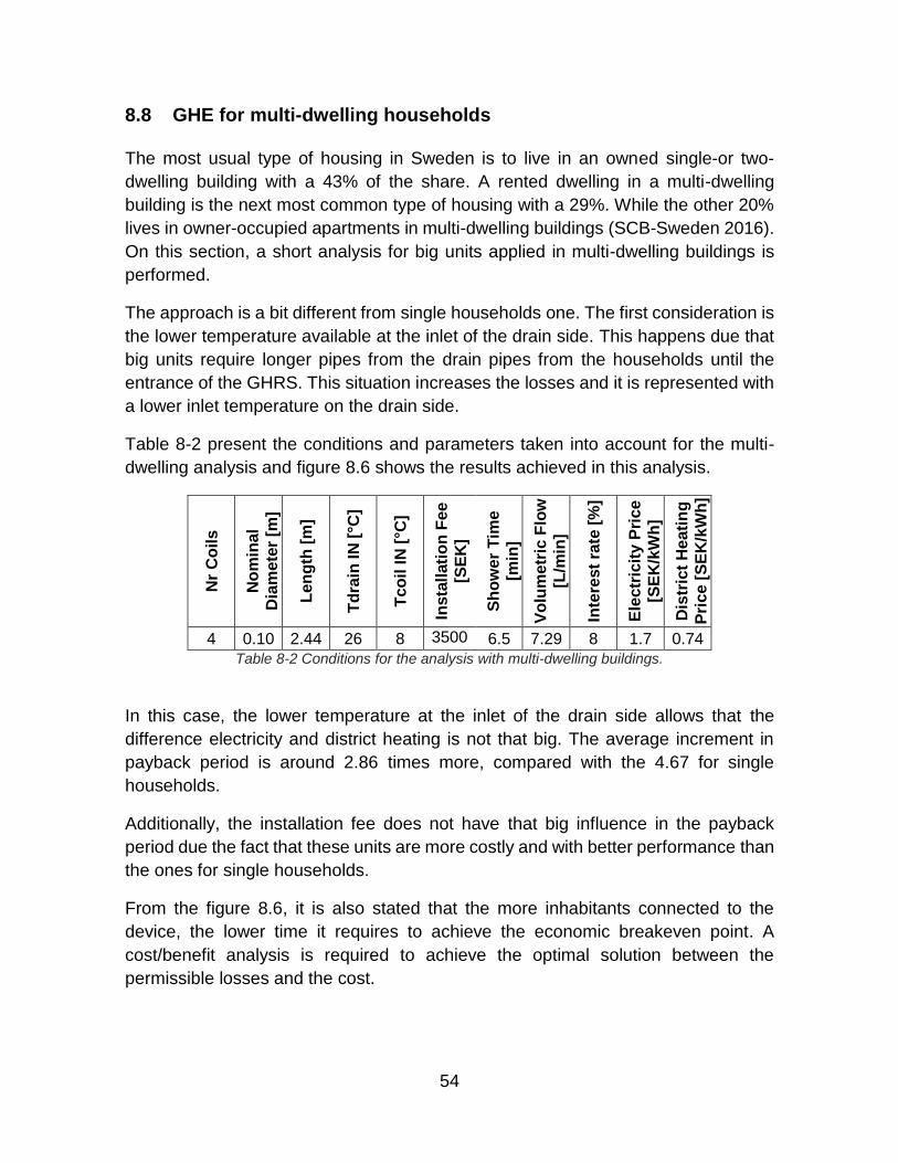
54

8.8 GHE for multi-dwelling households

The most usual type of housing in Sweden is to live in an owned single-or two-

dwelling building with a 43% of the share. A rented dwelling in a multi-dwelling

building is the next most common type of housing with a 29%. While the other 20%

lives in owner-occupied apartments in multi-dwelling buildings (SCB-Sweden 2016).

On this section, a short analysis for big units applied in multi-dwelling buildings is

performed.

The approach is a bit different from single households one. The first consideration is

the lower temperature available at the inlet of the drain side. This happens due that

big units require longer pipes from the drain pipes from the households until the

entrance of the GHRS. This situation increases the losses and it is represented with

a lower inlet temperature on the drain side.

Table 8-2 present the conditions and parameters taken into account for the multi-

dwelling analysis and figure 8.6 shows the results achieved in this analysis.

Nr

Co

ils

No

min

al

Dia

me

ter

[m]

Len

gth

[m

]

Td

rain

IN

[°C

]

Tco

il I

N [

°C]

Insta

llati

on

Fee

[SE

K]

Sh

ow

er

Tim

e

[min

]

Vo

lum

etr

ic F

low

[L/m

in]

Inte

rest

rate

[%

]

Ele

ctr

icit

y P

ric

e

[SE

K/k

Wh

]

Dis

tric

t H

eati

ng

Pri

ce [

SE

K/k

Wh

]

4 0.10 2.44 26 8 3500 6.5 7.29 8 1.7 0.74

Table 8-2 Conditions for the analysis with multi-dwelling buildings.

In this case, the lower temperature at the inlet of the drain side allows that the

difference electricity and district heating is not that big. The average increment in

payback period is around 2.86 times more, compared with the 4.67 for single

households.

Additionally, the installation fee does not have that big influence in the payback

period due the fact that these units are more costly and with better performance than

the ones for single households.

From the figure 8.6, it is also stated that the more inhabitants connected to the

device, the lower time it requires to achieve the economic breakeven point. A

cost/benefit analysis is required to achieve the optimal solution between the

permissible losses and the cost.

55

In general, units for multi-dwelling buildings achieve lower payback periods than

single households as it is also mentioned by one of the manufacturers

(ReneWABILITY 2016).

Figure 8.6 Comparison between electricity and district heating for multi-dwelling buildings.

0

2

4

6

8

10

12

14

161

0

12

14

16

18

20

22

24

26

28

30

DP

P [

years

]

Number of persons in the multi-dwelling

Electricity District Heating

56

9 CONCLUSIONS

The present study explored the different fluid mechanics characteristics of vertical

greywater heat exchangers. The first characteristic refers to the falling film effect

present in the drain side that maximizes the contact area between the fluid and the

inside area of the pipe. These conditions also minimize the thickness of the layer

turning the heat transfer mechanism more effective. Secondly, the helical coil

creates a secondary flow that increases the heat transfer coefficient significantly in

comparison with straight pipes and allows the transition to the turbulent regime to be

achieved at a higher Reynolds number than in straight pipes.

A theoretical heat transfer approach of the greywater heat exchanger was proposed

where a mathematical model was developed to simulate the performance of different

GHE. Different correlations available in the literature were evaluated to represent in

the most accurate way the performance of GHE. The model achieves a permissible

margin of error under different conditions of flow, temperatures, dimensions and

others. The heat recovery errors were below 6% for 75.93% of the times and below

10% for 92.59% of the times. The effectiveness of greywater heat exchanger

increase with its length and nominal diameter, being the influence of nominal

diameter bigger to achieve higher effectiveness values. The increase in the number

of coils decrease the effectiveness of the heat exchanger but it is beneficial for

decreasing the pressure drop on the device.

Greywater heat exchanger’s potential of implementation is influenced by several

variables. Water usage is one of the main variables and the variability of this aspect

has a deep implication on the potential of the technology. Not every inhabitant use

the same amount of water for different applications and there is a big fluctuation

between users. Additionally, the number of persons per household is important due

that the more people living in the same household, the higher water consumption will

be and the more economically feasible the GHRS will be. Another variable study in

the present work was the energy price. GHE will have a bigger opportunity when

electricity is used as the source of domestic hot water due its elevated priced

compared to district heating. The lower cost of district heating means longer payback

periods. The total cost of the device include the installation fee and this cost is

important for small units where it can account for 40-50% of the total price. With

lower effectiveness, small units present challenging situation to achieve break-even

points.

With the economic analysis performed, it can be stated that GHE present a higher

opportunity in a household with 3-4 inhabitant. This is not a rule due the variability

57

of water consumption patterns, but from a general point of view, it is more feasible

than for 1-2 inhabitants per household. Under average user consumptions, small

units can achieve a break-even point in around 5-6 years. District heating prices

increase this time by 4.7 times in comparison with electric boilers. For a multi-

dwelling household with big units, the technology is more feasible with a higher

number of households connected. Additionally, the technology has more potential

with big units even with lower energy prices. In the case of district heating, it only

represents an increment of 2.86 times compared to the 4.67 times of the single

households for one of the studies performed.

58

10 FUTURE RESEARCH

Empirical tests about the performance of greywater heat exchanger will validate the

characteristics studied about the technology. A deeper understanding of the

performance according to dimensions and flow conditions will generate better

information to quantify the benefits of GHRS. Additionally, long term effects can be

evaluated because until now, the analyses are taken as an assumption that the heat

exchanger will perform equally during its lifetime. The fouling effect can introduce

additional knowledge to understand the long-term performance of the devices.

This project studied the general concepts of fluid mechanics and heat transfer

involve in the technology. To go further, a CFD (Computational Fluid Dynamics)

analysis can be proposed in order to perform a deeper analysis on the different

devices and to work on optimizing the design to increase the efficiency and

performance of them.

The domestic hot water usage is one of the most important variables understanding

the potential of GHRS. During the development of the present work, a detailed study

concerning the water usage in Sweden was not found. There is information about

consumption per capita, total water usage but not about the patterns and usage in

different applications for households. This study would be interesting for the field and

with that information, a more accurate potential of implementation analysis can be

performed in addition to all the valuable knowledge for different fields around

conservation measures of water.

Most studies on the topic include baths and showers as the most important

application for GHRS. But greywater refers additionally to washbasins, kitchens,

washing machines, dishwashers and others. An additional study simulating these

conditions and impact of all greywater will enrich the discussion of the topic. The

waste water is also an opportunity to study in order to increase the efficiency in the

built environment.

As shown in the present work, several variables influence the economic feasibility of

GHRS. An extensive economic analysis with real-life cases could generate an

important database of the relation with the performance of the devices, the variability

of water usage and the economic performance. This information could generate

more accurate and meaningful conclusions about the economic potential as a cost

and effective solution.

59

11 REFERENCES

Athuraliya, A., Roberts, P. & Brown, A., 2012. Yarra Valley Future Water - Residential water use study volume 2. , 2(August), pp.1 – 46.

Austen, D.S. & Soliman, H.M., 1988. Laminar flow and heat transfer in helically coiled tubes with substantial pitch. Experimental Thermal and Fluid Science, 1(2), pp.183–194.

Blokker, E.J.M., Vreeburg, J.H.G. & Van Dijk, J.C., 2010. Simulating Residential Water Demand with a Stochastic End-Use Model. Journal of Water Resources Planning and Management, 136(January/February), pp.19–26.

Cengel, A. & Cimbala, J., 2006. Fluid mechanics: fundamentals and applications. International Edition, McGraw Hill Publication, pp.1–2023.

Collins, M., Decker, G. Van & Murray, J., 2013. Characteristic Effectiveness Curves for Falling Film Drain Water Heat Recovery Systems. HVAC&R Research, 19(January 2014), pp.649–662.

Collins, M.R., 2009. Effectiveness Testing of PowerPipe TM Drain Water Heat Recovery Systems. Solar Thermal Research Laboratory - University of Waterloo, p.156.

Dieckmann, J., 2012. Drain Water Heat Recovery Response. ASHRAE Journal, 54(1), p.13.

Elsayed, A.M., 2011. Heat transfer in helically coiled small diameter tubes for miniature cooling systems . , (September), p.333.

European Environment Agency, 2011. CO2 electricity per kWh. Available at: http://www.eea.europa.eu/data-and-maps/figures/co2-electricity-g-per-kwh/co2-per-electricity-kwh-fig-1_2010_qa.xls [Accessed April 2, 2016].

Eurostat, 2016. Europe Statistics. Available at: http://ec.europa.eu/eurostat [Accessed April 1, 2016].

Guo, L., Feng, Z. & Chen, X., 2001. An experimental investigation of the frictional pressure drop of steam–water two-phase flow in helical coils. International Journal of Heat and Mass Transfer, 44(14), pp.2601–2610.

Incropera, F.P. et al., 2007. Fundamentals of Heat and Mass Transfer 6th Editio. J. W. & Sons, ed.,

Janssen, L.A.M. & Hoogendoorn, C.J., 1978. Laminar convective heat transfer in helical coiled tubes. International Journal of Heat and Mass Transfer, 21(9), pp.1197–1206.

Jayakumar, J.S. et al., 2008. Experimental and CFD estimation of heat transfer in

60

helically coiled heat exchangers. chemical engineering research and design, 86(3), pp.221–232.

Korpar Malmström, S., 2015. En god natts sömn och återvunnen energi Modellering av avloppsvärmeväxling på ett stockholmshotell och spa Relax and sleep ( energy ) efficiently Modelling wastewater heat recovery in a. KTH.

Kozo, F. & Yoshiyuki, A., 1988. Laminar heat transfer in a helically coiled tube. International Journal of Heat and Mass Transfer, 31(2), pp.387–396.

Lallana, C. et al., 2001. Sustainable water use in Europe Part 2: Demand management,

Leidl, C.M. & David Lubitz, W., 2009. Comparing domestic water heating technologies. Technology in Society, 31(3), pp.244–256.

Lienhard IV, J.H. & Lienhard V, J.H., 1986. A heat transfer textbook Fourth Edi., Cambridge, Massachusetts, USA.: Phlogiston Press.

Manouchehri, R., 2015. Predicting Steady-State Performance of Falling-Film Drain Water Heat Recovery Systems from Rating Data. University of Waterloo.

McNabola, A. & Shields, K., 2013. Efficient drain water heat recovery in horizontal domestic shower drains. Energy and Buildings, 59, pp.44–49.

Naphon, P. & Wongwises, S., 2006. A review of flow and heat transfer characteristics in curved tubes. Renewable and Sustainable Energy Reviews, 10(5), pp.463–490.

Ni, L. et al., 2012. Feasibility study of a localized residential grey water energy-recovery system. Applied Thermal Engineering, 39, pp.53–62.

Opitz, E.M. et al., 1999. Residential End Uses of Water AWWA Research Foundation and American Water Works Association., ed., Denver, CO.

Prost, J.S., González, M.T. & Urbicain, M.J., 2006. Determination and correlation of heat transfer coefficients in a falling film evaporator. Journal of Food Engineering, 73(4), pp.320–326.

ReneWABILITY, 2016. Power-Pipe® Canadian & US Order. Available at: http://www.renewability.com/order_powerpipe_online.html [Accessed March 24, 2016].

Rogers, G.F.C. & Mayhew, Y.R., 1964. Heat transfer and pressure loss in helically coiled tubes with turbulent flow. International Journal of Heat and Mass Transfer, 7(11), pp.1207–1216.

SCB-Sweden, 2016. Number of persons and households and persons by households by region. Year 2011 - 2015. Population statistics. Available at: http://www.scb.se/be0101-en [Accessed April 20, 2016].

61

Słyś, D. & Kordana, S., 2014. Financial analysis of the implementation of a Drain Water Heat Recovery unit in residential housing. Energy and Buildings, 71, pp.1–11.

Swedish Energy Agency, 2015. Energy in Sweden 2015.

Vattenfall, 2015. Vattenfall e-learning. Available at: http://www.vattenfall.com/e-learning/ordlista.htm [Accessed February 15, 2016].

Wallin, J. & Claesson, J., 2014. Investigating the efficiency of a vertical inline drain water heat recovery heat exchanger in a system boosted with a heat pump. Energy and Buildings, 80, pp.7–16.

Wong, L.T., Mui, K.W. & Guan, Y., 2010. Shower water heat recovery in high-rise residential buildings of Hong Kong. Applied Energy, 87(2), pp.703–709.

Zaloum, C., Lafrance, M. & Gusdorf, J., 2007. Drain Water Heat Recovery Characterization and Modeling. Natural Resources Canada, pp.0–42.

62

APPENDIX A. Heat transfer model

START

GEOMETRIC INPUTSGHRS Diameters

LengthNumber of Coils

CASE INPUTSVolumetric Flow

Inlet Temperatures(Coil & Drain)

OTHERSIteration Output Temp

Constants (k_cooper, g,..)

FLUID THERMODYNAMIC PROPERTIES[Cp, µ, ρ, k, Pr] at average Temperature (T_in+T_out)/2 for both flows (Coil and Drain)

THERMAL CAPACITIESC_drain=m_dot_drain*Cp_drain

C_coil=m_dot_coil*Cp_coil*NrCoils

RESISTOR 1CONVECTION FILM

MINIMUM THERMAL CAPACITYC_min

VARIABLESReynolds

Heat Transfer Coefficient – Falling Film

CALCULATERESISTOR

Convection

RESISTOR 2CONDUCTION

DRAIN PIPE

NTU METHOD

Output Temperatures = Initial Output Temp

RESULT

CALCULATE RESISTOR

Conduction

RESISTOR 4CONDUCTION

COIL PIPE

RESISTOR 5CONVECTION

COIL

CALCULATE RESISTOR

Conduction

VARIABLESReynolds

Dean NumberNusselt Number

CALCULATEHeat Transfer

Coefficient

CALCULATERESISTOR

Convection

TOTAL THERMAL

RESISTANCEUA NTU

EffectivenessqOutput

TemperaturesIntial Output Temp = Output Temp

NO

YES

END

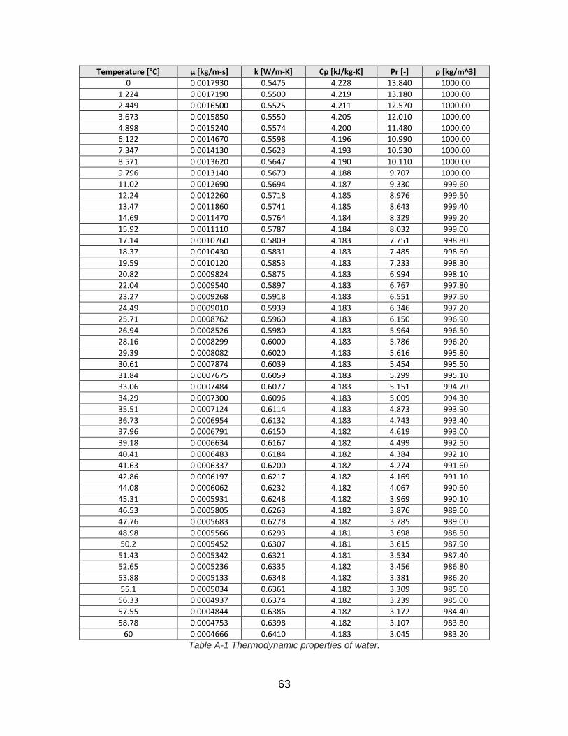
63

Temperature [°C] µ [kg/m-s] k [W/m-K] Cp [kJ/kg-K] Pr [-] ρ [kg/m^3]

0 0.0017930 0.5475 4.228 13.840 1000.00

1.224 0.0017190 0.5500 4.219 13.180 1000.00

2.449 0.0016500 0.5525 4.211 12.570 1000.00

3.673 0.0015850 0.5550 4.205 12.010 1000.00

4.898 0.0015240 0.5574 4.200 11.480 1000.00

6.122 0.0014670 0.5598 4.196 10.990 1000.00

7.347 0.0014130 0.5623 4.193 10.530 1000.00

8.571 0.0013620 0.5647 4.190 10.110 1000.00

9.796 0.0013140 0.5670 4.188 9.707 1000.00

11.02 0.0012690 0.5694 4.187 9.330 999.60

12.24 0.0012260 0.5718 4.185 8.976 999.50

13.47 0.0011860 0.5741 4.185 8.643 999.40

14.69 0.0011470 0.5764 4.184 8.329 999.20

15.92 0.0011110 0.5787 4.184 8.032 999.00

17.14 0.0010760 0.5809 4.183 7.751 998.80

18.37 0.0010430 0.5831 4.183 7.485 998.60

19.59 0.0010120 0.5853 4.183 7.233 998.30

20.82 0.0009824 0.5875 4.183 6.994 998.10

22.04 0.0009540 0.5897 4.183 6.767 997.80

23.27 0.0009268 0.5918 4.183 6.551 997.50

24.49 0.0009010 0.5939 4.183 6.346 997.20

25.71 0.0008762 0.5960 4.183 6.150 996.90

26.94 0.0008526 0.5980 4.183 5.964 996.50

28.16 0.0008299 0.6000 4.183 5.786 996.20

29.39 0.0008082 0.6020 4.183 5.616 995.80

30.61 0.0007874 0.6039 4.183 5.454 995.50

31.84 0.0007675 0.6059 4.183 5.299 995.10

33.06 0.0007484 0.6077 4.183 5.151 994.70

34.29 0.0007300 0.6096 4.183 5.009 994.30

35.51 0.0007124 0.6114 4.183 4.873 993.90

36.73 0.0006954 0.6132 4.183 4.743 993.40

37.96 0.0006791 0.6150 4.182 4.619 993.00

39.18 0.0006634 0.6167 4.182 4.499 992.50

40.41 0.0006483 0.6184 4.182 4.384 992.10

41.63 0.0006337 0.6200 4.182 4.274 991.60

42.86 0.0006197 0.6217 4.182 4.169 991.10

44.08 0.0006062 0.6232 4.182 4.067 990.60

45.31 0.0005931 0.6248 4.182 3.969 990.10

46.53 0.0005805 0.6263 4.182 3.876 989.60

47.76 0.0005683 0.6278 4.182 3.785 989.00

48.98 0.0005566 0.6293 4.181 3.698 988.50

50.2 0.0005452 0.6307 4.181 3.615 987.90

51.43 0.0005342 0.6321 4.181 3.534 987.40

52.65 0.0005236 0.6335 4.182 3.456 986.80

53.88 0.0005133 0.6348 4.182 3.381 986.20

55.1 0.0005034 0.6361 4.182 3.309 985.60

56.33 0.0004937 0.6374 4.182 3.239 985.00

57.55 0.0004844 0.6386 4.182 3.172 984.40

58.78 0.0004753 0.6398 4.182 3.107 983.80

60 0.0004666 0.6410 4.183 3.045 983.20

Table A-1 Thermodynamic properties of water.

64

Geometry R1 - CONVECTION

FALLING FILM R2 - CONDUCTION

DRAIN PIPE R3 - CONTACT

RESISTOR R4 - CONDUCTION

COIL PIPE R5 - CONVECTION

HELICAL COIL

TOTAL RESISTANCE

[K/W]

Length

[m] Resistor

[K/W] % of total resistance

Resistor [K/W]

% of total resistance

Resistor [K/W]

% of total resistanc

e

Resistor [K/W]

% of total resistance

Resistor [K/W]

% of total resistance

Nom

inal D

iam

ete

r =

0.0

5 m

Num

ber

of

Coils

= 4

0.91 1.531E-03 43.02% 3.357E-05 0.94% 2.591E-04 7.28% 3.267E-05 0.92% 1.702E-03 47.84% 3.5588E-03

1.07 1.312E-03 43.37% 2.855E-05 0.94% 2.204E-04 7.28% 2.778E-05 0.92% 1.437E-03 47.49% 3.0257E-03

1.22 1.158E-03 43.66% 2.504E-05 0.94% 1.933E-04 7.28% 2.437E-05 0.92% 1.252E-03 47.19% 2.6532E-03

1.37 1.038E-03 43.93% 2.230E-05 0.94% 1.721E-04 7.28% 2.170E-05 0.92% 1.109E-03 46.93% 2.3625E-03

1.52 9.405E-04 44.17% 2.010E-05 0.94% 1.551E-04 7.28% 1.956E-05 0.92% 9.941E-04 46.68% 2.1294E-03

1.68 8.556E-04 44.41% 1.818E-05 0.94% 1.403E-04 7.28% 1.770E-05 0.92% 8.948E-04 46.45% 1.9266E-03

1.83 7.891E-04 44.61% 1.669E-05 0.94% 1.288E-04 7.28% 1.624E-05 0.92% 8.179E-04 46.24% 1.7688E-03

2.13 6.837E-04 44.98% 1.434E-05 0.94% 1.107E-04 7.28% 1.396E-05 0.92% 6.973E-04 45.88% 1.5200E-03

2.44 6.014E-04 45.31% 1.252E-05 0.94% 9.663E-05 7.28% 1.218E-05 0.92% 6.046E-04 45.55% 1.3273E-03

2.74 5.390E-04 45.58% 1.115E-05 0.94% 8.605E-05 7.28% 1.085E-05 0.92% 5.353E-04 45.28% 1.1824E-03

3.05 4.870E-04 45.83% 1.001E-05 0.94% 7.731E-05 7.28% 9.747E-06 0.92% 4.785E-04 45.03% 1.0626E-03

Nom

inal D

iam

ete

r =

0.0

8 m

Num

ber

of

Coils

= 4

0.91 1.137E-03 44.13% 2.128E-05 0.83% 1.666E-04 6.47% 2.128E-05 0.83% 1.230E-03 47.75% 2.5764E-03

1.07 9.752E-04 44.51% 1.810E-05 0.83% 1.417E-04 6.47% 1.810E-05 0.83% 1.038E-03 47.37% 2.1909E-03

1.22 8.614E-04 44.83% 1.587E-05 0.83% 1.242E-04 6.47% 1.587E-05 0.83% 9.042E-04 47.06% 1.9216E-03

1.37 7.720E-04 45.11% 1.413E-05 0.83% 1.106E-04 6.46% 1.413E-05 0.83% 8.005E-04 46.78% 1.7114E-03

1.52 6.998E-04 45.36% 1.274E-05 0.83% 9.972E-05 6.46% 1.274E-05 0.83% 7.177E-04 46.52% 1.5427E-03

1.68 6.367E-04 45.61% 1.153E-05 0.83% 9.022E-05 6.46% 1.153E-05 0.83% 6.461E-04 46.28% 1.3961E-03

1.83 5.873E-04 45.81% 1.058E-05 0.83% 8.283E-05 6.46% 1.058E-05 0.83% 5.906E-04 46.08% 1.2819E-03

2.13 5.088E-04 46.17% 9.091E-06 0.83% 7.116E-05 6.46% 9.091E-06 0.83% 5.037E-04 45.72% 1.1019E-03

2.44 4.474E-04 46.49% 7.936E-06 0.82% 6.212E-05 6.46% 7.936E-06 0.82% 4.369E-04 45.40% 9.6234E-04

2.74 4.009E-04 46.75% 7.067E-06 0.82% 5.532E-05 6.45% 7.067E-06 0.82% 3.871E-04 45.15% 8.5739E-04

3.05 3.621E-04 46.99% 6.349E-06 0.82% 4.970E-05 6.45% 6.349E-06 0.82% 3.461E-04 44.92% 7.7061E-04

Nom

inal D

iam

ete

r =

0.1

m

Num

ber

of

Coils

= 4

0.91 9.878E-04 44.81% 1.711E-05 0.78% 1.345E-04 6.10% 1.727E-05 0.78% 1.048E-03 47.53% 2.2047E-03

1.07 8.475E-04 45.20% 1.455E-05 0.78% 1.144E-04 6.10% 1.469E-05 0.78% 8.840E-04 47.14% 1.8751E-03

1.22 7.487E-04 45.52% 1.276E-05 0.78% 1.003E-04 6.10% 1.288E-05 0.78% 7.702E-04 46.82% 1.6448E-03

1.37 6.710E-04 45.80% 1.136E-05 0.78% 8.936E-05 6.10% 1.147E-05 0.78% 6.818E-04 46.54% 1.4651E-03

1.52 6.083E-04 46.06% 1.024E-05 0.78% 8.054E-05 6.10% 1.034E-05 0.78% 6.114E-04 46.29% 1.3208E-03

1.68 5.534E-04 46.30% 9.266E-06 0.78% 7.287E-05 6.10% 9.353E-06 0.78% 5.504E-04 46.05% 1.1954E-03

1.83 5.104E-04 46.50% 8.506E-06 0.77% 6.690E-05 6.09% 8.586E-06 0.78% 5.033E-04 45.85% 1.0977E-03

2.13 4.421E-04 46.86% 7.308E-06 0.77% 5.748E-05 6.09% 7.377E-06 0.78% 4.293E-04 45.50% 9.4363E-04

2.44 3.887E-04 47.16% 6.380E-06 0.77% 5.017E-05 6.09% 6.440E-06 0.78% 3.725E-04 45.20% 8.2423E-04

2.74 3.482E-04 47.41% 5.681E-06 0.77% 4.468E-05 6.08% 5.735E-06 0.78% 3.301E-04 44.95% 7.3438E-04

3.05 3.144E-04 47.63% 5.104E-06 0.77% 4.014E-05 6.08% 5.152E-06 0.78% 2.953E-04 44.73% 6.6009E-04

Nom

inal D

iam

. =

0.0

8 m

Num

ber

of

Coils

= 6

0.91 1.131E-03 39.67% 2.128E-05 0.75% 1.666E-04 5.84% 2.128E-05 0.75% 1.511E-03 52.99% 2.8511E-03

1.22 8.567E-04 40.35% 1.587E-05 0.75% 1.242E-04 5.85% 1.587E-05 0.75% 1.111E-03 52.31% 2.1234E-03

1.52 6.960E-04 40.87% 1.274E-05 0.75% 9.972E-05 5.86% 1.274E-05 0.75% 8.816E-04 51.77% 1.7027E-03

1.83 5.841E-04 41.32% 1.058E-05 0.75% 8.283E-05 5.86% 1.058E-05 0.75% 7.254E-04 51.32% 1.4135E-03

2.13 5.061E-04 41.69% 9.091E-06 0.75% 7.116E-05 5.86% 9.091E-06 0.75% 6.186E-04 50.95% 1.2140E-03

2.44 4.451E-04 42.01% 7.936E-06 0.75% 6.212E-05 5.86% 7.936E-06 0.75% 5.365E-04 50.63% 1.0596E-03

2.74 3.988E-04 42.27% 7.067E-06 0.75% 5.532E-05 5.86% 7.067E-06 0.75% 4.752E-04 50.36% 9.4347E-04

3.05 3.603E-04 42.51% 6.349E-06 0.75% 4.970E-05 5.86% 6.349E-06 0.75% 4.248E-04 50.12% 8.4756E-04

Nom

inal D

iam

ete

r =

0.1

m

Num

ber

of

Coils

= 6

0.91 9.826E-04 40.30% 1.711E-05 0.70% 1.345E-04 5.52% 1.727E-05 0.71% 1.287E-03 52.77% 2.4382E-03

1.07 8.429E-04 40.68% 1.455E-05 0.70% 1.144E-04 5.52% 1.469E-05 0.71% 1.085E-03 52.39% 2.0720E-03

1.22 7.446E-04 41.00% 1.276E-05 0.70% 1.003E-04 5.53% 1.288E-05 0.71% 9.456E-04 52.07% 1.8162E-03

1.37 6.674E-04 41.28% 1.136E-05 0.70% 8.936E-05 5.53% 1.147E-05 0.71% 8.372E-04 51.78% 1.6167E-03

1.52 6.050E-04 41.53% 1.024E-05 0.70% 8.054E-05 5.53% 1.034E-05 0.71% 7.506E-04 51.53% 1.4567E-03

1.68 5.504E-04 41.77% 9.266E-06 0.70% 7.287E-05 5.53% 9.353E-06 0.71% 6.758E-04 51.28% 1.3177E-03

1.83 5.077E-04 41.98% 8.506E-06 0.70% 6.690E-05 5.53% 8.586E-06 0.71% 6.178E-04 51.08% 1.2095E-03

1.98 4.713E-04 42.17% 7.862E-06 0.70% 6.183E-05 5.53% 7.936E-06 0.71% 5.688E-04 50.89% 1.1177E-03

2.13 4.399E-04 42.34% 7.308E-06 0.70% 5.748E-05 5.53% 7.377E-06 0.71% 5.269E-04 50.72% 1.0390E-03

2.29 4.107E-04 42.50% 6.798E-06 0.70% 5.346E-05 5.53% 6.862E-06 0.71% 4.885E-04 50.55% 9.6632E-04

2.44 3.868E-04 42.65% 6.380E-06 0.70% 5.017E-05 5.53% 6.440E-06 0.71% 4.571E-04 50.41% 9.0690E-04

2.74 3.465E-04 42.91% 5.681E-06 0.70% 4.468E-05 5.53% 5.735E-06 0.71% 4.050E-04 50.15% 8.0762E-04

3.05 3.130E-04 43.13% 5.104E-06 0.70% 4.014E-05 5.53% 5.152E-06 0.71% 3.622E-04 49.92% 7.2557E-04

Average percetange [%] 43.98% 0.80% 6.24% 0.80% 48.19%

Table A-2 Table of thermal resistors.

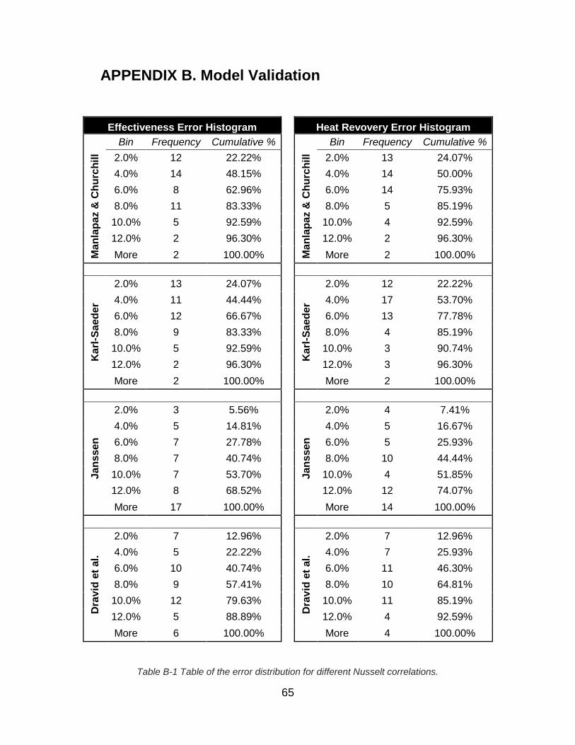
65

APPENDIX B. Model Validation

Effectiveness Error Histogram Heat Revovery Error Histogram

Bin Frequency Cumulative % Bin Frequency Cumulative %

Ma

nla

pa

z &

Ch

urc

hill 2.0% 12 22.22%

Ma

nla

pa

z &

Ch

urc

hill 2.0% 13 24.07%

4.0% 14 48.15% 4.0% 14 50.00%

6.0% 8 62.96% 6.0% 14 75.93%

8.0% 11 83.33% 8.0% 5 85.19%

10.0% 5 92.59% 10.0% 4 92.59%

12.0% 2 96.30% 12.0% 2 96.30%

More 2 100.00% More 2 100.00%

Ka

rl-S

aed

er

2.0% 13 24.07%

Ka

rl-S

aed

er

2.0% 12 22.22%

4.0% 11 44.44% 4.0% 17 53.70%

6.0% 12 66.67% 6.0% 13 77.78%

8.0% 9 83.33% 8.0% 4 85.19%

10.0% 5 92.59% 10.0% 3 90.74%

12.0% 2 96.30% 12.0% 3 96.30%

More 2 100.00% More 2 100.00%

Jan

ssen

2.0% 3 5.56%

Jan

ssen

2.0% 4 7.41%

4.0% 5 14.81% 4.0% 5 16.67%

6.0% 7 27.78% 6.0% 5 25.93%

8.0% 7 40.74% 8.0% 10 44.44%

10.0% 7 53.70% 10.0% 4 51.85%

12.0% 8 68.52% 12.0% 12 74.07%

More 17 100.00% More 14 100.00%

Dra

vid

et

al.

2.0% 7 12.96%

Dra

vid

et

al.

2.0% 7 12.96%

4.0% 5 22.22% 4.0% 7 25.93%

6.0% 10 40.74% 6.0% 11 46.30%

8.0% 9 57.41% 8.0% 10 64.81%

10.0% 12 79.63% 10.0% 11 85.19%

12.0% 5 88.89% 12.0% 4 92.59%

More 6 100.00% More 4 100.00%

Table B-1 Table of the error distribution for different Nusselt correlations.

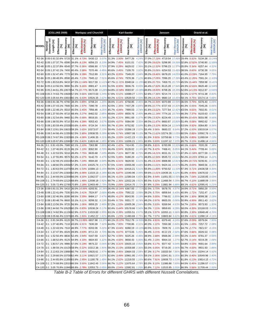
66

(COLLINS 2009) Manlapaz and Churchill Karl-Saeder Janssen Dravid et al.

MODEL N

om

ina

l

Dia

me

ter

[m]

Le

ng

th [

m]

Eff

ec

tive

ne

ss

[%]

Hea

t R

ec

ov

ery

[W]

Eff

ec

tive

ne

ss

[%]

Eff

ec

tive

ne

ss

ER

RO

R [

%]

Hea

t R

ec

ov

ery

[W]

Hea

t R

ec

ov

ery

ER

RO

R [

W]

Eff

ec

tive

ne

ss

[%]

Eff

ec

tive

ne

ss

ER

RO

R [

%]

Hea

t R

ec

ov

ery

[W]

Hea

t R

ec

ov

ery

ER

RO

R [

W]

Eff

ec

tive

ne

ss

[%]

Eff

ec

tive

ne

ss

ER

RO

R [

%]

Hea

t R

ec

ov

ery

[W]

Hea

t R

ec

ov

ery

ER

RO

R [

W]

Eff

ec

tive

ne

ss

[%]

Eff

ec

tive

ne

ss

ER

RO

R [

%]

Hea

t R

ec

ov

ery

[W]

Hea

t R

ec

ov

ery

ER

RO

R [

W]

R2-36 0.05 0.91 32.6% 5720 31.1% 4.73% 5430.13 5.07% 31.3% 3.90% 5477.26 4.24% 27.0% 17.19% 4719.54 17.49% 29.4% 9.92% 5134.38 10.24%

R2-42 0.05 1.07 37.7% 6590 34.6% 8.13% 6056.23 8.10% 34.9% 7.45% 6101.01 7.42% 30.3% 19.62% 5298.90 19.59% 32.8% 12.92% 5740.80 12.89%

R2-48 0.05 1.22 37.8% 6540 37.7% 0.36% 6586.90 0.72% 37.9% 0.28% 6629.02 1.36% 33.1% 12.32% 5796.23 11.37% 35.8% 5.34% 6257.44 4.32%

R2-54 0.05 1.37 42.1% 7400 40.4% 3.98% 7070.46 4.45% 40.6% 3.45% 7109.70 3.92% 35.8% 15.06% 6254.53 15.48% 38.5% 8.60% 6730.39 9.05%

R2-60 0.05 1.52 47.4% 7770 42.9% 9.39% 7512.89 3.31% 43.2% 8.95% 7549.20 2.84% 38.2% 19.46% 6678.20 14.05% 41.0% 13.59% 7164.95 7.79%

R2-66 0.05 1.68 48.9% 8590 45.4% 7.13% 7945.12 7.51% 45.6% 6.74% 7978.36 7.12% 40.6% 17.05% 7096.20 17.39% 43.4% 11.26% 7591.24 11.63%

R2-72 0.05 1.83 53.8% 9410 47.5% 11.64% 8317.59 11.61% 47.7% 11.31% 8348.04 11.29% 42.6% 20.75% 7459.70 20.73% 45.5% 15.44% 7959.98 15.41%

R2-84 0.05 2.13 56.5% 9890 51.3% 9.16% 8981.47 9.19% 51.5% 8.90% 9006.76 8.93% 46.4% 17.92% 8115.28 17.94% 49.3% 12.81% 8620.48 12.84%

R2-96 0.05 2.44 61.3% 10670 54.7% 10.77% 9573.38 10.28% 54.8% 10.58% 9593.97 10.08% 49.8% 18.83% 8708.26 18.39% 52.6% 14.13% 9212.97 13.66%

R2-108 0.05 2.74 63.7% 10630 57.5% 9.66% 10072.63 5.24% 57.6% 9.51% 10089.27 5.09% 52.6% 17.36% 9214.74 13.31% 55.5% 12.87% 9715.38 8.60%

R2-120 0.05 3.05 64.4% 10810 60.1% 6.63% 10526.35 2.62% 60.2% 6.51% 10539.50 2.50% 55.3% 14.13% 9680.14 10.45% 58.1% 9.75% 10174.14 5.88%

R3-36 0.08 0.91 38.7% 6790 38.4% 0.89% 6708.24 1.20% 38.6% 0.14% 6758.85 0.46% 34.7% 10.30% 6070.89 10.59% 36.5% 5.79% 6376.40 6.09%

R3-42 0.08 1.07 43.1% 7500 42.3% 1.97% 7390.78 1.46% 42.5% 1.35% 7437.29 0.84% 38.5% 10.77% 6727.43 10.30% 40.3% 6.55% 7045.26 6.06%

R3-48 0.08 1.22 48.1% 8310 45.5% 5.45% 7956.46 4.25% 45.7% 4.94% 7999.03 3.74% 41.6% 13.52% 7277.64 12.42% 43.5% 9.65% 7602.81 8.51%

R3-54 0.08 1.37 50.0% 8710 48.4% 3.27% 8462.02 2.85% 48.6% 2.83% 8500.76 2.40% 44.4% 11.14% 7774.16 10.74% 46.3% 7.37% 8103.63 6.96%

R3-60 0.08 1.52 54.6% 9460 51.0% 6.68% 8916.55 5.74% 51.2% 6.31% 8951.69 5.37% 47.0% 13.92% 8224.49 13.06% 48.9% 10.45% 8555.98 9.56%

R3-66 0.08 1.68 55.9% 9710 53.4% 4.39% 9353.43 3.67% 53.6% 4.07% 9384.99 3.35% 49.5% 11.47% 8660.87 10.80% 51.4% 8.08% 8992.62 7.39%

R3-72 0.08 1.83 59.4% 10330 55.6% 6.46% 9724.34 5.86% 55.7% 6.19% 9752.82 5.59% 51.6% 13.10% 9034.14 12.54% 53.5% 9.92% 9364.80 9.34%

R3-84 0.08 2.13 61.5% 10610 59.3% 3.65% 10373.07 2.23% 59.4% 3.43% 10396.19 2.02% 55.4% 9.96% 9693.22 8.64% 57.2% 6.93% 10019.04 5.57%

R3-96 0.08 2.44 66.4% 11550 62.5% 5.90% 10938.55 5.29% 62.6% 5.74% 10957.08 5.13% 58.7% 11.62% 10274.28 11.05% 60.5% 8.88% 10592.76 8.29%

R3-108 0.08 2.74 67.9% 11920 65.1% 4.06% 11406.35 4.31% 65.2% 3.93% 11421.23 4.18% 61.5% 9.50% 10759.66 9.73% 63.2% 6.89% 11069.84 7.13%

R3-120 0.08 3.05 67.8% 12060 67.5% 0.40% 11824.44 1.95% 67.6% 0.30% 11836.21 1.86% 63.9% 5.69% 11197.12 7.15% 65.7% 3.15% 11498.14 4.66%

R4-36 0.1 0.91 43.0% 7580 42.1% 2.10% 7363.98 2.85% 42.4% 1.42% 7414.95 2.18% 38.8% 9.81% 6783.99 10.50% 40.1% 6.66% 7020.28 7.38%

R4-42 0.1 1.07 46.6% 8120 46.1% 1.10% 8062.90 0.70% 46.4% 0.54% 8109.02 0.14% 42.7% 8.42% 7466.41 8.05% 44.1% 5.44% 7709.44 5.06%

R4-48 0.1 1.22 53.5% 9310 49.4% 7.75% 8635.68 7.24% 49.6% 7.31% 8677.39 6.79% 45.9% 14.21% 8031.31 13.73% 47.3% 11.58% 8277.59 11.09%

R4-54 0.1 1.37 55.8% 9570 52.2% 6.37% 9142.70 4.47% 52.5% 5.99% 9180.29 4.07% 48.8% 12.59% 8535.72 10.81% 50.2% 10.05% 8783.14 8.22%

R4-60 0.1 1.52 59.1% 10310 54.8% 7.24% 9594.69 6.94% 55.0% 6.91% 9628.50 6.61% 51.4% 13.10% 8988.88 12.81% 52.8% 10.71% 9235.91 10.42%

R4-66 0.1 1.68 60.5% 10550 57.3% 5.33% 10025.74 4.97% 57.5% 5.04% 10055.90 4.68% 53.8% 11.01% 9424.16 10.67% 55.2% 8.69% 9669.56 8.35%

R4-72 0.1 1.83 63.5% 11070 59.3% 6.54% 10389.13 6.15% 59.5% 6.29% 10416.21 5.91% 55.9% 11.89% 9793.52 11.53% 57.3% 9.71% 10036.58 9.34%

R4-84 0.1 2.13 67.0% 11500 62.9% 6.06% 11019.13 4.18% 63.1% 5.87% 11040.96 3.99% 59.6% 11.01% 10439.16 9.22% 61.0% 8.99% 10676.02 7.17%

R4-96 0.1 2.44 69.0% 12300 66.0% 4.30% 11562.57 6.00% 66.1% 4.15% 11580.04 5.85% 62.8% 8.94% 11001.55 10.56% 64.1% 7.04% 11230.85 8.69%

R4-108 0.1 2.74 69.6% 12120 68.6% 1.48% 12008.19 0.92% 68.7% 1.36% 12022.26 0.81% 65.5% 5.92% 11466.54 5.39% 66.7% 4.10% 11688.09 3.56%

R4-120 0.1 3.05 72.4% 12760 70.8% 2.18% 12403.49 2.79% 70.9% 2.09% 12414.70 2.71% 67.8% 6.29% 11881.94 6.88% 69.1% 4.61% 12095.41 5.21%

C3-36 0.08 0.91 31.3% 5410 36.0% 14.99% 6293.91 16.34% 36.4% 16.34% 6367.93 17.71% 32.5% 3.75% 5678.76 4.97% 34.0% 8.71% 5950.29 9.99%

C3-48 0.08 1.22 41.6% 7330 43.0% 3.41% 7524.97 2.66% 43.4% 4.33% 7592.22 3.58% 39.2% 5.75% 6858.64 6.43% 40.9% 1.71% 7152.47 2.42%

C3-60 0.08 1.52 46.9% 8280 48.5% 3.39% 8484.17 2.47% 48.8% 4.12% 8543.95 3.19% 44.6% 5.00% 7796.01 5.85% 46.3% 1.30% 8099.38 2.18%

C3-72 0.08 1.83 48.7% 8600 53.1% 9.11% 9299.32 8.13% 53.4% 9.73% 9351.77 8.74% 49.2% 0.97% 8605.55 0.06% 50.9% 4.56% 8911.43 3.62%

C3-84 0.08 2.13 56.3% 9720 56.9% 1.06% 9959.25 2.46% 57.2% 1.53% 10005.36 2.94% 53.0% 5.93% 9269.94 4.63% 54.7% 2.85% 9573.93 1.50%

C3-96 0.08 2.44 60.7% 10520 60.2% 0.83% 10538.24 0.17% 60.4% 0.44% 10578.66 0.56% 56.3% 7.21% 9859.65 6.28% 58.0% 4.39% 10159.03 3.43%

C3-108 0.08 2.74 62.9% 11130 62.9% 0.07% 11019.83 0.99% 63.1% 0.39% 11055.51 0.67% 59.1% 5.97% 10355.11 6.96% 60.8% 3.30% 10648.49 4.33%

C3-120 0.08 3.05 66.4% 11570 65.4% 1.50% 11452.22 1.02% 65.6% 1.23% 11483.69 0.75% 61.7% 7.07% 10803.84 6.62% 63.3% 4.61% 11090.14 4.15%

C4-36 0.1 0.91 34.8% 6120 39.7% 13.99% 6937.98 13.37% 40.1% 15.22% 7012.79 14.59% 36.5% 4.81% 6379.40 4.24% 37.6% 8.09% 6579.04 7.50%

C4-42 0.1 1.07 40.8% 7110 43.6% 6.91% 7630.39 7.32% 44.0% 7.90% 7700.86 8.31% 40.3% 1.22% 7050.38 0.84% 41.5% 1.69% 7257.72 2.08%

C4-48 0.1 1.22 43.5% 7510 46.9% 7.77% 8202.06 9.22% 47.3% 8.64% 8268.19 10.10% 43.5% 0.01% 7609.76 1.33% 44.7% 2.77% 7821.57 4.15%

C4-54 0.1 1.37 47.9% 8320 49.8% 3.93% 8711.23 4.70% 50.1% 4.67% 8773.05 5.45% 46.4% 3.21% 8112.23 2.50% 47.6% 0.66% 8326.53 0.08%

C4-60 0.1 1.52 50.4% 8830 52.4% 3.94% 9167.59 3.82% 52.7% 4.59% 9225.26 4.48% 48.9% 2.88% 8566.06 2.99% 50.2% 0.44% 8781.37 0.55%

C4-66 0.1 1.68 52.6% 9120 54.9% 4.33% 9604.93 5.32% 55.2% 4.92% 9658.43 5.90% 51.4% 2.19% 9004.10 1.27% 52.7% 0.14% 9219.28 1.09%

C4-72 0.1 1.83 57.1% 9980 57.0% 0.19% 9975.22 0.05% 57.3% 0.31% 10025.10 0.45% 53.6% 6.17% 9377.42 6.04% 54.8% 4.03% 9591.64 3.89%

C4-78 0.1 1.98 59.1% 10120 58.9% 0.32% 10312.36 1.90% 59.2% 0.13% 10358.88 2.36% 55.5% 6.05% 9719.30 3.96% 56.7% 4.00% 9931.93 1.86%

C4-84 0.1 2.13 63.1% 10890 60.7% 3.85% 10620.61 2.47% 60.9% 3.46% 10664.03 2.08% 57.3% 9.17% 10033.54 7.86% 58.5% 7.26% 10244.14 5.93%

C4-90 0.1 2.29 60.5% 10700 62.4% 3.11% 10921.57 2.07% 62.6% 3.49% 10961.95 2.45% 59.1% 2.36% 10341.91 3.35% 60.3% 0.40% 10549.96 1.40%

C4-96 0.1 2.44 65.8% 11350 63.9% 2.95% 11180.78 1.49% 64.1% 2.62% 11218.55 1.16% 60.6% 7.91% 10608.73 6.53% 61.8% 6.13% 10814.15 4.72%

C4-108 0.1 2.74 68.9% 12010 66.5% 3.50% 11642.45 3.06% 66.7% 3.22% 11675.64 2.78% 63.3% 8.10% 11086.86 7.69% 64.5% 6.45% 11286.57 6.02%

C4-120 0.1 3.05 70.8% 11940 68.8% 2.78% 12053.73 0.95% 69.0% 2.54% 12082.91 1.20% 65.8% 7.12% 11515.95 3.55% 66.9% 5.56% 11709.44 1.93%

Table B-2 Table of Errors for different GHRS with different Nusselt Correlations.

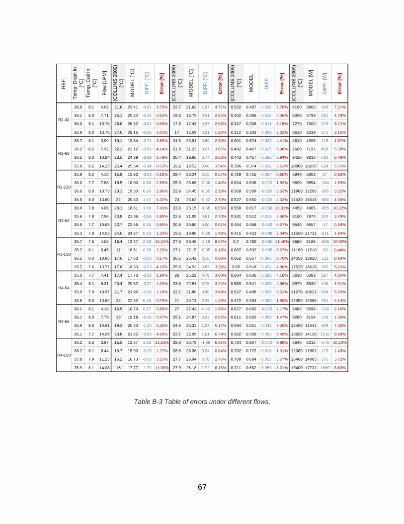
67

Table B-3 Table of errors under different flows.

RE

F.

Tem

p. D

rain

In

[°C

]

Tem

p. C

oil

In

[°C

]

Flo

w [LP

M]

(CO

LLIN

S 2

009)

[°C

]

MO

DE

L [°C

]

DIF

F. [°

C]

Err

or

[%]

(CO

LLIN

S 2

009)

[°C

]

MO

DE

L [°C

]

DIF

F. [°

C]

Err

or

[%]

(CO

LLIN

S 2

009)

[°C

]

MO

DE

L

DIF

F.

Err

or

[%]

(CO

LLIN

S 2

009)

[°C

]

MO

DE

L [W

]

DIF

F. [W

]

Err

or

[%]

36.0 8.1 4.03 21.6 22.41 -0.81 3.75% 22.7 21.63 1.07 4.71% 0.522 0.487 0.035 6.76% 4100 3800 300 7.31%

36.1 8.0 7.71 25.1 25.24 -0.14 0.54% 19.3 18.79 0.51 2.64% 0.402 0.386 0.016 4.06% 6090 5799 291 4.78%

36.0 8.1 10.76 26.6 26.62 -0.02 0.09% 17.8 17.43 0.37 2.06% 0.347 0.336 0.011 3.15% 7270 7000 270 3.71%

36.9 8.0 13.75 27.6 28.16 -0.56 2.01% 17 16.69 0.31 1.82% 0.312 0.303 0.009 3.02% 8610 8339 271 3.15%

35.7 8.1 3.99 19.1 19.84 -0.74 3.89% 24.6 23.91 0.69 2.80% 0.601 0.574 0.027 4.41% 4610 4395 215 4.67%

36.2 8.2 7.92 22.2 23.12 -0.92 4.14% 21.9 21.23 0.67 3.05% 0.492 0.467 0.025 5.06% 7600 7191 409 5.38%

36.1 8.0 10.84 23.5 24.39 -0.89 3.79% 20.4 19.66 0.74 3.62% 0.443 0.417 0.026 5.94% 9420 8810 610 6.48%

35.9 8.2 14.23 25.4 25.54 -0.14 0.53% 19.2 18.52 0.68 3.54% 0.396 0.374 0.022 5.51% 10860 10236 624 5.75%

35.9 8.2 4.16 15.8 15.83 -0.03 0.18% 28.4 28.24 0.16 0.57% 0.729 0.725 0.004 0.60% 5840 5803 37 0.63%

36.0 7.7 7.88 18.5 18.00 0.50 2.69% 25.3 25.66 -0.36 1.40% 0.624 0.636 -0.012 1.92% 9690 9854 -164 1.69%

36.0 8.0 10.73 20.1 19.50 0.60 2.96% 23.9 24.45 -0.55 2.30% 0.569 0.589 -0.020 3.53% 11900 12295 -395 3.32%

36.5 8.0 13.80 22 20.83 1.17 5.32% 23 23.62 -0.62 2.70% 0.527 0.550 -0.023 4.32% 14430 15016 -586 4.06%

36.0 7.8 4.06 20.1 18.61 1.49 7.41% 23.6 25.15 -1.55 6.55% 0.559 0.617 -0.058 10.31% 4450 4905 -455 10.22%

35.6 7.8 7.96 20.8 21.36 -0.56 2.69% 22.6 21.99 0.61 2.70% 0.531 0.512 0.019 3.56% 8180 7870 310 3.79%

35.5 7.7 10.63 22.7 22.55 0.15 0.65% 20.6 20.60 0.00 0.01% 0.464 0.466 -0.002 0.37% 9540 9557 -17 0.18%

36.3 7.9 14.03 24.6 24.27 0.33 1.33% 19.6 19.88 -0.28 1.42% 0.415 0.423 -0.008 2.04% 11500 11711 -211 1.84%

35.7 7.6 4.06 16.4 13.77 2.63 16.04% 27.3 29.49 -2.19 8.02% 0.7 0.780 -0.080 11.46% 5580 6188 -608 10.90%

35.7 8.1 8.45 17 16.61 0.39 2.29% 27.1 27.15 -0.05 0.18% 0.687 0.692 -0.005 0.67% 11160 11210 -50 0.44%

36.1 8.0 10.85 17.6 17.63 -0.03 0.17% 26.6 26.42 0.18 0.68% 0.662 0.657 0.005 0.76% 14050 13920 131 0.93%

35.7 7.6 13.77 17.6 18.33 -0.73 4.15% 25.8 24.93 0.87 3.38% 0.65 0.618 0.032 4.90% 17520 16618 902 5.15%

35.3 7.7 4.41 17.4 17.73 -0.33 1.90% 26 25.22 0.78 3.00% 0.664 0.636 0.028 4.16% 5610 5383 227 4.05%

35.4 8.1 8.31 20.4 20.62 -0.22 1.09% 23.6 22.84 0.76 3.24% 0.569 0.541 0.028 4.86% 8970 8530 440 4.91%

35.9 7.9 10.97 21.7 21.96 -0.26 1.18% 22.7 21.80 0.90 3.98% 0.527 0.498 0.029 5.51% 11270 10621 649 5.76%

35.6 8.0 13.62 23 22.82 0.18 0.79% 21 20.74 0.26 1.26% 0.472 0.463 0.009 1.89% 12350 12086 264 2.14%

36.1 8.1 4.16 16.9 16.73 0.17 0.99% 27 27.42 -0.42 1.56% 0.677 0.692 -0.015 2.17% 5480 5598 -118 2.16%

36.1 8.0 7.79 19 19.18 -0.18 0.97% 25.1 24.87 0.23 0.92% 0.611 0.602 0.009 1.47% 9280 9154 126 1.36%

35.9 8.0 10.81 19.3 20.53 -1.23 6.36% 24.6 23.33 1.27 5.17% 0.594 0.551 0.043 7.26% 12450 11541 909 7.30%

36.1 7.7 14.09 20.8 21.65 -0.85 4.09% 23.7 22.09 1.61 6.79% 0.562 0.509 0.053 9.49% 15650 14135 1516 9.68%

36.2 8.3 3.97 15.5 13.67 1.83 11.81% 28.8 30.79 -1.99 6.91% 0.734 0.807 -0.073 9.98% 5640 6216 -576 10.20%

36.2 8.1 8.44 15.7 15.90 -0.20 1.27% 28.6 28.36 0.24 0.84% 0.732 0.722 0.010 1.31% 12080 11907 173 1.43%

35.8 7.9 11.23 16.2 16.73 -0.53 3.25% 27.7 26.94 0.76 2.76% 0.709 0.684 0.025 3.57% 15460 14885 575 3.72%

35.9 8.1 14.08 16 17.77 -1.77 11.06% 27.9 26.18 1.72 6.16% 0.711 0.652 0.059 8.31% 19400 17731 1669 8.60%

R4-66

R4-120

R2-42

R2-60

R2-120

R3-54

R3-120

R4-54

68

APPENDIX C. Model simulations G

EO

ME

TR

Y

Le

ng

th [

m]

Eff

ec

tive

ne

ss

q [

kW

]

Td

rain

_o

ut

[°C

]

Tc

oil_

ou

t [°

C]

NT

U

UA

[W

/K]

ReD

rain

ReC

oil

Reg

ime

Co

il

R1 [

K/W

]

R2 [

K/W

]

R3 [

K/W

]

R4 [

K/W

]

R5 [

K/W

]

Rto

tal [K

/W]

Cco

il

Cd

rain

No

min

al

Dia

me

ter

= 0

.05

[m

]

Nu

mb

er

of

co

ils

= 2

0.91 34.35% 6.01 26.38 17.57 0.523 326.4 4887.3 9877.1 Laminar 1.54E-03 3.36E-05 2.59E-04 3.27E-05 1.20E-03 3.06E-03 627.37 624.49

1.07 38.06% 6.66 25.34 18.61 0.614 383.3 4834.8 10017.5 Laminar 1.32E-03 2.85E-05 2.20E-04 2.78E-05 1.01E-03 2.61E-03 627.28 624.60

1.22 41.18% 7.20 24.47 19.48 0.699 436.7 4791.0 10135.9 Laminar 1.17E-03 2.50E-05 1.93E-04 2.44E-05 8.80E-04 2.29E-03 627.20 624.69

1.37 43.99% 7.70 23.68 20.27 0.784 489.9 4751.5 10243.2 Laminar 1.05E-03 2.23E-05 1.72E-04 2.17E-05 7.79E-04 2.04E-03 627.14 624.77

1.52 46.54% 8.14 22.97 20.98 0.869 543.1 4715.8 10341.0 Laminar 9.48E-04 2.01E-05 1.55E-04 1.96E-05 6.99E-04 1.84E-03 627.08 624.84

1.68 49.01% 8.58 22.28 21.68 0.960 599.7 4681.3 10436.1 Laminar 8.62E-04 1.82E-05 1.40E-04 1.77E-05 6.29E-04 1.67E-03 627.03 624.91

1.83 51.13% 8.95 21.68 22.27 1.044 652.7 4651.8 10517.8 Laminar 7.95E-04 1.67E-05 1.29E-04 1.62E-05 5.75E-04 1.53E-03 626.99 624.97

2.13 54.87% 9.60 20.64 23.32 1.214 758.6 4599.9 10662.7 Laminar 6.89E-04 1.43E-05 1.11E-04 1.40E-05 4.90E-04 1.32E-03 626.91 625.06

2.44 58.17% 10.18 19.71 24.24 1.388 867.7 4554.2 10791.2 Laminar 6.06E-04 1.25E-05 9.66E-05 1.22E-05 4.25E-04 1.15E-03 626.85 625.15

2.74 60.93% 10.67 18.94 25.02 1.556 973.1 4516.2 10899.1 Laminar 5.43E-04 1.11E-05 8.61E-05 1.08E-05 3.76E-04 1.03E-03 626.80 625.22

3.05 63.42% 11.10 18.24 25.72 1.730 1081.9 4482.0 10996.9 Laminar 4.91E-04 1.00E-05 7.73E-05 9.75E-06 3.37E-04 9.24E-04 626.75 625.28

No

min

al

Dia

me

ter

= 0

.05

[m

]

Nu

mb

er

of

co

ils

= 4

0.91 31.06% 5.43 27.30 16.65 0.450 281.0 4933.9 4876.6 Laminar 1.53E-03 3.36E-05 2.59E-04 3.27E-05 1.70E-03 3.56E-03 627.46 624.40

1.07 34.63% 6.06 26.30 17.65 0.529 330.5 4883.3 4943.9 Laminar 1.31E-03 2.85E-05 2.20E-04 2.78E-05 1.44E-03 3.03E-03 627.36 624.50

1.22 37.66% 6.59 25.45 18.50 0.603 376.9 4840.4 5001.2 Laminar 1.16E-03 2.50E-05 1.93E-04 2.44E-05 1.25E-03 2.65E-03 627.29 624.59

1.37 40.42% 7.07 24.68 19.27 0.678 423.3 4801.6 5053.6 Laminar 1.04E-03 2.23E-05 1.72E-04 2.17E-05 1.11E-03 2.36E-03 627.22 624.67

1.52 42.95% 7.51 23.97 19.98 0.752 469.6 4766.1 5101.8 Laminar 9.41E-04 2.01E-05 1.55E-04 1.96E-05 9.94E-04 2.13E-03 627.16 624.74

1.68 45.41% 7.95 23.28 20.67 0.831 519.0 4731.5 5148.9 Laminar 8.56E-04 1.82E-05 1.40E-04 1.77E-05 8.95E-04 1.93E-03 627.11 624.81

1.83 47.54% 8.32 22.69 21.26 0.905 565.3 4701.8 5189.7 Laminar 7.89E-04 1.67E-05 1.29E-04 1.62E-05 8.18E-04 1.77E-03 627.06 624.87

2.13 51.33% 8.98 21.63 22.32 1.053 657.9 4649.1 5262.7 Laminar 6.84E-04 1.43E-05 1.11E-04 1.40E-05 6.97E-04 1.52E-03 626.99 624.97

2.44 54.70% 9.57 20.68 23.27 1.205 753.4 4602.2 5328.1 Laminar 6.01E-04 1.25E-05 9.66E-05 1.22E-05 6.05E-04 1.33E-03 626.92 625.06

2.74 57.55% 10.07 19.89 24.07 1.353 845.8 4562.9 5383.4 Laminar 5.39E-04 1.11E-05 8.61E-05 1.08E-05 5.35E-04 1.18E-03 626.86 625.13

3.05 60.13% 10.53 19.16 24.79 1.505 941.1 4527.2 5433.9 Laminar 4.87E-04 1.00E-05 7.73E-05 9.75E-06 4.78E-04 1.06E-03 626.81 625.20

No

min

al

Dia

me

ter

= 0

.05

[m

]

Nu

mb

er

of

co

ils

= 6

0.91 28.92% 5.06 27.90 16.06 0.406 253.8 4964.3 3224.4 Laminar 1.52E-03 3.36E-05 2.59E-04 3.27E-05 2.09E-03 3.94E-03 627.52 624.33

1.07 32.38% 5.66 26.93 17.02 0.478 298.7 4915.2 3267.7 Laminar 1.31E-03 2.85E-05 2.20E-04 2.78E-05 1.77E-03 3.35E-03 627.42 624.44

1.22 35.34% 6.18 26.11 17.85 0.546 340.9 4873.3 3304.8 Laminar 1.15E-03 2.50E-05 1.93E-04 2.44E-05 1.54E-03 2.93E-03 627.34 624.52

1.37 38.04% 6.65 25.35 18.61 0.613 383.0 4835.1 3338.9 Laminar 1.03E-03 2.23E-05 1.72E-04 2.17E-05 1.36E-03 2.61E-03 627.28 624.60

1.52 40.53% 7.09 24.65 19.30 0.681 425.2 4800.0 3370.5 Laminar 9.36E-04 2.01E-05 1.55E-04 1.96E-05 1.22E-03 2.35E-03 627.22 624.67

1.68 42.98% 7.52 23.97 19.99 0.753 470.2 4765.7 3401.5 Laminar 8.51E-04 1.82E-05 1.40E-04 1.77E-05 1.10E-03 2.13E-03 627.16 624.74

1.83 45.09% 7.89 23.37 20.58 0.820 512.3 4736.0 3428.5 Laminar 7.85E-04 1.67E-05 1.29E-04 1.62E-05 1.01E-03 1.95E-03 627.12 624.80

2.13 48.88% 8.55 22.31 21.64 0.955 596.7 4683.1 3477.1 Laminar 6.80E-04 1.43E-05 1.11E-04 1.40E-05 8.57E-04 1.68E-03 627.04 624.90

2.44 52.29% 9.15 21.36 22.60 1.094 683.8 4635.7 3520.9 Laminar 5.98E-04 1.25E-05 9.66E-05 1.22E-05 7.43E-04 1.46E-03 626.97 625.00

2.74 55.18% 9.66 20.55 23.40 1.229 768.1 4595.6 3558.2 Laminar 5.36E-04 1.11E-05 8.61E-05 1.08E-05 6.58E-04 1.30E-03 626.91 625.07

3.05 57.81% 10.12 19.81 24.14 1.368 855.2 4559.1 3592.5 Laminar 4.84E-04 1.00E-05 7.73E-05 9.75E-06 5.88E-04 1.17E-03 626.86 625.14

No

min

al

Dia

me

ter

= 0

.08

[m

]

Nu

mb

er

of

co

ils

= 4

0.91 38.36% 6.71 25.26 18.69 0.621 388.1 3019.2 5014.3 Laminar 1.14E-03 2.13E-05 1.67E-04 2.13E-05 1.23E-03 2.58E-03 627.27 624.61

1.07 42.25% 7.39 24.17 19.78 0.731 456.4 2984.9 5088.5 Laminar 9.75E-04 1.81E-05 1.42E-04 1.81E-05 1.04E-03 2.19E-03 627.18 624.72

1.22 45.48% 7.96 23.27 20.69 0.833 520.4 2956.6 5150.2 Laminar 8.61E-04 1.59E-05 1.24E-04 1.59E-05 9.04E-04 1.92E-03 627.11 624.81

1.37 48.36% 8.46 22.46 21.50 0.935 584.3 2931.5 5205.6 Laminar 7.72E-04 1.41E-05 1.11E-04 1.41E-05 8.01E-04 1.71E-03 627.05 624.89

1.52 50.95% 8.92 21.73 22.22 1.037 648.2 2908.9 5255.5 Laminar 7.00E-04 1.27E-05 9.97E-05 1.27E-05 7.18E-04 1.54E-03 626.99 624.96

1.68 53.45% 9.35 21.04 22.92 1.146 716.3 2887.3 5303.7 Laminar 6.37E-04 1.15E-05 9.02E-05 1.15E-05 6.46E-04 1.40E-03 626.94 625.03

1.83 55.56% 9.72 20.44 23.51 1.248 780.1 2868.9 5344.8 Laminar 5.87E-04 1.06E-05 8.28E-05 1.06E-05 5.91E-04 1.28E-03 626.90 625.08

2.13 59.26% 10.37 19.41 24.55 1.452 907.6 2837.0 5416.9 Laminar 5.09E-04 9.09E-06 7.12E-05 9.09E-06 5.04E-04 1.10E-03 626.83 625.18

2.44 62.48% 10.94 18.51 25.45 1.662 1039.1 2809.3 5480.0 Laminar 4.47E-04 7.94E-06 6.21E-05 7.94E-06 4.37E-04 9.62E-04 626.77 625.26

2.74 65.15% 11.41 17.76 26.20 1.865 1166.3 2786.5 5532.4 Laminar 4.01E-04 7.07E-06 5.53E-05 7.07E-06 3.87E-04 8.57E-04 626.72 625.33

3.05 67.53% 11.82 17.09 26.87 2.075 1297.7 2766.1 5579.4 Laminar 3.62E-04 6.35E-06 4.97E-05 6.35E-06 3.46E-04 7.71E-04 626.68 625.38

No

min

al

Dia

me

ter

= 0

.08

[m

]

Nu

mb

er

of

co

ils

= 6

0.91 35.99% 6.29 25.92 18.03 0.562 350.7 3040.0 3313.0 Laminar 1.13E-03 2.13E-05 1.67E-04 2.13E-05 1.51E-03 2.85E-03 627.33 624.54

1.07 39.82% 6.96 24.85 19.10 0.661 412.8 3006.3 3361.4 Laminar 9.70E-04 1.81E-05 1.42E-04 1.81E-05 1.27E-03 2.42E-03 627.24 624.65

1.22 43.02% 7.52 23.96 20.00 0.754 470.9 2978.2 3402.0 Laminar 8.57E-04 1.59E-05 1.24E-04 1.59E-05 1.11E-03 2.12E-03 627.16 624.74

1.37 45.89% 8.03 23.15 20.80 0.847 529.1 2953.0 3438.7 Laminar 7.68E-04 1.41E-05 1.11E-04 1.41E-05 9.83E-04 1.89E-03 627.10 624.82

1.52 48.49% 8.48 22.42 21.53 0.940 587.3 2930.4 3472.0 Laminar 6.96E-04 1.27E-05 9.97E-05 1.27E-05 8.82E-04 1.70E-03 627.04 624.89

1.68 51.00% 8.92 21.72 22.23 1.039 649.3 2908.5 3504.2 Laminar 6.33E-04 1.15E-05 9.02E-05 1.15E-05 7.94E-04 1.54E-03 626.99 624.96

1.83 53.14% 9.30 21.12 22.83 1.132 707.5 2889.9 3531.8 Laminar 5.84E-04 1.06E-05 8.28E-05 1.06E-05 7.25E-04 1.41E-03 626.95 625.02

2.13 56.90% 9.96 20.07 23.89 1.318 823.7 2857.4 3580.6 Laminar 5.06E-04 9.09E-06 7.12E-05 9.09E-06 6.19E-04 1.21E-03 626.88 625.12

2.44 60.20% 10.54 19.14 24.81 1.510 943.8 2828.9 3623.5 Laminar 4.45E-04 7.94E-06 6.21E-05 7.94E-06 5.36E-04 1.06E-03 626.81 625.20

2.74 62.94% 11.02 18.38 25.58 1.695 1059.9 2805.3 3659.4 Laminar 3.99E-04 7.07E-06 5.53E-05 7.07E-06 4.75E-04 9.43E-04 626.76 625.27

3.05 65.41% 11.45 17.69 26.27 1.887 1179.9 2784.2 3691.7 Laminar 3.60E-04 6.35E-06 4.97E-05 6.35E-06 4.25E-04 8.48E-04 626.72 625.33

69

GE

OM

ET

RY

Len

gth

[m

]

Eff

ecti

ven

ess

q [

kW

]

Td

rain

_o

ut

[°C

]

Tco

il_o

ut

[°C

]

NT

U

UA

[W

/K]

ReD

rain

ReC

oil

Reg

imeC

oil

R1 [

K/W

]

R2 [

K/W

]

R3 [

K/W

]

R4 [

K/W

]

R5 [

K/W

]

Rto

tal [K

/W]

Cco

il

Cd

rain

No

min

al

Dia

mete

r =

0.1

0 [

m]

N

um

ber

of

co

ils =

4

0.91 42.10% 7.36 24.21 19.74 0.726 453.6 2389.0 5085.5 Laminar 9.88E-04 1.71E-05 1.35E-04 1.73E-05 1.05E-03 2.20E-03 627.18 624.72

1.07 46.09% 8.06 23.10 20.86 0.854 533.3 2361.1 5161.8 Laminar 8.48E-04 1.45E-05 1.14E-04 1.47E-05 8.84E-04 1.88E-03 627.09 624.83

1.22 49.35% 8.64 22.18 21.77 0.973 608.0 2338.3 5224.6 Laminar 7.49E-04 1.28E-05 1.00E-04 1.29E-05 7.70E-04 1.64E-03 627.03 624.92

1.37 52.24% 9.14 21.37 22.58 1.092 682.6 2318.1 5280.5 Laminar 6.71E-04 1.14E-05 8.94E-05 1.15E-05 6.82E-04 1.47E-03 626.97 625.00

1.52 54.82% 9.59 20.65 23.30 1.211 757.1 2300.3 5330.4 Laminar 6.08E-04 1.02E-05 8.05E-05 1.03E-05 6.11E-04 1.32E-03 626.92 625.06

1.68 57.28% 10.03 19.96 23.99 1.338 836.6 2283.3 5378.2 Laminar 5.53E-04 9.27E-06 7.29E-05 9.35E-06 5.50E-04 1.20E-03 626.87 625.13

1.83 59.35% 10.39 19.38 24.57 1.457 911.0 2269.0 5418.6 Laminar 5.10E-04 8.51E-06 6.69E-05 8.59E-06 5.03E-04 1.10E-03 626.83 625.18

2.13 62.94% 11.02 18.38 25.58 1.695 1059.7 2244.3 5489.0 Laminar 4.42E-04 7.31E-06 5.75E-05 7.38E-06 4.29E-04 9.44E-04 626.76 625.27

2.44 66.04% 11.56 17.51 26.45 1.940 1213.3 2223.1 5549.9 Laminar 3.89E-04 6.38E-06 5.02E-05 6.44E-06 3.73E-04 8.24E-04 626.71 625.35

2.74 68.57% 12.01 16.80 27.16 2.177 1361.7 2205.7 5600.1 Laminar 3.48E-04 5.68E-06 4.47E-05 5.73E-06 3.30E-04 7.34E-04 626.66 625.41

3.05 70.82% 12.40 16.17 27.79 2.422 1515.0 2190.4 5644.7 Laminar 3.14E-04 5.10E-06 4.01E-05 5.15E-06 2.95E-04 6.60E-04 626.62 625.46

No

min

al

Dia

mete

r =

0.1

0 [

m]

Nu

mb

er

of

co

ils =

6

0.91 39.67% 6.94 24.89 19.06 0.657 410.1 2406.1 3359.5 Laminar 9.83E-04 1.71E-05 1.35E-04 1.73E-05 1.29E-03 2.44E-03 627.24 624.65

1.07 43.62% 7.63 23.79 20.17 0.773 482.6 2378.3 3409.7 Laminar 8.43E-04 1.45E-05 1.14E-04 1.47E-05 1.09E-03 2.07E-03 627.15 624.76

1.22 46.88% 8.20 22.87 21.08 0.881 550.6 2355.5 3451.4 Laminar 7.45E-04 1.28E-05 1.00E-04 1.29E-05 9.46E-04 1.82E-03 627.08 624.85

1.37 49.78% 8.71 22.06 21.89 0.990 618.5 2335.3 3488.6 Laminar 6.67E-04 1.14E-05 8.94E-05 1.15E-05 8.37E-04 1.62E-03 627.02 624.93

1.52 52.39% 9.17 21.33 22.62 1.098 686.5 2317.2 3522.1 Laminar 6.05E-04 1.02E-05 8.05E-05 1.03E-05 7.51E-04 1.46E-03 626.96 625.00

1.68 54.88% 9.60 20.63 23.32 1.214 758.9 2299.9 3554.4 Laminar 5.50E-04 9.27E-06 7.29E-05 9.35E-06 6.76E-04 1.32E-03 626.91 625.07

1.83 56.99% 9.98 20.04 23.91 1.323 826.8 2285.3 3581.7 Laminar 5.08E-04 8.51E-06 6.69E-05 8.59E-06 6.18E-04 1.21E-03 626.87 625.12

2.13 60.67% 10.62 19.01 24.94 1.539 962.5 2259.9 3629.6 Laminar 4.40E-04 7.31E-06 5.75E-05 7.38E-06 5.27E-04 1.04E-03 626.80 625.21

2.44 63.86% 11.18 18.12 25.84 1.763 1102.7 2238.0 3671.4 Laminar 3.87E-04 6.38E-06 5.02E-05 6.44E-06 4.57E-04 9.07E-04 626.74 625.29

2.74 66.49% 11.64 17.38 26.58 1.980 1238.2 2220.0 3705.9 Laminar 3.47E-04 5.68E-06 4.47E-05 5.73E-06 4.05E-04 8.08E-04 626.70 625.36

3.05 68.83% 12.05 16.73 27.24 2.204 1378.2 2204.0 3736.8 Laminar 3.13E-04 5.10E-06 4.01E-05 5.15E-06 3.62E-04 7.26E-04 626.65 625.42

Table C-1 Full table of simulation results for different GHE.

70

APPENDIX D. Potential of Implementation

Table D-1 Full table of persons per household in Sweden 2015.

Source: (SCB-Sweden 2016)

Number of

households

Percentage of

Households

Number of

persons

Percentage

of persons

Persons per

Household

Single w ithout

children 1,648,130 38.06% 1,648,130 17.19% 1.00

Single w ith 1

children aged 0-

24

137,691 3.18% 275,382 2.87% 2.00

Single w ith 2

children aged 0-

24

87,780 2.03% 263,340 2.75% 3.00

Single w ith 3 or

more children

aged 0-24

31,110 0.72% 136,536 1.42% 4.39

Single w ith 1

children aged 25

and older

43,983 1.02% 87,966 0.92% 2.00

Single w ith 2

children aged 25

and older

3,078 0.07% 9,234 0.10% 3.00

Single w ith 3 or

more children

aged 25 and

older

217 0.01% 897 0.01% 4.13

Cohabiting/marr

ied w ithout

children

1,075,485 24.84% 2,150,970 22.44% 2.00

Cohabiting w ith

1 children aged

0-24

310,969 7.18% 932,907 9.73% 3.00

Cohabiting w ith

2 children aged

0-24

446,962 10.32% 1,787,848 18.65% 4.00

Cohabiting w ith

3 or more

children aged 0-

24

177,499 4.10% 942,351 9.83% 5.31

Cohabiting w ith

1 children aged

25 and older

55,789 1.29% 167,367 1.75% 3.00

Cohabiting w ith

2 children aged

25 and older

4,942 0.11% 19,768 0.21% 4.00

Cohabiting w ith

3 or more

children aged 25

and older

378 0.01% 1,941 0.02% 5.13

Other

household

w ithout children

171,168 3.95% 445,408 4.65% 2.60

Other

household w ith

1 children aged

0-24

47,529 1.10% 193,852 2.02% 4.08

Other

household w ith

2 children aged

0-24

44,488 1.03% 232,659 2.43% 5.23

Other

household w ith

3 or more

children aged 0-

24

35,430 0.82% 258,651 2.70% 7.30

Other

household w ith

1 children aged

25 and older

6,724 0.16% 26,527 0.28% 3.95

Other

household w ith

2 children aged

25 and older

947 0.02% 4,753 0.05% 5.02

Other

household w ith

3 or more

children aged 25

and older

102 0.00% 647 0.01% 6.34

Total 4,330,401 9,587,134

71

Avg. Persons per household in Europe

Figure D.1. Average person per Household in Europe 2014.

Source: (Eurostat 2016)

72

APPENDIX E. Screenshots GUI MATLAB

73

74

75