Reservoir modeling and characterization

Reservoir modeling and characterization

Sigve Hamilton Aspelund

The origins of oil and gas and how they are The origins of oil and gas and how they are formedformed Kerogen is the lipid-rich part of organic matter that is insoluble in

common organic solvents (lipids are the more waxy parts of animals and some plants). The extractable part is known as bitumen.

Kerogen is converted to bitumen during the maturation process. The amount of extractable bitumen is a measure of the maturity of a source rock.

Bitumen becomes petroleum during migration. Petroleum is the liquid organic substance recovered in wells.

The origins of oil and gas and how they The origins of oil and gas and how they are formedare formed Crude oil is the naturally occurring liquid form of petroleum. Petroleum generation takes place as the breakdown of kerogen occurs

with rising temperature. Temperature and time are the most important factors affecting the

breakdown of kerogen.

The origins of oil and gas and how they are The origins of oil and gas and how they are formedformed As formation temperature rises on progressive burial an immature stage

is succeeded by stages of oil generation, oil conversion to gas or cracking (to make a wet gas with significant amounts of liquids) and finally dry gas (i.e., no associated liquids) generation.

Conventional Oil and GasConventional Oil and Gas

Conventional oil is a mixture of mainly pentanes and heavier hydrocarbons recoverable at a well from an underground reservoir and liquid at atmospheric pressure and temperature. Unlike bitumen, conventional oil flows through a well without stimulation and through a pipeline without processing or dilution.

Conventional oil production is now in the final stages of depletion in most mature oil fields. There is a need to implement advanced methods of oil recovery to maximize the production and to extend the economic life of the oil fields.

Unconventional oilUnconventional oil

Unconventional oil is petroleum produced or extracted using techniques other than the conventional (oil well) method.

Oil industries and governments across the globe are investing in unconventional oil sources due to the increasing scarcity of conventional oil reserves.

Although the depletion of such reserves is evident, unconventional oil production is a less efficient process and has greater environmental impacts than that of conventional oil production.

Sources of unconventional oilSources of unconventional oil

According to the International Energy Agency's Oil Market Report unconventional oil includes the following sources:

Oil shales Oil sands-based synthetic crudes and derivative products Coal-based liquid supplies Biomass-based liquid supplies Liquids arising from chemical processing of natural gas[1]

Sedimentary basins and the dynamic nature Sedimentary basins and the dynamic nature of Earth’s crustof Earth’s crust

What are sedimentary basins? Sedimentary basins are regions where considerable thicknesses of

sediments have accumulated (in places up to 20 km). Sedimentary basins are widespread both onshore and o shore. The ff

way in which they form was a matter of considerable debate until the last 20 years.

The advance in our understanding during this very short period is mainly due to the e orts of the oil industry.ff

Sedimentary basins and the dynamic nature of Sedimentary basins and the dynamic nature of Earth’s crustEarth’s crust


Basin classification schemes

Extensional basins, strike-slip basins, flexural basins, basins associated with subduction zones, mystery basins. There are many di erent ffclassification schemes for sedimentary basins but most are unwieldy and use rather spurious criteria . The most useful scheme (presented here) is very simple and is based on basin forming mechanisms. About 80% of the sedimentary basins on Earth have formed by extension of the plates (often termed lithospheric extension).


Most of the remaining 20% of basins were formed by flexure of the plates beneath various forms of loading (this class will be covered in the next lecture). Pull-apart or strike-slip basins are relatively small and form in association with bends in strike-slip faults, such as the San Andreas Fault or the North Anatolian Fault. Only a very small number of basins still defy explanation, although we suspect that at least some of these have a thermal origin.

Sedimentary basinSedimentary basin

A depression in the crust of the Earth formed by plate tectonic activity in which sediments accumulate. Continued deposition can cause further depression or subsidence. Sedimentary basins, or simply basins, vary from bowl-shaped to elongated troughs. If rich hydrocarbon source rocks occur in combination with appropriate depth and duration of burial, hydrocarbon generation can occur within the basin.

SedimentarySedimentary

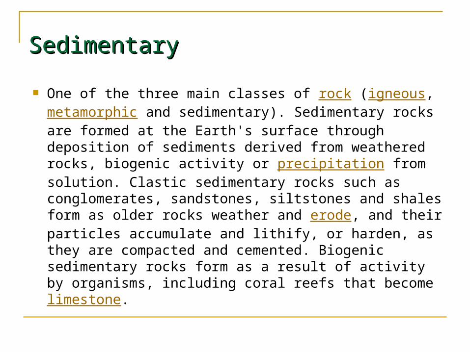
One of the three main classes of rock (igneous, metamorphic and sedimentary). Sedimentary rocks are formed at the Earth's surface through deposition of sediments derived from weathered rocks, biogenic activity or precipitation from solution. Clastic sedimentary rocks such as conglomerates, sandstones, siltstones and shales form as older rocks weather and erode, and their particles accumulate and lithify, or harden, as they are compacted and cemented. Biogenic sedimentary rocks form as a result of activity by organisms, including coral reefs that become limestone.

SedimentarySedimentary

Precipitates, such as the evaporite minerals halite (salt) and gypsum can form vast thicknesses of rock as seawater evaporates. Sedimentary rocks can include a wide variety of minerals, but quartz, feldspar, calcite, dolomite and evaporite group and clay group minerals are most common because of their greater stability at the Earth's surface than many minerals that comprise igneous and metamorphic rocks. Sedimentary rocks, unlike most igneous and metamorphic rocks, can contain fossils because they form at temperatures and pressures that do not obliterate fossil remnants.

Illustration of the rock cycleIllustration of the rock cycle

Concepts of finite resources and limitations Concepts of finite resources and limitations on recoveryon recovery

The Hubbert peak theory posits that for any given geographical area, from an individual oil-producing region to the planet as a whole, the rate of petroleum production tends to follow a bell-shaped curve. It is one of the primary theories on peak oil.

Choosing a particular curve determines a point of maximum production based on discovery rates, production rates and cumulative production. Early in the curve (pre-peak), the production rate increases because of the discovery rate and the addition of infrastructure. Late in the curve (post-peak), production declines because of resource depletion.

The Hubbert peak theory is based on the observation that the amount of oil under the ground in any region is finite, therefore the rate of discovery which initially increases quickly must reach a maximum and decline. In the US, oil extraction followed the discovery curve after a time lag of 32 to 35 years.[1][2]

The theory is named after American geophysicist M. King Hubbert, who created a method of modeling the production curve given an assumed ultimate recovery volume.

M. King Hubbert's original 1956 prediction 's original 1956 prediction of world petroleum production ratesof world petroleum production rates

Global distribution of fossil fuels and Global distribution of fossil fuels and OPEC’s resource endowmentOPEC’s resource endowment Reserves Around the World While most of the known oil and gas reserves are held in

the Middle East, they can be found in many places around the world, such as Australia, Italy, Malaysia and New Zealand. The leading petroleum producers include Saudi Arabia, Iran, Iraq, Kuwait and the United Arab Emirates. Oil is also produced in Russia, Canada, China, Brazil, Norway, Mexico, Venezuela, Great Britain, Nigeria and the United States — chiefly Texas, California, Louisiana, Oklahoma, Kansas and Alaska. Offshore reservoirs have been discovered in the North Sea, Africa, South America and the Gulf of Mexico.

• • Components that constitute natural gasComponents that constitute natural gas

Natural gas is a naturally occurring gas mixture consisting primarily of methane, typically with 0–20% higher hydrocarbons[1] (primarily ethane). It is found associated with other hydrocarbon fuel, in coal beds, as methane clathrates, and is an important fuel source and a major feedstock for fertilizers.

Most natural gas is created by two mechanisms: biogenic and thermogenic. Biogenic gas is created by methanogenic organisms in marshes, bogs, landfills, and shallow sediments. Deeper in the earth, at greater temperature and pressure, thermogenic gas is created from buried organic material.[2]

Before natural gas can be used as a fuel, it must undergo processing to remove almost all materials other than methane. The by-products of that processing include ethane, propane, butanes, pentanes, and higher molecular weight hydrocarbons, elemental sulfur, carbon dioxide, water vapor, and sometimes helium and nitrogen.

Natural gas is often informally referred to as simply gas, especially when compared to other energy sources such as oil or coal.

Uses and markets for oil and gasUses and markets for oil and gas

Who are the main consumers of oil? Nearly two thirds of global crude oil production is

consumed by the leading industrialised nations – i.e. the nations that make up the Organisation of Economic Cooperation and Development. But a rising share of oil demand is coming from the emerging market economies including China, Brazil, Russia and India.

BP Statistical Review of World Energy June 2012 For 61 years, the BP Statistical Review of

World Energy has provided high-quality objective and globally consistent data on world energy markets. The review is one of the most widely respected and authoritative publications in the fi eld of energy economics, used for reference by the media, academia, world governments and energy companies. A new edition is published every June.

Oil: Reserves to production

Oil: Distribution of proved reserves

Production and consumption by region

Consumption per capita 2011

Crude oil prices 1861-2011

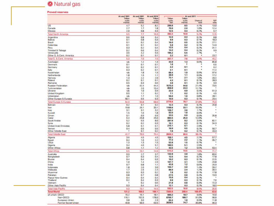
Gas: Reserves to production

Gas: Distribution of proved reserves

Gas: Production and consumption by region

Consumption per capita 2011

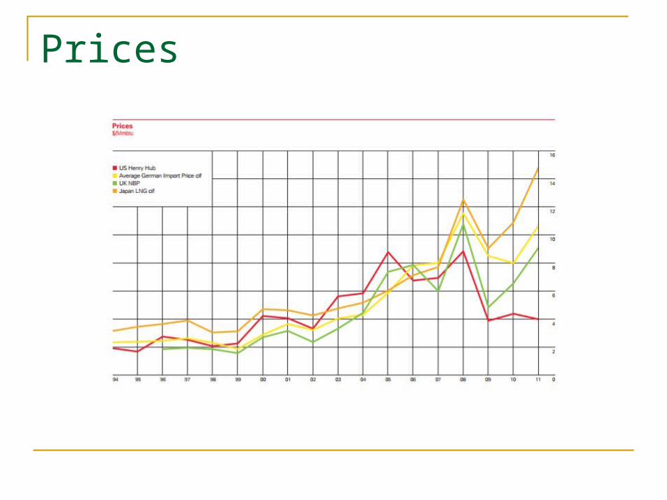
Prices

An introduction to petroleum geologyAn introduction to petroleum geology

Sedimentology The great majority of hydrocarbon reserves worldwide occur in

sedimentary rocks. It is therefore vitally important to understand the nature and distribution

of sediments as potential hydrocarbon source rocks and reservoirs. Two main groups of sedimentary rocks are of major importance as reservoirs, namely siltstones and sandstones (‘clastic’ sediments) and limestones and dolomites (‘carbonates’). Although carbonate rocks form the main reservoirs in certain parts of the world (e.g. in the Middle East, where a high proportion of the world’s giant oilfields are reservoired in carbonates), clastic rocks form the most significant reservoirs throughout most of the world.

CLASSIFICATION OF SEDIMENTARY CLASSIFICATION OF SEDIMENTARY ROCKSROCKS

Texture in Granular SedimentsTexture in Granular Sediments

The main textural components of granular rocks include: grain size grain sorting packing sediment fabric grain morphology grain surface texture

Grain sizeGrain size

SortingSorting

Grain shapeGrain shape

PackingPacking

Sand and sandstoneSand and sandstone

Sands are defined as sediments with a mean grain size between 0.0625 and 2 mm which, on compaction and cementation will become sandstones. Sandstones form the bulk of clastic hydrocarbon reservoirs, as they commonly have high porosities and permeabilities.

Sandstones are classified on the basis of their composition (mineralogical content) and texture (matrix content). The most common grains in sandstones are quartz, feldspar and fragments of older rocks. These rock fragments may include fragments of igneous, metamorphic and older sedimentary rocks.

Classification of sands and sandstonesClassification of sands and sandstones

Porosity Porosity

Total porosity (φ) is defined as the volume of void (pore) space within a rock, expressed as a fraction or percentage of the total rock volume. It is a measure of a rock’s fluid storage capacity.

The effective porosity of a rock is defined as the ratio of the interconnected pore volume to the bulk volume

Microporosity (φm) consists of pores less than 0.5 microns in size, whereas pores greater than 0.5 microns form macroporosity (φM)

PermeabilityPermeability

The permeability of a rock is a measure of its capacity to transmit a fluid under a potential gradient (pressure drop). The unit of permeability is the Darcy, which is defined by Darcy’s Law. The millidarcy (1/1000th Darcy) is generally used in core analysis.

Controls on Porosity and Controls on Porosity and PermeabilityPermeability The porosity and permeability of the sedimentary rock depend on both

the original texture of a sediment and its diagenetic history.

Grain sizeGrain size

In theory, porosity is independent of grain size, as it is merely a measure of the proportion of pore space in the rock, not the size of the pores. In practice, however, porosity tends to increase with decreasing grain size for two reasons. Finer grains, especially clays, tend to have less regular shapes than coarser grains, and so are often less efficiently packed. Also, fine sediments are commonly better sorted than coarser sediments. Both of these factors result in higher porosities.

For example, clays can have primary porosities of 50%-85% and fine sand can have 48% porosity whereas the primary porosity of coarse sand rarely exceeds 40%.

Permeability decreases with decreasing grain size because the size of pores and pore throats will also be smaller, leading to increased grain surface drag effects.

Porosity: Function of grain size and Porosity: Function of grain size and sortingsorting

Grain Shape The more unequidimensional the grain shape, the greater the porosity As permeability is a vector, rather than scalar property, grain shape will

affect the anisotropy of the permeability. The more unequidimensional the grains, the more anisotropic the permeability tensor.

Packing The closer the packing, the lower the porosity and permeability

Fabric Rock fabric will have the greatest influence on porosity and permeability

when the grains are non spherical (i.e. are either disc-like or rod-like). In these cases, the porosity and permeability of the sediment will decrease with increased alignment of the grains.

Grain Morphology and Surface Texture The smoother the grain surface, the higher the permeability

Diagenesis (e.g. Compaction, Diagenesis (e.g. Compaction, Cementation)Cementation)

Diagenesis is the totality of physical and chemical processes which occur after deposition of a sediment and during burial and which turn the sediment into a sedimentary rock. The majority of these processes, including compaction, cementation and the precipitation of authigenic clays, tend to reduce porosity and permeability, but others, such as grain or cement dissolution, may increase porosity and permeability. In general, porosity reduces exponentially with burial depth, but burial duration also an important criterion. Sediments that have spent a long time at great depths will tend to have lower porosities and permeabilities than those which have been rapidly buried.

Changes of porosity with burial Changes of porosity with burial depthdepth

Reservoir Rock & Source Rock Types: Classification Reservoir rock: A permeable subsurface

rock that contains petroleum. Must be both porous and permeable.

Source rock: A sedimentary rock in which petroleum forms.

Reservoir rocks are dominantly sedimentary (sandstones and carbonates); however, highly fractured igneous and metamorphic rocks have been known to produce hydrocarbons, albeit on a much smaller scale

Source rocks are widely agreed to be sedimentary The three sedimentary rock types most frequently encountered in

oil fields are shales, sandstones and carbonates Each of these rock types has a characteristic composition and

texture that is a direct result of depositional environment and post-depositional (diagenetic) processes (i.e., cementation, etc.)

Understanding reservoir rock properties and their associated characteristics is crucial in developing a prospect

Shales: Source rocks and seals Description

Distinctively dark-brown to black in color (occasionally a deep dark green), occasionally dark gray, with smooth lateral surfaces (normal to depositional direction)

Properties Composed of clay and silt-sized particles Clay particles are platy and orient themselves normal to

induced stress (overburden); this contributes to shale`s characteristic permeability

Behave as excellent seals Widely regarded to be the main source of hydrocarbons

due to original composition being rich in organics A weak rock highly susceptible to weathering and erosion

• History:• Deposited on river floodplaing, deep oceans, lakes or lagoons

• Occurrence:• The most abundant sedimentary rock (about 42%)

Sandstones and Sandstone ReservoirsDescription: Composed of sand-sized particles (q.v., week 2 notes) Recall that sandstones may contain textural features indicative of the environment in which

they were deposited: ripple marks (alluvial/fluvial), cross-bedding (alluvial/fluvial or eolian), gradedbedding (turbidity current)

Typically light beige to tan in color; can also be dark brown to rusty red Classification:

Sandstones can be further classified according to the abundance of grains of a particular chemical composition (i.e., common source rock); for example, an arkosic sanstone (usually abbreviated: ark. s.s.) is a sandstone largely composed of feldspar (feldspathic) grains….Can you recall which continental rock contains feldspar as one of its mineral constituents???

Sandstones composed of nearly all quartz grains are labeled quartz sandstones (usually abbreviated: qtz. s.s.)

Properties: Sandstone porosity is on the range of 10-30% Intergranular porosity is largely determined by sorting (primary porosity) Poorly indurated sandstones are referred to as fissile (easily disaggregated when

scratched), whereas highly indurated sandstones can be very resistant to weathering and erosion

Sandstone and sandstone reservoirs History: Sandstones are deposited in a number of different environments. These can include

deserts (e.g., wind-blown sands, i.e., eolian), stream valleys (e.g., alluvial/fluvial), and coastal/transitional environments (e.g., beach sands, barrier islands, deltas, turbidites)

Because of the wide variety of depositional environments in which sandstones can be found, care should be taken to observe textural features (i.e., grading, cross-bedding, etc.) within the reservoir that may provide evidence of its original diagenetic environment

Knowing the depositional environment of the s.s. reservoir is especially important in determining reservoir geometry and in anticipating potentially underpressured (commonly found in channel sandstones) and overpressured reservoir conditions

Occurrence: Are the second most abundant (about 37%) sedimentary rock type of the three

(sanstones, shales, carbonates), the most common reservoir rock, and are the second highest producer (about 37%)

Geologic Symbol: Dots or small circles randomly distributed; to include textural features, dots or circles may

be drawn to reflect the observation (for example, cross-bedding)

Carbonate and carbonate reservoirs Description Grains (clasts) are laregly the skeletal or shell remains of shallow

marine dwelling organisms, varying in size and shape, that either lived on the ocean bottom (benthic) or floated in water column (nerithic)

Many of these clasts can be identified by skilled paleontologists and micropaleontologists and can be used for correlative purposes or age range dating; also beneficial in establishing index fossils for marker beds used in regional stratigraphic correlations

Dolomites are a product of solution recrystallization of limestones Usually light or dark gray, abundant fossil molds and casts,

vuggy (vugular) porositity

Classification: Divided into limestones (Calsium carbonate-

CaCO3) and dolomites (Calcium magnesium carbonate – CaMg(CO3)2)

Limestones can be divided further into mudstones, wackenstones, packstones, grainstones and boundstones according to the limestones depositional texture

Properties: Porosity is largely a result of dissolution and fracturing (secondary porosity) Carbonates such as coquina are nearly 100% fossil fragments (largely primary

porosity) Are characteristically hard rocks, especially dolomite Susceptible to dissolution weathering

History: Limestone reservoirs owe their origin exclusively to shallow marine depositional

environments (lagoons, atolls, etc) Limestone formations slowly accumulate when the remains of calcareous shelly

marine organisms (brachiopods, bivalves, foramaniferans) and coral and algae living in a shallow tropical environment settle to the ocean bottom

Over large geologic time scales these accumulations can grow to hundreds of feet thick (El Capitan, a Permian reef complex, in West Texas is over 600 ft thick)

Occurrence: Are the least geologically abundant (about 21%) of the three (shales,

sandstones, carbonates), but the highest producer (about 61.5%) Geologic Symbol:

Limestone – layers of uniform rectangles, each layer offset from that above it. Dolomite – layers of uniform rhomboids, each layer offset from that above it.

Geomodelling

Geologic modelling or Geomodelling is the applied science of creating computerized representations of portions of the Earth's crust based on geophysical and geological observations made on and below the Earth surface.

A Geomodel is the numerical equivalent of a three-dimensional geological map complemented by a description of physical quantities in the domain of interest. Geomodelling is related to the concept of Shared Earth Model which is a pluridisciplinary, interoperable and updatable knowledge base about the subsurface.

Geologic modelling is a relatively recent subdiscipline of geology which integrates structural geology, sedimentology, stratigraphy, paleoclimatology and diagenesis

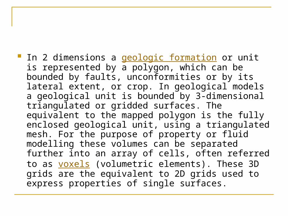
In 2 dimensions a geologic formation or unit is represented by a polygon, which can be bounded by faults, unconformities or by its lateral extent, or crop. In geological models a geological unit is bounded by 3-dimensional triangulated or gridded surfaces. The equivalent to the mapped polygon is the fully enclosed geological unit, using a triangulated mesh. For the purpose of property or fluid modelling these volumes can be separated further into an array of cells, often referred to as voxels (volumetric elements). These 3D grids are the equivalent to 2D grids used to express properties of single surfaces.

Videos

Geomodelling inputs

Geostatistics

Geostatistics is a branch of statistics focusing on spatial or spatiotemporal datasets. Developed originally to predict probability distributions of ore grades for mining operations, it is currently applied in diverse disciplines including petroleum geology, hydrogeology, hydrology, meteorology, oceanography, geochemistry, geometallurgy, geography, forestry, environmental control, landscape ecology, soil science, and agriculture (esp. in precision farming). Geostatistics is applied in varied branches of geography, particularly those involving the spread of diseases (epidemiology), the practice of commerce and military planning (logistics), and the development of efficient spatial networks. Geostatistical algorithms are incorporated in many places, including geographic information systems (GIS) and the R statistical environment.

Videos: Geostatics

Videos: Structural modelling

Stratigraphic modelling

Stratigraphic modelling has been long recognised as a method of presenting an organised picture of the unseen subterranean world. This has distinct advantages when trying to assess:

i. the extent of a resource (eg. oil, minerals, sand/aggregate, heavy minerals, groundwater);ii. geotechnical properties or;iii. environmental properties (eg. examine the spread of pollutants or potential pollutants).

Stratigraphy

Stratigraphy is a branch of geology which studies rock layers and layering (stratification). It is primarily used in the study of sedimentary and layered volcanic rocks. Stratigraphy includes two related subfields: lithologic stratigraphy or lithostratigraphy, and biologic stratigraphy or biostratigraphy.

Video: Stratigraphic modelling

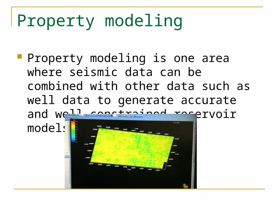
Property modeling

Property modeling is one area where seismic data can be combined with other data such as well data to generate accurate and well-constrained reservoir models.

Property modelling

2D property models are simple interpolations of the zone averages at the wells. This results in a lot of detail in the well data not being used, and very poor models of the vertical variability in the reservoir. Only by modelling in 3D can the use of the well data be maximised. 3D models also allow for the easier integration of other diverse data types. (e.g. seismic attributes).

Property & heterogeneity modelling Property & heterogeneity modelling The next step is to model the properties important to the

reservoir description. A full rante of deterministic & stocastic modelling techniques are

available. The techniques used will depend on the data available & the project aims.

A simple approach would be simple 3D interpolation of reservoir petrophysics, conditioned to only well data.

A more advanced approach would be to first capture the large scale heterogeneity through facies modelling. After the reservoir architecture has been captured the smaller scale heterongeneity can be conditioned to this using a variety of petrophysical modelling techniques. 3D seismic attributes can also be used to guide the modelling.

Structural modelling

Generating a hight quality structural framework is an essential first step in the 3D modelling workflow.

An integral part of structural modelling in modeling software is the construction of a fault model. This fault model can then be used to build 3D grids which honour both reservoir volumes and connectivity.

Building a fault model

Why build a fault model?Building a fauld model is not an essential part of the

the modeling software 3D modelling workflow. There are however many reasons to consider the inclusion of a fault model:

Accurate volumes in faulted areas Correct communications in 3D grid. Very important

for any dynamic modelling. Improved stratigraphic modelling Generate fault segments (blocks) for further

modelling control Generate separation diagrams

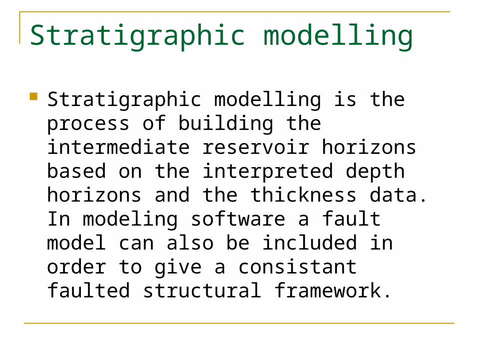
Stratigraphic modelling

Stratigraphic modelling is the process of building the intermediate reservoir horizons based on the interpreted depth horizons and the thickness data. In modeling software a fault model can also be included in order to give a consistant faulted structural framework.

Stratigraphic

Stratigraphic modelling is the process of building the intermediate reservoir horizons based on the interpreted depth horizons and thickness data. In modeling software a fault model can also be included in order to five a consistant faulted structural framework.

Terminology Interpreted horizon: A horizon derived from the seismic

interpretation. Can be time or depth. Must have an interpreted depth horizon for stratigraphic modelling. The horizons can be created from raw data in modeling software or can be imported.

Stratigraphic modelling is the process of building the intermediate reservoir horizons based on the interpreted depth horizons and thickness data. In modeling software a fault model can also be included in order to give a consistant faulted structural framework.

Stochastic Simulation

Stochastic simulation is a means for generating multiple equiprobable realizations of the property in question, rather than simply estimating the mean. Essentially, we are adding back in some noise to undo the smoothing effect of kriging. This possibly gives a better representation of the natural variability of the property in question and gives us a means for quantifying our uncertainty regarding what’s really down there. The two most commonly used forms of simulation for reservoir modeling applications are sequential Gaussian simulation for continuous variables like porosity and sequential indicator simulation for categorical variables like facies.The basic idea of sequential Gaussian simulation (SGS) is very simple. Recall that kriging gives us an estimate of both the mean and standard deviation of the variable at each grid node, meaning we can represent the variable at each grid node as a random variable following a normal (Gaussian) distribution. Rather than chooses the mean as the estimate at each node, SGS chooses a random deviate from this normal distribution, selected according to a uniform random number representing the probability level.

So, the basic steps in the SGS process are: Generate a random path through the grid nodes Visit the first node along the path and use kriging to estimate a mean and standard

deviation for the variable at that node based on surrounding data values Select a value at random from the corresponding normal distribution and set the

variable value at that node to that number Visit each successive node in the random path and repeat the process, including

previously simulated nodes as data values in the kriging process We use a random path to avoid artifacts induced by walking through the grid in a

regular fashion. We include previously simulated grid nodes as “data” in order to preserve the proper covariance structure between the simulated values.

Sometimes SGS is implemented in a “multigrid” fashion, first simulating on a coarse grid (a subset of the fine grid – maybe every 10 th grid node) and then on the finer grid (maybe with an intermediate step or two) in order to reproduce large-scale semivariogram structures. Without this the “screening” effect of kriging quickly takes over as the simulation progresses and nodes get filled in, so that most nodes are conditioned only on nearby values, so that small-scale structure is reproduced better than largescale structure.

Typical Reservoir Modeling Workflow Basically, work from large-scale structure to small-scale structure, and

generally from more deterministic methods to more stochastic methods: Establish large-scale geologic structure, for example, by deterministic

interpolation of formation tops; this creates a sete of distinct zones Within each zone, use SIS or some other discrete simulation technique (such

as object-based simulation) to generate realizations of the facies distribution – the primary control on the porosity & permeability distributions

Within each facies, use SGS (or similar) to generate porosity distirubtion and then simulate permeability distribution conditional to porosity distribution, assuming there is some relationship between the two Porosity and facies simulations could be conditioned to other secondary data, such as seismic. Methods also exist for conditioning to well test and production data, but these are fairly elaborate and probably not in very common use as yet. More typical (maybe) to run flow simulations after the fact and rank realizations by comparison to historical production & well tests.

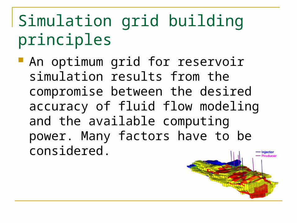
Simulation grid building principles An optimum grid for reservoir simulation

results from the compromise between the desired accuracy of fluid flow modeling and the available computing power. Many factors have to be considered.

Optimized grid size

The final number of grid blocks is often dictated by the available computing power. A few hundred thousand blocks for black oil and only a few then thousand blocks for compositional simulation are standard. The grid block size must, however, allow a minimum number of grid blocks between wells, remain within the correlation length of hereogeneities if multi-phase upscaling is to be avoided, as well as maintain acceptable levels of numerical dispersion. For the best compromise, grid blocks should be fine in high flow areas (near wells, in high permeability regions, etc) and coarse elsewhere (eg below OWC)

Flow-based orientation

Most reservoir simulators represent permeability as a diagonal tensor whose principal directions are parallel to the grid block`s median axes. Grids must therefore align with the main flow directions to avoid neglecting cross-flow. Faults, geological bodies (eg shale barriers), anisotropy and layering control the direction of flow. These should be reflected by the grid orientation. Ideally, layers should be parallel in the fine and the coarse grid. However, pinchouts increase simulation time.

Hierarchical fault incorporation Faults are key factors to reservoir connectivity.

Incorporating them in a grid generates many non-neighbour connections which slow down the simulation. Their inclusion must be decided upon their length, displacement, influence on flow as well as grid orientation. Major faults can define the grid frame, while secondary faults may be incorporated in such a way that the hexahedral shape required by corner-point geometry is preserved.

Corner point geometry

Grid blocks in corner point geometry can have their eight corners individually specified as long as they lie on straight (possibly sloping) co-ordinate lines joining the top and the bottom of the grid. This flexibility allows curvlinear grids but may result in skewed grids and inaccurate flow calculations as seen in figure 2.4. Cell distortion therefore needs to be carefully controlled.

Upscaling of heterogeneity

Upscaling is the process of assigning coarse simulation grid properties from the knowledge of small-scale geological properties. An upscaled of homogenized coarse grid value represents the effective property of the corresponding heterogenous volume.

Flow-based methods implement the following basic rule: find the permeability of the homogeneous medium that gives the same flux as the heterogenous medium under the same boundary conditions. Figure 4.2 shows the principle of the numerical experiment repeated for each simulation grid block and each direction: Apply a pressure drop and numerical boundary conditions Simulate fluid flow in the heterogenous volume Sum the flux accross the system Apply Darcy`s law to derive the effective permeability from

the total flux and the pressure drop Assign the effective permeability to the coarse grid block

Analytical methods like the arithmetic-harmonic and harmonic-arithmetic averages can sometimes approximate the result from the flow-based methods, but in the general case, they cannot reach the same accuracy.

Defining the re-scaling process In modeling software , re-scaling designates

the process of copying a parameter from a 3D grid into another using appropriate sampling and, if necessary, homogenisation methods. Here, we deal with upscaling, where the target (output) grid is normally coarser than the source (input) grid, and averaging methods should be carefully selected.

Upscaling is performed from a finely gridded 3D representation of the geological model into a coarser 3D grid covering roughly the same volume. Fine cells contributing to each coarse block are determined by various sampling methods which have to be chosen after considering the alignment between the two corner-point grids. Upscaling is then performed sequentially on every coarse grid block.

The upscaling process can be composed of several upscalers or re-scalers is defined by a fine-scale parameter, an upscaling method and various attributes for sampling options and method-specific settings.

Weight parameter

Simple averaging methods, summation and discrete methods allow using a weight parameter. Drop any fine grid parameter to use for weigthing into the drop site. Use this for rock or pore volume weigting.

For the discrete method, the weights are added and the rock type obtaining the highest sum is assigned to the coarse block.

Sampling method

The sampling method determines how the fine computation grid is built and populated with geological parameters. This is an essential pre-processing step to the upscaling.

Direct sampling

This is the default method. The fine grid from which effective properties are derived is made from the geological grid blocks hving their centre inside the simulation grid block, as pictured in figure 4.11. This respects the resolution and orientation of the geological grid. Cells are either counted all in or all out, unless `Use volume fractions` is toggled on (available only for simple methods).

Figure 4.12 shows how volume fractions can produce more accurate results for volumes.

Re-sampling. The fine grid used to derive effective properties is a uniform sub-division of the simulation grid block. This is faster to compute but may not match the fine grid resolution and orientation. Figure 4.13 shows the principle.

Reservoir simulation videos

Defining and calculating resources Defining and calculating resources and reservesand reserves

The total oil and gas estimated to have originally existed in the earth’s crust in naturally occurring accumulations is defined as original resources.

Original resources comprise discovered and undiscovered resources; in each of these, some are recoverable and some are unrecoverable.

The discovered recoverable resources are referred to as ultimate reserves — cumulative production plus future production (reserves).

The discovered unrecoverable resources are divided into contingent resources, which are technically recoverable but not economic, and unrecoverable resources, which are neither technically recoverable nor economic.

The undiscovered future recoverable resources are simply future production and are referred to as prospective resources, which are technically recoverable and economic. The undiscovered unrecoverable resources are neither technically recoverable nor economic

Discovered & undiscovered Discovered & undiscovered resourcesresources

Definitions of ResourcesDefinitions of Resources

Original ResourcesOriginal Resources

Original resources are those quantities of oil and gas estimated to exist originally in naturally occurring accumulations. They are, therefore, those quantities estimated on a given date to be remaining in known accumulations plus those quantities already produced from known accumulations plus those quantities in accumulations yet to be discovered. Original resources are divided into discovered and undiscovered resources, with discovered resources limited to known accumulations.

Discovered ResourcesDiscovered Resources

Discovered resources are those quantities of oil and gas estimated on a given date to be remaining in, plus those quantities already produced from, known accumulations.

Discovered resources are divided into economic and uneconomic categories, with the estimated future recoverable portion classified as reserves and contingent resources, respectively.

ReservesReserves

Those quantities of oil and gas anticipated to be economically recoverable from discovered resources are classified as reserves

Estimated recoverable quantities from known accumulations that are not economic are classified as contingent resources. The definition of economic for an accumulation will vary according to local conditions of prices, costs, and operating circumstances and is left to the discretion of the country or company concerned.

Nevertheless, reserves must be classified according to the definitions. In general, quantities must not be classified as reserves unless there is an expectation that the accumulation will be developed and placed on production within a reasonable timeframe.

In certain circumstances, reserves can be assigned to known accumulations even though development might not occur for some time. For example, fields might be dedicated to a long-term supply contract and will only be developed when they are needed to satisfy that contract.

Contingent ResourcesContingent Resources

Contingent resources are defined as those quantities of oil and gas estimated on a given date to be potentially recoverable from known accumulations but are not currently economic. Contingent resources include, for example, accumulations for which there is currently no viable market.

Undiscovered resources are defined as those quantities of oil and gas estimated on a given date to be contained in accumulations yet to be discovered. The estimated potentially recoverable portion of undiscovered resources is classified as prospective resources.

Prospective resources are defined as those quantities of oil and gas estimated on a given date to be potentially recoverable from undiscovered accumulations. They are technically viable and economic to recover.

Discovered and Undiscovered Unrecoverable Resources Unrecoverable resources, whether discovered or undiscovered,

are neither technically possible nor economic to produce. They represent quantities of petroleum that are in the reservoir after commercial production has ceased, and in known and unknown accumulations that are not deemed recoverable due to lack of technical and economic recovery processes.

Resources Categories Due to the high uncertainty in estimating resources, evaluations

of these assets require some type of probabilistic method. Expected value concepts and decision tree analyses are routine; however, in high-risk, high-reward projects, Monte Carlo simulation can be used. In any event, three success cases plus a failure case should be included in the evaluation of the resources.

Classification of Resources When evaluating resources, in particular contingent and prospective

resources, the following mutually exclusive categories are recommended: Low Estimate: This is considered to be a conservative estimate of the

quantity that will actually be recovered from the accumulation. If probabilistic methods are used, this term reflects a P90 confidence level.

Best Estimate: This is considered to be the best estimate of the quantity that will actually be recovered from the accumulation. If probabilistic methods are used, this term is a measure of central tendency of the uncertainty distribution (most likely/mode, P50/median, or arithmetic average/mean.)

High Estimate: This is considered to be an optimistic estimate of the quantity that will actually be recovered from the accumulation. If probabilistic methods are used, this term reflects a P10 confidence level.

Definitions of ReservesDefinitions of Reserves

Reserves Categories Reserves are estimated remaining quantities of oil and natural gas and

related substances anticipated to be recoverable from known accumulations, from a given date forward, based on analysis of drilling, geological, geophysical, and engineering data; the use of established technology; specified economic conditions, which are generally accepted as being reasonable, and shall

be disclosed. Reserves are classified according to the degree of certainty associated with

the estimates Proved Reserves Proved reserves are those reserves that can be estimated with a high

degree of certainty to be recoverable. It is likely that the actual remaining quantities recovered will exceed the estimated proved reserves.

Probable Reserves Probable reserves are those additional reserves that are less certain to be

recovered than proved reserves. It is equally likely that the actual remaining quantities recovered will be greater or less than the sum of the estimated proved + probable reserves.

Possible Reserve Possible reserves are those additional reserves that are less certain to be

recovered than probable reserves. It is unlikely that the actual remaining quantities recovered will exceed the sum of the estimated proved + probable + possible reserves.

Development and Production StatusDevelopment and Production Status Each of the reserves categories (proved, probable, and possible) may be

divided into developed and undeveloped categories. Developed Reserves Developed reserves are those reserves that are expected to be recovered

from existing wells and installed facilities or, if facilities have not been installed, that would involve a low expenditure (e.g., when compared to the cost of drilling a well) to put the reserves on production. The developed category may be subdivided into producing and non-producing.

Developed Producing Reserves Developed producing reserves are those reserves that are expected to be

recovered from completion intervals open at the time of the estimate. These reserves may be currently producing or, if shut in, they must have previously been on production, and the date of resumption of production must be known with reasonable certainty.

Developed Non-Producing Reserves Developed non-producing reserves are those reserves that either have not been

on production, or have previously been on production, but are shut in, and the date of resumption of production is unknown.

Undeveloped Reserves Undeveloped reserves are those reserves expected to be recovered from

known accumulations where a significant expenditure (e.g., when compared to the cost of drilling a well) is required to render them capable of production. They must fully meet the requirements of the reserves classification (proved, probable, possible) to which they are assigned.

In multi-well pools, it may be appropriate to allocate total pool reserves between the developed and undeveloped categories or to subdivide the developed reserves for the pool between developed producing and developed non-producing. This allocation should be based on the estimator’s assessment as to the reserves that will be recovered from specific wells, facilities, and completion intervals in the pool and their respective development and production status.

Levels of Certainty for Reported Reserves Reported Reserves should target the following levels of certainty under a specific set of economic conditions:

at least a 90 percent probability that the quantities actually recovered will equal or exceed the estimated proved reserves;

at least a 50 percent probability that the quantities actually recovered will equal or exceed the sum of the estimated proved + probable reserves;

at least a 10 percent probability that the quantities actually recovered will equal or exceed the sum of the estimated proved + probable + possible reserves.

A quantitative measure of the certainty levels pertaining to estimates prepared for the various reserves categories is desirable to provide a clearer understanding of the associated risks and uncertainties. However, the majority of reserves estimates will be prepared using deterministic methods that do not provide a mathematically derived quantitative measure of probability. In principle, there should be no difference between estimates prepared using probabilistic or deterministic methods.

General Guidelines for Estimation General Guidelines for Estimation of Reservesof Reserves Uncertainty in Reserves Estimation Reserves estimation has characteristics that are common to any measurement

process that uses uncertain data. An understanding of statistical concepts and the associated terminology is essential to understanding the confidence associated with reserves definitions and categories.

Uncertainty in a reserves estimate arises from a combination of error and bias: Error is inherent in the data that are used to estimate reserves. Note that the term “error” refers to

limitations in the input data, not to a mistake in interpretation or application of the data. The procedures and concepts dealing with error lie within the realm of statistics and are well established.

Bias, which is a predisposition of the evaluator, has various sources that are not necessarily conscious or intentional.

In the absence of bias, different qualified evaluators using the same information at the same time should produce reserves estimates that will not be materially different, particularly for the aggregate of a large number of estimates. The range within which these estimates should reasonably fall depends on the quantity and quality of the basic information, and the extent of analysis of the data

Deterministic and Probabilistic Method Reserves estimates may be prepared using either deterministic or probabilistic

methods. Deterministic Method The deterministic approach, which is the one most commonly employed

worldwide, involves the selection of a single value for each parameter in the reserves calculation. The discrete value for each parameter is selected based on the estimator’s determination of the value that is most appropriate for the corresponding reserves category.

Probabilistic Method Probabilistic analysis involves describing the full range of possible values for

each unknown parameter. This approach typically consists of employing computer software to perform repetitive calculations (e.g., Monte Carlo simulation) to generate the full range of possible outcomes and their associated probability of occurrence.

Comparison of Deterministic and Probabilistic Estimates Deterministic and probabilistic methods are not distinct and separate. A

deterministic estimate is a single value within a range of outcomes that could be derived by a probabilistic analysis. There should be no material difference between Reported Reserves estimates prepared using deterministic and probabilistic methods.

Application of Guidelines to the Probabilistic Method The following guidelines include criteria that provide specific limits to

parameters for proved reserves estimates. For example, volumetric estimates are restricted by the lowest known hydrocarbon (LKH). Inclusion of such specific limits may conflict with standard probabilistic procedures, which require that input parameters honour the range of potential values.

Nonetheless, it is required that the guidelines be met regardless of analysis method. Accordingly, when probabilistic methods are used, constraints on input parameters may be required in certain instances. Alternatively, a deterministic check may be made in such instances to ensure that aggregate estimates prepared using probabilistic methods do not exceed those prepared using a deterministic approach including all appropriate constraints.

General Requirements for General Requirements for Classification of ReservesClassification of Reserves Drilling Requirements Proved, probable, or possible reserves may be assigned only to known

accumulations that have been penetrated by a wellbore. Potential hydrocarbon accumulations that have not been penetrated by a wellbore may be classified as prospective resources.

Testing Requirements Confirmation of commercial productivity of an accumulation by production or

a formation test is required for classification of reserves as proved. In the absence of production or formation testing, probable and/or possible reserves may be assigned to an accumulation on the basis of well logs and/or core analysis that indicate that the zone is hydrocarbon bearing and is analogous to other reservoirs in the immediate area that have demonstrated commercial productivity by actual production or formation testing.

Economic Requirements Proved, probable, or possible reserves may be assigned only to

those volumes that are economically recoverable. The fiscal conditions under which reserves estimates are prepared should generally be those which are considered to be a reasonable outlook on the future. If required by securities regulators or other agencies, constant or other prices and costs also may be used. In any event, the fiscal assumptions used in the preparation of reserves estimates must be disclosed.

Undeveloped recoverable volumes must have a sufficient return on investment to justify the associated capital expenditure in order to be classified as reserves, as opposed to contingent resources.

Regulatory Considerations In general, proved, probable, or possible reserves may be assigned

only in instances where production or development of those reserves is not prohibited by governmental regulation. This provision would, for instance, preclude the assignment of reserves in designated environmentally sensitive areas. Reserves may be assigned in instances where regulatory restraints may be removed subject to satisfaction of minor conditions. In such cases, the classification of reserves as proved, probable, or possible should be made with consideration given to the risk associated with project approval.

Procedures for Estimation and Procedures for Estimation and Classification of ReservesClassification of Reserves

The process of reserves estimation falls into three broad categories: volumetric material balance, and decline analysis. Selection of the most appropriate reserves estimation procedures depends on the information that is available. Generally, the range of uncertainty associated with an estimate decreases and confidence level increases as more information becomes available, and when the estimate is supported by more than one estimation method.

Volumetric Methods Volumetric methods involve the calculation of reservoir rock volume,

the hydrocarbons in place in that rock volume, and the estimation of the portion of the hydrocarbons in place that ultimately will be recovered. For various reservoir types at varied stages of development and depletion, the key unknown in volumetric reserves determinations may be rock volume, effective porosity, fluid saturation, or recovery factor. Important considerations affecting a volumetric reserves estimate are outlined below:

Rock Volume: Rock volume may simply be determined as the product of a single well drainage area and wellbore net pay or by more complex geological mapping. Estimates must take into account geological characteristics, reservoir fluid properties, and the drainage area that could be expected from the well or wells. Consideration must be given to any limitations indicated by geological, geophysical data or interpretations, as well as pressure depletion or boundary conditions exhibited by test data.

Elevation of Fluid Contacts: In the absence of data that clearly define fluid contacts, the structural interval for volumetric calculations of proved reserves should be restricted by the lowest known structural elevation of occurrence of hydrocarbons (LKH) as defined by well logs, core analyses, or formation testing.

Effective Porosity, Fluid Saturation and Other Reservoir Parameters: These are determined from logs and core and well test data.

Recovery Factor: Recovery factor is based on analysis of production behaviour from the subject reservoir, by analogy with other producing reservoirs and/or by engineering analysis. In estimating recovery factors, the evaluator must consider factors that influence recoveries, such as rock and fluid properties, hydrocarbons in place, drilling density, future changes in operating conditions, depletion mechanisms, and economic factors.

Material Balance Methods Material balance methods of reserves estimation involve the

analysis of pressure behaviour as reservoir fluids are withdrawn, and generally result in more reliable reserves estimates than volumetric estimates. Reserves may be based on material balance calculations when sufficient production and pressure data are available.

Confident application of material balance methods requires knowledge of rock and fluid properties, aquifer characteristics, and accurate average reservoir pressures. In complex situations, such as those involving water influx, multi-phase behaviour, multi-layered, or low permeability reservoirs, material balance estimates alone may provide erroneous results.

Computer reservoir modeling can be considered a sophisticated form of material balance analysis. While modeling can be a reliable predictor of reservoir behaviour, the input rock properties, reservoir geometry, and fluid properties are critical.

Evaluators must be aware of the limitations of predictive models when using these results for reserves estimation.

The portion of reserves estimated as proved, probable, or possible should reflect the quantity and quality of the available data and the confidence in the associated estimate.

Production Decline Method

Production decline analysis methods of reserves estimation involve

the analysis of production behaviour as reservoir fluids are

withdrawn. Confident application of decline analysis methods

requires a sufficient period of stable operating conditions after the

wells in a reservoir have established drainage areas. In estimating

reserves, evaluators must take into consideration factors affecting

production decline behaviour, such as reservoir rock and fluid

properties, transient versus stabilized flow, changes in operating

conditions (both past and future), and depletion mechanism.

Reserves may be assigned based on decline analysis when sufficient production data are available. The decline relationship used in projecting production should be supported by all available data. The portion of reserves estimated as proved, probable, or possible should reflect the confidence in the associated estimate.

Future Drilling and Planned Enhanced Recovery Projects The foregoing reserves estimation methodologies are

applicable to recoveries from existing wells and enhanced recovery projects that have been demonstrated to be economically and technically successful in the subject reservoir by actual performance or a successful pilot. The following criteria should be considered when estimating incremental reserves associated with development drilling or implementation of enhanced recovery projects. In all instances, the probability of recovery of the associated reserves must meet the certainty criteria contained in previous section.

Additional Reserves Related to Future Drilling Additional reserves associated with future drilling in known

accumulations may be assigned where economics support and regulations do not prohibit the drilling of the location.

Aside from the criteria stipulated in previous section, factors to be considered in classifying reserves estimates associated with future drilling as proved, probable, or possible include whether the proposed location directly offsets existing wells or acreage

with proved or probable reserves assigned, the expected degree of geological continuity within the reservoir unit

containing the reserves, the likelihood that the location will be drilled

In addition, where infill wells will be drilled and placed on production, the evaluator must quantify well interference effects, that portion of infill well recovery that represents accelerated production of developed reserves, and that portion that represents incremental recovery beyond those reserves recognized for the existing reservoir development.

Reserves Related to Planned Enhanced Recovery Projects Reserves that can be economically recovered through the future

application of an established enhanced recovery method may be classified as follows.

Proved reserves may be assigned to planned enhanced recovery projects when the following criteria are met: Repeated commercial success of the enhanced recovery process has been

demonstrated in reservoirs in the area with analogous rock and fluid properties.

The project is highly likely to be carried out in the near future. This may be demonstrated by factors such as the commitment of project funding.

Where required, either regulatory approvals have been obtained, or no regulatory impediments are expected, as clearly demonstrated by the approval of analogous projects.

Probable reserves may be assigned when a planned enhanced recovery project does not meet the requirements for classification as proved; however, the following criteria are met: The project can be shown to be practically and technically reasonable. Commercial success of the enhanced recovery process has been demonstrated in

reservoirs with analogous rock and fluid properties. It is reasonably certain that the project will be implemented.

Possible reserves may be assigned when a planned enhanced recovery project does not meet the requirements for classification as proved or probable; however, the following criteria are met: The project can be shown to be practically and technically reasonable. Commercial success of the enhanced recovery process has been demonstrated in

reservoirs with analogous rock and fluid properties, but there remains some doubt that the process will be successful in the subject reservoir.

Validation of Reserves Estimate A practical method of validating and confirming that reserves estimates

meet the definitions and guidelines is through periodic reserves reconciliation of both entity and aggregate estimates. The tests described below should be applied to the same entities or groups of entities over time, excluding revisions due to differing economic assumptions: Revisions to proved reserves estimates should generally be positive as new

information becomes available. Revisions to proved + probable reserves estimates should generally be neutral as new

information becomes available. Revisions to proved + probable + possible estimates should generally be negative as

new information becomes available. These tests can be used to monitor whether procedures and practices employed are

achieving results consistent with certainty criteria contained in previous section. In the event that the above tests are not satisfied on a consistent basis, appropriate adjustments should be made to evaluation procedures and practices.

Reservoir modeling and characterization

Engineering

Transcript of Reservoir modeling and characterization