71

CHAPTER – V

DEVELOPMENT OF ANN MODEL

5.0 ARTIFICIAL NEURAL NETWORK (ANN)

Either from known or unknown source, a neural network may be

trained with measured data. There are software tools designed to

estimate the relationships in data where they can be trained to perform

classification, estimation, simulation and prediction of the underlying

process generating the data. The Neural Networks package supports

several function estimation techniques that may be described in terms of

the different types of neural networks and associated learning

algorithms. Artificial neural networks are nonlinear information (signal)

processing devices, which are built from interconnected elementary

processing devices called neurons. ANN is a very important tool for

studying the structure-function relationship of the human brain. Each

computing unit, i.e, the artificial neuron in the neural network is based

on the concept of an ideal neuron. An Artificial Neural Network (ANN) is

an information-processing paradigm that is inspired by the way of

biological nervous systems, such as brain and process information. It is

composed of a large number of highly interconnected processing

elements (neurons) working in union to solve specific problems. Since

most manufacturing processes are complex in nature, highly non-linear,

72

and there are a large number of input variables, there is no accurate

mathematical model which can describe the behavior of these processes.

A neural network is a massively parallel-distributed processor that

has a natural propensity for storing experimental knowledge and making

it available for use. Knowledge is acquired by the network through a

learning process, and Inter-neuron connection strengths known as

synaptic weights are used to store the knowledge.

Much research is related to applications of Artificial Intelligence

(AI), especially Artificial Neural Networks (ANN), for engineering fields

such as manufacturing processes prediction, monitoring and controlling.

Thus, the new approach which ensures efficient and fast selection of the

optimum conditions and processing of available technological data are

the ANNs and they are mostly used in the fields of biology, electronics,

computer science, mathematics and engineering. The method has proved

to be excellent for solving the optimization problems, for pattern

recognition and for the adaptive control of machines.

5.1 BUILDING BLOCKS OF ARTIFICAL NEURAL NETWORK

The basic building blocks of the artificial neural network are

1. Network architecture

2. Setting the weights

3. Activation function

73

5.1.1 Network Architecture

The arrangement of neurons into layers and the pattern of connection

within and in between the layers is generally called as the architecture of

the network. Feed forward, feedback, fully interconnected network,

competitive network, etc. are the various types of network architectures.

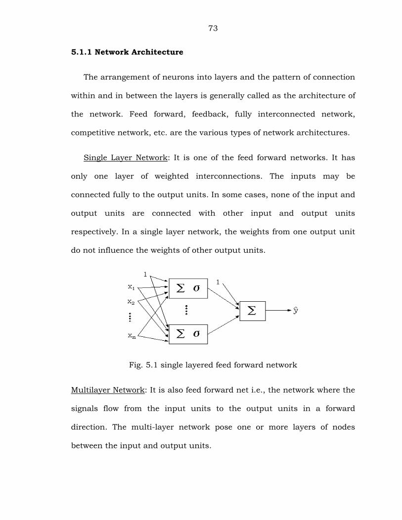
Single Layer Network: It is one of the feed forward networks. It has

only one layer of weighted interconnections. The inputs may be

connected fully to the output units. In some cases, none of the input and

output units are connected with other input and output units

respectively. In a single layer network, the weights from one output unit

do not influence the weights of other output units.

Fig. 5.1 single layered feed forward network

Multilayer Network: It is also feed forward net i.e., the network where the

signals flow from the input units to the output units in a forward

direction. The multi-layer network pose one or more layers of nodes

between the input and output units.

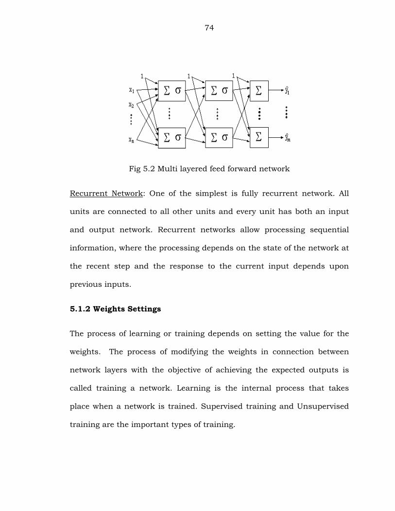
74

Fig 5.2 Multi layered feed forward network

Recurrent Network: One of the simplest is fully recurrent network. All

units are connected to all other units and every unit has both an input

and output network. Recurrent networks allow processing sequential

information, where the processing depends on the state of the network at

the recent step and the response to the current input depends upon

previous inputs.

5.1.2 Weights Settings

The process of learning or training depends on setting the value for the

weights. The process of modifying the weights in connection between

network layers with the objective of achieving the expected outputs is

called training a network. Learning is the internal process that takes

place when a network is trained. Supervised training and Unsupervised

training are the important types of training.

75

Supervised Training: Supervised training is the process of providing the

network with a series of sample inputs and comparing the outputs with

the expected responses. The training continues until the network is able

to provide the expected response. In a neural network, for a sequence of

training inputs there exist target output vectors. The weights may then

be adjusted according to a learning algorithm. This process is called

supervised training.

Unsupervised Training: If the output is unknown, for the training input

vectors the method of unsupervised training is used. The network may

modify the weight so that the most similar input vector is assigned to a

same output unit. It is expected to form an example or code book vector

for each cluster formed.

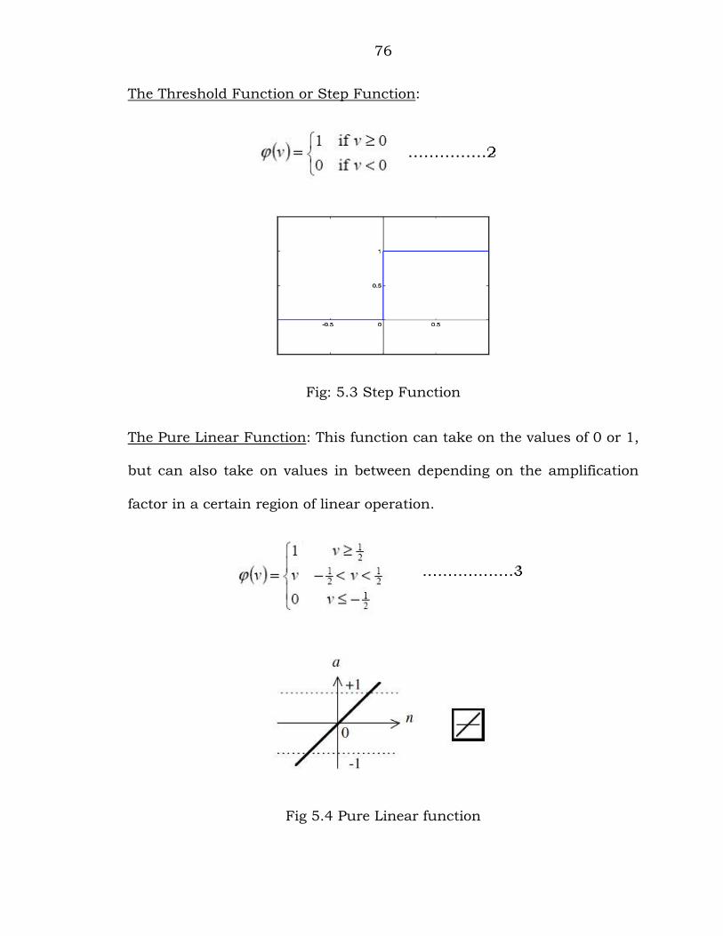
5.1.3 Activation Function

The activation function is used to calculate the output response of

neuron. The sum of the weighted input signal is applied with an

activation to obtain the response. Same activation functions are used for

neurons in the same layer. The non-linear activation functions are used

in a multilayer network. The output of a neuron in a neural network is

between certain values (usually 0 and 1, or -1 and 1). In general, there

are three types of activation functions they are the threshold function or

step function, the pure linear function and sigmoid function.

76

The Threshold Function or Step Function:

Fig: 5.3 Step Function

The Pure Linear Function: This function can take on the values of 0 or 1,

but can also take on values in between depending on the amplification

factor in a certain region of linear operation.

Fig 5.4 Pure Linear function

77

The Sigmoid Function: This function can range between 0 and 1. This

function is generally used in multi-layered networks that are trained

using back propagation algorithm.

Fig 5.5 Log-Sigmoid Function

5.2 LEARNING RULES

The process by which the free parameters of a neural network get

adapted through a process of stimulating by the environment in which

the network is embedded is learning.

5.2.1 HEBBIAN LEARNING RULE

Hebb’s learning says that, if two neurons on either side of a synapse

are activated simultaneously, then the strength of the synapse is

selectively increased and activated asynchronously, then that synapse is

selectively weakened or eliminated. If the cross product of output and

78

input is positive, this result in increase of weight, otherwise the weight

decreases.

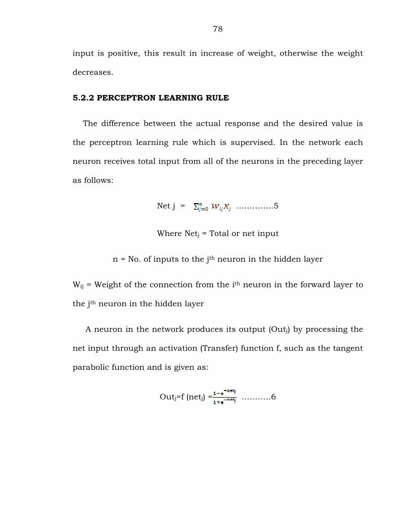
5.2.2 PERCEPTRON LEARNING RULE

The difference between the actual response and the desired value is

the perceptron learning rule which is supervised. In the network each

neuron receives total input from all of the neurons in the preceding layer

as follows:

Net j = …………..5

Where Netj = Total or net input

n = No. of inputs to the jth neuron in the hidden layer

Wij = Weight of the connection from the ith neuron in the forward layer to

the jth neuron in the hidden layer

A neuron in the network produces its output (Outj) by processing the

net input through an activation (Transfer) function f, such as the tangent

parabolic function and is given as:

Outj=f (netj) = ..………6

79

5.2.3 DELTA LEARNING RULE or LEAST MEAN SQUARE RULE (LMS)

The delta learning rule, a supervised learning rule is valid only for

continuous activation functions. The learning signal for this rule is called

delta. The aim of the delta rule is to minimize the error in the overall

training patterns.

5.2.4 COMPETITIVE LEARNING RULE

The idea behind this rule is that there are a set of neurons that are

similar in all aspects except for some randomly distributed synaptic

weights, and hence are expected to respond differently to a given set of

input patterns. This rule has a mechanism such that only one output

neuron or only one neuron per group is active at a time. The rule is

suited for unsupervised network training.

N=1 if Vp>Vq for all q, p=q

=0 otherwise …………7

5.2.5 BOLTZMAN LEARNING

This is a stochastic learning. A neural net designed based on this

learning is called Boltzmann learning. This learning is characterized by

an energy function, E, the value of which is determined by the particular

states occupied by the individual neurons of the machine, given by

80

………..8

Where Xi is the state of neuron i, and Wij is the weight from neuron i to

neuron j. The operation of machine is performed by choosing a neuron

at random.

5.3 MATLAB SOFTWARE

MATLAB (matrix laboratory) is a high-level language with interactive

environment that enables to perform computationally intensive tasks

faster than with traditional programming languages such as C, C++ and

FORTRAN. In teaching linear algebra and numerical analysis, MATLAB is

used and has become a useful tool for problem solving in many areas.

The problems and solutions are expressed in mathematical notation.

Areas of application of MATLAB include

1) Maths and computation

2) Algorithm development

3) Modeling, simulation and prototyping

4) Data analysis, exploration and visualization

5) Scientific and engineering graphics

6) Application development, including graphical user interface

building.

81

5.3.1 Toolboxes

The various toolboxes available in MATLAB are Control system,

Communications, Signal processing, System Identification, Robust

Control, Simulink, Neural Network, Fuzzy Logic, Image Processing,

Analysis, Optimization, Spline and Symbolic

5.4 DEVELOPING NEURAL NETWORK

MATLAB platform is used for developing a Neural Network Model.

ANNs are computational models, which replicate the function of a

biological network, composed of neurons and are used to solve complex

functions in various applications. Neural networks are a non linear

mapping system that consists of simple processors, which are called

neurons linked by weighted connections. An output is generated with

each input neuron which is seen as the reflection that is stored in

connections [53, 55]. The output signal of a neuron is fed to the other

neurons through inter connections as input signals. If the function is

complex in nature, as the capability of single neuron is limited, many

processing elements are connected. The performance of the network

depends on the activation function, network structure, data

representation and normalization of inputs and outputs.

The measured tensile strength results are used to train, and two

networks are trained. Network1 and Network2 are created based on the

82

tool profiles. Network1 is for square pin profile tool and Network2 is for

modified square pin profile tool.

The network created is a two layered feed forward network by

considering TRS, WS and F as inputs and number of hidden layer is one.

Network1 and Network2 consists of two layers. Tangent sigmoid function

is the network transfer function, and the neural network model is trained

using Levenberg- Marquardt Algorithm.

The following are the steps for developing the network:

1. Database collection.

2. Analysis and pre-processing of the data.

3. Training of the neural network.

4. Test of the trained network.

5. Post processing of data.

6. Use of the trained NN for simulation and prediction.

5.5 ANN MODEL FOR SQUARE PROFILED TOOL

The experimental work is carried by varying the parameters, and

from the results obtained by conducting DOE and ANOVA, it can be

drawn that the mechanical properties obtained using square profiled tool

are better when compared to other tools. An ANN model is developed for

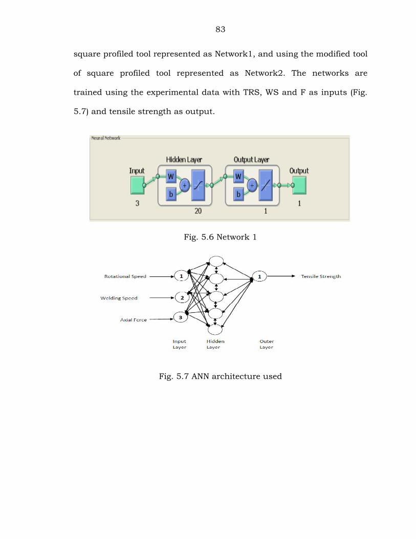
83

square profiled tool represented as Network1, and using the modified tool

of square profiled tool represented as Network2. The networks are

trained using the experimental data with TRS, WS and F as inputs (Fig.

5.7) and tensile strength as output.

Fig. 5.6 Network 1

Fig. 5.7 ANN architecture used

84

Fig.5.8 Training Parameters of Network1

In this work, the neural network is trained by using Levenberg -

Marquardt algorithm. The training parameters are shown below.

Fig. 5.9 Training Algorithm of Network1

85

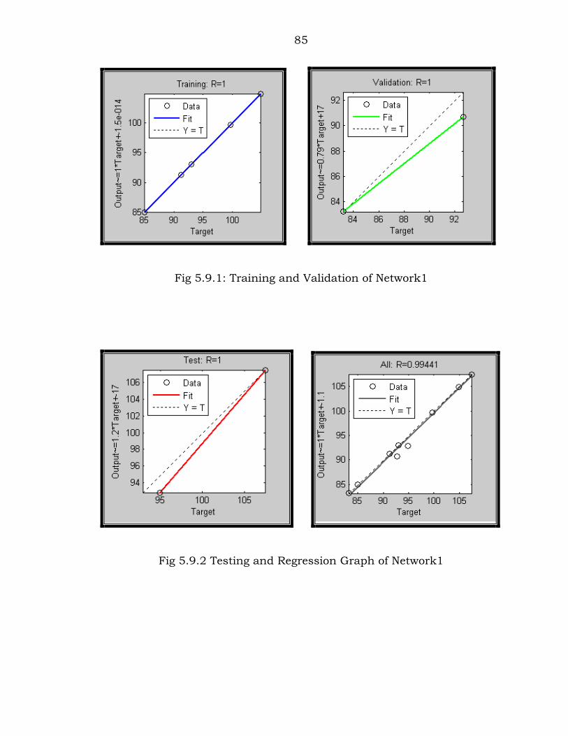
Fig 5.9.1: Training and Validation of Network1

Fig 5.9.2 Testing and Regression Graph of Network1

86

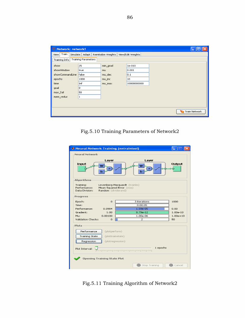
Fig.5.10 Training Parameters of Network2

Fig.5.11 Training Algorithm of Network2

87

Fig. 5.11.1 Training and Validation of Network2

Fig. 5.11.2: Testing and Regression of Network2