Artificial Neural NetworksArtificial Neural...
132
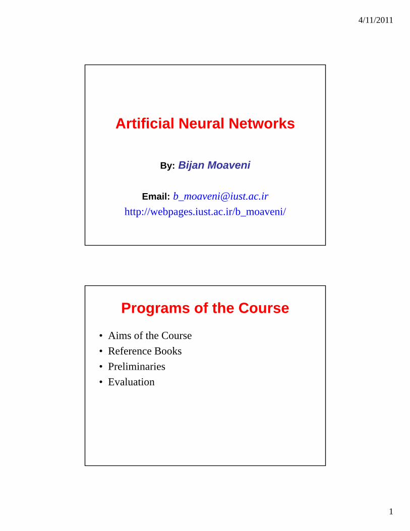
4/11/2011 1 Artificial Neural Networks Artificial Neural Networks By: Bijan Moaveni Email: [email protected] http://webpages.iust.ac.ir/b_moaveni/ Programs of the Course • Aims of the Course • Reference Books • Preliminaries • Evaluation
Transcript of Artificial Neural NetworksArtificial Neural...
4/11/2011
1
Artificial Neural NetworksArtificial Neural Networks
By: Bijan Moaveni
Email: [email protected]
http://webpages.iust.ac.ir/b_moaveni/
Programs of the Course
• Aims of the Course
• Reference Books
• Preliminaries
• Evaluation
4/11/2011
2
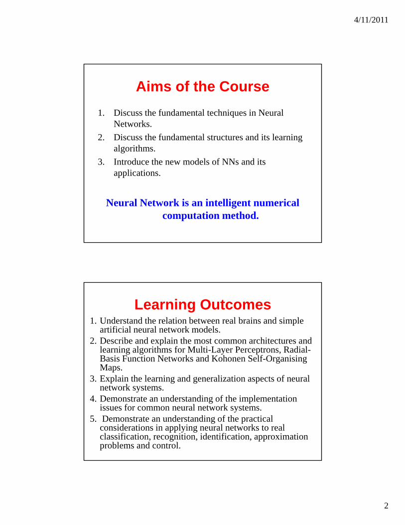
Aims of the Course
1. Discuss the fundamental techniques in Neural NetworksNetworks.
2. Discuss the fundamental structures and its learning algorithms.
3. Introduce the new models of NNs and its applications.
Neural Network is an intelligent numerical computation method.
Learning Outcomes1. Understand the relation between real brains and simple
artificial neural network models.2 Describe and explain the most common architectures and2. Describe and explain the most common architectures and
learning algorithms for Multi-Layer Perceptrons, Radial-Basis Function Networks and Kohonen Self-Organising Maps.
3. Explain the learning and generalization aspects of neural network systems.
4. Demonstrate an understanding of the implementation4. Demonstrate an understanding of the implementation issues for common neural network systems.
5. Demonstrate an understanding of the practical considerations in applying neural networks to real classification, recognition, identification, approximation problems and control.

4/11/2011
3
Course Evaluation
1. Course Projects 40%
2. Final Exam 50%
3. Conference Paper 10%
Reference Books
• Haykin S., Neural Networks: A Comprehensive P ti H ll 1999Foundation., Prentice Hall, 1999.
• Hagan M.T., Dcmuth H.B. and Beale M., Neural Network Design, PWS Publishing Co., 1996.
4/11/2011
4
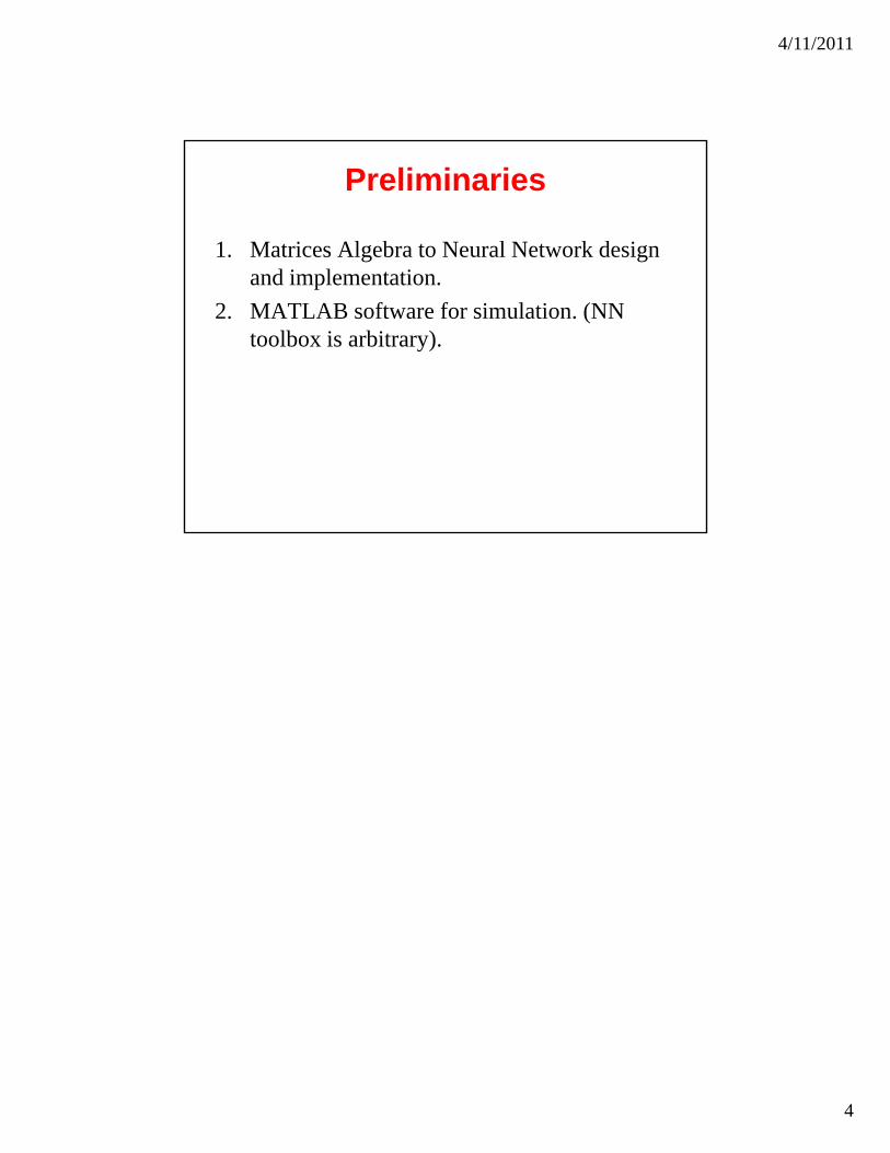
Preliminaries
1. Matrices Algebra to Neural Network design d i l t tiand implementation.
2. MATLAB software for simulation. (NN toolbox is arbitrary).
4/11/2011
1
Artificial Neural NetworksArtificial Neural Networks
Lecture 2
1
Introduction1. What are Neural Networks?2. Why are Artificial Neural Networks Worth2. Why are Artificial Neural Networks Worth
Noting and Studying?3. What are Artificial Neural Networks used for?4. Learning in Neural Networks5. A Brief History of the Field
2
6. Artificial Neural Networks compared with Classical Symbolic A.I.
7. Some Current Artificial Neural Network Applications
4/11/2011
2
What are Neural Networks?
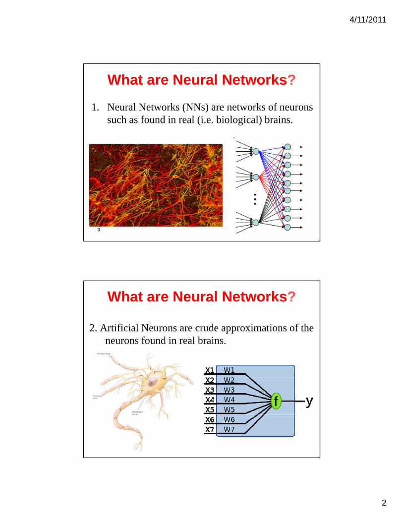
1. Neural Networks (NNs) are networks of neurons such as found in real (i.e. biological) brains.such as found in real (i.e. biological) brains.
3
What are Neural Networks?
2. Artificial Neurons are crude approximations of the neurons found in real brainsneurons found in real brains.
4
4/11/2011
3
What are Neural Networks?
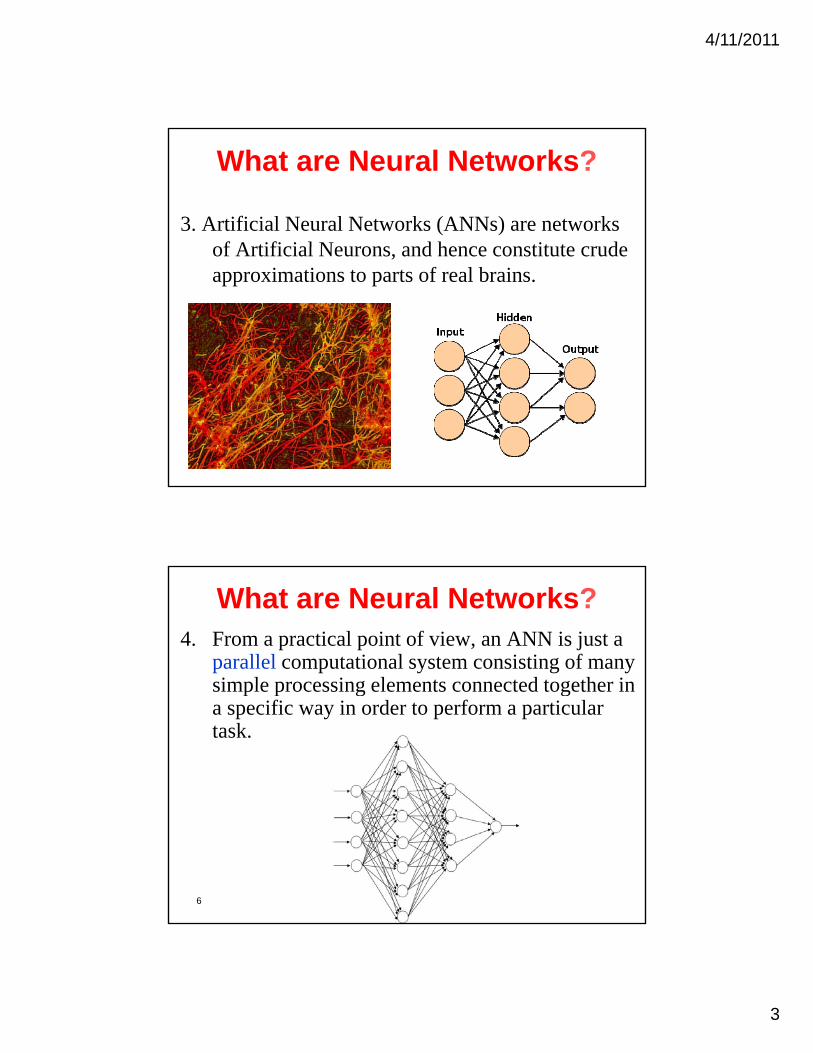
3. Artificial Neural Networks (ANNs) are networks of Artificial Neurons and hence constitute crudeof Artificial Neurons, and hence constitute crude approximations to parts of real brains.
5
What are Neural Networks?4. From a practical point of view, an ANN is just a
parallel computational system consisting of many simple processing elements connected together insimple processing elements connected together in a specific way in order to perform a particular task.
6
4/11/2011
4
Why are Artificial Neural Networks Worth Noting and Studying?
1. They are extremely powerful computational devices.
2 Parallel Processing makes them very efficient2. Parallel Processing makes them very efficient.
3. They can learn and generalize from training data – so there is no need for enormous feats of programming.
4. They are particularly fault tolerant – this is equivalent to the “graceful degradation” found in biological systems.
7
5. They are very noise tolerant – so they can cope or deal with situations where normal symbolic (classic) systems would have difficulty.
6. In principle, they can do anything a symbolic or classic system can do, and more.
What are Artificial Neural Networks used for?
• Brain modeling : The scientific goal of building models of how real brains work This canmodels of how real brains work. This can potentially help us understand the nature of human intelligence, formulate better teaching strategies, or better remedial actions for brain damaged patients.
• Artificial System Building : The engineering
8
Artificial System Building : The engineering goal of building efficient systems for real world applications. This may make machines more powerful, relieve humans of tedious tasks, and may even improve upon human performance.
4/11/2011
5
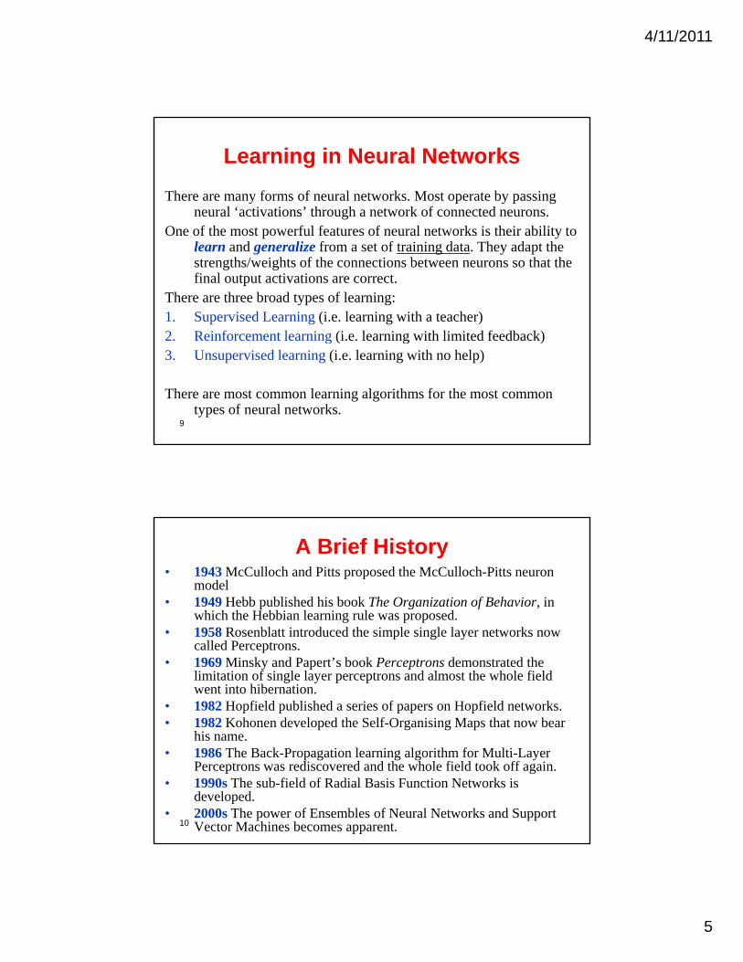
Learning in Neural Networks
There are many forms of neural networks. Most operate by passing neural ‘activations’ through a network of connected neurons.
O f h f l f f l k i h i biliOne of the most powerful features of neural networks is their ability to learn and generalize from a set of training data. They adapt the strengths/weights of the connections between neurons so that the final output activations are correct.
There are three broad types of learning:1. Supervised Learning (i.e. learning with a teacher)2 Reinforcement learning (i e learning with limited feedback)
9
2. Reinforcement learning (i.e. learning with limited feedback)3. Unsupervised learning (i.e. learning with no help)
There are most common learning algorithms for the most common types of neural networks.
A Brief History• 1943 McCulloch and Pitts proposed the McCulloch-Pitts neuron
model• 1949 Hebb published his book The Organization of Behavior, in
which the Hebbian learning rule was proposed.• 1958 Rosenblatt introduced the simple single layer networks now
called Perceptrons.• 1969 Minsky and Papert’s book Perceptrons demonstrated the
limitation of single layer perceptrons and almost the whole field went into hibernation.
• 1982 Hopfield published a series of papers on Hopfield networks.• 1982 Kohonen developed the Self-Organising Maps that now bear
his name
10
his name.• 1986 The Back-Propagation learning algorithm for Multi-Layer
Perceptrons was rediscovered and the whole field took off again.• 1990s The sub-field of Radial Basis Function Networks is
developed.• 2000s The power of Ensembles of Neural Networks and Support
Vector Machines becomes apparent.

4/11/2011
6
A Brief History• 1943 McCulloch and Pitts proposed the McCulloch-Pitts neuron
model
Warren S. McCulloch(Nov., 16, 1898 – Sep., 24, 1969)American neurophysiologist and cybernetician
11
W. McCulloch and W. Pitts, 1943 "A Logical Calculus of the Ideas Immanent in Nervous Activity". In :Bulletin of Mathematical Biophysics Vol 5, pp 115-133 .
A Brief History• 1943 McCulloch and Pitts proposed the McCulloch-Pitts neuron
model
Walter Pitts(23 April 1923 – 14 May 1969)
12
At the age of 12 he spent three days in a library reading Principia Mathematica and sent a letter to Bertrand Russellpointing out what he considered serious problems with the first half of the first volume.

4/11/2011
7
A Brief History• 1949 Hebb published his book The Organization of Behavior The
Organization of Behavior, in which the Hebbian learning rule was proposed.
Donald Olding Hebb(July 22, 1904 – August 20, 1985)
13
The Organization of Behavior
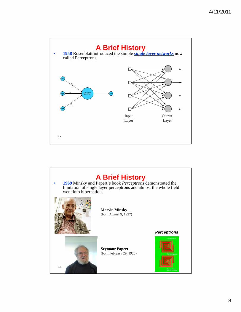
A Brief History• 1958 Rosenblatt introduced the simple single layer networks now
called Perceptrons.
Frank Rosenblatt(11 July 1928 – 1971)
14
2006 - LAWRENCE J. FOGEL2007 - JAMES C. BEZDEK2008 - TEUVO KOHONEN2009 - JOHN J. HOPFIELD2010 - MICHIO SUGENO
4/11/2011
8
A Brief History• 1958 Rosenblatt introduced the simple single layer networks now
called Perceptrons.
15
A Brief History• 1969 Minsky and Papert’s book Perceptrons demonstrated the
limitation of single layer perceptrons and almost the whole field went into hibernation.
Marvin Minsky (born August 9, 1927)
Perceptrons
16
Seymour Papert(born February 29, 1928)

4/11/2011
9
A Brief History• 1982 Hopfield published a series of papers on Hopfield networks.
John Joseph Hopfield(born July 15, 1933)
17 A Hopfield Net
He was awarded the Dirac Medal of the ICTP in 2001.
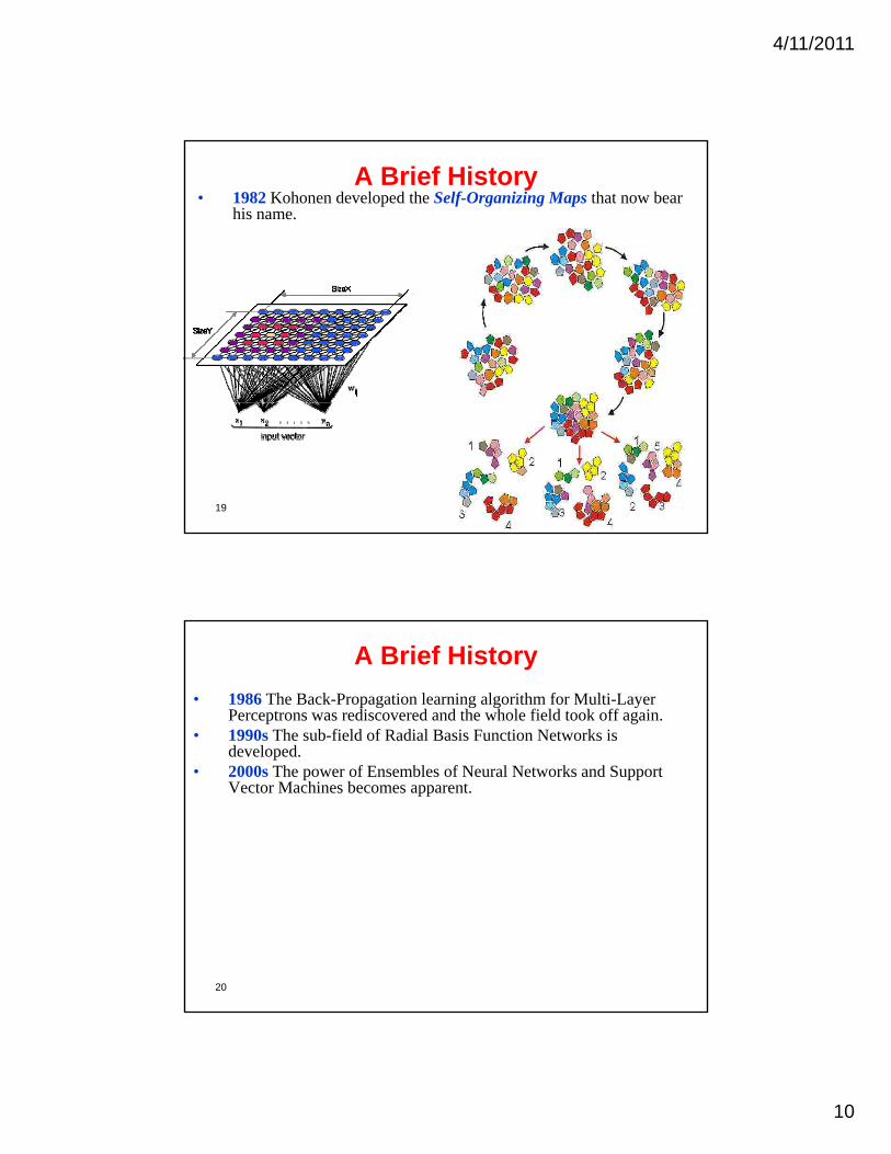
A Brief History• 1982 Kohonen developed the Self-Organizing Maps that now bear
his name.
Teuvo Kohonen(born July 11, 1934)
18 S.O.M
Self-Organizing Maps
New ed.: 2001
4/11/2011
10
A Brief History• 1982 Kohonen developed the Self-Organizing Maps that now bear
his name.
19
S.O.M
A Brief History
• 1986 The Back-Propagation learning algorithm for Multi-Layer Perceptrons was rediscovered and the whole field took off again.
• 1990s The sub-field of Radial Basis Function Networks is developeddeveloped.
• 2000s The power of Ensembles of Neural Networks and Support Vector Machines becomes apparent.
20
4/11/2011
1
Artificial Neural NetworksArtificial Neural Networks
Lecture 3
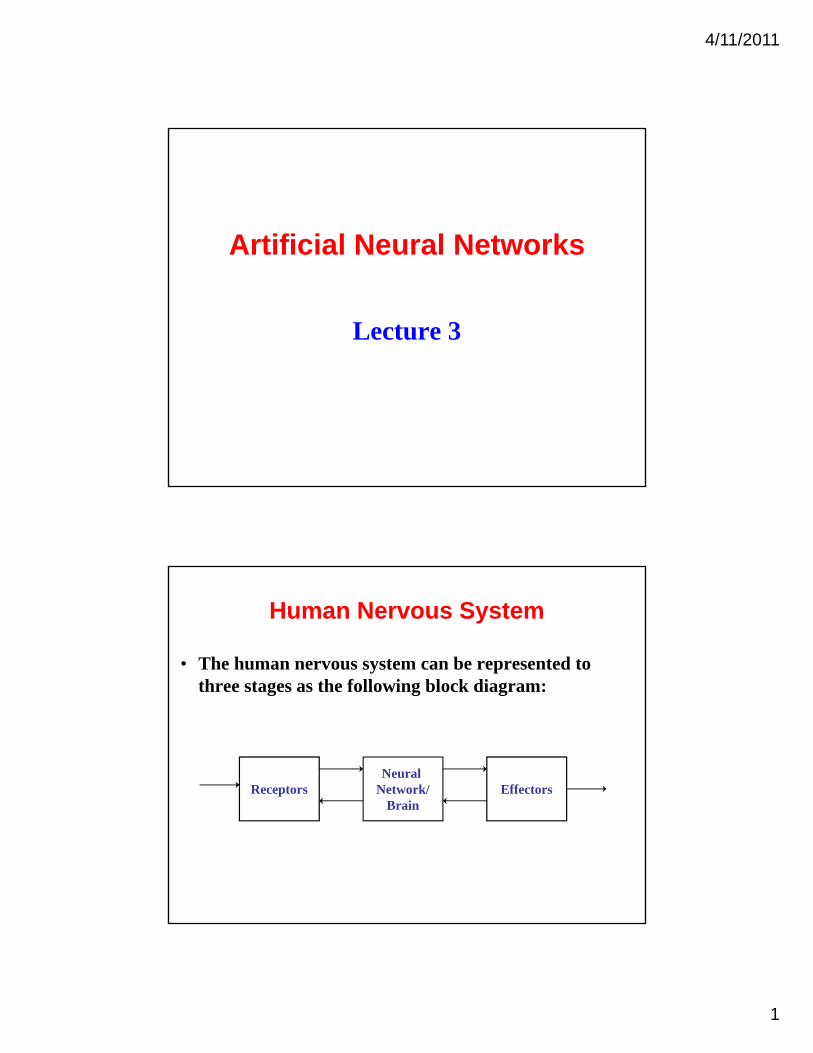
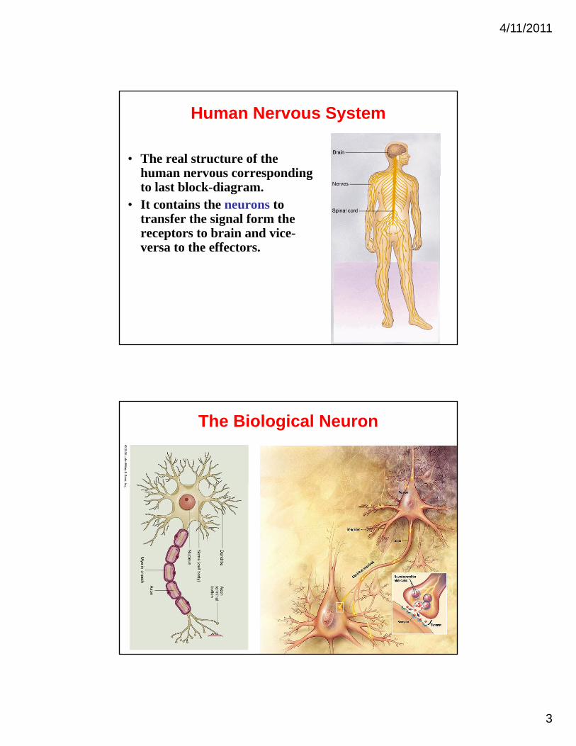
Human Nervous System
• The human nervous system can be represented to three stages as the following block diagram:three stages as the following block diagram:
ReceptorsNeural
Network/Brain
EffectorsBrain
4/11/2011
2
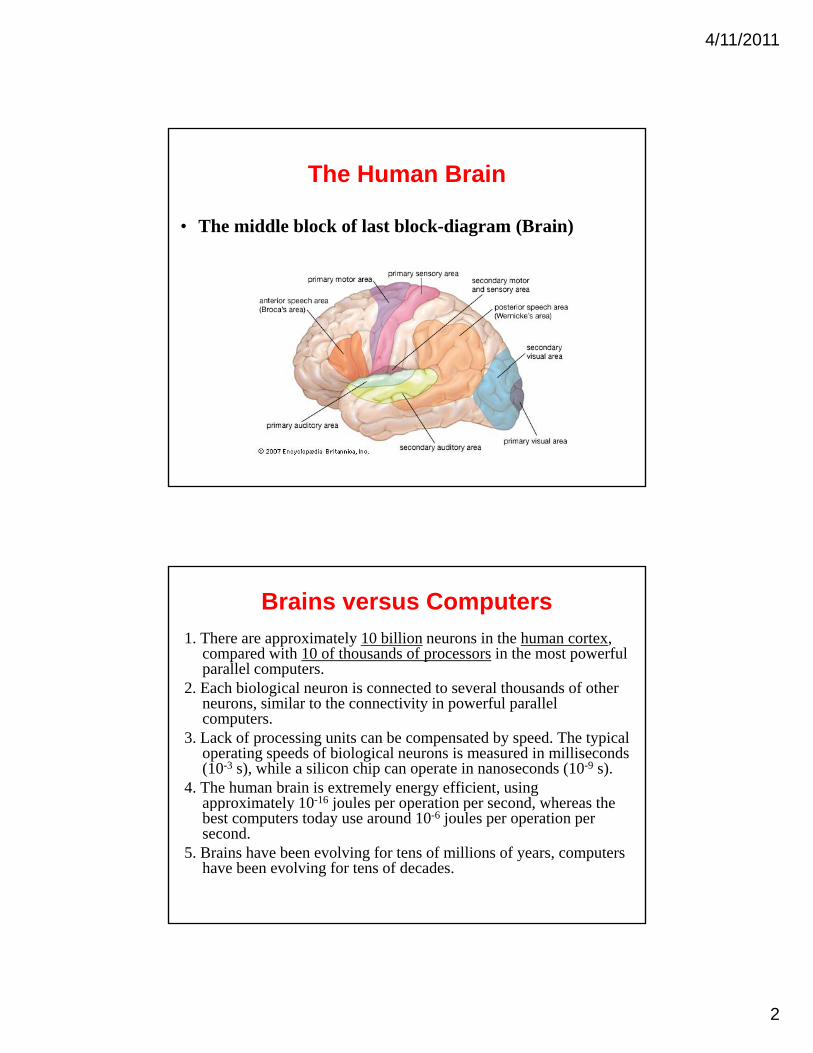
The Human Brain
• The middle block of last block-diagram (Brain)
Brains versus Computers
1. There are approximately 10 billion neurons in the human cortex, compared with 10 of thousands of processors in the most powerful parallel computers.
2 E h bi l i l i t d t l th d f th2. Each biological neuron is connected to several thousands of other neurons, similar to the connectivity in powerful parallel computers.
3. Lack of processing units can be compensated by speed. The typical operating speeds of biological neurons is measured in milliseconds (10-3 s), while a silicon chip can operate in nanoseconds (10-9 s).
4. The human brain is extremely energy efficient, using approximately 10-16 joules per operation per second whereas theapproximately 10 joules per operation per second, whereas the best computers today use around 10-6 joules per operation per second.
5. Brains have been evolving for tens of millions of years, computers have been evolving for tens of decades.
4/11/2011
3
Human Nervous System
• The real structure of the human nervous correspondinghuman nervous corresponding to last block-diagram.
• It contains the neurons to transfer the signal form the receptors to brain and vice-versa to the effectors.
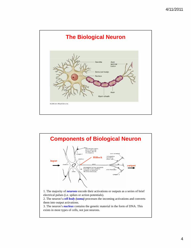
The Biological Neuron
4/11/2011
4
The Biological Neuron
Components of Biological Neuron
1. The majority of neurons encode their activations or outputs as a series of brief electrical pulses (i.e. spikes or action potentials).2. The neuron’s cell body (soma) processes the incoming activations and convertsthem into output activations.3. The neuron’s nucleus contains the genetic material in the form of DNA. Thisexists in most types of cells, not just neurons.
4/11/2011
5
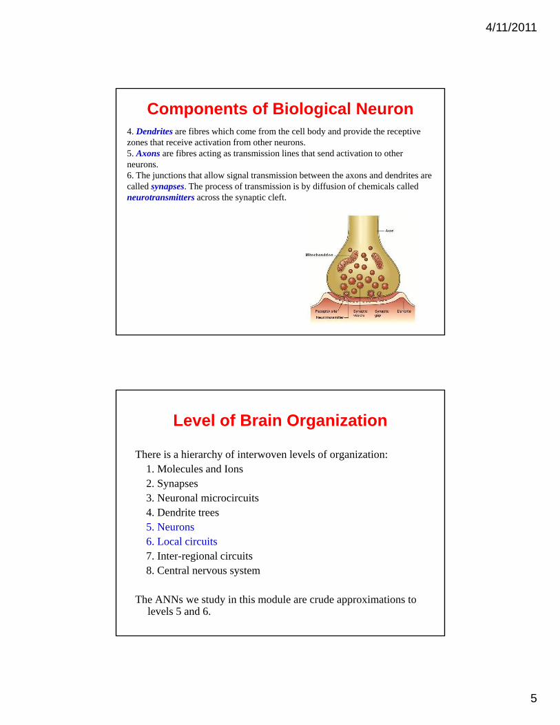
Components of Biological Neuron4. Dendrites are fibres which come from the cell body and provide the receptive zones that receive activation from other neurons.5. Axons are fibres acting as transmission lines that send activation to other neurons.6. The junctions that allow signal transmission between the axons and dendrites arecalled synapses. The process of transmission is by diffusion of chemicals calledneurotransmitters across the synaptic cleft.
Level of Brain Organization
There is a hierarchy of interwoven levels of organization:1. Molecules and Ions1. Molecules and Ions2. Synapses3. Neuronal microcircuits4. Dendrite trees5. Neurons6. Local circuits7 I t i l i it7. Inter-regional circuits8. Central nervous system
The ANNs we study in this module are crude approximations to levels 5 and 6.
4/11/2011
6
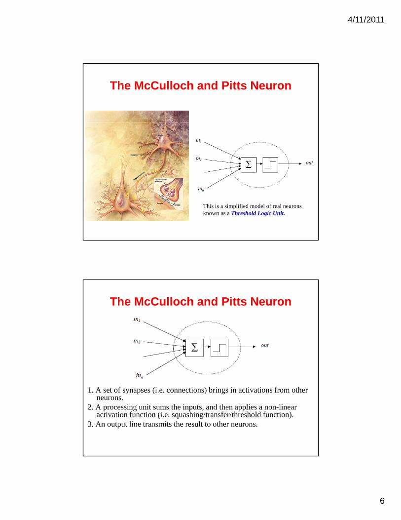
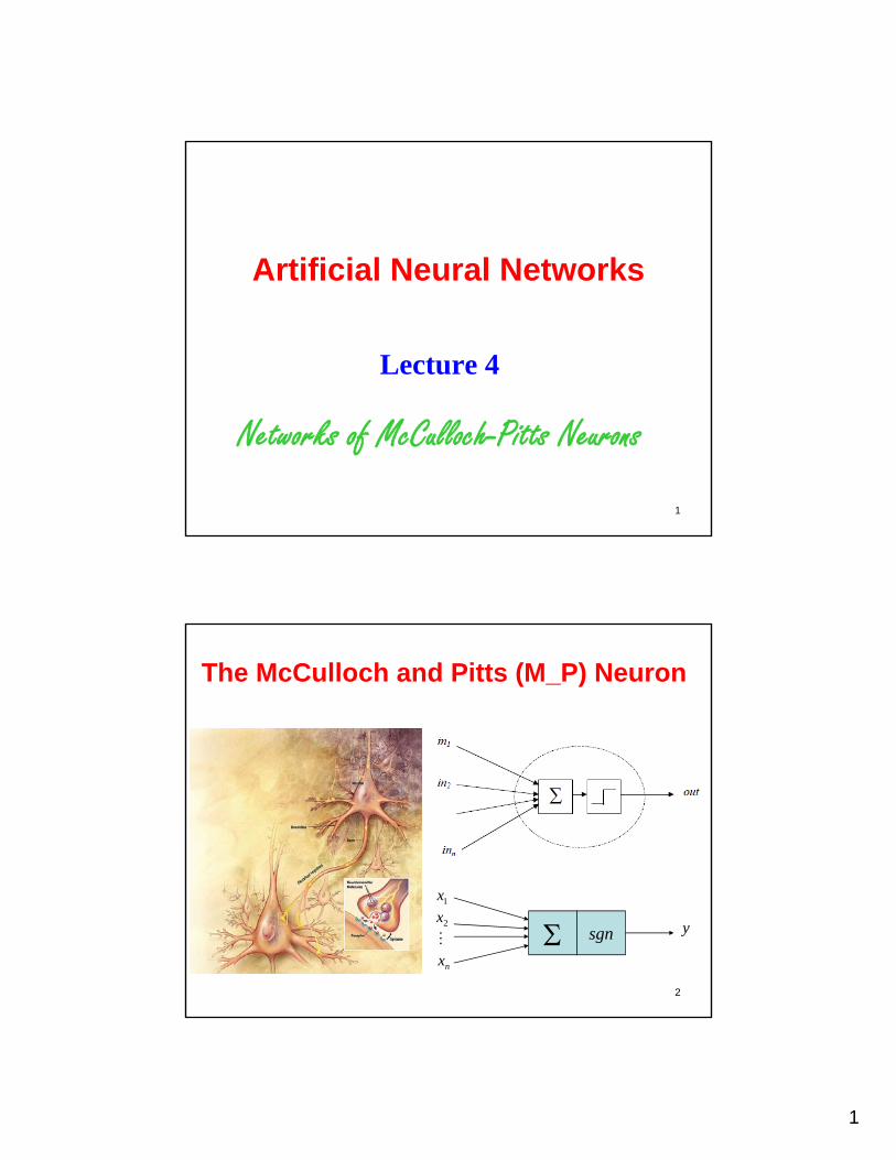
The McCulloch and Pitts Neuron
This is a simplified model of real neurons known as a Threshold Logic Unit.
The McCulloch and Pitts Neuron
1. A set of synapses (i.e. connections) brings in activations from other neuronsneurons.
2. A processing unit sums the inputs, and then applies a non-linear activation function (i.e. squashing/transfer/threshold function).
3. An output line transmits the result to other neurons.
4/11/2011
7
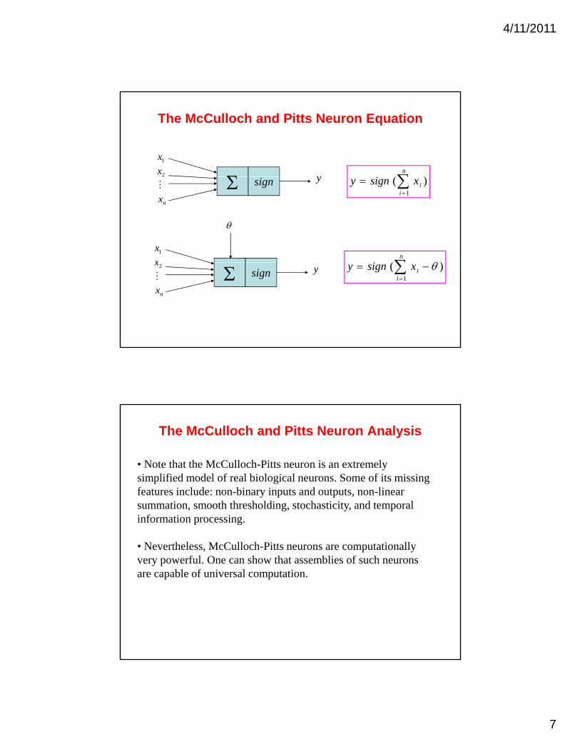
The McCulloch and Pitts Neuron Equation
1x
2x
y )(n
sign
nx y )(
1
i
ixsigny
1x
x
)( n
sign2x
nx y )(
1
i
ixsigny
The McCulloch and Pitts Neuron Analysis
• Note that the McCulloch-Pitts neuron is an extremely simplified model of real biological neurons. Some of its missing f t i l d bi i t d t t lifeatures include: non-binary inputs and outputs, non-linear summation, smooth thresholding, stochasticity, and temporal information processing.
• Nevertheless, McCulloch-Pitts neurons are computationally very powerful. One can show that assemblies of such neurons are capable of universal computationare capable of universal computation.
1
Artificial Neural NetworksArtificial Neural Networks
Lecture 4
1
Networks of McCulloch-Pitts Neurons
The McCulloch and Pitts (M_P) Neuron
2
sgn
1x
2x
nx y
2
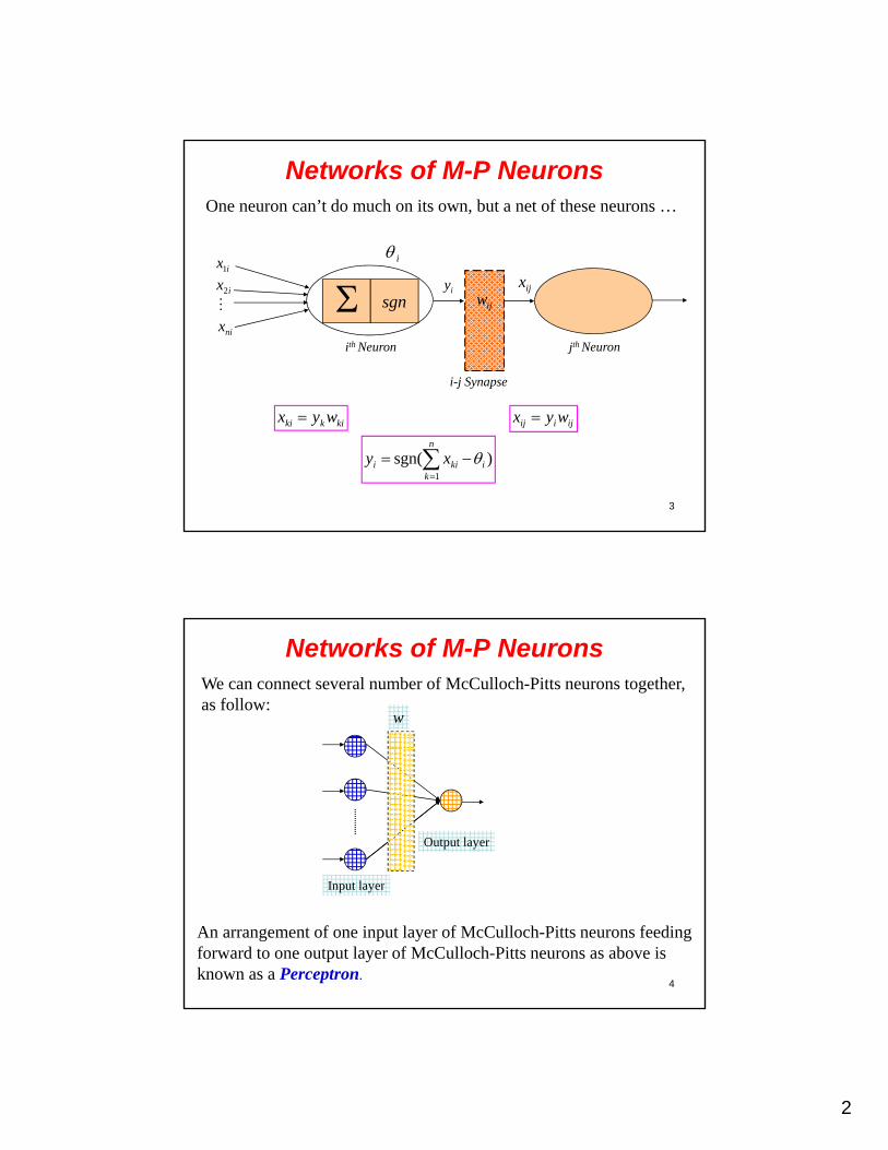
Networks of M-P NeuronsOne neuron can’t do much on its own, but a net of these neurons …
iix1
ijwijx
iy
sgn
i1
ix2
nix
ith Neuron jth Neuron
i-j Synapse
3
ijiij wyx
)sgn(1
n
kikii xy
kikki wyx
Networks of M-P NeuronsWe can connect several number of McCulloch-Pitts neurons together, as follow:
w
Output layer
4
An arrangement of one input layer of McCulloch-Pitts neurons feeding forward to one output layer of McCulloch-Pitts neurons as above is known as a Perceptron.
Input layer
3
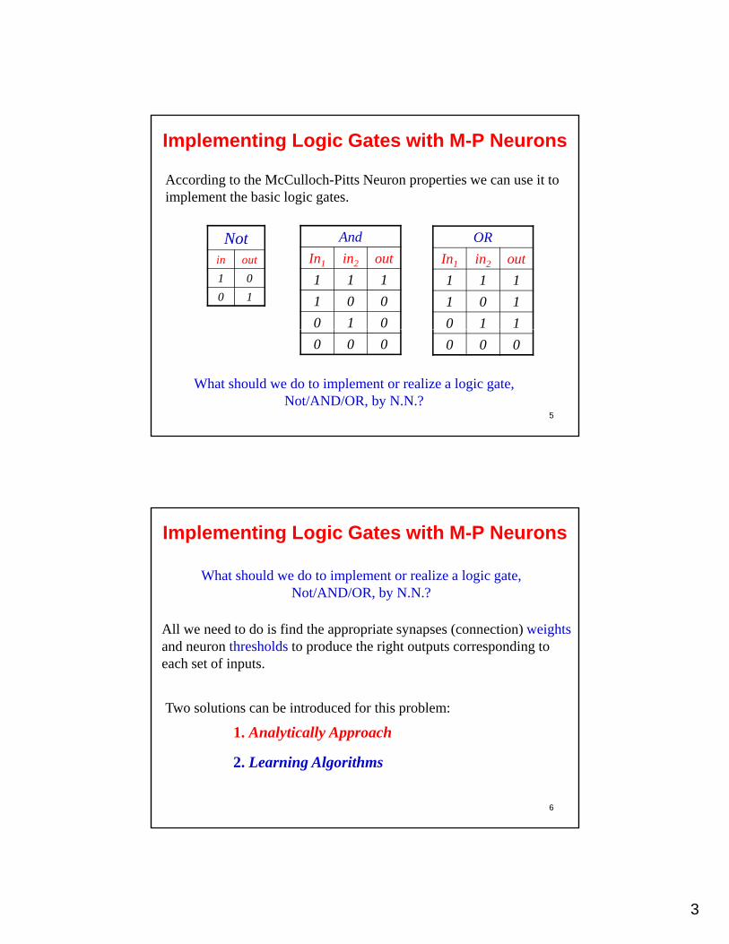
Implementing Logic Gates with M-P Neurons
According to the McCulloch-Pitts Neuron properties we can use it to implement the basic logic gates.
Notin out
1 0
0 1
And
In1 in2 out
1 1 1
1 0 0
0 1 0
OR
In1 in2 out
1 1 1
1 0 1
0 1 1
5
What should we do to implement or realize a logic gate, Not/AND/OR, by N.N.?
0 0 0 0 0 0
Implementing Logic Gates with M-P Neurons
What should we do to implement or realize a logic gate, Not/AND/OR, by N.N.?
All we need to do is find the appropriate synapses (connection) weightsand neuron thresholds to produce the right outputs corresponding to each set of inputs.
Two solutions can be introduced for this problem:
6
1. Analytically Approach
2. Learning Algorithms
4
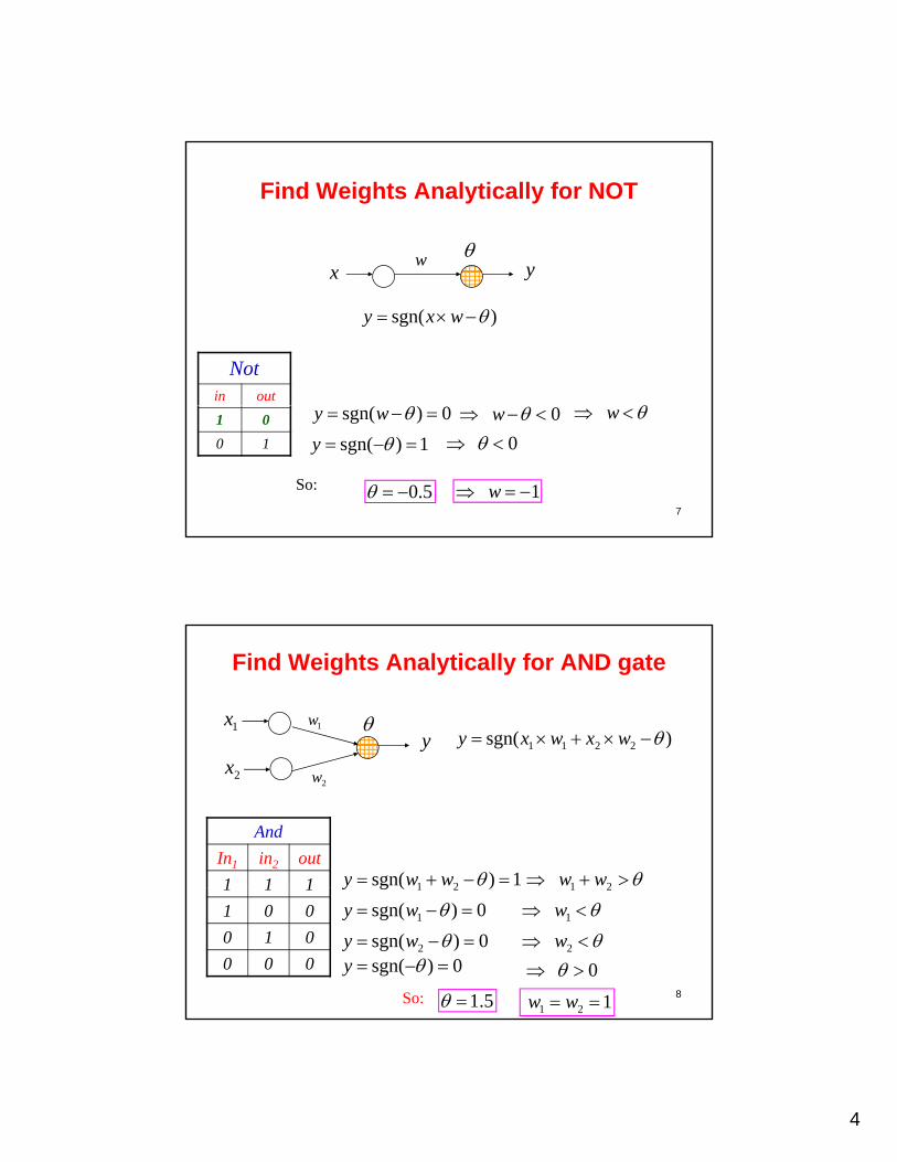
Find Weights Analytically for NOT
w yx yx
)sgn( wxy
Notin out
7
1 0
0 1 1)sgn( y
0)sgn( wy
0 0 w w
So: 5.0 1 w
Find Weights Analytically for AND gate
)sgn( 2211 wxwxy1w
y1x
21 ww
2x2w
And
In1 in2 out
1 1 1 1)sgn( 21 wwy
8
21
So: 5.1 1 21 ww
1 1 1
1 0 0
0 1 0
0 0 0
)g ( 21y
0)sgn( 1 wy
0)sgn( 2 wy0)sgn( y
1 w
2 w
0
5
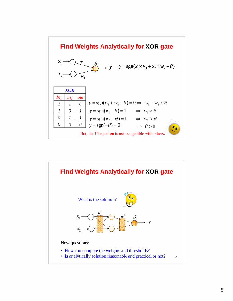
Find Weights Analytically for XOR gate
)sgn( 2211 wxwxy )sgn( 2211 wxwxy1w
y1x 1w
y1x
21 ww
XOR
In1 in2 out
1 1 0 0)sgn( 21 wwy
2x2w2x2w
9
21
But, the 1st equation is not compatible with others.
1 1 0
1 0 1
0 1 1
0 0 0
)g ( 21y
1)sgn( 1 wy
1)sgn( 2 wy0)sgn( y
1 w
2 w
0
Find Weights Analytically for XOR gate
What is the solution?
2w y
1x
2x
1w
10
2x
New questions:
• How can compute the weights and thresholds?• Is analytically solution reasonable and practical or not?
6
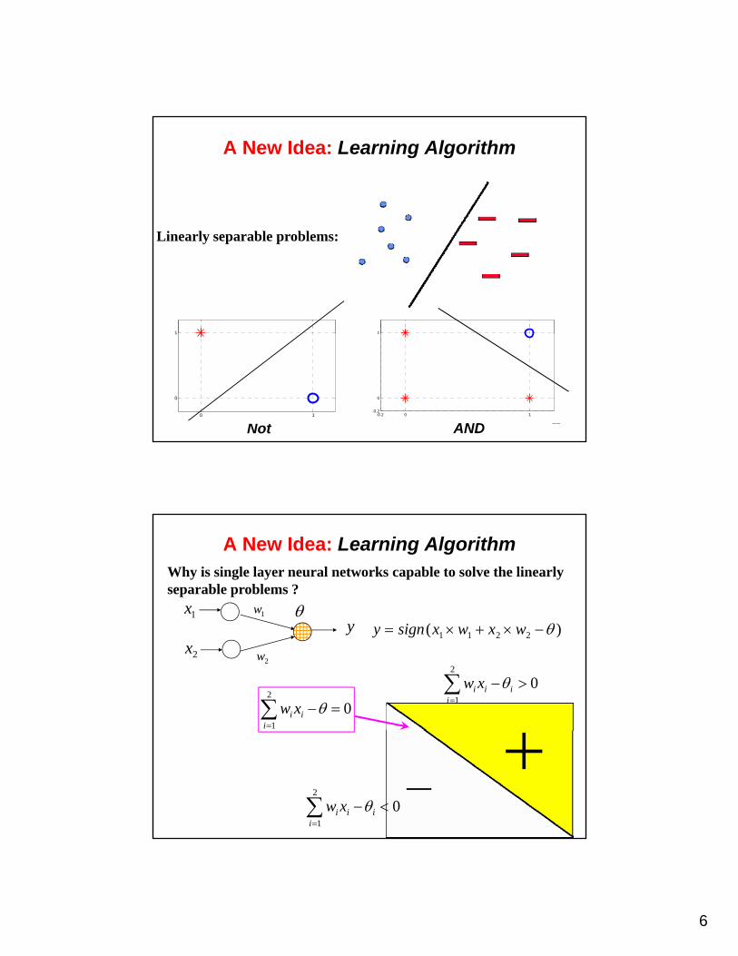
A New Idea: Learning Algorithm
Linearly separable problems:
1 1
11Not
0 1
0
1
-0.2 0 1-0.2
0
1
AND
A New Idea: Learning AlgorithmWhy is single layer neural networks capable to solve the linearly separable problems ?
1w 1x)( 2211 wxwxsignyy
2x2w
02
1
i
ii xw
02
1
ii
ii xw
120
2
1
ii
ii xw
7
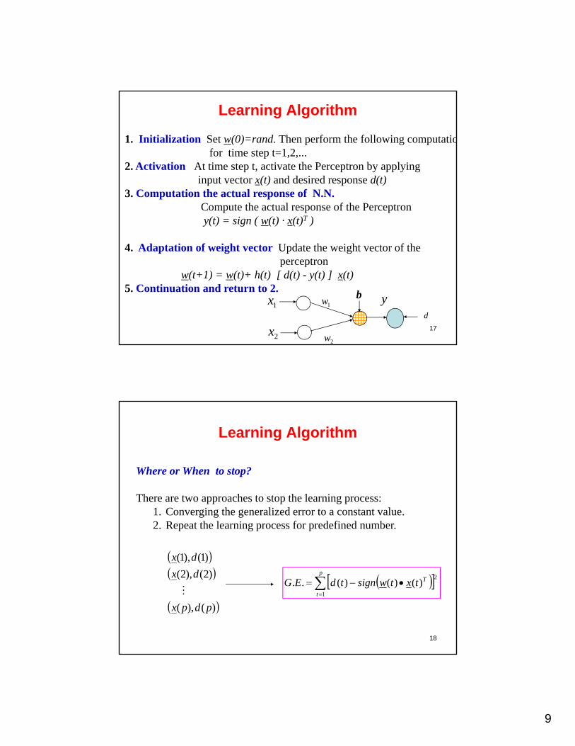
Learning Algorithm
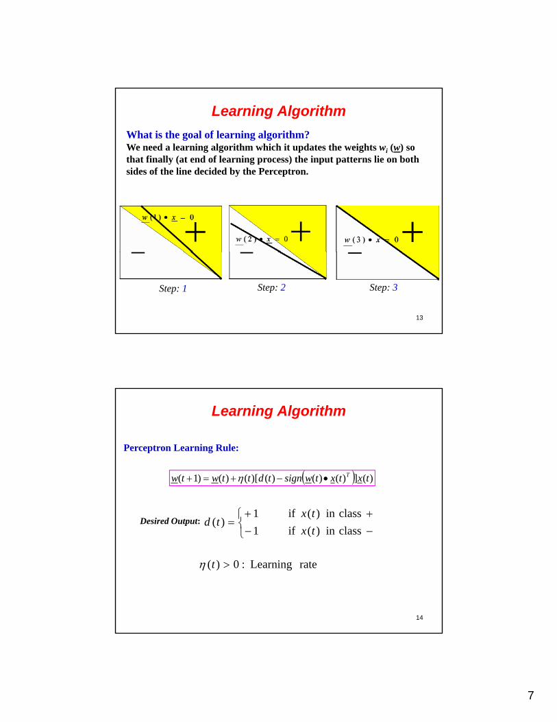
What is the goal of learning algorithm?We need a learning algorithm which it updates the weights wi (w) so that finally (at end of learning process) the input patterns lie on both id f th li d id d b th P tsides of the line decided by the Perceptron.
13
Step: 1 Step: 2 Step: 3
Learning Algorithm
Perceptron Learning Rule:
)(])()()()[()()1( txtxtwsigntdttwtw T
classin )( if1
classin )( if1)(
tx
txtdDesired Output:
14
rate Learning :0)( t
8
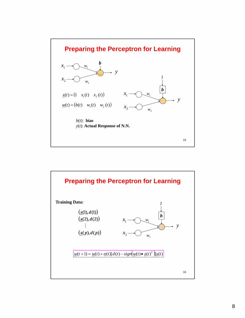
Preparing the Perceptron for Learning
1w
y1x b
2x2w
)()(1)( 21 txtxtx
)()()()( 21 twtwtbtw
1w
y1x
2x2w
b
1
15
2
b(t): biasy(t): Actual Response of N.N.
Preparing the Perceptron for Learning
1Training Data:
)(),(
)2(),2(
)1(),1(
pdpx
dx
dx
1w
y1x
2x2w
b
)(),(
)2(),2(
)1(),1(
pdpx
dx
dx
16
)(])()()()[()()1( txtxtwsigntdttwtw T
9
Learning Algorithm
1. Initialization Set w(0)=rand. Then perform the following computatiofor time step t=1,2,...
2. Activation At time step t, activate the Perceptron by applying input vector x(t) and desired response d(t)
3. Computation the actual response of N.N.Compute the actual response of the Perceptrony(t) = sign ( w(t) · x(t)T )
4. Adaptation of weight vector Update the weight vector of the perceptron
17
perceptronw(t+1) = w(t)+ h(t) [ d(t) - y(t) ] x(t)
5. Continuation and return to 2.1w y
1x
2x2w
b
d
Learning Algorithm
Where or When to stop?
)2()2(
)1(),1(
d
dx
There are two approaches to stop the learning process:1. Converging the generalized error to a constant value.2. Repeat the learning process for predefined number.
18
)(),(
)2(),2(
pdpx
dx
p
t
TtxtwsigntdEG1
2)()()(..

10
Training Types
Two types of network training:
Sequential mode (on-line, stochastic, or per-pattern)Weights updated after each pattern is presented(Perceptron is in this class)
Batch mode (off-line or per-epoch)Weights updated after all pattern in a period is presented
19
1st Mini Project
1. By using the perceptron learning rule generate a N.N. to represent a NOT gate.
2. By using the perceptron learning rule generate a N.N. to represent a AND gateAND gate.
3. By using the perceptron learning rule generate a N.N. to represent a OR gate.
4. Please show that the generalized error converge to constant value after a learning process.
5. Please test the above N.N.s by testing data?6. Please check the above N. N.s with data which added to noise.7 R t th l i f b N N i b th ith d ith t
20
7. Repeat the learning process for above N.N.s in both with and without bias.
8. Please plot the updated weights.
4/11/2011
1
Artificial Neural NetworksArtificial Neural Networks
Lecture 5
Activation Functions
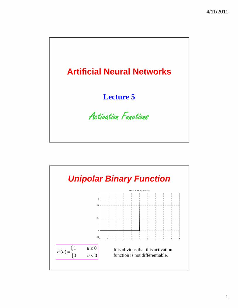
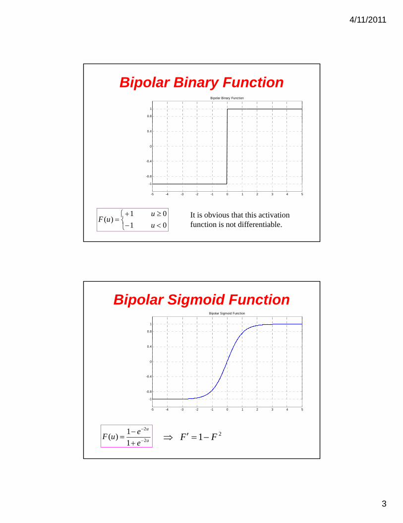
Unipolar Binary Function
1
Unipolar Binary Function
0
0.4
0.8
-5 -4 -3 -2 -1 0 1 2 3 4 5-0.2
00
01)(
u
uuF It is obvious that this activation
function is not differentiable.
4/11/2011
2
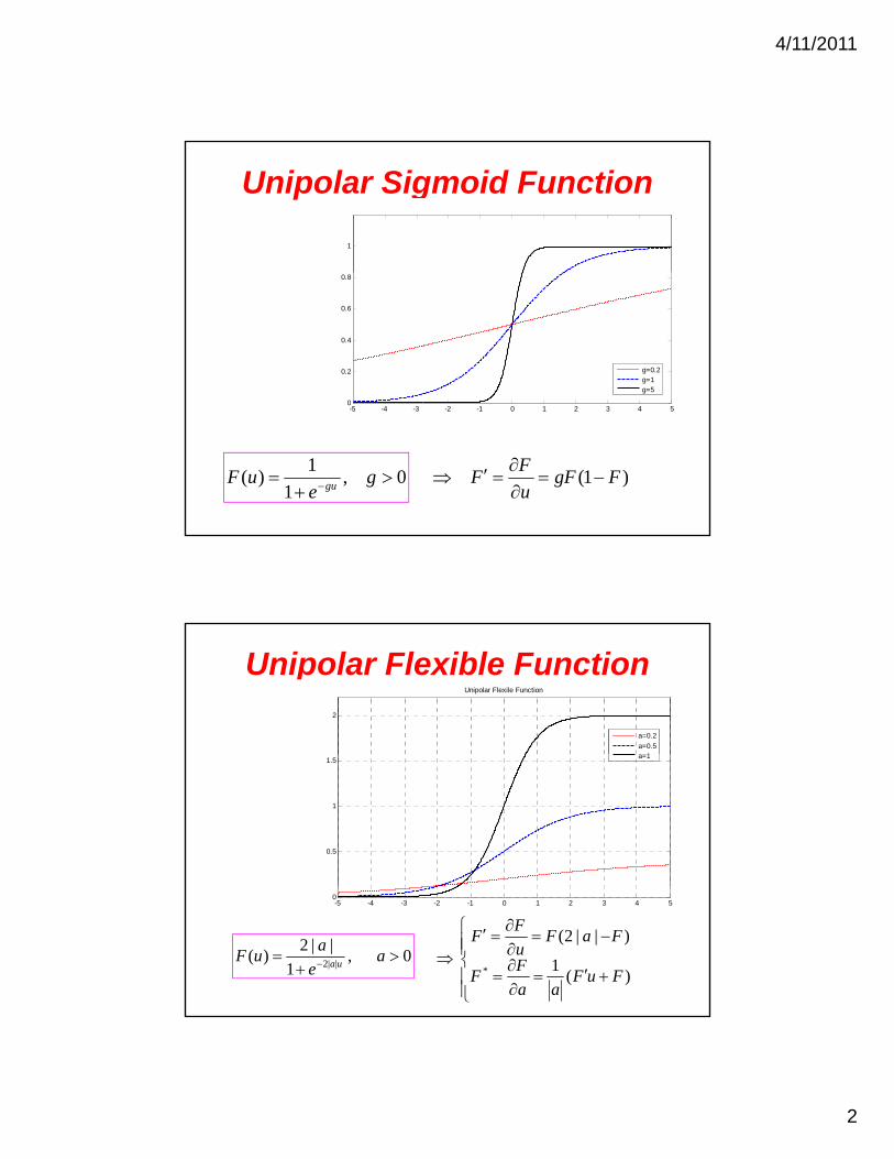
Unipolar Sigmoid Function
1
0
0.2
0.4
0.6
0.8
g=0.2g=1g=5
-5 -4 -3 -2 -1 0 1 2 3 4 50
)1( FgFu
FF
0 ,1
1)(
g
euF
gu
Unipolar Flexible Function2
Unipolar Flexile Function
a=0.2
a=0.51
0.5
1
1.5a=1
-5 -4 -3 -2 -1 0 1 2 3 4 50
0 ,1
||2)(
||2
a
e
auF
ua
)(1
)||2(
* FuFaa
FF
FaFu
FF
4/11/2011
3
Bipolar Binary Function
0.8
1
Bipolar Binary Function
-0.8
-0.4
0
0.4
01
01)(
u
uuF
-5 -4 -3 -2 -1 0 1 2 3 4 5
-1
It is obvious that this activation function is not differentiable.
Bipolar Sigmoid Function
0.8
1
Bipolar Sigmoid Function
-1
-0.8
-0.4
0
0.4
-5 -4 -3 -2 -1 0 1 2 3 4 5
1
u
u
e
euF
2
2
1
1)(
21 FF
4/11/2011
4
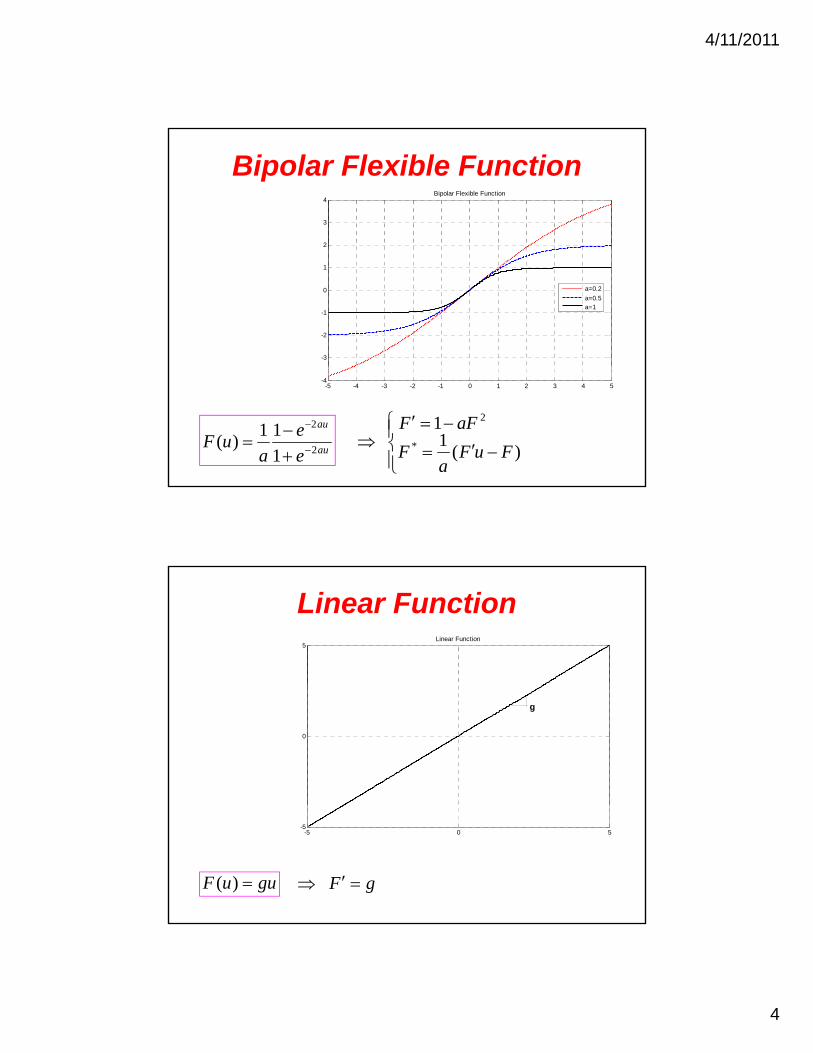
Bipolar Flexible Function
2
3
4Bipolar Flexible Function
-3
-2
-1
0
1
a=0.2
a=0.5a=1
-5 -4 -3 -2 -1 0 1 2 3 4 5-4
au
au
e
e
auF
2
2
1
11)(
)(1
1 *
2
FuFa
F
aFF
Linear Function5
Linear Function
0
g
guuF )( gF
-5 0 5-5
4/11/2011
5
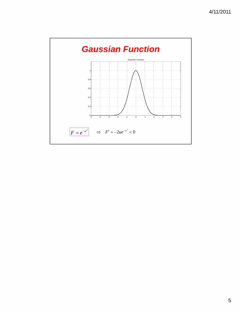
Gaussian Function
1
Gaussian Function
0.2
0.4
0.6
0.8
-5 -4 -3 -2 -1 0 1 2 3 4 50
2ueF 02 2
uueF
1
Artificial Neural NetworksArtificial Neural Networks
Lecture 6
1
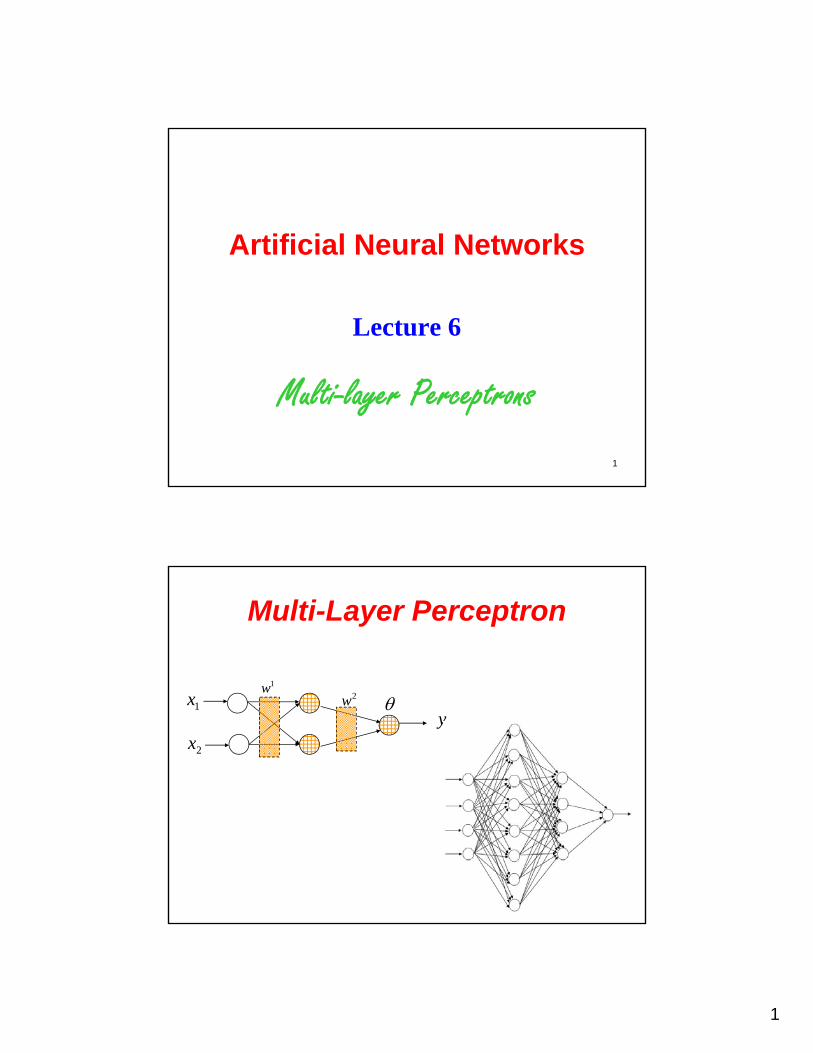
Multi-layer Perceptrons
Multi-Layer Perceptron
1
2w y
1x
2x
1w
2
2
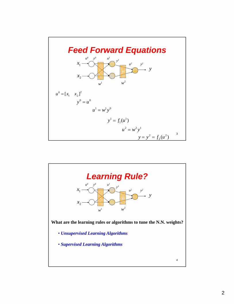
Feed Forward Equations
y1x
u1
u2
u0 y0
y1
y2
2w1w
2x
Txxu ][ 210
00 uy
3
011 ywu
)( 11
1 ufy 122 ywu
)( 22
2 ufyy
Learning Rule?
y1x
u1
u2
u0 y0
y1
y2
2w1w
2x
What are the learning rules or algorithms to tune the N.N. weights?
U i d L i Al ith
4
• Unsupervised Learning Algorithms
• Supervised Learning Algorithms
3
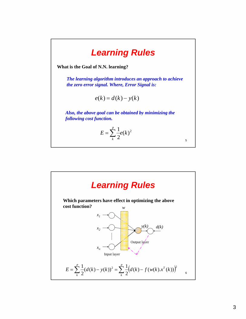
Learning Rules
What is the Goal of N.N. learning?
The learning algorithm introduces an approach to achieve the zero error signal. Where, Error Signal is:
)()()( kykdke
Al h b l b b i d b i i i i h
5
Also, the above goal can be obtained by minimizing the following cost function.
2)(2
1keE
p
k
Learning Rules
Which parameters have effect in optimizing the above cost function? wcost function? w
Output layer
y(k) d(k)
x1
x2
6 22 ))().(()(
2
1))()((
2
1kxkwfkdkykdE T
p
k
p
k
Input layer
p y
xn
4
Learning Rules
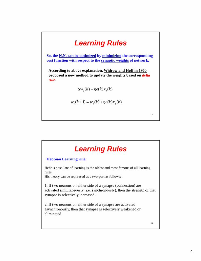
So, the N.N. can be optimized by minimizing the corresponding cost function with respect to the synaptic weights of network.cost function with respect to the synaptic weights of network.
)()()( kxkekw jj
According to above explanation, Widrow and Hoff in 1960proposed a new method to update the weights based on delta rule.
7
)()()( jj
)()()()1( kxkekwkw jjj
Learning RulesHebbian Learning rule:
Hebb’s postulate of learning is the oldest and most famous of all learning rules.His theory can be rephrased as a two-part as follows:
1. If two neurons on either side of a synapse (connection) are activated simultaneously (i.e. synchronously), then the strength of that synapse is selectively increased.
8
2. If two neurons on either side of a synapse are activated asynchronously, then that synapse is selectively weakened or eliminated.
5
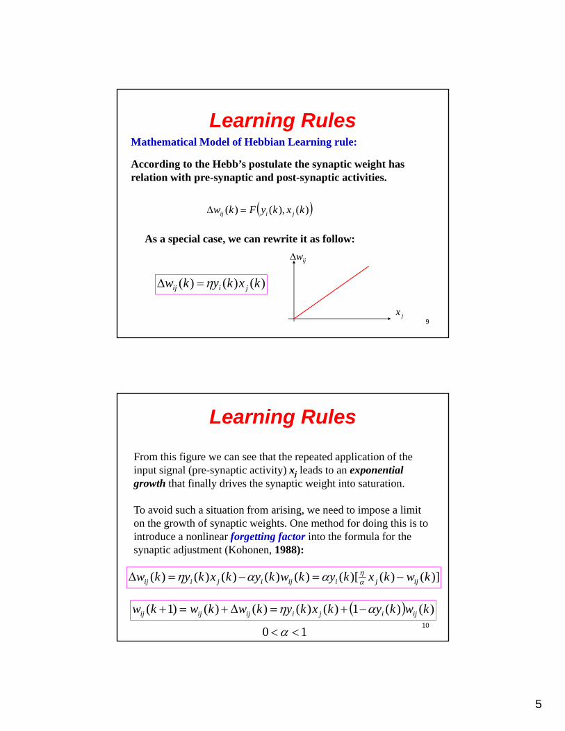
Learning RulesMathematical Model of Hebbian Learning rule:
According to the Hebb’s postulate the synaptic weight has
)(),()( kxkyFkw jiij
relation with pre-synaptic and post-synaptic activities.
As a special case, we can rewrite it as follow:
9
)()()( kxkykw jiij
ijw
jx
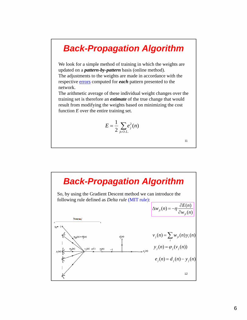
Learning Rules
From this figure we can see that the repeated application of the input signal (pre-synaptic activity) xj leads to an exponential p g (p y p y) j pgrowth that finally drives the synaptic weight into saturation.
To avoid such a situation from arising, we need to impose a limit on the growth of synaptic weights. One method for doing this is to introduce a nonlinear forgetting factor into the formula for the synaptic adjustment (Kohonen, 1988):
10
)]()()[()()()()()( kwkxkykwkykxkykw ijjiijijiij
)()(1)()()()()1( kwkykxkykwkwkw ijijiijijij
10
6
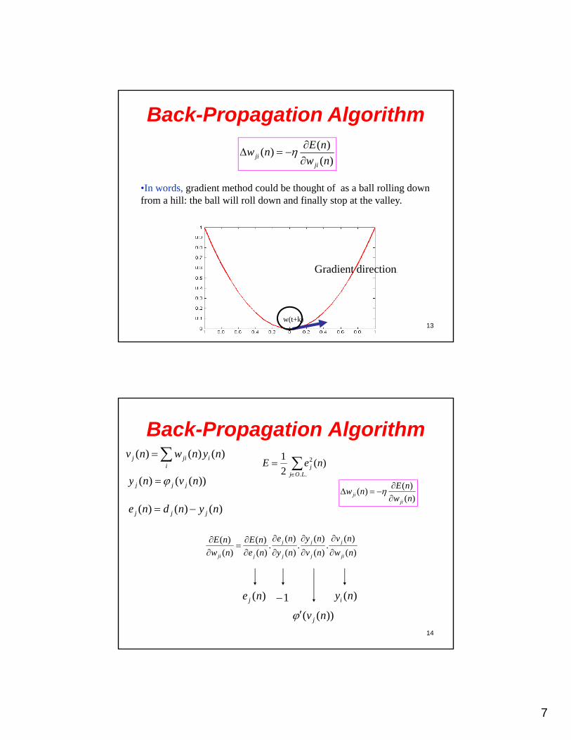
Back-Propagation Algorithm
We look for a simple method of training in which the weights are updated on a pattern-by-pattern basis (online method). The adjustments to the weights are made in accordance with theThe adjustments to the weights are made in accordance with the respective errors computed for each pattern presented to the network.The arithmetic average of these individual weight changes over the training set is therefore an estimate of the true change that would result from modifying the weights based on minimizing the cost function E over the entire training set
11
..
2 )(2
1
LOjj neE
function E over the entire training set.
Back-Propagation Algorithm
)()(
nEnw
So, by using the Gradient Descent method we can introduce the following rule defined as Delta rule (MIT rule):
)()(
nwnw
jiji
i
ijij nynwnv )()()(
12
))(()( nvny jjj
)()()( nyndne jjj
7
)(
)()(
nw
nEnw
jiji
Back-Propagation Algorithm
•In words, gradient method could be thought of as a ball rolling down from a hill: the ball will roll down and finally stop at the valley.
13
Gradient direction
w(t)
Gradient direction
w(t+1)
Gradient direction
w(t+k)
Back-Propagation Algorithm
iijij nynwnv )()()(
))(()( nvny
..
2 )(2
1
LOjj neE
)(
)(.
)(
)(.
)(
)(.
)(
)(
)(
)(
nw
nv
nv
ny
ny
ne
ne
nE
nw
nE
ji
j
j
j
j
j
jji
)(
)()(
nw
nEnw
jiji
))(()( nvny jjj
)()()( nyndne jjj
14
)(ne j 1
))(( nv j
)(nyi
8
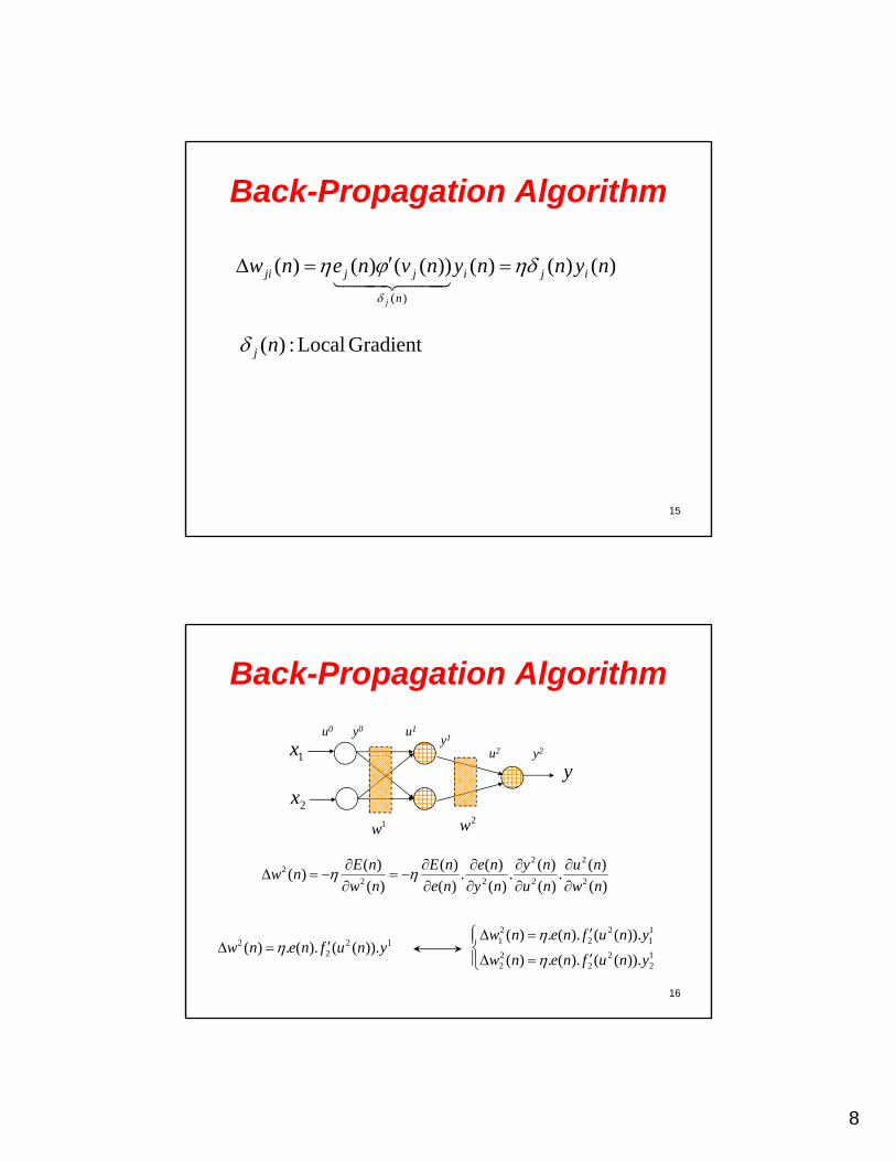
Back-Propagation Algorithm
)()()())(()()( nynnynvnenw ijijjji )()()())(()()(
)(
yy iji
n
jjji
j
Gradient Local :)(nj
15
Back-Propagation Algorithm
1xu1
u2
u0 y0
y1
y2
2w1w
y1x
2x
u y
)(
)(.
)(
)(.
)(
)(.
)(
)(
)(
)()(
2
2
2
2
222
nw
nu
nu
ny
ny
ne
ne
nE
nw
nEnw
16
)()()()()( nwnunynenw
122
2 )).(().(.)( ynufnenw
12
22
22
11
22
21
)).(().(.)(
)).(().(.)(
ynufnenw
ynufnenw
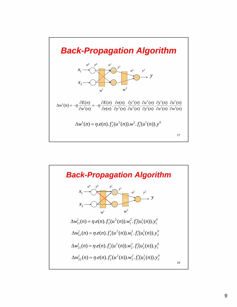
9
Back-Propagation Algorithm
1xu1
u2
u0 y0
y1
y2
2w1w
y1
2x
y
)(
)(.
)(
)(.
)(
)(.
)(
)(.
)(
)(.
)(
)(
)(
)()(
1
1
1
1
1
2
2
2
211 nunynunynenEnE
nw
17
)()()()()()()()(
111221 nwnunynunynenw
011
222
1 )).((.)).(().(.)( ynufwnufnenw
Back-Propagation Algorithm
y1x
u1
u2
u0 y0
y1
y2
2w1w
y
2x
01
111
21
22
111 )).((.)).(().(.)( ynufwnufnenw
02
111
21
22
112 )).((.)).(().(.)( ynufwnufnenw
18
2111212 ))(())(()()( yff
01
121
22
22
121 )).((.)).(().(.)( ynufwnufnenw
02
121
22
22
122 )).((.)).(().(.)( ynufwnufnenw
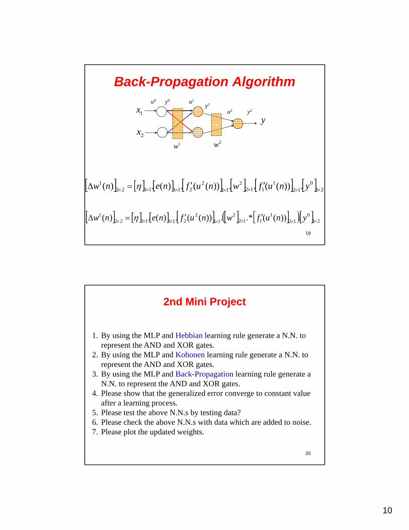
10
Back-Propagation Algorithm
y1x
u1
u2
u0 y0
y1
y2
2w1w
y
2x
01221 ))(())(()()( ynufwnufnenw
19
2112112112111122 .))((..))((.)(.)( ynufwnufnenw
210
121
1122
112
21111221 .))((*..))((.)(.)( ynufwnufnenw
2nd Mini Project
1. By using the MLP and Hebbian learning rule generate a N.N. to represent the AND and XOR gatesrepresent the AND and XOR gates.
2. By using the MLP and Kohonen learning rule generate a N.N. to represent the AND and XOR gates.
3. By using the MLP and Back-Propagation learning rule generate a N.N. to represent the AND and XOR gates.
4. Please show that the generalized error converge to constant value after a learning process.
20
after a learning process.5. Please test the above N.N.s by testing data?6. Please check the above N.N.s with data which are added to noise.7. Please plot the updated weights.
1
Artificial Neural NetworksArtificial Neural Networks
Lecture 7
1
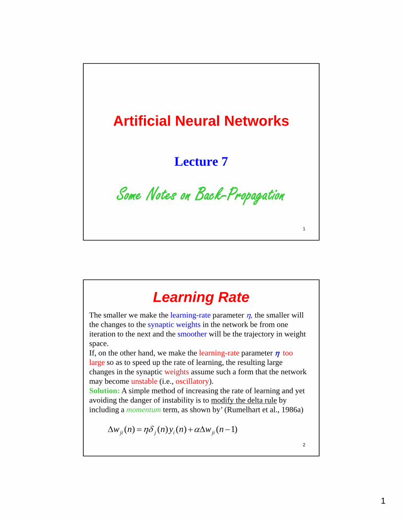
Some Notes on Back-Propagation
Learning RateThe smaller we make the learning-rate parameter the smaller will the changes to the synaptic weights in the network be from one iteration to the next and the smoother will be the trajectory in weight space.If, on the other hand, we make the learning-rate parameter too large so as to speed up the rate of learning, the resulting large changes in the synaptic weights assume such a form that the network may become unstable (i.e., oscillatory). Solution: A simple method of increasing the rate of learning and yet
idi h d f i bili i dif h d l l b
2
avoiding the danger of instability is to modify the delta rule by including a momentum term, as shown by’ (Rumelhart et al., 1986a)
)1()()()( nwnynnw jiijji
2
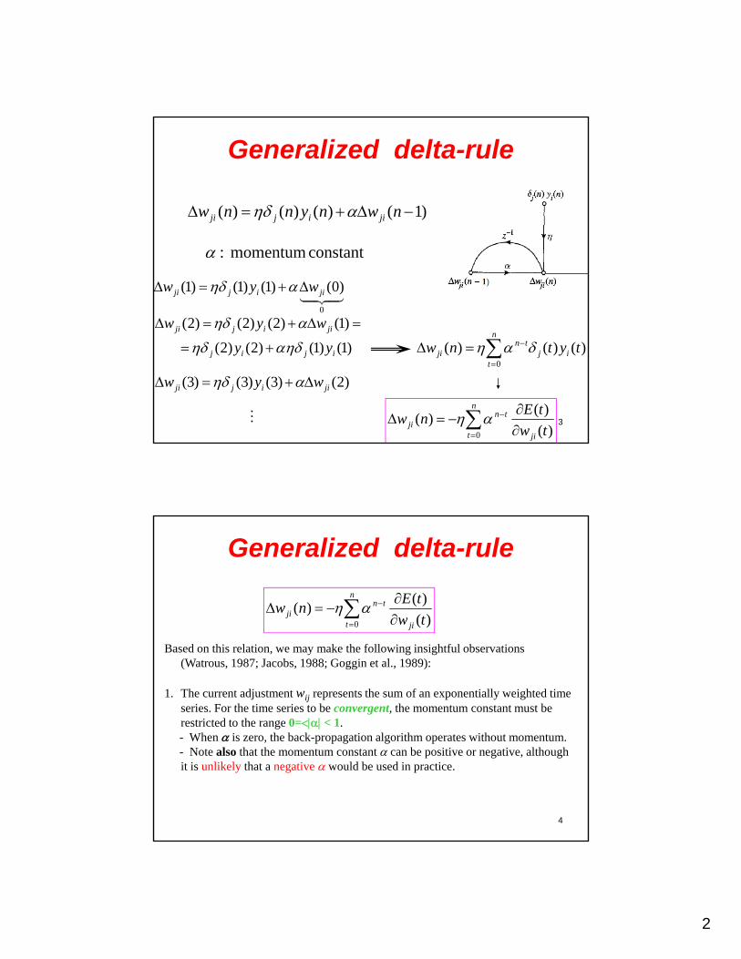
Generalized delta-rule
)1()()()( nwnynnw jiijji
constantmomentum :
n
0
)0()1()1()1( jiijji wyw
)1()2()2()2( jiijji wyw
3
n
tij
tnji tytnw
0
)()()( )1()1()2()2( ijij yy
)2()3()3()3( jiijji wyw
n
t ji
tnji tw
tEnw
0 )(
)()(
Generalized delta-rule
n
t ji
tnji tw
tEnw
0 )(
)()(
t ji tw0 )(
Based on this relation, we may make the following insightful observations (Watrous, 1987; Jacobs, 1988; Goggin et al., 1989):
1. The current adjustment wij represents the sum of an exponentially weighted time series. For the time series to be convergent, the momentum constant must be restricted to the range 0= < 1.
h i h b k i l i h i h
4
- When is zero, the back-propagation algorithm operates without momentum. - Note also that the momentum constant can be positive or negative, although it is unlikely that a negative would be used in practice.
3
Generalized delta-rule
n
t ji
tnji tw
tEnw
0 )(
)()( )1()()()( nwnynnw jiijji
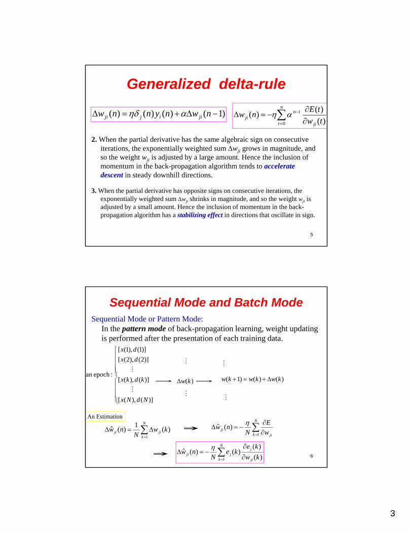
ji )(
2. When the partial derivative has the same algebraic sign on consecutive iterations, the exponentially weighted sum wji grows in magnitude, and so the weight wji is adjusted by a large amount. Hence the inclusion of momentum in the back-propagation algorithm tends to accelerate descent in steady downhill directions.
5
3. When the partial derivative has opposite signs on consecutive iterations, the exponentially weighted sum wji shrinks in magnitude, and so the weight wji is adjusted by a small amount. Hence the inclusion of momentum in the back-propagation algorithm has a stabilizing effect in directions that oscillate in sign.
Sequential Mode and Batch Mode
Sequential Mode or Pattern Mode:In the pattern mode of back-propagation learning, weight updating is performed after the presentation of each training data.
)](),([
)](),([
)]2(),2([
)]1(),1([
:epochan
NdNx
kdkx
dx
dx
)()()1( kwkwkw
)(kw
6
N
kjiji kw
Nnw
1
)(1
)(ˆ
N
k jiji w
E
Nnw
1
)(ˆ
N
k ji
jjji kw
keke
Nnw
1 )(
)()()(ˆ
An Estimation
4
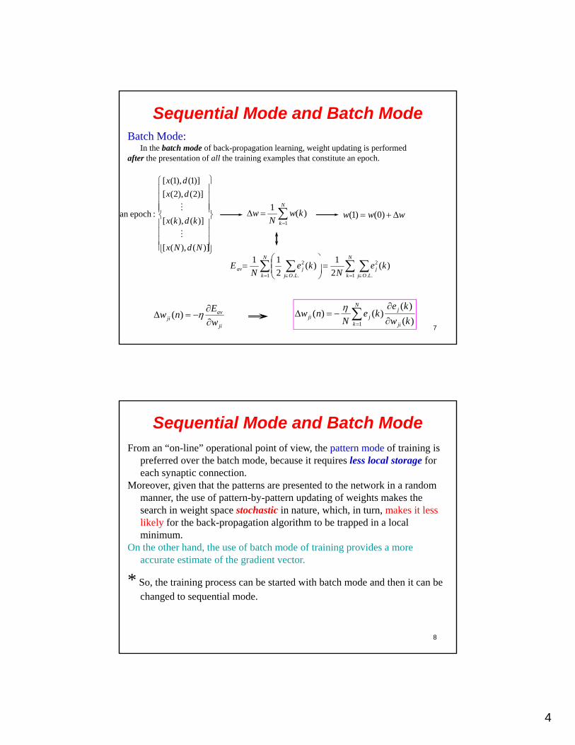
Sequential Mode and Batch Mode
Batch Mode:In the batch mode of back-propagation learning, weight updating is performed
after the presentation of all the training examples that constitute an epoch.
)](),([
)](),([
)]2(),2([
)]1(),1([
:epochan
NdNx
kdkx
dx
dx
N
k
kwN
w1
)(1
www )0()1(
NN 111
7ji
avji w
Enw
)(
N
k ji
jjji kw
keke
Nnw
1 )(
)()()(
k LOjj
k LOjjav ke
Nke
NE
1 ..
2
1 ..
2 )(2
1)(
2
11
Sequential Mode and Batch ModeFrom an “on-line” operational point of view, the pattern mode of training is
preferred over the batch mode, because it requires less local storage for each synaptic connection.
Moreover given that the patterns are presented to the network in a randomMoreover, given that the patterns are presented to the network in a random manner, the use of pattern-by-pattern updating of weights makes the search in weight space stochastic in nature, which, in turn, makes it less likely for the back-propagation algorithm to be trapped in a local minimum.
On the other hand, the use of batch mode of training provides a more accurate estimate of the gradient vector.
8
* So, the training process can be started with batch mode and then it can be changed to sequential mode.

5
Stopping Criteria
• The back-propagation algorithm is considered to have converged when the Euclidean norm of the gradient vector reaches a sufficiently small gradient threshold
• The back-propagation algorithm is considered to have converged when the absolute rate of change in the average squared error (Eav) per epoch i ffi i tl ll
gradient threshold.
The drawback of this convergence criterion is that, for successful trials, learning times may be long.
9
is sufficiently small.
Typically, the rate of change in the average squared error is considered to be small enough if it lies in the range of 0.1 to 1 percent per epoch; sometimes, a value as small as 0.01 percent per epoch is used.
Stopping Criteria
• Another useful criterion for convergence is as follows. After each learning iteration, the network is tested for its generalization performance The learning process is stopped when the generalizationperformance. The learning process is stopped when the generalization performance is adequate.
10
6
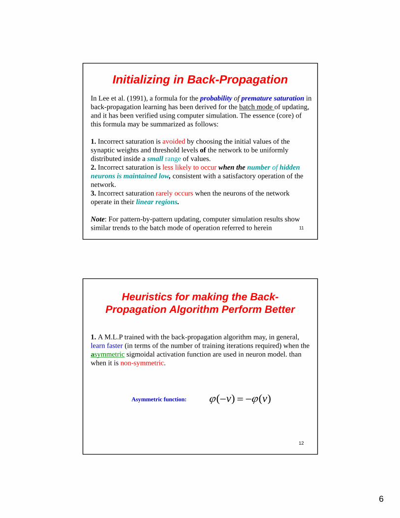
Initializing in Back-Propagation
In Lee et al. (1991), a formula for the probability of premature saturation in back-propagation learning has been derived for the batch mode of updating, and it has been verified using computer simulation. The essence (core) of hi f l b i d f llthis formula may be summarized as follows:
1. Incorrect saturation is avoided by choosing the initial values of the synaptic weights and threshold levels of the network to be uniformly distributed inside a small range of values.2. Incorrect saturation is less likely to occur when the number of hidden neurons is maintained low, consistent with a satisfactory operation of the
11
network.3. Incorrect saturation rarely occurs when the neurons of the network operate in their linear regions.
Note: For pattern-by-pattern updating, computer simulation results show similar trends to the batch mode of operation referred to herein
Heuristics for making the Back-Propagation Algorithm Perform Better
1 A M L P trained with the back propagation algorithm may in general1. A M.L.P trained with the back-propagation algorithm may, in general,learn faster (in terms of the number of training iterations required) when the asymmetric sigmoidal activation function are used in neuron model. than when it is non-symmetric.
)()(
12
)()( vv Asymmetric function:
7
Heuristics for making the Back-Propagation Algorithm Perform Better
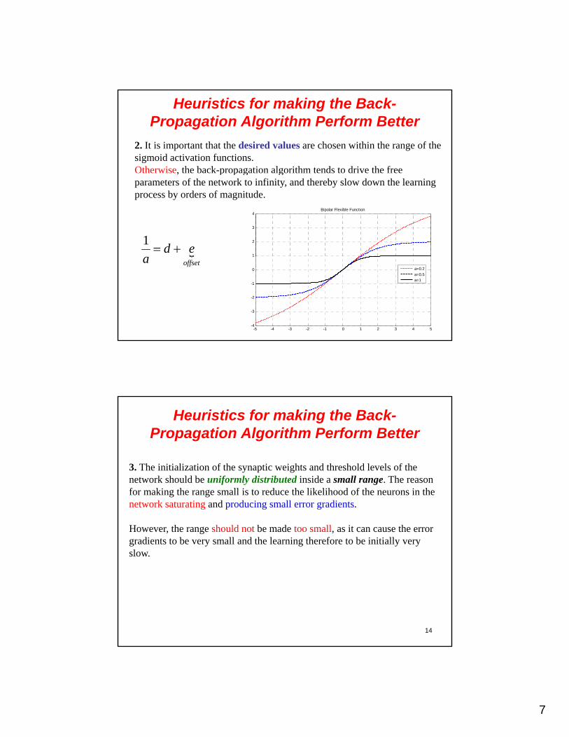
2. It is important that the desired values are chosen within the range of the sigmoid activation functions.Otherwise, the back-propagation algorithm tends to drive the free , p p g gparameters of the network to infinity, and thereby slow down the learningprocess by orders of magnitude.
eda
1
1
2
3
4Bipolar Flexible Function
13
offseta
-5 -4 -3 -2 -1 0 1 2 3 4 5-4
-3
-2
-1
0
a=0.2
a=0.5a=1
Heuristics for making the Back-Propagation Algorithm Perform Better
3. The initialization of the synaptic weights and threshold levels of the network should be uniformly distributed inside a small range The reasonnetwork should be uniformly distributed inside a small range. The reason for making the range small is to reduce the likelihood of the neurons in the network saturating and producing small error gradients.
However, the range should not be made too small, as it can cause the error gradients to be very small and the learning therefore to be initially very slow.
14
8
Heuristics for making the Back-Propagation Algorithm Perform Better
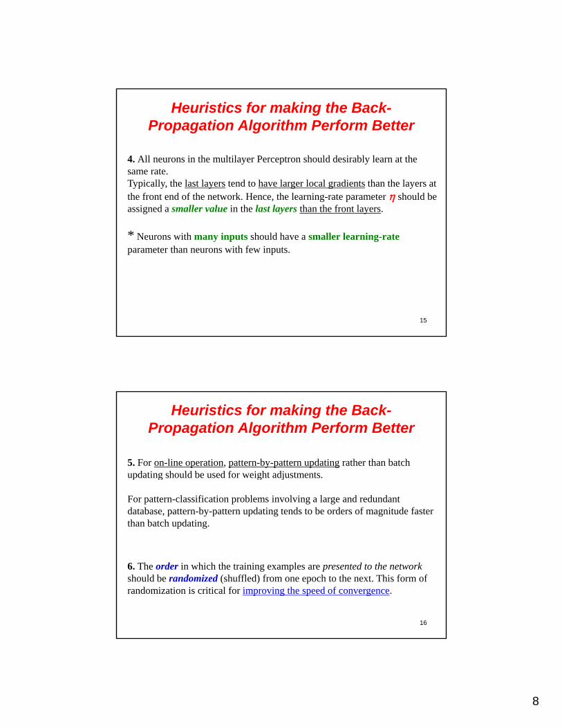
4. All neurons in the multilayer Perceptron should desirably learn at the same ratesame rate. Typically, the last layers tend to have larger local gradients than the layers at the front end of the network. Hence, the learning-rate parameter should be assigned a smaller value in the last layers than the front layers.
* Neurons with many inputs should have a smaller learning-rateparameter than neurons with few inputs.
15
p p
Heuristics for making the Back-Propagation Algorithm Perform Better
5. For on-line operation, pattern-by-pattern updating rather than batch updating should be used for weight adjustmentsupdating should be used for weight adjustments.
For pattern-classification problems involving a large and redundant database, pattern-by-pattern updating tends to be orders of magnitude fasterthan batch updating.
16
6. The order in which the training examples are presented to the networkshould be randomized (shuffled) from one epoch to the next. This form of randomization is critical for improving the speed of convergence.
9
Heuristics for making the Back-Propagation Algorithm Perform Better
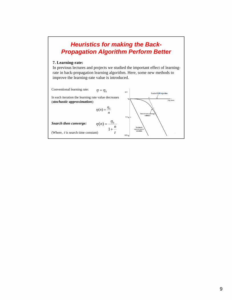
7. Learning-rate:In previous lectures and projects we studied the important effect of learning-rate in back-propagation learning algorithm. Here, some new methods to improve the learning-rate value is introduced.
0 Conventional learning rate:
In each iteration the learning rate value decreases(stochastic approximation):
17
nn 0)(
n
n
1
)( 0Search then converge:
(Where, is search time constant)
1
Artificial Neural NetworksArtificial Neural Networks
Lecture 8
1
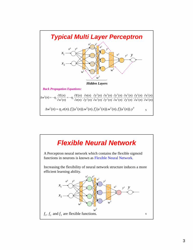
Flexible Neural Networks
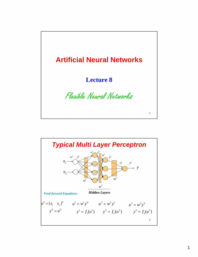
Typical Multi Layer Perceptron
y1x
u1
u3
u0 y0
y1
y3
u2
y2
3w1w
y2x
2w
Hidden LayersFeed-forward Equations:
2
Txxu ][ 210
00 uy
011 ywu
)( 11
1 ufy
122 ywu 2 2
2 ( )y f u
3 3 2u w y3 3
3 ( )y f u
2
Typical Multi Layer Perceptron
y1x
u1
u3
u0 y0
y1
y3
u2
y2
3w1w
2x
2w
Hidden Layers
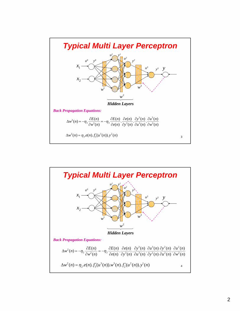
3
Back Propagation Equations:
3 33
3 33 3 3 3
( ) ( ) ( ) ( ) ( )( ) . . .
( ) ( ) ( ) ( ) ( )
E n E n e n y n u nw n
w n e n y n u n w n
3 3 23 3( ) . ( ). ( ( )). ( )w n e n f u n y n
Typical Multi Layer Perceptronu1 y1
y1x u3
u0 y0
y3
u2
y2
Hidden Layers
3w1w
2x
2w
4
Back Propagation Equations:
3 3 2 22
2 22 3 3 2 2 2
( ) ( ) ( ) ( ) ( ) ( ) ( )( ) . . . .
( ) ( ) ( ) ( ) ( ) ( ) ( )
E n E n e n y n u n y n u nw n
w n e n y n u n y n u n w n
2 3 3 2 12 3 2( ) . ( ). ( ( )). ( ). ( ( )). ( )w n e n f u n w n f u n y n
3
Typical Multi Layer Perceptron
y1x
u1
u3
u0 y0
y1
y3
u2
y2
3w1w
2x
2w
Hidden Layers
5
Back Propagation Equations:
3 3 2 2 1 11
1 11 3 3 2 2 1 1 1
( ) ( ) ( ) ( ) ( ) ( ) ( ) ( ) ( )( ) . . . . . . .
( ) ( ) ( ) ( ) ( ) ( ) ( ) ( ) ( )
E n E n e n y n u n y n u n y n u nw n
w n e n y n u n y n u n y n u n w n
1 3 3 2 2 1 01 3 2 1( ) . ( ). ( ( )). ( ). ( ( )). ( ). ( ( )).w n e n f u n w n f u n w n f u n y
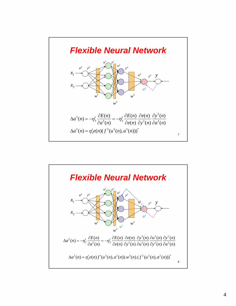
Flexible Neural NetworkA Perceptron neural network which contains the flexible sigmoid functions in neurons is known as Flexible Neural Network.
Increasing the flexibility of neural network structure induces a more efficient learning ability.
y1x
u1
u3
u0 y0
y1
y3
u2
y2
6
3w1w
2x
2w1 2 3, and are flexible functions.f f f
4
Flexible Neural Network
x
u1
u0 y0
y1
u2
y2
3w1w
y1x
2x
u3y3
2w
a3
7
33
3 33 3 3
3 3 3 3 *3
( ) ( ) ( ) ( )( )
( ) ( ) ( ) ( )
( ) ( )( ( ( ), ( )))
E n E n e n y na n
a n e n y n a n
a n e n f u n a n
Flexible Neural Network
x
u1
u0 y0
y1
u2
y2
3w1w
y1x
2x
u3y3
2w
a3
a2
8
3 3 22
2 22 3 3 2 2
( ) ( ) ( ) ( ) ( ) ( )( )
( ) ( ) ( ) ( ) ( ) ( )
E n E n e n y n u n y na n
a n e n y n u n y n a n
2 3 3 3 2 2 2 *2( ) ( ) ( ( ), ( )). ( ).( ( ( ), ( )))a n e n f u n a n w n f u n a n
5
Flexible Neural Network
x
u1
u0 y0
y1
u2
y2
3w1w
y1x
2x
u3y3
2w
a3
9
3 3 2 2 11
1 11 3 3 2 2 1 1
( ) ( ) ( ) ( ) ( ) ( ) ( ) ( )( )
( ) ( ) ( ) ( ) ( ) ( ) ( ) ( )
E n E n e n y n u n y n u n y na n
a n e n y n u n y n u n y n a n
1 3 3 3 2 2 2 1 1 1 *1( ) ( ) ( ( ), ( )). ( ). ( ( ), ( )). ( ).( ( ( ), ( )))a n e n f u n a n w n f u n a n w n f u n a n
A new method to tune the learning-rate
• Delta-bar-Delta– This method is applicable to learning rates in MLP and F.MLP.
( 1) ( 1) ( ) 0
( ) ( 1) ( 1) ( ) 0
0
k k k
k b k k k
Otherwise
10
4 110 10
0.5 0.9b
1
1
Artificial Neural Networks
Lecture 9
Some Applications of Neural Networks (1)(Function Approximation)
2
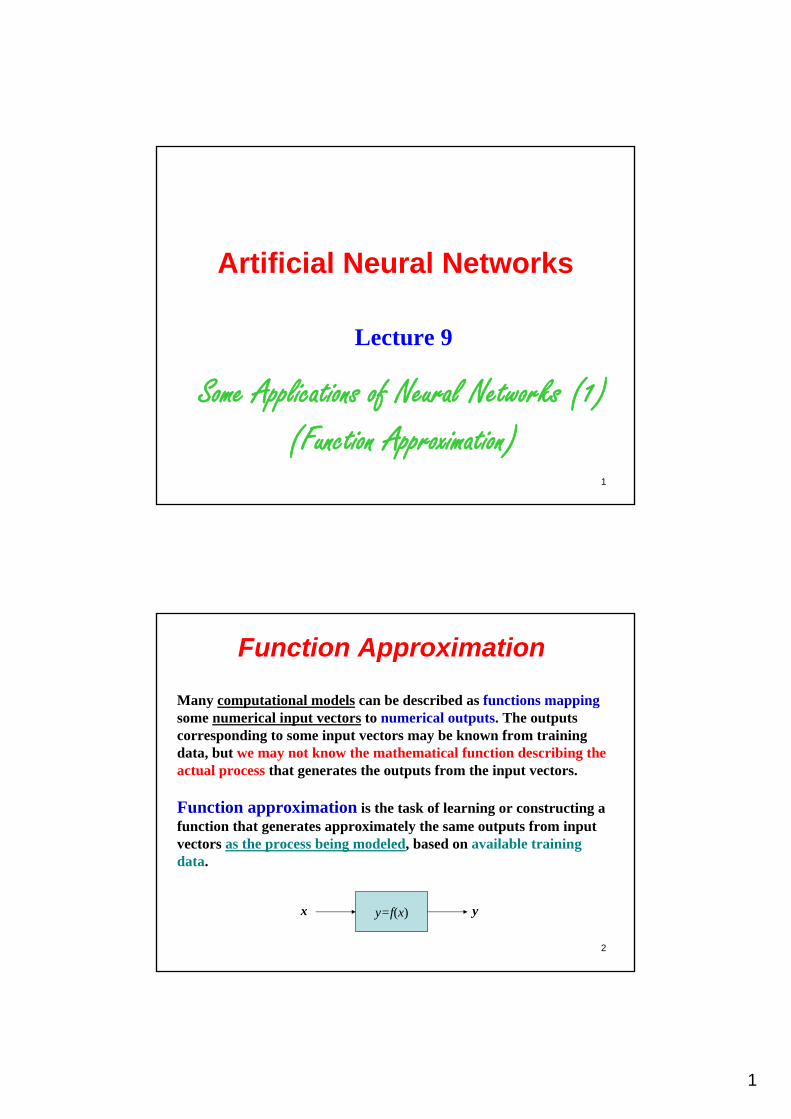
Function Approximation
Many computational models can be described as functions mappingsome numerical input vectors to numerical outputs. The outputs corresponding to some input vectors may be known from training data, but we may not know the mathematical function describing the actual process that generates the outputs from the input vectors.
Function approximation is the task of learning or constructing a function that generates approximately the same outputs from input vectors as the process being modeled, based on available training data.
y=f(x)x y
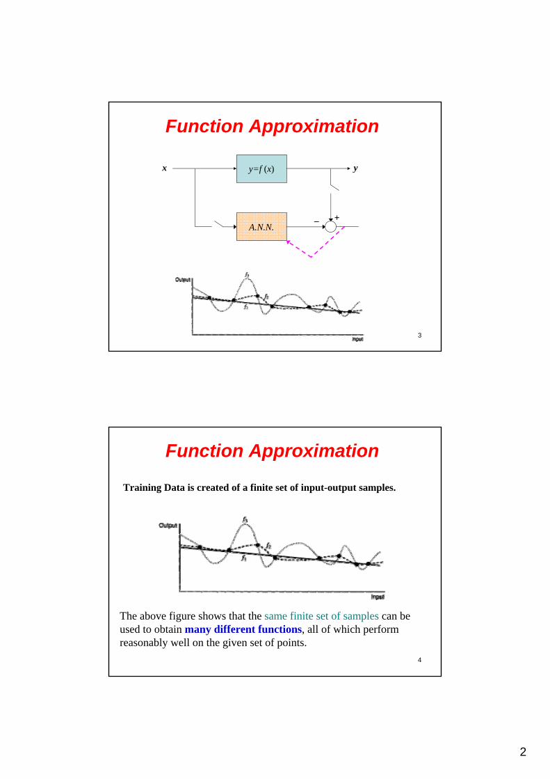
2
3
Function Approximation
y=f (x)x y
A.N.N.+_
4
Function Approximation
Training Data is created of a finite set of input-output samples.
The above figure shows that the same finite set of samples can be used to obtain many different functions, all of which perform reasonably well on the given set of points.
3
5
Function Approximation
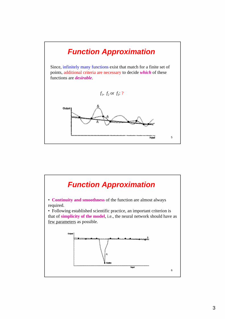
Since, infinitely many functions exist that match for a finite set of points, additional criteria are necessary to decide which of these functions are desirable.
f1, f2 or f3: ?
6
Function Approximation
• Continuity and smoothness of the function are almost always required.• Following established scientific practice, an important criterion is that of simplicity of the model, i.e., the neural network should have as few parameters as possible.
4
7
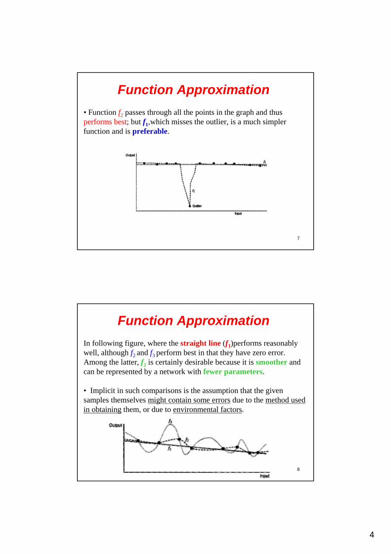
Function Approximation
• Function f2 passes through all the points in the graph and thus performs best; but f1,which misses the outlier, is a much simpler function and is preferable.
8
Function Approximation
In following figure, where the straight line (f1)performs reasonably well, although f2 and f3 perform best in that they have zero error. Among the latter, f2 is certainly desirable because it is smoother and can be represented by a network with fewer parameters.
• Implicit in such comparisons is the assumption that the given samples themselves might contain some errors due to the method used in obtaining them, or due to environmental factors.
5
9
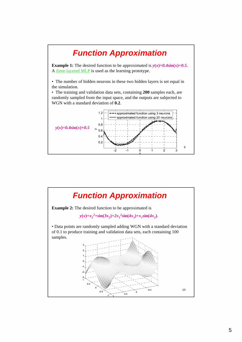
Function ApproximationExample 1: The desired function to be approximated is y(x)=0.4sin(x)+0.5. A three-layered MLP is used as the learning prototype.
• The number of hidden neurons in these two hidden layers is set equal in the simulation. • The training and validation data sets, containing 200 samples each, are randomly sampled from the input space, and the outputs are subjected to WGN with a standard deviation of 0.2.
y(x)=0.4sin(x)+0.5
10
Function ApproximationExample 2: The desired function to be approximated is
y(x)=x22+sin(3x2)+2x1
2sin(4x1)+x1sin(4x2).
• Data points are randomly sampled adding WGN with a standard deviation of 0.1 to produce training and validation data sets, each containing 100 samples.
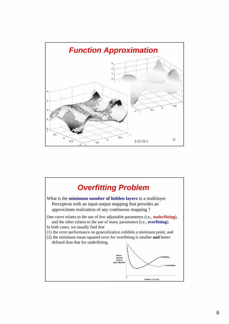
6
11
Function Approximation
2-25-25-1
12
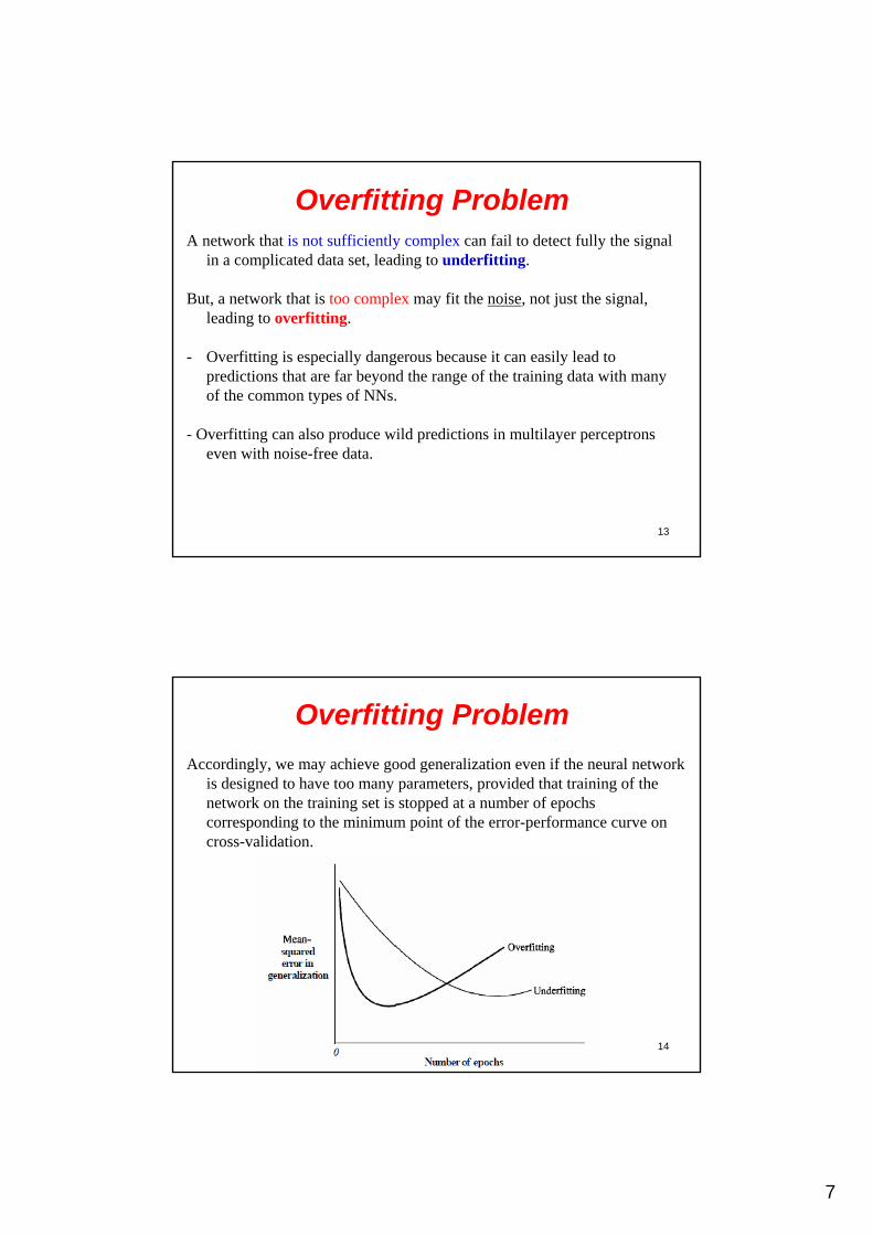
Overfitting ProblemWhat is the minimum number of hidden layers in a multilayer
Perceptron with an input-output mapping that provides an approximate realization of any continuous mapping ?
One curve relates to the use of few adjustable parameters (i.e., underfitting), and the other relates to the use of many parameters (i.e., overfitting).
In both cases, we usually find that (1) the error performance on generalization exhibits a minimum point, and(2) the minimum mean squared error for overfitting is smaller and better
defined than that for underfitting.
7
13
Overfitting ProblemA network that is not sufficiently complex can fail to detect fully the signal
in a complicated data set, leading to underfitting.
But, a network that is too complex may fit the noise, not just the signal, leading to overfitting.
- Overfitting is especially dangerous because it can easily lead to predictions that are far beyond the range of the training data with many of the common types of NNs.
- Overfitting can also produce wild predictions in multilayer perceptrons even with noise-free data.
14
Overfitting Problem
Accordingly, we may achieve good generalization even if the neural network is designed to have too many parameters, provided that training of the network on the training set is stopped at a number of epochs corresponding to the minimum point of the error-performance curve on cross-validation.

8
15
Overfitting Problem
The best way to avoid overfitting is to use lots of training data.
* If you have at least 30 times as many training data as there are weights in the network, you are unlikely to suffer from much overfitting.
* For noise-free data, 5 times as many training data as weights may be sufficient.
* You can't arbitrarily reduce the number of weights due to fear of underfitting.
* Underfitting produces excessive bias in the outputs, whereas overfitting produces excessive variance.
16
3rd Mini Project
By using of an arbitrary neural network (MLP) approximate the function which is presented in example 1.
1st Part of Final ProjectBy using of an arbitrary neural network (MLP) approximate the function
which is presented in example 2. In this project You can use all hints which are introduced in previous lectures
but, you should explain their effects (score: 2 points)
1
1
Artificial Neural Networks
Lecture 10
Some Applications of Neural Networks (2)(System Identification)
2
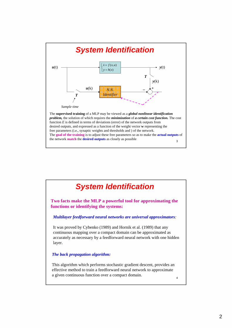
System Identification
The main objective of identification process is to propose specific neural network architectures that can be used for effective identification of a linear/nonlinear system using only input-output data.
Here, the main result is the establishment of input-output models using feedforward neural networks.
u(t) y(t)( ) ( ( ), ( ))
( ) ( ( ))
x t f x t u t
y t h x t
2
3
System Identification
u(t) y(t)
N.N.Identifier
+_
( , )
( )
x f x u
y h x
T
T
Sample time
u(k)
y(k)
The supervised training of a MLP may be viewed as a global nonlinear identification problem, the solution of which requires the minimization of a certain cost function. The cost function E is defined in terms of deviations (error) of the network outputs fromdesired outputs, and expressed as a function of the weight vector w representing thefree parameters (i.e., synaptic weights and thresholds and ) of the network. The goal of the training is to adjust these free parameters so as to make the actual outputs of the network match the desired outputs as closely as possible
4
System Identification
Multilayer feedforward neural networks are universal approximators:
It was proved by Cybenko (1989) and Hornik et al. (1989) that anycontinuous mapping over a compact domain can be approximated as accurately as necessary by a feedforward neural network with one hidden layer.
Two facts make the MLP a powerful tool for approximating the functions or identifying the systems:
The back propagation algorithm:
This algorithm which performs stochastic gradient descent, provides an effective method to train a feedforward neural network to approximatea given continuous function over a compact domain.
3
5
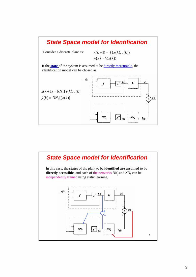
State Space model for Identification
Consider a discrete plant as: ( 1) ( ( ), ( ))
( ) ( ( ))
x k f x k u k
y k h x k
If the state of the system is assumed to be directly measurable, theidentification model can be chosen as:
( 1) [ ( ), ( )]
ˆ( ) [( ( )]
f
h
z k NN z k u k
y k NN x k
6
State Space model for Identification
In this case, the states of the plant to be identified are assumed to be directly accessible, and each of the networks NNf and NNh can be independently trained using static learning.
4
7
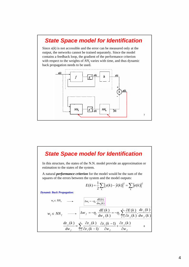
State Space model for IdentificationSince x(k) is not accessible and the error can be measured only at theoutput, the networks cannot be trained separately. Since the model contains a feedback loop, the gradient of the performance criterion with respect to the weights of NNf varies with time, and thus dynamic back propagation needs to be used.
8
State Space model for Identification
In this structure, the states of the N.N. model provide an approximation or estimation to the states of the system.
A natural performance criterion for the model would be the sum of thesquares of the errors between the system and the model outputs:
2 21ˆ( ) ( ) ( ) ( )
2 k k
E k y k y k e k
h hw NN ( )
( )h hh
dE kw
dw k
f fw NN1
( )( ) ( ).
( ) ( ) ( )
nj
f f fjf j f
dz kdE k E kw
dw k z k dw k
1
( ) ( ) ( )( 1).
( 1)
nj j jl
lf l f f
dz k z k z kz k
dw z k w w
Dynamic Back Propagation:
5
9
State Space model for Identification
• Training was done with a random input uniformly distributed in [—1,1].
• The identification model was tested with sinusoidal inputs
1 2
2 1 2
2
1 2
( 1) ( ) 1 0.2 ( )
( 1) 0.2 ( ) 0.5 ( ) ( )
( ) 0.3 ( ) 2 ( )
x k x k u k
x k x k x k u k
y k x k x k
Example 1:
1 1 1 2
1 2 1 2
1 2
ˆ ˆ ˆ( 1) ( ), ( ), ( )
ˆ ˆ ˆ( 1) ( ), ( ), ( )
ˆ ˆ ˆ( ) ( ), ( )
f
f
h
x k NN x k x k u k
x k NN x k x k u k
y k NN x k x k
10
Input-Output model for Identification
Clearly, choosing the state space models for identification requires the use ofdynamic back propagation, which is computationally a very intensive procedure.
At the same time, to avoid instabilities while training, one needs to use small learning rate to adjust the parameters, and this in turn results in long convergence times.
Consider the difference Equation corresponding to a typical linear plant:
1
1 1
( ) ( ) ( )n n
i ji j
y k a y k i b u k j
Input-Output Model of plant:
6
11
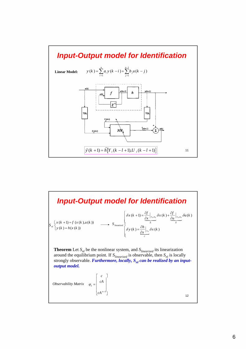
Input-Output model for Identification1
1 1
( ) ( ) ( )n n
i ji j
y k a y k i b u k j
( 1) ( 1), ( 1)l ly k h Y k l U k l
Linear Model:
12
Input-Output model for Identification
( 1) ( ( ), ( ))
( ) ( ( ))nl
x k f x k u kS
y k h x k
0 0 0 0
0
, ,( 1) ( ) ( )
( ) ( )
x u x u
A blinearized
x
c
f fx k x k u k
x u
Sh
y k x kx
Theorem Let Snl be the nonlinear system, and Slinearized its linearization around the equilibrium point. If Slinearized is observable, then Snl is locally strongly observable. Furthermore, locally, Snl can be realized by an input-output model.
1
o
n
c
cA
cA
Observability Matrix
7
13
Input-Output model for Identification
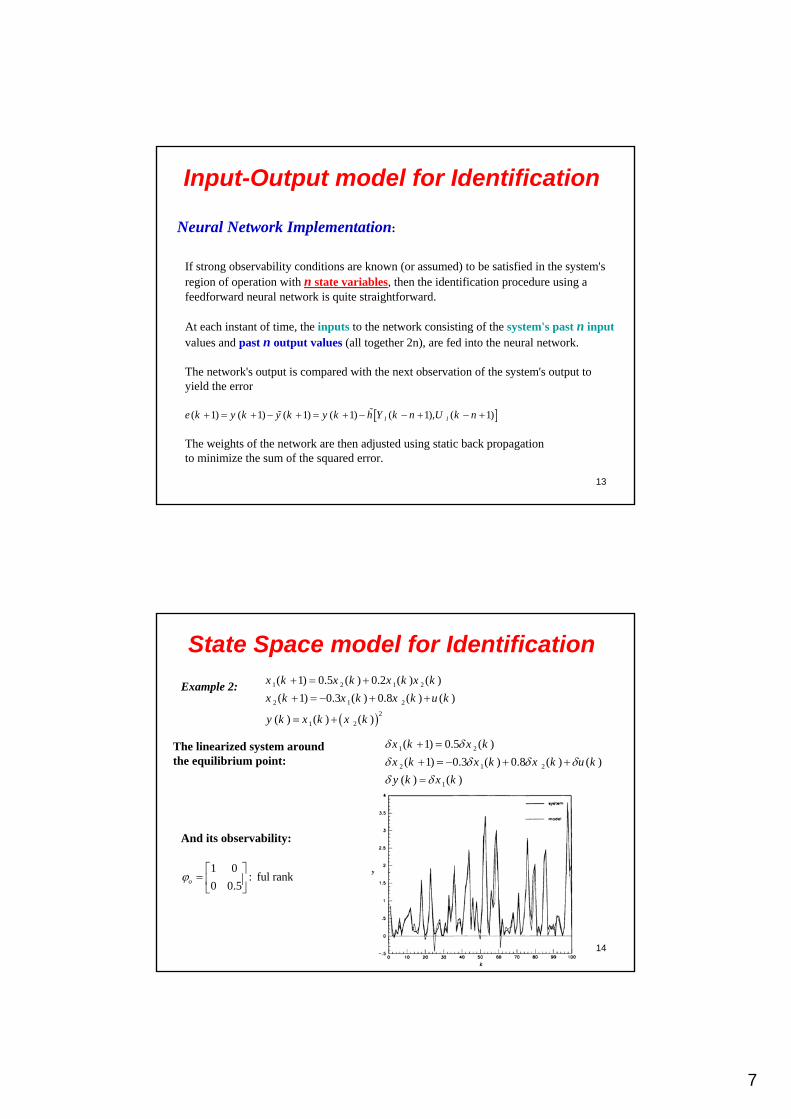
If strong observability conditions are known (or assumed) to be satisfied in the system's region of operation with n state variables, then the identification procedure using a feedforward neural network is quite straightforward.
At each instant of time, the inputs to the network consisting of the system's past n inputvalues and past n output values (all together 2n), are fed into the neural network.
The network's output is compared with the next observation of the system's output toyield the error
The weights of the network are then adjusted using static back propagationto minimize the sum of the squared error.
Neural Network Implementation:
( 1) ( 1) ( 1) ( 1) ( 1), ( 1)l le k y k y k y k h Y k n U k n
14
State Space model for Identification
1 2 1 2
2 1 2
2
1 2
( 1) 0.5 ( ) 0.2 ( ) ( )
( 1) 0.3 ( ) 0.8 ( ) ( )
( ) ( ) ( )
x k x k x k x k
x k x k x k u k
y k x k x k
Example 2:
The linearized system around the equilibrium point:
1 2
2 1 2
1
( 1) 0.5 ( )
( 1) 0.3 ( ) 0.8 ( ) ( )
( ) ( )
x k x k
x k x k x k u k
y k x k
And its observability:
1 0: ful rank
0 0.5o
8
15
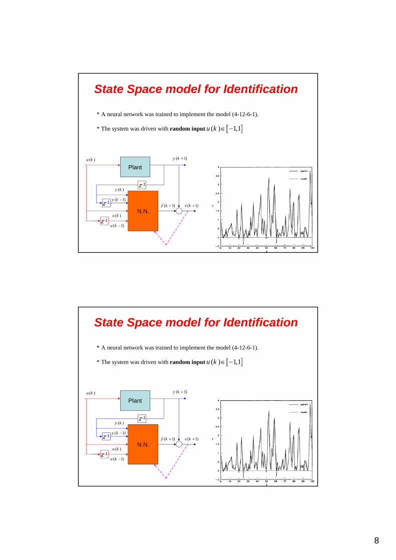
State Space model for Identification
* A neural network was trained to implement the model (4-12-6-1).
* The system was driven with random input ( ) 1,1u k
Plant
N.N.z-1
z-1
z-1
( 1)y k
ˆ ( 1)y k ( 1)e k
( )y k
( 1)y k
( )u k
( 1)u k
( )u k
16
State Space model for Identification
* A neural network was trained to implement the model (4-12-6-1).
* The system was driven with random input ( ) 1,1u k
Plant
N.N.z-1
z-1
z-1
( 1)y k
ˆ ( 1)y k ( 1)e k
( )y k
( 1)y k
( )u k
( 1)u k
( )u k

9
17
2nd Part of Final Project
By using of an arbitrary neural network (MLP) identify the discrete nonlinear plant which is presented in example 2 (Score: 1 points).
• By using a test signal, show that the N.N. identifier perform a appropriate input-output model of plant.
• By using of the PRBS signal, repeat the identifying procedure and compare the results.
The material of this lecture is based on:
Omid Omidvar and David L. Elliott, Neural Systems for Control, Academic Press; 1st edition (1997).
1
Artificial Neural Networks
Lecture 11
Some Applications of Neural Networks (3)(Control)
2
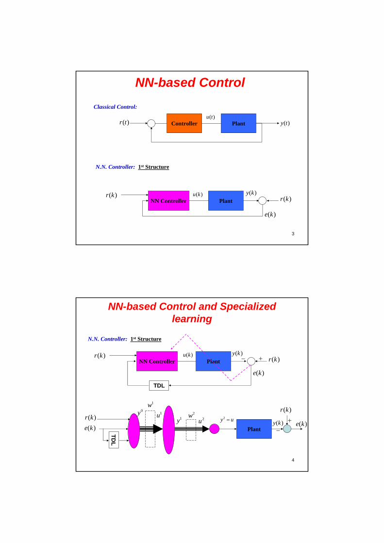
NN-based Control
One of the most important applications of N.N. is its employment in control theory.
In most cases, the ordinary control theory cannot be easily applied, due to the presence of uncertainty, nonlinearity or time varying parameters in real plants.N.N. can overcome these problems with interesting properties such as parallel processing, flexibility in structure and real time learning.
Generally, the NN-based control is called neuromorphic control
3
NN-based Control
Classical Control:
Controller Plant( )r t ( )y t( )u t
N.N. Controller: 1st Structure
NN Controller Plant ( )r k( )y k( )u k( )r k
( )e k
4
NN-based Control and Specialized learning
N.N. Controller: 1st Structure
NN Controller Plant ( )r k( )y k( )u k( )r k
( )e k
TDL
( )r k
( )e k
1w2w
0y 1u1y 2u
2y u
Plant
( )r k
( )y k ( )e k
TD
L
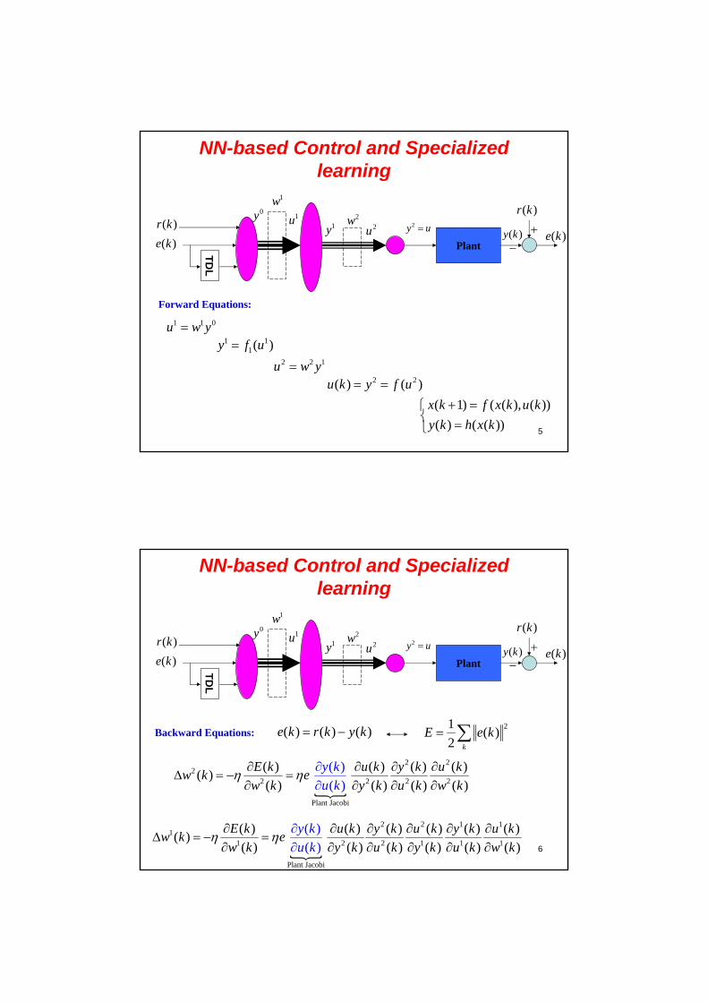
5
NN-based Control and Specialized learning
( )r k
( )e k
1w2w
0y 1u1y 2u
2y u
Plant
( )r k
( )y k ( )e k
TD
L
Forward Equations:
1 1 0u w y1 1
1( )y f u2 2 1u w y
2 2( ) ( )u k y f u ( 1) ( ( ), ( ))
( ) ( ( ))
x k f x k u k
y k h x k
6
NN-based Control and Specialized learning
( )r k
( )e k
1w2w
0y 1u1y 2u
2y u
Plant
( )r k
( )y k ( )e k
TD
L
Backward Equations: ( ) ( ) ( )e k r k y k
2 22
2 2 2 2
Plant Jacobi
( ) ( ) ( ) ( )( )
( ) ( ) (
( )
( ) () )
E k u k y k u kw k e
w k y
y k
u k w kk k u
21( )
2 k
E e k
2 2 1 11
1 2 2 1 1 1
Plant Jacobi
( ) ( ) ( ) ( ) ( ) ( )( )
( ) ( ) ( ) ( ) ( ) (
( )
( ) )
E k u k y k u ky k y k u kw k e
w k y k u k y k uk ku w k
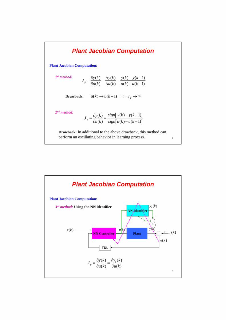
7
Plant Jacobian Computation
Plant Jacobian Computation:
( ) ( ) ( ) ( 1)
( ) ( ) ( ) ( 1)p
y k y k y k y kJ
u k u k u k u k
1st method:
Drawback: ( ) ( 1) pu k u k J
2nd method:
( ) ( 1)( )
( ) ( ) ( 1)p
sign y k y ky kJ
u k sign u k u k
Drawback: In additional to the above drawback, this method can perform an oscillating behavior in learning process.
8
Plant Jacobian Computation
Plant Jacobian Computation:
3rd method: Using the NN identifier
( )( )
( ) ( )I
p
y ky kJ
u k u k
NN Controller Plant ( )r k( )y k( )u k( )r k
( )e k
TDL
NN Identifier
( )Iy k
9
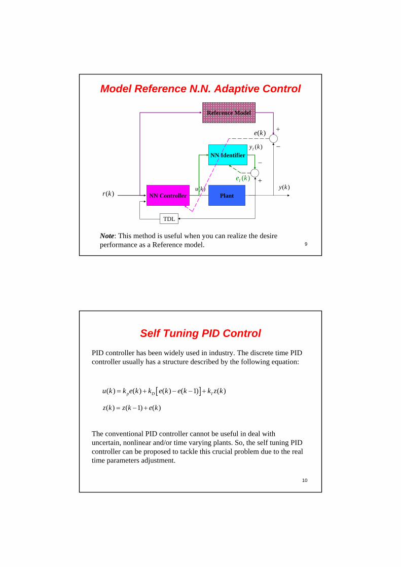
Model Reference N.N. Adaptive Control
Note: This method is useful when you can realize the desire performance as a Reference model.
NN Controller Plant
( )y k( )u k( )r k
( )e k
NN Identifier
( )Iy k
Reference Model
( )Ie k
TDL
10
Self Tuning PID Control
( ) ( ) ( ) ( 1) ( )p D Iu k k e k k e k e k k z k
PID controller has been widely used in industry. The discrete time PID controller usually has a structure described by the following equation:
( ) ( 1) ( )z k z k e k
The conventional PID controller cannot be useful in deal with uncertain, nonlinear and/or time varying plants. So, the self tuning PID controller can be proposed to tackle this crucial problem due to the real time parameters adjustment.
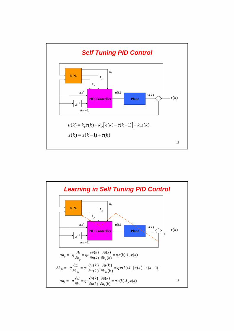
11
Self Tuning PID Control
( ) ( ) ( ) ( 1) ( )p D Iu k k e k k e k e k k z k
( ) ( 1) ( )z k z k e k
PID Controller Plant( )y k
( )u k
N.N.
1z
( )e k
( 1)e k
pk
Ik
Dk
( )r k
12
Learning in Self Tuning PID Control
( ) ( ). . ( ). . ( )
( ) ( )p pp p
E y k u kk e e k J e k
k u k k k
( ) ( ). . ( ). . ( ) ( 1)
( ) ( )D pD D
E y k u kk e e k J e k e k
k u k k k
PID Controller Plant( )y k
( )u k
N.N.
1z
( )e k
( 1)e k
pk
Ik
Dk
( )r k
( ) ( ). . ( ). . ( )
( ) ( )I pI I
E y k u kk e e k J z k
k u k k k
13
Self Tuning PID Control
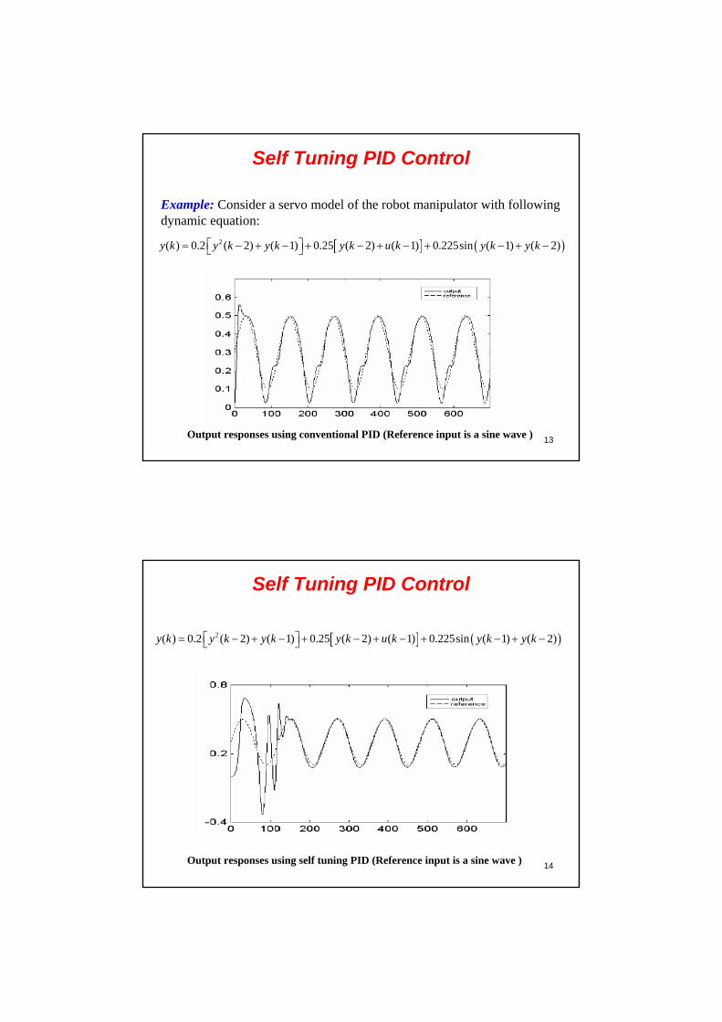
Example: Consider a servo model of the robot manipulator with following dynamic equation:
2( ) 0.2 ( 2) ( 1) 0.25 ( 2) ( 1) 0.225sin ( 1) ( 2)y k y k y k y k u k y k y k
Output responses using conventional PID (Reference input is a sine wave )
14
Self Tuning PID Control
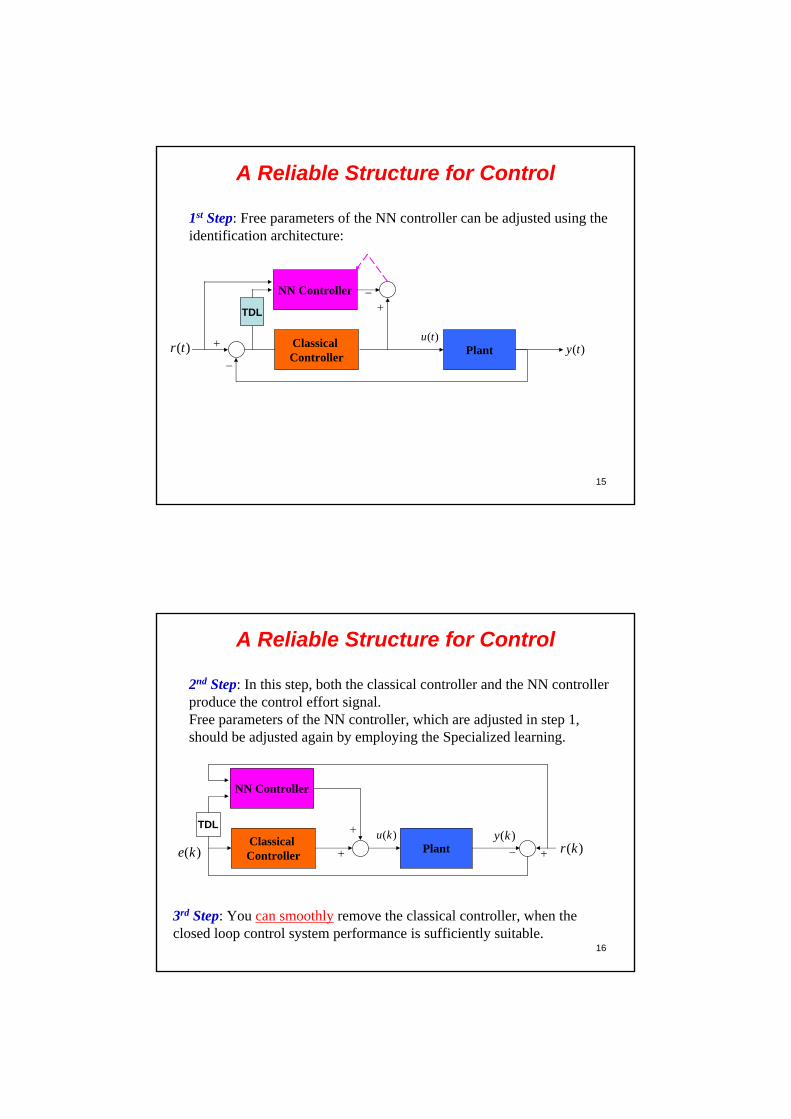
2( ) 0.2 ( 2) ( 1) 0.25 ( 2) ( 1) 0.225sin ( 1) ( 2)y k y k y k y k u k y k y k
Output responses using self tuning PID (Reference input is a sine wave )
15
A Reliable Structure for Control
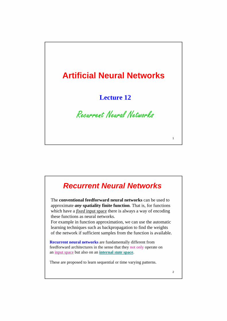
1st Step: Free parameters of the NN controller can be adjusted using theidentification architecture:
Classical Controller
Plant( )r t ( )y t( )u t
NN Controller
TDL
16
A Reliable Structure for Control
2nd Step: In this step, both the classical controller and the NN controller produce the control effort signal.Free parameters of the NN controller, which are adjusted in step 1, should be adjusted again by employing the Specialized learning.
Classical Controller
Plant ( )r k( )y k( )u k
NN Controller
( )e k
TDL
3rd Step: You can smoothly remove the classical controller, when the closed loop control system performance is sufficiently suitable.

17
3rd Part of Final Project
In this project, you should find a practical plant in papers and by using of NN controllers provide a suitable closed loop control performance. (Score: 2 points)
• In this project you can use of any NN controllers structure which are presented in this lecture.
• In this project you can use of any NN controllers which are introduced in papers and text books (score: +1 point).
18
Literature Cited
The material of this lecture is based on:
[1] M. Teshnehlab, K. Watanabe, Intelligent Control based on Flexible Neural Network, Springer; 1 edition, 1999.
[2] Woo-yong Han, Jin-wook Han, Chang-goo Lee, Development of a Self-tuning PID Controller based on Neural Network for Nonlinear Systems, In: Proc. of the 7th Mediterranean Conference on Control and Automation (MED99) June 28-30, 1999.
1
Artificial Neural Networks
Lecture 12
Recurrent Neural Networks
2
Recurrent Neural Networks
The conventional feedforward neural networks can be used to approximate any spatiality finite function. That is, for functions which have a fixed input space there is always a way of encoding these functions as neural networks. For example in function approximation, we can use the automatic learning techniques such as backpropagation to find the weights of the network if sufficient samples from the function is available.
Recurrent neural networks are fundamentally different from feedforward architectures in the sense that they not only operate on an input space but also on an internal state space.
These are proposed to learn sequential or time varying patterns.
3
Recurrent Neural Networks
Recurrent Neural Networks, unlike the feed-forward neural networks, contain the feedback connections among the neurons.
Three subsets of neurons are presented in the recurrent networks:
1. Input neurons2. Output neurons3. Hidden neurons, which are neither input nor output neurons.
Note that a neuron can be simultaneously an input and output neuron; such neurons are said to be autoassociative.
Recurrent Neural Networks
4
5
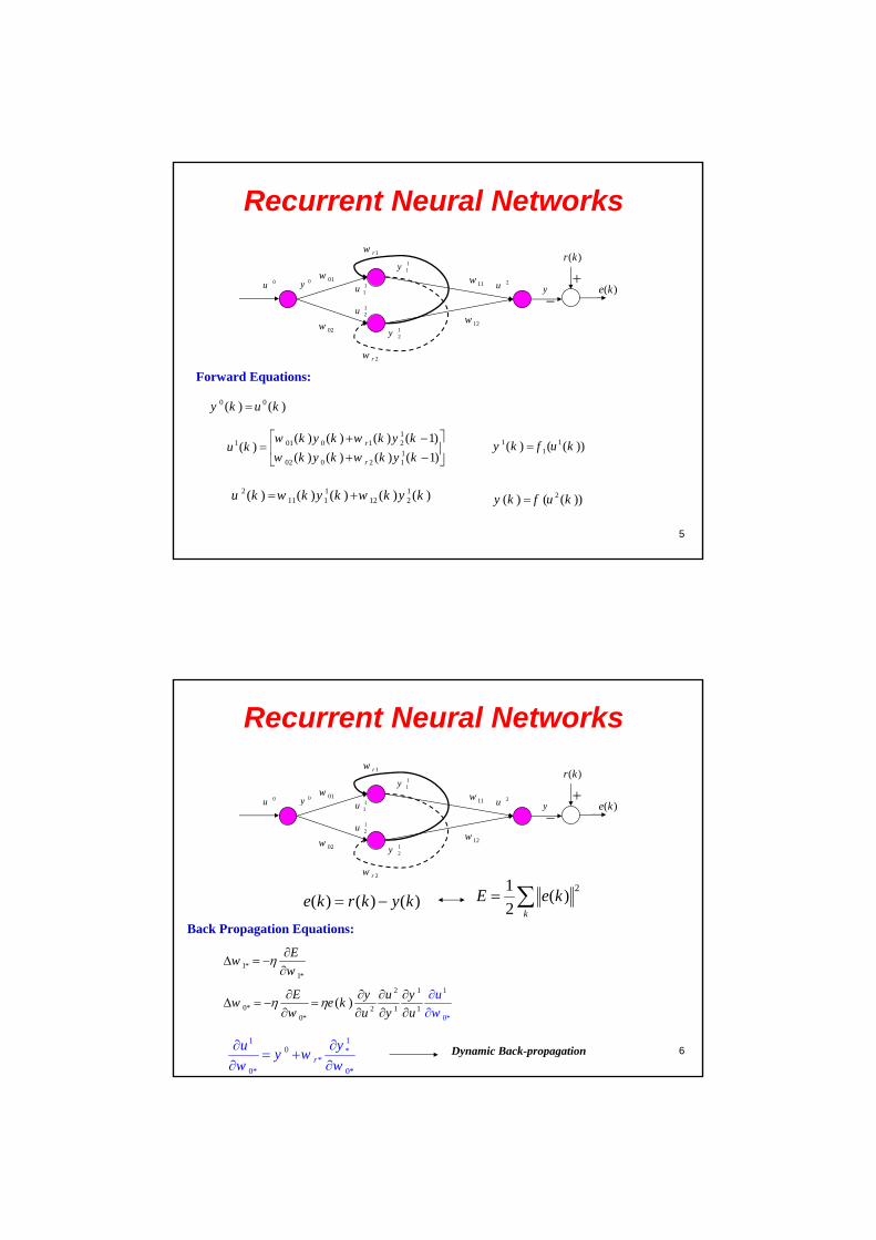
Recurrent Neural Networks
0y
( )r k
( )e k0u
01w
02w
1rw
2rw
11y
12y
11u
12u
11w
12w
2u y
Forward Equations:
11 01 0 1 2
102 0 2 1
( ) ( ) ( ) ( 1)( )
( ) ( ) ( ) ( 1)r
r
w k y k w k y ku k
w k y k w k y k
2 1 111 1 12 2( ) ( ) ( ) ( ) ( )u k w k y k w k y k 2( ) ( ( ))y k f u k
0 0( ) ( )y k u k
1 11( ) ( ( ))y k f u k
6
Recurrent Neural Networks
0y
( )r k
( )e k0u
01w
02w
1rw
2rw
11y
12y
11u
12u
11w
12w
2u y
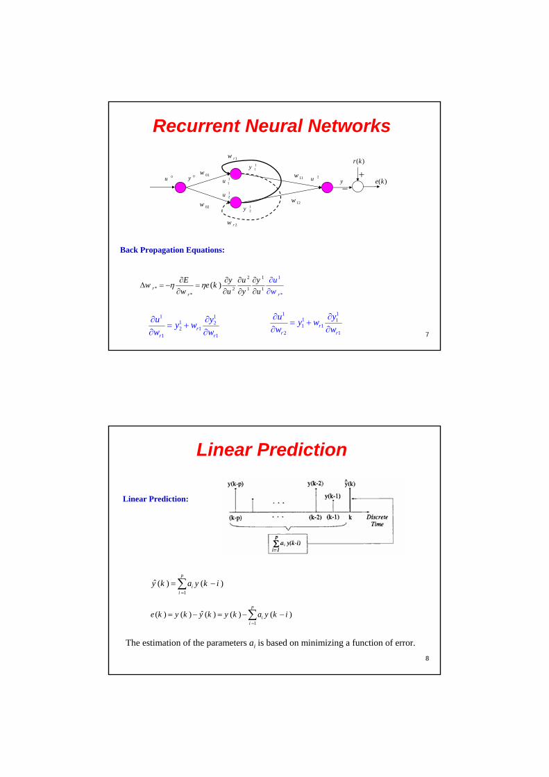
Back Propagation Equations:
1*1*
Ew
w
( ) ( ) ( )e k r k y k 21
( )2 k
E e k
2 1
0* 2 1 10*
1
0*
( )E y u y
w e kw u u
u
y w
110 *
*0* 0*
r
yuy w
w w
Dynamic Back-propagation
7
Recurrent Neural Networks
0y
( )r k
( )e k0u
01w
02w
1rw
2rw
11y
12y
11u
12u
11w
12w
2u y
Back Propagation Equations:
2 1
* 2 1 1*
1
*
( )rr r
E y u yw e k
w u u
u
y w
111 22 1
1 1r
r r
yuy w
w w
111 11 1
2 1r
r r
yuy w
w w
8
Linear Prediction
Linear Prediction:
1
ˆ ( ) ( )p
ii
y k a y k i
1
ˆ( ) ( ) ( ) ( ) ( )p
ii
e k y k y k y k a y k i
The estimation of the parameters ai is based on minimizing a function of error.
9
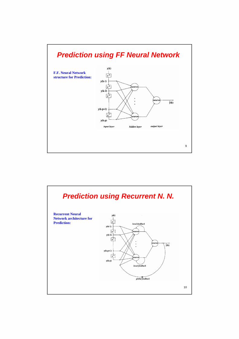
Prediction using FF Neural Network
F.F. Neural Network structure for Prediction:
10
Prediction using Recurrent N. N.
Recurrent Neural Network architecture for Prediction:
11
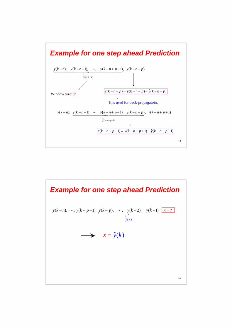
Example for one step ahead Prediction
ˆ ( )
( ), ( 1), , ( 1) , ( )
y k n p
y k n y k n y k n p y k n p
ˆ( ) ( ) ( )e k n p y k n p y k n p
It is used for back-propagatoin.
ˆ ( 1)
( ), ( 1) ( 1) ( ) , ( 1)
y k n p
y k n y k n y k n p y k n p y k n p
ˆ( 1) ( 1) ( 1)e k n p y k n p y k n p
Window size: P
12
Example for one step ahead Prediction
ˆ( )
( ), , ( 1), ( ), , ( 2), ( 1) ?
y k
xy k n y k p y k p y k y k
ˆ( )x y k
13
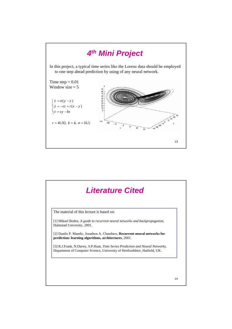
4th Mini Project
In this project, a typical time series like the Lorenz data should be employed to one step ahead prediction by using of any neural network.
Time step = 0.01Window size = 5
( )
( )
45.92, 4, 16.5
x y x
y xz r x y
z xy bz
r b
14
Literature Cited
The material of this lecture is based on:
[1] Mikael Boden. A guide to recurrent neural networks and backpropagation, Halmstad University, 2001.
[2] Danilo P. Mandic, Jonathon A. Chambers, Recurrent neural networks for prediction: learning algorithms, architectures, 2001.
[3] R.J.Frank, N.Davey, S.P.Hunt, Time Series Prediction and Neural Networks, Department of Computer Science, University of Hertfordshire, Hatfield, UK.
1
Artificial Neural Networks
Lecture 13
RBF Networks
2
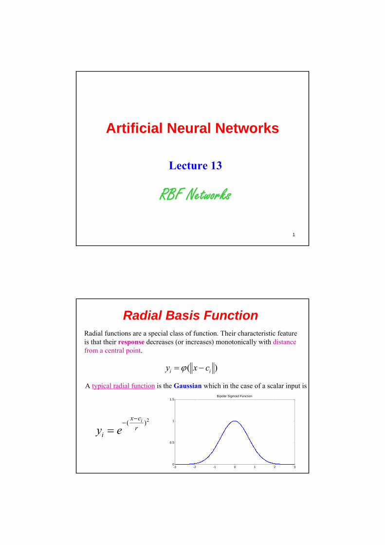
Radial Basis FunctionRadial functions are a special class of function. Their characteristic feature is that their response decreases (or increases) monotonically with distance from a central point.
( )i iy x c
A typical radial function is the Gaussian which in the case of a scalar input is
2( )ix c
riy e
-3 -2 -1 0 1 2 30
0.5
1
1.5Bipolar Sigmoid Function
3
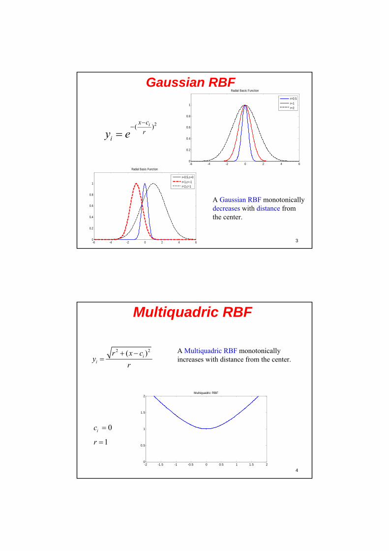
Gaussian RBF
2( )ix c
riy e
-6 -4 -2 0 2 4 60
0.2
0.4
0.6
0.8
1
Radial Basis Function
r=0.5
r=1r=2
A Gaussian RBF monotonically decreases with distance from the center.
-6 -4 -2 0 2 4 60
0.2
0.4
0.6
0.8
1
Radial Basis Function
r=0.5,c=0
r=1,c=-1r=2,c=1
4
Multiquadric RBF
2 2( )ii
r x cy
r
A Multiquadric RBF monotonically increases with distance from the center.
-2 -1.5 -1 -0.5 0 0.5 1 1.5 20
0.5
1
1.5
2Multiquadric RBF
0ic
1r
5
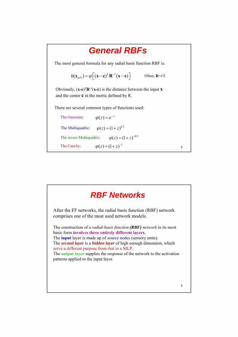
General RBFsThe most general formula for any radial basis function RBF is:
1*1( ) ( ) ( )T
mh x x c R x c
Obviously, (x-c)TR-1(x-c) is the distance between the input xand the center c in the metric defined by R.
There are several common types of functions used:
The Gaussian: ( ) zz e
The Multiquadric: 0.5( ) (1 )z z
The Cauchy:
The invers Multiquadric: 0.5( ) (1 )z z 1( ) (1 )z z
Often, R=r2I.
6
RBF Networks
After the FF networks, the radial basis function (RBF) network comprises one of the most used network models.
The construction of a radial-basis function (RBF) network in its most basic form involves three entirely different layers. The input layer is made up of source nodes (sensory units). The second layer is a hidden layer of high enough dimension, which serve a different purpose from that in a MLP. The output layer supplies the response of the network to the activation patterns applied to the input layer.
7
RBF Networks
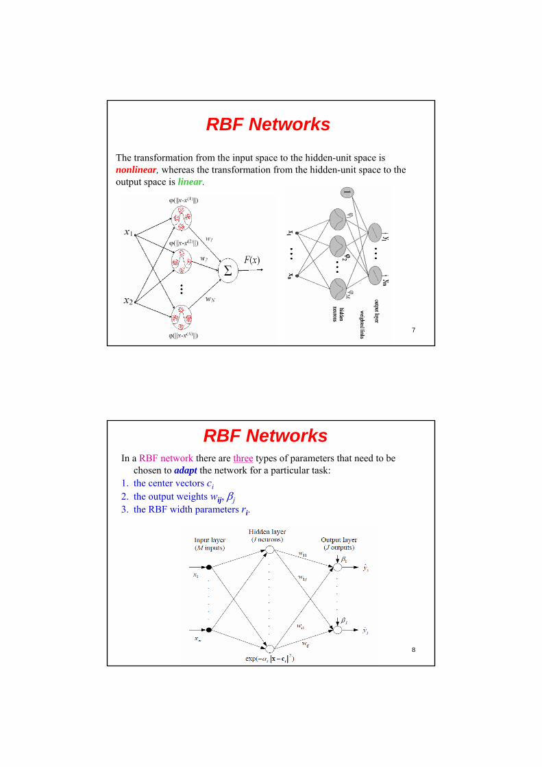
The transformation from the input space to the hidden-unit space is nonlinear, whereas the transformation from the hidden-unit space to the output space is linear.
8
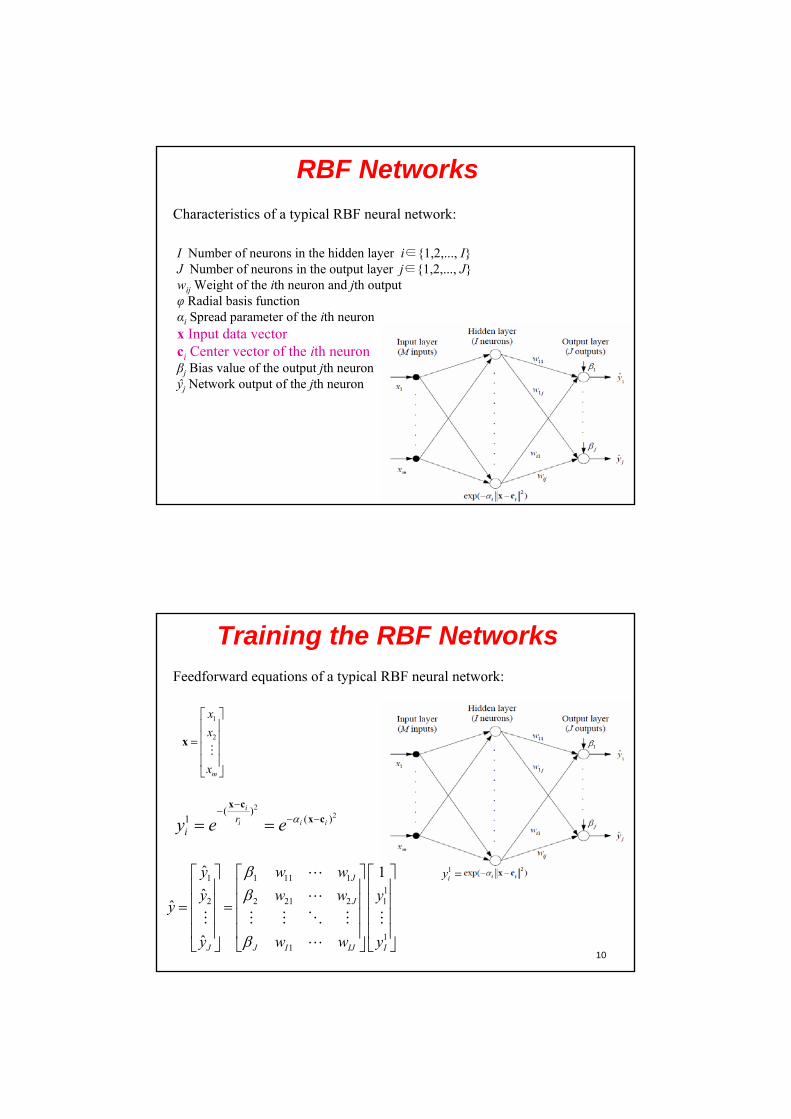
RBF NetworksIn a RBF network there are three types of parameters that need to be
chosen to adapt the network for a particular task: 1. the center vectors ci
2. the output weights wij, j
3. the RBF width parameters ri.
9
RBF Networks
Characteristics of a typical RBF neural network:
I Number of neurons in the hidden layer i∈{1,2,..., I}J Number of neurons in the output layer j∈{1,2,..., J}wij Weight of the ith neuron and jth outputφ Radial basis functionαi Spread parameter of the ith neuronx Input data vectorci Center vector of the ith neuronβj Bias value of the output jth neuronŷj Network output of the jth neuron
10
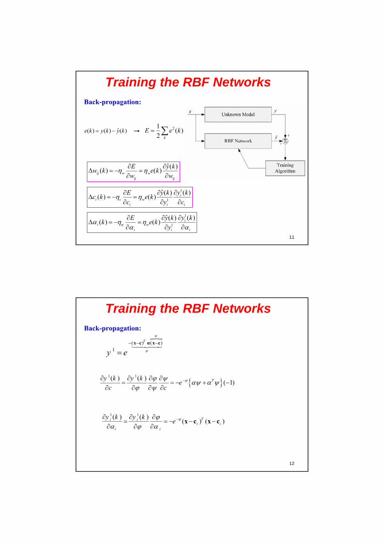
Training the RBF NetworksFeedforward equations of a typical RBF neural network:
1
2
m
x
x
x
x
1iy
22( )
( )1i
i i iriy e e
x c
x c
1 1 11 11
2 2 21 2 1
11
ˆ 1
ˆˆ
ˆ
J
J
J J I IJ I
y w w
y w w yy
y w w y
11
Training the RBF NetworksBack-propagation:
ˆ( ) ( ) ( )e k y k y k 21( )
2 k
E e k
ˆ( )( ) ( )ij w w
ij ij
E y kw k e k
w w
1
1
ˆ ( )( )( ) ( ) i
i c wi i i
y kE y kc k e k
c y c
1
1
ˆ ( )( )( ) ( ) i
i wi i i
y kE y kk e k
y
12
Training the RBF NetworksBack-propagation:
1 1( ) ( )
( 1)Ty k y ke
c c
( ) ( )
1
T
y e
x c α x c
1 1( ) ( )( ) ( )Ti i
i ii i
y k y ke
x c x c
13
Comparison of RBF Networks and MLP [1]
Radial-basis function (RBF) networks and multilayer perceptrons are examples of nonlinear layered feedforward networks. They are both universal approximators.
However, these two networks differ from each other in several important respects, as:
1. An RBF network (in its most basic form) has a single hidden layer, whereas an MLP may have one or more hidden layers.
2. Typically, the computation nodes of an MLP, be they located in a hidden or output layer, share a common neuron model. On the other hand, the computation nodes in the hidden layer of an RBF network are quite different and serve a different purpose from those in the output layer of the network.
14
Comparison of RBF Networks and MLP [1]
3. The hidden layer of an RBF network is nonlinear, whereas the output layer is linear. On the other hand, the hidden and output layers of an MLP used as a classifier are usually all nonlinear; however, when the MLP is used to solve nonlinear regression problems, a linear layer for the output is usually the preferred choice.
4. The argument of the activation function of each hidden unit in an RBF network computes the Euclidean norm (distance) between the input vector and the center of that unit. On the other hand, the activation function of each hidden unit in an MLP computes the inner product of the input vector and the synaptic weight vector of that unit.
15
Comparison of RBF Networks and MLP [1]
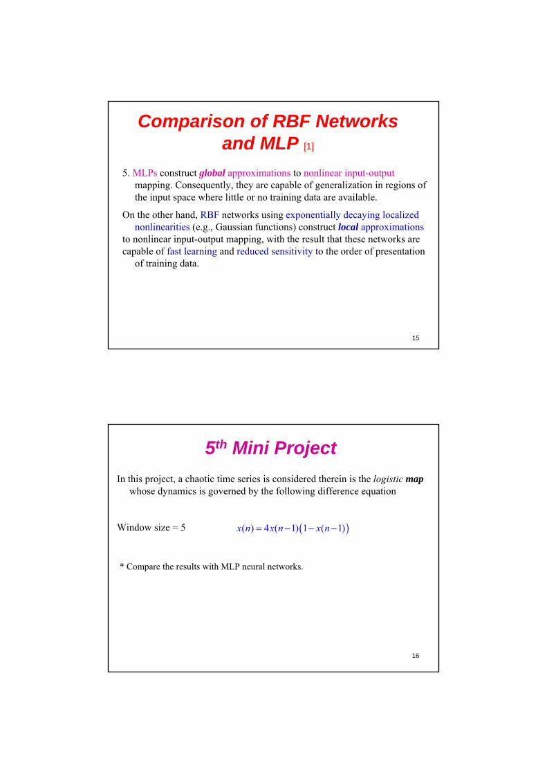
5. MLPs construct global approximations to nonlinear input-outputmapping. Consequently, they are capable of generalization in regions of the input space where little or no training data are available.
On the other hand, RBF networks using exponentially decaying localized nonlinearities (e.g., Gaussian functions) construct local approximations
to nonlinear input-output mapping, with the result that these networks arecapable of fast learning and reduced sensitivity to the order of presentation
of training data.
16
5th Mini Project
In this project, a chaotic time series is considered therein is the logistic map whose dynamics is governed by the following difference equation
Window size = 5 ( ) 4 ( 1) 1 ( 1)x n x n x n
* Compare the results with MLP neural networks.
17
Literature Cited
The material of this lecture is based on:
[1] Simon Haykin, Neural Networks: A Comprehensive Foundation., Prentice Hall, 1998.
[2] Tuba Kurban and Erkan Beşdok, A Comparison of RBF Neural Network Training Algorithms for Inertial Sensor Based Terrain Classification., Sensors, 9, 6312-6329; (doi:10.3390/s90806312), 2009.
[3] Mark J. L. Orr, Introduction to Radial Basis Function Networks, Centre for Cognitive Science, University of Edinburgh, 1996.
1
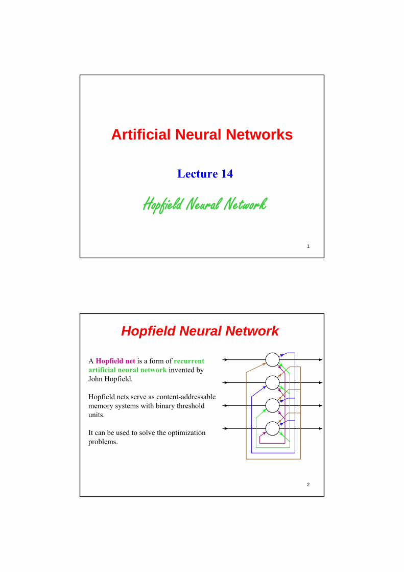
Artificial Neural Networks
Lecture 14
Hopfield Neural Network
2
Hopfield Neural Network
A Hopfield net is a form of recurrent artificial neural network invented by John Hopfield.
Hopfield nets serve as content-addressable memory systems with binary thresholdunits.
It can be used to solve the optimization problems.
3
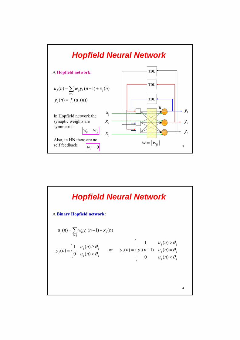
Hopfield Neural Network
A Hopfield network:
( ) ( 1) ( )j ij i ji j
u n w y n x n
( ) ( ( ))j j jy n f u n TDL
TDL
TDL
1x 1y
2y
3y
[ ]ijw w
2x
3x
u
ij jiw w
In Hopfield network the synaptic weights are symmetric:
0iiw
Also, in HN there are no self feedback:
4
Hopfield Neural Network
A Binary Hopfield network:
( ) ( 1) ( )j ij i ji j
u n w y n x n
1 ( )( )
0 ( )j j
jj j
u ny n
u n
1 ( )
or ( ) ( 1) ( )
0 ( )
j j
j j j j
j j
u n
y n y n u n
u n
5
Hopfield Neural Network
The energy E for the whole network can be determined from energy function as the following equation:
1
2 ij i j i i i ii j i i
E w y y x y y
i ij j i i ij
E w y x y
So:
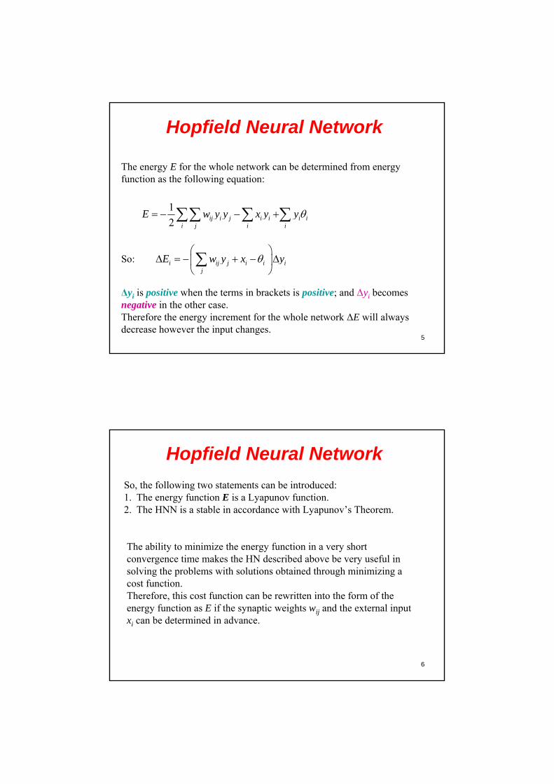
Δyi is positive when the terms in brackets is positive; and Δyi becomes negative in the other case. Therefore the energy increment for the whole network ΔE will always decrease however the input changes.
6
Hopfield Neural Network
The ability to minimize the energy function in a very short convergence time makes the HN described above be very useful in solving the problems with solutions obtained through minimizing a cost function. Therefore, this cost function can be rewritten into the form of the energy function as E if the synaptic weights wij and the external input xi can be determined in advance.
So, the following two statements can be introduced:1. The energy function E is a Lyapunov function.2. The HNN is a stable in accordance with Lyapunov’s Theorem.
7
Hopfield Neural Network
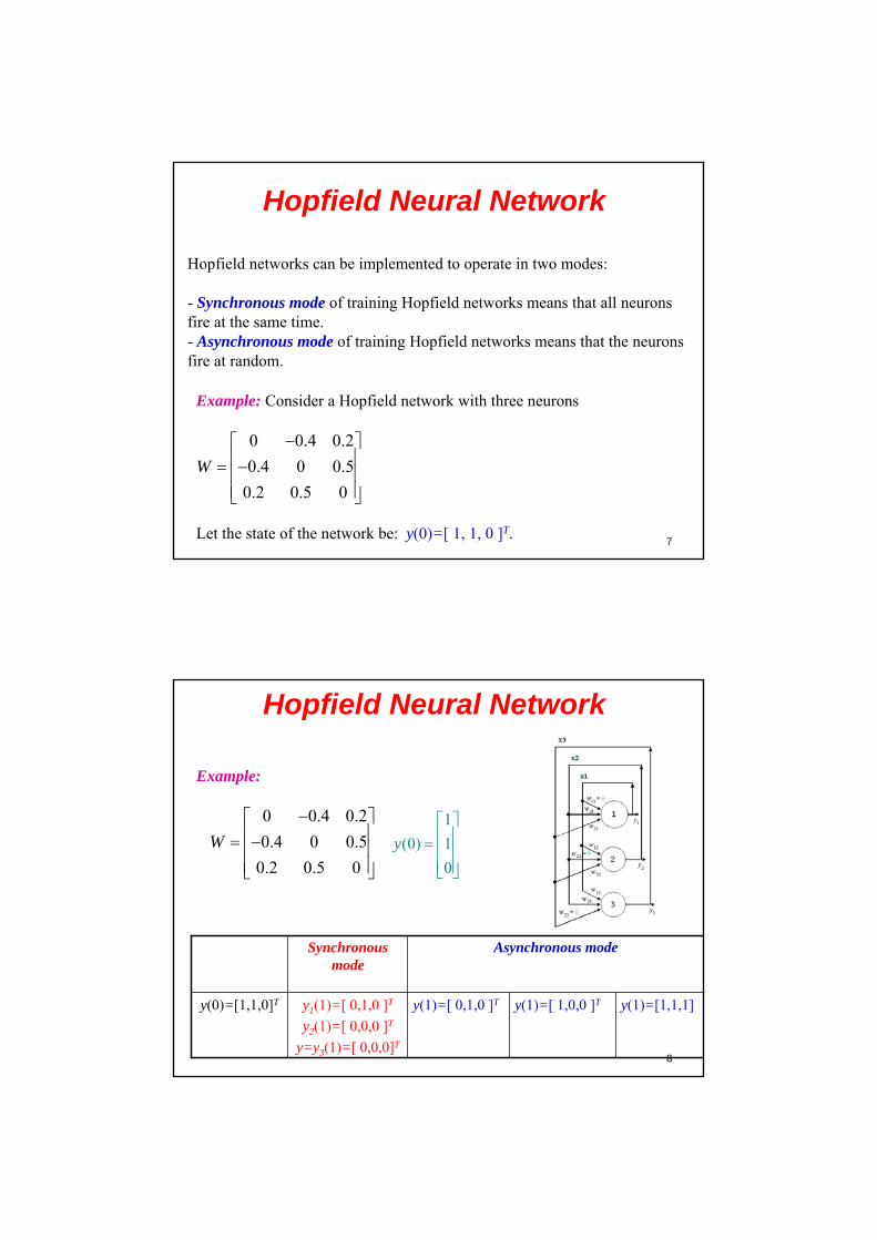
Hopfield networks can be implemented to operate in two modes:
- Synchronous mode of training Hopfield networks means that all neurons fire at the same time.- Asynchronous mode of training Hopfield networks means that the neurons fire at random.
Example: Consider a Hopfield network with three neurons
0 0.4 0.2
0.4 0 0.5
0.2 0.5 0
W
Let the state of the network be: y(0)=[ 1, 1, 0 ]T.
8
Hopfield Neural Network
Example:
0 0.4 0.2
0.4 0 0.5
0.2 0.5 0
W
y(1)=[ 1,0,0 ]Ty(1)=[ 0,1,0 ]T y(1)=[1,1,1]y1(1)=[ 0,1,0 ]T
y2(1)=[ 0,0,0 ]T
y=y3(1)=[ 0,0,0]T
y(0)=[1,1,0]T
Asynchronous modeSynchronous mode
1
(0) 1
0
y
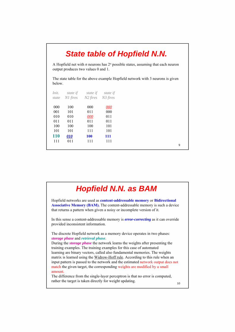
9
State table of Hopfield N.N.A Hopfield net with n neurons has 2n possible states, assuming that each neuron output produces two values 0 and 1.
The state table for the above example Hopfield network with 3 neurons is given below.
Init. state if state if state ifstate N1 fires N2 fires N3 fires
000 100 000 000001 101 011 000010 010 000 011011 011 011 011100 100 100 101101 101 111 101
110 010 100 111111 011 111 111
10
Hopfield N.N. as BAMHopfield networks are used as content-addressable memory or Bidirectional Associative Memory (BAM). The content-addressable memory is such a device that returns a pattern when given a noisy or incomplete version of it.
In this sense a content-addressable memory is error-correcting as it can overrideprovided inconsistent information.
The discrete Hopfield network as a memory device operates in two phases: storage phase and retrieval phase. During the storage phase the network learns the weights after presenting the training examples. The training examples for this case of automatedlearning are binary vectors, called also fundamental memories. The weights matrix is learned using the Widrow-Hoff rule. According to this rule when an input pattern is passed to the network and the estimated network output does not match the given target, the corresponding weights are modified by a small amount. The difference from the single-layer perceptron is that no error is computed, rather the target is taken directly for weight updating.
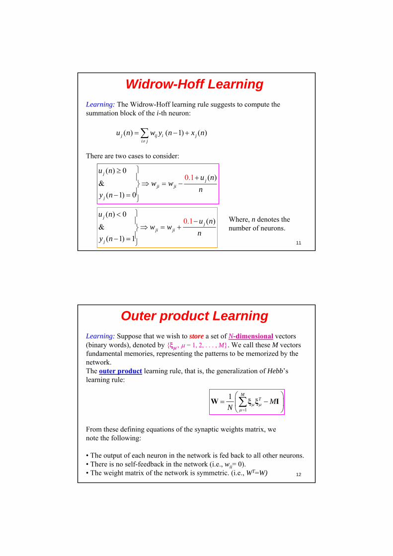
11
Widrow-Hoff LearningLearning: The Widrow-Hoff learning rule suggests to compute the summation block of the i-th neuron:
( ) ( 1) ( )j ij i ji j
u n w y n x n
There are two cases to consider:
( ) 0( )
&
( 1)
0
0
.1j
jji ji
j
u nu n
w wn
y n
( ) 0( )
&
( 1)
0
1
.1j
jji ji
j
u nu n
w wn
y n
Where, n denotes the number of neurons.
12
Outer product LearningLearning: Suppose that we wish to store a set of N-dimensional vectors (binary words), denoted by { = 1, 2, . . . , M}. We call these M vectors fundamental memories, representing the patterns to be memorized by the network.The outer product learning rule, that is, the generalization of Hebb’slearning rule:
1
1 MT M
N
W ξ ξ I
From these defining equations of the synaptic weights matrix, wenote the following:
• The output of each neuron in the network is fed back to all other neurons.• There is no self-feedback in the network (i.e., wii= 0).• The weight matrix of the network is symmetric. (i.e., WT=W)
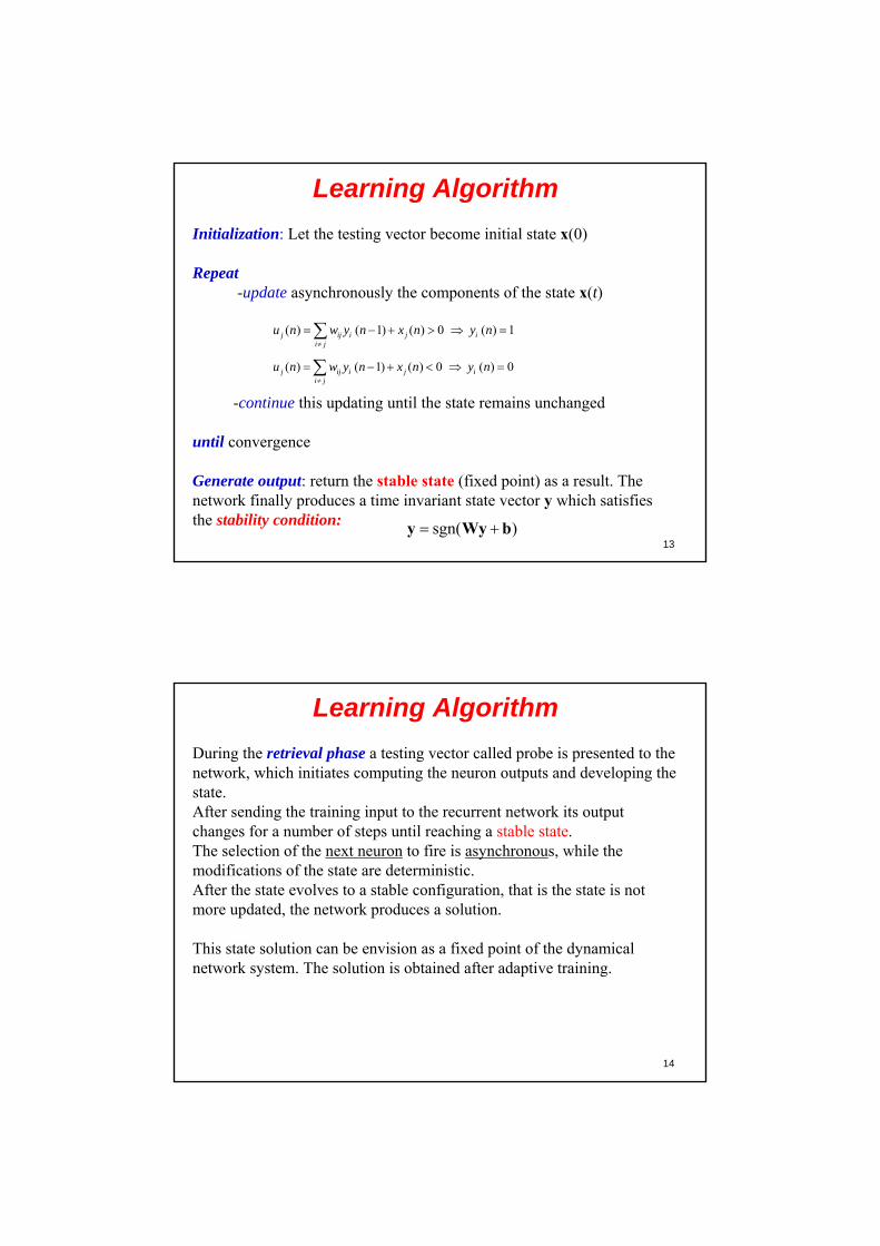
13
Learning Algorithm
Initialization: Let the testing vector become initial state x(0)
Repeat-update asynchronously the components of the state x(t)
-continue this updating until the state remains unchanged
until convergence
Generate output: return the stable state (fixed point) as a result. The network finally produces a time invariant state vector y which satisfies the stability condition:
( ) ( 1) ( ) 0 ( ) 1j ij i j ii j
u n w y n x n y n
sgn( ) y Wy b
( ) ( 1) ( ) 0 ( ) 0j ij i j ii j
u n w y n x n y n
14
Learning Algorithm
During the retrieval phase a testing vector called probe is presented to the network, which initiates computing the neuron outputs and developing the state. After sending the training input to the recurrent network its output changes for a number of steps until reaching a stable state. The selection of the next neuron to fire is asynchronous, while themodifications of the state are deterministic. After the state evolves to a stable configuration, that is the state is not more updated, the network produces a solution.
This state solution can be envision as a fixed point of the dynamical network system. The solution is obtained after adaptive training.
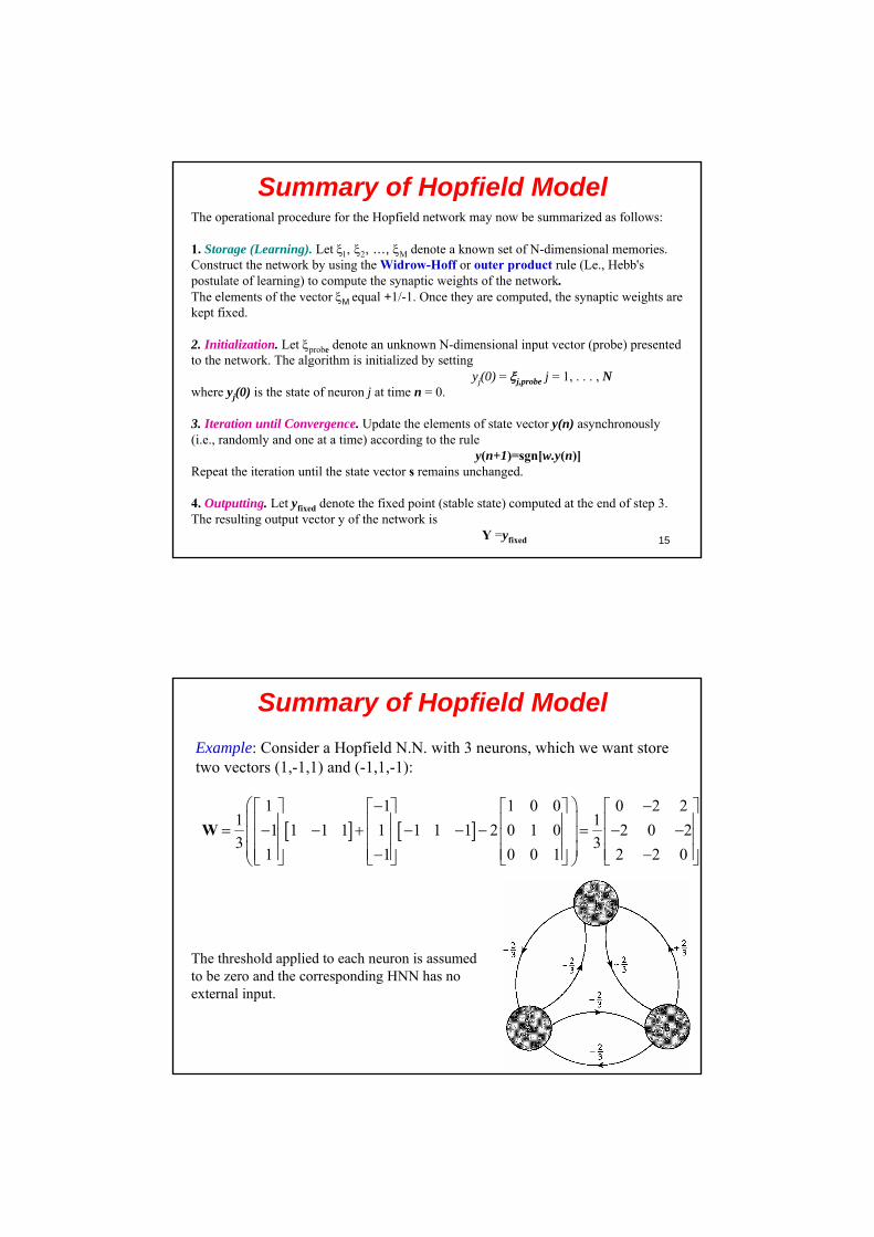
15
Summary of Hopfield ModelThe operational procedure for the Hopfield network may now be summarized as follows:
1. Storage (Learning). Let , …, M denote a known set of N-dimensional memories.Construct the network by using the Widrow-Hoff or outer product rule (Le., Hebb'spostulate of learning) to compute the synaptic weights of the network. The elements of the vector M equal +1/-1. Once they are computed, the synaptic weights are kept fixed.
2. Initialization. Let probe denote an unknown N-dimensional input vector (probe) presentedto the network. The algorithm is initialized by setting
yj(0) = j,probe j = 1, . . . , Nwhere yj(0) is the state of neuron j at time n = 0.
3. Iteration until Convergence. Update the elements of state vector y(n) asynchronously(i.e., randomly and one at a time) according to the rule
y(n+1)=sgn[w.y(n)]Repeat the iteration until the state vector s remains unchanged.
4. Outputting. Let yfixed denote the fixed point (stable state) computed at the end of step 3.The resulting output vector y of the network is
Y =yfixed
16
Summary of Hopfield Model
Example: Consider a Hopfield N.N. with 3 neurons, which we want store two vectors (1,-1,1) and (-1,1,-1):
1 1 1 0 0 0 2 2
1 11 1 1 1 1 1 1 1 2 0 1 0 2 0 2
3 31 1 0 0 1 2 2 0
W
The threshold applied to each neuron is assumed to be zero and the corresponding HNN has no external input.
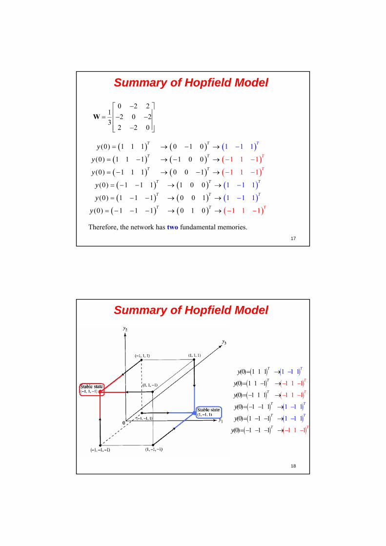
17
Summary of Hopfield Model
Therefore, the network has two fundamental memories.
0 2 21
2 0 23
2 2 0
W
1 1 1
1 1 1
1
(0) 1 1 1 0 1 0
(0) 1 1 1 1 0 0
(0) 1 1 1 0 0 1
(0) 1 1 1 1 0 0
(0) 1 1 1 0 0 1
(0) 1 1 1
1 1
1 1 1
1 1 1
1 1 1 0 1 0
T
T
T
T
T T
T T
T T
T T
T T
T
T
T T
y
y
y
y
y
y
18
Summary of Hopfield Model
(0) 1 1 1
(0) 1 1 1
(0) 1 1 1
(
1 1 1
1 1 1
1
0) 1 1 1
(0) 1 1 1
(0) 1 1 1
1 1
1 1 1
1 1
1 1 1
1
T
T
T
T T
T
T
T
T
T
T
T
y
y
y
y
y
y

19
Literature Cited
The material of this lecture is based on:
[1] Simon Haykin, Neural Networks: A Comprehensive Foundation., Prentice Hall, 1998.
[2] http://homepages.gold.ac.uk/nikolaev/cis311.htm
1
Genetic Algorithm
Lecture 15
Introduction to G.A.
2
Optimization
In mathematics and engineering science, optimization, refers to choosing the best element from some set of available alternatives.
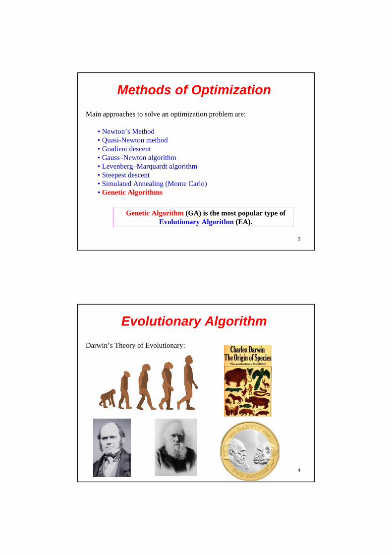
3
Methods of Optimization
Main approaches to solve an optimization problem are:
• Newton’s Method• Quasi-Newton method • Gradient descent • Gauss–Newton algorithm • Levenberg–Marquardt algorithm• Steepest descent• Simulated Annealing (Monte Carlo)• Genetic Algorithms
Genetic Algorithm (GA) is the most popular type of Evolutionary Algorithm (EA).
4
Evolutionary Algorithm
Darwin’s Theory of Evolutionary:
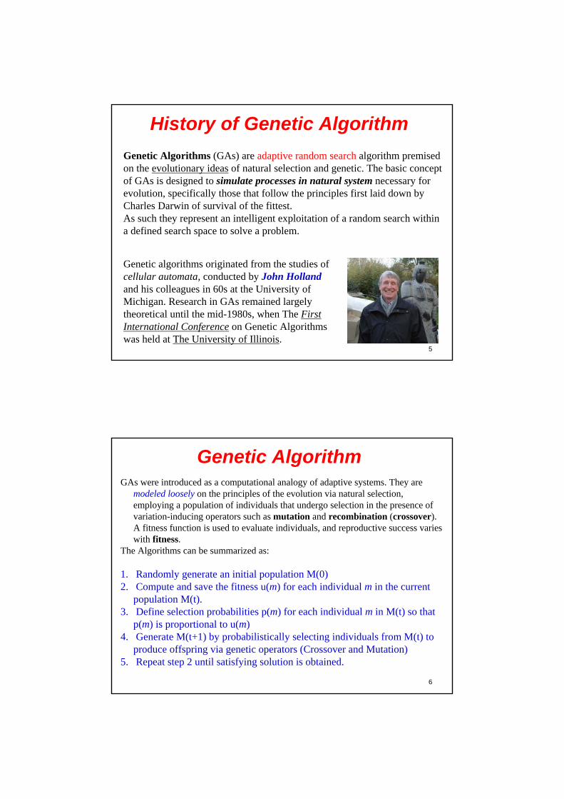
5
History of Genetic Algorithm
Genetic Algorithms (GAs) are adaptive random search algorithm premised on the evolutionary ideas of natural selection and genetic. The basic concept of GAs is designed to simulate processes in natural system necessary for evolution, specifically those that follow the principles first laid down by Charles Darwin of survival of the fittest. As such they represent an intelligent exploitation of a random search within a defined search space to solve a problem.
Genetic algorithms originated from the studies of cellular automata, conducted by John Hollandand his colleagues in 60s at the University of Michigan. Research in GAs remained largely theoretical until the mid-1980s, when The First International Conference on Genetic Algorithms was held at The University of Illinois.
6
Genetic AlgorithmGAs were introduced as a computational analogy of adaptive systems. They are
modeled loosely on the principles of the evolution via natural selection, employing a population of individuals that undergo selection in the presence of variation-inducing operators such as mutation and recombination (crossover). A fitness function is used to evaluate individuals, and reproductive success varies with fitness.
The Algorithms can be summarized as:
1. Randomly generate an initial population M(0) 2. Compute and save the fitness u(m) for each individual m in the current
population M(t). 3. Define selection probabilities p(m) for each individual m in M(t) so that
p(m) is proportional to u(m) 4. Generate M(t+1) by probabilistically selecting individuals from M(t) to
produce offspring via genetic operators (Crossover and Mutation)5. Repeat step 2 until satisfying solution is obtained.
7
GA and Biological background
1. Randomly generate an initial population
• Genetic information is stored in the chromosomes.• Each chromosome is build of DNA• Chromosomes in humans form pairs• The chromosome is divided in parts: genes• Genes code for properties
8
GA and Biological background2. Compute and save the fitness u(m) for each individual m in the current
population M(t).
3. Define selection probabilities p(m) for each individual m in M(t) so that p(m) is proportional to u(m)
4. Generate M(t+1) by probabilistically selecting individuals from M(t) to produce offspring via genetic operators (Crossover and Mutation)
offspring
9
Genetic Algorithm
GAs are useful and efficient when
• The search space is large, complex or poorly understood. • Domain knowledge is scarce or expert knowledge is difficult to
encode to narrow the search space.• No mathematical analysis is available. • Traditional search methods fail.
10
Genetic Algorithm
0 START : Create random population of n chromosomes
1 FITNESS : Evaluate fitness f(x) of each chromosome in the population
2 NEW POPULATION (using Genetic operations)0 SELECTION : Based on f(x)1 RECOMBINATION : Cross-over chromosomes2 MUTATION : Mutate chromosomes3 ACCEPTATION : Reject or accept new one
3 REPLACE : Replace old with new population: the new generation
4 TEST : Test problem criterium
5 LOOP : Continue step 1 – 4 until criterium is satisfied
Basic algorithm of Genetic algorithm
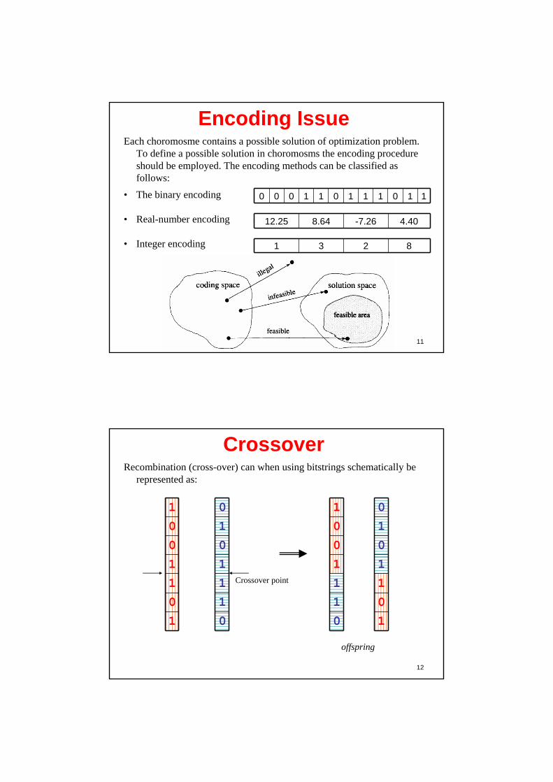
11
Encoding IssueEach choromosme contains a possible solution of optimization problem.
To define a possible solution in choromosms the encoding procedure should be employed. The encoding methods can be classified as follows:
• The binary encoding
• Real-number encoding
• Integer encoding
0 0 0 1 1 0 1 1 1 0 1 1
12.25 8.64 -7.26 4.40
1 3 2 8
12
CrossoverRecombination (cross-over) can when using bitstrings schematically be
represented as:
1
0
0
1
1
0
1
0
1
0
1
1
1
0
1
0
0
1
1
1
0
0
1
0
1
1
0
1
Crossover point
offspring
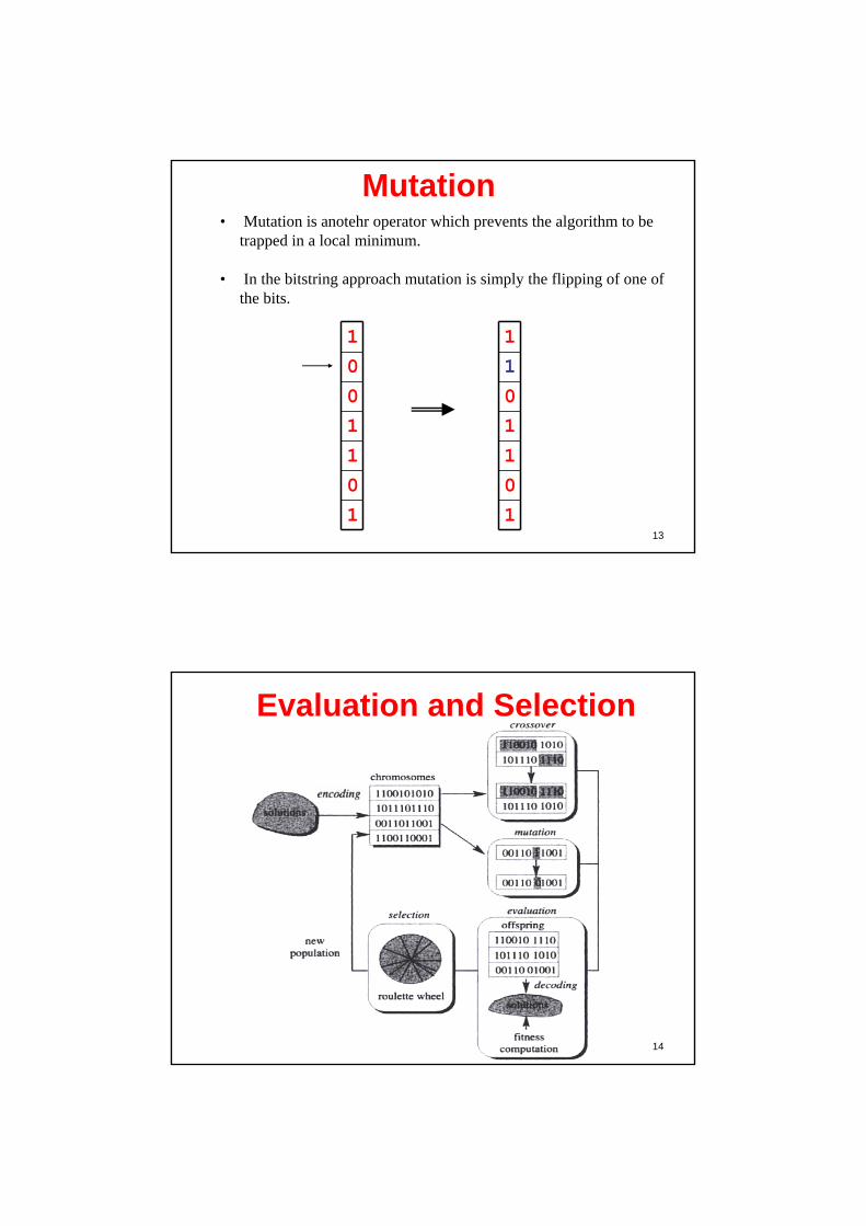
13
Mutation• Mutation is anotehr operator which prevents the algorithm to be
trapped in a local minimum.
• In the bitstring approach mutation is simply the flipping of one of the bits.
1
0
0
1
1
0
1
1
1
0
1
1
0
1
14
Evaluation and Selection
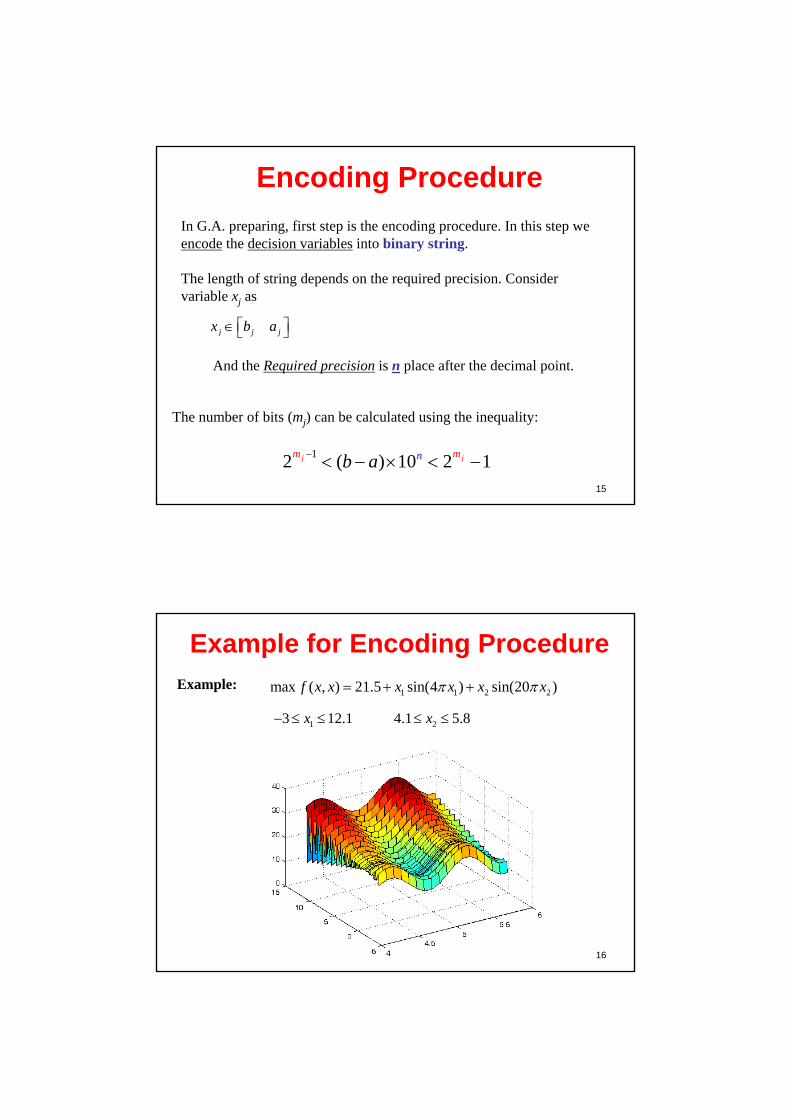
15
Encoding Procedure
In G.A. preparing, first step is the encoding procedure. In this step we encode the decision variables into binary string.
The length of string depends on the required precision. Considervariable xj as
j j jx b a
And the Required precision is n place after the decimal point.
12 ( ) 10 2 1j jm n mb a
The number of bits (mj) can be calculated using the inequality:
16
Example for Encoding ProcedureExample:
13 12.1x
1 1 2 2max ( , ) 21.5 sin(4 ) sin(20 )f x x x x x x
24.1 5.8x
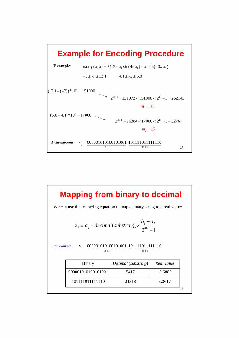
17
Example for Encoding ProcedureExample:
13 12.1x
1 1 2 2max ( , ) 21.5 sin(4 ) sin(20 )f x x x x x x
24.1 5.8x
4(12.1 ( 3))*10 151000 18 1 182 131072 151000 2 1 262143
4(5.8 4.1)*10 17000 15 1 152 16384 17000 2 1 32767
1 18m
2 15m
18 bit 15 bit
000001010100101001 101111011111110jv A chromosome:
18
Mapping from binary to decimalWe can use the following equation to map a binary string to a real value:
18 bit 15 bit
000001010100101001 101111011111110jv For example:
( )2 1j
j jj j m
b ax a decimal substring
Binary Decimal (substring) Real value
000001010100101001 5417 -2.6880
101111011111110 24318 5.3617
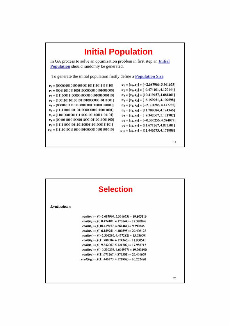
19
Initial PopulationIn GA process to solve an optimization problem in first step an Initial Population should randomly be generated.
To generate the initial population firstly define a Population Size.
20
Selection
Evaluation:
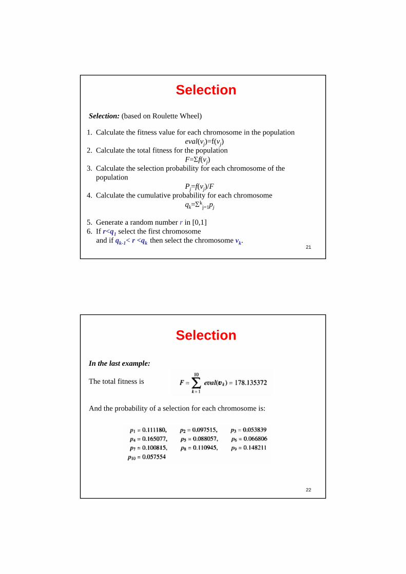
21
Selection
Selection: (based on Roulette Wheel)
1. Calculate the fitness value for each chromosome in the populationeval(vj)=f(vj)
2. Calculate the total fitness for the populationF=f(vj)
3. Calculate the selection probability for each chromosome of the population
Pj=f(vj)/F4. Calculate the cumulative probability for each chromosome
qk=kj=1pj
5. Generate a random number r in [0,1]6. If r<q1 select the first chromosome
and if qk-1< r <qk then select the chromosome vk.
22
Selection
In the last example:
The total fitness is
And the probability of a selection for each chromosome is:
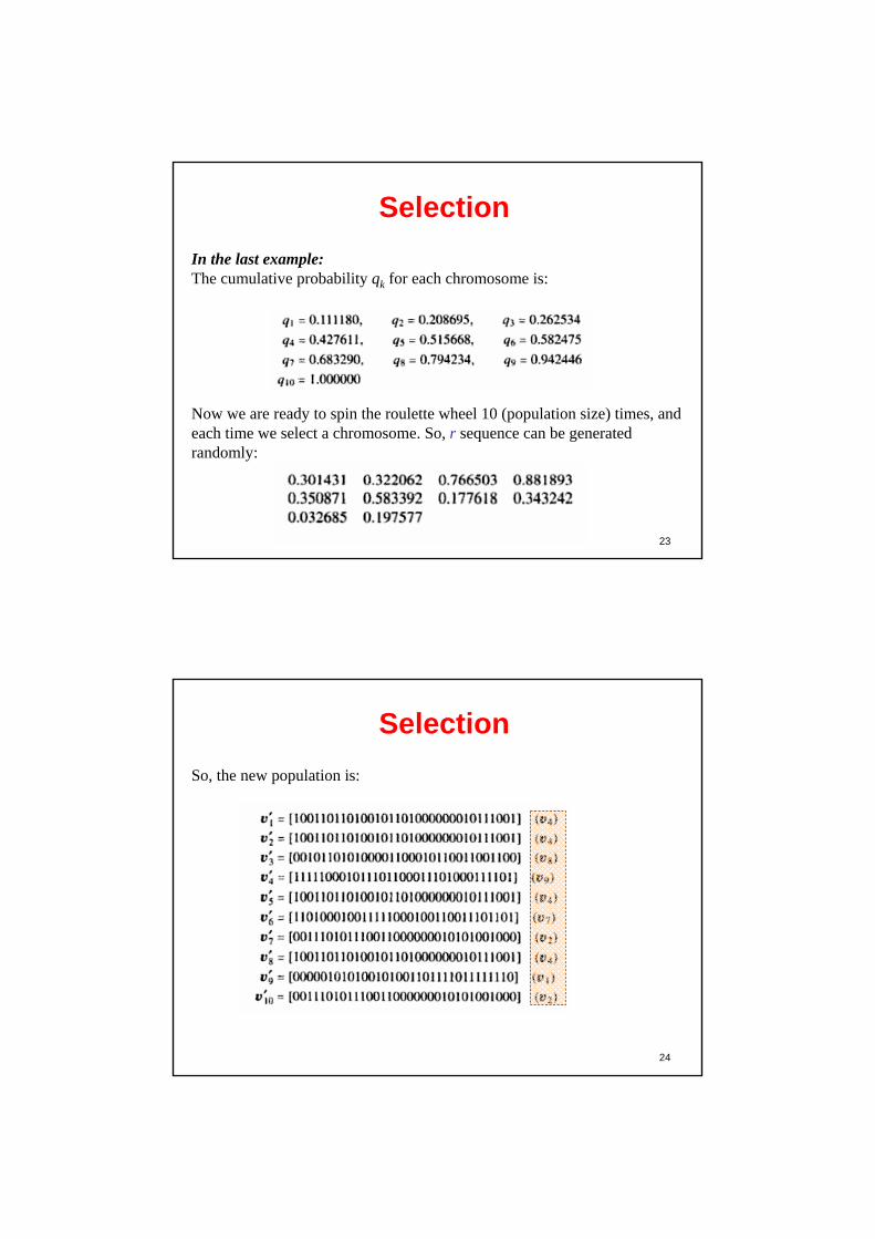
23
Selection
In the last example:The cumulative probability qk for each chromosome is:
Now we are ready to spin the roulette wheel 10 (population size) times, and each time we select a chromosome. So, r sequence can be generated randomly:
24
Selection
So, the new population is:
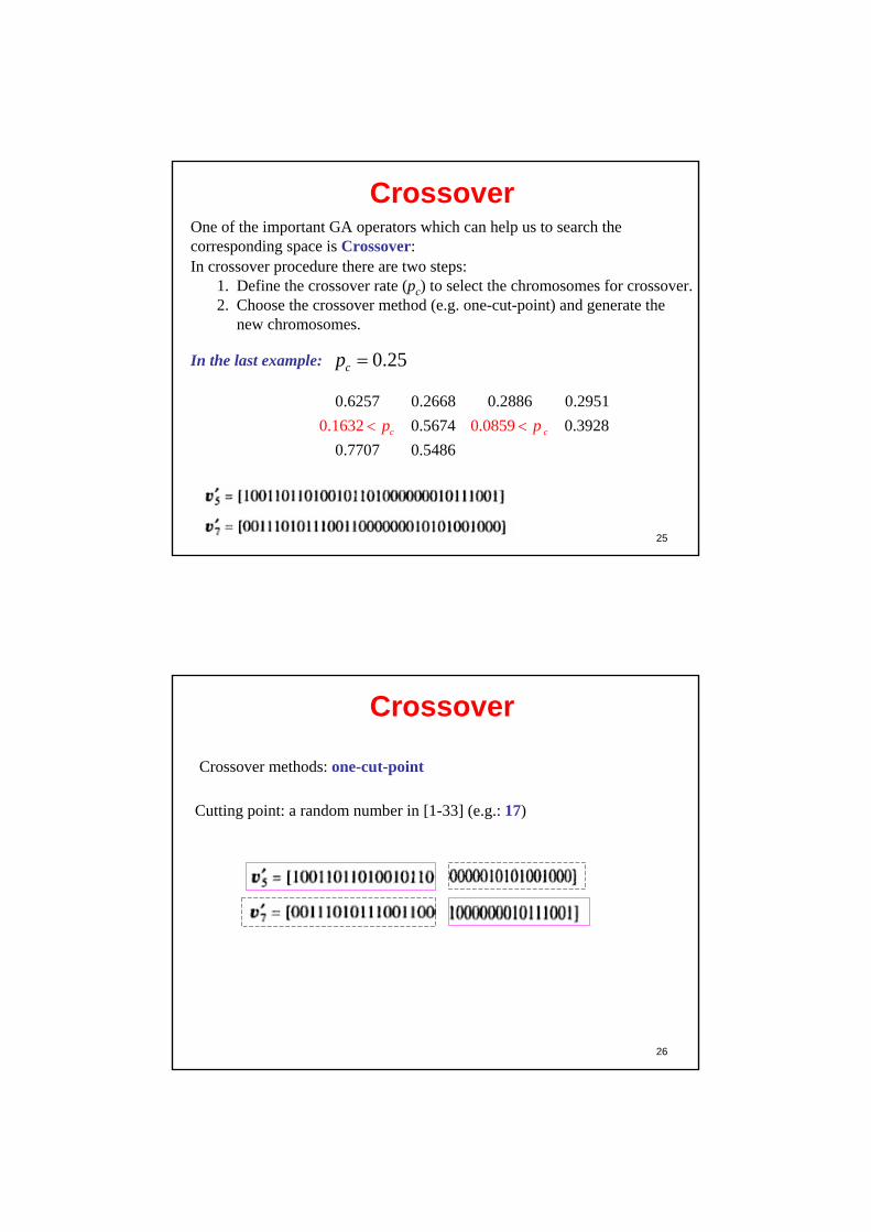
25
CrossoverOne of the important GA operators which can help us to search the corresponding space is Crossover:In crossover procedure there are two steps:
1. Define the crossover rate (pc) to select the chromosomes for crossover.2. Choose the crossover method (e.g. one-cut-point) and generate the
new chromosomes.
In the last example: 0.25cp
0.6257 0.2668 0.2886 0.2951
00. .5674 0.3928
0.7707 0.5486
1632 0.0859c cp p
26
Crossover
Crossover methods: one-cut-point
Cutting point: a random number in [1-33] (e.g.: 17)
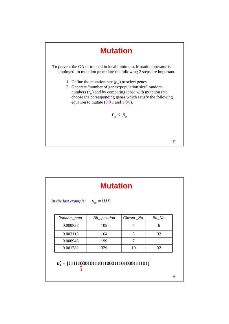
27
Mutation
To prevent the GA of trapped in local minimum, Mutation operator is employed. In mutation procedure the following 2 steps are important.
1. Define the mutation rate (pm) to select genes.2. Generate “number of genes*population size” random
numbers (rm) and by comparing those with mutation rate choose the corresponding genes which satisfy the following equation to mutate (01 and 10).
m mr p
28
Mutation
In the last example: 0.01mp
Random_num. Bit_ position Chrom._No. Bit_No.
0.009857 105 4 6
0.003113 164 5 32
0.000946 199 7 1
0.001282 329 10 32
1
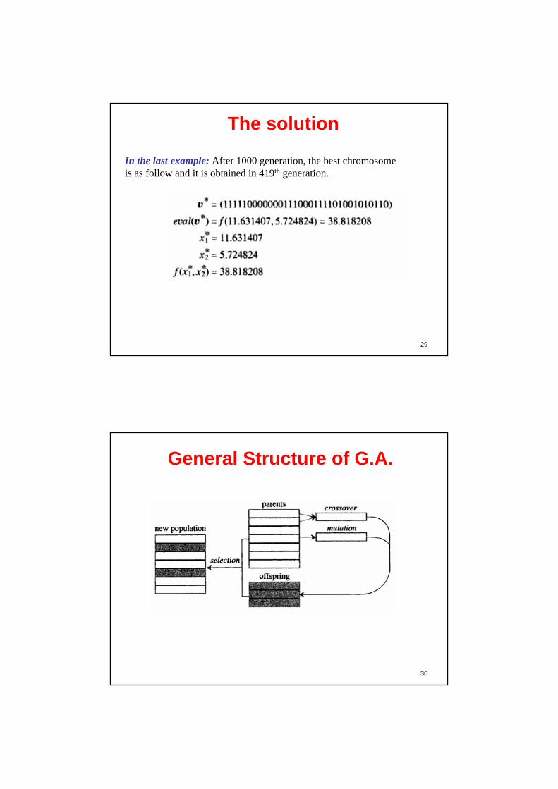
29
The solution
In the last example: After 1000 generation, the best chromosome is as follow and it is obtained in 419th generation.
30
General Structure of G.A.
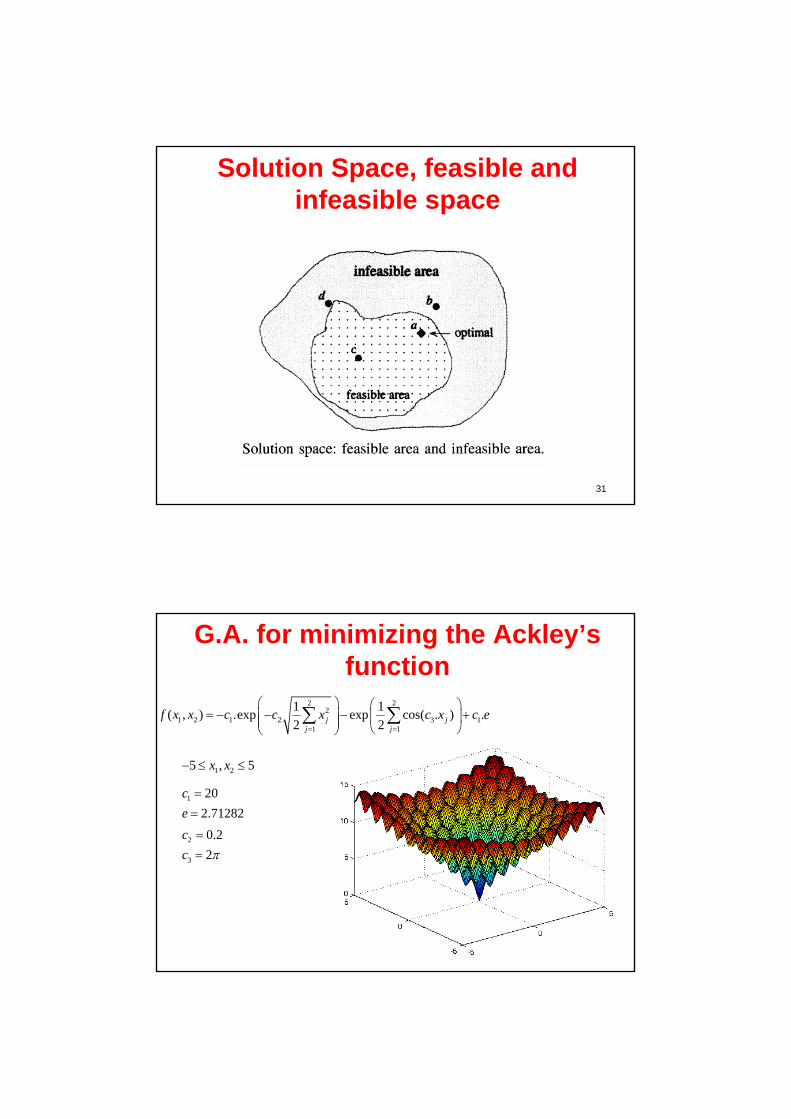
31
Solution Space, feasible and infeasible space
32
G.A. for minimizing the Ackley’s function
2 22
1 2 1 2 3 11 1
1 1( , ) .exp exp cos( . ) .
2 2j jj j
f x x c c x c x c e
1 25 , 5x x
1
2
3
20
2.71282
0.2
2
c
e
c
c
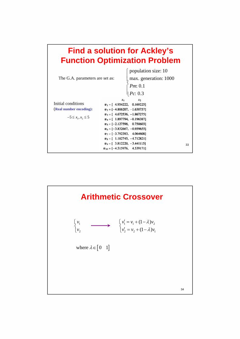
33
Find a solution for Ackley’s Function Optimization Problem
population size: 10
max. generation: 1000
: 0.1
: 0.3
Pm
Pc
The G.A. parameters are set as:
Initial conditions(Real number encoding):
1 25 , 5x x
34
Arithmetic Crossover
1 1 2
2 2 1
(1 )
(1 )
v v v
v v v
1
2
v
v
where 0 1
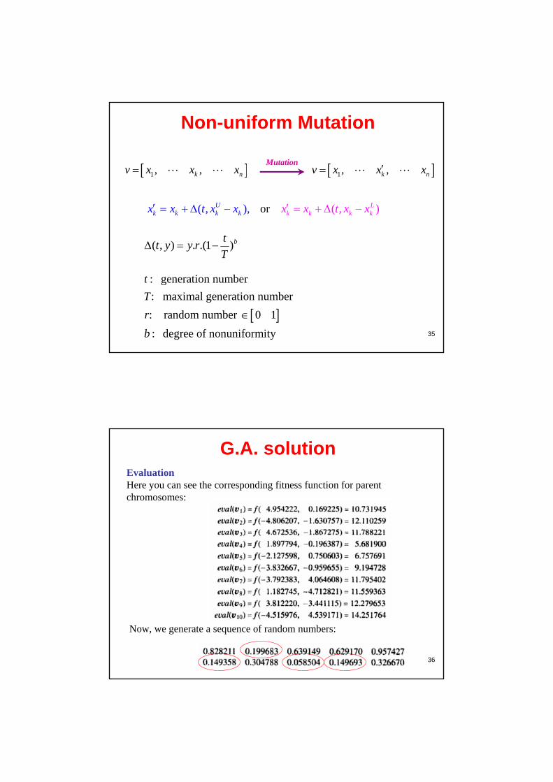
35
Non-uniform Mutation
1, ,k nv x x x 1, ,k nv x x x Mutation
or ( , ), ( , )Uk k k k
Lk k k kx x xx t x x t x x
( , ) . .(1 )btt y y r
T
: generation number
: maximal generation number
: random number 0 1
: degree of nonuniformity
t
T
r
b
36
G.A. solutionEvaluationHere you can see the corresponding fitness function for parent chromosomes:
Now, we generate a sequence of random numbers:
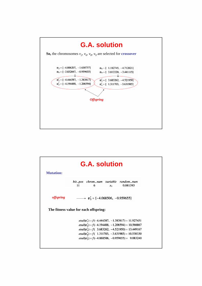
G.A. solutionSo, the chromosomes v2, v6, v8, v9 are selected for crossover
Offspring
G.A. solutionMutation:
offspring
The fitness value for each offspring:

39
7th Mini Project
In this project, by using of G.A. you should find the minimum point of Ackley’s function.
40
Literature Cited
The material of this lecture is based on:
[1] Mitsuo Gen, Runwei Cheng, Genetic Algorithms and Engineering Design., Wiley-Interscience, 1997.