Chapter 5: JOINT PROBABILITYDISTRIBUTIONS

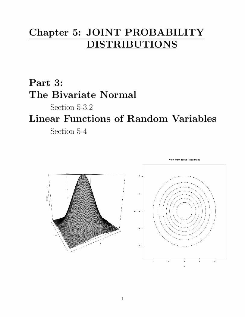
Part 3:The Bivariate Normal

Section 5-3.2

Linear Functions of Random VariablesSection 5-4

1

The bivariate normal is kind of nifty because...

• The marginal distributions of X and Y areboth univariate normal distributions.

• The conditional distribution of Y given X isa normal distribution.

• The conditional distribution of X given Y isa normal distribution.

• Linear combinations of X and Y (such asZ = 2X + 4Y ) follow a normal distribution.

• It’s normal almost any way you slice it.

2

•Bivariate Normal ProbabilityDensity Function

The parameters: µX , µY , σX , σY , ρ

fXY (x, y) =1

2πσXσY√

(1− ρ2)×

exp

{−1

2(1− ρ2)

[(x− µX)2

σ2X

− 2ρ(x− µX)(y − µY )

σXσY+

(y − µY )2

σ2Y

]}

for −∞ < x <∞ and −∞ < y <∞, with

parameters σX > 0 , σY > 0 ,−∞ < µX <∞, −∞ < µY <∞,

and −1 < ρ < 1.

Where ρ is the correlation between X and Y .

The other parameters are the needed parame-ters for the marginal distributions of X and Y .

3

•Bivariate Normal

When X and Y are independent, the con-tour plot of the joint distribution looks like con-centric circles (or ellipses, if they have differentvariances) with major/minor axes that are par-allel/perpendicular to the x-axis:

The center of each circle or ellipse is at (µX , µY ).

4

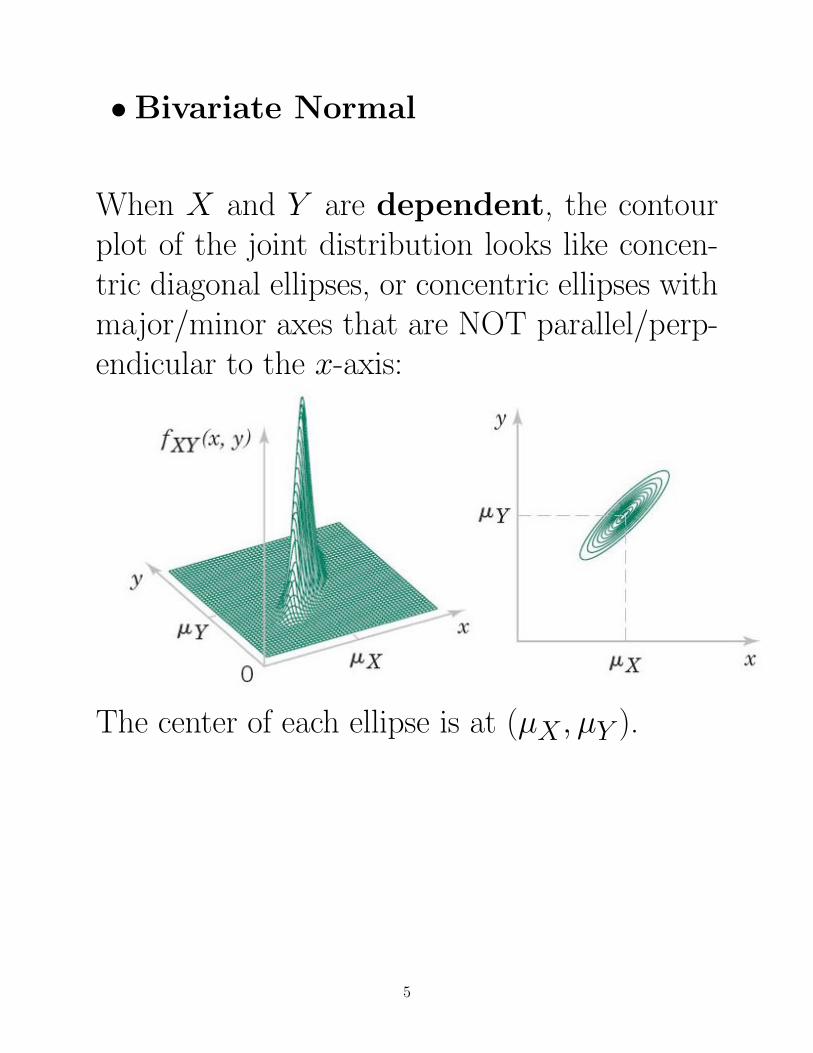
•Bivariate Normal

When X and Y are dependent, the contourplot of the joint distribution looks like concen-tric diagonal ellipses, or concentric ellipses withmajor/minor axes that are NOT parallel/perp-endicular to the x-axis:

The center of each ellipse is at (µX , µY ).

5

•Marginal distributions of X and Y inthe Bivariate Normal

Marginal distributions of X and Y are nor-mal:

X ∼ N(µX , σ2X) and Y ∼ N(µY , σ

2Y )

Know how to take the parameters from thebivariate normal and calculate probabilitiesin a univariate X or Y problem.

•Conditional distribution of Y |x in theBivariate Normal

The conditional distribution of Y |x is alsonormal:

Y |x ∼ N(µY |x, σ2Y |x)

6

Y |x ∼ N(µY |x, σ2Y |x)

where the “mean of Y |x” or µY |x dependson the given x-value as

µY |x = µY + ρσYσX

(x− µX)

and “variance of Y |x” or σ2Y |x depends on

the correlation as

σ2Y |x = σ2

Y (1− ρ2).

Know how to take the parameters from thebivariate normal and get a conditional distri-bution for a given x-value, and then calculateprobabilities for the conditional distributionof Y |x (which is a univariate distribution).

Remember that probabilities in the normalcase will be found using the z-table.

7

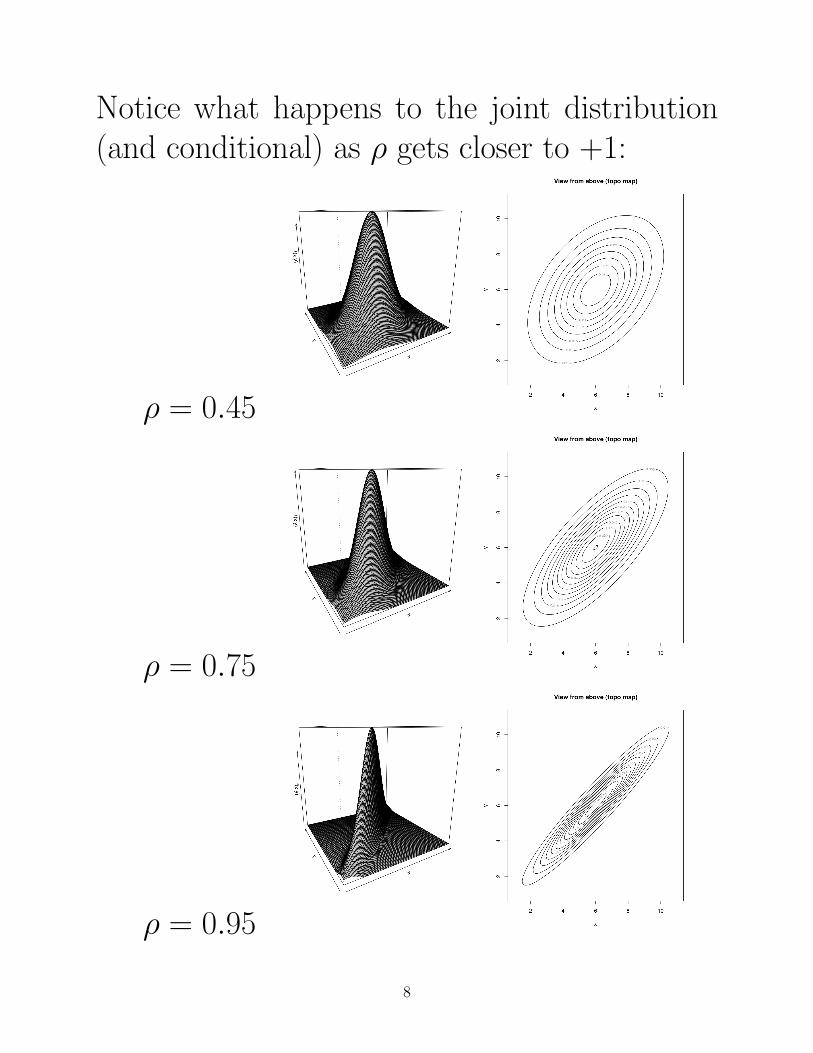
Notice what happens to the joint distribution(and conditional) as ρ gets closer to +1:

ρ = 0.45

ρ = 0.75

ρ = 0.95

8

As a last note on the bivariate normal...

Though ρ = 0 does not mean X and Y are in-dependent in all cases, for the bivariate normal,this does hold.

For the Bivariate Normal,Zero Correlation Implies Independence

If X and Y have a bivariate normal distribution(so, we know the shape of the joint distribution),then with ρ = 0, we have X and Y as indepen-dent.

9

• Example: From book problem 5-54.

Assume X and Y have a bivariate normaldistribution with..µX = 120, σX = 5µY = 100, σY = 2ρ = 0.6

Determine:(i) Marginal probability distribution of X .

(ii) Conditional probability distribution of Ygiven that X = 125.

10

Linear Functions of Random VariablesSection 5-4

• Linear Combination

Given random variables X1, X2, . . . , Xp andconstants c1, c2, . . . , cp,

Y = c1X1 + c2X2 + · · · + cpXp

is a linear combination of X1, X2, . . . , Xp.

•Mean of a Linear Function

If Y = c1X1 + c2X2 + · · · + cpXp,

E(Y ) = c1E(X1)+c2E(X2)+· · ·+cpE(Xp)

11

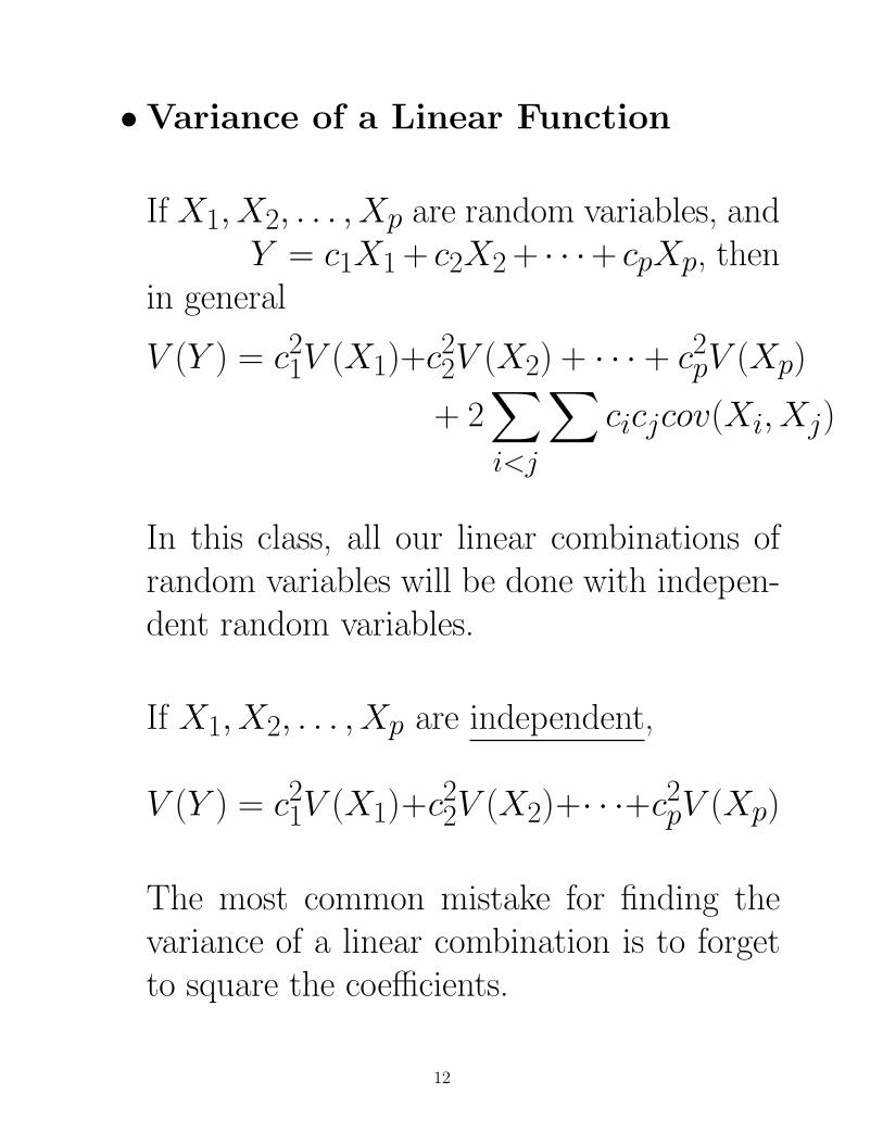
•Variance of a Linear Function

If X1, X2, . . . , Xp are random variables, andY = c1X1 + c2X2 + · · ·+ cpXp, then

in general

V (Y ) = c21V (X1)+c2

2V (X2) + · · · + c2pV (Xp)

+ 2∑i<j

∑cicjcov(Xi, Xj)

In this class, all our linear combinations ofrandom variables will be done with indepen-dent random variables.

If X1, X2, . . . , Xp are independent,

V (Y ) = c21V (X1)+c2

2V (X2)+· · ·+c2pV (Xp)

The most common mistake for finding thevariance of a linear combination is to forgetto square the coefficients.

12

• Example: Semiconductor product (exam-ple 5-31)

A semiconductor product consists of threelayers. The variance of the thickness of thefirst, second, third layers are 25, 40, and 30nanometers2.

What is the variance of the thickness of thefinal product?

ANS:

13

•Mean and Variance of an Average

If X̄ =(X1+X2+···+Xp)

p

with E(Xi) = µ for i = 1, 2, . . . , p then

E(X̄) = µ.

The expected value of the average of p ran-dom variables, all with the same mean µ,is just µ again.

If X1, X2, . . . , Xp are also independent with

V (Xi) = σ2 for i = 1, 2, . . . , p then

V (X̄) =σ2

p

The variance of the average of p randomvariables is smaller than the variance of asingle random variable.

14

•Reproductive Property of theNormal Distribution

If X1, X2, . . . , Xp are independent, normalrandom variables with E(Xi) = µi andV (Xi) = σ2

i for i = 1, 2, . . . , p,

Y = c1X1 + c2X2 + · · · + cpXp

is a normal random variable with

µY = E(Y ) = c1µ1 + c2µ2 + · · · + cpµp

and

σ2Y = V (Y ) = c2

1σ21 + c2

2σ22 + · · · + c2

pσ2p

i.e. Y ∼ N(µY , σ2Y ) as described above.

A linear combination of normal r.v.’s is also normal.

15

• Example: Weights of people

Assume that the weights of individuals areindependent and normally distributed witha mean of 160 pounds and a standard devi-ation of 30 pounds. Suppose that 25 peoplesqueeze into an elevator that is designed tohold 4300 pounds.

a) What is the probability that the load ex-ceeds the design limit?

16

17