Applied Statistics and Probability for Engineersie230.cankaya.edu.tr/uploads/files/ch05.pdf · 1....
63
Copyright © 2014 John Wiley & Sons, Inc. All rights reserved. Copyright © 2014 John Wiley & Sons, Inc. All rights reserved. Chapter 5 Joint Probability Distributions Applied Statistics and Probability for Engineers Sixth Edition Douglas C. Montgomery George C. Runger
Transcript of Applied Statistics and Probability for Engineersie230.cankaya.edu.tr/uploads/files/ch05.pdf · 1....
Copyright © 2014 John Wiley & Sons, Inc. All rights reserved.Copyright © 2014 John Wiley & Sons, Inc. All rights reserved.
Chapter 5Joint Probability Distributions
Applied Statistics and Probability for
Engineers
Sixth Edition
Douglas C. Montgomery George C. Runger
Copyright © 2014 John Wiley & Sons, Inc. All rights reserved.
Chapter 5 Title and Outline2
5Joint Probability
Distributions
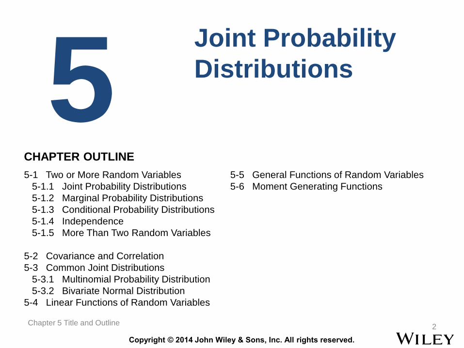
5-1 Two or More Random Variables
5-1.1 Joint Probability Distributions
5-1.2 Marginal Probability Distributions
5-1.3 Conditional Probability Distributions
5-1.4 Independence
5-1.5 More Than Two Random Variables
5-2 Covariance and Correlation
5-3 Common Joint Distributions
5-3.1 Multinomial Probability Distribution
5-3.2 Bivariate Normal Distribution
5-4 Linear Functions of Random Variables
5-5 General Functions of Random Variables
5-6 Moment Generating Functions
CHAPTER OUTLINE
Copyright © 2014 John Wiley & Sons, Inc. All rights reserved.
Learning Objectives for Chapter 5
After careful study of this chapter, you should be able to do the
following:1. Use joint probability mass functions and joint probability density
functions to calculate probabilities.
2. Calculate marginal and conditional probability distributions from joint probability distributions.
3. Interpret and calculate covariances and correlations between random variables.
4. Use the multinomial distribution to determine probabilities.
5. Properties of a bivariate normal distribution and to draw contour plots for the probability density function.
6. Calculate means and variances for linear combinations of random variables, and calculate probabilities for linear combinations of normally distributed random variables.
7. Determine the distribution of a general function of a random variable.
8. Calculate moment generating functions and use them to determine moments and distributions
3Chapter 5 Learning Objectives
Copyright © 2014 John Wiley & Sons, Inc. All rights reserved.
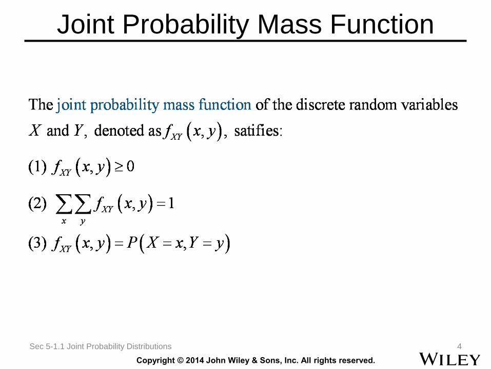
Joint Probability Mass Function
Sec 5-1.1 Joint Probability Distributions 4
Copyright © 2014 John Wiley & Sons, Inc. All rights reserved.
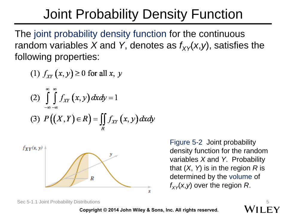
Joint Probability Density Function
Sec 5-1.1 Joint Probability Distributions 5
Figure 5-2 Joint probability
density function for the random
variables X and Y. Probability
that (X, Y) is in the region R is
determined by the volume of
fXY(x,y) over the region R.
The joint probability density function for the continuous
random variables X and Y, denotes as fXY(x,y), satisfies the
following properties:
Copyright © 2014 John Wiley & Sons, Inc. All rights reserved.
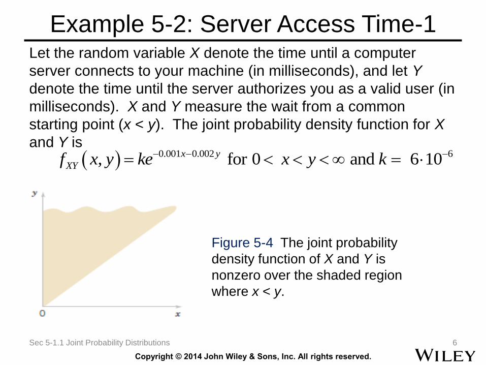
Example 5-2: Server Access Time-1Let the random variable X denote the time until a computer
server connects to your machine (in milliseconds), and let Y
denote the time until the server authorizes you as a valid user (in
milliseconds). X and Y measure the wait from a common
starting point (x < y). The joint probability density function for X
and Y is
Sec 5-1.1 Joint Probability Distributions 6
Figure 5-4 The joint probability
density function of X and Y is
nonzero over the shaded region
where x < y.
0.001 0.002 6, for 0 and 6 10x y
XYf x y ke x y k
Copyright © 2014 John Wiley & Sons, Inc. All rights reserved.
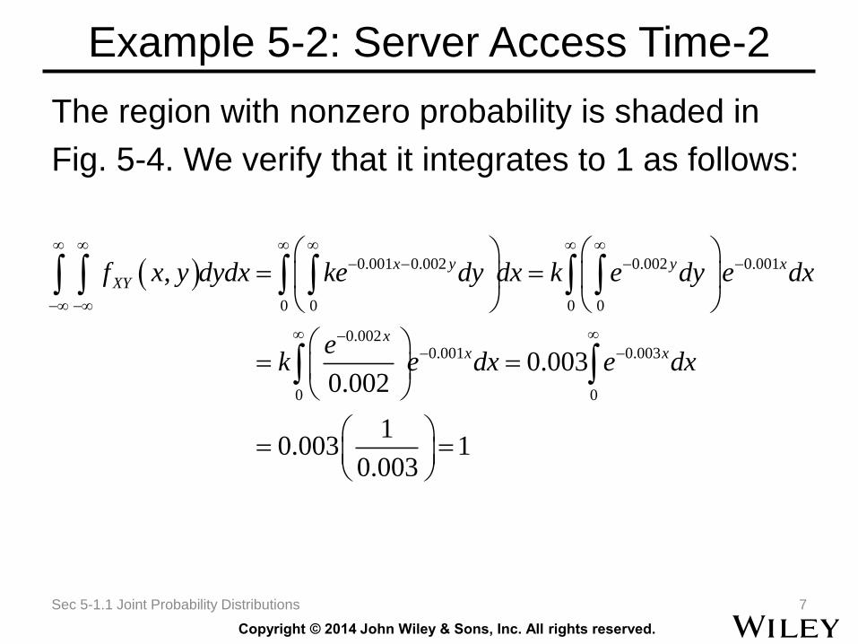
Example 5-2: Server Access Time-2
The region with nonzero probability is shaded in
Fig. 5-4. We verify that it integrates to 1 as follows:
Sec 5-1.1 Joint Probability Distributions 7
0.001 0.002 0.002 0.001
0 0 0 0
0.0020.001 0.003
0 0
,
0.0030.002
10.003 1
0.003
x y y x
XY
xx x
f x y dydx ke dy dx k e dy e dx
ek e dx e dx
Copyright © 2014 John Wiley & Sons, Inc. All rights reserved.
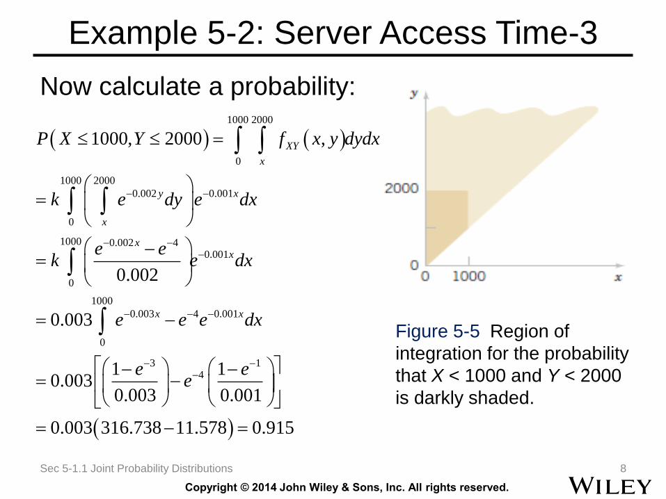
Example 5-2: Server Access Time-3
Now calculate a probability:
Sec 5-1.1 Joint Probability Distributions 8
Figure 5-5 Region of
integration for the probability
that X < 1000 and Y < 2000
is darkly shaded.
1000 2000
0
1000 2000
0.002 0.001
0
1000 0.002 40.001
0
1000
0.003 4 0.001
0
3 14
1000, 2000 ,
0.002
0.003
1 10.003
0.003 0.001
XY
x
y x
x
xx
x x
P X Y f x y dydx
k e dy e dx
e ek e dx
e e e dx
e ee
0.003 316.738 11.578 0.915
Copyright © 2014 John Wiley & Sons, Inc. All rights reserved.
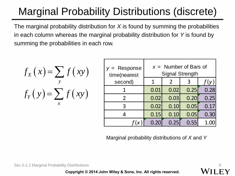
Marginal Probability Distributions (discrete)
The marginal probability distribution for X is found by summing the probabilities
in each column whereas the marginal probability distribution for Y is found by
summing the probabilities in each row.
Sec 5-1.2 Marginal Probability Distributions 9
X
y
Y
x
f x f xy
f y f xy
1 2 3 f (y )
1 0.01 0.02 0.25 0.28
2 0.02 0.03 0.20 0.25
3 0.02 0.10 0.05 0.17
4 0.15 0.10 0.05 0.30
f (x ) 0.20 0.25 0.55 1.00
y = Response
time(nearest
second)
x = Number of Bars of
Signal Strength
Marginal probability distributions of X and Y
Copyright © 2014 John Wiley & Sons, Inc. All rights reserved.
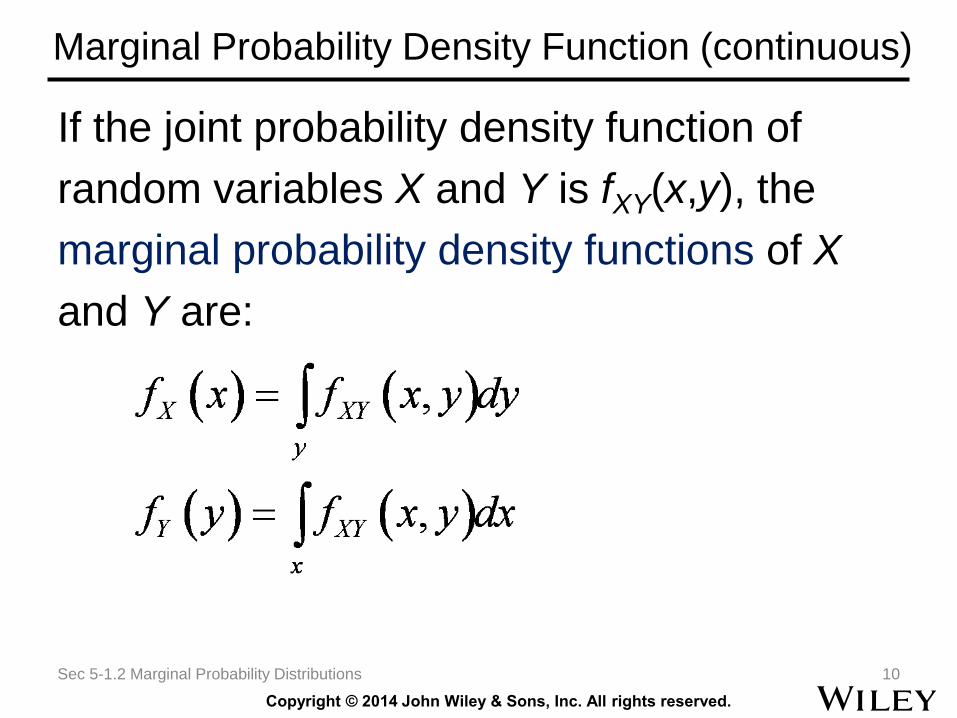
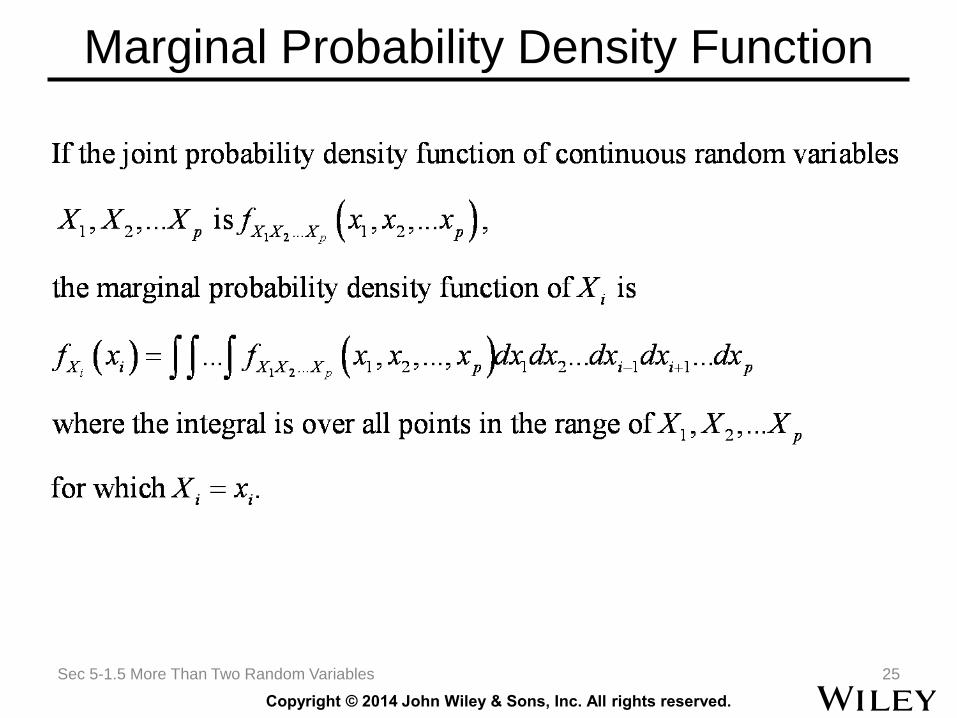
Marginal Probability Density Function (continuous)
If the joint probability density function of
random variables X and Y is fXY(x,y), the
marginal probability density functions of X
and Y are:
Sec 5-1.2 Marginal Probability Distributions 10
Copyright © 2014 John Wiley & Sons, Inc. All rights reserved.
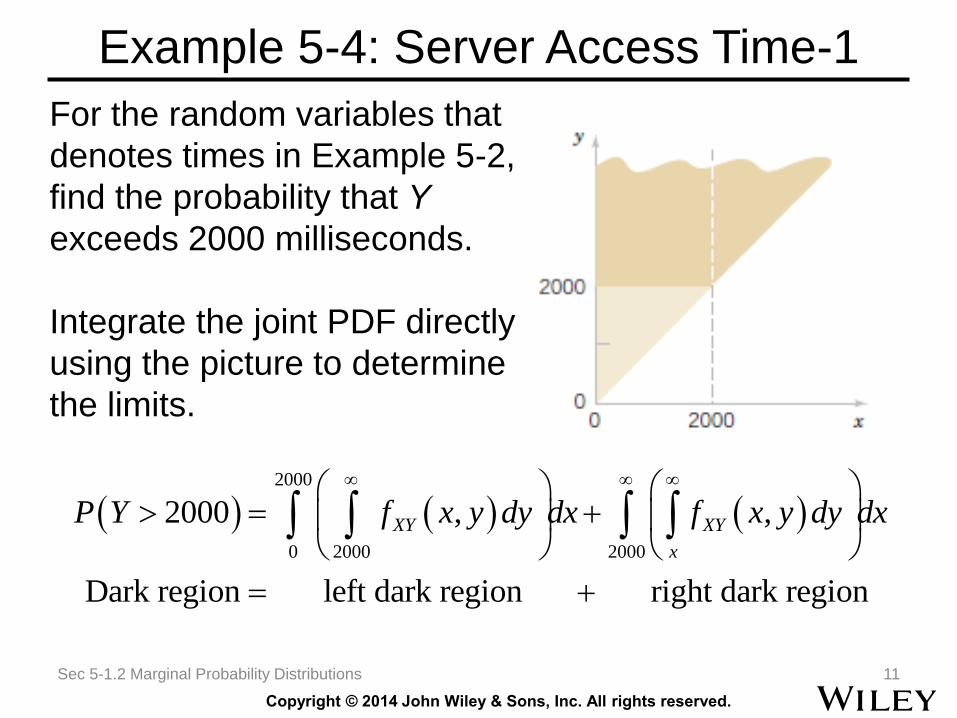
Example 5-4: Server Access Time-1
For the random variables that
denotes times in Example 5-2,
find the probability that Y
exceeds 2000 milliseconds.
Integrate the joint PDF directly
using the picture to determine
the limits.
Sec 5-1.2 Marginal Probability Distributions 11
2000
0 2000 2000
2000 , ,
Dark region left dark region right dark region
XY XY
x
P Y f x y dy dx f x y dy dx
Copyright © 2014 John Wiley & Sons, Inc. All rights reserved.
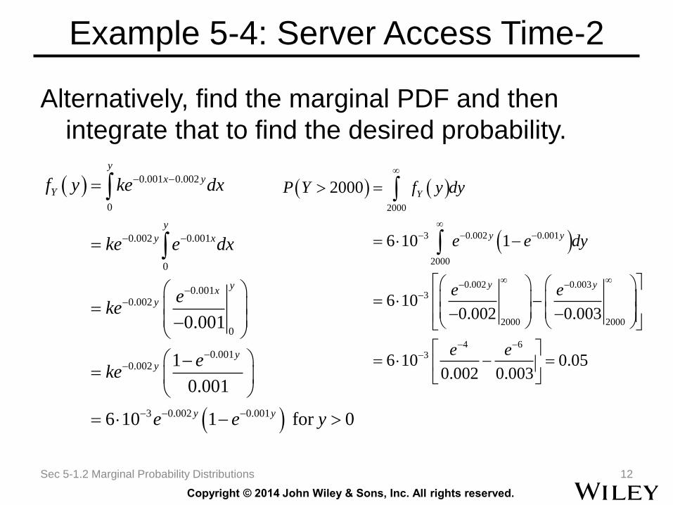
Example 5-4: Server Access Time-2
Alternatively, find the marginal PDF and then
integrate that to find the desired probability.
Sec 5-1.2 Marginal Probability Distributions 12
0.001 0.002
0
0.002 0.001
0
0.0010.002
0
0.0010.002
3 0.002 0.001
0.001
1
0.001
6 10 1 for 0
y
x y
Y
y
y x
yx
y
yy
y y
f y ke dx
ke e dx
eke
eke
e e y
2000
3 0.002 0.001
2000
0.002 0.0033
2000 2000
4 63
2000
6 10 1
6 100.002 0.003
6 10 0.050.002 0.003
Y
y y
y y
P Y f y dy
e e dy
e e
e e
Copyright © 2014 John Wiley & Sons, Inc. All rights reserved.
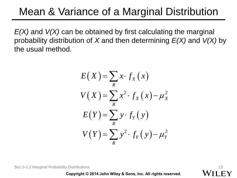
Mean & Variance of a Marginal Distribution
E(X) and V(X) can be obtained by first calculating the marginal
probability distribution of X and then determining E(X) and V(X) by
the usual method.
Sec 5-1.2 Marginal Probability Distributions 13
2 2
2 2
X
R
X X
R
Y
R
Y Y
R
E X x f x
V X x f x
E Y y f y
V Y y f y
Copyright © 2014 John Wiley & Sons, Inc. All rights reserved.
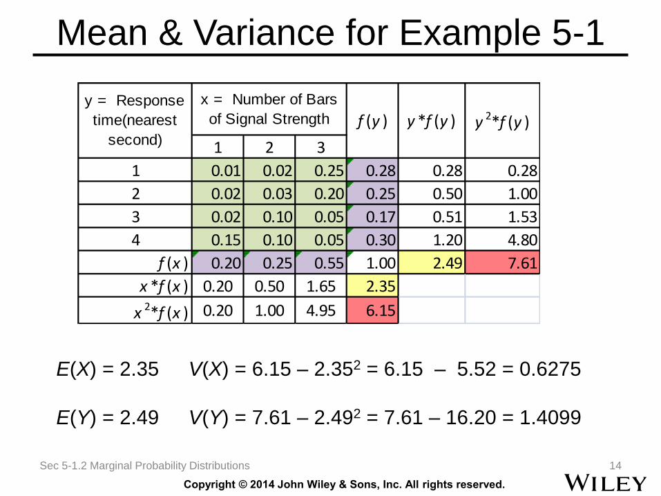
Mean & Variance for Example 5-1
Sec 5-1.2 Marginal Probability Distributions 14
1 2 3
1 0.01 0.02 0.25 0.28 0.28 0.28
2 0.02 0.03 0.20 0.25 0.50 1.00
3 0.02 0.10 0.05 0.17 0.51 1.53
4 0.15 0.10 0.05 0.30 1.20 4.80
f (x ) 0.20 0.25 0.55 1.00 2.49 7.61
x *f (x ) 0.20 0.50 1.65 2.35
x 2*f (x ) 0.20 1.00 4.95 6.15
y 2*f (y )
x = Number of Bars
of Signal Strength
y = Response
time(nearest
second)
f (y ) y *f (y )
E(X) = 2.35 V(X) = 6.15 – 2.352 = 6.15 – 5.52 = 0.6275
E(Y) = 2.49 V(Y) = 7.61 – 2.492 = 7.61 – 16.20 = 1.4099
Copyright © 2014 John Wiley & Sons, Inc. All rights reserved.
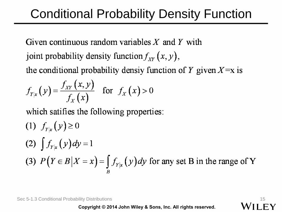
Conditional Probability Density Function
Sec 5-1.3 Conditional Probability Distributions 15
Copyright © 2014 John Wiley & Sons, Inc. All rights reserved.
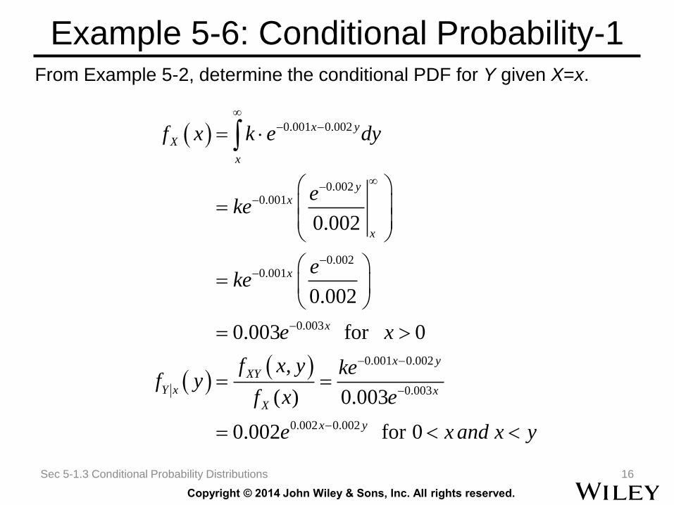
Example 5-6: Conditional Probability-1From Example 5-2, determine the conditional PDF for Y given X=x.
Sec 5-1.3 Conditional Probability Distributions 16
0.001 0.002
0.0020.001
0.0020.001
0.003
0.001 0.002
0.003
0.002 0.002
0.002
0.002
0.003 for 0
,
( ) 0.003
0.002 for 0
x y
X
x
yx
x
x
x
x yXY
Y x x
X
x y
f x k e dy
eke
eke
e x
f x y kef y
f x e
e x and x y
Copyright © 2014 John Wiley & Sons, Inc. All rights reserved.
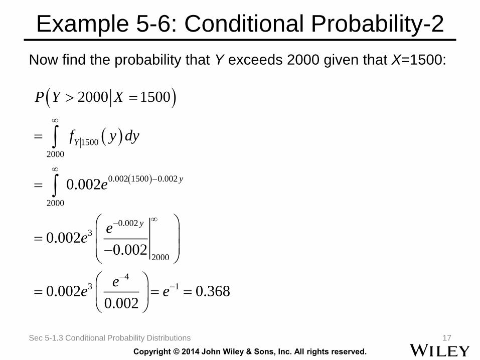
Example 5-6: Conditional Probability-2
Now find the probability that Y exceeds 2000 given that X=1500:
Sec 5-1.3 Conditional Probability Distributions 17
1500
2000
0.002 1500 0.002
2000
0.0023
2000
43 1
2000 1500
0.002
0.0020.002
0.002 0.3680.002
Y
y
y
P Y X
f y dy
e
ee
ee e
Copyright © 2014 John Wiley & Sons, Inc. All rights reserved.
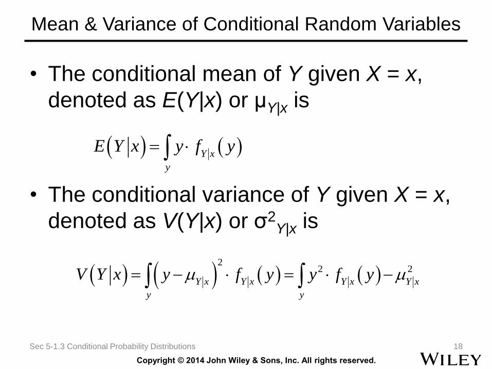
Mean & Variance of Conditional Random Variables
• The conditional mean of Y given X = x,
denoted as E(Y|x) or μY|x is
• The conditional variance of Y given X = x,
denoted as V(Y|x) or σ2Y|x is
Sec 5-1.3 Conditional Probability Distributions 18
Y x
y
E Y x y f y
2
2 2
Y x Y x Y x Y x
y y
V Y x y f y y f y
Copyright © 2014 John Wiley & Sons, Inc. All rights reserved.
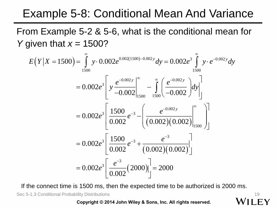
Example 5-8: Conditional Mean And Variance
From Example 5-2 & 5-6, what is the conditional mean for
Y given that x = 1500?
Sec 5-1.3 Conditional Probability Distributions 19
0.002 1500 0.002 3 0.002
1500 1500
0.002 0.0023
15001500
0.0023 3
1500
3
1500 0.002 0.002
0.0020.002 0.002
15000.002
0.002 0.002 0.002
0.002
y y
y y
y
E Y X y e dy e y e dy
e ee y dy
ee e
e
33
33
1500
0.002 0.002 0.002
0.002 2000 20000.002
ee
ee
If the connect time is 1500 ms, then the expected time to be authorized is 2000 ms.
Copyright © 2014 John Wiley & Sons, Inc. All rights reserved.
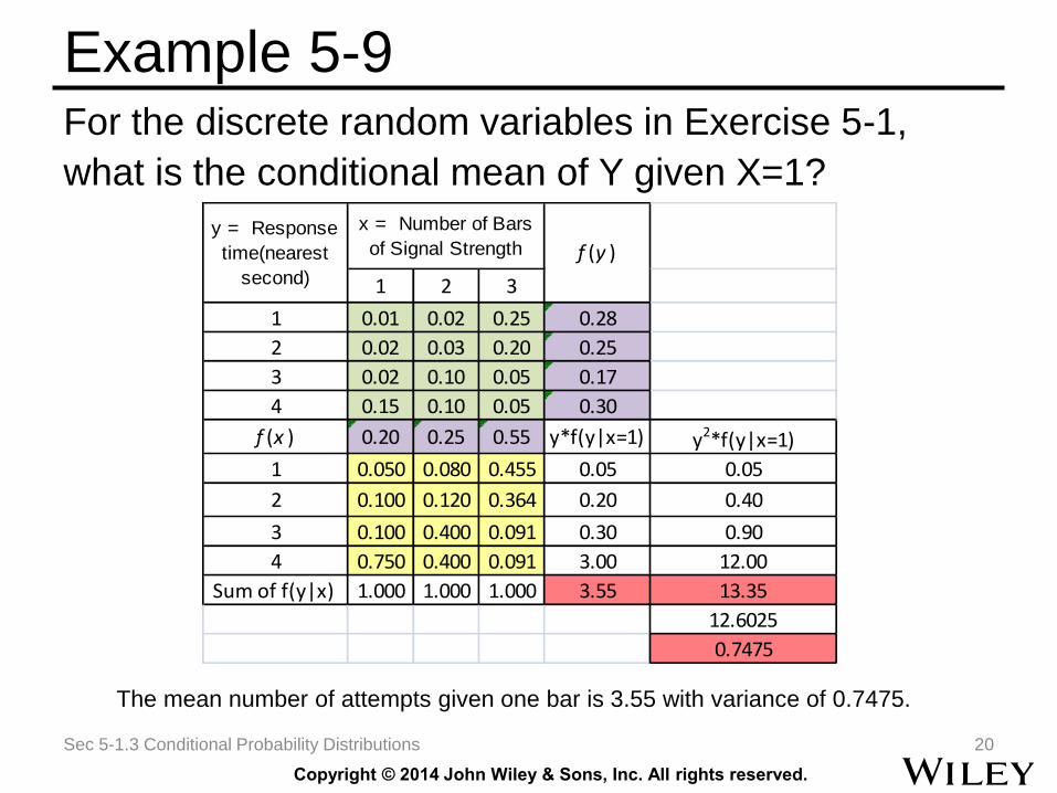
Example 5-9For the discrete random variables in Exercise 5-1,
what is the conditional mean of Y given X=1?
Sec 5-1.3 Conditional Probability Distributions 20
1 2 3
1 0.01 0.02 0.25 0.28
2 0.02 0.03 0.20 0.25
3 0.02 0.10 0.05 0.17
4 0.15 0.10 0.05 0.30
f (x ) 0.20 0.25 0.55 y*f(y|x=1) y2*f(y|x=1)
1 0.050 0.080 0.455 0.05 0.05
2 0.100 0.120 0.364 0.20 0.40
3 0.100 0.400 0.091 0.30 0.90
4 0.750 0.400 0.091 3.00 12.00
Sum of f(y|x) 1.000 1.000 1.000 3.55 13.35
12.6025
0.7475
f (y )y = Response
time(nearest
second)
x = Number of Bars
of Signal Strength
The mean number of attempts given one bar is 3.55 with variance of 0.7475.
Copyright © 2014 John Wiley & Sons, Inc. All rights reserved.
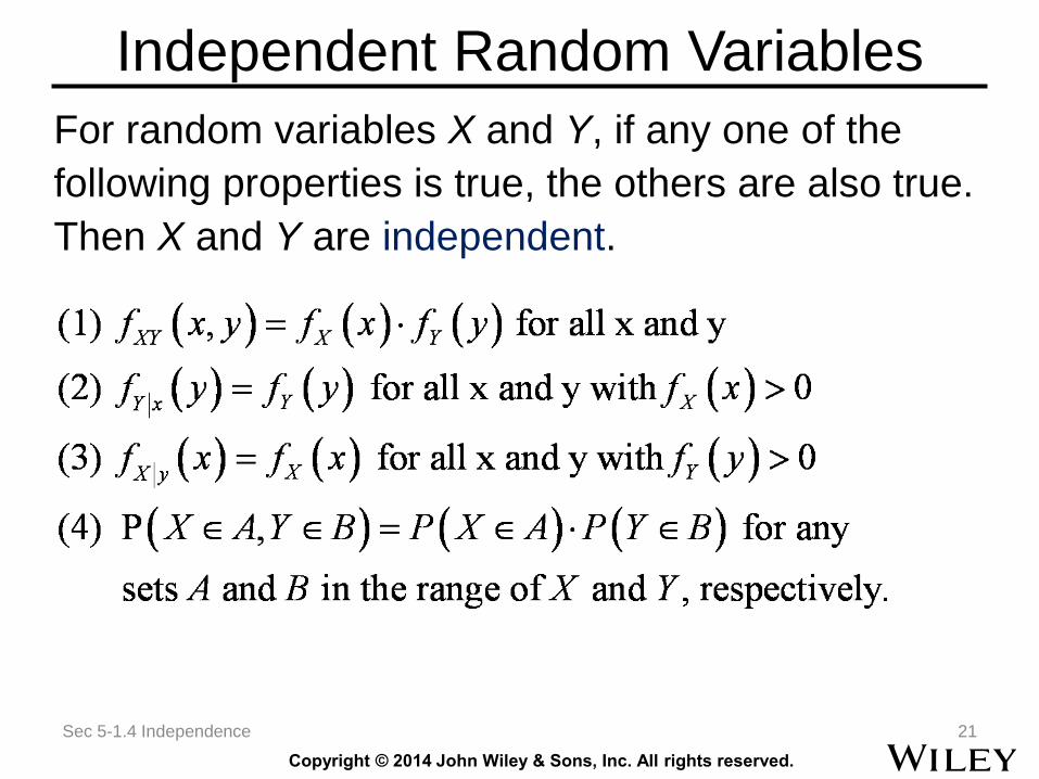
Independent Random Variables
For random variables X and Y, if any one of the
following properties is true, the others are also true.
Then X and Y are independent.
Sec 5-1.4 Independence 21
Copyright © 2014 John Wiley & Sons, Inc. All rights reserved.
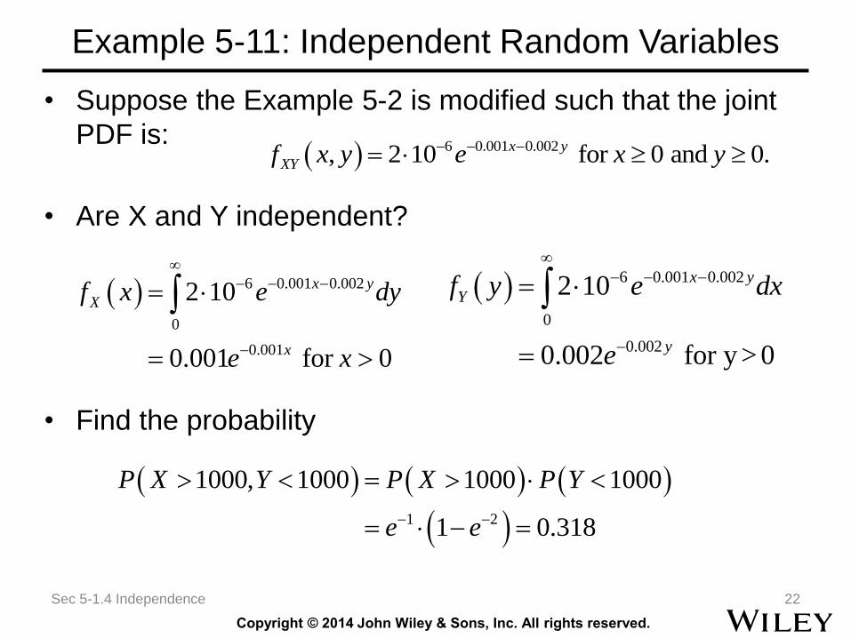
Example 5-11: Independent Random Variables
• Suppose the Example 5-2 is modified such that the joint
PDF is:
• Are X and Y independent?
• Find the probability
Sec 5-1.4 Independence 22
6 0.001 0.002, 2 10 for 0 and 0.x y
XYf x y e x y
6 0.001 0.002
0
0.001
2 10
0.001 for 0
x y
X
x
f x e dy
e x
6 0.001 0.002
0
0.002
2 10
0.002 for y > 0
x y
Y
y
f y e dx
e
1 2
1000, 1000 1000 1000
1 0.318
P X Y P X P Y
e e
Copyright © 2014 John Wiley & Sons, Inc. All rights reserved.
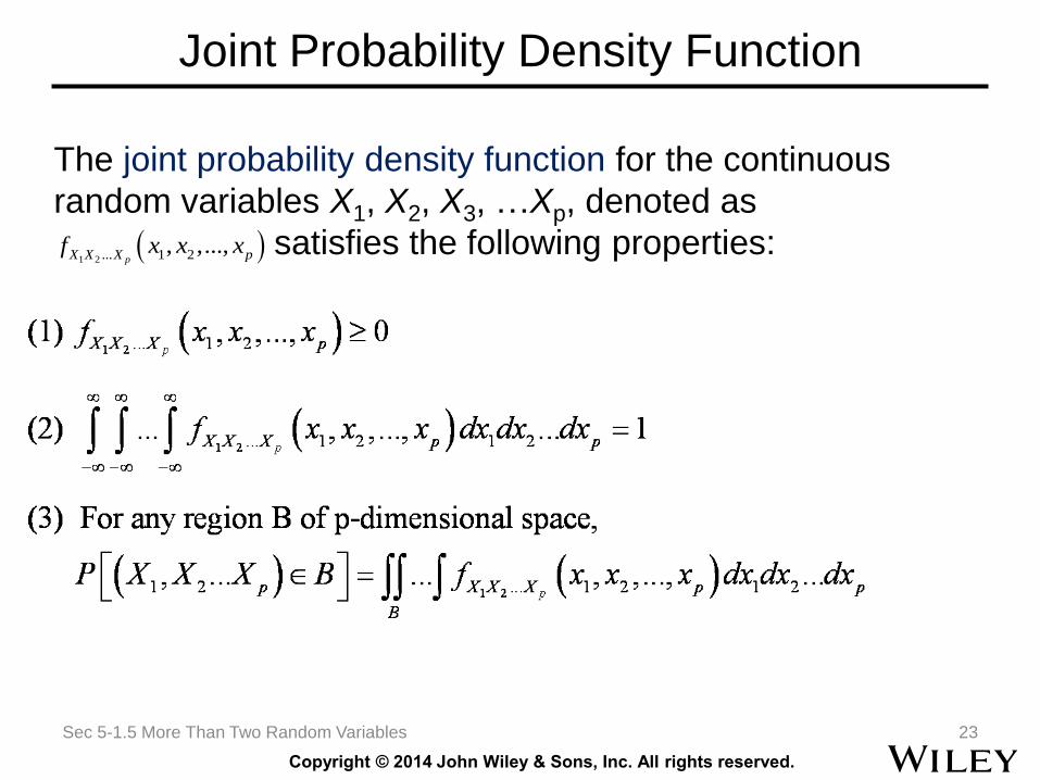
Joint Probability Density Function
Sec 5-1.5 More Than Two Random Variables 23
The joint probability density function for the continuous
random variables X1, X2, X3, …Xp, denoted as
satisfies the following properties: 1 2 ... 1 2, ,...,
pX X X pf x x x
Copyright © 2014 John Wiley & Sons, Inc. All rights reserved.
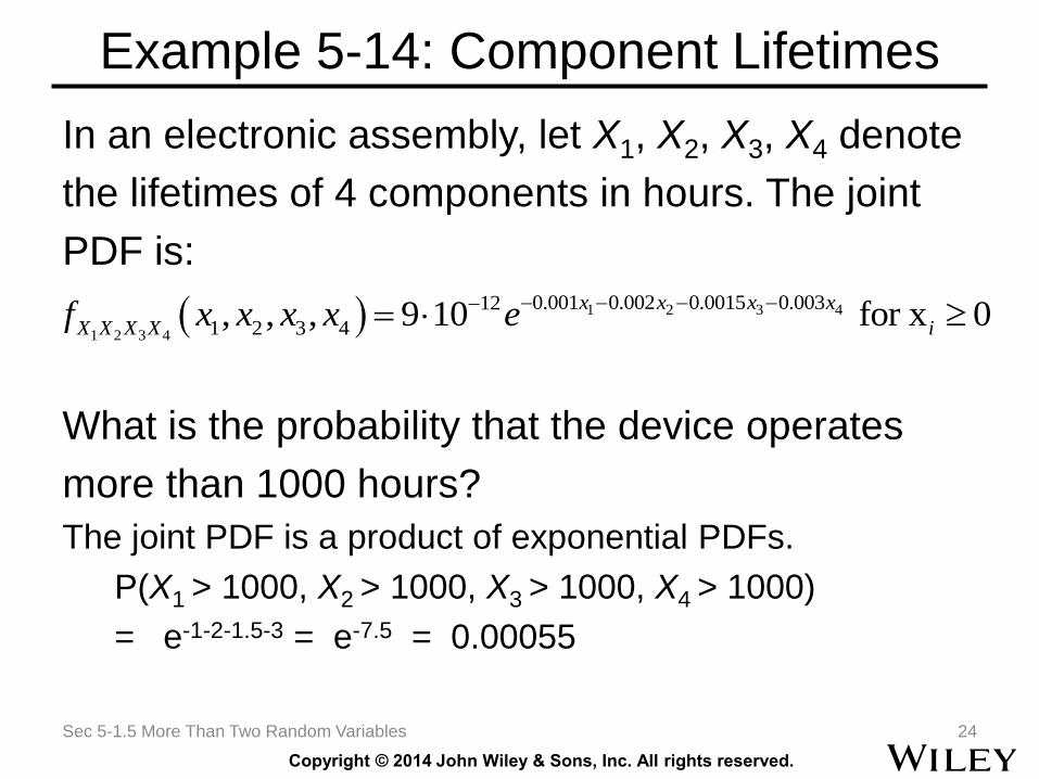
Example 5-14: Component Lifetimes
In an electronic assembly, let X1, X2, X3, X4 denote
the lifetimes of 4 components in hours. The joint
PDF is:
What is the probability that the device operates
more than 1000 hours?
The joint PDF is a product of exponential PDFs.
P(X1 > 1000, X2 > 1000, X3 > 1000, X4 > 1000)
= e-1-2-1.5-3 = e-7.5 = 0.00055
Sec 5-1.5 More Than Two Random Variables 24
1 2 3 4
1 2 3 4
0.001 0.002 0.0015 0.00312
1 2 3 4, , , 9 10 for x 0x x x x
X X X X if x x x x e
Copyright © 2014 John Wiley & Sons, Inc. All rights reserved.
Marginal Probability Density Function
Sec 5-1.5 More Than Two Random Variables 25
Copyright © 2014 John Wiley & Sons, Inc. All rights reserved.
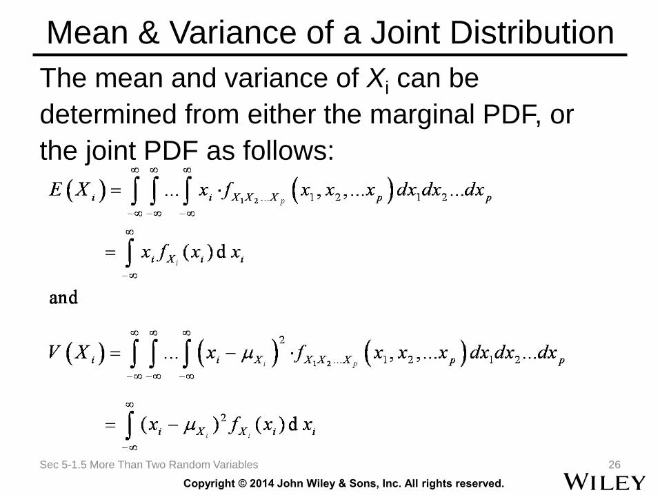
Mean & Variance of a Joint Distribution
The mean and variance of Xi can be
determined from either the marginal PDF, or
the joint PDF as follows:
Sec 5-1.5 More Than Two Random Variables 26
Copyright © 2014 John Wiley & Sons, Inc. All rights reserved.
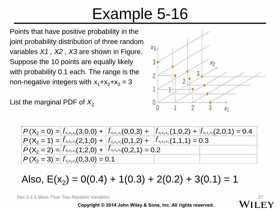
Example 5-16Points that have positive probability in the
joint probability distribution of three random
variables X1 , X2 , X3 are shown in Figure.
Suppose the 10 points are equally likely
with probability 0.1 each. The range is the
non-negative integers with x1+x2+x3 = 3
List the marginal PDF of X2
Sec 5-1.5 More Than Two Random Variables 27
P (X2 = 0) = (3,0,0) + (0,0,3) + (1,0,2) + (2,0,1) = 0.4
P (X2 = 1) = (2,1,0) + (0,1,2) + (1,1,1) = 0.3
P (X2 = 2) = (1,2,0) + (0,2,1) = 0.2
P (X2 = 3) = (0,3,0) = 0.1
321 xxxf 321 xxxf 321 xxxf 321 xxxf
321 xxxf321 xxxf 321 xxxf
321 xxxf 321 xxxf
321 xxxf
Also, E(x2) = 0(0.4) + 1(0.3) + 2(0.2) + 3(0.1) = 1
Copyright © 2014 John Wiley & Sons, Inc. All rights reserved.
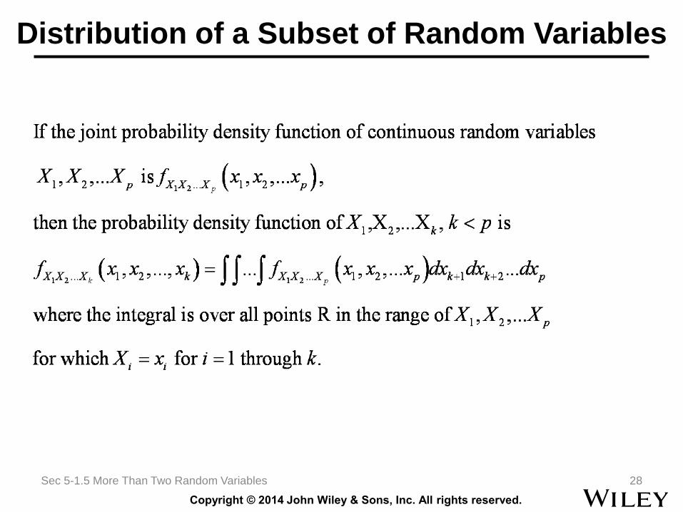
Distribution of a Subset of Random Variables
Sec 5-1.5 More Than Two Random Variables 28
Copyright © 2014 John Wiley & Sons, Inc. All rights reserved.
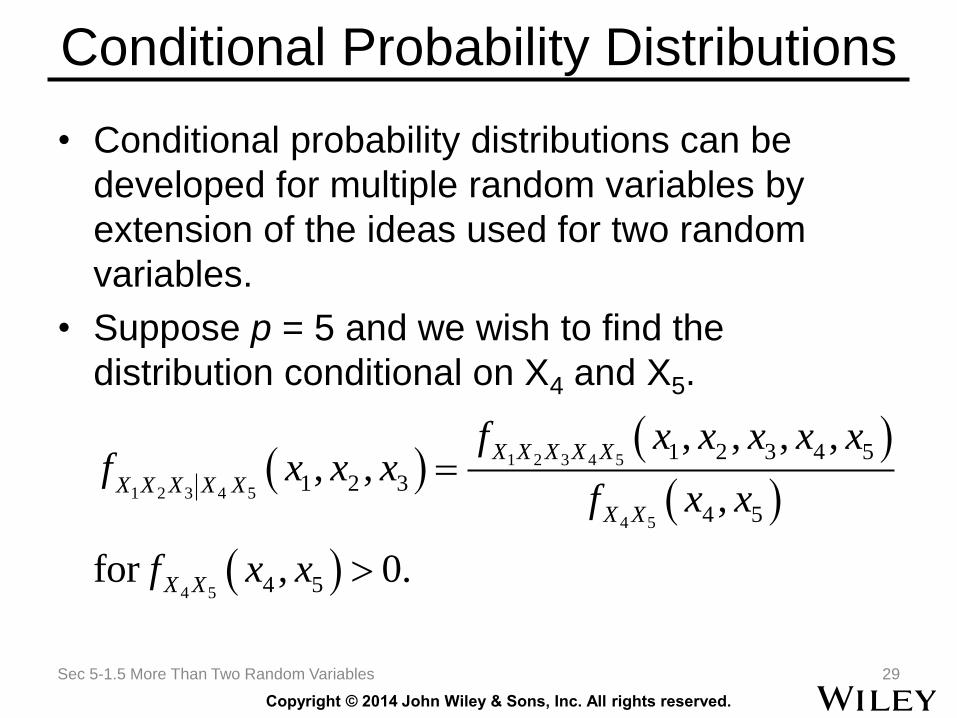
Conditional Probability Distributions
• Conditional probability distributions can be
developed for multiple random variables by
extension of the ideas used for two random
variables.
• Suppose p = 5 and we wish to find the
distribution conditional on X4 and X5.
Sec 5-1.5 More Than Two Random Variables 29
1 2 3 4 5
1 2 3 4 5
4 5
4 5
1 2 3 4 5
1 2 3
4 5
4 5
, , , ,, ,
,
for , 0.
X X X X X
X X X X X
X X
X X
f x x x x xf x x x
f x x
f x x
Copyright © 2014 John Wiley & Sons, Inc. All rights reserved.
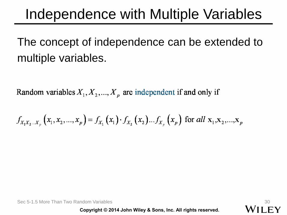
Independence with Multiple Variables
The concept of independence can be extended to
multiple variables.
Sec 5-1.5 More Than Two Random Variables 30
Copyright © 2014 John Wiley & Sons, Inc. All rights reserved.
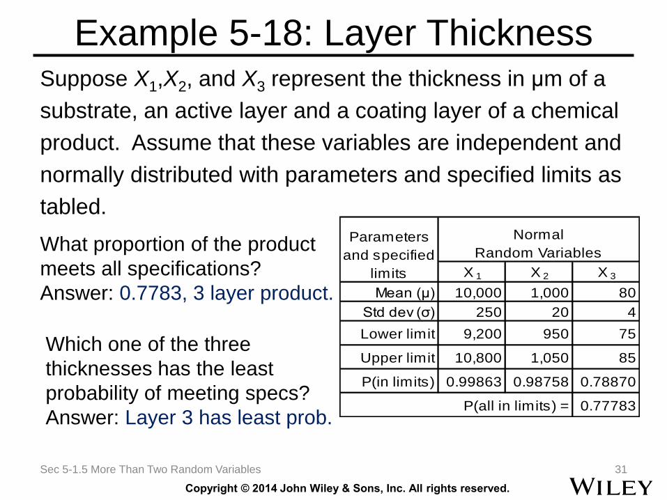
Example 5-18: Layer ThicknessSuppose X1,X2, and X3 represent the thickness in μm of a
substrate, an active layer and a coating layer of a chemical
product. Assume that these variables are independent and
normally distributed with parameters and specified limits as
tabled.
Sec 5-1.5 More Than Two Random Variables 31
X 1 X 2 X 3
Mean (μ) 10,000 1,000 80
Std dev (σ) 250 20 4
Lower limit 9,200 950 75
Upper limit 10,800 1,050 85
P(in limits) 0.99863 0.98758 0.78870
0.77783P(all in limits) =
Normal
Random VariablesParameters
and specified
limits
What proportion of the product
meets all specifications?
Answer: 0.7783, 3 layer product.
Which one of the three
thicknesses has the least
probability of meeting specs?
Answer: Layer 3 has least prob.
Copyright © 2014 John Wiley & Sons, Inc. All rights reserved.
Covariance
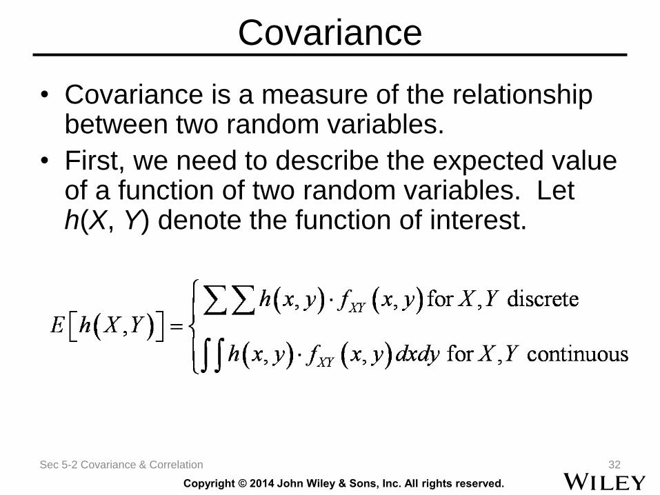
• Covariance is a measure of the relationship between two random variables.
• First, we need to describe the expected value of a function of two random variables. Let h(X, Y) denote the function of interest.
Sec 5-2 Covariance & Correlation 32
Copyright © 2014 John Wiley & Sons, Inc. All rights reserved.
Example 5-19: Expected Value of a Function of Two Random Variables
Sec 5-2 Covariance & Correlation 33
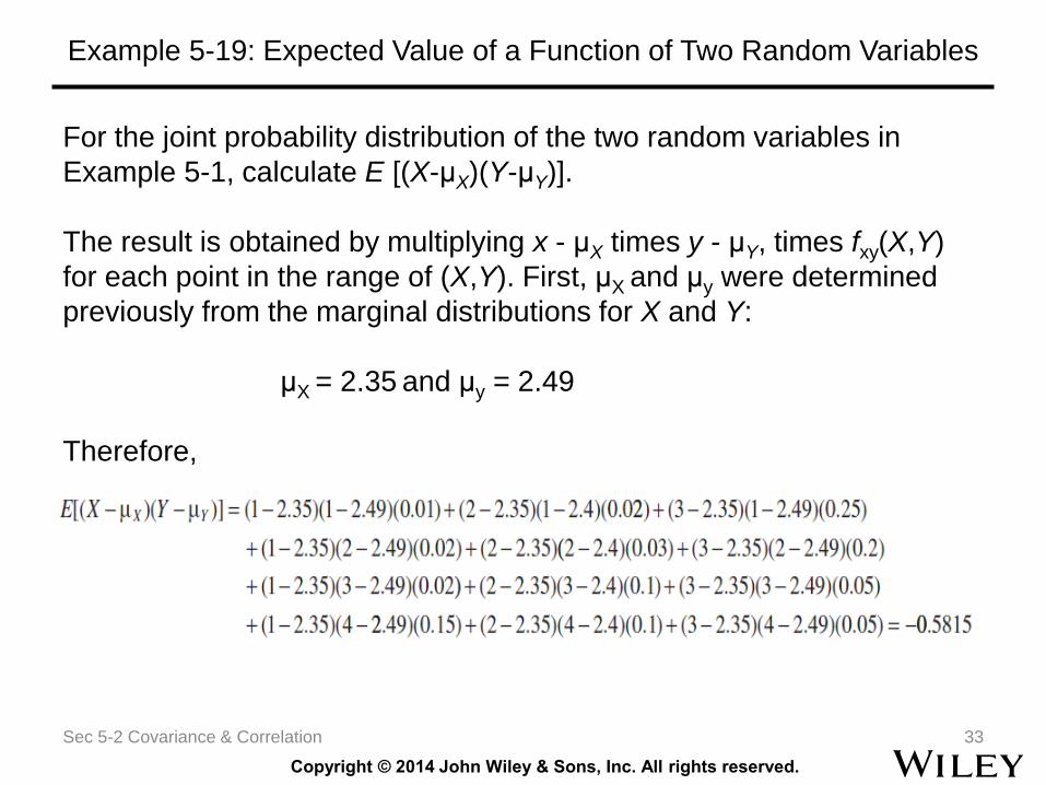
For the joint probability distribution of the two random variables in
Example 5-1, calculate E [(X-μX)(Y-μY)].
The result is obtained by multiplying x - μX times y - μY, times fxy(X,Y)
for each point in the range of (X,Y). First, μX and μy were determined
previously from the marginal distributions for X and Y:
μX = 2.35 and μy = 2.49
Therefore,
Copyright © 2014 John Wiley & Sons, Inc. All rights reserved.
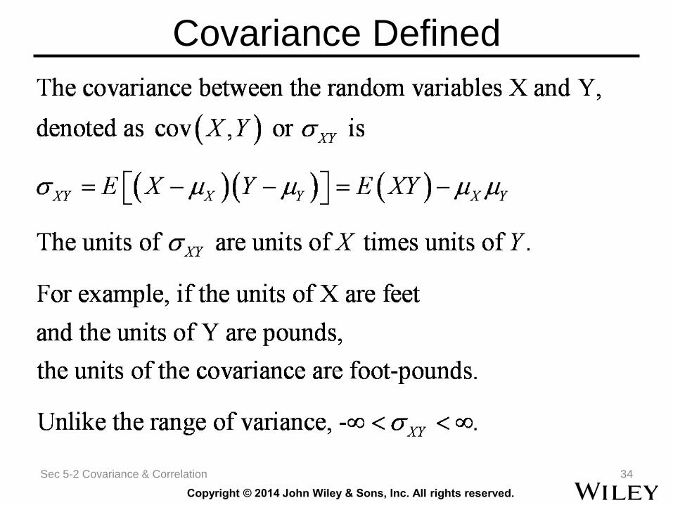
Covariance Defined
Sec 5-2 Covariance & Correlation 34
Copyright © 2014 John Wiley & Sons, Inc. All rights reserved.
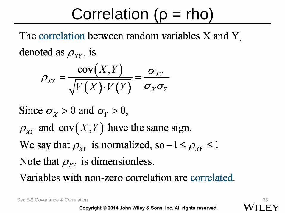
Correlation (ρ = rho)
Sec 5-2 Covariance & Correlation 35
Copyright © 2014 John Wiley & Sons, Inc. All rights reserved.
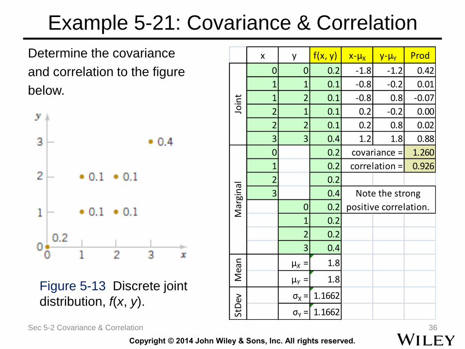
Example 5-21: Covariance & Correlation
Determine the covariance
and correlation to the figure
below.
Sec 5-2 Covariance & Correlation 36
x y f(x, y) x-μX y-μY Prod
0 0 0.2 -1.8 -1.2 0.42
1 1 0.1 -0.8 -0.2 0.01
1 2 0.1 -0.8 0.8 -0.07
2 1 0.1 0.2 -0.2 0.00
2 2 0.1 0.2 0.8 0.02
3 3 0.4 1.2 1.8 0.88
0 0.2 1.260
1 0.2 0.926
2 0.2
3 0.4
0 0.2
1 0.2
2 0.2
3 0.4
μX = 1.8
μY = 1.8
σX = 1.1662
σY = 1.1662StD
ev
correlation =
Mar
gin
al
covariance =
Mea
n
Note the strong
positive correlation.
Join
t
Figure 5-13 Discrete joint
distribution, f(x, y).
Copyright © 2014 John Wiley & Sons, Inc. All rights reserved.
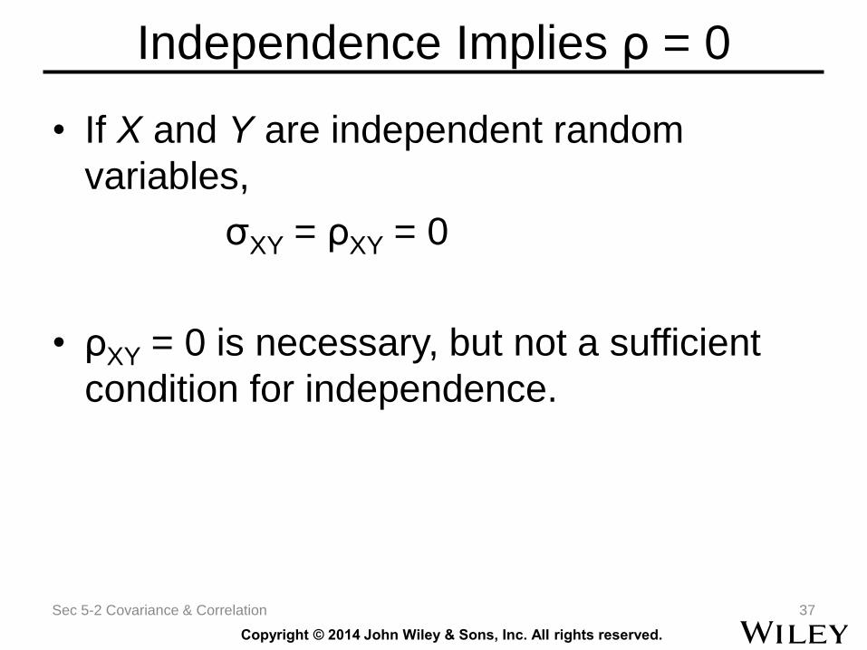
Independence Implies ρ = 0
• If X and Y are independent random
variables,
σXY = ρXY = 0
• ρXY = 0 is necessary, but not a sufficient
condition for independence.
Sec 5-2 Covariance & Correlation 37
Copyright © 2014 John Wiley & Sons, Inc. All rights reserved.
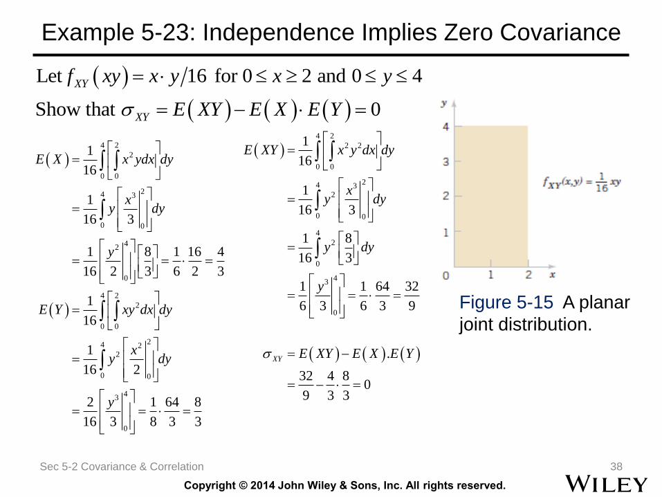
Example 5-23: Independence Implies Zero Covariance
Sec 5-2 Covariance & Correlation 38
Let 16 for 0 2 and 0 4
Show that 0
XY
XY
f xy x y x y
E XY E X E Y
Figure 5-15 A planar
joint distribution.
4 2
2 2
0 0
24 32
0 0
4
2
0
43
0
1
16
1
16 3
1 8
16 3
1 1 64 32
6 3 6 3 9
.
32 4 80
9 3 3
XY
E XY x y dx dy
xy dy
y dy
y
E XY E X E Y
4 2
2
0 0
24 3
0 0
42
0
4 2
2
0 0
24 22
0 0
43
0
1
16
1
16 3
1 8 1 16 4
16 2 3 6 2 3
1
16
1
16 2
2 1 64 8
16 3 8 3 3
E X x ydx dy
xy dy
y
E Y xy dx dy
xy dy
y
Copyright © 2014 John Wiley & Sons, Inc. All rights reserved.
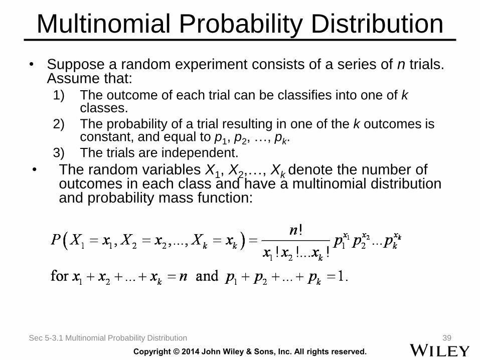
Multinomial Probability Distribution
• Suppose a random experiment consists of a series of n trials. Assume that:1) The outcome of each trial can be classifies into one of k
classes.
2) The probability of a trial resulting in one of the k outcomes is constant, and equal to p1, p2, …, pk.
3) The trials are independent.
• The random variables X1, X2,…, Xk denote the number of outcomes in each class and have a multinomial distribution and probability mass function:
Sec 5-3.1 Multinomial Probability Distribution 39
Copyright © 2014 John Wiley & Sons, Inc. All rights reserved.
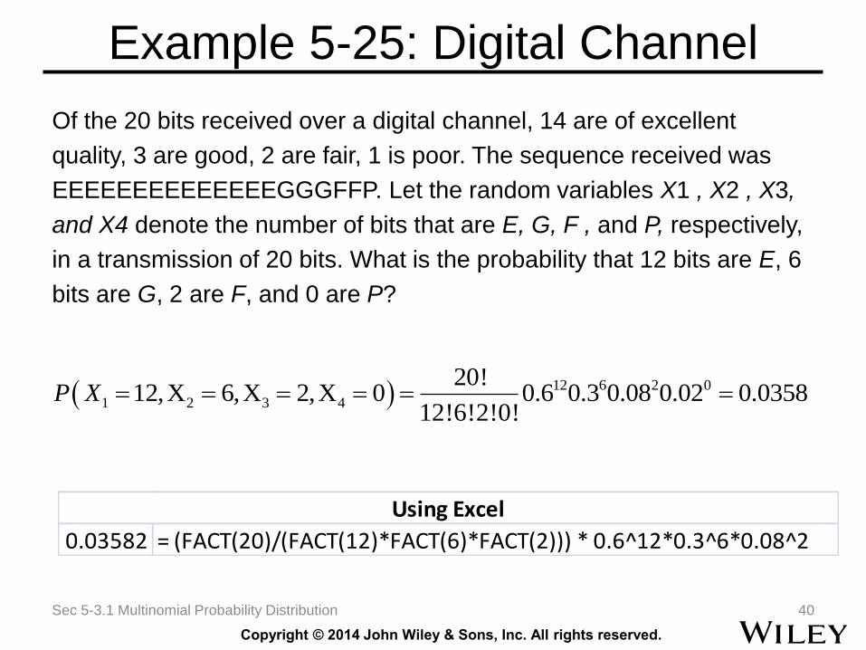
Example 5-25: Digital Channel
Of the 20 bits received over a digital channel, 14 are of excellent
quality, 3 are good, 2 are fair, 1 is poor. The sequence received was
EEEEEEEEEEEEEEGGGFFP. Let the random variables X1 , X2 , X3,
and X4 denote the number of bits that are E, G, F , and P, respectively,
in a transmission of 20 bits. What is the probability that 12 bits are E, 6
bits are G, 2 are F, and 0 are P?
Sec 5-3.1 Multinomial Probability Distribution 40
12 6 2 0
1 2 3 4
20!12,X 6,X 2,X 0 0.6 0.3 0.08 0.02 0.0358
12!6!2!0!P X
0.03582 = (FACT(20)/(FACT(12)*FACT(6)*FACT(2))) * 0.6^12*0.3^6*0.08^2
Using Excel
Copyright © 2014 John Wiley & Sons, Inc. All rights reserved.
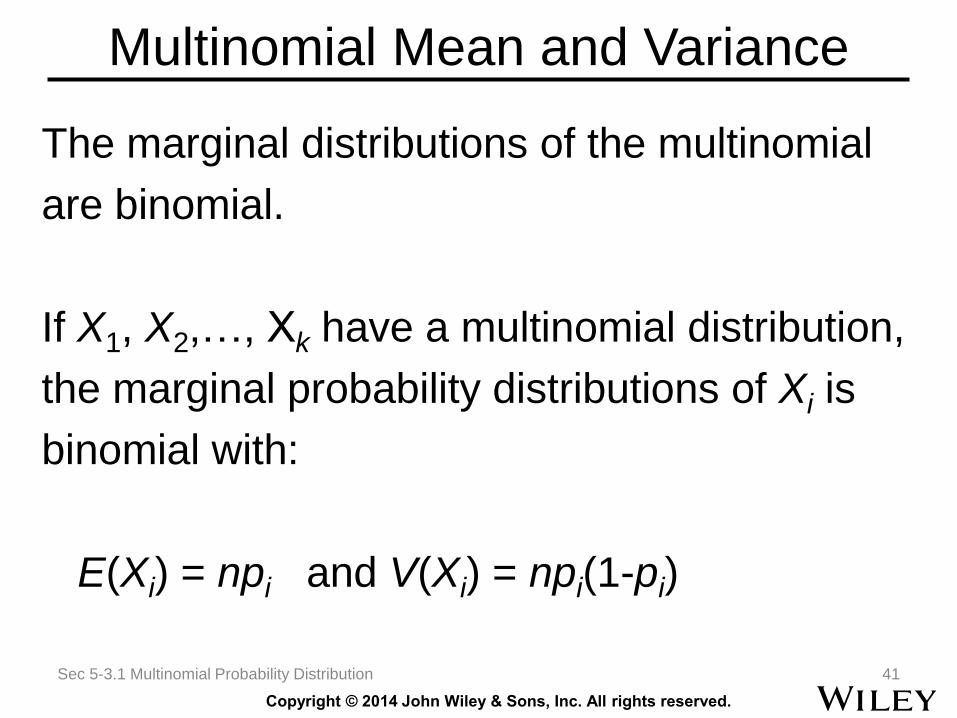
Multinomial Mean and Variance
The marginal distributions of the multinomial
are binomial.
If X1, X2,…, Xk have a multinomial distribution,
the marginal probability distributions of Xi is
binomial with:
E(Xi) = npi and V(Xi) = npi(1-pi)
Sec 5-3.1 Multinomial Probability Distribution 41
Copyright © 2014 John Wiley & Sons, Inc. All rights reserved.
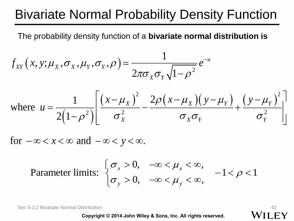
Bivariate Normal Probability Density Function
Sec 5-3.2 Bivariate Normal Distribution 42
2
2 2
2 22
1, ; , , , ,
2 1
21where
2 1
for and .
u
XY X X Y Y
X Y
X X Y Y
X X Y Y
f x y e
x x y yu
x y
0, ,Parameter limits: 1 1
0, ,
x x
y y
The probability density function of a bivariate normal distribution is
Copyright © 2014 John Wiley & Sons, Inc. All rights reserved.
Marginal Distributions of the Bivariate Normal Random Variables
If X and Y have a bivariate normal distribution with
joint probability density function
fXY(x,y;σX,σY,μX,μY,ρ)
the marginal probability distributions of X and Y
are normal with means μX and μY and standard
deviations σX and σY, respectively.
Sec 5-3.2 Bivariate Normal Distribution 43
Copyright © 2014 John Wiley & Sons, Inc. All rights reserved.
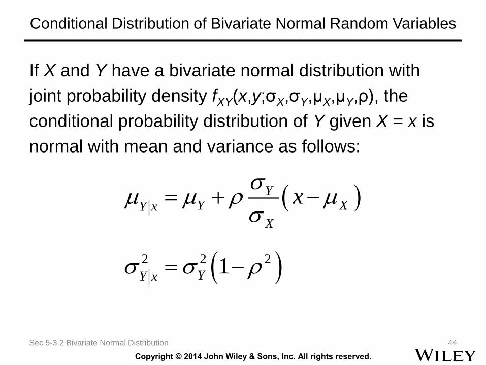
Conditional Distribution of Bivariate Normal Random Variables
If X and Y have a bivariate normal distribution with
joint probability density fXY(x,y;σX,σY,μX,μY,ρ), the
conditional probability distribution of Y given X = x is
normal with mean and variance as follows:
Sec 5-3.2 Bivariate Normal Distribution 44
2 2 21
YY XY x
X
YY x
x
Copyright © 2014 John Wiley & Sons, Inc. All rights reserved.
Correlation of Bivariate Normal Random Variables
If X and Y have a bivariate normal
distribution with joint probability density
function fXY(x,y;σX,σY,μX,μY,ρ), the
correlation between X and Y is ρ.
Sec 5-3.2 Bivariate Normal Distribution 45
Copyright © 2014 John Wiley & Sons, Inc. All rights reserved.
Bivariate Normal Correlation and Independence
• In general, zero correlation does not imply independence.
• But in the special case that X and Y have a bivariate normal distribution, if ρ = 0, then X and Y are independent.
If X and Y have a bivariate normal
distribution with ρ=0, X and Y are
independent.
Sec 5-3.2 Bivariate Normal Distribution 46
Copyright © 2014 John Wiley & Sons, Inc. All rights reserved.
Linear Functions of Random Variables
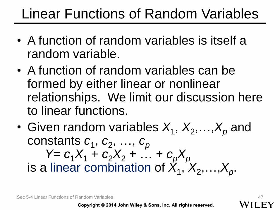
• A function of random variables is itself a random variable.
• A function of random variables can be formed by either linear or nonlinear relationships. We limit our discussion here to linear functions.
• Given random variables X1, X2,…,Xp and constants c1, c2, …, cp
Y= c1X1 + c2X2 + … + cpXp
is a linear combination of X1, X2,…,Xp.
Sec 5-4 Linear Functions of Random Variables 47
Copyright © 2014 John Wiley & Sons, Inc. All rights reserved.
Mean and Variance of a Linear Function
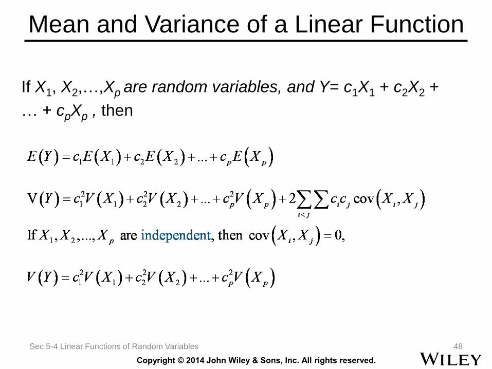
If X1, X2,…,Xp are random variables, and Y= c1X1 + c2X2 +
… + cpXp , then
Sec 5-4 Linear Functions of Random Variables 48
Copyright © 2014 John Wiley & Sons, Inc. All rights reserved.
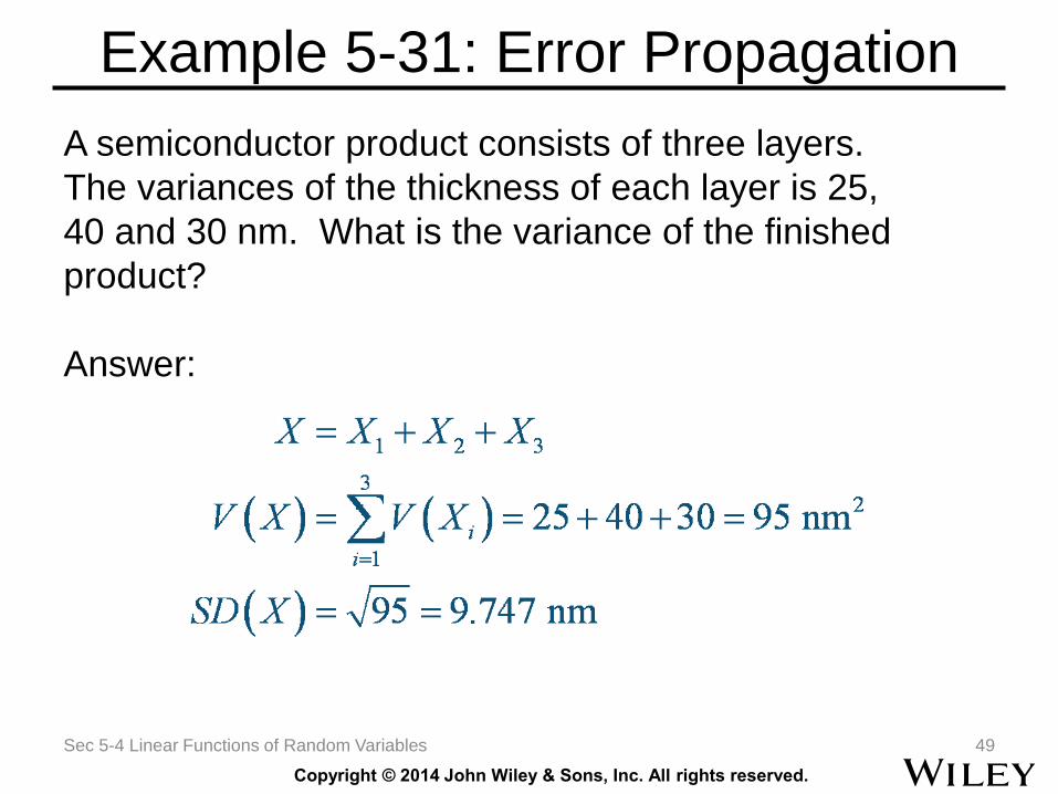
Example 5-31: Error Propagation
A semiconductor product consists of three layers.
The variances of the thickness of each layer is 25,
40 and 30 nm. What is the variance of the finished
product?
Answer:
Sec 5-4 Linear Functions of Random Variables 49
Copyright © 2014 John Wiley & Sons, Inc. All rights reserved.
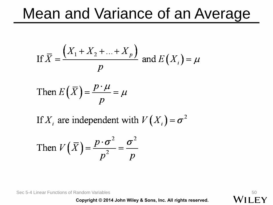
Mean and Variance of an Average
Sec 5-4 Linear Functions of Random Variables 50
Copyright © 2014 John Wiley & Sons, Inc. All rights reserved.
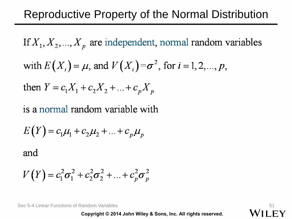
Reproductive Property of the Normal Distribution
Sec 5-4 Linear Functions of Random Variables 51
Copyright © 2014 John Wiley & Sons, Inc. All rights reserved.
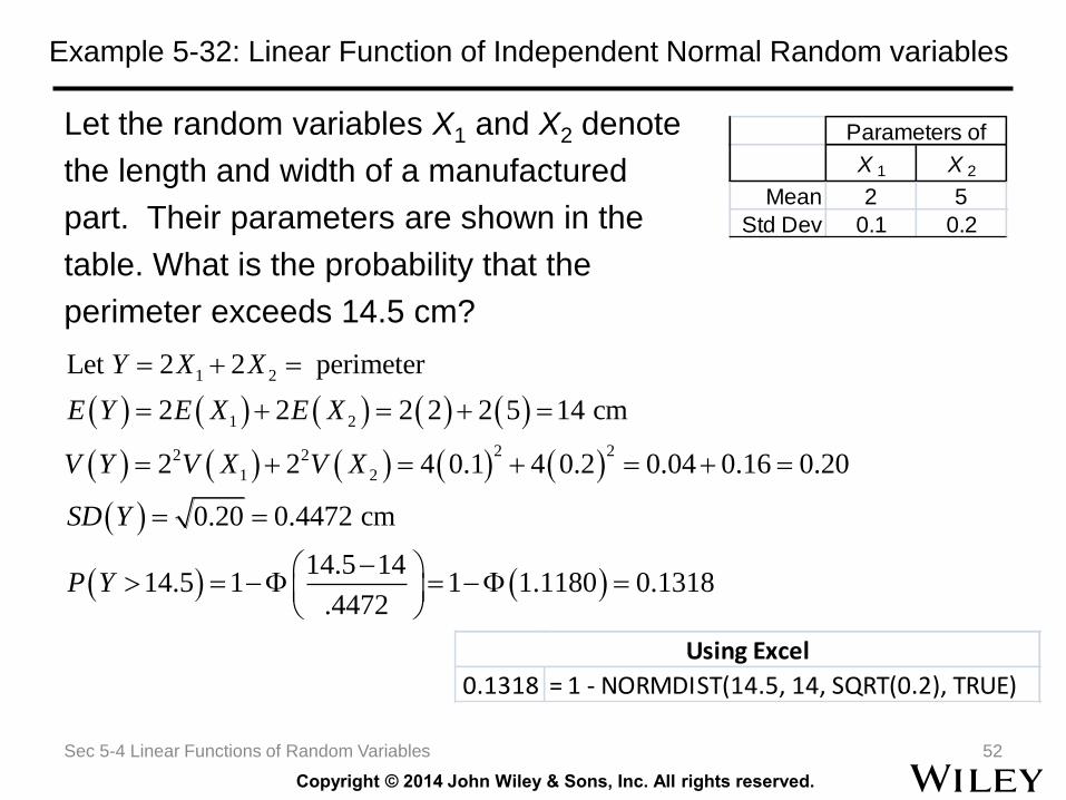
Example 5-32: Linear Function of Independent Normal Random variables
Let the random variables X1 and X2 denote
the length and width of a manufactured
part. Their parameters are shown in the
table. What is the probability that the
perimeter exceeds 14.5 cm?
Sec 5-4 Linear Functions of Random Variables 52
X 1 X 2
Mean 2 5
Std Dev 0.1 0.2
Parameters of
1 2
1 2
2 22 2
1 2
Let 2 2 perimeter
2 2 2 2 2 5 14 cm
2 2 4 0.1 4 0.2 0.04 0.16 0.20
0.20 0.4472 cm
14.5 1414.5 1 1 1.1180 0.1318
.4472
Y X X
E Y E X E X
V Y V X V X
SD Y
P Y
0.1318 = 1 - NORMDIST(14.5, 14, SQRT(0.2), TRUE)
Using Excel
Copyright © 2014 John Wiley & Sons, Inc. All rights reserved.
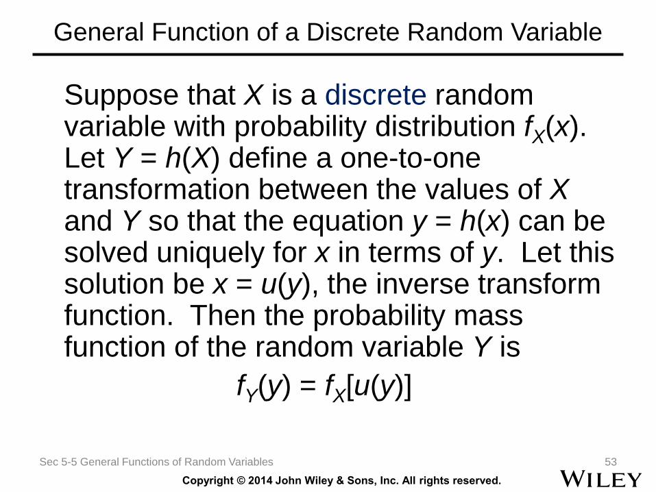
General Function of a Discrete Random Variable
Suppose that X is a discrete random variable with probability distribution fX(x). Let Y = h(X) define a one-to-one transformation between the values of Xand Y so that the equation y = h(x) can be solved uniquely for x in terms of y. Let this solution be x = u(y), the inverse transform function. Then the probability mass function of the random variable Y is
fY(y) = fX[u(y)]
Sec 5-5 General Functions of Random Variables 53
Copyright © 2014 John Wiley & Sons, Inc. All rights reserved.
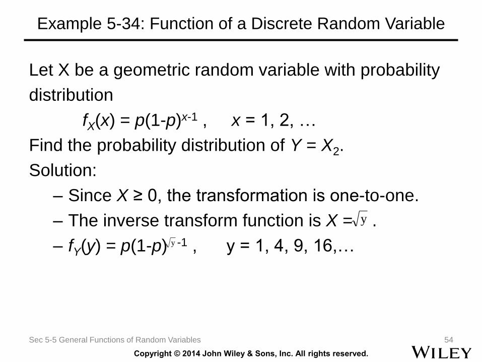
Example 5-34: Function of a Discrete Random Variable
Let X be a geometric random variable with probability
distribution
fX(x) = p(1-p)x-1 , x = 1, 2, …
Find the probability distribution of Y = X2.
Solution:
– Since X ≥ 0, the transformation is one-to-one.
– The inverse transform function is X = .
– fY(y) = p(1-p) -1 , y = 1, 4, 9, 16,…
Sec 5-5 General Functions of Random Variables 54
y
y
Copyright © 2014 John Wiley & Sons, Inc. All rights reserved.
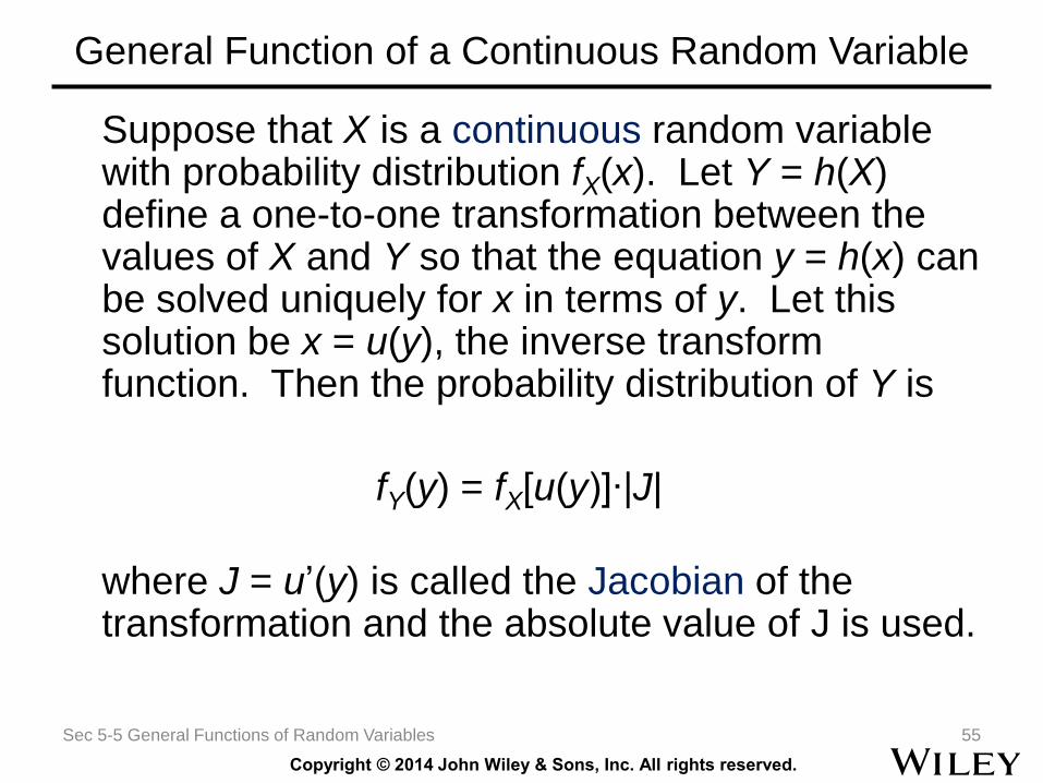
General Function of a Continuous Random Variable
Suppose that X is a continuous random variable with probability distribution fX(x). Let Y = h(X) define a one-to-one transformation between the values of X and Y so that the equation y = h(x) can be solved uniquely for x in terms of y. Let this solution be x = u(y), the inverse transform function. Then the probability distribution of Y is
fY(y) = fX[u(y)]∙|J|
where J = u’(y) is called the Jacobian of the transformation and the absolute value of J is used.
Sec 5-5 General Functions of Random Variables 55
Copyright © 2014 John Wiley & Sons, Inc. All rights reserved.
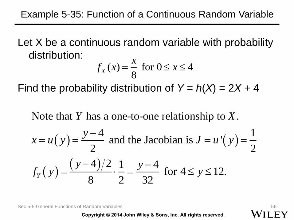
Example 5-35: Function of a Continuous Random Variable
Let X be a continuous random variable with probability
distribution:
Find the probability distribution of Y = h(X) = 2X + 4
Sec 5-5 General Functions of Random Variables 56
( ) for 0 48
X
xf x x
Note that has a one-to-one relationship to .
4 1 and the Jacobian is '
2 2
4 2 1 4 for 4 12.
8 2 32Y
Y X
yx u y J u y
y yf y y
Copyright © 2014 John Wiley & Sons, Inc. All rights reserved.
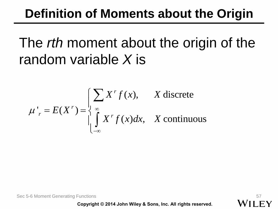
Definition of Moments about the Origin
Sec 5-6 Moment Generating Functions 57
The rth moment about the origin of the
random variable X is
( ), discrete
' ( )( ) , continuous
r
r
r r
X f x X
E XX f x dx X
Copyright © 2014 John Wiley & Sons, Inc. All rights reserved.
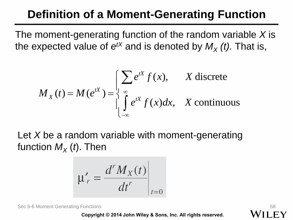
Definition of a Moment-Generating Function
Sec 5-6 Moment Generating Functions 58
The moment-generating function of the random variable X is
the expected value of etX and is denoted by MX (t). That is,
( ), discrete
( ) ( )( ) , continuous
tX
tX
X tX
e f x X
M t M ee f x dx X
Let X be a random variable with moment-generating
function MX (t). Then
Copyright © 2014 John Wiley & Sons, Inc. All rights reserved.
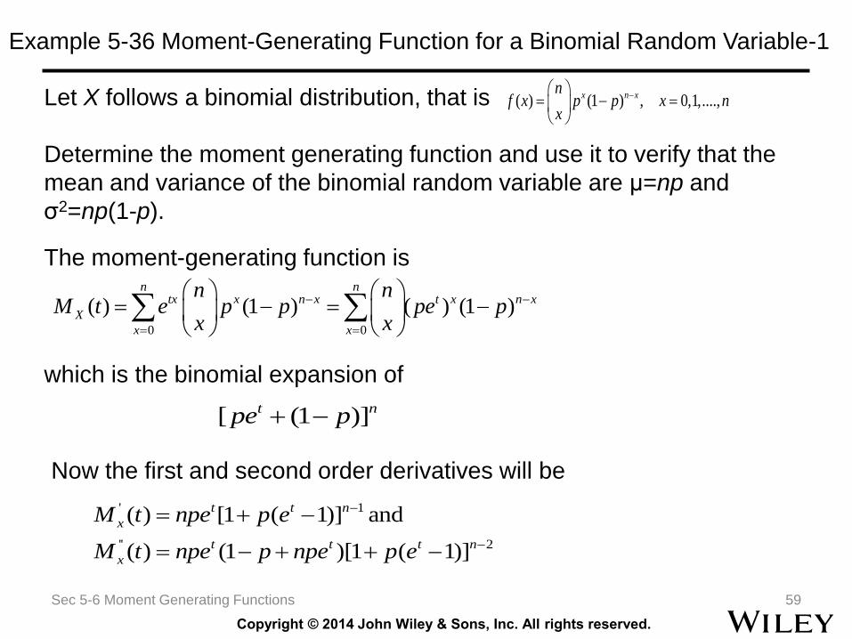
Example 5-36 Moment-Generating Function for a Binomial Random Variable-1
Sec 5-6 Moment Generating Functions 59
Let X follows a binomial distribution, that is
Determine the moment generating function and use it to verify that the
mean and variance of the binomial random variable are μ=np and
σ2=np(1-p).
( ) (1 ) , 0,1,....,x n xn
f x p p x nx
Now the first and second order derivatives will be
0 0
( ) (1 ) ( ) (1 )n n
tx x n x t x n x
X
x x
n nM t e p p pe p
x x
The moment-generating function is
which is the binomial expansion of
[ (1 )]t npe p
' 1
'' 2
( ) [1 ( 1)] and
( ) (1 )[1 ( 1)]
t t n
x
t t t n
x
M t npe p e
M t npe p npe p e
Copyright © 2014 John Wiley & Sons, Inc. All rights reserved.
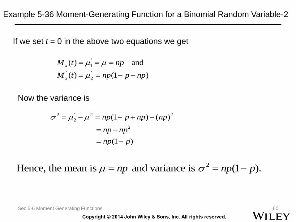
Example 5-36 Moment-Generating Function for a Binomial Random Variable-2
Sec 5-6 Moment Generating Functions 60
If we set t = 0 in the above two equations we get
' '
1
'' '
2
( ) and
( ) (1 )
x
x
M t np
M t np p np
Now the variance is
2 ' 2 2
2
2
(1 ) ( )
(1 )
np p np np
np np
np p
2Hence, the mean is and variance is (1 ).np np p
Copyright © 2014 John Wiley & Sons, Inc. All rights reserved.
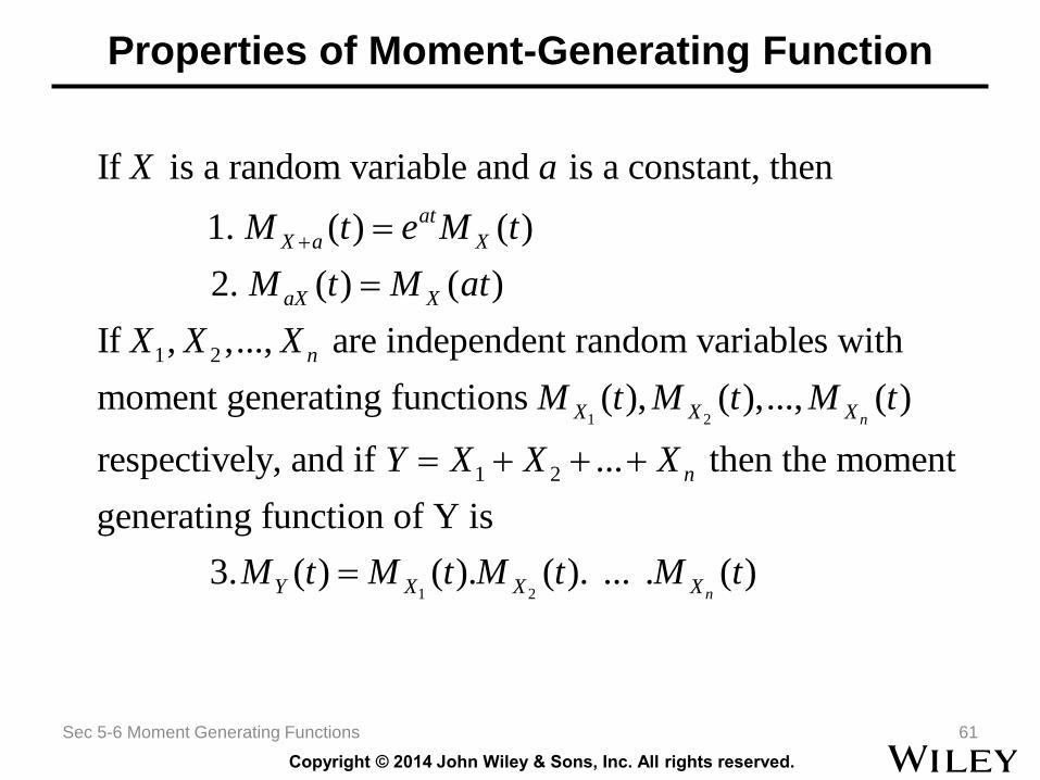
Properties of Moment-Generating Function
Sec 5-6 Moment Generating Functions 61
1 2
1 2
1. ( ) ( )
2. ( ) ( )
If , ,..., are independent random vari
If is a random variable
ables with
moment generat
and is a co
ing functions ( ), ( ),...,
nstant, then
( )
respectiv
n
at
X a X
aX X
n
X X X
M t e M t
M t M at
X X X
M t M t M t
X a
1 2
1 2ely, and if ... then the moment
generating function of Y is
3. ( ) ( ). ( ). ... . ( )n
n
Y X X X
Y X X X
M t M t M t M t
Copyright © 2014 John Wiley & Sons, Inc. All rights reserved.
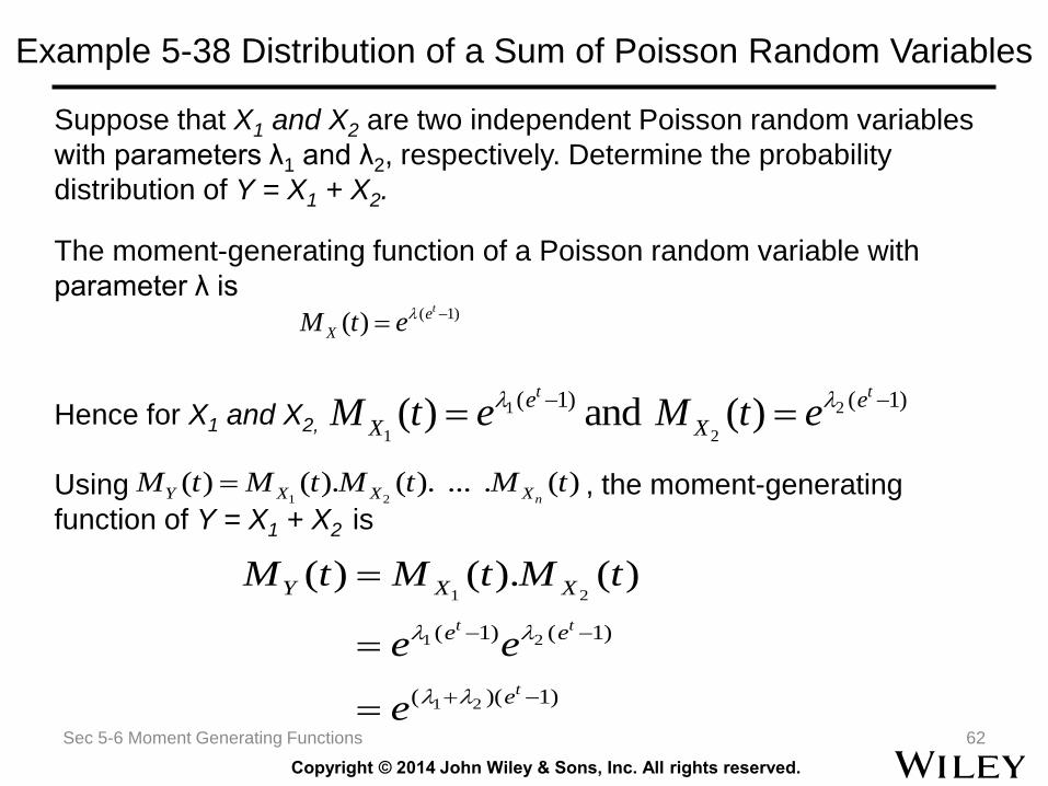
Example 5-38 Distribution of a Sum of Poisson Random Variables
Sec 5-6 Moment Generating Functions 62
Suppose that X1 and X2 are two independent Poisson random variables
with parameters λ1 and λ2, respectively. Determine the probability
distribution of Y = X1 + X2.
Using , the moment-generating
function of Y = X1 + X2 is
( 1)( )te
XM t e
The moment-generating function of a Poisson random variable with
parameter λ is
Hence for X1 and X2,1 2
1 2
( 1) ( 1)( ) and ( )
t te e
X XM t e M t e
1 2
1 2
1 2
( 1) ( 1)
( )( 1)
( ) ( ). ( )
t t
t
Y X X
e e
e
M t M t M t
e e
e
1 2( ) ( ). ( ). ... . ( )
nY X X XM t M t M t M t
Copyright © 2014 John Wiley & Sons, Inc. All rights reserved.
Important Terms & Concepts for Chapter 5
Bivariate distribution
Bivariate normal distribution
Conditional mean
Conditional probability density
function
Conditional probability mass
function
Conditional variance
Contour plots
Correlation
Covariance
Error propagation
General functions of random
variables
Independence
Joint probability density function
Joint probability mass function
Linear functions of random
variables
Marginal probability distribution
Multinomial distribution
Reproductive property of the
normal distribution
Chapter 5 Summary 63