Probability Basics for Machine Learningurtasun/courses/CSC411/tutorial1.pdf · Joint and...

Probability Theory for Machine Learning

Chris Cremer

September 2015

Outline

• Motivation

• Probability Definitions and Rules

• Probability Distributions

• MLE for Gaussian Parameter Estimation

• MLE and Least Squares

Material

• Pattern Recognition and Machine Learning - Christopher M. Bishop

• All of Statistics – Larry Wasserman

• Wolfram MathWorld

• Wikipedia

Motivation

• Uncertainty arises through:• Noisy measurements

• Finite size of data sets

• Ambiguity: The word bank can mean (1) a financial institution, (2) the side of a river, or (3) tilting an airplane. Which meaning was intended, based on the words that appear nearby?

• Limited Model Complexity

• Probability theory provides a consistent framework for the quantification and manipulation of uncertainty

• Allows us to make optimal predictions given all the information available to us, even though that information may be incomplete or ambiguous

Sample Space

• The sample space Ω is the set of possible outcomes of an experiment. Points ω in Ω are called sample outcomes, realizations, or elements. Subsets of Ω are called Events.

• Example. If we toss a coin twice then Ω = {HH,HT, TH, TT}. The event that the first toss is heads is A = {HH,HT}

• We say that events A1 and A2 are disjoint (mutually exclusive) if Ai ∩Aj = {}• Example: first flip being heads and first flip being tails

Probability

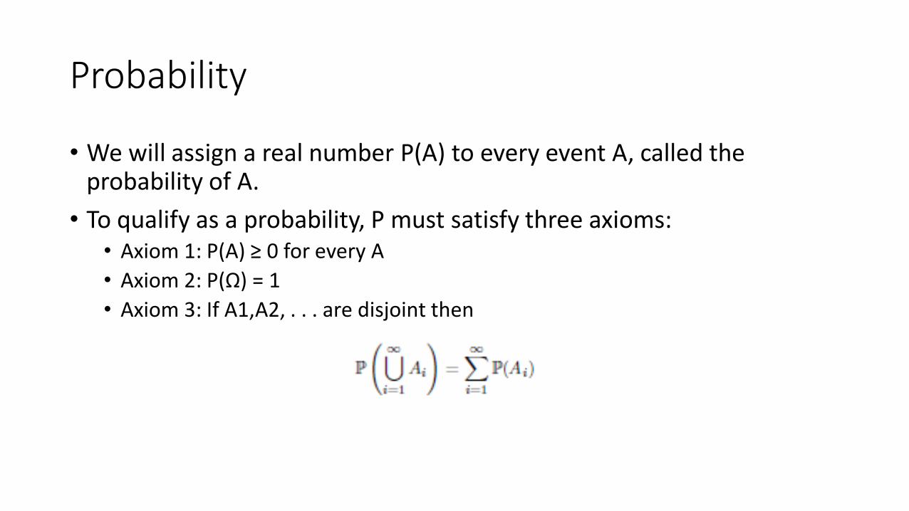
• We will assign a real number P(A) to every event A, called the probability of A.

• To qualify as a probability, P must satisfy three axioms:• Axiom 1: P(A) ≥ 0 for every A

• Axiom 2: P(Ω) = 1

• Axiom 3: If A1,A2, . . . are disjoint then

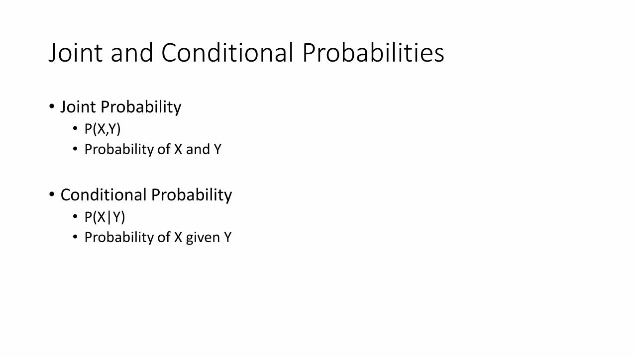
Joint and Conditional Probabilities

• Joint Probability• P(X,Y)

• Probability of X and Y

• Conditional Probability• P(X|Y)

• Probability of X given Y

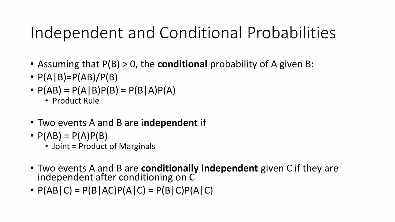
Independent and Conditional Probabilities

• Assuming that P(B) > 0, the conditional probability of A given B:• P(A|B)=P(AB)/P(B)• P(AB) = P(A|B)P(B) = P(B|A)P(A)

• Product Rule

• Two events A and B are independent if• P(AB) = P(A)P(B)

• Joint = Product of Marginals

• Two events A and B are conditionally independent given C if they are independent after conditioning on C

• P(AB|C) = P(B|AC)P(A|C) = P(B|C)P(A|C)

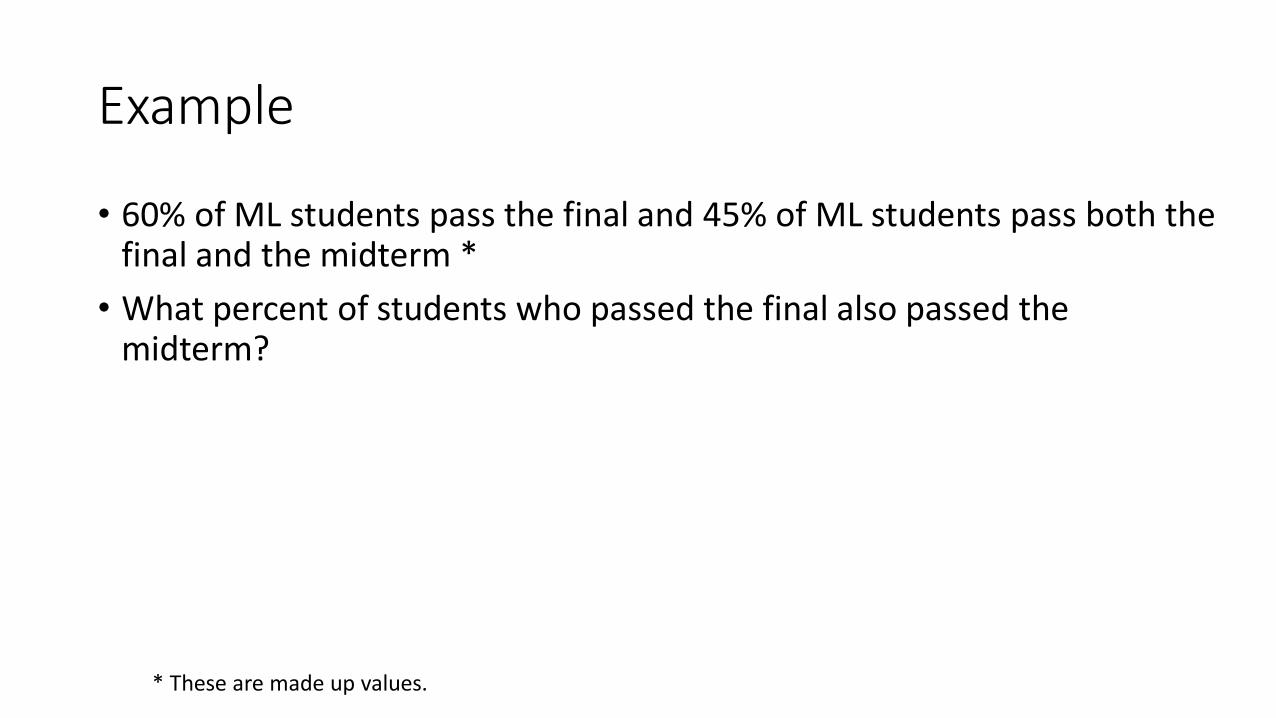
Example

• 60% of ML students pass the final and 45% of ML students pass both the final and the midterm *

• What percent of students who passed the final also passed the midterm?

* These are made up values.

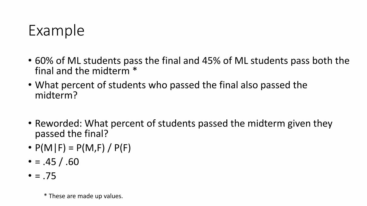
Example

• 60% of ML students pass the final and 45% of ML students pass both the final and the midterm *

• What percent of students who passed the final also passed the midterm?

• Reworded: What percent of students passed the midterm given they passed the final?

• P(M|F) = P(M,F) / P(F)

• = .45 / .60

• = .75

* These are made up values.

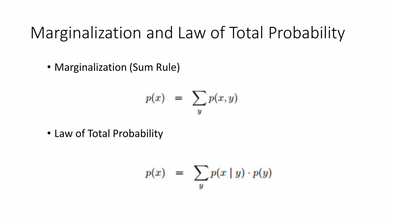
Marginalization and Law of Total Probability

• Marginalization (Sum Rule)

• Law of Total Probability

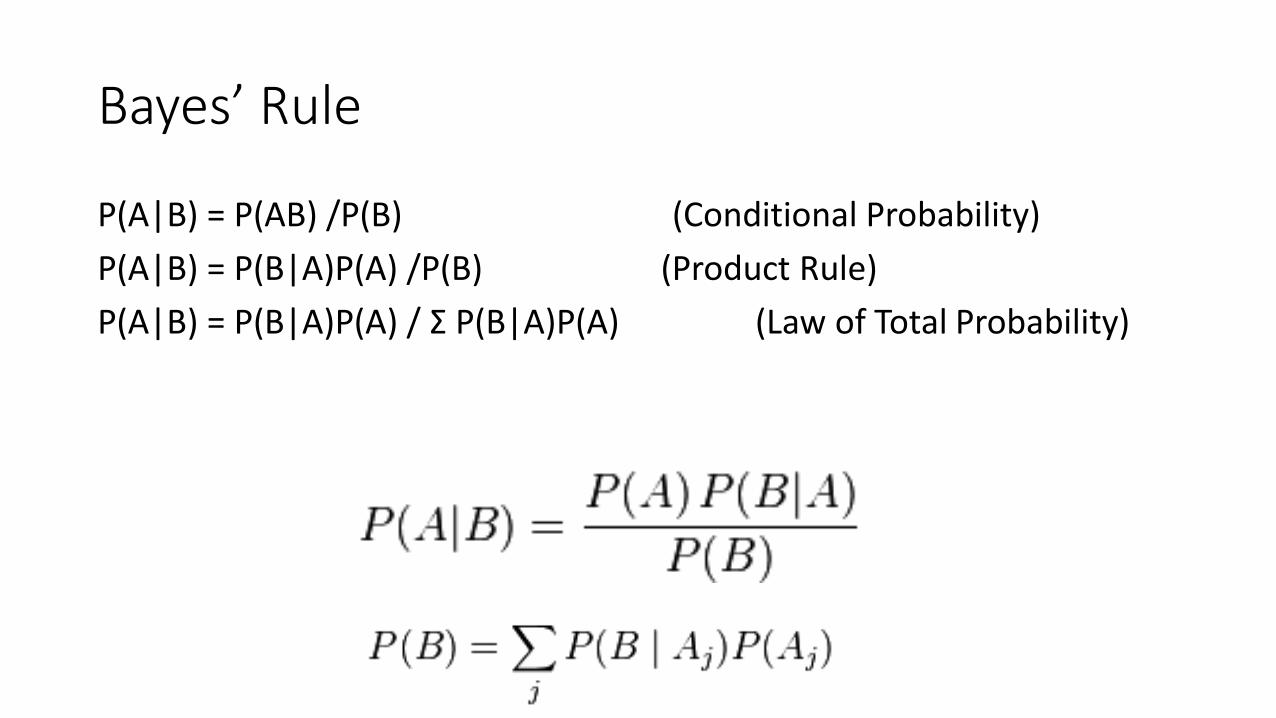
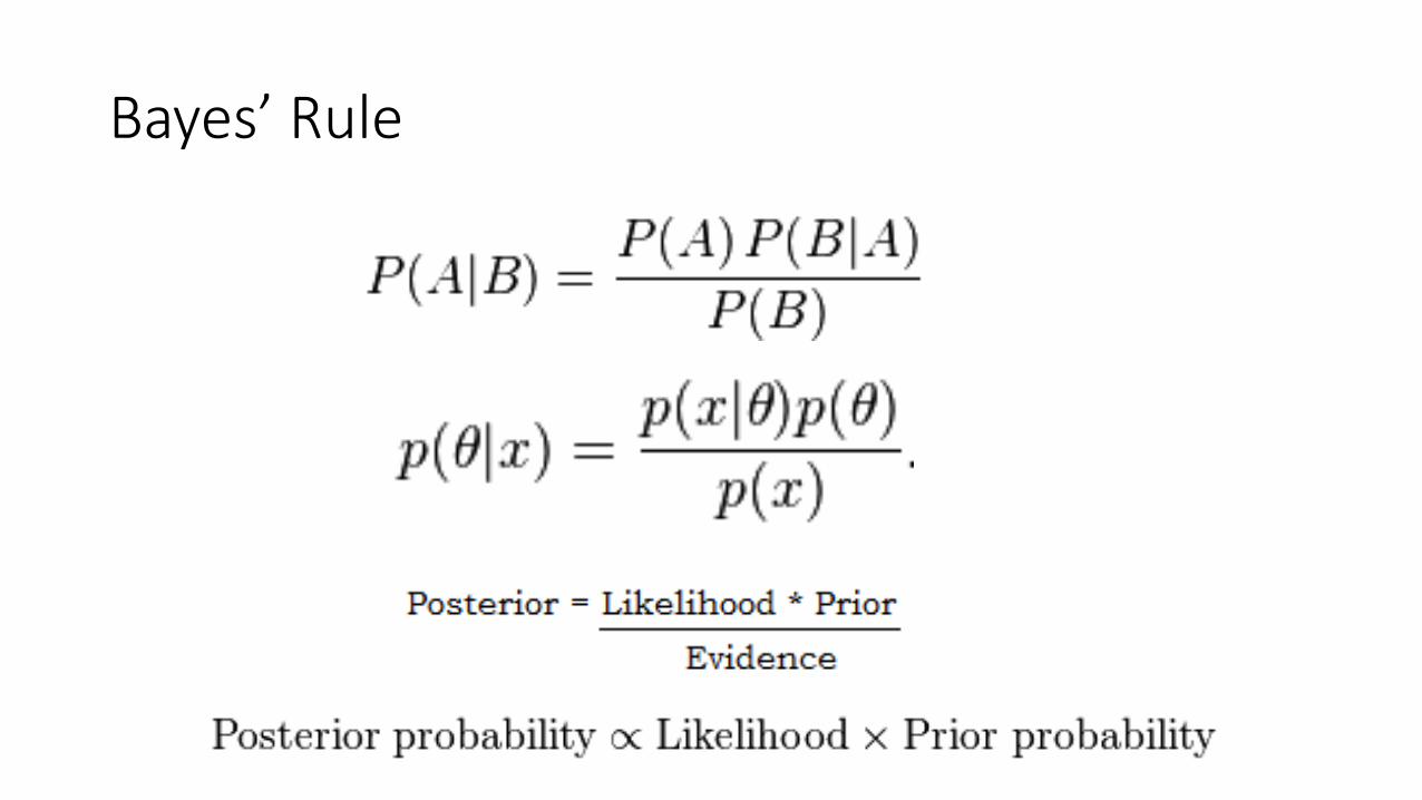
Bayes’ Rule

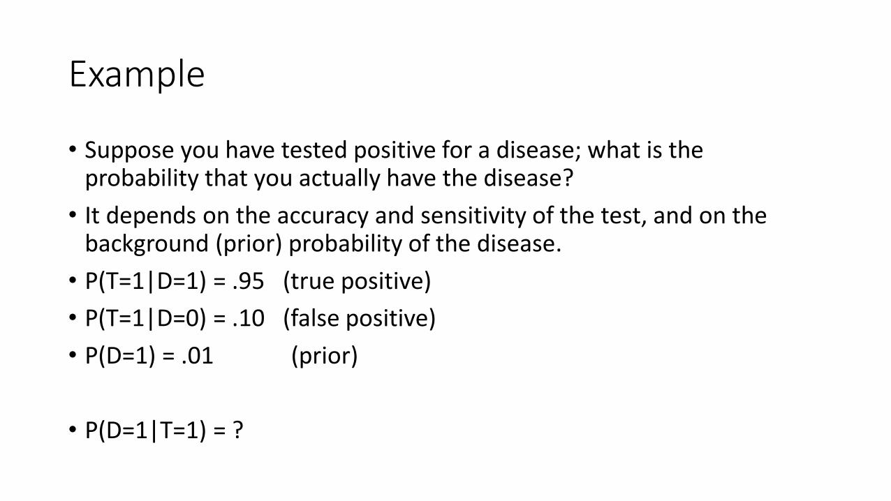
Example

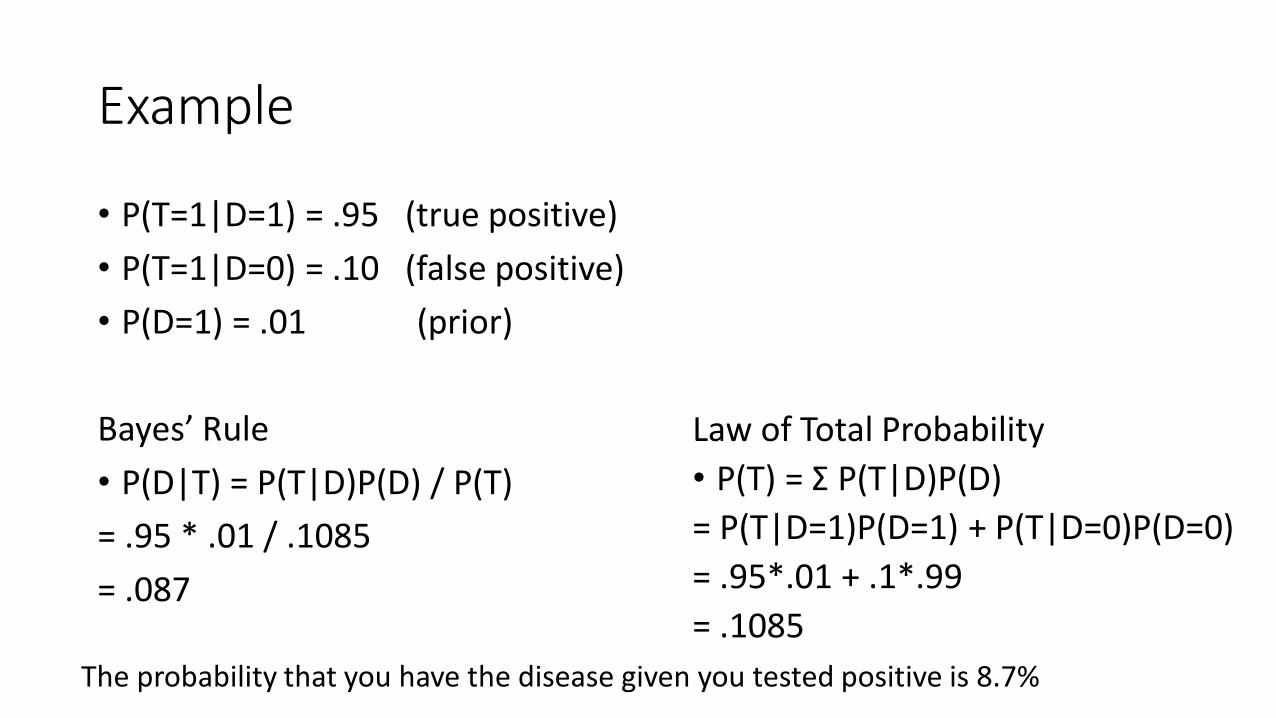
• Suppose you have tested positive for a disease; what is the probability that you actually have the disease?

• It depends on the accuracy and sensitivity of the test, and on the background (prior) probability of the disease.

• P(T=1|D=1) = .95 (true positive)

• P(T=1|D=0) = .10 (false positive)

• P(D=1) = .01 (prior)

• P(D=1|T=1) = ?

Example

• P(T=1|D=1) = .95 (true positive)

• P(T=1|D=0) = .10 (false positive)

• P(D=1) = .01 (prior)

Bayes’ Rule

• P(D|T) = P(T|D)P(D) / P(T)

= .95 * .01 / .1085

= .087

Law of Total Probability

• P(T) = Σ P(T|D)P(D)

= P(T|D=1)P(D=1) + P(T|D=0)P(D=0)

= .95*.01 + .1*.99

= .1085

The probability that you have the disease given you tested positive is 8.7%

Random Variable

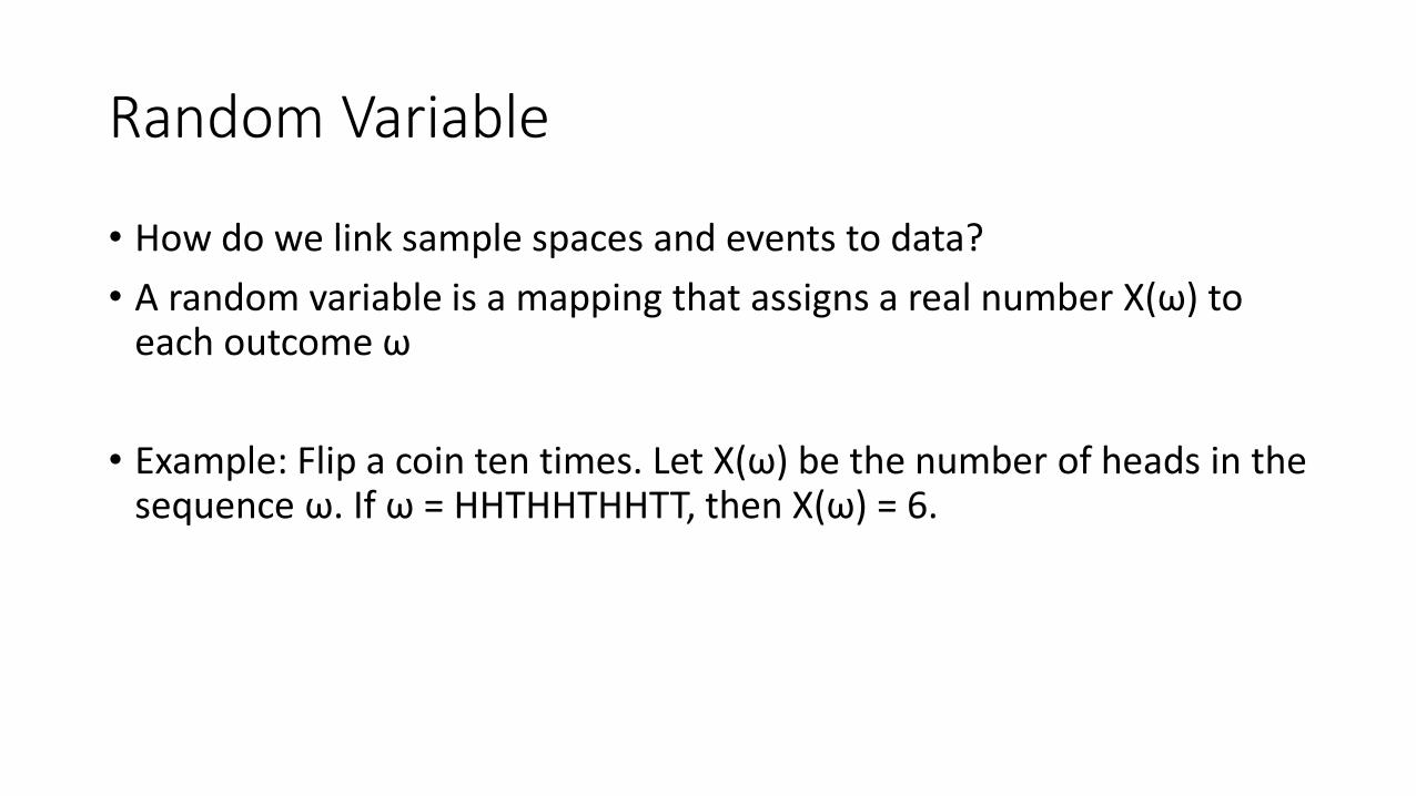
• How do we link sample spaces and events to data?

• A random variable is a mapping that assigns a real number X(ω) to each outcome ω

• Example: Flip a coin ten times. Let X(ω) be the number of heads in the sequence ω. If ω = HHTHHTHHTT, then X(ω) = 6.

Discrete vs Continuous Random Variables

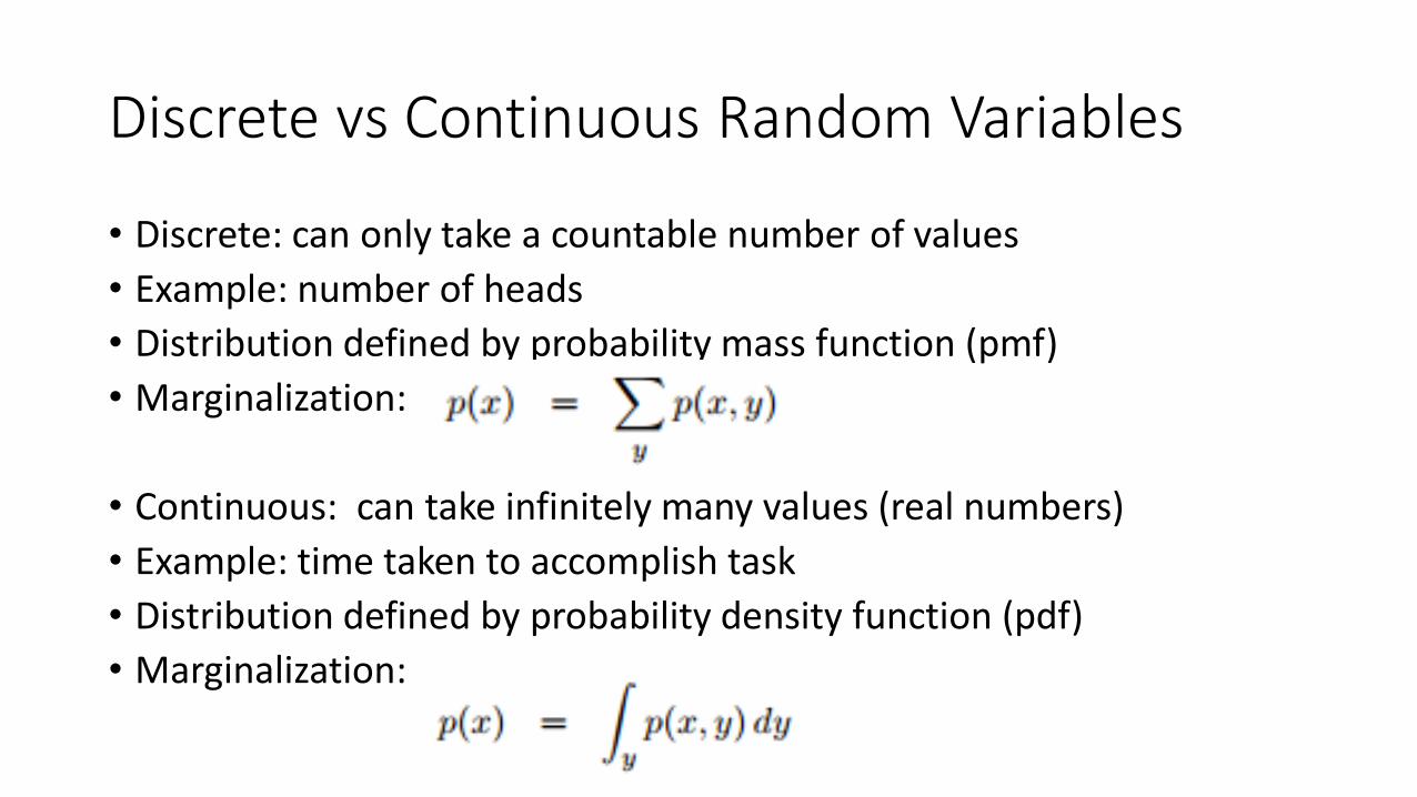
• Discrete: can only take a countable number of values

• Example: number of heads

• Distribution defined by probability mass function (pmf)

• Marginalization:

• Continuous: can take infinitely many values (real numbers)

• Example: time taken to accomplish task

• Distribution defined by probability density function (pdf)

• Marginalization:

Probability Distribution Statistics

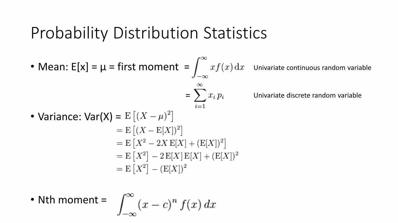
• Mean: E[x] = μ = first moment =

• Variance: Var(X) =

• Nth moment =

Univariate continuous random variable

Univariate discrete random variable=

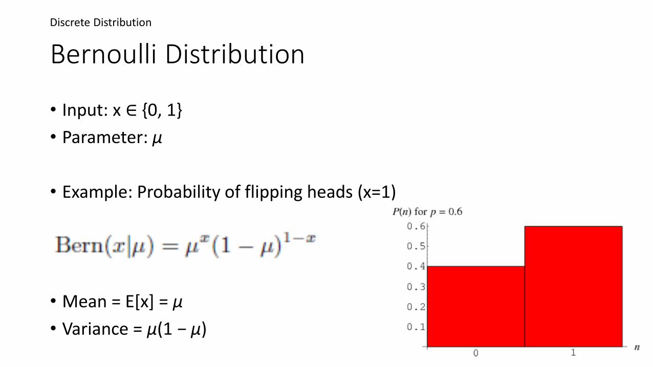
Bernoulli Distribution

• Input: x ∈ {0, 1}

• Parameter: μ

• Example: Probability of flipping heads (x=1)

• Mean = E[x] = μ

• Variance = μ(1 − μ)

Discrete Distribution

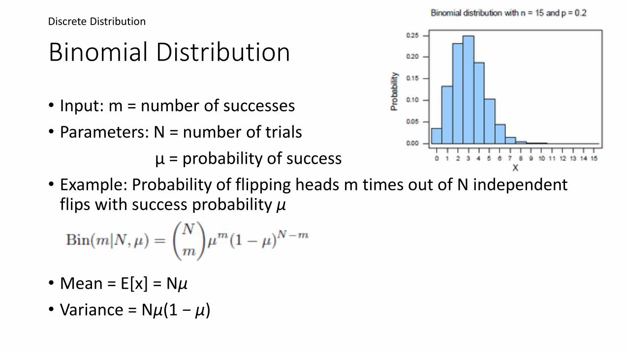
Binomial Distribution

• Input: m = number of successes

• Parameters: N = number of trials

μ = probability of success

• Example: Probability of flipping heads m times out of N independent flips with success probability μ

• Mean = E[x] = Nμ

• Variance = Nμ(1 − μ)


Multinomial Distribution

• The multinomial distribution is a generalization of the binomial distribution to k categories instead of just binary (success/fail)

• For n independent trials each of which leads to a success for exactly one of k categories, the multinomial distribution gives the probability of any particular combination of numbers of successes for the various categories

• Example: Rolling a die N times


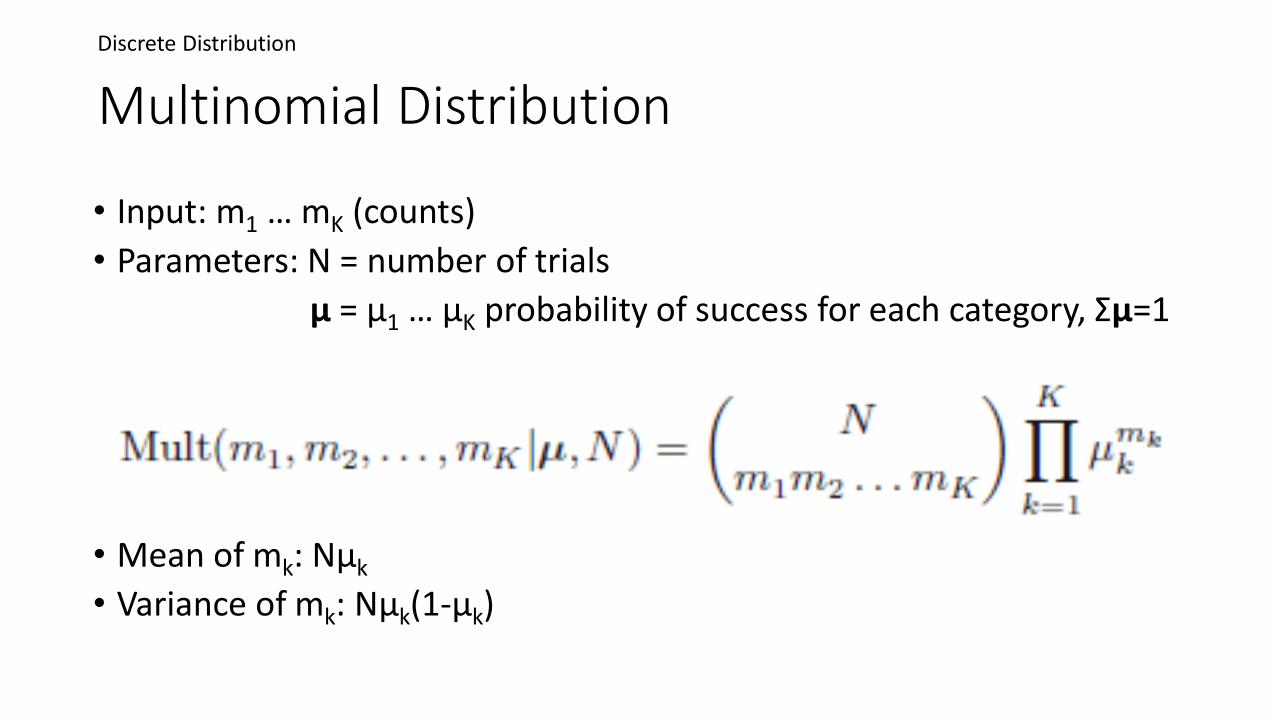
Multinomial Distribution

• Input: m1 … mK (counts)

• Parameters: N = number of trials

μ = μ1 … μK probability of success for each category, Σμ=1

• Mean of mk: Nµk

• Variance of mk: Nµk(1-µk)


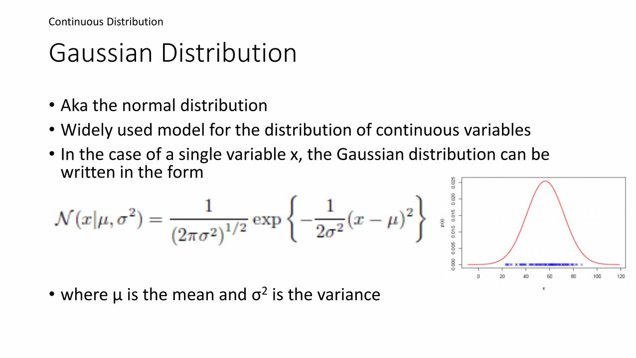
Gaussian Distribution

• Aka the normal distribution

• Widely used model for the distribution of continuous variables

• In the case of a single variable x, the Gaussian distribution can be written in the form

• where μ is the mean and σ2 is the variance

Continuous Distribution

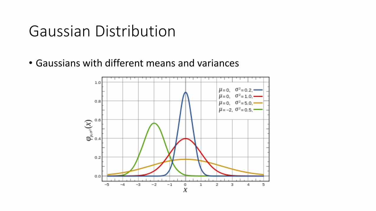
Gaussian Distribution

• Gaussians with different means and variances

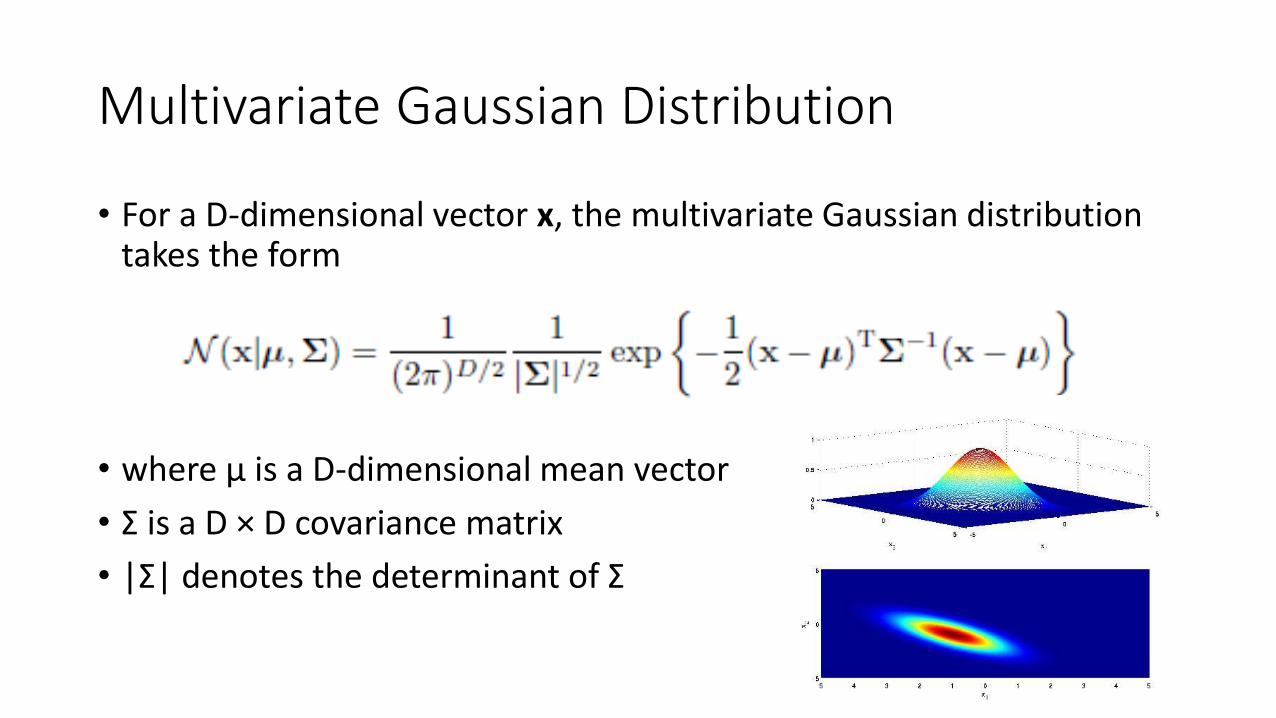
Multivariate Gaussian Distribution

• For a D-dimensional vector x, the multivariate Gaussian distribution takes the form

• where μ is a D-dimensional mean vector

• Σ is a D × D covariance matrix

• |Σ| denotes the determinant of Σ

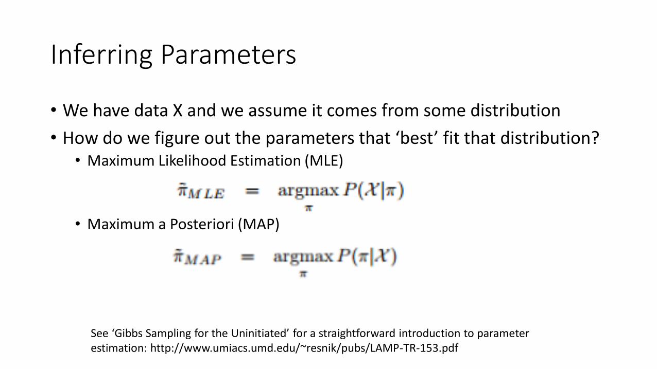
Inferring Parameters

• We have data X and we assume it comes from some distribution

• How do we figure out the parameters that ‘best’ fit that distribution?• Maximum Likelihood Estimation (MLE)

• Maximum a Posteriori (MAP)

See ‘Gibbs Sampling for the Uninitiated’ for a straightforward introduction to parameter estimation: http://www.umiacs.umd.edu/~resnik/pubs/LAMP-TR-153.pdf

I.I.D.

• Random variables are independent and identically distributed (i.i.d.) if they have the same probability distribution as the others and are all mutually independent.

• Example: Coin flips are assumed to be IID

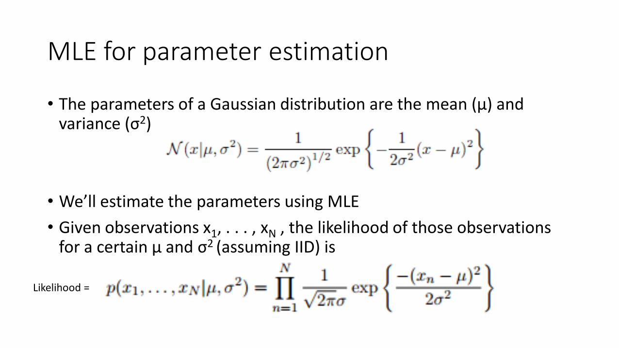
MLE for parameter estimation

• The parameters of a Gaussian distribution are the mean (µ) and variance (σ2)

• We’ll estimate the parameters using MLE

• Given observations x1, . . . , xN , the likelihood of those observations for a certain µ and σ2 (assuming IID) is

Likelihood =

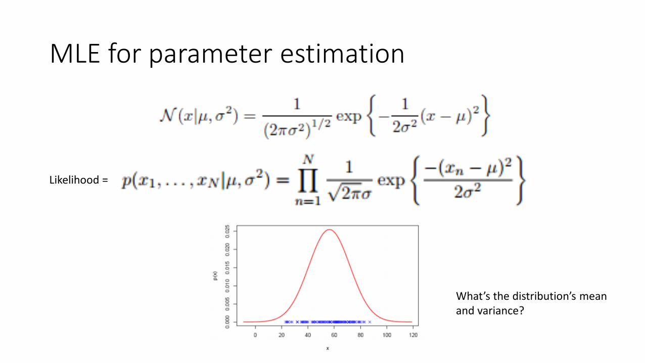
MLE for parameter estimation

What’s the distribution’s mean and variance?

Likelihood =

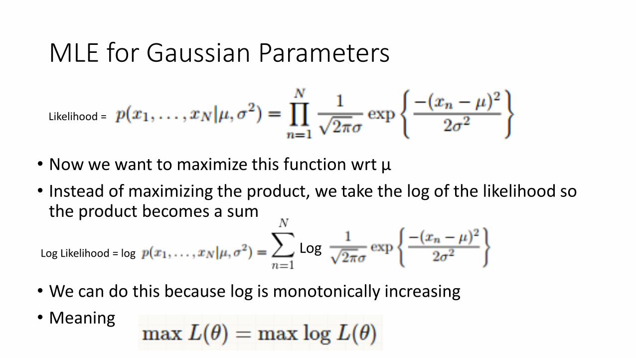
MLE for Gaussian Parameters

• Now we want to maximize this function wrt µ

• Instead of maximizing the product, we take the log of the likelihood so the product becomes a sum

• We can do this because log is monotonically increasing

• Meaning

Likelihood =

Log Likelihood = log Log


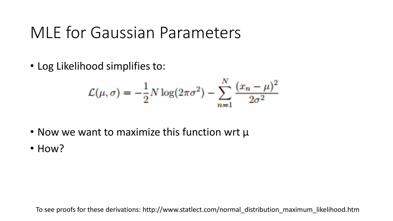
• Log Likelihood simplifies to:

• Now we want to maximize this function wrt μ

• How?

To see proofs for these derivations: http://www.statlect.com/normal_distribution_maximum_likelihood.htm


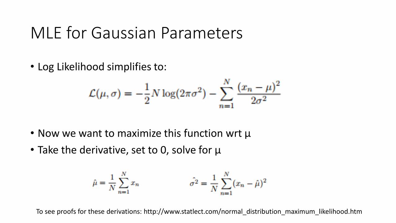
• Log Likelihood simplifies to:

• Now we want to maximize this function wrt μ

• Take the derivative, set to 0, solve for μ

To see proofs for these derivations: http://www.statlect.com/normal_distribution_maximum_likelihood.htm

Maximum Likelihood and Least Squares

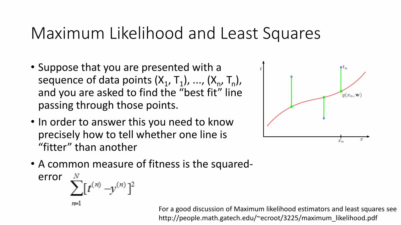
• Suppose that you are presented with a sequence of data points (X1, T1), ..., (Xn, Tn), and you are asked to find the “best fit” line passing through those points.

• In order to answer this you need to know precisely how to tell whether one line is “fitter” than another

• A common measure of fitness is the squared-error

For a good discussion of Maximum likelihood estimators and least squares seehttp://people.math.gatech.edu/~ecroot/3225/maximum_likelihood.pdf


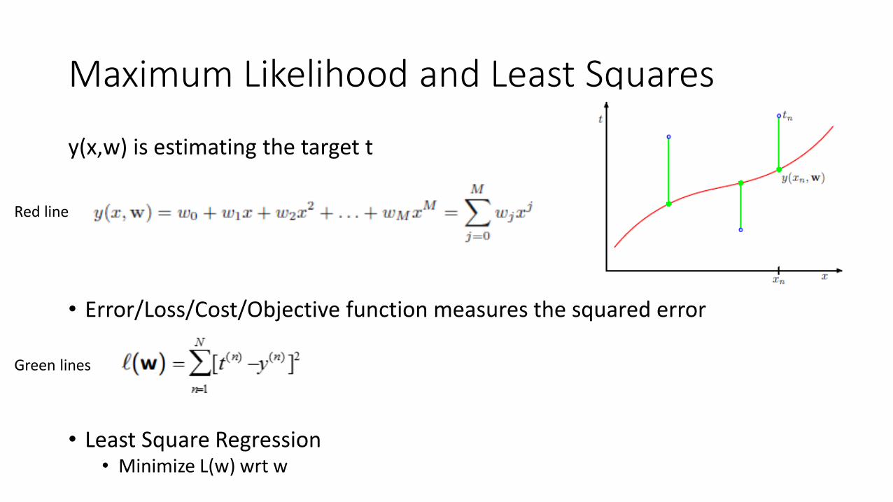
y(x,w) is estimating the target t

• Error/Loss/Cost/Objective function measures the squared error

• Least Square Regression• Minimize L(w) wrt w

Green lines

Red line


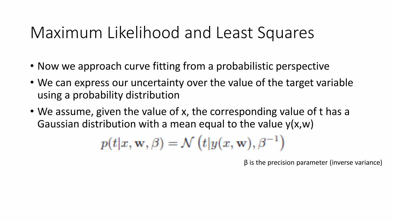
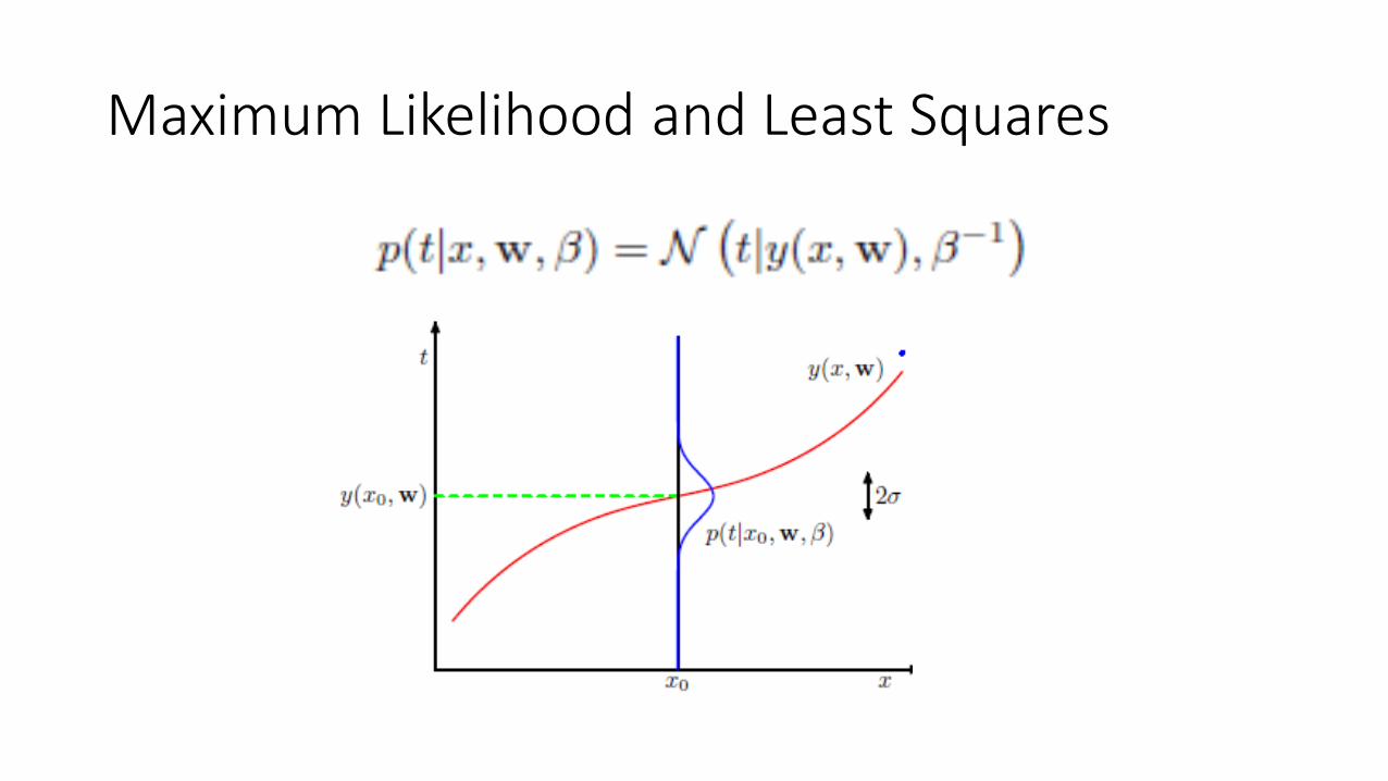
• Now we approach curve fitting from a probabilistic perspective

• We can express our uncertainty over the value of the target variable using a probability distribution

• We assume, given the value of x, the corresponding value of t has a Gaussian distribution with a mean equal to the value y(x,w)

β is the precision parameter (inverse variance)


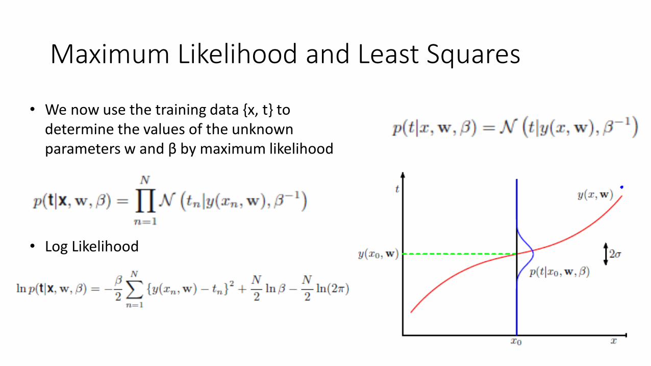
• We now use the training data {x, t} to determine the values of the unknown parameters w and β by maximum likelihood

• Log Likelihood


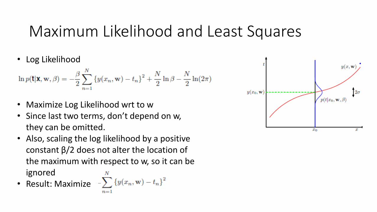
• Log Likelihood

• Maximize Log Likelihood wrt to w• Since last two terms, don’t depend on w,

they can be omitted. • Also, scaling the log likelihood by a positive

constant β/2 does not alter the location of the maximum with respect to w, so it can be ignored

• Result: Maximize


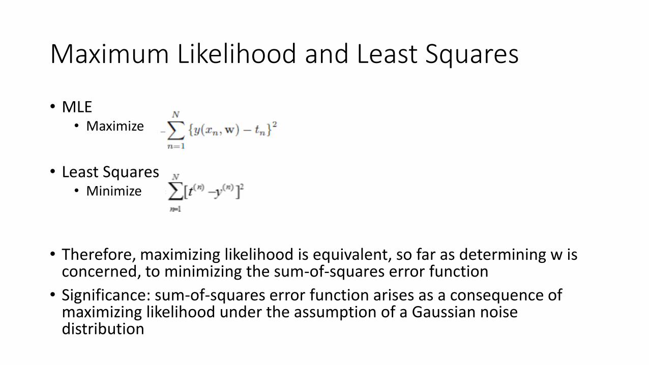
• MLE• Maximize

• Least Squares• Minimize

• Therefore, maximizing likelihood is equivalent, so far as determining w is concerned, to minimizing the sum-of-squares error function

• Significance: sum-of-squares error function arises as a consequence of maximizing likelihood under the assumption of a Gaussian noise distribution

Questions?

Probability Basics for Machine Learningurtasun/courses/CSC411/tutorial1.pdf · Joint and...

Documents

Transcript of Probability Basics for Machine Learningurtasun/courses/CSC411/tutorial1.pdf · Joint and...